bcilab and applications to eeg cognitive interfaces
TRANSCRIPT

BCILAB and Applications to EEG Cognitive Interfaces
Christian A. Kothe
SCCN, INC, UCSD

Outline
1. High-level View
2. Application Areas and Examples
3. Basic Underlying Theory
4. The BCILAB Toolbox
5. GUI and Scripting Tour
6. Methods Tour
7. Current and Future Directions
A. Further Reading

1 High-Level Overview

BCI: Our Working Definition
• “A system which takes a biosignal measured from a
person and predicts (in real time / on a single-trial
basis) some abstract aspect of the person's cognitive state.”
BCI
(inference/
estimation)
Biosignal State Predictions

Biosignals and other Inputs
• Brain Signals: EEG, fNIRS, MEG, fMRI, ECoG, …
• Peripheral Measures: ECG, EMG, EOG, GSR, Respiration, Gaze/Pupillometry, Motion Capture
• Context Information: Program/System State, Vehicle Speed, ...
Biosignal BCI
(inference/
estimation)

BCI Estimates/Predictions
• Any aspect of the physical brain state that can be recovered from observable signals (discrete, continuous, multivariate, …)
• Tonic state: degree of “relaxation”, cognitive load,…
• Phasic state: attention deployment, imagined vowel
• Event-related state: surprised/not surprised, committed error, event noticed/not noticed, …
State Predictions
BCI
(inference/
estimation)

SCCN Software Tools for BCI
BCI
(inference/
estimation)
Lab Streaming Layer (LSL) code.google.com/p/labstreaminglayer
BCILAB ftp://sccn.ucsd.edu/pub/bcilab
sccn.ucsd.edu/wiki/BCILAB
Simulation and Neuroscience Application
Platform (SNAP) ftp://sccn.ucsd.edu/pub/SNAP
EEGLAB, MoBILAB, SIFT, … (not discussed here today)

2 Application Areas and Examples

Communication and Control for the Severely Disabled
• Severe Disabilities: Tetraplegia, Locked-in syndrome
• Speller Programs, Wheelchairs, Robots, …
P300 Speller KU Leuven Brain2Robot (Fraunhofer FIRST)

Other Health Uses
• Sleep Stage Recognition, Neurorehabilitation
iBrain Takata et al., 2011

Operator Monitoring
• Braking Intent, Lane-Change Intent, Workload, Fatigue, Alertness, Attention, …
Haufe et al., 2011 The MITRE Corp., 2011

Entertainment, Social, etc.
• Control by Thought, Mood Assessment/Display
Jedi Game Prototype necomimi “neurowear”

Neuroscience
• Multivariate Pattern Analysis / Brain Imaging
Kothe et al., 2011

4 The BCILAB Toolbox

Software Environment For:
• Brain-Computer Interface Design (Cognitive Monitoring)
• Methods Research: – Design & rapid prototyping of new methods &
methods from literature
– Offline testing, performance evaluation & batch comparison, visualizations
– Simulated online testing
• Rapid Prototyping: – Real-time use and testing of BCIs
– Prototype deployment

Basic Goals
• Usable by beginners and experts to serve both the EEGLAB community and advanced needs
• Include a large array of methods, both conventional and state-of-the art, to rapidly set up well-performing BCIs and conduct broad comparison studies
• Provide convenient plugin frameworks and reusable backend tools to allow for rapidly prototyping of methods

Facts & Figures
• Developed since 2010 at SCCN, UCSD (primarily by me)
• Precursor was the PhyPA toolbox (Kothe & Zander, 2006-’09)
• Built on top of EEGLAB (Delorme & Makeig, 2004)
• The largest open-source BCI toolbox by methods and algorithms (100+) as of 2011
• Offline and online processing both in MATLAB, same code base, Win/Linux/MacOS, 32/64bit
• Extensive documentation (hundreds of pages of help text, manual, wiki, 400+ lecture slides online)

BCILAB Sample GUI
http://sccn.ucsd.edu/wiki/BCILAB ftp://sccn.ucsd.edu/pub/bcilab

BCILAB Sample Script
• Benchmarking 5 state-of-the-art methods on a 136-subject data set (on a cluster):

Toolbox Organization
Dependencies CVX BNT GUI utils
Driver I/O
EEGLAB LIBSVM GLMNET …
Infrastructure GUI
generation cluster
computing disk
caching helper
functions environment
services
Signal Processing Machine Learning BCI Paradigms Devices
Plugins
ICA SSA FIR
IIR FFT …
LDA QDA
GMM SVM …
DAL CSP Spec-CSP
ERP RSSD …
TCP
BCI2000 …
OSC
Framework
Approach Definition
Offline Evaluation
Visualization Online
Execution
GUI / Scripting Interfaces
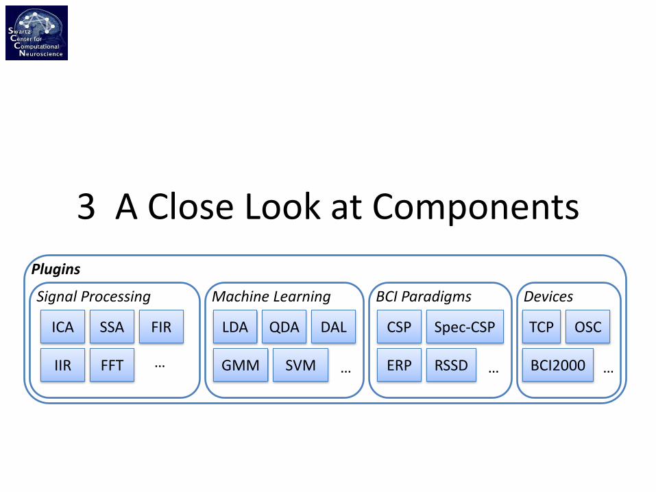
3 A Close Look at Components
Signal Processing Machine Learning BCI Paradigms Devices
Plugins
ICA SSA FIR
IIR FFT …
LDA QDA
GMM SVM …
DAL CSP Spec-CSP
ERP RSSD …
TCP
BCI2000 …
OSC

Component 1: Predictive Mapping

Central Predictive Mapping
• A BCI (with limited memory of the past) can be viewed as a mathematical function f:
• The functional form is arbitrary, for example
𝑦 = sign(var(𝑾𝑿) + 𝑏)
• The mapping involves free parameters, here W and b, and data from a sliding window X
y = f(X); X= y= “subj. excited” (+1) “subj. not excited” (-1)
Choice of a Functional Form
• Reflects the relationship between observation (data segment X) and desired output (cognitive state parameter y)
• Based on some assumed generative mechanism (forward model) – or ad hoc
• Note: Functional form is the inverse mapping!

Choice of a Functional Form
• Reflects the relationship between observation (data segment X) and desired output (cognitive state parameter y)
• Based on some assumed generative mechanism (forward model) – or ad hoc
• Remember: Functional form is the inverse mapping!

Key Ingredient: Spatial Filter
• Linear inverse of volume conduction effect between sources S and channels X 𝑿 = 𝑨𝑺 (forward) 𝑺 = 𝑾𝑿 (inverse)
W A=W-1

Component 2: Signal Processing

Role of Signal Processing
• BCILAB allows to implemented BCIs using a network of digital signal processing blocks (“filters”)
• Relevant filter classes: Spatial Filters, Temporal Filters, Spectral Filters, Spatio-Temporal Filters, Domain Transforms (e.g. DFT)
Filter Filter
Filter
Filter
Filter Graph EEG
EMG
Control Signal

Role of Signal Processing
• Concrete Toy Example: Feed the amplitude of a brain idle oscillation (e.g. 10 Hz alpha associated with relaxation) from one EEG channel back to the user/subject
• This produces the same output as the following functional-style description (T is a temporal filter matrix), but is computationally less costly:
FIR Band-pass (8-13 Hz) Squaring
Moving Average
Square Root or
Logarithm
Running Variance
𝑦𝑖(𝑛) = 𝑏𝑘𝑥𝑖 (𝑛 − 𝑡)
𝑚
𝑘=0
𝑦𝑖(𝑛) = 1
𝑚 − 1 𝑥𝑖 (𝑛 − 𝑘)
𝑚
𝑘=0
𝑦𝑖(𝑛) = 𝑥𝑖 (𝑛)2 𝑦𝑖(𝑛) = log 𝑥𝑖 (𝑛)

Filter Components In Practice
• Filters can operate on continuous signals…
• … or on segmented (“epoched”) signals:
Continuous-Data Filters
Epoched-Data Filters
EEG = flt_selchans(EEG,{‘C3’,’C4’,’Cz’})
[EEG,State] = flt_resample(EEG,200,State)

Combined Online Processing
• Both frameworks are complementary, rather than contradictory, and are in practice often used in combination, e.g. to minimize computational costs
Filter Filter
Filter
Filter
Filter Graph
Prediction Function
EEG
EMG
tPred
y = f(X)
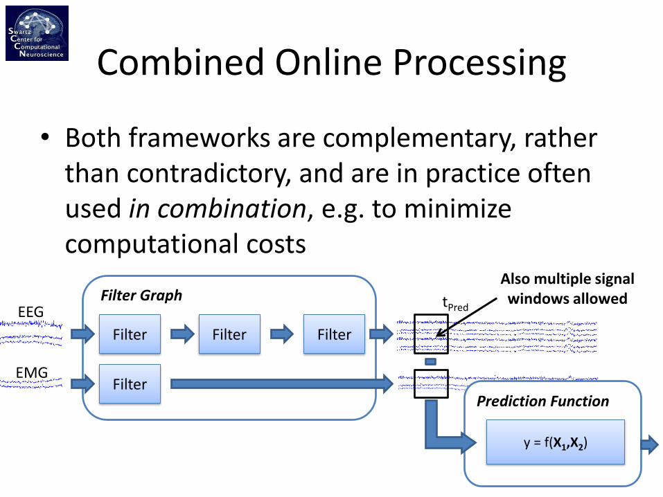
Combined Online Processing
• Both frameworks are complementary, rather than contradictory, and are in practice often used in combination, e.g. to minimize computational costs
Filter Filter
Filter
Filter
Filter Graph
Prediction Function
EEG
EMG
tPred
y = f(X1,X2)
Also multiple signal windows allowed

Component 3: Machine Learning

The Problem of Unknown Parameters
• Processing depends on unknown parameters (person-specific, task-specific, otherwise variable) – e.g., per-sensor weights as below:
Blankertz et al. 2007

Reasons for Parameter Uncertainty
• Folding of cortex differs between any two persons
• Relevant functional map differs across individuals
• Sensor locations differ across recording sessions
• Brain dynamics are non- stationary at all time scales

Solution: Calibration
• Calibration / training data can be used to estimate parameters, during a separate calibration step
Calibration data
BCI Model
Calibration step
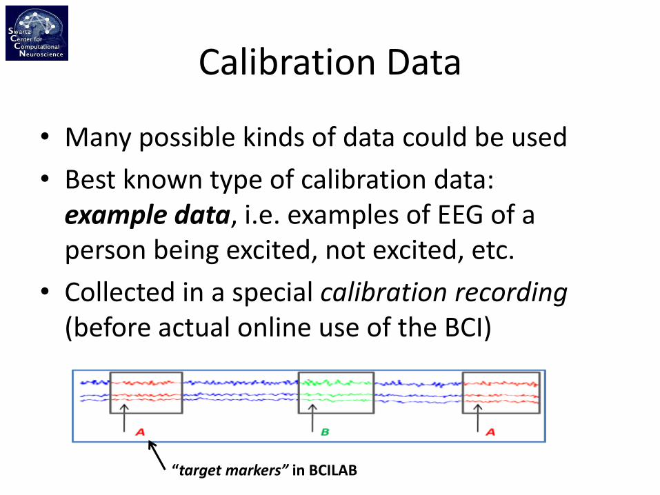
Calibration Data
• Many possible kinds of data could be used
• Best known type of calibration data: example data, i.e. examples of EEG of a person being excited, not excited, etc.
• Collected in a special calibration recording (before actual online use of the BCI)
“target markers” in BCILAB

Big-Picture Information Flow
Filter Filter
Filter
Filter
Filter Graph
Prediction Function
EEG
EMG
y = f(X)
tPred
Learning Function …

Machine Learning Framework
• Large field with 100s of algorithms (LDA, SVM, GMM, ANNs, logistic regression, …)
• Most methods conform to a common framework of a training function and a prediction function
Machine Learning Method (Supervised)
Training function
Prediction function
Data
Labels Model
Pre- dicted Labels
New Data
Model
M = ml_trainsvm(X,y, <extra parameters>)
y_pred = ml_predictsvm(X_new,M)

Machine Learning In Practice
• Often, one trial segment (sample) is extracted for every target marker in the calibration recording and is used as training exemplar Xk
• Its associated label yk can be deduced from the target marker
S2 S1 R1 S1
2 1 1
, , …

Machine Learning In Practice
• Often, one trial segment (sample) is extracted for every target marker in the calibration recording and is used as training exemplar Xk
• Its associated label yk can be deduced from the target marker
S2 S1 R1 S1
2 1 1
, , … Training
function Model
X,y 𝜽

Component 4: Feature Extraction

Feature Extraction
• Caveat: Off-the-shelf machine learning methods often do not work very well when applied to raw signal segments of the calibration recording
– too high-dimensional (too many parameters to fit)
– too complex structure to be captured (too much modeling freedom, requires domain-specific assumptions)
1000s of degrees of freedom!
Feature Extraction
• Typical Solution: Introduce additional mapping (called “feature extraction”) from raw signal segments onto feature vectors which extracts the key features of a raw observation
– output is usually of lower dimensionality
– hopefully statistically “better” distributed (easier to handle for machine learning)

Concrete Example Task
• Flanker Task: The experiment consists of a sequence of ca. 330 trials with inter-trial interval of 2s +/- 1.5s
• At the beginning of each trial, an arrow is presented centrally (pointing either left or right)
• The arrow is flanked by congruent or incongruent “flanker” arrows (preceding the center by a few ms):
• The subject is asked to press the left or right button, according to the central arrow direction, and makes frequent errors (ca. 25%)

Approach
• Calibration recording is band-pass filtered between 0.5Hz and 15Hz
– 0.5Hz lower edge removes drifts
– 15Hz upper edge leaves enough room for sharp ERP features
• Epochs are extracted for each trial and label is set to A for incorrect trials and B for corrects

Actual Data
• Time courses for all trials super-imposed (color-coded by class) – but here different task

Extracted Epochs Channel time courses under Condition B
Channel time courses under Condition A
Three sample trials (out of 100) shown: mean, -1 std. dev, +1 std. dev
Response (A or B)

Extracting Linear Features
For each trial segment, calculate signal mean in 3 time sub-windows ( 3-dim feature vector)
f1 f2 f3
f1
f2 f3

Resulting Feature Space
• Plotting the 3-element feature vectors for all error trials in red, and non-error trials in green, we obtain two distributions in a 3d space:
Note that across all channels this space has in fact 3 x #channels dimensions!

• Including the feature extraction, the analysis process is as follows:
ML with Feature Extraction
S2 S1 R1 S1
2 1 1
, , …
Training function Model
X,y
Extract Features
𝑓1𝑓2⋮
𝑓1𝑓2⋮
𝑓1𝑓2⋮
, ,
2 1 1
…
𝜽

Machine Learning Continued
• The feature vectors are passed on to a machine learning function (e.g., Linear Discriminant Analysis)
f1
f2 f3
e.g., LDA

Machine Learning Continued
• The feature vectors are passed on to a machine learning function (e.g., Linear Discriminant Analysis)
• … which determines a parametric predictive mapping
f1
f2 f3
e.g., LDA
𝜽

Simple 2-class LDA In a Nutshell
• Given feature vectors 𝒙𝑘 (in vector form) in 𝒞1 and 𝒞2,
𝝁𝑖 = 1
𝒞𝑖 𝒙𝑘
𝑘∈𝒞𝑖
, 𝜮𝑖 = 𝒙𝑘 − 𝝁𝑖 𝒙𝑘 − 𝝁𝑖⊺
𝑘∈𝒞𝑖
𝜽 = 𝜮1 + 𝜮2
−1 𝝁2 − 𝝁1 , b = 𝜽⊺ 𝝁1 + 𝝁2 /2
• Caveat: θ often high-dimensional but only few trials available
• Can use a regularized estimator instead, here using shrinkage; instead of Σ𝑖, we use Σ 𝑖 above:
Σ 𝑖 = 1 − 𝜆 Σ𝑖 + 𝜆𝑰
𝜽
b

Resulting Predictive Mapping and Model
• LDA produces parameters of a linear mapping
y = 𝜽𝒙 − 𝑏
• For classification, the mapping is actually non-linear:
y = sign(𝜽𝒙 − 𝑏)
• The learned model with its person-specific parameters here consists of (𝜽, 𝑏); generally it could include adapted signal-processing parameters, feature-extraction parameters, etc.

Spatial Filters Visualized
• Topographically mapped, the following filters emerge:
Note: This method (and its close relative using “shrinkage LDA” in particular) yield state-of-the-art Performance on ERPs.

Overall BCI Structure
• BCI paradigms are BCILAB’s way to encapsulate all parts of a BCI approach into one unit (e.g., signal processing, feature extraction, machine learning, …)
Calibration recording(s)
Calibrate
Filter Graph Pre-
dict
BCI Model

Component 5: BCI Performance Evaluation

Overall Evaluation Strategies
• When given calibration data and test data…
• Estimate model parameters (spatial filters, statistics)
Model
Calibration data

Overall Evaluation Strategies
• When given calibration data and test data…
• Estimate model parameters (spatial filters, statistics)
• Apply the model to new data (online / single-trial)
• Measure prediction performance or loss (e.g., mis-classification rate or mean-square error)
Model
Calibration data Future data…
Compute Loss

Overall Evaluation Strategies
• Some implemented loss measures (between known “ground-truth” target labels t and predicted labels p) include mean-square error, mis-classification rate, area under ROC curve, and ca. a dozen others
• Mean-Square Error:
– 𝐿𝑀𝑆𝐸(𝒑, 𝒕) =1
𝑁 (𝒑𝑘 − 𝒕𝑘)
2 𝑘
• Mis-Classification Rate:
– 𝐿𝑀𝐶𝑅(𝒑, 𝒕) = 1
𝑁
1, 𝒑𝑘 ≠ 𝒕𝑘0, 𝒑𝑘 = 𝒕𝑘
𝑘

Overall Evaluation Strategies
• What if there is no second data set?
• split one data set repeatedly into training/test blocks systematically, a.k.a. cross-validation
• Each trial is used for testing once
• Time series data: Prefer block-wise cross-validation over randomized
Training part
Test part
Model

Overall Evaluation Strategies
• Parameter search can be done using cross-validation in a grid search (try all values of free parameters)
• Quite general (e.g. can search for best method)
Best Model
Training Test
For all param. values…

Overall Evaluation Strategies
• Parameter search can be done using cross-validation in a grid search (try all values of free parameters)
• Quite general (e.g. can search for best method)
• However: Cannot directly report “best performance” estimates (=cherry-picked)
Best Model
Training Test
For all param. values…

Overall Evaluation Strategies
• Parameter search can be done using cross-validation in a grid search (try all values of free parameters)
• Quite general (e.g. can search for best method)
• However: Cannot directly report “best performance” estimates (=cherry-picked), except on future data
Best Model
Training Test
For all param. values… Future data…

Overall Evaluation Strategies
• Parameter search can be done using cross-validation in a grid search (try all values of free parameters)
• Alternatively: Parameter search can be nested within an outer cross-validation (“nested cross-validation”)
Test part
Best Model
Training Test
For all param. values…

Overall Evaluation Strategies
• The same strategies can be applied across a collection of data sets (e.g., multiple sessions or multiple subjects), for example “hold-one-subject-out”
• Cross-validation, grid search, nested cross-validation can be farmed out to a cluster in BCILAB, also to compiled workers (= no MATLAB license bottleneck)

Summary

Scope of the Online Framework
Filter Filter
Filter
Filter
Filter Graph
Prediction Function
Extract Features
EEG
EMG
Pre-dict
tPred
Managed by the Online Framework
Managed by the Offline Framework
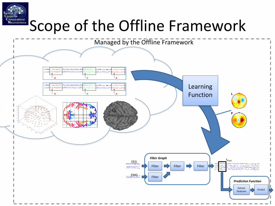
Scope of the Offline Framework
Filter Filter
Filter
Filter
Filter Graph
Prediction Function
EEG
EMG
tPred
Learning Function …
Extract
Features Predict

Offline Framework
Scope of the Offline Framework
• Also Covered: Cross-validation, Grid Search, Nested Cross-Validation
Test part
Best Model
Training Test
For all param. values…

5 GUI and Scripting Tour

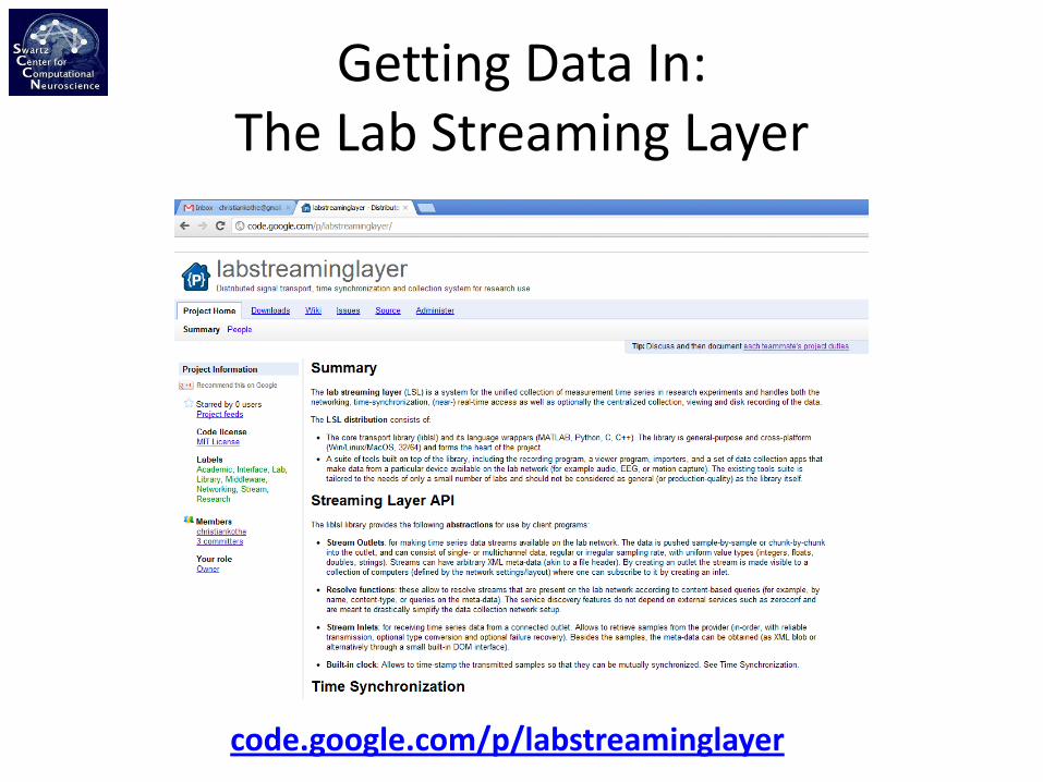
Getting Data In: The Lab Streaming Layer
code.google.com/p/labstreaminglayer

Key Features
• System for the unified access to measurement time series from devices and applications (incl. events)
• Supports centralized collection, viewing and disk recording of the data (unified file format: XDF)
• Handles time-synchronization between multiple streams (to sub-ms precision, up to device uncertainty), networking, fault tolerance
• Library & Examples for C/C++/Python/MATLAB, Win/Linux/MacOS, 32/64bit
• Plugins for EEGLAB, BCILAB, MoBILAB
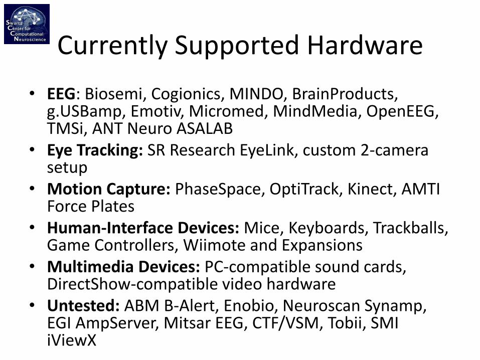
Currently Supported Hardware
• EEG: Biosemi, Cogionics, MINDO, BrainProducts, g.USBamp, Emotiv, Micromed, MindMedia, OpenEEG, TMSi, ANT Neuro ASALAB
• Eye Tracking: SR Research EyeLink, custom 2-camera setup
• Motion Capture: PhaseSpace, OptiTrack, Kinect, AMTI Force Plates
• Human-Interface Devices: Mice, Keyboards, Trackballs, Game Controllers, Wiimote and Expansions
• Multimedia Devices: PC-compatible sound cards, DirectShow-compatible video hardware
• Untested: ABM B-Alert, Enobio, Neuroscan Synamp, EGI AmpServer, Mitsar EEG, CTF/VSM, Tobii, SMI iViewX

Getting Data Out
• BCILAB provides several output protocols (e.g., TCP, OSC, LSL); also allows for custom extensions, e.g., for Presentation or ePrime
• Also supports SNAP natively (our Python-based stimulus-presentation environment)
…
6 Methods Tour

Time-Domain / ERP Baseline
• Traditional linear classifier for event-locked brain responses, usually using LDA
• Time windows manually assigned
• Examples: error recognition, surprise
• State-of-the-art approach, no hand-tuned parameters
• Uses rank-regularized logistic or linear regression
DAL-ERP Windowed Means
(*image: Tomioka et al., 2010)
(*)

Oscillatory Processes Baseline
• State-of-the-art approach, no hand-tuned parameters
• Also uses rank-regularized logistic or linear regression
• Single-step approach, jointly optimal
DAL-OSC Common Spatial Patterns Family
• Filter-Bank CSP (FBCSP): multiple bands/windows
• Diagonal Loading CSP (DLCSP): cov. shrinkage
• Composite CSP (CCSP): covariance prior
• Tikhonov-regularized CSP (TRCSP): filter shrinkage
• Spectrally weighted CSP (Spec-CSP): learning spectral filters from the data
(*image: Tomioka et al., 2010)
(*)
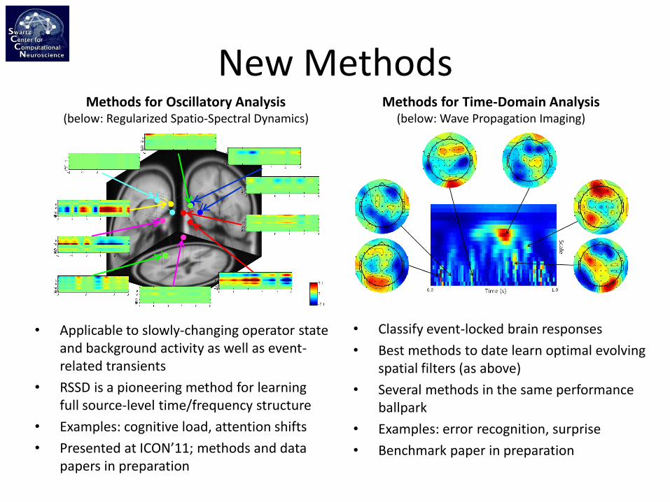
New Methods
• Classify event-locked brain responses
• Best methods to date learn optimal evolving spatial filters (as above)
• Several methods in the same performance ballpark
• Examples: error recognition, surprise
• Benchmark paper in preparation
• Applicable to slowly-changing operator state and background activity as well as event-related transients
• RSSD is a pioneering method for learning full source-level time/frequency structure
• Examples: cognitive load, attention shifts
• Presented at ICON’11; methods and data papers in preparation
Methods for Oscillatory Analysis (below: Regularized Spatio-Spectral Dynamics)
Methods for Time-Domain Analysis (below: Wave Propagation Imaging)

New Methods (Exploratory) Spatio-Spectral Bayes
• A fully Bayesian version of RSSD aimed at neuroscientific modeling
• Allows for extensive statistical analysis of results
• Presented at Sloan-Swartz ‘11
Pattern Alignment Learning
Event
• Finds time-jittered brain processes associated with known events in the work environment
• Radically new approach using joint optimization
• Applications: target event detection and other event-related cognitive responses

7 Future Directions

Current and Future Directions
• Making principled use of anatomical prior knowledge; requires that learned parameters are endowed with anatomically meaningful locations
• First step in this direction: RSSD, using Independent Component Analysis and Dipole Fitting to obtain localized parameters
• Use Beamforming, NFT, …

Current and Future Directions
• Learning models from data spanning multiple persons (using multi-task learning, empirical Bayesian methods, mixed-effects models, etc.)
• Currently only one such implementation in BCILAB (multi-subject-OSR)

Current and Future Directions
• Integrating motion capture information and other peripheral and behavioral measures into BCIs (e.g., eye tracking, facial expression, …)
• Can explain away artifacts and interfering factors, contains rich information about cognitive state by themselves
• Requires deep integration with the MoBILAB toolbox
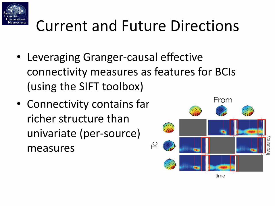
Current and Future Directions
• Leveraging Granger-causal effective connectivity measures as features for BCIs (using the SIFT toolbox)
• Connectivity contains far richer structure than univariate (per-source) measures

A Further Reading

These and Futher Slides:
ftp://sccn.ucsd.edu/pub/bcilab/

BCI Papers Worth Reading
• B. Blankertz, S. Lemm, M. Treder, S. Haufe, and K.-R. Mueller, "Single-trial analysis and classification of ERP components - A tutorial", NeuroImage, vol. 56, no. 2, pp. 814–825, May 2011.
• F. Lotte and C. Guan, “Regularizing common spatial patterns to improve BCI designs: unified theory and new algorithms,” IEEE Transactions on Biomedical Engineering, vol. 58, no. 2, pp. 355-362, Feb. 2011.
• R. Tomioka and K.-R. Mueller, A regularized discriminative framework for EEG analysis with application to brain-computer interface", NeuroImage, vol. 49, no. 1, pp. 415–432, 2010.
• B. Blankertz, G. Dornhege, M. Krauledat, K.-R. Mueller, and G. Curio, "The non-invasive Berlin brain-computer interface: Fast acquisition of effective performance in untrained subjects", NeuroImage, vol. 37, no. 2, pp. 539–550, Aug. 2007.
• M. Grosse-Wentrup, C. Liefhold, K. Gramann, and M. Buss, "Beamforming in noninvasive brain-computer interfaces", IEEE Trans. Biomed. Eng., vol. 56, no. 4, pp. 1209–1219, Apr. 2009.

BCI Surveys
• A. Bashashati, M. Fatourechi, R. K. Ward, and G. E. Birch, "A survey of signal processing algorithms in brain-computer interfaces based on electrical brain signals", J. Neural Eng., vol. 4, no. 2, pp. R32–R57, Jun. 2007.
• F. Lotte, M. Congedo, A. Lecuyer, F. Lamarche, and B. Arnaldi, "A review of classification algorithms for EEG-based brain-computer interfaces", J. Neural Eng., vol. 4, no. 2, pp. R1–R13, Jun. 2007.
• S. Makeig, C. Kothe, T. Mullen, N. Bigdely-Shamlo, Z. Zhang, K. Kreutz-Delgado, "Evolving Signal Processing for Brain–Computer Interfaces", Proc. IEEE, vol. 100, pp. 1567-1584, 2012.

Interesting Technical Papers
• D.P. Wipf and S. Nagarajan, “A Unified Bayesian Framework for MEG/EEG Source Imaging,” NeuroImage, vol. 44, no. 3, February 2009.
• S. Haufe, R. Tomioka, and G. Nolte, “Modeling sparse connectivity between underlying brain sources for EEG/MEG,” Biomedical Engineering, no. c, pp. 1-10, 2010.
• S. Boyd, N. Parikh, E. Chu, and J. Eckstein, “Distributed Optimization and Statistical Learning via the Alternating Direction Method of Multipliers,” Information Systems Journal, vol. 3, no. 1, pp. 1-122, 2010.
• P. Zhao and B. Yu, “On Model Selection Consistency of Lasso,” Journal of Machine Learning Research, vol. 7 pp. 2541-2563, 2006.

Technical Papers, ct’d
• J. Ngiam, A. Khosla, M. Kim, J. Nam, H. Lee, and A. Ng, “Multimodal Deep Learning,” in Proceedings of the 28th International Conference on Machine Learning, 2011.
• K. N. Kay, T. Naselaris, R. J. Prenger, and J. L. Gallant, “Identifying natural images from human brain activity,” Nature, vol. 452, no. 7185, pp. 352-355, Mar. 2008.
• O. Jensen et al., “Using brain-computer interfaces and brain-state dependent stimulation as tools in cognitive neuroscience,” Frontiers in Psychology, vol. 2, p. 100, 2011.
• D.-H. Kim, N. Lu, R. Ma,. Y.-S. Kim, R.-H. Kim, S. Wang, J. Wu, S. M. Won, H. Tao, A. Islam, K. J. Yu, T.-I. Kim, R. Chowdhury, M. Ying, L. Xu, M. Li, H.-J. Cung, H. Keum, M. McCormick, P. Liu, Y.-W. Zhang, F. G. Omenetto, Y Huang, T. Coleman, J. A. Rogers, “Epidermal electronics,” Science vol. 333, no. 6044, 838-843, 2011.

Researchers to Watch
• Klaus-Robert Mueller et al. (TU Berlin) – one of the leading BCI groups http://www.bbci.de/publications.html
• Marcel van Gerven et al. (Donders) – BCI and Neuroscience with a Bayesian approach https://sites.google.com/a/distrep.org/distrep/publications
• Ryota Tomioka (U Tokyo) – known for some technical achievements http://www.ibis.t.u-tokyo.ac.jp/RyotaTomioka
• Karl Friston et al. (UC London) – working on relevant underpinnings for neuroimaging (outside BCI) http://www.fil.ion.ucl.ac.uk/Research/publications.html
• Leading Statisticians and Machine Learners: Michael I. Jordan, Andrew Ng, Lawrence Carin, Zoubin Ghahramani, Francis Bach, Geoffrey Hinton, Ruslan Salakhutdinov, Yeh Whye Teh, David Blei, …

Thanks!
Questions?