BCS in Russia: the end of 50’s –early 60’s

Lev P. Gor’kov

(National High Magnetic Field Laboratory, FSU, Tallahassee)

UIUC, October 10, 2007

( Developing Quantum Field theory approach to superconductivity)

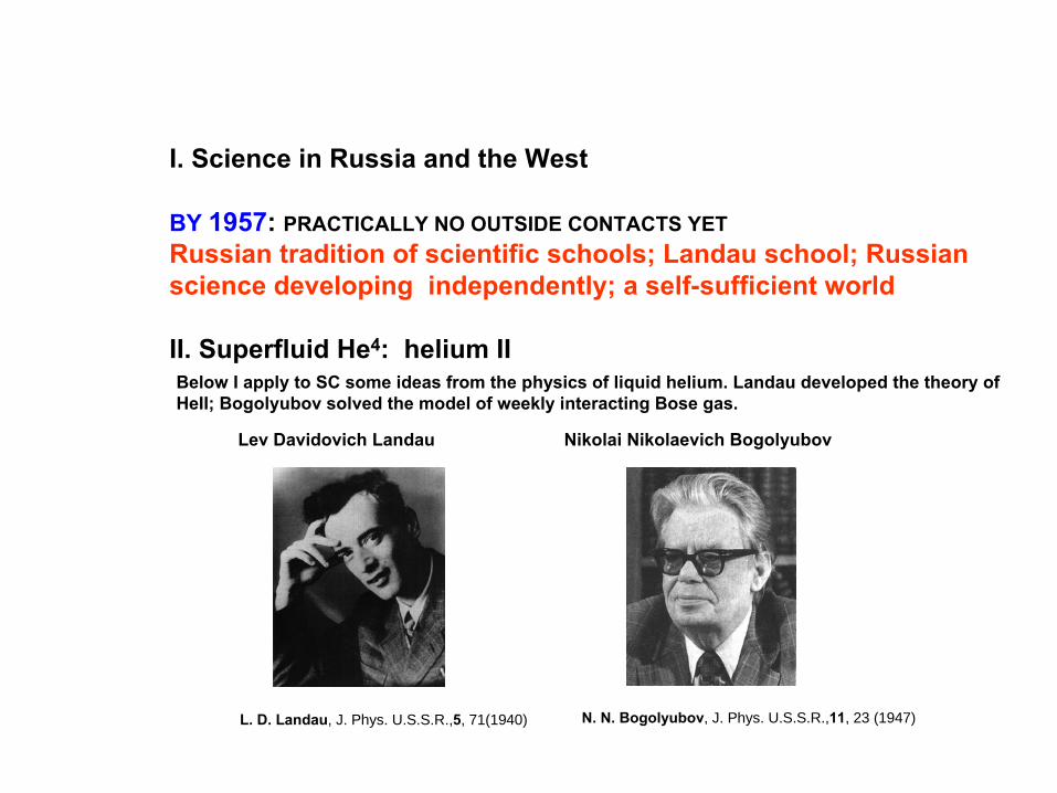
I. Science in Russia and the West

BY 1957: PRACTICALLY NO OUTSIDE CONTACTS YETRussian tradition of scientific schools;

Landau school; Russianscience developing independently; a self-sufficient world

II. Superfluid

He4: helium II

Lev Davidovich

Landau Nikolai Nikolaevich

Bogolyubov

L. D. Landau, J. Phys. U.S.S.R.,5, 71(1940) N. N. Bogolyubov, J. Phys. U.S.S.R.,11, 23 (1947)

Below I apply to SC some ideas from the physics of liquid helium. Landau developed the theory of HeII; Bogolyubov

solved the model of weekly interacting Bose gas.

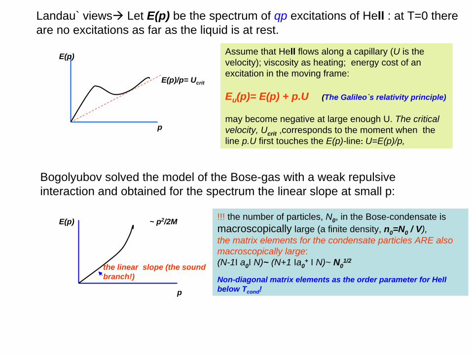
Landau` views Let E(p) be the spectrum of qp excitations of HeIl : at T=0 there are no excitations as far as the liquid is at rest.

E(p)

p

E(p)/p= Ucrit

Assume that HeII

flows along a capillary (U is the velocity); viscosity as heating; energy cost of an excitation in the moving frame:

Eu (p)= E(p) + p.U (The Galileo`s relativity principle)

may become negative at large enough U. The critical velocity, Ucrit ,corresponds to the moment when the line p.U first touches the E(p)-line: U=E(p)/p,

Bogolyubov solved the model of the Bose-gas with a weak repulsive interaction and obtained for the spectrum the linear slope at small p:

E(p)

p

~ p2/2M

the linear slope (the sound branch!)

!!! the number of particles, N0 , in the Bose-condensate is macroscopically large (a finite density, n0 =N0 / V), the matrix elements for the condensate particles ARE also macroscopically large:(N-1I a0 I N)~ (N+1 Ia0

+ I N)~ N01/2

Non-diagonal matrix elements as the order parameter for HeII below Tcond !

III. The BCS –ideas recognized in Russiaa)

The gapped spectrum [Landau criterion!]; The retarded e-ph attraction [J. Bardeen and D. Pines, 1955]

b)

Cooper instability as the qualitative idea phenomenon, capable

to explain why SC is sowidespread among metals, and why Tc is low [ the Cooper logarithm/exponent for Tc!]

c)

Strong anisotropy of the Fermi surfaces in metals no “great expectations” as to the experiment ( actually, as we know, the agreement was remarkable good for the isotropic model! [the Hebel-Slichter peak, 1959])

d)

The theory's consistency and beauty:Bogolyubov: the canonical transformation, variation of the Free Energy expressed in new qp for clean SC Gor'kov: formulation in terms of Quantum Fields Theory (diagrammatic approach), general

IV. Landau seminar

My interests: my thesis(1955) in Quantum Electrodynamics of scalar mesons; Hydrodynamics; HeIIBogolyubov announces his SC theory and is invited to talk at the

Landau Seminar (October 1957)Landau's refuses to understand the ad hoc “principle of compensation of the most dangerous

diagrams”, insists on the physics behind itExhausted N. N. finally gives up and produces the Leon Cooper's paperI realize that it is about a new bosonic

degree of freedom that appears below Tc

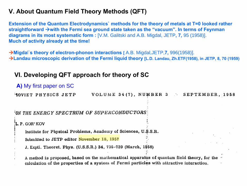
V. About Quantum Field Theory Methods (QFT)

Extension of the Quantum Electrodynamics` methods for the theory

of metals at T=0 looked rather straightforward with the Fermi sea ground state taken as the “vacuum”. In terms of Feynman diagrams in its most systematic form : [V.M. Galitski and A.B. Migdal, JETP, 7, 95 (1958)].Much of activity already at the time!

Migdal`s theory of electron-phonon interactions [ A.B. Migdal,JETP,7, 996(1958)].Landau microscopic derivation of the Fermi liquid theory [L.D. Landau, Zh.ETF(1958), in JETP, 8, 70 (1959)

VI. Developing QFT approach for theory of SC

A) My first paper on SC

The model (BCS) Hamiltonian:

By making use of the commutation relations for the field operators:[ x=(t,x) ]

one obtains equations ofmotion:

apply them to the x=(t,r) argument of the Green function:

products of four field operators appear, needed to be decoupled

for simplicity the interaction between particles was taken into account insofar as it enters into formation of the bound pairs!

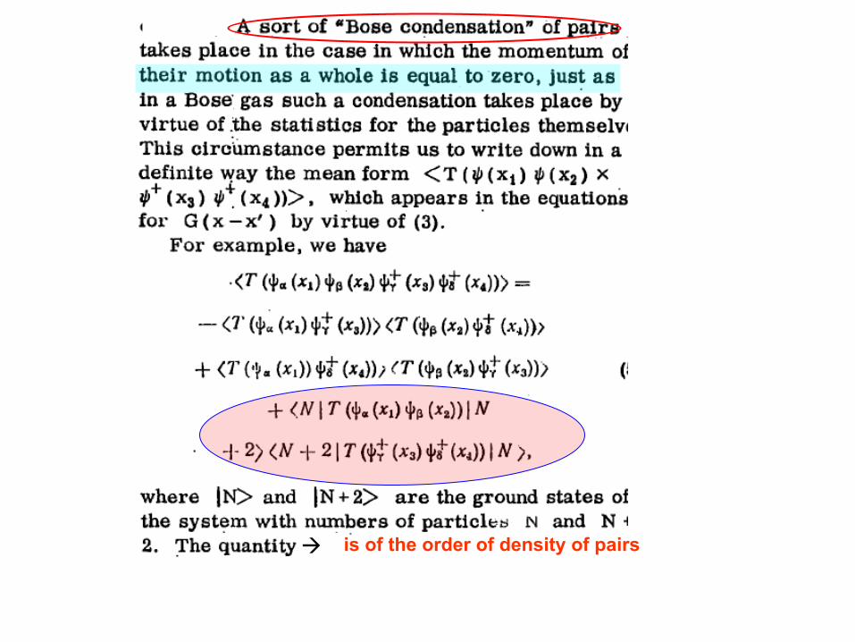
is of the order of density of pairs

To account for the non-diagonal character, take the time derivative of an operator:

one arrives at

[ Note the Josephson exponential factor!]

and to the equations for all Green functions:

Notations for the anomalous functions mean, for instance:

the exponent can be removed by changing variables from N to the chemical potential

F+ F+ F

self-consistency for :=gF(0+) = g

yiI σ̂ˆ −≡

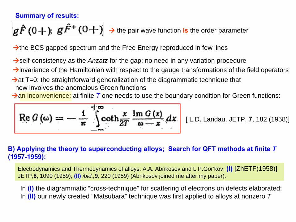
Summary of results:

; the pair wave function is the order parameter

self-consistency as the Anzatz for the gap; no need in any variation procedure

the BCS gapped spectrum and the Free Energy reproduced in few lines

invariance of the Hamiltonian with respect to the gauge transformations of the field operatorsat T=0: the straightforward generalization of the diagrammatic technique that

now involves the anomalous Green functionsan inconvenience: at finite T one needs to use the boundary condition for Green functions:

[ L.D. Landau, JETP, 7, 182 (1958)]

B) Applying the theory to superconducting alloys; Search for QFT methods at finite T (1957-1959):

Electrodynamics and Thermodynamics of alloys: A.A. Abrikosov and L.P.Gor’kov, (I) [ZhETF(1958)] JETP,8, 1090 (1959); (II) ibid.,9, 220 (1959) (Abrikosov joined me after my paper).

In (I) the diagrammatic “cross-technique” for scattering of electrons on defects elaborated; In (II) our newly created “Matsubara” technique was first applied to alloys at nonzero T

All the Green functions, including the anomalous (F, F+), after averaging over impurities:

F(t-t’,R); F+(t-t’,R) F(t-t’,R) exp(-R/l); F+(t-t’,R) exp(-R/l)

(l- the mean free path). The “gap” is proportional to F,F+ at R=0 !in the isotropic model ordinary defects do not affect Tc and thermodynamics“the Anderson Theorem”- [also P.W. Anderson, J. Phys.Chem. Solids, 11,26 (1959)]

C) QFT methods at non-zero T: the thermodynamic technique

))(ˆexp(ˆ)(ˆ int dttHiTS t ∫−=∞+∞

∞−

T=0: Finite T:

)/1(ˆ]ˆˆ

exp[]ˆˆ

exp[ 0 TST

HNT

HN×

−=

− μμ

>∞<>∞′ΨΨ<−

=′+

)(ˆ)(ˆ)(ˆ)(ˆ(ˆ),(

SSxxTixxG

))(ˆexp(ˆ)/1(ˆ/1

0int ττ

τdHTTS

T

∫−=

>><<>>ΨΨ<<

−=+

SSTG ˆˆ)2)(ˆ)1(ˆ(ˆ)2,1(

[T.Matsubara, Prog. Theor.Phys., 14,351, (1955)] found the formal analogy

Diagrammatic technique: the Fourier integrals(t,r) ),( pω

A.A.Abrikosov, L.P. Gor`kov and I.E. Dzyaloshinskii, JETP,9,636(1959)[1958] Imaginary frequency;Fourier series and the analytical continuation from the imaginary axis:

Among the first results for SC alloys:

)(ˆ])ˆˆ(exp[])ˆˆ(exp[ 0 tStNHitNHi ×−−=−− μμ

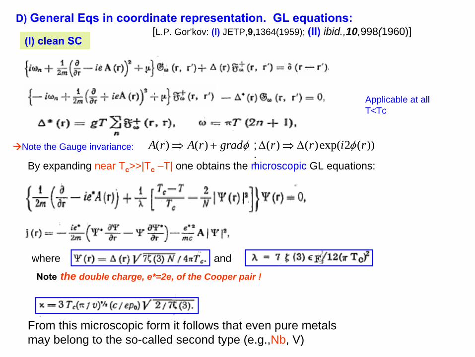
D) General Eqs

in coordinate representation. GL equations:[L.P. Gor’kov: (I)

JETP,9,1364(1959); (II) ibid.,10,998(1960)]

Note the Gauge invariance: φgradrArA +⇒ )()( ))(2exp()()( rirr φΔ⇒Δ

(I) clean SC

By expanding near Tc

>>|Tc

–T| one obtains the microscopic GL equations:

where

Note

the double charge, e*=2e, of the Cooper pair !

From this microscopic form it follows that even pure metalsmay belong to the so-called second type (e.g.,Nb, V)

and

; ;

Applicable at allT<Tc

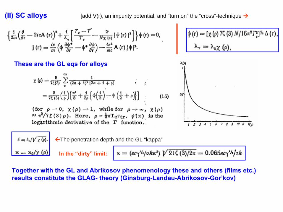
(II) SC alloys [add V(r), an impurity potential, and “turn on” the “cross”-technique

In the “dirty”

limit:

Together with the GL and Abrikosov

phenomenology these and others (films etc.) results constitute the GLAG-

theory (Ginsburg-Landau-Abrikosov-Gor’kov)

The penetration depth and the GL “kappa”

These are the GL eqs

for alloys

(III) Paramagnetic Alloys and Gapless SC [ A.A. Abrikosov and L.P. Gor’kov, JETP,12, 1243(1960)]

I soon noticed that the Cooper instability could be affected by some impurities or an anisotropy

x x>

>

x

x

>

>

+∆ ∆

SppVppV .ˆ)(~)( σ×′−⇒′−

The two types of diagrams cancel each other for ordinary impurities in the isotropic case[“the Anderson theorem”!], but they do not if the two averages differ!

the time-reversal symmetry is broken!We obtained for Tc

)21()

21()/ln( 0 ψ

τψ −+=

sccc T

hTT )(/)()( xxx ΓΓ′=ψ( )

Tc decreases to zero value at

However the gap in the energy spectrum closes first!22

1 0Δ≡=γ

πτ

co

scrit

T

2/33/23/2

0

4/

0 ])/1()[( se τω π −Δ= −

(p) (p`)

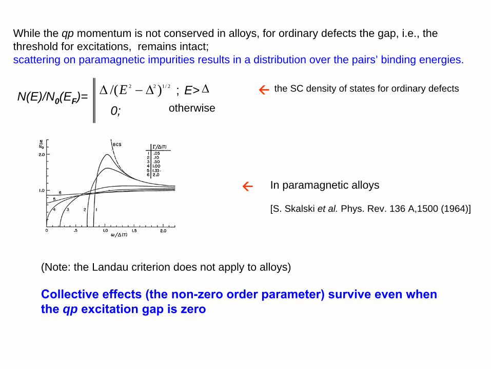
While the qp momentum is not conserved in alloys, for ordinary defects the gap, i.e., the threshold for excitations, remains intact; scattering on paramagnetic impurities results in a distribution over the pairs’ binding energies.

N(E)/N0 (EF )=2/122 )/( Δ−Δ E E>Δ;

0; otherwise

the SC density of states for ordinary defects

In paramagnetic alloys

[S. Skalski et al. Phys. Rev. 136 A,1500 (1964)]

(Note: the Landau criterion does not apply to alloys)

Collective effects (the non-zero order parameter) survive even when the qp excitation gap is zero

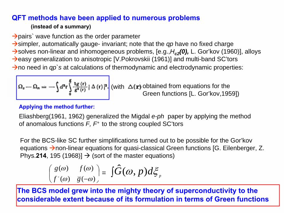
QFT methods have been applied to numerous problems

pairs` wave function as the order parametersimpler, automatically gauge- invariant; note that the qp have no fixed charge solves non-linear and inhomogeneous problems, [e.g.,Hc2(0), L. Gor’kov (1960)], alloyseasy generalization to anisotropic [V.Pokrovskii (1961)] and multi-band SC’torsno need in qp`s at calculations of thermodynamic and electrodynamic properties:

(with obtained from equations for the Green functions [L. Gor’kov,1959])

Eliashberg(1961, 1962) generalized the Migdal e-ph paper by applying the method of anomalous functions F, F+ to the strong coupled SC’tors

For the BCS-like SC further simplifications turned out to be possible for the Gor’kov equations non-linear equations for quasi-classical Green functions [G. Eilenberger, Z. Phys.214, 195 (1968)] (sort of the master equations)

⎟⎠

⎞⎜⎝

⎛−+ )()(

)()(ωωωω

gffg

= ∫ pdpG ξω ),(ˆ

The BCS model grew into the mighty theory of superconductivity to the considerable extent because of its formulation in terms of Green

functions

(instead of a summary)

Applying the method further: