be a man or become a nurse: comparing gender ... · pdf filewissenschaftszentrum berlin...
TRANSCRIPT
WZB Berlin Social Science Center Research Area Markets and Choice Research Unit Market Behavior
Put your Research Area and Unit
Dorothea Kübler Julia Schmid Robert Stüber Be a Man or Become a Nurse: Comparing Gender Discrimination by Employers across a Wide Variety of Professions
Discussion Paper
SP II 2017–201 April 2017
Wissenschaftszentrum Berlin für Sozialforschung gGmbH Reichpietschufer 50 10785 Berlin Germany www.wzb.eu
Dorothea Kübler, Julia Schmid, Robert Stüber Be a Man or Become a Nurse: Comparing Gender Discrimination by Employers across a Wide Variety of Professions
Affiliation of the authors:
Dorothea Kübler WZB Berlin Social Science Center & TU Berlin
Julia Schmid DIW
Robert Stüber BDPEMS & WZB Belin Social Science Center
Copyright remains with the author(s).
Discussion papers of the WZB serve to disseminate the research results of work in progress prior to publication to encourage the exchange of ideas and academic debate. Inclusion of a paper in the discussion paper series does not constitute publication and should not limit publication in any other venue. The discussion papers published by the WZB represent the views of the respective author(s) and not of the institute as a whole.
Wissenschaftszentrum Berlin für Sozialforschung gGmbH Reichpietschufer 50 10785 Berlin Germany www.wzb.eu
Abstract
Be a Man or Become a Nurse: Comparing Gender Discrimination by Employers across a Wide Variety of Professions
by Dorothea Kübler, Julia Schmid and Robert Stüber*
We investigate gender discrimination and its variation between firms, occupations, and industries with a factorial survey design (vignette study) for a large sample of German firms. Short CVs of fictitious applicants are presented to human resource managers who indicate the likelihood of the applicants being invited to the next step of the hiring process. We observe that women are evaluated worse than men on average, controlling for all other attributes of the CV, i.e., school grades, age, information about activities since leaving school, parents' occupations etc. Discrimination against women varies across industries and occupations, and is strongest for occupations with lower educational requirements and of lower occupational status. Women receive worse evaluations when applying for male-dominated occupations. Overall, the share of women in an occupation explains more of the difference in evaluations than any other occupation- or firm-related variable.
Keywords: Gender discrimination, hiring decisions, vignette study
JEL classification: C99; J71
* E-mail: [email protected], [email protected], [email protected].
We would like to thank Heike Solga and Paula Protsch for their collaboration and fruitful discussions, the BIBB (Federal Institute of Vocational Education and Training) which made the study possible, and also Katrin Auspurg who helped us with the selection of the vignettes. We also would like to thank Bernd Fitzenberger, Kristina Strohmaier and Marina Töpfer for their comments. We are grateful to Thu-Ha Nguyen, Michaela Zwiebel, Sajoscha Engelhardt, and Manuela Ludwig for their assistance. The paper has benefited from seminar participants at the Humboldt University of Berlin. Financial support from CRC TR190 is gratefully acknowledged. All remaining errors are our own.

1 Introduction
Labor market outcomes for men and women di�er along many dimensions, such as wages earned
and the number of working hours. While di�erent trajectories in the labor market may be due to
di�erences unfolding in the life course, such as asymmetries in the e�ects of having children (see
Kleven et al., 2017), we focus on the �rst stage of people's careers, namely their entry into the
labor market. We ask how young women and men fare right after leaving school when applying
for their �rst job. Since girls, on average, do at least as well in school as boys, it can be expected
that their chances of getting a job after school should be at least as good as those of young men.
We ask whether this is the case by looking at the employment probabilities of men and women
early in the career.
We aim to make two contributions, one substantive on discrimination and one methodological.
First, our study investigates whether �rms from many di�erent industries discriminate by gender
when hiring in the entry-level labor market. By gender discrimination we mean that men and
women who are equal with respect to all observable productivity-related characteristics are treated
di�erently by employers.1 While there are many studies that leave no doubt about the existence of
discrimination in certain professions, a more comprehensive picture of the labor market is missing
in order to establish in which segments of the labor market and for which professions discrimination
is observed.
Regarding the methodology, we conducted a survey experiment based on vignettes consisting of
the CVs of �ctitious applicants. The respondents of the survey were asked to evaluate the �ctitious
applicants as if they had applied for an apprenticeship position in the �rm. This method, which
to our knowledge has not been used to investigate labor market discrimination, has a number of
advantages, and it complements the use of observational data and �eld experiments. First, we are
able to estimate the causal e�ect of being female on our outcome variable (the evaluations). By
varying the di�erent dimensions of the vignette (items on the CV), we can analyze how gender
discrimination varies with the quality of an application. This, together with our outcome variable
being non-binary, allows us to address Heckman and Siegelman's critique of �eld experiments
that do not vary the quality of the applicant. They point out that if the variance of unobserved
productivity characteristics di�ers between men and women, taking a snapshot at one quality
level of applicants (as most �eld experiments do) can generate a biased measure of discrimination.
Moreover, our survey was conducted with a large sample of German �rms hiring apprentices in 126
di�erent professions, which permits us to investigate the �rm- and occupation-speci�c determinants
of gender discrimination, using an experimental design.
We focus on the market for apprenticeships, which is the main entry-level labor market for
young Germans below the level of tertiary education. More than 60% of all school-leavers start an
1This encompasses taste-based and statistical discrimination. Note that statistical discrimination is seen asacceptable in some contexts (young drivers have to pay more for car insurance, for example), while it is consideredas unacceptable or illegal in other contexts, such as gender- or race-based hiring decisions.
2

apprenticeship, and more than half of the apprentices remain employed by the �rm that trained
them.2 The hiring procedures for apprentices are similar to those for other employees. The market
for apprenticeships is competitive in that a number of applicants do not get a job in their desired
profession, and many applicants remain without a job every year. At the same time many slots
remain un�lled due to strong regional and occupational di�erences.
We �nd economically substantial and statistically signi�cant discrimination against women.
The penalty for being female is as large as the e�ect of having a grade point average that is
worse by one grade.3 In contrast, we do not observe any discrimination based on an applicant's
socioeconomic background. Furthermore, the amount of discrimination varies by industry. In line
with prior research, it also matters whether an occupation is predominantly female or male, with
women being signi�cantly less attractive than men when applying for male-dominated occupations.
We do not �nd evidence of discrimination against men in female-dominated occupations though.
We also �nd no evidence of discrimination if the labor market is very tight. On the other hand,
the size of the �rm (as measured by the number of employees or the number of apprentices) and
the degree of professionalization of the recruitment process do not matter as moderators of gender
discrimination.
Prior research suggests that women experience discrimination in high-status occupations. We
consider a number of variables that are indicative of the status of a profession. First, we study
whether the average salary of a profession moderates discrimination. Then we consider the typical
school-leaving quali�cation required for the profession. Clearly, the average salary of a profession
and its required education level may in�uence gender discrimination for reasons other than status
concerns, but both are correlated with indices of occupational status developed in the literature.
We �nally investigate how these indices of occupational status in�uence discrimination. Women
fare especially worse than men in professions requiring the lowest school degree and for professions
with a low social status, according to the status indices. The average wage of a profession has no
systematic impact on gender di�erences in evaluations.
After providing evidence on the correlation between the occupations and industry characteris-
tics with gender discrimination, we determine which of the variables can explain discrimination.
The experimental literature has studied the role of the share of women in a profession, but the
existing studies have looked at a limited number of professions and are unable to control for the
variation of the status of a profession (for example, secretaries as typically female and engineers as
typically male occupations). We are able to disentangle the di�erent characteristics of the profes-
sions and provide evidence of the ceteris-paribus e�ect of each of the potential moderator variables
on gender discrimination.
Our main �nding is that the share of women in a profession explains most of the di�erence
in evaluations. All other �rm- and occupation-speci�c variables cannot explain the discrimination
2See BIBB (2012) and BMBF (2012), respectively.3German school grades range from 1 (best) to 6 (worst) where 4 is the passing grade.
3

observed. These results are novel because they are derived from a large sample of �rms, allowing
us to control for many possible moderators.
2 Literature and research questions
This study relates to the literature on discrimination in the labor market as well as to method-
ological contributions regarding the identi�cation of discrimination. We discuss these two strands
of the literature in turn and explain how our study contributes to them.
Discrimination in the labor market
Traditionally, labor economists have applied regression-based methods to observational data in
order to measure (gender) discrimination in the labor market (see Altonji and Blank, 1999, for
an overview). Analyzing both the di�erence in wages and participation rates, there is evidence of
gender discrimination in the labor market. However, this literature su�ers from a number of draw-
backs (Azmat and Petrongolo, 2014). One important problem is the possibility that discrimination
is overestimated, since it is the residual after controlling for observable di�erences in productiv-
ity where these productivity di�erences might be insu�ciently measured. For this reason, many
researchers have conducted �eld experiments to study discrimination in the labor market.4
In the experiments, call-back rates, invitations to job interviews or job o�ers are compared
between arti�cial applicants that are similar with respect to their characteristics but di�er, e.g.,
with respect to race, ethnicity, or sex. Hence, applicants are equal with respect to their observ-
able productivity and di�erences in outcomes are interpreted as re�ecting discrimination.5 This
literature found evidence consistent with labor market discrimination against black people in the
United States (Bertrand and Mullainathan, 2004), against Turkish immigrants in Germany (Kaas
and Manger, 2011), and against young women for high-skilled jobs in France (Petit, 2007), among
many other groups.
Gender discrimination may be driven by existing di�erences in the share of women and men
in an occupation. One possible reason is that the prevalence of one gender causes stereotyping,
resulting in a more favorable outcome for the dominant gender in the occupation (Booth and
Leigh, 2010). Relatedly, psychological evidence suggests that individuals working in a job where
one gender is prevalent think that success in this job requires characteristics typical of that gen-
der (Schein, 1973). This in�uence of the gender composition of an occupation on discrimination
4Alternative approaches based on observational data were also developed, see e.g., Bayard et al. (2003). There arealso laboratory studies on the e�ect of gender on hiring recommendations. In these studies students' or recruiters'are asked to rate the employment suitability of applicants, while applicant gender is varied. These studies �ndmixed evidence but Olian et al. (1988) conclude from their meta-analysis that there is only little evidence of genderdiscrimination.
5These �eld studies take on two di�erent forms. In the case of audit studies, applicants trained to act alike applyfor jobs, while correspondence studies use written or online applications.
4

has received some attention in the literature. Table 1 shows studies that compare occupations
with a varying share of female employees. Levinson (1975) and Riach and Rich (2006) both �nd
discrimination against men in female-dominated occupations and discrimination against women
in male-dominated occupations while in both studies the discrimination against men in female-
dominated occupations is more pronounced. Hence, gender discrimination seems to di�er across
jobs with di�erent shares of female employees. This is especially interesting since the two stud-
ies di�er with respect to method, location, time, and occupations considered. In addition, in
their correspondence study conducted in the UK, Riach and Rich (2006) also �nd discrimination
against males for accountants and computer programmers � two occupations that they classify
as gender-neutral. These �ndings contrast with the results of Riach and Rich (1987) based on
a correspondence study conducted in Australia where discrimination against women is found in
some (computer programmer and gardener) but not all of the male-dominated occupations. No
discrimination against men is found in the female-dominated profession of clerical worker.
Motivated by these studies, Booth and Leigh (2010) consider female-dominated occupations
with a varying gender ratio. They �nd signi�cant discrimination against men for the entire sample
and also for the two occupations with a larger share of women (data-entry and waitsta�), but no
signi�cant discrimination for the two occupations with a lower share of women (customer service
and sales). Note that these two latter occupations are still female-dominated, only to a lower
degree. Weichselbaumer (2004) compares interview invitations between a feminine woman, a more
masculine woman, and a man in Austria. The women's gender identity is conveyed via di�erent
items such as the hobbies and the picture in the CV. Weichselbaumer �nds discrimination against
both types of women for one of the two occupations that are male-dominated, but not for the
other. She also �nds discrimination against men (and in favor of masculine and feminine women)
for the strongly female-dominated occupation of a secretarial assistant. No statistically signi�cant
di�erences between the three applicant types are found for the female-dominated occupation of an
accountant.
Given this evidence, there seems to be a relationship between gender composition and discrim-
ination that deserves closer attention.6 Our sample allows us to compare occupations with a share
of female employers between almost 0 and 100 percent, thereby providing evidence over the entire
range of gender ratios. Moreover, we employ two di�erent measures of the gender ratio. Like most
previous studies, we base one of our measures on the national average for each apprenticeship
occupation. Our second measure of gender dominance is the respondents' self-reported share of
female employees in the apprenticeship occupation in the �rm.
It has been argued that discrimination is stronger in occupations of higher status and in jobs
that are more senior (Riach and Rich, 2002; Azmat and Petrongolo, 2004). This claim is based,
in part, on the �ndings for occupations with di�erent shares of female employees. Also, the
6Early evidence from psychology on the in�uence of an occupation's gender-type on discrimination is mixed(e.g., Cohen and Bunker, 1975, Muchinsky and Harris, 1977).
5

Table1:
Field
experimentson
gender
discrimination:
thee�ectsof
thegender
ratioandstatus
StudyandMethod
LocationandTime
Occupations
Measure
Finding
Genderratio:
Booth
andLeigh(2010)
Brisbane,Melbourne,
Data-entrist(f,85%),waiters(f,80%),
Australianaverage
Discriminationagainstmen
fordata-entryand
(CS)
Sydney,Australia
customer
serviceem
ployees(f,68%)
(AustralianBureau
waitsta�,nodiscriminationforcustomer
serviceand
(2007)
salesm
an(f,69%)
ofStatistics2007)
andsales
Riach
andRich(2006)
England
Chartered
Accountants(n,31%),
UKaverage
Discriminationagainstwomen
in(m
)occupations
(CS)
(2003)
computeranalysts/
programmers(n,21%),
(O�ce
ofNational
andagainstmen
in(f)and(n)occupations,
engineers(m
,5%),secretaries
(f,97%)
Statistics2003)
discriminationagainstmen
more
pronounced
Weichselbaumer
(2004)
Vienna,Austria
Network
technicians(m
,13%),computer
Austrianaverage
Discriminationagainstmasculineandfeminine
(CS)
(1998-1999)
programmers(m
,13%),accountants(f,77%),
(AustrianCensus1991)
women
fornetwork
techniciansandagainstmen
for
secretaries
(f,97%)
secretaries,forothersnodiscriminationbetween
men,femininewomen,andmasculinewomen
Riach
andRich(1987)
Victoria,Australia
Managem
entAccountants(m
,9%),
Victorianaverage
Discriminationagainstwomen
forcomputer
(CS)
(1983-1986)
computerprogrammers(m
,23%),analyst
(AustralianBureau
programmersandgardeners,forothersno
programmers(m
,23%),computer
ofStatistics1981)
discrimination
operators(N
I),industrialrelationso�cers(N
I),
clericalworkers(f,68%),gardeners(m
,13%)
Levinson(1975)
Atlanta,USA
Mostly
secretaries/receptionists(f),
NI
Discriminationagainstmen
in(f)occupations
(AS)
(1974)
mostly
security
guards/
o�cers/
andagainstwomen
in(m
)occupations,
(telephoneinquiries)
managers/
skilledworkers(m
)discriminationagainstmen
more
pronounced
Status:
Neumark
etal.(1996)
Philadelphia,USA
Waiters(H
igh,
Price
level
Discriminationagainstwomen
inhigh-price
(AS)
(1994)
medium
andlowprice/earnings)
restaurants(jobo�fersandinterviewinvitations)
(in-personinquiries)
andagainstmen
inlow-price
restaurants(only
w.r.t.
jobo�ers),nodiscriminationin
medium-price
restaurants
Firth
(1982)
England
Articledclerksandquali�ed
accountants
NI
Discriminationagainstwomen
forquali�ed
(CS)
(1978)
workingforprofessionalaccounting�rm
saccountantsworkingin
industry
and�nancialjobs,
(noncareer
jobs),unquali�ed
personnel,
nodiscriminationforallother
professions
quali�ed
accountantsworkingin
industry
and�nancialjobs(career
jobs)
Note:Thetableshow
spublicationsthatcompare
discriminationacrossoccupationswithdi�erentsharesoffemaleem
ployeesaswellaspublicationsfocusingonoccupationswithdi�erent
socialstatus.
CSrefers
toacorrespondence
studywhileASindicatesanauditstudy.
NIabbreviates"notindicated".(f)meansthattheauthors
classifytheoccupationasfemale
dominated,(m
)meansthatthey
classifyanoccupationasmaledominated,and(n)meansthey
classifyanoccupationasgender
neutral,wherethepercentagerefersto
theratiooffemale
employees.Measure
refersto
themeasure
onwhichtheauthorsbase
theircategorization.
6

�ndings of Neumark et al. (1996) suggest that discrimination against women is higher for high-
status occupations and lower, or potentially reversed, for low-status occupations (see also Table
1). The results of Firth (1982) can be interpreted as pointing in the same direction, although he
�nds discrimination against women only in two out of the three high-status professions. Equally,
Riach and Rich (1987) note in their study that one of the two occupations for which they �nd
discrimination is a high-status occupation, while the other is not. Unfortunately, not all of the
studies report the measure of status on which they base their categorization. Given the few
studies and the mixed results, the hypothesis that discrimination is more pronounced in high-
status occupations calls for further scrutiny.
Larger �rms have been found to discriminate less between men and women (Engels, 2015; Akar
et al., 2014). One possible explanation is that evaluating larger groups of applicants leads to de-
cisions that are less a�ected by group stereotypes (Bohnet et al., 2016). Another possible channel
is that a more formalized and professional recruitment procedure might counteract gender dis-
crimination. In addition, discrimination should be smaller if the total supply of applicants is small
compared to the demand. Finally, parental background (the parents' education and profession) has
been shown to in�uence the children's educational choices and achievements (Dustmann, 2004).
Researchers have also found a high persistence of occupations between generations (Knoll et al.,
forthcoming; Jonsson et al. 2009). We can study whether the employers' evaluations contribute
to these outcomes by studying the e�ect of the mother and father's profession on an applicant's
evaluation.
Identifying discrimination
Just as �eld experiments, the vignette design allows us to observe the causal e�ect on the evaluation
of being female or male. However, Heckman (1998) and Heckman and Siegelman (1993) have
questioned the validity of �eld experiments that use correspondence methods.7 Two points of their
criticism remain valid for many recent �eld experiments, and we discuss that the factorial survey
method can address one of them. Finally, we point out additional methodological bene�ts of our
research design.
First, even if a researcher conducting a correspondence study is successful in making the ap-
plicants of the two groups under consideration equal with respect to the observed productivity
characteristics, that is, the characteristics mentioned in the written application, a necessary as-
sumption to identify discrimination is the equality of the average unobserved productivity-related
factors of the two groups.8 There should not be any di�erences in the mean of unobserved char-
7They have also criticized audit studies on the grounds that the testers acting as job applicants can in�uence theresults. Often, the testers are not blind to the research question, thereby potentially causing experimenter demande�ects. Note that correspondence tests relying on written applications do not su�er from this problem. They havealso argued that any detection of discrimination in these studies only indicates that the average employer (and notthe marginal employer) discriminates.
8Heckman and Siegelman make their argument for the case where unobserved productivity-related factors arefactors that are unobservable to the researcher but visible to the employer and are taken into account in the
7
acteristics across the two groups. Otherwise, di�erences in outcomes might be due to di�erences
in these unobservable productivity characteristics or due to group membership alone. Without
assuming or ensuring that unobserved productivity factors are equal for both groups, researchers
are not able to distinguish between the two.
The factorial survey method has in common with �eld experiments that we cannot di�erentiate
between discrimination arising due to di�erences in the unobserved productivity characteristics or
due to group membership alone. More generally, it is possible that the employers' estimates of the
mean group productivity di�er between men and women and that any di�erences in outcomes are
due to these di�erent expectations of employers upon seeing a male or female applicant. Thus, we
can only identify discrimination that may be taste-based, statistical, or both.9
The second point raised by Heckman and Seligman concerns the variance of the unobserved
productivity variable. Even if the mean unobserved productivity does not di�er between the two
groups under consideration, di�erences in the variance of the unobserved productivity between the
groups can cause evidence of discrimination to be biased if the employers' hiring decisions are based
on a cut-o� rule (see Neumark (2012) for a detailed discussion). To see this, assume that both the
average observed and unobserved productivity are equal across the two groups under consideration.
Further assume that the variance of the unobserved productivity is higher for one group, say for
women. If the researcher sets the observed productivity-related characteristics in the written
application to a low value, and if the variance of unobserved characteristics is higher for women,
women have a higher probability of being invited to an interview than men. In contrast, if the
researcher designs applications with a high quality of observable productivity characteristics, the
group with the lower variance in unobserved characteristics will receive more interview invitations.
Thus, the observed discrimination can be an artefact of the study design.
Neumark (2012) proposes a statistical method to identify the level of discrimination despite this
second problem. If a study has enough variation in the observable productivity characteristics, a
heteroskedastic probit model can be used to infer the ratio of standard deviations of the unobserved
productivity characteristics between the two groups and to back out discrimination. This procedure
requires to assume that the coe�cients on all observable applicant characteristics do not vary
between the two groups under consideration. Neumark (2012) discusses examples for which this
assumption is violated, e.g., if the productivity e�ects of schooling di�er between two groups.10
Our estimate of discrimination between men and women is robust to Heckman and Seligman's
unobserved variance critique for the following reasons. The estimate of discrimination is based
on a 10-point evaluation scale and not on a cut-o� value such as a binary invitation decision.
hiring decisions, while typically statistical discrimination refers to a situation where employers cannot observe anapplicant's true productivity and hence partially rely on the average productivity of the group to which an applicantbelongs (see below).
9For lab and lab-in-the-�eld experimental evidence regarding taste-based discrimination see Fershtman andGneezy (2001) and List (2004).
10The advantage of the assumption is that it has testable implications.
8

As long as our 10-point scale fully covers all evaluations the employers want to make, which
we deem reasonable, the employers' evaluations of the applicants are linear in productivity and
our estimate of discrimination is robust to di�erences in the variance of unobserved productivity
components between men and women.11 However, even if this assumption was invalid, di�erences
in the variance of unobserved productivity components between men and women are unlikely to
cause our estimate to be biased for the following reason. As suggested in Neumark (2012), one
way to address the unobserved-variance critique is to vary the level of applicant characteristics
relevant to the hiring decision. If discrimination is found for di�erent levels of the characteristics,
the results cannot be due to di�erences in the variance of unobserved characteristics. The design
of our vignette study allows us to simultaneously vary several applicant characteristics such as the
duration of unemployment after leaving school or the average school grade. Signi�cant coe�cients
show that these characteristics have an e�ect on hiring. Hence, our applicants di�er with respect to
their observable productivity level. In addition, employers from �rms of eight di�erent industries
and 126 occupations evaluate our vignettes.12 As the quality of an applicant depends on the
requirements of the evaluator and on the occupation, we thereby consider a large variation in the
quality of applicants.
Another advantage of the vignette design is that we can test whether Heckman and Siegelman's
unobserved variance critique of �eld studies is warranted. Applicants are evaluated on a range from
1 to 10. If a di�erence in the variance of unobserved productivity components of men and women
(resulting in a di�erence in the variance of productivity) is the reason for the discrimination against
women found in earlier studies, this must be re�ected in the distribution of evaluations. That is,
if the variance of the unobserved productivity is higher for women than for men, we will observe
a higher variance in the evaluations of women than of men.
Finally, the factorial survey design allows us to observe a �ner measure of how applicants are
evaluated. While it seems to be the case that �rms evaluate applicants relative to a standard
when they decide whether or not to invite a candidate to the next step of the recruitment process,
the impact of an application on a candidate's employment probability at the stage at which �eld
studies evaluate employer behavior is not necessarily binary. Although employers ultimately de-
cide whether or not to hire a certain applicant, group membership might have an impact on the
employer's evaluation beyond its impact on the call-back rate or the probability of being invited
to an interview. An applicant from a minority might be invited to an interview though she or he
might still be disadvantaged at later stages of the application process. By allowing employers to
submit an evaluation on a scale from 1 to 10, we hope to capture more subtle di�erences between
applicants.
11Note that our estimate of discrimination does not rely on the additional assumptions of Neumark's (2012)approach.
12In contrast, in the usual correspondence study applications are sent out for a small number of occupations (upto seven in the studies we are aware of).
9

Testing for statistical discrimination à la Aigner and Cain (1977)
We can use our dataset to shed some light on the nature of discrimination in our sample by testing
for a certain form of statistical discrimination. In one of the classical models of statistical labor
market discrimination by Aigner and Cain (1977), productivity is unobserved and employers have
to form expectations about a worker's true productivity. The expected productivity of a worker is
given by the weighted average of the mean productivity of the group to which the worker belongs
and a measure of her individual productivity. In other words, since the true productivity is unob-
served, employers rely partly on the group information. The weight on the individual productivity
indicator is de�ned by the variance of the real productivity and the variance of the error when
measuring the productivity indicator instead of the true productivity, and can be interpreted as
the reliability of the productivity indicator. Statistical discrimination can arise due to di�erences
in the average group productivities, but it can also arise due to di�erences in the reliability of
the productivity indicator resulting in a worse signal strength (with average group productivities
being equal). Intuitively, employers put more weight on the individual productivity indicator and
less weight on the group mean for individuals belonging to the group for which the signal is more
informative, which leads to an unequal treatment of equally productive applicants whenever the
individual productivity indicator di�ers from the mean group productivity. For such di�erences
in the reliability of the productivity indicator to arise, it can be assumed that the variance of the
real productivity varies between groups, or that the variance of the real productivity is equivalent
for the two groups but that the indicator is less precise in measuring real productivity.13
Two features of the design of our study enable us to test whether a di�erence in the signal
strength induced by the productivity indicator being less precise in measuring real producitvity
causes statistical discrimination. First, we vary the applicant characteristics quite substantially
and hence expect to observe applicants that are considerably above the average productivity and
applicants that are considerably below average. Second, under the additional assumption that the
share of currently employed female apprentices is the decisive factor that causes the signal strength
to vary, observing the share of currently employed female apprentices for all our employers means
that we observe a proxy for the signal strength. For instance, �rms with a high share of female
employees have a better prior knowledge of the productivity distribution of women and, hence,
the signal emerging from the productivity indicators is more precise. If this reasoning is valid, a
better-than-average woman applying to these �rms should be evaluated better than a man who is
better than average and who has the same observable productivity characteristics. This is because
employers put more weight on the woman's individual signal than on her group signal compared
to a man. In contrast, a worse-than-average woman should be evaluated worse than a worse-
than-average man who has the same observable productivity characteristics. Finally, the reverse
13The former assumption of di�erent variances of real productivity between groups is comparable to Heckmanand Siegelman's unobserved variance critique. Note again, however, that their criticism is based on an observed andan unobserved productivity component, which are both observed by employers, while in Aigner and Cain's modelemployers have to form an expectation.
10

reasoning applies for �rms with a low share of female apprentices. We test whether the evaluations
of men and women are consistent with this form of statistical discrimination.
3 Study design
The vignette study was embedded in an annual panel survey of �rms engaged in apprenticeship
training. In cooperation with the Company Panel on Quali�cation and Competence Development
of the Federal Institute of Vocational Education and Training (BIBB), we included the vignettes as
well as questions concerning the �rms' recruitment procedures in the survey wave of 2014 (BIBB
Training Panel 14). In total, 3,450 �rms participate in the panel. Out of these, we randomly
selected 680 �rms to additionally take part in our factorial survey. About half of our �rms have
less than 100 employees. Some �rms o�er apprenticeships for several professions. We asked them
to evaluate our �ctitious applicants for their most frequent apprenticeship position. Among the
�rms in our survey, the most frequent apprenticeships are in technical professions (53%), followed
by business or administrative professions (35%), and educational or nursing professions (12%).
The respondents of the computer-assisted personal interviews (CAPI) were �rm owners, man-
agers, and employees involved in human resources. They were �rst given a number of questions
regarding the hiring process. Then they were asked to evaluate short descriptions of applicants
(vignettes) for an apprenticeship in the occupation for which their organization trains most people.
Within the vignettes, we varied the applicants' attributes (dimensions). The method, also known
as a factorial survey experiment, embeds randomized treatments in a survey. It allows for study-
ing the relative importance of a number of applicant characteristics simultaneously. Thus, we can
determine which information about the applicant is actually being used. Moreover, it is possible
to measure the in�uence of a single variable and of combinations of variables on the evaluations.
All respondents had to evaluate �ve vignettes, each of them describing a �ctitious applicant, with
respect to whether he or she would reach the next step of the hiring procedure. Answers had to
be provided on a scale from 1 (very unlikely) to 10 (very likely). Overall, we attempted to collect
3,400 evaluations of the �ctitious applicants.
In comparison to correspondence tests, the factorial survey method relies on hypothetical,
not real decisions. Hence, the answers might di�er from actual behavior. Similarly, the answers
might be a�ected by demand e�ects when respondents try to please the interviewer or try to
provide socially acceptable answers.14 In order to limit such concerns with respect to gender as
our main variable of interest, the �ve �ctitious applicants described in the vignettes that every
respondent received from us were of the same gender. Demand e�ects are also minimized by the
fact that respondents were not asked directly, for example, for the role of gender or grades for their
14This might not only bias our baseline �ndings, but also the �ndings of our correlational analysis. For instance,the desire to give socially acceptable answers might be di�erently strong for occupations with a di�erent share offemale apprentices.
11
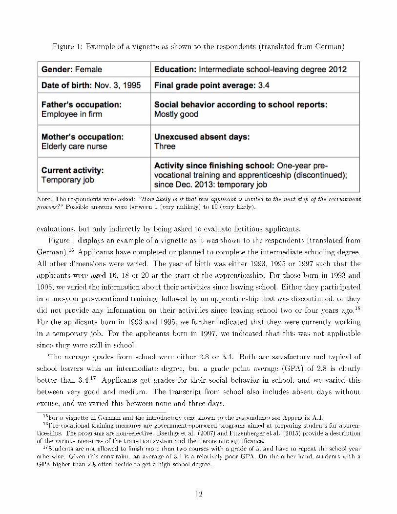
Figure 1: Example of a vignette as shown to the respondents (translated from German)
Note: The respondents were asked: "How likely is it that this applicant is invited to the next step of the recruitment
process?" Possible answers were between 1 (very unlikely) to 10 (very likely).
evaluations, but only indirectly by being asked to evaluate �ctitious applicants.
Figure 1 displays an example of a vignette as it was shown to the respondents (translated from
German).15 Applicants have completed or planned to complete the intermediate schooling degree.
All other dimensions were varied. The year of birth was either 1993, 1995 or 1997 such that the
applicants were aged 16, 18 or 20 at the start of the apprenticeship. For those born in 1993 and
1995, we varied the information about their activities since leaving school. Either they participated
in a one-year pre-vocational training, followed by an apprenticeship that was discontinued, or they
did not provide any information on their activities since leaving school two or four years ago.16
For the applicants born in 1993 and 1995, we further indicated that they were currently working
in a temporary job. For the applicants born in 1997, we indicated that this was not applicable
since they were still in school.
The average grades from school were either 2.8 or 3.4. Both are satisfactory and typical of
school leavers with an intermediate degree, but a grade point average (GPA) of 2.8 is clearly
better than 3.4.17 Applicants get grades for their social behavior in school, and we varied this
between very good and medium. The transcript from school also includes absent days without
excuse, and we varied this between none and three days.
15For a vignette in German and the introductory text shown to the respondents see Appendix A.1.16Pre-vocational training measures are government-sponsored programs aimed at preparing students for appren-
ticeships. The programs are non-selective. Baethge et al. (2007) and Fitzenberger et al. (2015) provide a descriptionof the various measures of the transition system and their economic signi�cance.
17Students are not allowed to �nish more than two courses with a grade of 5, and have to repeat the school yearotherwise. Given this constraint, an average of 3.4 is a relatively poor GPA. On the other hand, students with aGPA higher than 2.8 often decide to get a high school degree.
12

Finally, in order to investigate whether the socio-economic background of the applicant matters,
we chose di�erent professions of the father. He was either a warehouse clerk, an insurance salesman,
a teacher, or an employee in the respective �rm. Many �rms have rules according to which children
of employees automatically pass the �rst selection step, and we therefore expect these applicants
to pass the hurdle with a higher probability. The other three professions di�er with respect to
salaries and educational requirements.18 The mother had one of two professions of similar status,
salary, and required education, namely nursery-school teacher and elderly-care nurse.19
4 Results
Our main dependent variable is the evaluation of the �ctitious applicants on a 10-point scale. The
response rate of the 680 �rms selected for our survey is more than 98% with only 47 out of 3,400
evaluations of �ctitious applicants missing. We exclude from the analysis respondents who indicate
that they do not know the recruitment procedure of their �rm, respondents who state that their
�rm does not have a recruitment procedure, and respondents who report that their �rm does not
review and examine the application documents. Overall, this leaves us with a sample of 3,164
evaluations made by 636 respondents.
The BIBB provides us with sampling weights for our set of �rms to correct for imperfections
of the sample with respect to the full sample of �rms training apprentices in Germany. We
conducted all estimations both with and without the sample weights. Most results are qualitatively
unchanged. We state all results based on the unweighted estimations. However, we also provide
the results using the sampling weights whenever they deviate from the unweighted results with
respect to the signi�cance of an e�ect.
4.1 Is there a gender di�erence in evaluations?
For a �rst impression of the evaluations provided by the respondents, Figure 2 shows the distribu-
tion of evaluations for male and female applicants. Apart from indicating that the respondents use
the full scale of possible evaluations, the �gure also reveals a di�erence in the evaluation of men
and women, with more frequent positive evaluations of men compared to women. Women receive
bad evaluations (1-5) more often than men, while men receive good evaluations (6-10) more often
than women. The bars for the worst (1) and the best evaluation (10) display the largest di�erences
between women and men. For instance, 241 female applicants receive an evaluation of 1, indicat-
ing that an invitation to the next recruitment step is very unlikely, while only 97 male applicants
18In Germany a warehouse clerk earned, on average, between 12.98 and 15.55 Euro per hour in 2014, while ateacher earned 24.78, and an insurance salesman earned between 23.74 and 28.98 Euro (Federal Statistics O�ceDestatis, 2016). Working as a teacher requires a university degree in Germany while insurance brokers and (to alesser degree) warehouse clerks usually complete an apprenticeship.
19Nursery-school teachers earned, on average, between 13.60 and 16.43 Euro in Germany in 2014 while elderly-carenurses earned 14.42 Euro (Federal Statistics O�ce Destatis, 2016).
13

receive this evaluation. Only 137 female applicants receive an evaluation of 10, indicating that the
invitation is very likely, while 213 men receive this evaluation. Male applicants receive an average
evaluation of 6.14 while female applicants receive an average evaluation of 5.21 such that the male
applicants' evaluations are on average 0.93 points better than those of female applicants. This
di�erence in means is signi�cant (t-test, p<0.001).
Figure 2: Evaluation of Fictitious Applicants by Gender
Note: Frequency of each evaluation for male and female applicants.
Our vignettes are chosen such that the applicant characteristics are equal for men and women
in expectation. Thus, if the randomization worked, the observed mean discrimination against
women should be unchanged if we regress the evaluations on a gender dummy and all other vi-
gnette dimensions (applicant's age, mother and father's occupation, average grade, social behavior,
number of absent days unexcused, and the gap after school). Since one respondent evaluated �ve
vignettes, we use a random-e�ects (RE) estimation and take into account the dependencies of the
answers at the level of the respondents (�rms).20 We �nd that women are evaluated 0.90 points
worse than men, which is highly statistically signi�cant (see Table 2). It is also economically rele-
vant: Supposing a linear e�ect of an applicant's GPA on the evaluation, being a man instead of a
woman makes up for almost one grade level from school. The only vignette dimension that has a
stronger impact on the respondents' evaluations is a four-year gap after school. Since applications
from older applicants indicate that they had issues at their career entry, it is not surprising that
this variable is relevant for the employers' evaluations. Besides, Table 2 indicates that several
other applicant characteristics matter for the employers' evaluations, and the coe�cients have the
expected signs.
20For the estimation using the sample weights, we use a multilevel mixed-e�ects model. Our results using theunweighted sample are robust to using a multilevel mixed-e�ects model.
14

Table 2: Baseline results
Coe�cient SE
Female -0.90** 0.174
Age 18 -0.89** 0.085
Age 20 -0.93** 0.089
No info about gap -0.05 0.079
Worse GPA -0.77** 0.063
Intermediate social behavior -0.45** 0.063
Three absent days -0.81** 0.063
Mother elderly-care nurse 0.11 0.063
Father's occupation
Insurance salesman -0.02 0.084
Teacher -0.03 0.084
Employee in �rm 0.30** 0.105
Constant 8.49** 0.177
Observations 3164
Notes: ** p < 0.01, * p < 0.05. Coe�cients and standard er-
rors are obtained from a RE estimation from the evaluation
on the listed variables. Omitted categories are age 16, infor-
mation about gap, warehouse clerk, nursery-school teacher,
better GPA, good social behavior, and no absent days.
Do these results regarding discrimination hold up to Heckman and Seligman's unobserved
variance critique? A di�erence in the variance of unobserved productivity characteristics between
men and women that results in a di�erence in the variance of productivity as assessed by the
employers should be re�ected in a di�erence in the variance of evaluations. We �nd that the
variance of the evaluations is statistically signi�cantly larger for women than for men.21 Such a
di�erence can cause the results of �eld experiments to be biased unless the study relies on the
estimation procedure proposed by Neumark (2012). Our own estimate of discrimination between
men and women is robust to the �nding of di�erences in the variance due to the �ne-grained
evaluations of the applicants that we collected. Note that an unbiased estimate also requires that
the 10-point scale fully captures the employers' valuations. If respondents wanted to evaluate
some women worse and some men better than possible with the scale, our mean estimate would
underestimate the true penalty in evaluations for the women. Note that there are many evaluations
of 1 for women and of 10 for men. However, it is unlikely that we set a particularly low or high
21An F-test of equality of variances strongly rejects the null of equality of variances. We perform Levene's testand the Brown-Forsythe test that are both robust to nonnormality of the data, and we also �nd that variances aredi�erent.
15

standard when designing the vignettes, since gender seems to be the main factor leading to extreme
valuations: Weaker male applicants are only seldom evaluated poorly (only about 5 percent of men
receive an evaluation of 1 or 2), while even good female applicants are not able to score high (only
between 5 and 8 percent of women receive an evaluation of 9 or 10, respectively).
4.2 Parental background
It is common for applicants for apprenticeships in Germany to indicate the occupation of their
parents on the CV. We vary the mother and father's occupation in order to analyze whether there is
discrimination with respect to the applicant's socio-economic background. We �nd no statistically
signi�cant di�erence in the mean evaluations comparing applicants whose fathers are warehouse
clerks and insurance salesmen (t-test, p=0.597), comparing applicants whose fathers are warehouse
clerks and teachers (t-test, p=0.814), and comparing applicants whose fathers are teachers and
insurance salesmen (t-test, p=0.778), see Figure 3.
Figure 3: Evaluation of �ctitious applicants by occupation of father
Note: Average evaluations (along with 95% con�dence intervals) of applicants for each occupation of the father.
There are two possible reasons for this �nding. First, it could be that discrimination based
on socioeconomic background is not an issue in the market for apprenticeships. Alternatively it
might be that, although employers discriminate based on social background, they do not evaluate
applicants di�erently based on their parental background in our vignette study, because they think
it is socially unacceptable to do so. Note that while the respondents in the sample only evaluate
either male or female applicants, we vary the parental background between the �ve vignettes of
16

one respondent. Hence, respondents might be reluctant to di�erentiate between applicants based
on the socio-economic background of the parents.
Applicants whose father is employed in the �rm receive an evaluation that is 0.37 points better
than applicants whose father works in one of the three other occupations, which is signi�cant (t-
test, p=0.011).22 However, using the sample weights this di�erence becomes insigni�cant. For the
mother's occupations of nursery-school teacher and elderly-care nurse, just as for the occupation
of the father, we do not �nd a signi�cant di�erence in the mean evaluations between applicants
(t-test, p=0.153).
4.3 Applicant quality
Gender discrimination may depend on the perceived ability of an applicant. We study this possi-
bility in two di�erent ways.
First, we compare gender discrimination between applicants with good (2.8) and medium (3.4)
grades. Figure 4 plots the mean applicant evaluations separately by gender and GPA. We see that
the applicants with the better GPA are evaluated better than the applicants with the worse GPA.
There is a gender di�erence in evaluations for both levels of the GPA, and the gender di�erences
do not seem to vary between grade levels. Using a t-test, we �nd that the gender di�erence is
highly statistically signi�cant for applicants with the better GPA (t-test, p<0.001) as well as for
applicants with the poorer GPA (t-test, p<0.001) and comparable in size (0.95 and 0.89; t-test,
p=0.736). Using the sample weights, the gender di�erence in evaluations for applicants with the
better GPA is 0.62 and fails to be signi�cant at the 5 percent level, but the di�erence remains
signi�cant for applicants with the worse GPA.
Second, we can compare the gender di�erence between applicants grouped according to how
they are evaluated by the respondents. Figure 2 suggests that the gender e�ect is more pronounced
for applicants who are evaluated as very likely to be invited to the next step and for those evaluated
as very unlikely, and that the gender di�erence is smaller for intermediate applications. To test
this, we de�ne good [bad] applicants as those who are evaluated as good [bad] and use a random-
e�ects ordered probit estimation to estimate the marginal e�ect of being female on the probability
of observing each of the 10 outcome categories, employing the same controls as before (the vignette
dimensions).23 Being a woman signi�cantly increases the probability of receiving an evaluation of
1 (the lowest possible evaluation) by 6.5 percentage points. This gender di�erence declines over the
outcome categories such that the e�ect of being a female applicant is small in absolute terms but
signi�cant for the intermediate evaluations of 5 and 6, amounting to an increase of 0.8 percentage
points for being in category 5 and amounting to a 0.2 percentage point decrease for category 6.
22If each one of the three occupations is tested separately against �father is employee of the �rm,� we also �ndthat the latter leads to a signi�cantly better evaluation.
23See Appendix A.2, Table 5. Note that we refrain from using RE ordered probit regressions in the rest of thepaper for ease of interpretation.
17

The gender di�erence is largest for an evaluation of 10 (the highest possible evaluation). Being a
woman signi�cantly decreases the probability of this evaluation by 6.7 percentage points. Hence,
while discrimination is not restricted to only good or only bad applicants, it is highest at the
extremes of the distribution of evaluations. When we use the sample weights, the marginal e�ect
of gender fails to be statistically signi�cant at the 5 percent level for several outcomes (1, 5, 6,
9 and 10), although the coe�cients remain constant in size. The �ndings suggest that gender
di�erences in evaluations are not restricted to certain ranges of the ability distribution albeit the
size and signi�cance of discrimination vary.
Figure 4: Evaluation of �ctitious applicants by gender and grade
Note: Average evaluations of male and female applicants with a better GPA (2.8) and a worse GPA (3.4) alongwith 95%-con�dence intervals for the means.
We can also test whether the observed gender di�erence in evaluations is due to statistical
discrimination caused by di�erences in the precision of the observable productivity components
(Aigner and Cain, 1977). Suppose that a di�erence in the signal quality of the individual produc-
tivity components between men and women is induced by the fact that observable productivity
components are less precise in measuring real productivity for one gender and not by the vari-
ance of the real productivity beeing di�erent between men and women.24 If this di�erence in the
signal quality causes the gender di�erence in evaluations and if the share of currently employed
female apprentices is the decisive factor for di�erences in signal strength, a better-than-average
24Note that our results indicated that the variance of real productivity might be higher for women than for men(see Section 4.1). This, however, only holds true in the set-up of Heckman (1998) and Heckman and Siegelman(1993) according to which employers evaluate applicants based on their observed and unobserved productivitycharacteristics.
18

[worse-than-average] woman applying to �rms with a high share of female apprentices should be
evaluated better [worse] than a better-than-average [worse-than-average] man with the same ob-
servable productivity characteristics applying to the same �rms. The opposite holds true for �rms
with a low share of currently employed female apprentices. To test this, we match information
on the share of women currently in an apprenticeship occupation to our data.25 We �rst consider
occupations with a share of 67 to 100 percent female apprentices, that is, occupations for which
we assume that the signal for the individual component is of higher quality for women than for
men. We de�ne a better-than-average applicant as an applicant with the more desirable charac-
teristics of being 16 years of age, having the better GPA, and zero absent days.26 For this selected
sample, we conduct a t-test on the di�erence in mean evaluations between men and women. We
�nd the di�erence to be positive (indicating that men are evaluated better) but not statistically
signi�cantly so. In turn, we perform a t-test for applicants who we expect to be below average
in quality, de�ned as applicants with less desirable characteristics. Again, we �nd the di�erence
between men and women to be positive but not signi�cantly di�erent from zero. Repeating this
task for male-dominated occupations, we �nd statistically signi�cant and positive di�erences in
evaluations between men and women not only for better-than-average applicants � as the theory
would suggest � but also for worse-than-average applicants � contradicting the theory.27
Summing up, we �nd statistically signi�cant gender di�erence in evaluations between men and
women for both levels of the GPA. Moreover, discrimination is not restricted to certain parts of
the distribution of evaluations. The gender di�erences in evaluations are not driven by statistical
discrimination based on gender di�erences in the precision of signals of the individual productivi-
ties. Thus, the observed gender discrimination can be due to statistical discrimination caused by
di�erences in the average group productivity, by di�erences in the variance of the true individual
productivity, or by taste-based discrimination.
4.4 Characteristics of occupations and �rms
Besides assessing the in�uence of the vignette characteristics on gender discrimination, our dataset
also allows us to investigate the potential �rm-related or occupation-related mechanisms behind
the observed di�erential evaluation of men and women. In the remainder of the paper, we will
investigate these potential moderators by exploiting our rich dataset. We sequentially interact
each variable we consider with the gender dummy and control for the dimensions of the vignettes
in a random-e�ects (RE) estimation. In Appendix A.2, Table 6 to Table 13, we report on the
detailed results of all estimations.25We use the German classi�cation of occupations (KldB 2010). The data on the share of female apprentices
by profession is provided by the Federal Institute for Vocational Education and Training (BIBB) and the FederalStatistics O�ce Destatis. See Appendix A.3, Table 14, for an overview of all external data sources used.
26These three vignette characteristics are the most important according to our baseline results in part 4.1.27Using the sample weights, the former is not statistically signi�cant, which is also in contrast to the theory.
19
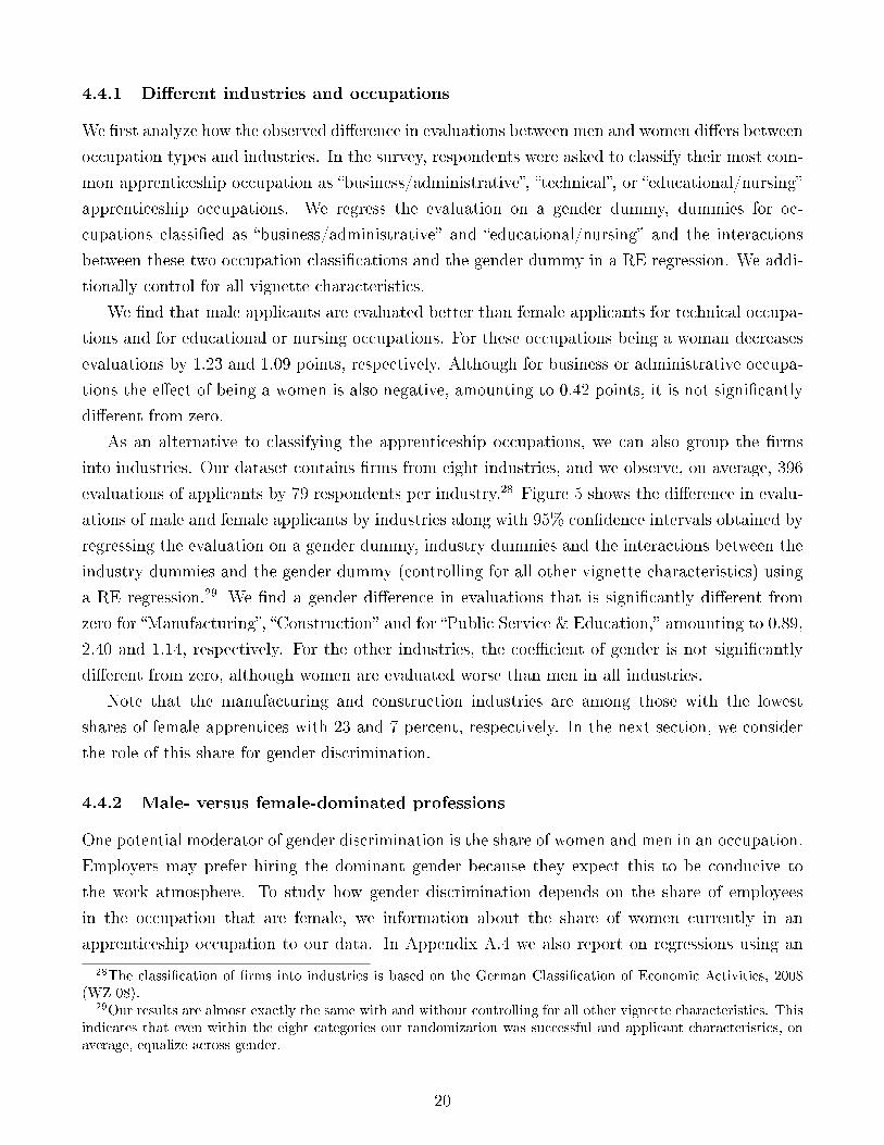
4.4.1 Di�erent industries and occupations
We �rst analyze how the observed di�erence in evaluations between men and women di�ers between
occupation types and industries. In the survey, respondents were asked to classify their most com-
mon apprenticeship occupation as �business/administrative�, �technical�, or �educational/nursing�
apprenticeship occupations. We regress the evaluation on a gender dummy, dummies for oc-
cupations classi�ed as �business/administrative� and �educational/nursing� and the interactions
between these two occupation classi�cations and the gender dummy in a RE regression. We addi-
tionally control for all vignette characteristics.
We �nd that male applicants are evaluated better than female applicants for technical occupa-
tions and for educational or nursing occupations. For these occupations being a woman decreases
evaluations by 1.23 and 1.09 points, respectively. Although for business or administrative occupa-
tions the e�ect of being a women is also negative, amounting to 0.42 points, it is not signi�cantly
di�erent from zero.
As an alternative to classifying the apprenticeship occupations, we can also group the �rms
into industries. Our dataset contains �rms from eight industries, and we observe, on average, 396
evaluations of applicants by 79 respondents per industry.28 Figure 5 shows the di�erence in evalu-
ations of male and female applicants by industries along with 95% con�dence intervals obtained by
regressing the evaluation on a gender dummy, industry dummies and the interactions between the
industry dummies and the gender dummy (controlling for all other vignette characteristics) using
a RE regression.29 We �nd a gender di�erence in evaluations that is signi�cantly di�erent from
zero for �Manufacturing�, �Construction� and for �Public Service & Education,� amounting to 0.89,
2.40 and 1.14, respectively. For the other industries, the coe�cient of gender is not signi�cantly
di�erent from zero, although women are evaluated worse than men in all industries.
Note that the manufacturing and construction industries are among those with the lowest
shares of female apprentices with 23 and 7 percent, respectively. In the next section, we consider
the role of this share for gender discrimination.
4.4.2 Male- versus female-dominated professions
One potential moderator of gender discrimination is the share of women and men in an occupation.
Employers may prefer hiring the dominant gender because they expect this to be conducive to
the work atmosphere. To study how gender discrimination depends on the share of employees
in the occupation that are female, we information about the share of women currently in an
apprenticeship occupation to our data. In Appendix A.4 we also report on regressions using an
28The classi�cation of �rms into industries is based on the German Classi�cation of Economic Activities, 2008(WZ 08).
29Our results are almost exactly the same with and without controlling for all other vignette characteristics. Thisindicates that even within the eight categories our randomization was successful and applicant characteristics, onaverage, equalize across gender.
20
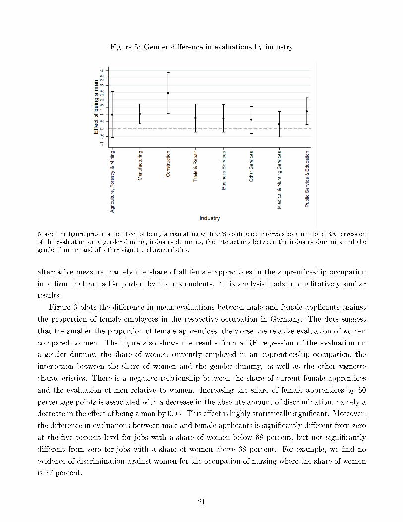
Figure 5: Gender di�erence in evaluations by industry
Note: The �gure presents the e�ect of being a man along with 95% con�dence intervals obtained by a RE regressionof the evaluation on a gender dummy, industry dummies, the interactions between the industry dummies and thegender dummy and all other vignette characteristics.
alternative measure, namely the share of all female apprentices in the apprenticeship occupation
in a �rm that are self-reported by the respondents. This analysis leads to qualitatively similar
results.
Figure 6 plots the di�erence in mean evaluations between male and female applicants against
the proportion of female employees in the respective occupation in Germany. The dots suggest
that the smaller the proportion of female apprentices, the worse the relative evaluation of women
compared to men. The �gure also shows the results from a RE regression of the evaluation on
a gender dummy, the share of women currently employed in an apprenticeship occupation, the
interaction between the share of women and the gender dummy, as well as the other vignette
characteristics. There is a negative relationship between the share of current female apprentices
and the evaluation of men relative to women. Increasing the share of female apprentices by 50
percentage points is associated with a decrease in the absolute amount of discrimination, namely a
decrease in the e�ect of being a man by 0.93. This e�ect is highly statistically signi�cant. Moreover,
the di�erence in evaluations between male and female applicants is signi�cantly di�erent from zero
at the �ve percent level for jobs with a share of women below 68 percent, but not signi�cantly
di�erent from zero for jobs with a share of women above 68 percent. For example, we �nd no
evidence of discrimination against women for the occupation of nursing where the share of women
is 77 percent.
21

Figure 6: Gender di�erence in evaluations by share of women
Note: The dots represent gender di�erences in the evaluation of applicants for apprenticeship occupations with agiven share of women. The solid line shows the e�ect of being a man obtained by a RE regression of the evaluation ona gender dummy, the share of women currently employed in an apprenticeship occupation, the interaction betweenthe share of women and the gender dummy and all other vignette characteristics. The dashed lines indicate 95%con�dence intervals for this e�ect.
Following the literature, we also split the occupations into three groups. We call those oc-
cupations with a national average of 0 to 33 percent female apprentices male-dominated, those
with a share of 33 to 66 percent gender balanced and those with a share of 67 to 100 percent
female apprentices female-dominated.30 We regress our evaluations on a gender dummy and both
the interaction terms of male-dominated jobs and gender as well as female-dominated jobs and
gender, that is, we interact both the indicator for female-dominated and for male-dominated jobs
with the gender dummy within one regression. For gender-balanced apprenticeship occupations,
we neither �nd signi�cant evidence of discrimination against men nor against women (see Table 3).
There is no signi�cant di�erence in discrimination between female-dominated and gender-neutral
occupations. Hence, we do not �nd evidence of discrimination against men in female-dominated
jobs in contrast to results in the literature. For male-dominated jobs, the e�ect of being a woman
is statistically signi�cantly di�erent from zero and amounts to -1.51 points. This is evidence of
discrimination against women in male-dominated jobs.
30The results are robust to using cut-o�s at 30 percent and 70 percent as in Weichselbaumer, 2004.
22

Table 3: Discrimination and gender ratio of occupations
Variable Coe�cient SE
Female -0.45 0.344
Female+Female*Female-dominated -0.37
Female+Female*Male-dominated -1.51**
Notes: The table displays the coe�cients and the standard errors
from a random e�ects regression of the evaluations on a gender
dummy, an indicator for female-dominated occupations, an indicator
for male-dominated occupations, interaction terms between the gen-
der dummy and the two occupation class indicators (�Female*Female-
dominated� and �Female*Male-dominated�), and other vignette char-
acteristics.
4.4.3 High- versus low-status occupations
The literature presents evidence that discrimination against women is more severe for occupations
associated with a high social status (for an overview, see Riach and Rich, 2002). We analyze how
gender discrimination varies with several variables related to occupational status. In particular,
we investigate the relationship between gender discrimination and the average salary, the typical
school-leaving quali�cation required for an apprenticeship, and two indices of occupational status.
Salaries
For the analysis of the salaries, we merge average hourly wages to our professions via the KldB
2010. The wages are national averages provided by the Federal Statistical O�ce (Destatis). We
end up with 117 di�erent hourly wages, ranging from 9.05 Euro per hour to 24.95 Euro per hour.
Our dataset also contains information on the average monthly wages of all workers in a �rm. Based
on these data, we construct two additional measures of salaries. The analyses using these data can
be found in Appendix A.5. The results are in line with the main results using hourly wage data
for the di�erent occupations presented in this section.
Figure 7 displays how the di�erence in evaluations between men and women varies with the
hourly wage. The graphical evidence suggests no clear linear relationship. The �gure also contains
the gender e�ect for di�erent wages obtained by regressing the evaluation on a gender dummy,
the average hourly wage of an occupation, their interactions, and the vignette characteristics. We
see that the negative e�ect of being a woman slightly decreases in absolute terms with higher
wages, and the e�ect of being a man is not signi�cantly di�erent from zero for very high wages.
Overall, there is no clear linear relationship between the amount of discrimination and the salary
of a profession.
To allow for a non-linear e�ect, we divide the wage distribution at the 0.33-quantile and the 0.66-
23
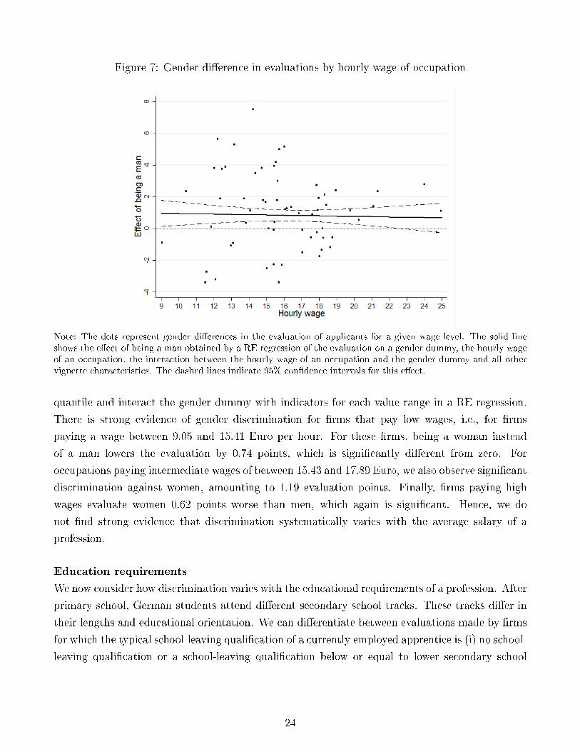
Figure 7: Gender di�erence in evaluations by hourly wage of occupation
Note: The dots represent gender di�erences in the evaluation of applicants for a given wage level. The solid lineshows the e�ect of being a man obtained by a RE regression of the evaluation on a gender dummy, the hourly wageof an occupation, the interaction between the hourly wage of an occupation and the gender dummy and all othervignette characteristics. The dashed lines indicate 95% con�dence intervals for this e�ect.
quantile and interact the gender dummy with indicators for each value range in a RE regression.
There is strong evidence of gender discrimination for �rms that pay low wages, i.e., for �rms
paying a wage between 9.05 and 15.41 Euro per hour. For these �rms, being a woman instead
of a man lowers the evaluation by 0.74 points, which is signi�cantly di�erent from zero. For
occupations paying intermediate wages of between 15.43 and 17.89 Euro, we also observe signi�cant
discrimination against women, amounting to 1.19 evaluation points. Finally, �rms paying high
wages evaluate women 0.62 points worse than men, which again is signi�cant. Hence, we do
not �nd strong evidence that discrimination systematically varies with the average salary of a
profession.
Education requirements
We now consider how discrimination varies with the educational requirements of a profession. After
primary school, German students attend di�erent secondary school tracks. These tracks di�er in
their lengths and educational orientation. We can di�erentiate between evaluations made by �rms
for which the typical school-leaving quali�cation of a currently employed apprentice is (i) no school-
leaving quali�cation or a school-leaving quali�cation below or equal to lower secondary school
24
(Hauptschule), (ii) intermediate secondary school (Realschule), or (iii) high school (Gymnasium).31
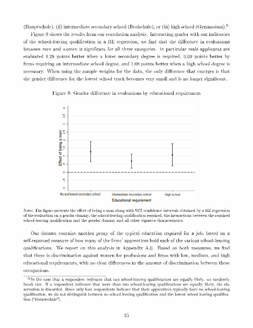
Figure 8 shows the results from our correlation analysis. Interacting gender with our indicators
of the school-leaving quali�cation in a RE regression, we �nd that the di�erence in evaluations
between men and women is signi�cant for all three categories. In particular male applicants are
evaluated 1.28 points better when a lower secondary degree is required, 0.69 points better by
�rms requiring an intermediate school degree, and 1.08 points better when a high school degree is
necessary. When using the sample weights for the data, the only di�erence that emerges is that
the gender di�erence for the lowest school track becomes very small and is no longer signi�cant.
Figure 8: Gender di�erence in evaluations by educational requirement
Note: The �gure presents the e�ect of being a man along with 95% con�dence intervals obtained by a RE regressionof the evaluation on a gender dummy, the school-leaving quali�cation required, the interactions between the requiredschool-leaving quali�cation and the gender dummy and all other vignette characteristics.
Our dataset contains another proxy of the typical education required for a job, based on a
self-reported measure of how many of the �rms' apprentices hold each of the various school-leaving
quali�cations. We report on this analysis in Appendix A.6. Based on both measures, we �nd
that there is discrimination against women for professions and �rms with low, medium, and high
educational requirements, with no clear di�erences in the amount of discrimination between these
occupations.
31In the case that a respondent indicates that two school-leaving quali�cations are equally likely, we randomlybreak ties. If a respondent indicates that more than two school-leaving quali�cations are equally likely, the ob-servation is discarded. Since only four respondents indicate that their apprentices typically have no school-leavingquali�cation, we do not distinguish between no school-leaving quali�cation and the lowest school-leaving quali�ca-tion (�Hauptschule�).
25

Occupational Status
Various measures of occupational status have been discussed in the literature (Ganzeboom and
Treiman, 2003). We employ the International Socio-Economic Index of occupational status (ISEI-
08) which is a socioeconomic measure of occupational status.32 It is based on the assumption
that occupational status determines how education is transformed into earnings.33 The index
was obtained using data from 2002 to 2007 on 200,000 individuals from more than 40 countries
(Ganzeboom, 2010). In our sample the ISEI is lowest for unskilled agricultural laborers who have
a score of 11.74 and highest for application programmers with a score of 74.66. The average score
is 36.92 and applies, for instance, to electrical mechanics.
Figure 9 displays the average di�erences in evaluations between male and female applicants for
di�erent values of the index of socioeconomic status. Male applicants are evaluated better than
female applicants for the majority of status scores. The �gure further suggests a negative relation-
ship between the di�erence in evaluations of male and female applicants and the socioeconomic
status of an occupation. This is in line with the result we obtain when we interact the socioeco-
nomic measure of occupational status with gender and run a RE estimation on a gender dummy,
the ISEI, the interaction between them as well as the vignette characteristics (see also Figure 9).
There is a sizable negative baseline e�ect of being female on the evaluations, while an increase in
the status of an occupation is associated with a decrease in gender discrimination as indicated by
a signi�cant coe�cient on the interaction term. In line with this, we �nd a statistically signi�cant
discrimination of 1.24 points for waitresses but no evidence of discrimination for application pro-
grammers (e�ect size=0.10). Using the weighting factor, the coe�cient on the interaction term
does not change in size, but fails to be statistically signi�cant at the 5 percent level.
We employ a second indicator of occupational status, the Standard International Occupation
Prestige Score (SIOPS) which is a measure of occupational prestige (Treiman, 1977). It is obtained
by asking individuals to assess the popularity of occupations.34 In our dataset, the scores of
occupational prestige range from 16, assigned to fast food sellers, to 60 for denturists. Similarly,
unskilled agricultural laborers and waiters score very low when it comes to occupational prestige
32The ISEI-08 is the International Socio-Economic Index of occupational status estimated for the ISCO-08,a classi�cation of occupations based on skill level and skill specialization. We rely on the conversion providedby Ganzeboom and Treiman (2017). Since in our dataset �rms are categorized according to the KldB 2010,we �rst add the ISCO-08 to our data, that is, we assign one unit group of the ISCO-08 (four-digit) to everyoccupational type of the KldB 2010 (�ve-digit). We do this by using the conversion key provided by the FederalEmployment Agency, see https://statistik.arbeitsagentur.de/Navigation/Statistik/Grundlagen/Klassi�kation-der-Berufe/KldB2010/Arbeitshilfen/Umsteigeschluessel/Umsteigeschluessel-Nav.html.
33The ISEI of an occupation is found by scaling occupational groups as a mediating variable such that thedirect e�ects of education on earnings are minimized and e�ects of education on earnings through occupation aremaximized. This leads to two coe�cients, one linking occupational status to education and one relating occupationalstatus to income that are used as weights to produce status scores based on the average level of education andearnings of an occupation.
34Individuals are asked to rate, for instance, the social prestige, the social standing, or the desirability of anoccupation. Treiman matched these prestige scores to occupations by using data from 60 countries. This measureof occupational prestige might capture additional dimensions of occupational status that are not captured by thesocioeconomic measure.
26
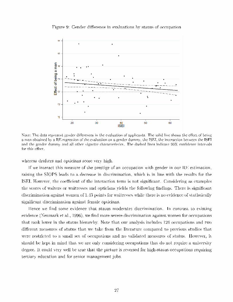
Figure 9: Gender di�erence in evaluations by status of occupation
Note: The dots represent gender di�erences in the evaluation of applicants. The solid line shows the e�ect of beinga man obtained by a RE regression of the evaluation on a gender dummy, the ISEI, the interaction between the ISEIand the gender dummy and all other vignette characteristics. The dashed lines indicate 95% con�dence intervalsfor this e�ect.
whereas drafters and opticians score very high.
If we interact this measure of the prestige of an occupation with gender in our RE estimation,
raising the SIOPS leads to a decrease in discrimination, which is in line with the results for the
ISEI. However, the coe�cient of the interaction term is not signi�cant. Considering as examples
the scores of waiters or waitresses and opticians yields the following �ndings. There is signi�cant
discrimination against women of 1.43 points for waitresses while there is no evidence of statistically
signi�cant discrimination against female opticians.
Hence we �nd some evidence that status moderates discrimination. In contrast to existing
evidence (Neumark et al., 1996), we �nd more severe discrimination against women for occupations
that rank lower in the status hierarchy. Note that our analysis includes 126 occupations and two
di�erent measures of status that we take from the literature compared to previous studies that
were restricted to a small set of occupations and no validated measures of status. However, it
should be kept in mind that we are only considering occupations that do not require a university
degree. It could very well be true that the picture is reversed for high-status occupations requiring
tertiary education and for senior management jobs.
27

4.4.4 Firm size, professionalization of the hiring procedure, and tightness of the
labor market
Previous research has found a negative relationship between �rm size and discrimination (Engels,
2015, Akar et al., 2014). If the size of the �rm is somehow re�ected in the individual evaluations
made by our respondents, we would expect discrimination to be a decreasing function of �rm size.
We measure the size of the �rm by the number of employees in the �rm and create four categories
of one to 19 employees, 20 to 99, 100 to 199 and 200 or more.35
Figure 10 shows that, controlling for the vignette characteristics, for applicants evaluated by
the smallest �rms (1 to 19 employees) the disadvantage of female applicants is the biggest and
amounts to 1.26 points. The disadvantage is smaller for the other three categories, but it is still
sizeable and statistically signi�cant, and no linear relationship between �rm size and the amount
of discrimination emerges.
Figure 10: Evaluation of �ctitious applicants by gender and �rm size
Note: The �gure presents the e�ect of being a man along with 95% con�dence intervals obtained by a RE regressionof the evaluation on a gender dummy, the �rm size measured by the number of employees, the interactions betweenthe �rm size and the gender dummy and all other vignette characteristics.
When we use the number of apprenticeships in the �rm instead of the number of employees
as a measure of �rm size, we again �nd no clear evidence that discrimination depends on �rm
size. The coe�cient on the interaction term between gender and the number of apprentices is not
signi�cantly di�erent from zero. The estimated e�ect of being female is -0.86 for �rms with four
apprentices (the median) and -0.77 for the 0.9-quantile (31 apprentices). In both cases, the gender
35We only count those employees for whom the �rm has to make social security payments.
28
e�ect is signi�cantly di�erent from zero. Only for �rms with a very large number of apprentices,
the gender e�ect does no longer reach statistical signi�cance.
A related variable potentially moderating gender discrimination is the professionalization of the
hiring procedure. A more professionalized and standardized recruitment process might counteract
gender discrimination, for example because standardized evaluation criteria are applied or because
managers with a taste for discrimination have to justify their decisions vis-à-vis others. Of course,
the evidence from our vignettes can only pick this up if individual managers who respond to our
survey have internalized the features of their �rms recruitment process. We measure a �rm's
degree of professionalization by the number of steps that a �rm's recruitment process typically
takes. These include, for example, the job interview, recruitment tests using work-related or
school-related questions, intelligence tests or personality tests, or trial work in the �rm. Clearly,
not all of the steps are required in every �rm, but we interpret a lack of many of these steps as
a lower level of professionalization. If we interact the number of steps in the recruitment process
linearly with gender, we �nd the coe�cient on the interaction term to be -0.09 and not signi�cantly
di�erent from zero. There is also no evidence that discrimination depends on the number of steps if
we use a dummy for more than three steps or a dummy for more than four steps in the recruitment
process.
Finally, we consider whether labor market conditions moderate gender discrimination. Speci�-
cally, human resource managers can be expected to discriminate less against women if they face a
limited supply of applicants. As an indicator of labor market tightness, we look at the percentage
of apprenticeships of an occupation in a �rm that have remained un�lled in the past years (a
categorical variable with the categories 0, 25% or less, 25 to 50%, and 50% or more). We �nd no
evidence of gender discrimination if more than 50 percent of the apprenticeships have remained
un�lled (e�ect size: -0.30), but signi�cantly more and statistically signi�cant discrimination if only
25 to 50 percent (e�ect size: -1.40), less than 25 percent (e�ect size: -1.38) or no apprenticeships
(e�ect size: -0.84) have remain un�lled in the last three years. Hence, for those �rms that have
trouble �lling their job openings, we �nd no indication of discrimination.
In summary, we �nd little evidence that the size of a �rm or the degree of professionalization
of the recruitment procedure have a systematic in�uence on discrimination at the early stage of
the selection process that we are focusing on. On the other hand, we observe that human resource
managers seem to discriminate less when the supply of suitable applicants is low.
4.5 Disentangling the e�ects of �rms, occupations, and industries
The previous sections were devoted to the analysis of how discrimination varies with several �rm-
related or occupation-related moderator variables. In this section we attempt to determine which
of these variables have explanatory power for the observed gender di�erence. Existing �eld exper-
iments have analyzed the e�ect of some of these moderators alone, but it is likely that by varying,
29

for example, the share of female employees in an occupation, these studies also vary other modera-
tor variables such as the status of these occupations, the salary etc. In fact, the share of currently
employed female apprentices and the variables related to status (educational requirements, salaries,
status indices) are weakly correlated in our sample.36
We consider the e�ects of all our variables of interest in one regression. Thus, we employ
interaction terms between the gender dummy and all moderator variables analyzed in the pre-
vious subsection. We then regress the applicant's evaluation on our moderator variables and
the interaction between these moderators and gender.37 We additionally control for all vignette
characteristics. For comparability, we standardize all variables such that the coe�cients can be
interpreted in terms of standard deviations.
In a �rst step, we include the variables related to status, namely the wage paid, the education
required, and one of the status measures in the RE regression.38 The results can be found in
columns (1) and (2) of Table 4. Column (1) shows that when using the ISEI, the coe�cients on
the interaction terms between the hourly wage and gender, the education index and gender, and the
ISEI and gender are all not statistically di�erent from zero. The same holds true for the interaction
terms between gender and �rm size as measured by the number of apprentices, between gender and
the number of steps in the recruitment process, between gender and labor market tightness, and
gender and the dummies for the classes of occupations (business or administrative and educational
or nursing). Hence, we �nd no evidence that any of these variables are moderating the gender
di�erence in evaluations.
In contrast, we �nd a positive e�ect for the interaction between the share of female apprentices
and gender. An increase in the share of currently employed female apprentices by one standard
deviation leads to a decrease in the e�ect of being female on the evaluation by 0.84 points. This
e�ect is highly signi�cant. It is also relatively large, since it is bigger in absolute terms than the
e�ect of having only an intermediate (3.4) instead of a relatively good GPA (2.8) on evaluations
(not reported in the table). Quantitatively, it implies that an increase in the share of female
apprentices by 50 percentage points raises female evaluations relative to male evaluations by 1.30
36In particular, the share of female apprentices is weakly positively correlated with the educational requirementsof an occupation (r=0.27 with the typical school-leaving degree and r=0.27 using the education index). It isweakly negatively correlated with the hourly wage of an apprenticeship occupation (r=-0.17). The share of femaleapprentices is moderately positively correlated with the ISEI (r=0.56) and weakly positively correlated with theSIOPS (r=0.39).
37The moderator variables are the occupation classi�cation of the apprenticeship as technical, busi-ness/administrative, or educational/nursing, share of women as apprentices in the �rm, average hourly wage ofan occupation, educational requirement of an occupation measured by the index, status index (ISEI or SIOPS),�rm size measured by the number of apprentices in the �rm, professionalization of the human resource managementand labor market tightness measured by the ratio of applicants invited to the next step of the recruitment processto applications received. The main results are unchanged if we use the number of employers as the measure of �rmsize, the Classi�cation of Economic Activities instead of the classi�cation of apprenticeship occupations into techni-cal, business/administrative, or educational/nursing occupations and education indicators instead of the educationindex.
38For ease of interpretation, we use the education index introduced in Appendix A.6 where a higher numberstands for more demanding educational requirements.
30
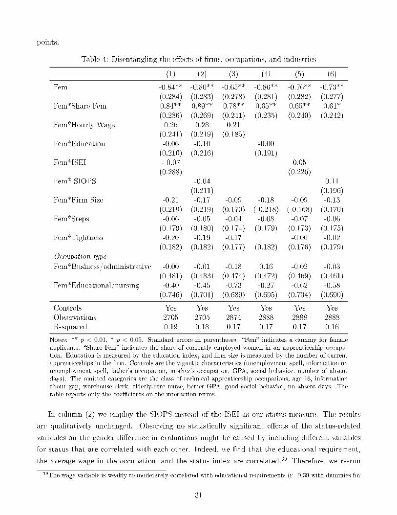
points.
Table 4: Disentangling the e�ects of �rms, occupations, and industries
(1) (2) (3) (4) (5) (6)
Fem -0.84** -0.80** -0.65** -0.86** -0.76** -0.73**(0.284) (0.283) (0.278) (0.281) (0.282) (0.277)
Fem*Share Fem 0.84** 0.89** 0.78** 0.65** 0.65** 0.61*(0.286) (0.269) (0.241) (0.235) (0.240) (0.242)
Fem*Hourly Wage 0.26 0.28 0.21(0.241) (0.219) (0.185)
Fem*Education -0.06 -0.10 -0.00(0.216) (0.216) (0.191)
Fem*ISEI - 0.07 0.05(0.288) (0.226)
Fem* SIOPS -0.04 0.11(0.211) (0.196)
Fem*Firm Size -0.21 -0.17 -0.09 -0.18 -0.09 -0.13(0.219) (0.219) (0.170) ( 0.218) ( 0.168) (0.170)
Fem*Steps -0.06 -0.05 -0.04 -0.08 -0.07 -0.06(0.179) (0.180) (0.174) (0.179) (0.173) (0.175)
Fem*Tightness -0.20 -0.19 -0.17 -0.06 -0.02(0.182) (0.182) (0.177) (0.182) (0.176) (0.179)
Occupation type
Fem*Business/administrative -0.00 -0.01 -0.18 0.16 -0.02 -0.03(0.481) (0.483) (0.474) (0.472) (0.469) (0.461)
Fem*Educational/nursing -0.40 -0.45 -0.73 -0.27 -0.62 -0.58(0.746) (0.701) (0.689) (0.695) (0.734) (0.690)
Controls Yes Yes Yes Yes Yes YesObservations 2705 2705 2874 2888 2888 2888R-squared 0.19 0.18 0.17 0.17 0.17 0.16
Notes: ** p < 0.01, * p < 0.05. Standard errors in parentheses. �Fem� indicates a dummy for femaleapplicants. �Share Fem� indicates the share of currently employed women in an apprenticeship occupa-tion. Education is measured by the education index, and �rm size is measured by the number of currentapprenticeships in the �rm. Controls are the vignette characteristics (unemployment spell, information onunemployment spell, father's occupation, mother's occupation, GPA, social behavior, number of absentdays). The omitted categories are the class of technical apprenticeship occupations, age 16, informationabout gap, warehouse clerk, elderly-care nurse, better GPA, good social behavior, no absent days. Thetable reports only the coe�cients on the interaction terms.
In column (2) we employ the SIOPS instead of the ISEI as our status measure. The results
are qualitatively unchanged. Observing no statistically signi�cant e�ects of the status-related
variables on the gender di�erence in evaluations might be caused by including di�erent variables
for status that are correlated with each other. Indeed, we �nd that the educational requirement,
the average wage in the occupation, and the status index are correlated.39 Therefore, we re-run
39The wage variable is weakly to moderately correlated with educational requirements (r=0.39 with dummies for
31

our RE estimation including only one of the status-related variables at a time (see columns (3)
to (6)). We again �nd no evidence that any of the status-related variables (salary, educational
requirement, ISEI or SIOPS) explain the gender di�erences in evaluations. A detailed discussion
of these results can be found in Appendix A.7.
We draw a number of conclusions from the analysis presented in this section. The di�erence
in evaluations between male and female applicants is mainly explained by the share of female
applicants in an occupation. Discrimination against female applicants is a negative function of the
share of female apprentices currently employed. Further analyses based on a sample split for male
and female applicants show that most of the di�erence is due to women being evaluated better when
the share of female applicants increases while the di�erence is not caused by a worse evaluation
of male applicants when the share of women increases.40 We �nd no evidence that the variables
related to status, such as the average hourly wage of an occupation, an occupation's educational
requirements, and indices of occupational status, as well as �rm size, the type of the occupation,
or the professionalization of the recruitment process can explain a signi�cant proportion of the
observed gender di�erence.
5 Conclusion
We document that female job applicants are evaluated worse than male applicants by respondents
from a large sample of German �rms. No matter how we split our sample by observable charac-
teristics of �rms, of occupations, or of the job applicants, discrimination against women is almost
always observed, albeit to a varying degree. Our �ndings cannot be explained by di�erences in the
expected variance of the unobserved productivity of men and women. The observed gender di�er-
ences are also unlikely to represent statistical discrimination caused by the productivity signals of
the underrepresented gender being less reliable.
Gender discrimination di�ers between industries, with the construction industry, manufacturing
and the education and public service sector displaying a signi�cant penalty for female applicants.
Also, women fare signi�cantly worse than men both in male-dominated professions and in occu-
pations requiring only a lower secondary school degree. There is no clear relationship between
the salaries of professions and gender discrimination, but we �nd that with the increasing social
status of an occupation (as measured by the two indices ISEI and SIOPS), the evaluations of
women relative to men improve. This is also true for very tight labor markets. Finally, there is no
correlation between the size of the �rm and the structure of the recruitment procedure with the
amount of gender discrimination.
education levels, r=0.40 with the education index) and weakly correlated with both measures of occupational status(r=0.39 with ISEI, r=0.25 with SIOPS). The correlation between educational requirements and the status indexesis weakly to moderately positive (r=0.31 (r=0.32) using indicators for education levels (the education index) andthe SIOPS, r=0.42 (r=0.43) using indicators for education (the education index) and the ISEI).
40The regressions are not reported in the paper, but are available upon request from the authors.
32

When we consider the relationship between gender discrimination and all �rm- and occupation-
speci�c moderator variables simultaneously, only the gender ratio in a profession shows a signi�cant
e�ect on how much a �rm's evaluation of an applicant depends on the gender. In particular, women
su�er large penalties in male-dominated professions.
Regarding the method of factorial survey design, the responses that we have collected lead to
surprisingly clear di�erences between the evaluations of our candidates, with the main variables
such as grades and age, having the expected e�ects. We believe that the validity of the answers we
received is due to the fact that our survey was conducted as part of a regular panel, and that we
presented human resource managers with vignettes structured like a CV where such evaluations
of CVs are part of the respondents' everyday work.
One unobserved variable that could determine the productivity in certain professions is physical
strength. If employers expect men to be, on average, stronger than women, this could give them
an advantage, for example, in the construction industry or in manufacturing where we �nd the
largest di�erences in evaluations. We would like to make two comments regarding this concern.
First, many of the most common professions with a strong male dominance do not require physical
strength, such as a mechatronics engineer, and many similar technical occupations. Second, the
amount of strength needed for certain tasks is a function of the tools developed for them. �Handle
size and tool weight are designed to accommodate the size and strength of men,� as stated in a
report to OSHA (Occupational Safety and Health Administration) of the US Department of Labor
(1999), which recommends changes necessary to allow women to enter the construction industry.
While we cannot exclude that di�erences in physical strength can explain some of the di�erences in
the evaluations of men and women, this would mean, however, that at least part of the productivity
di�erential can be removed by appropriate adjustments of the workplace.
Our results clearly indicate that in male-dominated professions, employers are less likely to hire
women compared to men. Thus, discrimination is likely to push women into female-dominated
jobs. This can perpetuate gender imbalances and contribute to a shortage of labor supply, for
example, in technical professions, especially if women anticipate the �rms' responses and therefore
apply at a lower rate to professions in which they are underrepresented. Given the design of our
study, we can only make causal statements regarding the e�ect of gender on the evaluation of
an applicant and not regarding the e�ect of the gender ratio on discrimination. However, our
results are consistent with policies that aim at a su�cient number of women in jobs where they
are underrepresented to remove the existing obstacles for women and reach a tipping point. Such
policies could change the gender stereotypes attached to these jobs and the atmosphere at the
workplace that are often seen as culprits of the self-perpetuating gender di�erentials.
33

References
[1] Advisory Committee on Construction Safety and Health (1999). Women in the Construction
Workplace: Providing Equitable Safety and Health Protection. Submitted to the Occupa-
tional Safety and Health Administration (OSHA), Department of Labor, USA. Retrieved
from https:// www.osha.gov/doc/accsh/haswicformal.html#ergonomics.
[2] Aigner, Dennis J., and Glen G. Cain (1977). Statistical theories of discrimination in labor
markets. ILR Review 30.2 : 175�187.
[3] Akar, G., B. Balkan, and S. Tumen (2014). Overview of Firm-Size and Gender Pay Gaps in
Turkey: The Role of Informal Employment.
[4] Altonji, J.G. and R.M. Blank (1999). Race and Gender in the Labor Market. In: Ashenfelter,
O. and D. Card (eds.). Handbook of Labor Economics. Vol. 3, chapter 48.
[5] Authoring Group Educational Reporting (2012). Education in Germany 2012. Bielefeld: W.
Bertelsmann Verlag.
[6] Azmat, and B. Petrongolo (2014). Gender and the Labor Market: What Have We Learned
From Field and Lab Experiments? Labour Economics 30, 32-40.
[7] Baethge, M., H. Solga and M. Wieck (2007). Berufsbildung im Umbruch - Signale eines
überfälligen Aufbruchs. Netzwerk Bildung. Berlin: Friedrich-Ebert-Stiftung.
[8] Bayard, K., Hellerstein, J., Neumark, D. and Troske, K. (2003). New evidence on sex segre-
gation and sex di�erences in wages from matched employee-employer data. Journal of labor
Economics, 21(4), 887�922.
[9] Bertrand, M. and S. Mullainathan (2004). Are Emily and Gregg More Employable Than Lak-
isha and Jamal? A Field Experiment on Labor Market Discrimination. American Economic
Review 94(4), 991�1013.
[10] BIBB [Bundesinstitut für Berufsbildung] (2012). Datenreport zum Berufsbildungsbericht
2012, Table A.4.10.2-5. Bonn: BIBB. Online: http://datenreport.bibb.de/html/4724.htm,
last access: 23.01.2015.
[11] BMBF [Bundesministerium für Bildung und Forschung] (2012). Bundesbericht Forschung und
Innovation 2012, Figure 2.3.37. Online: http://www.datenportal.bmbf.de/portal/2.3.37, last
access: 23.01.2015.
[12] Bohnet, I., A. van Geen, and M. Bazerman (2016). When Performance Trumps Gender Bias:
Joint Versus Separate Evaluation. Management Science 62(5), 1225�1234.
34
[13] Booth, A. and A. Leigh (2010). Do employers discriminate by gender? A �eld experiment in
female-dominated occupations. Economic Letters 107, 236�238.
[14] Cohen, S. L., and K.A. Bunker (1975). Subtle e�ects of sex role stereotypes on recruiters'
hiring decisions. Journal of Applied Psychology, 60, 566�572.
[15] Dustmann, C. (2004). Parental background, secondary school track choice, and wages. Oxford
Economic Papers 56.2: 209-230.
[16] Engels, S.I. (2015). The E�ect of Firm Size on Gender Wage Discrimination in the Netherlands.
Economics. Retrieved from http://hdl.handle.net/2105/30064.
[17] Fershtman, C. and U. Gneezy (2001). Discrimination in a Segmented Society: An Experimen-
tal Approach, Quarterly Journal of Economics 116, 351�377.
[18] Firth, Michael (1982). Sex discrimination in job opportunities for women. Sex Roles, 8 (8),
891�901.
[19] Fitzenberger, B., S. Licklederer, and M. Zimmermann (2015). Übergänge von der allgemein-
bildenden Schule in beru�iche Ausbildung und Arbeitsmarkt: Die ökonomische Perspektive.
Forthcoming in: Seifried, J., Seeber, S. und Ziegler, B. (Ed.): Jahrbuch der berufs- und
wirtschaftspä dagogischen Forschung 2015. Schriftenreihe der Sektion Berufs-und Wirtschaft-
spädagogik. Opladen: Barbara Budrich.
[20] Ganzeboom, H.B.G. (2010). A New International Socio-Economic Index [ISEI] of Occupa-
tional Status for the International Standard Classi�cation of Occupation 2008 [ISCO-08]
Constructed with Data from the ISSP 2002-2007; with an Analysis of Quality of Occupa-
tional Measurement in ISSP. Paper presented at Annual Conference of International Social
Survey Programme, Lisbon, May 1 2010.
[21] Ganzeboom, H.B.G. and D.J. Treiman (2017). International Strati�cation and Mobil-
ity File: Conversion Tools. Amsterdam: Department of Social Research Methodology,
http://www.harryganzeboom.nl/ismf/index.htm. Last revision on April 7, 2017.
[22] Ganzeboom, H.B.G. and D.J. Treiman (2003). Three Internationally Standardised Measures
for Comparative Research on Occupational Status. Pages 159-193. In: Jürgen H.P. Ho�meyer-
Zlotnik & Christof Wolf (Eds.), Advances in Cross-National Comparison. A EuropeanWorking
Book for Demographic and Socio-Economic Variables. New York: Kluwer Academic Press.
[23] Gerhards, C., S. Mohr and K. Troltsch (2016). BIBB Training Panel - An Establishment Panel
on Training and Competence Development 2014. gwa_1.0; Research Data Center at BIBB;
Bonn: Federal Institute for Vocational Education and Training. doi:10.7803/371.14.1.2.10.
35

[24] Heckman, J.J (1998). Detecting discrimination. The Journal of Economic Perspectives 12.2:
101�116.
[25] Heckman, J.J. and P. Siegelman (1993). The Urban Institute Audit Studies: Their Methods
and Findings.
[26] Jonsson, J.O., D.B. Grusky, M. Di Carlo, Pollak, R., and M. Brinton (2009). Microclass
Mobility. Social Reproduction in Four Countries. American Journal of Sociology 114 (4),
977�1036.
[27] Kaas, L. and C. Manger (2011). Ethnic Discrimination in Germany's Labor Market. German
Economic Review 13, 1�20.
[28] Knoll, B., N. Riedel, and E. Schlenker (forthcoming). He's A Chip O� The Old Block: The
Persistency of Occupational Choices Among Generations. LABOUR: Review of Labour Eco-
nomics and Industrial Relations.
[29] Kleven, H. J., C. Landais, and J.E. Sogaard (2017). Children and gender inequality: Evidence
from Denmark. Unpublished manuscript, London School Econ.
[30] Levinson, R.M. (1975). Sex Discrimination And Employment Practices: An Experiment With
Unconventional Job Inquiries. Social Problems 22, 533�543.
[31] List, J. (2004). The Nature and Extent of Discrimination in the Market Place: Evidence from
the Field. Quarterly Journal of Economics 119, 49�90.
[32] Muchinsky, P. M. and Harris, S. L. (1977). The e�ect of applicant sex and scholastic standing
on the evaluation of job applicant resumes in sex-typed occupations. Journal of Vocational
Behavior, 11(1), 95�108.
[33] Neumark, D., R.J. Bank and K.D. Van Nort (1996). Sex Discrimination in Hiring in the
Restaurant Industry: An Audit Study. Quarterly Journal of Economics 111(3), 915�42.
[34] Neumark, D. (2012). Detecting Discrimination in Audit and Correspondence Studies. Journal
of Human Resources 47(4), 1128�1157.
[35] Olian, J.D., D.P. Schwab and Y. Haberfeld (1988). The impact of applicant gender com-
pared to quali�cations on hiring recommendations: A meta-analysis of experimental studies.
Organizational Behavior and Human Decision Processes, 41(2), 180�195.
[36] Petit, P. (2007). The E�ects Of Age And Family Constraints On Gender Hiring Discrimina-
tion: A Field Experiment In The French Financial Sector. Labour Economics 14, 371�391.
36

[37] Riach, P. A. and Rich, J. (1987). Testing For Sexual Discrimination in the Labor Market.
Australian Economic Papers 26, 165�178.
[38] Riach, P. A. and Rich, J. (2002). Field Experiments Of Discrimination In The Market Place.
Economic Journal 112, F480�F518.
[39] Riach, P. A. and Rich, J. (2006). An Experimental Investigation of Sexual Discrimination in
Hiring in the English Labor Market. Advances in Economic Analysis & Policy 6(2), article 1.
[40] Schein, Virginia E. (1973). The relationship between sex role stereotypes and requisite man-
agement characteristics. Journal of Applied Psychology 57(2), 95-100.
[41] Statistisches Bundesamt (Destatis) (2016). Verdienststrukturerhebung 2014 Fachserie 16 Heft
1.
[42] Treiman, D.J. (1977). Occupational Prestige in Comparative Perspective. New York: Aca-
demic Press.
[43] Weichselbaumer, D. (2004). Is it Sex or Personality? The Impact of Sex-Stereotypes on
Discrimination in Applicant Selection. Eastern Economic Journal 30, 159�86.
37

A Appendix
A.1 Introductory text for the vignette in English and the original Ger-
man vignette
�We will now show you short descriptions of �ve �ctitious persons. Please imagine that these
persons are applying for an apprenticeship for the most frequent apprenticeship occupation at your
company, either online or with a written application. All applications contain a good cover letter.
All applicants are from Germany. Please evaluate how likely it is that an applicant will receive an
invitation for the next step of the recruitment procedure in your company (after processing the
written application) based on the information provided in the CV.�
Figure 11: Example of a vignette as shown to the respondents
38

A.2 Detailed regression results
Table 5: Marginal e�ects of ordered probit estima-
tion
Evaluation Marginal e�ect Standard error
1 0.065** 0.013
2 0.024** 0.005
3 0.023** 0.004
4 0.014** 0.003
5 0.008** 0.002
6 -0.002* 0.001
7 -0.012** 0.003
8 -0.029** 0.006
9 -0.025** 0.005
10 -0.067** 0.013
Observations 3164
Notes: ** p < 0.01, * p < 0.05. The second column reports
the marginal e�ects of being female on the probability of
observing an evaluation as indicated by the �rst column.
The marginal e�ects are obtained from an ordered probit
estimation from the evaluation on the vignette characteris-
tics (see Table 2). Standard errors are obtained using the
Delta-method.
39
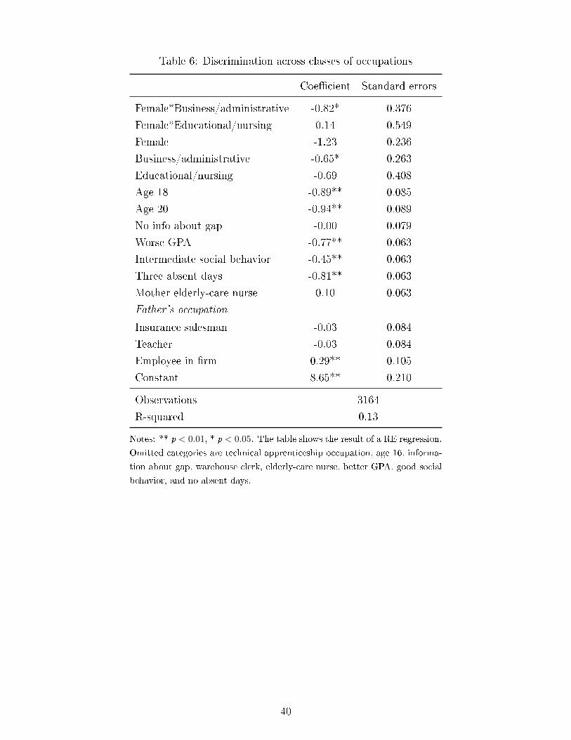
Table 6: Discrimination across classes of occupations
Coe�cient Standard errors
Female*Business/administrative -0.82* 0.376
Female*Educational/nursing 0.14 0.549
Female -1.23 0.236
Business/administrative -0.65* 0.263
Educational/nursing -0.69 0.408
Age 18 -0.89** 0.085
Age 20 -0.94** 0.089
No info about gap -0.00 0.079
Worse GPA -0.77** 0.063
Intermediate social behavior -0.45** 0.063
Three absent days -0.81** 0.063
Mother elderly-care nurse 0.10 0.063
Father's occupation
Insurance salesman -0.03 0.084
Teacher -0.03 0.084
Employee in �rm 0.29** 0.105
Constant 8.65** 0.210
Observations 3164
R-squared 0.13
Notes: ** p < 0.01, * p < 0.05. The table shows the result of a RE regression.
Omitted categories are technical apprenticeship occupation, age 16, informa-
tion about gap, warehouse clerk, elderly-care nurse, better GPA, good social
behavior, and no absent days.
40

Table 7: Discrimination across classes of �rms
Coe�cient Standard errors
Female*Agriculture, Forestry & Mining -0.66 0.925
Female*Manufacturing -0.70 0.571
Female*Construction -2.14* 0.841
Female*Trade & Repair -0.41 0.668
Female*Business Services -0.39 0.664
Female*Other Services -0.29 0.653
Female*Public Service & Education -0.89 0.649
Female -0.34 0.449
Agriculture, Forestry & Mining 0.29 0.682
Manufacturing -0.03 0.413
Construction -0.61 0.592
Trade & Repair -0.51 0.484
Business Services -0.76 0.473
Other Services -0.16 0.446
Public Service & Education -0.58 0.451
Age 18 -0.89** 0.085
Age 20 -0.93** 0.089
No info about gap -0.01 0.079
Worse GPA -0.77** 0.063
Intermediate social behavior -0.45** 0.063
Three absent days -0.81** 0.063
Mother elderly-care nurse 0.10 0.063
Father's occupation
Insurance salesman -0.02 0.084
Teacher -0.04 0.084
Employee in �rm 0.29** 0.105
Constant 8.78** 0.347
Observations 3164
R-squared 0.13
Notes: ** p < 0.01, * p < 0.05. The table shows the result of a RE regression.
Omitted categories are Medical & Nursing Services, age 16, information about gap,
warehouse clerk, elderly-care nurse, better GPA, good social behavior, and no absent
days. Classi�cation of �rms based on WZ 08.
41

Table 8: Discrimination and variables of interest
Variable of interest Share Female Wage Education ISEI SIOPS Firm Size Steps
Female*Variable of interest 1.85** 0.02 0.40 0.03* 0.03 0.00 -0.09
(0.539) ( 0.051) (0.289) (0.014) (0.023) (0.005) (0.138)
Female -1.66** -1.13 -1.70** -1.92** -2.28* -0.87** -0.57
(0.297) (0.861) (0.590) (0.558) (0.987) (0.185) (0.536)
Variable of interest -0.33 -0.10** -0.88** -0.02* -0.03 0.01** -0.12
(0.374) (0.036) (0.213) (0.010) (0.017) (0.003) (0.094)
Age 18 -0.88** -0.88** -0.91** -0.88** -0.88** -0.89** -0.89**
(0.086) (0.086) (0.088) (0.086) (0.086) (0.085) (0.085)
Age 20 -0.92** -0.93** -0.99** -0.92** -0.92** -0.94** -0.94**
(0.090) (0.090) (0.092) (0.090) (0.090) (0.089) (0.089)
No info about gap -0.01 -0.01 0.01 -0.01 -0.01 0.00 -0.01
(0.079) (0.079) ( 0.082) (0.079) (0.079) (0.079) (0.079)
Worse GPA -0.77** -0.77** -0.76** -0.77** -0.77** -0.77** -0.76**
(0.064) (0.064) (0.065) (0.063) (0.063) (0.063) (0.063)
Intermediate social behavior -0.47** -0.47** -0.47** -0.47** -0.47** -0.45** -0.45**
(0.064) (0.064) (0.065) (0.063) (0.063) (0.063) (0.063)
Three absent days -0.82** -0.82** -0.81** -0.82** -0.82** -0.81** -0.81**
(0.064) (0.064) (0.065) (0.063) (0.063) (0.063) (0.063)
Mother elderly-care nurse 0.11 0.12 0.11 0.12 0.12 0.11 0.10
(0.064) (0.064) (0.065) (0.063) (0.063) (0.063) (0.063)
Father's occupation
Insurance salesman -0.03 -0.04 -0.01 -0.03 -0.03 -0.02 -0.02
(0.085) (0.085) (0.087) (0.084) (0.084) (0.084) (0.084)
Teacher -0.05 -0.05 -0.05 -0.05 -0.05 -0.03 -0.03
(0.085) (0.085) (0.087) (0.085) (0.085) (0.084) (0.084)
Employee in �rm 0.29** 0.29** 0.36** 0.28** 0.28** 0.30** 0.29**
(0.106) (0.106) (0.109) (0.106) (0.106) (0.105) (0.105)
Constant 8.64** 10.19** 10.17** 9.39** 9.65** 8.34** 8.92**
( 0.248) (0.267) (0.456) (0.425) (0.712) (0.182) (0.391)
Observations 3106 3107 2938 3121 3121 3164 3164
R-squared 0.11 0.11 0.13 0.10 0.10 0.11 0.10
Notes: ** p < 0.01, * p < 0.05. The table shows the results of RE regressions. Education refers to the education
index and �rm size to the number of apprentices in a �rm. Omitted categories are age 16, information about gap,
warehouse clerk, elderly-care nurse, better GPA, good social behavior, and no absent days.
42

Table 9: Discrimination and required education
Coe�cient Standard Error
Female*intermediate secondary school 0.59 0.370
Female* high school 0.19 0.466
Female �1.28** 0.321
Intermediate secondary school -0.30 0.259
High school -0.86* 0.340
Age 18 -0.90** 0.088
Age 20 -0.98** 0.093
No info about gap 0.01 0.082
Worse GPA -0.76** 0.066
Intermediate social behavior -0.47** 0.066
Three absent days -0.82** 0.066
Mother elderly-care nurse 0.11 0.066
Father's occupation
Insurance salesman -0.02 0.087
Teacher -0.04 0.087
Employee in �rm 0.35** 0.109
Constant 8.82** 0.267
Observations 2923
R-squared 0.13
Notes: ** p < 0.01, * p < 0.05. The table shows the result of a RE regression.
Omitted categories are no or lowest secondary school required, age 16, information
about gap, warehouse clerk, elderly-care nurse, better GPA, good social behavior,
and no absent days.
43

Table 10: Discrimination and �rm size measured by the num-
ber of employees
Coe�cient Standard Error
Female* Size 2 0.57 0.484
Female* Size 3 0.24 0.592
Female* Size 4 0.46 0.474
Female -1.26** 0.365
Size 2 0.11 0.341
Size 3 -0.18* 0.421
Size 4 -0.02 0.331
Age 18 -0.89** 0.085
Age 20 -0.93** 0.089
No info about gap -0.01 0.079
Worse GPA -0.77** 0.063
Intermediate social behavior -0.45** 0.063
Three absent days -0.81** 0.063
Mother elderly-care nurse 0.11 0.063
Father's occupation
Insurance salesman -0.02 0.084
Teacher -0.02 0.084
Employee in �rm 0.29** 0.105
Constant 8.49** 0.284
Observations 3164
R-squared 0.10
Notes: ** p < 0.01, * p < 0.05. The table shows the result of a RE
regression. Firm size 2 is 20 to 99, �rm size 3 is 100 to 199, �rm size 4
is 200 or more employees. Omitted categories are 1 to 19 employees, age
16, information about gap, warehouse clerk, elderly-care nurse, better
GPA, good social behavior, and no absent days.
44

Table 11: Discrimination and professionalization of the recruitment process
Few steps: Steps ≤ 3 Few steps: Steps ≤ 4
Coe�cient Standard Error Coe�cient Standard Error
Female*Few steps 0.21 0.349 0.04 0.349
Female -1.01** 0.258 -0.93* 0.260
Few steps 0.19 0.247 0.42 0.247
Age 18 -0.89** 0.085 -0.89** 0.085
Age 20 -0.93** 0.089 -0.93** 0.089
No info about gap -0.01 0.079 -0.01 0.079
Worse GPA -0.77** 0.063 -0.77** 0.063
Intermediate social behavior -0.45** 0.063 -0.45** 0.063
Three absent days -0.81** 0.063 -0.81** 0.063
Mother elderly-care nurse 0.10 0.063 0.10 0.063
Father's occupation
Insurance salesman -0.02 0.084 -0.02 0.084
Teacher -0.03 0.084 -0.03 0.084
Employee in �rm 0.29** 0.105 0.29** 0.105
Constant 8.82** 0.224 8.15** 0.224
Observations 3164 3164
R-squared 0.10 0.10
Notes: ** p < 0.01, * p < 0.05. The table shows the results of RE regressions. �Few steps� is an indicator
for �rms with less than or exactly three [four] steps in their recruitment process in column 2 and 3 [4 and 5].
Omitted categories are more than three [four] steps in column 2 and 3 [4 and 5], age 16, information about
gap, warehouse clerk, elderly-care nurse, better GPA, good social behavior, and no absent days.
45
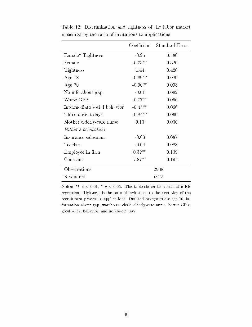
Table 12: Discrimination and tightness of the labor market
measured by the ratio of invitations to applications
Coe�cient Standard Error
Female* Tightness -0.25 0.580
Female -0.73** 0.320
Tightness 1.44 0.420
Age 18 -0.89** 0.089
Age 20 -0.96** 0.093
No info about gap -0.01 0.082
Worse GPA -0.77** 0.066
Intermediate social behavior -0.45** 0.066
Three absent days -0.84** 0.066
Mother elderly-care nurse 0.10 0.066
Father's occupation
Insurance salesman -0.03 0.087
Teacher -0.04 0.088
Employee in �rm 0.32** 0.109
Constant 7.87** 0.194
Observations 2938
R-squared 0.12
Notes: ** p < 0.01, * p < 0.05. The table shows the result of a RE
regression. Tightness is the ratio of invitations to the next step of the
recruitment process to applications. Omitted categories are age 16, in-
formation about gap, warehouse clerk, elderly-care nurse, better GPA,
good social behavior, and no absent days.
46

Table 13: Discrimination and tightness of the labor market mea-
sured by the number of un�lled apprenticeship positions
Coe�cient Standard Error
Female* vacancies <25% -0.54 0.524
Female* vacancies 25% to 50% -0.56 0.736
Female* vacancies >50% 0.55 0.729
Female -0.84** 0.202
vacancies <25% 0.21 0.346
vacancies 25 to 50% 0.92 0.535
vacancies >50% 0.74 0.444
Age 18 -0.90** 0.086
Age 20 -0.96** 0.090
No info about gap -0.00 0.079
Worse GPA -0.76** 0.064
Intermediate social behavior -0.45** 0.064
Three absent days -0.80** 0.064
Mother elderly-care nurse 0.10 0.064
Father's occupation
Insurance salesman -0.01 0.084
Teacher -0.04 0.085
Employee in �rm 0.32** 0.106
Constant 8.34** 0.194
Observations 3124
R-squared 0.11
Notes: ** p < 0.01, * p < 0.05. The table shows the result of a RE regres-
sion. Omitted categories are no vacancies in the apprenticeship occupation,
age 16, information about gap, warehouse clerk, elderly-care nurse, better
GPA, good social behavior, and no absent days.
47

A.3 External data sources
Table 14: External data sources
Variable Description of Data Source Key
Share of female apprentices Datenbank Auszubildende, Federal Institute for Vocational Education and KldB 2010
(main text) Training (BIBB) (for apprenticeship occupations regulated by the BBiG or HwO);
Beru�iche Schulen 2014 Fachserie 11 Reihe 2, Federal Statistics O�ce (Destatis)
(for other apprenticeship occupations)
Average hourly wage Verdienststrukturerhebung 2014 Fachserie 16 Heft 1, Federal Statistical O�ce KldB 2010
(main text) (Destatis)
International Socio-Economic Index International Strati�cation and Mobility File: Conversion Tools by Ganzeboom ISCO-08
of occupational status and Treiman
Standard International Occupation International Strati�cation and Mobility File: Conversion Tools by Ganzeboom ISCO-08
Prestige Score (SIOPS) and Treiman
Note: The table lists all datasets used that are not part of the Company Panel on Quali�cation and Competence Development of the BIBB
(Federal Institute of Vocational Education and Training).
A.4 Male- versus female-dominated professions using self-reported data
of the gender ratio of apprenticeships
Using the �rms' self-reported shares of currently employed female apprentices, the relationship
between this share and gender discrimination does not seem to be as clear-cut as for the national
averages of the share of female apprentices in a profession (see Figure 12). If we regress the
evaluation on a gender dummy, the share of female apprentices, the interaction term between
these two variables and other vignette characteristics, the coe�cient on the interaction term is
signi�cantly di�erent from zero and amounts to 1.54 (see also Figure 12). Thus, an increase by 50
percentage points is associated with an increase in the evaluation of female applicants relative to
male applicants by 0.77 points.
If we interact both the indicator for female-dominated and for male-dominated jobs with the
gender dummy in one regression, the results are as follows. For gender-balanced apprenticeships
we �nd neither evidence of discrimination against men nor against women. We again see a siz-
able negative e�ect of being female in male-dominated occupations (compared to gender-neutral
occupations). We �nd no signi�cant di�erence in discrimination between female-dominated and
gender-neutral occupations.
We take away two messages from this analysis using the self-reported shares of female appren-
tices in each �rm. First, the relationship between the self-reported share of female apprentices
and gender discrimination is less clear-cut than when we use national averages. Second, our main
�ndings about the in�uence of the share of female apprentices still hold.
48

Figure 12: Di�erence in evaluations between male and female applicants by share of women inapprenticeships per �rm
Note: The dots represent gender di�erences in the evaluation of applicants. The solid line shows the e�ect of beinga man obtained by a RE regression of the evaluation on a gender dummy, the self-reported share of women currentlyemployed in an apprenticeship occupation, the interaction between the share of women and the gender dummy andall other vignette characteristics. The dashed lines indicate 95% con�dence intervals for this e�ect.
A.5 High- versus low-wage occupations using self-reported wage data
The dataset contains information on the average monthly wages for workers in a �rm. Based
on this we construct two measures of (occupational) wages in order to relate the wage level to
discrimination. Note that respondents report monthly wages for all occupations in the �rm and
do not report the speci�c wages for the apprenticeship occupation we analyze. They report wages
separately for unskilled (�einfache Tätigkeit�), skilled (�quali�zierte Tätigkeit�), and highly-skilled
work (�hochquali�zierte Tätigkeit�). As our �rst measure we use the wages reported for employees
with skilled jobs (�quali�zierte Tätigkeit�), since these are typically the jobs performed by em-
ployees who have completed an apprenticeship. We use the midpoints of each of the three wage
categories for the respondents for which we only observe the categorized monthly wage. Monthly
wages then range from 1,050 Euro to 5,700 Euro. The mean monthly wage is 2,516 Euro.
Figure 13 displays how the di�erence in evaluations between men and women varies with the
monthly wage. The graphical evidence suggests that there might a negative relationship between
the di�erence in evaluations between male and female applicants and wage payments. In our
typical RE estimation, however, the coe�cient on the interaction term is not signi�cantly di�erent
from zero.
49
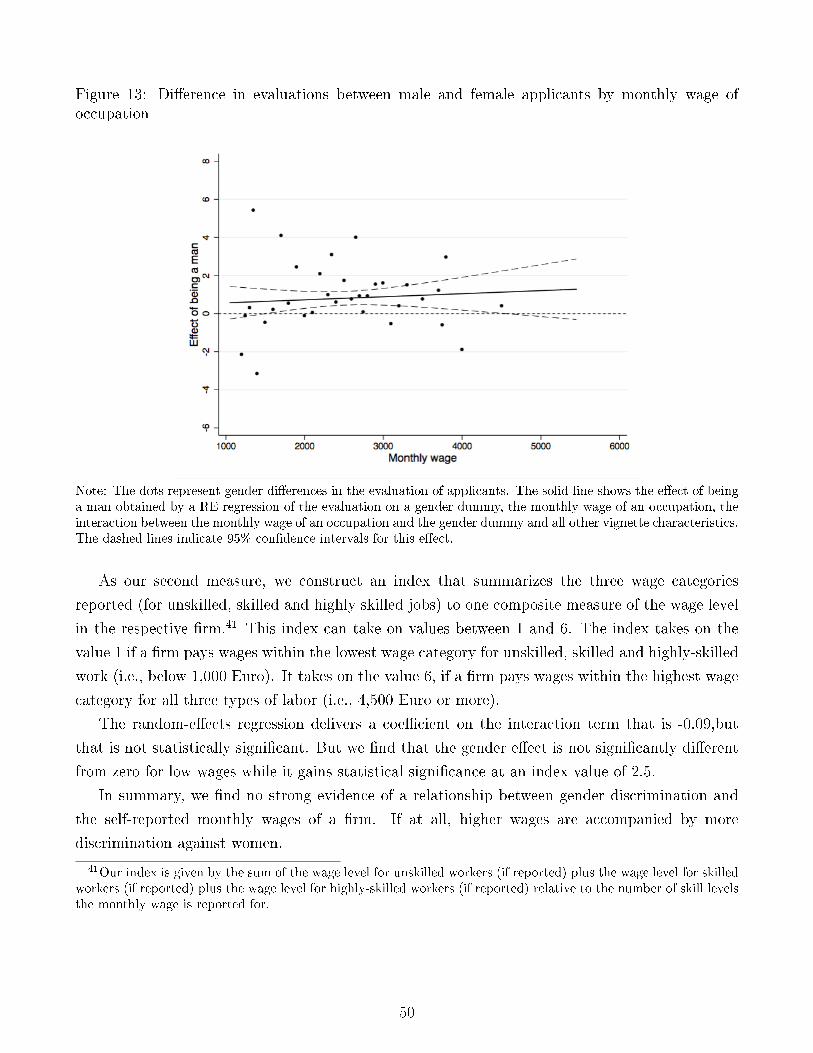
Figure 13: Di�erence in evaluations between male and female applicants by monthly wage ofoccupation
Note: The dots represent gender di�erences in the evaluation of applicants. The solid line shows the e�ect of beinga man obtained by a RE regression of the evaluation on a gender dummy, the monthly wage of an occupation, theinteraction between the monthly wage of an occupation and the gender dummy and all other vignette characteristics.The dashed lines indicate 95% con�dence intervals for this e�ect.
As our second measure, we construct an index that summarizes the three wage categories
reported (for unskilled, skilled and highly skilled jobs) to one composite measure of the wage level
in the respective �rm.41 This index can take on values between 1 and 6. The index takes on the
value 1 if a �rm pays wages within the lowest wage category for unskilled, skilled and highly-skilled
work (i.e., below 1,000 Euro). It takes on the value 6, if a �rm pays wages within the highest wage
category for all three types of labor (i.e., 4,500 Euro or more).
The random-e�ects regression delivers a coe�cient on the interaction term that is -0.09,but
that is not statistically signi�cant. But we �nd that the gender e�ect is not signi�cantly di�erent
from zero for low wages while it gains statistical signi�cance at an index value of 2.5.
In summary, we �nd no strong evidence of a relationship between gender discrimination and
the self-reported monthly wages of a �rm. If at all, higher wages are accompanied by more
discrimination against women.
41Our index is given by the sum of the wage level for unskilled workers (if reported) plus the wage level for skilledworkers (if reported) plus the wage level for highly-skilled workers (if reported) relative to the number of skill levelsthe monthly wage is reported for.
50

A.6 Educational requirements using an index
Instead of considering the most frequent school-leaving quali�cation, we now construct an index
based on the �rms' self-reported educational requirements. The index is equal to 3 if all apprentices
of the �rm in the apprenticeship occupation completed high school, it is equal to 0 if all apprentices
of the �rm in the apprenticeship occupation have no school-leaving quali�cation, and it takes on
values between 0 and 3 depending on the number of apprentices with each school-leaving quali-
�cation relative to the total number of apprentices.42 This measure of educational requirements
complements our previous measure in that it focuses on di�erences between �rms with respect to
their overall cohorts of apprentices.
Figure 14 plots the average di�erences in evaluations against the education index. The gen-
der di�erence in the evaluations seems to be most pronounced for �rms with lower educational
requirements for their apprentices.
Figure 14: Gender di�erence in evaluations by education index
Note: The dots represent gender di�erences in the evaluation of applicants. The solid line shows the e�ect of being aman obtained by a RE regression of the evaluation on a gender dummy, the education index, the interaction betweenthe education index and the gender dummy and all other vignette characteristics. The dashed lines indicate 95%con�dence intervals for this e�ect.
Controlling for the vignette characteristics, the correlation between discrimination against
women and the education level (as measured by the education index) is statistically not signi�cantly
di�erent from zero. The coe�cient on the gender-education interaction is positive, indicating that
42The index is given by (number of apprentices with no school-leaving quali�cation*0+number of appren-tices who completed secondary school only*1+number of apprentices who completed intermediary secondaryschool*2+number of apprentices who completed high school*3)/total number of apprentices.
51
higher educational requirements are accompanied by a smaller di�erence in evaluations between
male and female applicants, but it is insigni�cant. At the mean (median) of the index, there is
statistically and economically signi�cant discrimination amounting to 0.93 (0.91) points. Only
when the index approaches three, which means that almost all apprentices completed high school,
is the discrimination against women 0.52 and statistically not distinguishable from zero anymore.
A.7 Can salaries, educational requirements, and status explain discrim-
ination?
In order to investigate more thoroughly whether none of the status-related variables has explana-
tory power, we run a number of regressions where we only use one of the variables related to
status.
First, we include the average hourly wage along with the other moderator variables (the share
of female apprentices, the occupation type, �rm size, the number of steps in the recruitment
process), the interaction between the hourly wage and gender, the interaction between gender
and the moderators and other control variables in the RE regression (Table 4, column (3)). The
coe�cient on the wage-gender interaction is statistically insigni�cant. For the other moderator
variables the results are unchanged. There is a statistically signi�cant and positive in�uence of the
share of current female apprentices on the e�ect of being a female applicant. Increasing the share
of female apprentices by one standard deviation (0.32 percentage points) is associated with an
improvement in the evaluations of female applicants relative to the evaluation of male applicants
by 0.65 points. There is no statistically signi�cant in�uence on the e�ect of being female on
evaluations by �rm size, degree of professionalization nor type of occupation.
Second, we replace the hourly wage by the education index and introduce an interaction term
for the educational requirement and gender (Table 4, column (4)). The education-gender inter-
action term is economically and statistically not signi�cant. The coe�cient on the interaction
term between gender and the share of female apprentices increases slightly and remains highly
statistically signi�cant and sizeable.
Third, we subsequently include the ISEI and the SIOPS (Table 4, column (5) and column (6).
Again, we �nd no evidence that status (as measured by the ISEI or SIOPS), �rm size, occupation
type, or degree of professionalization in�uence gender-di�erences. The coe�cient on the interaction
term between gender and the share of female apprentices decreases slightly, but we still �nd a strong
e�ect of the share of currently employed female apprentices on the gender dummy.
52

All discussion papers are downloadable: http://www.wzb.eu/en/publications/discussion-papers/markets-and-choice
Discussion Papers of the Research Area Markets and Choice 2017
Research Unit: Market Behavior
Dorothea Kübler, Julia Schmid, Robert Stüber SP II 2017-201 Be a man or become a nurse: Comparing gender discrimination by employers across a wide variety of professions
Research Unit: Economics of Change
Jannis Engel, Nora Szech SP II 2017-301 The political economy of multilateral aid funds
Maja Adena, Jeyhun Alizade, Frauke Bohner, Julian Harke, Fabio Mesners
SP II 2017-302
Quality certifications for nonprofits, charitable giving, and donor’s trust: experimental evidence