Chapter 15: Quaternions: Multiplication in the Space of Mass-Points

Be fruitful and multiply Genesis 1:28

1. Vector Spaces and Division Algebras

The space of mass-points is a 4-dimensional vector space: addition, subtraction, and scalar multiplication are all well-defined operations on mass-points. But what about a more universal form of multiplication? Can we multiply together two points or more generally two mass-points?

In lower dimensional vector spaces, we can indeed multiply any two elements in the space. Every 1-dimensional vector space is isomorphic (equivalent) to the real number line. We can multiply any two points along the number line by the standard rules for multiplication of real numbers. Every 2-dimensional vector space is isomorphic to the plane. If we identify each pair of rectangular coordinates

�

(a,b) in the plane with the complex number

�

a + bi, then we can multiply two vectors in the plane using the standard rules for multiplication of complex numbers.

Vectors in 3-dimensions are endowed with two distinct products: dot product and cross product. The dot product of two vectors is a scalar; the cross product of two vectors is a vector. When we add or subtract two vectors, we get another vector. When we say that we want to multiply two vectors, we typically mean that we also want the result to be another vector. The dot product of two vectors is not a vector, so dot product is not the kind of multiplication that we seek. The cross product of two vectors is a vector; nevertheless cross product also has some undesirable properties. Multiplication is typically associative, commutative and distributes through addition. Moreover, in order to solve simple equations, we would like to have an identity for multiplication as well as multiplicative inverses (division). Although cross product distributes through addition, the cross product is neither associative nor commutative. Moreover there is no multiplicative identity for cross product -- that is, there is no vector u such that for all vectors v, we have

�

u ×v = v × u = v -- since by definition

�

u ×v⊥v . Hence there can be no multiplicative inverses for cross product. In fact, in 3-dimensions there is no entirely satisfactory notion of vector multiplication.

A division algebra (an algebra where we can perform division) is a set S where we can add, subtract, multiply, and divide any two elements in S. (One exception: we cannot divide by zero, the identity for addition.) Addition and multiplication must satisfy the usual rules: addition is associative and commutative; multiplication is associative and distributes through addition. Notice that we shall not insist that multiplication is commutative, since the multiplication that we have in mind for mass-points is not commutative. There is an identity 0 for addition and an identity 1 for multiplication so that for any element s in S

�

s + 0 = 0 + s = ss ⋅1= 1 ⋅ s = s.

Finally, for each element s in S, there is an inverse for addition

�

(−s) and an inverse for

multiplication

�

(s−1) so that

�

s + (− s) = (− s) + s = 0

�

s ⋅ s−1 = s−1 ⋅ s = 1 (s ≠ 0).Thus in a division algebra, we can subtract and divide, as well as add and multiply.

There are only three finite dimensional vector spaces that are also division algebras -- that is, there are only three dimensions in which we can define addition, subtraction, multiplication and division -- dimensions 1,2,4. These vector spaces correspond to the line (real numbers), the plane (complex numbers), and the space of mass-points (quaternions). (There is also a non-associative multiplication in dimension 8, the Cayley numbers or octonions.) We are really unbelievably lucky that Computer Graphics is grounded in the 4-dimensional vector space of mass-points.

In this chapter we shall define quaternion multiplication in the space of mass-points and investigate applications of quaternion multiplication to Computer Graphics. We will begin, however, with a simpler, better known paradigm: complex multiplication for vectors in the plane.

2. Complex Numbers

Complex numbers are low dimensional easy to understand analogues of the quaternions. Many of the fundamental algebraic and geometric properties of the quaternions appear as well in the complex numbers. One of the themes of this chapter is that many of the algebraic and geometric properties of the quaternions are easier to understand when reduced to the analogous properties of the complex numbers. With this kinship in mind, we begin our discussion of quaternions with a brief review of the complex numbers.

Complex numbers are often represented by vectors in 2-dimensions. The complex number w = a + bi corresponds to the vector v = (a,b) in the xy -plane. Addition, subtraction, and scalar multiplication of complex numbers correspond to coordinate-free operations on vectors in the plane. Rectangular coordinates are introduced in practice to perform these computations, but in principle there is no need for preferred directions -- for coordinate axes -- to define addition, subtraction, or scalar multiplication for vectors in the plane.

Complex multiplication is different. For complex multiplication we must choose a preferred direction: the direction of the identity vector for multiplication. We denote this identity vector by 1 and we associate this vector with the unit vector along the positive x-axis. The unit vector perpendicular to the identity vector we denote by i and we associate this vector with the unit vector along the positive y-axis. Relative to this coordinate system for every vector v in the plane there are

2

constants

�

a,b such that

�

v = a1+ bi .Typically we drop the symbol 1, and we write simply

�

v = a+ bi . (2.1)

In the complex number system, i denotes

�

−1 , so

�

i2 = −1. (2.2)Since 1 is the identity for multiplication, we have the rules

�

(1)(1) = 1,

�

(i)(1) = (1)(i) = i ,

�

(i)(i) = −1. (2.3)Therefore if we want complex multiplication to distribute through addition, then we must define

�

(a + b i)(c + d i) = a(c + d i) + bi(c + d i) = (ac − bd) + (ad + bc)i . (2.4)Using Equation (2.4), it is easy to verify that complex multiplication is associative, commutative, and distributes through addition (see Exercise 1).

Every non-zero complex number has a multiplicative inverse. Let

�

v = a+ bi . The complex conjugate of v, denoted by

�

v∗ , is defined by

�

v∗ = a− bi. (2.5)By equation (2.4)

�

v v∗ = a 2+ b2 = | v |2. (2.6)Therefore

�

v−1 =v∗

| v |2.

From Equations (2.4) and (2.5) it also is easy to verify that

(w1w2 )∗ = w1∗w2

∗ . (2.7)

Hence by Equations (2.6) and (2.7)

| w1 w2 | 2 = (w1w2 )(w1 w2 )∗ = (w1w1∗)(w2 w2

∗ ) = | w1 | 2 | w2 | 2 ,

so| w1 w2 | = | w1 | | w2 | . (2.8)

Equation (2.4) encapsulates the algebra of complex multiplication. But what is the geometry underlying complex multiplication?

To understand the geometry underlying complex multiplication, observe that multiplication by a fixed complex number w is a linear transformation on vectors in the plane, since by the distributive property

3

w(z1 + z2 ) = wz1 + wz2 .Moreover, multiplication by a complex number of unit length is an isometry (preserves length) because by Equation (2.8)

| w1 | = 1 ⇒ | w1 w2 | = | w2 | .But the only linear isometries in the plane are rotations, so multiplication by a complex number of length one must rotate vectors in the plane.

Let’s look at some examples. Consider first multiplication with i. If

�

v = a+ bi , then

�

i v = i(a + bi) = −b + ai .Thus if

�

v = (a,b), then

�

i v = (−b,a), so v ⋅ iv = (a,b) ⋅ (−b,a) = 0 .

Hence,

�

i v is perpendicular to v. Therefore multiplication by i is equivalent to rotation by

�

90 . Also,

�

(−1)v = −(a+ bi) = −a − bi = −v ,so multiplication by

�

−1 is equivalent to rotation by

�

180 . Thus there is indeed a link between rotation and complex multiplication. Let’s explore this connection further.

Recall from Chapter 4 that the matrix which rotates vectors in the plane by the angle

�

φ is given by:

�

rot(φ) =cos(φ) sin(φ)−sin(φ) cos(φ)⎛

⎝ ⎜

⎞

⎠ ⎟ .

Let

�

z = (x, y) = x + i y be an arbitrary vector in the plane. Then after rotation by the angle

�

φ

�

znew = z∗ rot(φ) = (x y) ∗cos(φ) sin(φ)−sin(φ) cos(φ)⎛

⎝ ⎜

⎞

⎠ ⎟ ,

or equivalently

�

xnew = x cos(φ) − y sin(φ)

�

ynew = x sin(φ) + y cos(φ).Now let

�

w(φ) be the unit vector that makes an angle

�

φ with the x-axis (see Figure 1). Then

�

w(φ) = cos(φ) + i sin(φ),

and

�

w(φ)z = cos(φ) + isin(φ)( ) x + i y( ) = x cos(φ) − y sin(φ)xnew

⎛

⎝

⎜ ⎜ ⎜

⎞

⎠

⎟ ⎟ ⎟

+ x sin(φ) + y cos(φ)ynew

⎛

⎝

⎜ ⎜ ⎜

⎞

⎠

⎟ ⎟ ⎟ i .

Thus multiplying the complex number z by

�

w(φ) is equivalent to rotating the vector z by the angle

�

φ . Moreover, since complex multiplication is associative, we can compose two rotations simply by 4

multiplying the associated complex numbers -- that is, for all z

�

w(φ +θ) z = w(φ) w(θ) z ,so

�

w(φ +θ) = w(φ) w(θ) .

Representing rotations in the plane by complex numbers is more efficient than matrix representations for rotations in the plane. To store one complex number, we need to store only two real numbers, whereas to store one

�

2 × 2 matrix, we need to store four real numbers. To compose two rotations by complex multiplication requires only 4 real multiplications, whereas to compose two rotations by matrix multiplication requires 8 real multiplications.

Rotation in the plane closely resembles exponentiation because composing two rotations is equivalent to adding the corresponding angles of rotation. Since complex multiplication represents rotation, complex multiplication is also closely related to exponentiation. Let z be an arbitrary complex number, and define

�

ez = 1+ z +z2

2!+

z3

3!+ .

Then

�

eiφ = 1+ iφ +(iφ) 2

2!+

(iφ) 3

3!+

(iφ)4

4!+

(iφ)5

5! .

But

�

i2 = −1, so substituting and collecting terms and then recalling the Taylor expansions of sine and cosine, we arrive at the following fundamental identity:

Euler’s Formula

�

eiφ = 1− φ2

2! +φ4

4! −⎛

⎝ ⎜

⎞

⎠ ⎟ + φ −

φ3

3! +φ5

5! −⎛

⎝ ⎜

⎞

⎠ ⎟ i = cos(φ) + isin(φ). (2.9)

Since

�

w(φ) = cos(φ) + i sin(φ) = eiφ ,we conclude that

�

w(φ)w(θ) = eiφeiθ = ei (φ+θ) = w(φ +θ) ,so multiplying two complex numbers of unit length is equivalent to adding the angles that these vectors form with the x-axis.

What happens if we multiply a fixed complex number z by an arbitrary complex number w? If

�

w = r , where r is a real number, then

�

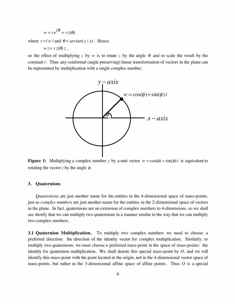
w z = rz , so the effect is to scale the vector z by the constant r. Thus both rotation and scaling can be represented by complex multiplication. Finally, if

�

w = x + i y is an arbitrary complex number, then we can write w in polar form as

5

�

w = reiθ = rz(θ)

where

�

r = | w | and

�

θ = arctan(y / x) . Hence

�

w z = rz(θ) z ,so the effect of multiplying z by w is to rotate z by the angle

�

θ and to scale the result by the constant r. Thus any conformal (angle preserving) linear transformation of vectors in the plane can be represented by multiplication with a single complex number.

�

y − axis

�

w = cos(φ )+ sin(φ ) i

�

•

�

φ

�

x − axis

Figure 1: Multiplying a complex number z by a unit vector

�

w = cos(φ) + sin(φ) i is equivalent to rotating the vector z by the angle

�

φ .

3. Quaternions

Quaternions are just another name for the entities in the 4-dimensional space of mass-points, just as complex numbers are just another name for the entities in the 2-dimensional space of vectors in the plane. In fact, quaternions are an extension of complex numbers to 4-dimensions, so we shall see shortly that we can multiply two quaternions in a manner similar to the way that we can multiply two complex numbers.

3.1 Quaternion Multiplication. To multiply two complex numbers we need to choose a preferred direction: the direction of the identity vector for complex multiplication. Similarly, to multiply two quaternions, we must choose a preferred mass-point in the space of mass-points: the identity for quaternion multiplication. We shall denote this special mass-point by O, and we will identify this mass-point with the point located at the origin, not in the 4-dimensional vector space of mass-points, but rather in the 3-dimensional affine space of affine points. Thus O is a special

6

mass-point with mass

�

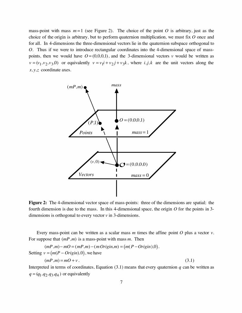
m = 1 (see Figure 2). The choice of the point O is arbitrary, just as the choice of the origin is arbitrary, but to perform quaternion multiplication, we must fix O once and for all. In 4-dimensions the three-dimensional vectors lie in the quaternion subspace orthogonal to O. Thus if we were to introduce rectangular coordinates into the 4-dimensional space of mass-points, then we would have

�

O = (0,0,0,1), and the 3-dimensional vectors v would be written as

�

v = (v1,v2,v3,0) or equivalently

�

v = v1i + v2 j + v3k , where

�

i, j, k are the unit vectors along the

�

x, y,z coordinate axes.

�

mass

�

Points

�

mass = 1

�

•

�

O = (0,0,0,1)

�

Vectors

�

mass = 0

�

•

�

O = (0,0,0,0)

�

•

�

(mP,m)

�

•

�

(P,1)

(v, 0)

Figure 2: The 4-dimensional vector space of mass-points: three of the dimensions are spatial; the fourth dimension is due to the mass. In this 4-dimensional space, the origin O for the points in 3-dimensions is orthogonal to every vector v in 3-dimensions.

Every mass-point can be written as a scalar mass m times the affine point O plus a vector v. For suppose that

�

(mP ,m) is a mass-point with mass m. Then

�

(mP ,m)− mO = (mP,m) − (mOrigin,m) = m(P −Origin),0( ) .Setting

�

v = m(P − Origin),0( ) , we have

�

(mP ,m) = mO + v . (3.1)Interpreted in terms of coordinates, Equation (3.1) means that every quaternion q can be written as

�

q = (q1,q2,q3,q4 ) or equivalently

7

�

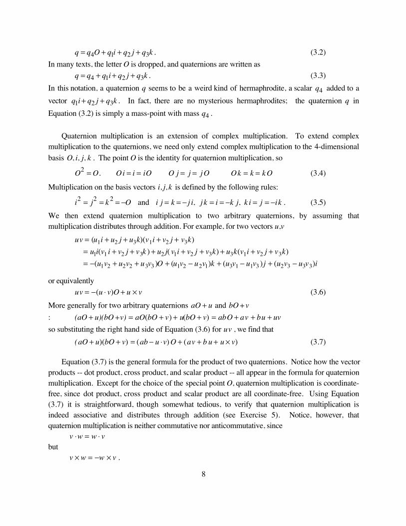
q = q4O + q1i + q2 j + q3k . (3.2)In many texts, the letter O is dropped, and quaternions are written as

�

q = q4 + q1i + q2 j + q3k . (3.3)In this notation, a quaternion q seems to be a weird kind of hermaphrodite, a scalar

�

q4 added to a vector

�

q1i + q2 j + q3k . In fact, there are no mysterious hermaphrodites; the quaternion q in Equation (3.2) is simply a mass-point with mass

�

q4 .

Quaternion multiplication is an extension of complex multiplication. To extend complex multiplication to the quaternions, we need only extend complex multiplication to the 4-dimensional basis

�

O, i, j, k . The point O is the identity for quaternion multiplication, so

�

O2 = O.

�

Oi = i = iO

�

O j = j = j O

�

Ok = k = k O (3.4)

Multiplication on the basis vectors

�

i, j, k is defined by the following rules:

�

i2 = j2 = k 2 = −O and

�

i j = k = − j i, j k = i = −k j, k i = j = −ik . (3.5)We then extend quaternion multiplication to two arbitrary quaternions, by assuming that multiplication distributes through addition. For example, for two vectors u,v

uv = (u1i + u2 j + u3k)(v1i + v2 j + v3k)    = u1i(v1 i + v2 j + v3k ) + u2 j( v1i + v2 j + v3k) + u3k(v1i + v2 j + v3k)    = −(u1v2 + u2v2 + u3v3 )O + (u1v2 − u2v1)k + (u3v1 − u1v3 ) j + (u2v3 − u3v3)i

or equivalentlyuv = −(u ⋅ v)O + u × v (3.6)

More generally for two arbitrary quaternions

�

aO + u and

�

bO+v:

�

(aO + u)(bO+v) = aO(bO + v) + u(bO + v) = abO + av + bu + uvso substituting the right hand side of Equation (3.6) for uv , we find that

�

(aO + u)(bO + v) = (ab − u ⋅v) O + (av + b u + u × v) (3.7)

Equation (3.7) is the general formula for the product of two quaternions. Notice how the vector products -- dot product, cross product, and scalar product -- all appear in the formula for quaternion multiplication. Except for the choice of the special point O, quaternion multiplication is coordinate-free, since dot product, cross product and scalar product are all coordinate-free. Using Equation (3.7) it is straightforward, though somewhat tedious, to verify that quaternion multiplication is indeed associative and distributes through addition (see Exercise 5). Notice, however, that quaternion multiplication is neither commutative nor anticommutative, since

v ⋅w = w ⋅ vbut

v × w = −w × v .

8

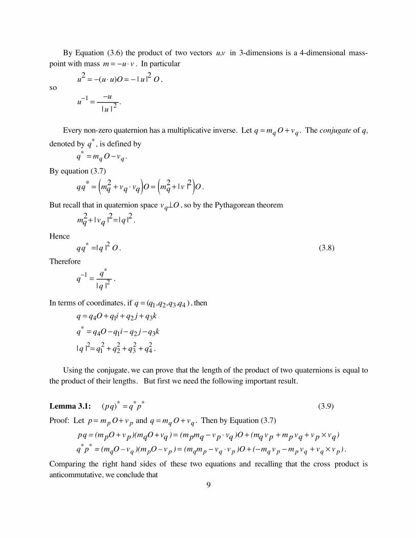
By Equation (3.6) the product of two vectors

�

u,v in 3-dimensions is a 4-dimensional mass-point with mass

�

m = −u ⋅ v . In particular

�

u2 = −(u ⋅ u)O = − | u |2 O ,so

�

u−1 =−u| u | 2 .

Every non-zero quaternion has a multiplicative inverse. Let

�

q = mq O + vq . The conjugate of q,

denoted by

�

q∗ , is defined by

�

q∗ = mq O −vq .

By equation (3.7)

�

qq∗ = mq2 + vq ⋅ vq( )O = mq

2 + | v |2( )O .

But recall that in quaternion space

�

vq⊥O , so by the Pythagorean theorem

�

mq2+ | vq |2= | q |2.

Hence

�

qq∗ =| q |2 O . (3.8)Therefore

�

q−1 =q∗

| q |2.

In terms of coordinates, if

�

q = (q1,q2,q3,q4 ), then

�

q = q4O + q1i + q2 j + q3k

�

q∗ = q4O −q1i− q2 j −q3k

�

| q |2= q12 + q2

2 + q32 + q4

2 .

Using the conjugate, we can prove that the length of the product of two quaternions is equal to the product of their lengths. But first we need the following important result.

Lemma 3.1:

�

(pq)∗ = q∗p∗ (3.9)

Proof: Let

�

p = mp O + v p and

�

q = mq O + vq . Then by Equation (3.7)

�

pq = (mpO + v p)(mqO+vq ) = (mpmq − v p ⋅ vq )O + (mq v p + mp vq + v p × vq)

�

q∗p∗ = (mqO – vq )(mpO – v p ) = (mqmp − vq ⋅v p )O + (−mq v p − mp vq + vq × v p) .

Comparing the right hand sides of these two equations and recalling that the cross product is anticommutative, we conclude that

9

�

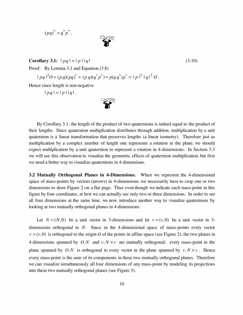
(pq)∗ = q∗p∗ .

Corollary 3.1: | pq | = | p | | q | (3.10)Proof: By Lemma 3.1 and Equation (3.8)

| pq |2O = (p q)(pq)∗ =  (p q)(q∗p∗ ) = p(q q∗)p∗ = | p |2  | q | 2 O .

Hence since length is non-negative| pq | = | p | | q | .

By Corollary 3.1, the length of the product of two quaternions is indeed equal to the product of their lengths. Since quaternion multiplication distributes through addition, multiplication by a unit quaternion is a linear transformation that preserves lengths (a linear isometry). Therefore just as multiplication by a complex number of length one represents a rotation in the plane, we should expect multiplication by a unit quaternion to represent a rotation in 4-dimensions. In Section 3.3 we will use this observation to visualize the geometric effects of quaternion multiplication, but first we need a better way to visualize quaternions in 4-dimensions.

3.2 Mutually Orthogonal Planes in 4-Dimensions. When we represent the 4-dimensional space of mass-points by vectors (arrows) in 4-dimensions, we necessarily have to crop one or two dimensions to draw Figure 2 on a flat page. Thus even though we indicate each mass-point in this figure by four coordinates, at best we can actually see only two or three dimensions. In order to see all four dimensions at the same time, we now introduce another way to visualize quaternions by looking at two mutually orthogonal planes in 4-dimensions.

Let N = (N ,0) be a unit vector in 3-dimensions and let v = (v, 0) be a unit vector in 3-dimensions orthogonal to N. Since in the 4-dimensional space of mass-points every vector v = (v, 0) is orthogonal to the origin O of the points in affine space (see Figure 2), the two planes in 4-dimensions spanned by O,N and v, N × v are mutually orthogonal: every mass-point in the plane spanned by O,N is orthogonal to every vector in the plane spanned by v, N × v . Hence every mass-point is the sum of its components in these two mutually orthogonal planes. Therefore we can visualize simultaneously all four dimensions of any mass-point by modeling its projections into these two mutually orthogonal planes (see Figure 3).

10

N

O

N × v

v

(a) the plane of O, N (b) the plane perpendicular to O, N

Figure 3: A mass-point represented by its projections (arrows) into two mutually orthogonal planes in 4-dimensions.

Although Figure 3 depicts two planes in 4-dimensions, the geometric interpretations of these two planes in terms of mass-points are markedly different: the plane perpendicular to O, N represents a plane of vectors in 3-dimensions, but in 3-dimensions the plane of O, N represents a line of points.

Consider first the plane perpendicular to O, N. Since the vectors v and N × v are orthogonal, the plane in 4-dimensions of the vectors

w = a v + b N × v

spanned by v, N × v represents the plane of 3-dimensional vectors perpendicular to N (see Figure 4).

v

N × vαv + βN × v

Figure 4: The plane of vectors perpendicular to O, N in 4-dimensions is the plane of vectors in 3-11

dimensions perpendicular to N. This plane is spanned by the vectors v and N × v , where v is any nonzero vector in 3-dimensions perpendicular to N.

On the other hand, consider the plane of O, N. In 3-dimensions O represents a point, not a vector. Thus the plane of 4-dimensional vectors

P = cO + s N

spanned by O,N actually represents a line in 3-dimensions: the line through the affine point O in the direction of the unit vector N. We shall write

(m P, m) ≡ (P,1)to denote that (m P, m) and (P,1) have the same location. Thus

P ≡ O +sc

N

-- that is, P is a mass-point with mass m = c on the line P(t ) = O + t N . (If c = 0 , then P is a vector sN parallel to the line P(t ) .) The plane spanned by O,N does have two dimensions, but only one dimension is spatial; the other dimension, the coefficient of O, represents mass not length (see Figure 5).

O

N

αO + βN

O

N

αO + βN ≡O +βα

N•

•x y

z

(a) a plane of vectors in 4-dimensions (b) a line of points in 3-dimensions.

Figure 5: (a) The plane of vectors (mass-points) in 4-dimensions spanned by O, N is equivalent to (b) the line of affine points in 3-dimensions passing through the point O in the direction of the vector N. This line is actually 2-dimensional, but the second dimension is mass-like not spatial, so this dimension is not visible in (b).

In addition to this geometric distinction, there is also an algebraic distinction between these two mutually orthogonal planes in 4-dimensions. We shall see in Section 3.3 that the plane of O, N is isomorphic algebraically to the complex numbers C, whereas the plane perpendicular to O, N is

12

isomorphic not to C but to Cv , where v is any unit vector perpendicular to N. We are going to take advantage of these asymmetries in the algebraic and geometric properties of these two mutually orthogonal planes in 4-dimensions in Section 3.4 when we study conformal transformations on points and vectors in 3-dimensions based on quaternion multiplication.

3.3 The Geometry of Quaternion Multiplication. We want to see what happens when we multiply an arbitrary quaternion p by a unit quaternion

q(N ,θ ) = cos(θ) O + sin(θ )N ,where N is a unit vector and O is the identity for quaternion multiplication. There is one key algebraic insight that will allow us to visualize the geometric effects of this quaternion multiplication: For every unit vector N, the plane of O, N is isomorphic to the complex plane.

Indeed by Equation (3.6) for any unit vector N, we have

N2 = −O . Since

O2 = O , O N = N O = N , and N ⊥ O ,

multiplication in the plane determined by the two quaternions O,N behaves exactly like multiplication in the complex plane. Therefore, just as multiplication by the complex number

eiθ = cos(θ )+ sin(θ ) irotates vectors in the complex plane by the angle θ (see Section 2), multiplication by the unit quaternion

q(N ,θ ) = cos(θ) O + sin(θ )N

rotates quaternions in the plane of O,N by the angle θ (see Figure 6).

N

N − axis   

OO − axis   θ

q(N ,θ ) = cos(θ )O +sin(θ ) Ni

y− axis    

1x − axis   

eiθ = cos(θ ) + sin(θ) i

θ

(a) the quaternion plane of O, N (b) the complex plane

13

Figure 6: For any unit vector N: (a) the plane determined by O, N is isomorphic algebraically and homeomorphic geometrically to (b) the complex plane: O ↔1 and N ↔ i , since O2 = O , N2 = −O , O N = N O = N , and N ⊥ O . Hence

q(N ,θ ) = cos(θ) O + sin(θ ) N ↔ eiθ = cos(θ ) + sin(θ) i .

Therefore we have the following results.

Lemma 3.2: Let N be a unit vector. Theni. q(N , θ ) q(N , φ) = q(N , θ +φ)

ii. q(N , θ ) q(N , φ) = q(N , φ ) q(N, θ)Proof: To prove i, we simply apply quaternion multiplication -- Equation (3.7) -- and the trigonometric identities for the sine and the cosine of the sum of two angles:

i.   q(N , θ ) q(N, φ) = cos(θ)O + sin(θ) N( ) cos(φ)O + sin(φ)N( )       = cos(θ )cos(φ) − sin(θ)sin(φ)( )O + sin(θ )cos(φ) + cos(θ )sin(φ)( ) N

                                  = cos(θ + φ)O + sin(θ + φ)N                                  = q(N , θ +φ) .ii. Follows immediately from i.

Since multiplying arbitrary quaternions by a fixed unit quaternion is a linear isometry in 4-dimensions, unit quaternions q(N ,θ ) represent rotations in 4-dimensions. By Lemma 3.2 we

understand how q(N ,θ ) rotates quaternions in the plane determined by O,N because in this plane

multiplication by q(N ,θ ) behaves just like multiplication by eiθ in the complex plane. But to fully

visualize how multiplication by q(N ,θ ) affects arbitrary quaternions, we still need to see how

q(N ,θ ) affects quaternions in the complementary plane of quaternions perpendicular to O,N .

In facilitate our presentation, we now introduce the following notation:Lq ( p) = q p left multiplication by q

Rq( p) = p q right multiplication by q

Sq (p) = q pq∗ = Lq Rq∗ ( p)( ) sandwiching p between q and q∗ .The functions Lq ( p) and Rq( p) are linear transformations on the vector space of quaternions

because quaternion multiplication distributes through quaternion addition. The sandwiching

14

operator Sq (p) is also a linear transformations because Sq (p) is the composite of two linear

transformations. We shall see in Section 3.4 that the sandwiching operator Sq (p) plays a central

role in the use of quaternions for computing rotations in 3-dimensions.

We are now ready to study the geometric effects of multiplication by the unit quaternionsq(N ,θ ) = cos(θ) O + sin(θ )N

q∗ (N ,θ ) = cos(θ )O − sin(θ )N = q(N ,−θ) (3.11)

on quaternions in the plane of O, N -- which we have already seen is isomorphic to the complex plane -- and on quaternions in the complementary plane of vectors perpendicular to O, N.

Proposition 3.2: Rotation in the Plane of O, NLet• N = a unit vector• p = a quaternion in the plane of O, NTheni. Lq( N , θ )(p) = q(N ,θ) p rotates p by the angle θ in the plane of O, N

ii. Rq(N ,θ )(p) = p q(N ,θ) rotates p by the angle θ in the plane of O, N

iii. Rq∗ (N ,θ) p = p q∗ (N , θ) rotates p by the angle −θ in the plane of O, N

iv. Sq( N ,θ)( p) = q(N , θ) p q∗ (N , θ ) is the identity on p.

Proof: i, ii. Follow immediately from Lemma 3.2..iii. Follows immediately from ii and Equation (3.11)iv. Follows immediately from i and iii. .

Proposition 3.3: Rotation in the Plane Perpendicular to O, NLet• N = a unit vector• v = a vector in the plane ⊥ O, NTheni. Lq( N ,θ )(v) = q(N ,θ) v rotates v by the angle θ in the plane ⊥ O, N

ii. Rq(N , θ )(v) = v q(N ,θ) rotates v by the angle −θ in the plane ⊥ O, N

iii. Rq∗ (N , θ)(v) = v q∗(N ,θ ) rotates v by the angle θ in the plane ⊥ O, N

iv. Sq( N , θ)(v) = q(N ,θ) v q∗ (N ,θ ) rotates v by the angle 2θ in the plane ⊥ O, N.

15

Proof: Since v ⊥ N , it follows that v ⋅N = 0 . Hence, by Equation (3.6), N v = N × v and v N = v × N . Therefore:

i. q(N ,θ ) v = cos(θ)O + sin(θ) N( )v = cos(θ)v + sin(θ) N × v

ii. v q(N ,θ ) = v cos(θ )O + sin(θ )N( ) = cos(θ )v + sin(θ )v× N = cos(θ)v − sin(θ) N × v

iii. v q∗(N ,θ ) = v cos(θ )O −sin(θ )N( ) = cos(θ )v− sin(θ )v × N = cos(θ)v + sin(θ )N × v

Equations i and iii represent rotation by the angle θ and Equation ii represents rotation by the angle −θ in the plane perpendicular to O, N (see Figure 7). Now it follows easily from i and iii that

multiplication by q(N ,θ ) on the left and multiplication by q∗ (N ,θ ) on the right both rotate vectors

v in the plane perpendicular to O, N by the same angle θ . Therefore

iv. q(N ,θ ) v q∗(N, θ) rotates v by the angle 2θ in the plane ⊥ O, N.

�

N × v

�

v

�

(cosθ )v

�

(sinθ) N × v

�

θ�

q(N , θ)v

�

−θ

�

−(sinθ )N × v

�

v q(N , θ)

Figure 7: Rotation by the angle ±θ in the plane ⊥ O, N.

Propositions 3.2 are 3.3 are summarized graphically in Figure 8 and 9. These two figures encapsulate geometrically the main properties of quaternion multiplication presented in this section.

16

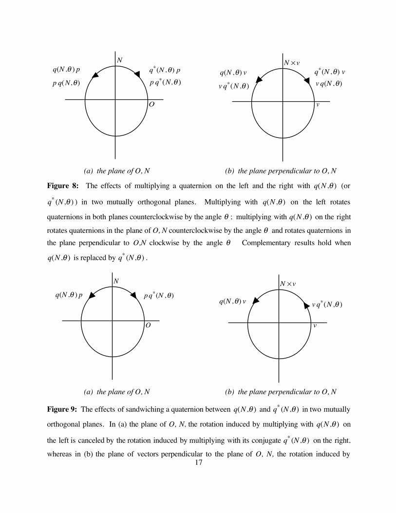
N

O

N × v

v

q(N ,θ ) p

p q( N,θ) p q∗(N,θ )q(N ,θ) v

v q(N ,θ)v q∗(N ,θ )

q∗(N ,θ) p q∗(N ,θ) v

(a) the plane of O, N (b) the plane perpendicular to O, N

Figure 8: The effects of multiplying a quaternion on the left and the right with q(N ,θ ) (or

q∗ (N ,θ ) ) in two mutually orthogonal planes. Multiplying with q(N ,θ ) on the left rotates

quaternions in both planes counterclockwise by the angle θ ; multiplying with q(N ,θ ) on the right

rotates quaternions in the plane of O, N counterclockwise by the angle θ and rotates quaternions in the plane perpendicular to O,N clockwise by the angle θ Complementary results hold when

q(N ,θ ) is replaced by q∗ (N ,θ ) .

N

O

N × v

v

q(N ,θ ) p pq∗(N ,θ)q(N ,θ) v v q∗(N ,θ )

(a) the plane of O, N (b) the plane perpendicular to O, N

Figure 9: The effects of sandwiching a quaternion between q(N ,θ ) and q∗ (N ,θ ) in two mutually

orthogonal planes. In (a) the plane of O, N, the rotation induced by multiplying with q(N ,θ ) on

the left is canceled by the rotation induced by multiplying with its conjugate q∗ (N ,θ ) on the right,

whereas in (b) the plane of vectors perpendicular to the plane of O, N, the rotation induced by 17

multiplying with q(N ,θ ) on the left is reinforced by the rotation induced by multiplying with its

conjugate q∗ (N ,θ ) on the right.

With this introduction to quaternion algebra and geometry in 4-dimensions, we are finally ready to turn our attention to the main applications of quaternion multiplication in Computer Graphics: computing conformal transformations on points and vectors in 3-dimensions.

3.4 Quaternion Representations for Conformal Transformations. Quaternion multiplication can be used to model rotations of vectors in 3-dimensions much like complex multiplication can be used to model rotations of vectors in the plane. In fact, quaternion multiplication can be used to model any conformal transformation -- rotation, mirror image, and uniform scaling -- of vectors in 3-dimensions.

The key to modeling conformal transformations with quaternions is the sandwiching map

�

Sq(v) = q v q∗ .

Notice that

�

(S p Sq)(v) = Spq(v) (3.12)because by Lemma 3.1

�

(S p Sq)(v) = Sp Sq(v)( ) = S p q v q∗( ) = p q v q∗p∗ = (p q) v (pq)∗ = Spq(v) .

Proposition 3.4: Let

�

q(N ,φ) = cos(φ / 2)O + sin(φ / 2)N . Then a vector v can be rotated around

the axis N through the angle

�

φ by sandwiching v between

�

q(N ,φ) and

�

q(N ,φ)∗ .

Proof: Let v = v + v⊥ , where

• v = component of v parallel to N

• v⊥ = component of v perpendicular to N.Then

• Sq( N ,θ /2)(v) = v (Proposition 3.2)

• Sq( Nθ / 2)(v⊥) rotates v⊥ by the angle θ in the plane ⊥ to O, N. (Proposition 3.3)

Therefore Sq( N ,θ /2)(v) has the same effect on the components of v as rotating v in 3-dimensions by

the angle θ around the axis vector N (see Chapter 12, Section 12.3.2).

18

Notice that the quaternion

�

q(N ,φ) is a unit quaternion because by Equation (3.8)

�

q(N,φ) 2O = q(N,φ)q(N ,φ)∗ = cos2(φ / 2) + sin2(φ / 2)( )O = O .

Thus every rotation is represented by a unit quaternion. Conversely, every unit quaternion

represents a rotation because if

�

q = mq O + vq is a unit quaternion, then

�

mq2 + | vq |2 = 1. Hence there

is an angle

�

θ and a unit vector N such that

�

mq = cos(θ) and

�

vq = sin(θ)N , so

�

q = cos(θ)O + sin(θ)N = q(N ,θ).

To model mirror image with sandwiching, observe that to find the mirror image of a vector v in

the plane perpendicular to the unit normal vector N, we can rotate v by

�

1800 around N and then negate the result. Now

�

q(N ,π / 2) = cos(π / 2)O + sin(π / 2)N = N .Thus to rotate v by

�

1800 around N, we can sandwich v between N and

�

N∗ . Since for vectors

�

N∗ = −N , it follows that mirror image of v in the plane perpendicular to N is given by

�

−SN (v) = N v N .Thus we are led to the following result.

Proposition 3.5: A vector v can be mirrored in the plane perpendicular to the unit normal N by sandwiching v between two copies of N.Proof: Let

v = v + v⊥ , where

• v = component of v parallel to N

• v⊥ = component of v perpendicular to N.

Since N = cos(π / 2)O + sin(π / 2)N = q(N ,π / 2) :

• −S N (v) = −Sq(N , π /2) (v ) = −v (Proposition 3.2)

• −S N (v⊥ ) = −Sq( N ,π /2)(v⊥ ) = v⊥ (Proposition 3.3)

Hence sandwiching v between two copies of N has the same effect on the components of v as mirroring v in 3-dimensions in the plane perpendicular to N (see Chapter 12, Section 12.3.3).

Proposition 3.6: A vector v can be scaled by the factor c by sandwiching v between two copies of

�

c O.Proof:

�

S c O(v) = c O v c O = c v .

19

Theorem 3.1: Every conformal transformation of vectors in 3-dimensions can be modeled by sandwiching with a single quaternion.Proof: This result follows from Propositions 3.4-3.6, since by Equation (3.12) composition of sandwiching is equivalent to multiplication of quaternions.

Conformal transformations of vectors in 3-dimensions can be computed by sandwiching the vectors with the appropriate quaternions. But what about conformal transformations on points in 3-dimensions? To rotate points about arbitrary lines, or to mirror points in arbitrary planes, or to scale points uniformly about arbitrary points, we cannot simply sandwich the points we wish to transform with some appropriate quaternion (see Exercises 11 and 15). Recall, however, that rotation, mirror image, and uniform scaling, all have a fixed point Q of the transformation. Since

�

P = Q + (P −Q) , we can compute conformal transformations on affine points P by using quaternions to transform the vectors

�

P −Q and then adding the resulting vectors to Q. In this way, quaternions can be applied to compute conformal transformations on points as well as on vectors.

3.5 Quaternions vs. Matrices. We now have two ways to represent conformal transformations on vectors in 3-dimensions:

�

3× 3 matrices and quaternions. Here we shall compare and contrast some of the advantages and disadvantages of quaternion and matrix representations for conformal transformations.

A

�

3× 3 matrix contains 9 scalar entries, whereas a quaternion can be represented by 4 rectangular coordinates. Thus if memory is at a premium, quaternions are more than twice as efficient as matrices. On the other hand, by Equation (3.7) to compute the product of two quaternions requires 16 real scalar multiplications: 6 for the cross product, 3 for the dot product, 6 for the two scalar products, and one for the product of the two scalar masses. Similarly, since a vector has zero mass, the product of a quaternion and a vector requires 12 scalar multiplications, since the product of the masses as well as one of the scalar products is zero. Sandwiching a vector with a quaternion computes a product of a quaternion with a vector followed by the product of a quaternion with a quaternion, so the total cost for one conformal transformation using quaternions is

�

12 + 16 = 28 scalar multiplications, whereas the cost for multiplying a vector by a

�

3× 3 matrix is only 9 scalar multiplications. Thus matrices are more than 3 times as fast as quaternions for computing arbitrary conformal transformations. But there is also an additional computational consideration. To compose two transformations by quaternion multiplication requires 16 scalar multiplications, whereas to compose two transformations by matrix multiplication requires 27 scalar multiplications. Therefore quaternion multiplication is more than 1.5 times faster than matrix multiplication for composing conformal transformations. Thus some computations favor quaternions, whereas others favor matrices. We summarize these tradeoffs for both memory and speed in Table 1.

20

memory transformation composition

quaternions 4 scalars 28 multiplies 16 multiplies

�

3× 3 matrices 9 scalars 9 multiplies 27 multiplies

Table 1: Tradeoffs between speed and memory for quaternions and

�

3× 3 matrices.

3.6 Avoiding Distortion. Aside from considerations of memory and speed, one of the main advantages of quaternions over matrices is avoiding distortions that arise from numerical inaccuracies that are inevitably introduced by floating point computations.

For any

�

3× 3 matrix A representing an affine transformation,

�

inewjnewknew

⎛

⎝

⎜ ⎜

⎞

⎠

⎟ ⎟

=ijk

⎛

⎝

⎜ ⎜

⎞

⎠

⎟ ⎟ ∗A .

Since the matrix with rows

�

i, j, k is the identity matrix, we conclude that

�

A =inewjnewknew

⎛

⎝

⎜ ⎜ ⎜

⎞

⎠

⎟ ⎟ ⎟ . (3.13)

Hence the rows of A represent the images of the unit vectors

�

i, j, k along the coordinate axes.

Thus if a

�

3× 3 matrix A represents a conformal transformation, then the rows of A must be mutually orthogonal vectors, since conformal transformations preserve angles and the original vectors

�

i, j, k are mutually orthogonal. To compose conformal transformations, we must multiply matrices. But the entries of these matrices -- especially rotation matrices which contain values of sines and cosines -- are typically represented by floating point numbers. Therefore after composing several conformal transformations, the rows of the product matrix will no longer be mutually orthogonal vectors due to numerical inaccuracies introduced by floating point computations. Thus these matrices no longer represent conformal transformations, so applying these matrices will distort angles in the image.

Quaternions avoid this problem. To compose conformal transformations, we multiply the corresponding quaternions. Since every quaternion represents a conformal transformation, computing transformations by sandwiching with quaternions will never distort angles.

Suppose, however, that we want to compose only rotations. Composing rotations by matrix multiplication will generate distortions in both lengths and angles due to numerical inaccuracies introduced by floating point computations. We need to renormalize the resulting matrix so that the rows are mutually orthogonal unit vectors, but it is not clear how to perform this normalization.

21

This normalization, however, is easy to perform with quaternions. Rotations are represented by unit quaternions. When we compose rotations by multiplying unit quaternions, the result may no longer be a unit quaternion due to floating point computations. But we can normalize the resulting quaternion q simply by dividing by its length

�

| q |. The resulting quaternion

�

q/ | q | is certainly a unit quaternion, so this normalization avoids distorting either lengths or angles in the image.

3.7 Key Frame Animation. Quaternions have one additional advantage over matrices: quaternions can be used to interpolate in between frames for key frame animation. In key frame animation, an artist draws only a few key frames in the scene, and an animator must interpolate intermediate frames to make the animation look natural.

Consider an object tumbling through a scene. An artist will typically draw only a few frames representing rotations of the object at certain key times. An animator must then find intermediate rotations, so that the tumbling appears smooth. Suppose that from the artist’s drawing we know the rotations

�

R0 and

�

R1 at times

�

t = 0 and

�

t = 1. How do we find the appropriate intermediate rotations at intermediate times?

If the rotations

�

R0,R1 are represented by

�

3× 3 matrices, then we seek intermediate rotation matrices

�

R(t) for

�

0 < t < 1. We might try linear interpolation and set

�

R(t) = (1− t)R0 + t R1.The problem with this approach is that the matrices

�

R(t) are no longer rotation matrices because the rows of these matrices are no longer mutually orthogonal unit vectors. Thus the matrices

�

R(t) will introduce undesirable distortions into the animation.

Alternatively, we could use unit quaternions

�

q0,q1 to represent these two rotations. The quaternion generated by linear interpolation

�

q(t) = (1− t)q0 + t q1is no longer a unit quaternion, but we can adjust the length of

�

q(t) by dividing by

�

| q(t) |. Now

�

q(t)/ | q(t) | is a unit quaternion representing an intermediate rotation. Unfortunately, the tumbling motions generated by this approach will not appear smooth because linear interpolation does not generate uniformly spaced quaternions -- that is, if

�

φ is the angle between

�

q0 and

�

q1, then

�

tφ is not generally the angle between

�

q0 and

�

q(t)/ | q(t) |.

To correct for this problem, we apply spherical linear interpolation (SLERP, see Chapter 11, Section 11.6) -- that is, we set

�

q(t) = slerp(q0,q1,t) =sin (1− t)φ( )

sin(φ)q0 +

sin tφ( )sin(φ)

q1, (3.14)

22

where

�

φ is the angle between

�

q0 and

�

q1. Recall that SLERP guarantees that if

�

q0 and

�

q1 are unit quaternions, then

�

q(t) is also a unit quaternion, and if

�

φ is the angle between

�

q0 and

�

q1, then

�

tφ is the angle between

�

q0 and

�

q(t) . Thus spherical linear interpolation applied to quaternions generates the appropriate intermediate rotations for key frame animation.

3.8 Conversion Formulas. Since we have two ways to represent conformal transformations on vectors in 3-dimensions --

�

3× 3 matrices and quaternions -- and since each of these representations is superior for certain applications, it is natural to develop formulas to convert between these two representations. If a quaternion represents scaling along with rotation, the scale factor can be retrieved from the magnitude of the quaternion. Similarly if a

�

3× 3 matrix is a composite of rotation and uniform scaling, the scale factor can be retrieved from the determinant of the matrix. Therefore we can easily retrieve these scale factors, and we can always normalize quaternions to have unit length and conformal matrices to have unit determinant. Unit quaternions and

�

3× 3 conformal matrices with unit determinant represent rotations. Since, as we have just seen in Sections 3.3 and 3.4, rotations embody the most important applications of quaternions to Computer Graphics, we will concentrate here on converting between different representations for rotations.

Consider a rotation around the unit axis vector N by the angle

�

φ . The rotation matrix (Chapter 13, Section 13.3.2) and the unit quaternion (Section 3.2, Proposition 2) that represent this rotation are given by

�

Rot(N ,φ) = (cosφ) I + (1− cosφ)( NT ∗N) + (sinφ)(N × _) (3.15)

�

q(N ,φ / 2) = cos(φ / 2)O + sin(φ / 2)N . (3.16)To convert between these two representations for rotation, we shall make extensive use of the following half angle and double angle formulas for sine and cosine (see Exercise 3):

�

cos2 φ / 2( ) =1+ cosφ

2

�

sin2(φ / 2) =1− cosφ

2

�

sin(φ) = 2sin(φ / 2)cos(φ / 2)

Suppose that we are given the rotation matrix

�

Rot(N ,φ) = (cosφ) I + (1− cosφ)( NT ∗N) + (sinφ)(N × _) = (Ri , j )

and we want to find the corresponding unit quaternion

�

q(N ,φ / 2) = cos(φ / 2)O + sin(φ / 2)N . Then we need to find

�

cos(φ / 2) and

�

sin(φ / 2)N . Expanding Equation (3.15) in matrix form yields:

23

�

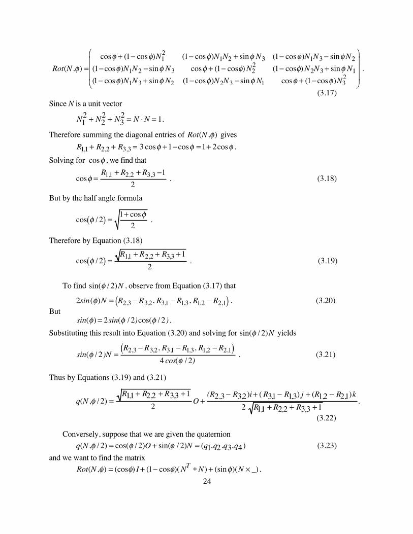
Rot(N ,φ) =cosφ + (1− cosφ)N1

2 (1− cosφ)N1N2 + sinφ N3 (1− cosφ)N1N3 − sinφN2(1−cosφ)N1N2 − sinφ N3 cosφ + (1− cosφ) N2

2 (1− cosφ) N2N3 + sinφ N1(1− cosφ)N1N3 + sinφ N2 (1−cosφ)N2N3 − sinφ N1 cosφ + (1−cosφ)N3

2

⎛

⎝

⎜ ⎜ ⎜

⎞

⎠

⎟ ⎟ ⎟ .

(3.17)Since N is a unit vector

�

N12 + N2

2 + N32 = N ⋅N = 1.

Therefore summing the diagonal entries of

�

Rot(N ,φ) gives

�

R1,1 + R2,2 + R3,3 = 3 cosφ + 1−cosφ = 1+ 2cosφ .Solving for

�

cosφ , we find that

�

cosφ =R1,1 + R2,2 + R3,3 −1

2 . (3.18)

But by the half angle formula

�

cos φ / 2( ) =1+ cosφ

2 .

Therefore by Equation (3.18)

�

cos φ / 2( ) =R1,1 + R2,2 + R3,3 + 1

2 . (3.19)

To find

�

sin(φ / 2)N , observe from Equation (3.17) that

�

2sin(φ)N = R2,3 − R3,2, R3,1 − R1,3, R1,2 − R2,1( ) . (3.20)But

�

sin(φ) = 2sin(φ / 2)cos(φ / 2) .Substituting this result into Equation (3.20) and solving for

�

sin(φ / 2)N yields

�

sin(φ / 2)N =R2,3 − R3,2, R3,1 − R1,3, R1,2 − R2,1( )

4 cos(φ / 2) . (3.21)

Thus by Equations (3.19) and (3.21)

�

q(N ,φ / 2) =R1,1 + R2,2 + R3,3 + 1

2 O +(R2,3 − R3,2)i + ( R3,1 − R1,3) j + (R1,2 − R2,1)k

2 R1,1 + R2,2 + R3,3 + 1.

(3.22)

Conversely, suppose that we are given the quaternion

�

q(N ,φ / 2) = cos(φ / 2)O + sin(φ / 2)N = (q1,q2,q3,q4) (3.23)and we want to find the matrix

�

Rot(N ,φ) = (cosφ) I + (1− cosφ)( NT ∗N) + (sinφ)(N × _). 24

Then we need to compute the three matrices

�

(cosφ)I, (1−cosφ)(NT ∗N), (sinφ)(N × _) . By the half angle formula

�

cos(φ) = 2cos2(φ / 2) −1 .

Thus by Equation (3.23), since

�

q(N ,φ / 2) is a unit quaternion,

�

cos(φ) = 2q42 −1 = q4

2 − q12 − q2

2 − q32 ,

so

�

cos(φ)I =q4

2 − q12 − q2

2 − q32 0 0

0 q42 −q1

2 −q22 −q3

2 00 0 q4

2 − q12 − q2

2 − q32

⎛

⎝

⎜ ⎜ ⎜

⎞

⎠

⎟ ⎟ ⎟ . (3.24)

Moreover, since by the half angle formula

�

sin2(φ / 2) =1− cos(φ)

2,

it follows that

�

(1−cosφ)( NT ∗N) = 2sin(φ / 2)NT ∗ sin(φ / 2)N .Hence by Equation (3.23)

�

(1−cosφ)( NT ∗N) = 2(q1,q2,q3)T ∗(q1,q2,q3),so

�

(1−cosφ)( NT ∗N) =2q1

2 2q1q2 2q1q32q1q2 2q2

2 2q2q32q1q3 2q2q3 2q3

2

⎛

⎝

⎜ ⎜ ⎜

⎞

⎠

⎟ ⎟ ⎟ . (3.25)

Finally since

�

sin(φ) = 2sin(φ / 2)cos(φ / 2) ,we have

�

(sinφ)N = 2sin(φ / 2)cos(φ / 2)N .Hence again by Equation (3.23)

�

(sinφ)N = 2q4(q1,q2,q3),so

�

(sinφ)N × _ =0 2q4q3 −2q4q2

−2q4q3 0 2q4q12q4q2 −2q4q1 0

⎛

⎝

⎜ ⎜ ⎜

⎞

⎠

⎟ ⎟ ⎟ . (3.26)

Adding together Equations (3.24), (3.25), (3.26) yields

�

Rot(N ,φ) =q4

2 + q12 − q2

2 − q32 2q1q2 + 2q3q4 2q1q3 −2q2q4

2q1q2 − 2q3q4 q42 −q1

2 + q22 − q3

2 2q2q3 + 2q1q42q1q3 + 2q2q4 2q2q3 − 2q1q4 q4

2 −q12 −q2

2 + q32

⎛

⎝

⎜ ⎜ ⎜

⎞

⎠

⎟ ⎟ ⎟ . (3.27)

25

4. Summary

Complex numbers can be used to represent vectors in the plane. A vector

�

z = (x, y) in the

�

xy -plane can be rotated through the angle

�

φ by multiplying the complex number

�

z = x + i y with the

complex number

�

w(φ) = eiφ = cos(φ) + i sin(φ), which corresponds to the unit vector that makes an angle

�

φ with the x-axis. Similarly, the vector

�

z = (x, y) can be scaled by the factor s by multiplying the complex number

�

z = x + y i by the real number s. Thus every conformal transformation of vectors in the plane can be represented by multiplication with a single complex number

�

w = w1 + i w2, where

�

s =|w | is the scale factor and

�

φ = arctan w2 / w1( ) is the angle of rotation.

Quaternions are complex numbers on steroids. Quaternion multiplication is an extension of complex multiplication from the 2-dimensional space of vectors in the plane to the 4-dimensional space of mass-points. The product of two quaternions incorporates dot product, cross product and scalar product and is given by the formula

�

(aO + u)(bO+v) = (ab − u ⋅v)O + (b u + av + u × v) ,where O represents the origin of the points in 3-dimensional affine space.

Quaternion multiplication can be used to model conformal transformations of vectors in 3-dimensions by sandwiching a vector v between a quaternion q and its conjugate

�

q∗:

�

Sq(v) = q v q∗ .

In particular, we have the following formulas for rotation, mirror image, and uniform scaling.

Rotation -- around the unit direction vector N by the angle

�

φ

�

q(N ,φ / 2) = cos(φ / 2)O + sin(φ / 2)N

�

Sq(N ,φ)(v) = q(N ,φ) v q∗(N ,φ)

Mirror Image -- in the plane perpendicular to the unit normal N

�

−SN (v) = N v N

Uniform Scaling -- by the scale factor c

�

S c O(v) = c v

Quaternions provide more compact representations for conformal transformations than

�

3× 3 matrices, since quaternions are represented by 4 rectangular coordinates whereas

�

3× 3 matrices contain 9 scalar entries. Composing conformal transformations by multiplying quaternions is faster than composing conformal transformations by matrix multiplication because to compute the

26

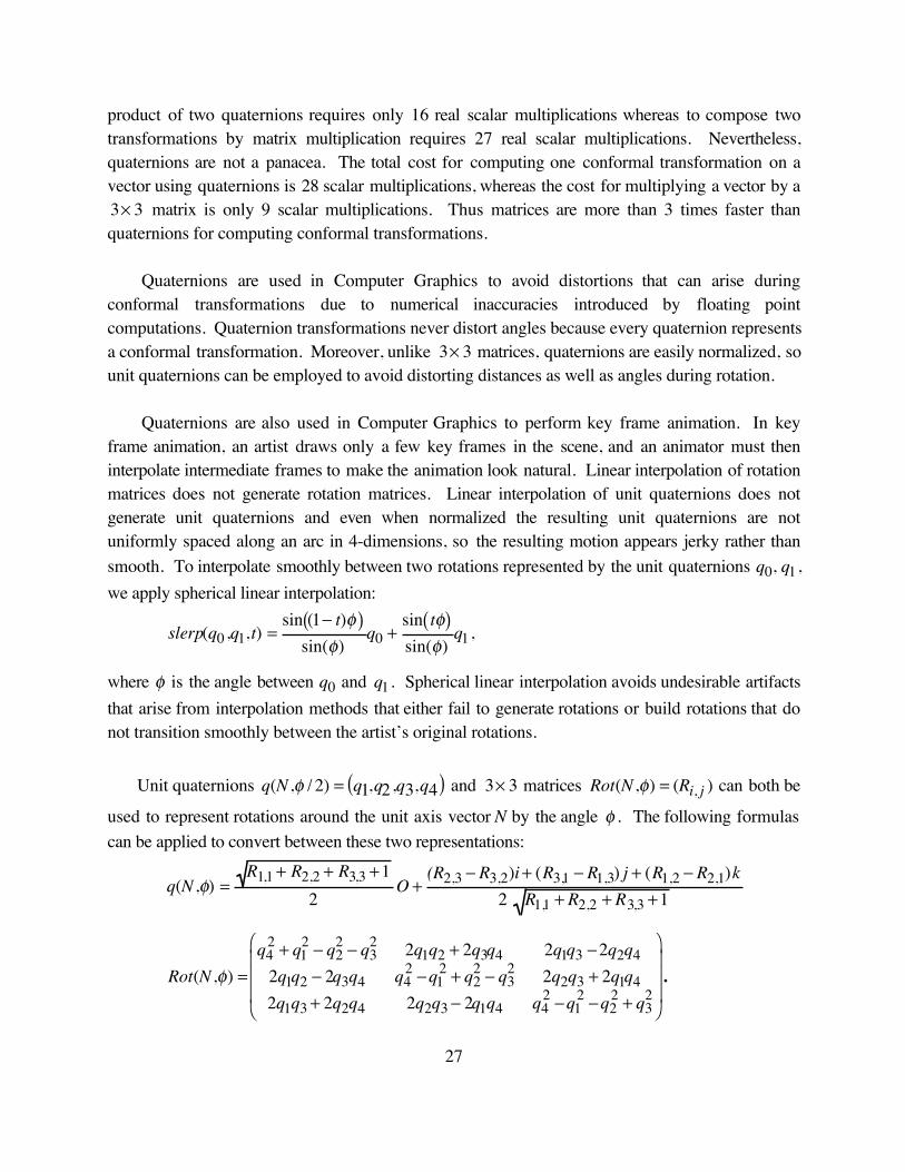
product of two quaternions requires only 16 real scalar multiplications whereas to compose two transformations by matrix multiplication requires 27 real scalar multiplications. Nevertheless, quaternions are not a panacea. The total cost for computing one conformal transformation on a vector using quaternions is 28 scalar multiplications, whereas the cost for multiplying a vector by a

�

3× 3 matrix is only 9 scalar multiplications. Thus matrices are more than 3 times faster than quaternions for computing conformal transformations.

Quaternions are used in Computer Graphics to avoid distortions that can arise during conformal transformations due to numerical inaccuracies introduced by floating point computations. Quaternion transformations never distort angles because every quaternion represents a conformal transformation. Moreover, unlike

�

3× 3 matrices, quaternions are easily normalized, so unit quaternions can be employed to avoid distorting distances as well as angles during rotation.

Quaternions are also used in Computer Graphics to perform key frame animation. In key frame animation, an artist draws only a few key frames in the scene, and an animator must then interpolate intermediate frames to make the animation look natural. Linear interpolation of rotation matrices does not generate rotation matrices. Linear interpolation of unit quaternions does not generate unit quaternions and even when normalized the resulting unit quaternions are not uniformly spaced along an arc in 4-dimensions, so the resulting motion appears jerky rather than smooth. To interpolate smoothly between two rotations represented by the unit quaternions

�

q0, q1, we apply spherical linear interpolation:

�

slerp(q0,q1,t) =sin (1− t)φ( )

sin(φ)q0 +

sin tφ( )sin(φ)

q1,

where

�

φ is the angle between

�

q0 and

�

q1. Spherical linear interpolation avoids undesirable artifacts that arise from interpolation methods that either fail to generate rotations or build rotations that do not transition smoothly between the artist’s original rotations.

Unit quaternions

�

q(N ,φ / 2) = q1,q2,q3,q4( ) and

�

3× 3 matrices

�

Rot(N ,φ) = (Ri, j ) can both be

used to represent rotations around the unit axis vector N by the angle

�

φ . The following formulas can be applied to convert between these two representations:

�

q(N ,φ) =R1,1 + R2,2 + R3,3 + 1

2O +

(R2,3 − R3,2)i + (R3,1 − R1,3) j + (R1,2 − R2,1)k2 R1,1 + R2,2 + R3,3 + 1

�

Rot(N ,φ) =q4

2 + q12 − q2

2 − q32 2q1q2 + 2q3q4 2q1q3 −2q2q4

2q1q2 − 2q3q4 q42 −q1

2 + q22 − q3

2 2q2q3 + 2q1q42q1q3 + 2q2q4 2q2q3 − 2q1q4 q4

2 −q12 −q2

2 + q32

⎛

⎝

⎜ ⎜ ⎜

⎞

⎠

⎟ ⎟ ⎟ .

27

Exercises:

1. Using Equation (2.4), verify that complex multiplication is associative, commutative, and distributes through addition.

2. Let

�

(r,θ) denote the polar coordinates of a point in the plane. Show that in polar coordinates complex multiplication is equivalent to

�

(r1,θ1) ⋅ (r2,θ2) = (r1 r2,θ1 + θ2) .

3. Here we shall derive the half angle formulas used in the text.a. Using Euler’s formula -- Equation (2.9) -- show that

�

cos(2φ) + isin(2φ) = cos(φ) + i sin(φ)( )2 .

b. Conclude from part a that:i.

�

cos(2φ) = cos2(φ) − sin2(φ) = 2cos2(φ) −1

ii.

�

sin(2φ) = 2sin(φ)cos(φ).

c. Conclude from part b that:

i.

�

cos(φ / 2) =1+ cos(φ)

2

ii.

�

sin(φ / 2) =1−cos(φ)

2.

4. Let

�

w1,w2,w be complex numbers and let

�

p(z) = anzn ++ a0 be a polynomial in the

complex variable z with real coefficients

�

a0,…,an .a. Show that:

i.

�

(w1 + w2)∗ = w1∗ + w2

∗

ii.

�

(w1w2)∗ = w1∗w2

∗

iii.

�

(wn )∗ = (w∗)n

b. Conclude from part a that if

�

p(w) = 0, then

�

p(w∗) = 0.

5. Using Equation (3.7) and the properties of dot product and cross product, verify that quaternion multiplication is associative and distributes through addition.

6. Let

�

a,b,x, y be real numbers, and let

�

z1 = a + bi ,

�

z2 = x + yi be complex numbers.a. Verify Brahmagupta’s identity:

28

�

(a2 + b2)(x 2 + y2) = (ax − by)2 + (ay + bx)2.b. Using Brahmagupta’s identity, prove that

�

| z1z2 | = | z1 | | z2 |.

7. Let

�

a,b,c, d,w,x, y, z be real numbers, and let

�

q1 = a + bi + c j + dk ,

�

q2 = w + x i + y j + zk be quaternions.

a. Verify the following generalization of Brahmagupta’s identity:

�

(a2 + b2 + c 2 + d2)(w2 + x2 + y 2 + z2) = (aw −bx − c y − dz)2 + (ax + bw + cz − d y)2

+ (ay − bz + c w + dx) 2 + (az + by −c x + dw)2.b. Using the result in part a, prove that

�

| q1q2 | = | q1 | | q2 |.

8. Consider a quaternion

�

q = q0O + q1 i + q2 j + q3 k .a. Show that

�

q = (q0O + q1i) + (q2O + q3 i) j .b. Conclude from part a that every quaternion can be represented by a pair of complex

numbers.c. Show that for any complex number α = aO + b i

jα = α∗ j .

d. Let

�

a,b,c, d be complex numbers. Using part c, show that

�

(a + b j)(c + d j) = (ac − bd∗) + (ad + bc∗) j .

9. Let q be an arbitrary quaternion. Define

�

eq = O + q +q2

2!+

q3

3!+

a. Show that if N is a unit vector, then

�

eλ N = cos(λ )O + sin(λ)N .b. Conclude from part a and Proposition 3.4 that a vector v can be rotated around a unit vector

N through the angle

�

φ by sandwiching v between

�

q = eφN /2 and

�

q∗ = e−φN /2 .

10. Consider two unit vectors

�

v0,v1. Let

�

φ be the angle between

�

v0 and

�

v1 and let

�

w =v0 × v1

| v0 × v1 |.

a. Using the results of Exercise 9, show that:

i.

�

slerp(v0,v1,t) = etφw /2 v0 e−t φ w/2

29

ii.

�

v1∗v0 = eφw

b. Conclude from part a that

�

slerp(v0,v1,t) = (v1∗v0)t /2 v0 v0

∗ v1( ) t /2.

11. In this exercise we explore the effect of sandwiching on points in affine space.a. Show that for any quaternions

�

q,a,b

�

Sq(a + b) = Sq(a) + Sq(b) .b. Show that:

i.

�

Sq(N ,θ )(O) = O

ii.

�

−SN (O) = −Oiii.

�

S c O(O) = c O

c. Conclude from parts a,b that if P is a point in affine space, theni.

�

Sq(N,φ /2)(P) rotates the point P by the angle

�

φ around the line L through the origin

parallel to the vector N.ii.

�

−SN (P) is not the mirror image of P in the plane through the origin perpendicular to the unit normal vector N, (For the correct sandwiching formula for mirror image on points, see Exercise 15.). Give a geometric interpretation of

�

−SN (P).iii.

�

S c O(P) scales the mass of P by the factor c, but leaves the location of P unchanged.

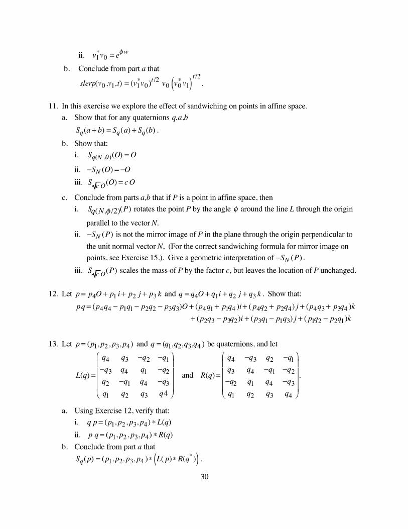
12. Let

�

p = p4O + p1 i + p2 j + p3 k and

�

q = q4O + q1i + q2 j + q3 k . Show that:

�

pq = (p4q4 − p1q1 − p2q2 − p3q3)O + (p4q1 + p1q4 )i + ( p4q2 + p2q4) j + (p4q3 + p3q4 )k + (p2q3 − p3q2)i + (p3q1 − p1q3) j + ( p1q2 − p2q1)k

13. Let

�

p = (p1, p2, p3, p4) and

�

q = (q1,q2,q3,q4 ) be quaternions, and let

�

L(q) =

q4 q3 −q2 −q1−q3 q4 q1 −q2q2 −q1 q4 −q3q1 q2 q3 q4

⎛

⎝

⎜ ⎜ ⎜ ⎜

⎞

⎠

⎟ ⎟ ⎟ ⎟

and

�

R(q) =

q4 −q3 q2 −q1q3 q4 −q1 −q2−q2 q1 q4 −q3q1 q2 q3 q4

⎛

⎝

⎜ ⎜ ⎜ ⎜

⎞

⎠

⎟ ⎟ ⎟ ⎟

.

a. Using Exercise 12, verify that:i.

�

q p = (p1, p2, p3, p4) ∗L(q)ii.

�

p q = (p1, p2, p3, p4) ∗R(q)b. Conclude from part a that

�

Sq(p) = (p1, p2, p3, p4 )∗ L( p)∗R(q∗)( ) .

30

c. By direct computation, verify that

�

L(p) ∗R(q∗) =

q42 + q1

2 − q22 − q3

2 2q1q2 + 2q3q4 2q1q3 − 2q2q4 0

2q1q2 − 2q3q4 q42 − q1

2 + q22 − q3

2 2q2q3 + 2q1q4 0

2q1q3 + 2q2q4 2q2q3 − 2q1q4 q42 − q1

2 − q22 + q3

2 0

0 0 0 q12 + q2

2 + q32 + q4

2

⎛

⎝

⎜ ⎜ ⎜ ⎜ ⎜

⎞

⎠

⎟ ⎟ ⎟ ⎟ ⎟

.d. Conclude from parts b,c that if

�

q = q(N ,φ / 2) , then

�

Rot(N ,φ) =q4

2 + q12 − q2

2 − q32 2q1q2 + 2q3q4 2q1q3 −2q2q4

2q1q2 − 2q3q4 q42 −q1

2 + q22 − q3

2 2q2q3 + 2q1q42q1q3 + 2q2q4 2q2q3 − 2q1q4 q4

2 −q12 −q2

2 + q32

⎛

⎝

⎜ ⎜ ⎜

⎞

⎠

⎟ ⎟ ⎟ .

14. Let

�

q = q4O + q1i + q2 j +q3k .a. By direct computation show that

i.

�

qi q∗ = q42 + q1

2 −q22 −q3

2, 2q1q2 + 2q3q4,2q1q3 − 2q2q4( )ii.

�

q j q∗ = 2q1q2 −2q3q4,q42 −q1

2 + q22 − q3

2,2q2q3 + 2q1q4( )iii.

�

q k q∗ = 2q1q3 + 2q2q4,2q2q3 −2q1q4,q42 −q1

2 −q22 + q3

2( )b. Conclude from part a that if

�

q = q(N ,φ / 2) , then

�

Rot(N ,φ) =q4

2 + q12 − q2

2 − q32 2q1q2 + 2q3q4 2q1q3 −2q2q4

2q1q2 − 2q3q4 q42 −q1

2 + q22 − q3

2 2q2q3 + 2q1q42q1q3 + 2q2q4 2q2q3 − 2q1q4 q4

2 −q12 −q2

2 + q32

⎛

⎝

⎜ ⎜ ⎜

⎞

⎠

⎟ ⎟ ⎟ .

15. Let L(q) and R(q) be as in Exercise 11, and let N be a unit vector.a. By direct computation, verify that

�

L(N) ∗R(N) =

1− 2N12 −2N1N2 −2N1N3 0

−2N1N2 1− 2N22 −2N2N3 0

−2N1N3 −2N2N3 1− 2N32 0

0 0 0 −1

⎛

⎝

⎜ ⎜ ⎜ ⎜ ⎜

⎞

⎠

⎟ ⎟ ⎟ ⎟ ⎟

b. Let Mir3× 3(N) be the 3× 3 matrix that mirrors vectors in the plane perpendicular to N. Using part a, show that:

31

Mir3× 3(N) =

1 − N12 −2N1N2 −2N1N3

−2N1N2 1− N22 −2N2N3

−2N1N3 −2N2N3 1− N32

⎛

⎝

⎜⎜⎜⎜

⎞

⎠

⎟⎟⎟⎟

c. Let P = (p1, p2 , p3,1) be a point in affine space and let

�

Mir4× 4(N) =Mir3× 3(N) 0

0 −1⎛ ⎝ ⎜

⎞ ⎠ ⎟ =

1− 2N12 −2N1N2 −2N1N3 0

−2N1N2 1− 2N22 −2N 2N3 0

−2N1N3 −2N2N3 1− 2N32 0

0 0 0 −1

⎛

⎝

⎜ ⎜ ⎜ ⎜

⎞

⎠

⎟ ⎟ ⎟ ⎟

..

Show that the mirror image of P in the plane through the origin perpendicular to the unit normal N is given by

(p1, p2, p3,−1)∗Mir4× 4 (N) .d. Conclude from parts a and c the mirror image of a point P in the plane through the origin

O perpendicular to the unit normal N is given by sandwiching P − 2O between two copies of N.

16. Show that:a

�

q(N ,φ)−1 = q(N ,φ)∗ = q(N,−φ) = q(−N,φ)b.

�

rot(N,φ)−1 = rot(N ,φ)T = rot(N ,− φ) = rot(−N ,φ)

17. Let v be a vector and q be a unit quaternion. Show thata.

�

S−q (v) = Sq(v) .

b. If

�

Sq(v) rotates the vector v around the unit vector N by the angle

�

θ , then

�

Sq∗(v) rotates the vector v around the unit vector N by the angle

�

−θ .

18. Let

�

v,w be unit vectors. a. Show that:

i.

�

v w is a unit quaternion.ii.

�

Sv w (w) lies in the plane of the vectors

�

v,w .

iii. v bisects the angle between w and

�

Sv w (w) .

b. Prove that mirroring a vector u in the plane perpendicular to w and then mirroring the resulting vector in the plane perpendicular to v is equivalent to rotating the vector u around the vector

�

v × w by twice the angle between w and v (see also Exercise 20).

19. In this exercise we will study the composite of two rotations.a. Show that if p and q are unit quaternions, then

�

pq is a unit quaternion.32

b. Using part a, show that

�

q(N1,φ1)q(N2,φ2) = q(N ,φ) ,wherei.

�

cos(φ / 2) = cos(φ1 / 2)cos(φ2 / 2) − sin(φ1 / 2)sin(φ2 / 2)(N1 ⋅N2)

�

ii. sin(φ / 2)N = cos(φ2 / 2)sin(φ1 / 2)N1 + cos(φ1 / 2)sin(φ2 / 2)N2 + sin(φ1 / 2)sin(φ2 / 2)N1 × N2

c. Conclude from part b that

�

q(N ,φ1)q(N,φ2) = q(N ,φ1 + φ2) .d. Using parts b,c show that

i.

�

rot(N2,φ1) ∗ rot(N1,φ2) = rot(N,φ)ii.

�

rot(N,φ1)∗ rot(N ,φ2) = rot(N,φ1 + φ2).

20. In this exercise we will show that every rotation is the composite of two reflections. Let N be a unit vector and let

�

u,v be two unit vectors in the plane perpendicular to N with

�

sgn(u,v,N) > 0 and

�

∠(u,v) = φ / 2. Show thata.

�

q(N ,φ / 2) = −v ub.

�

Sq(N,φ /2)(w) = (v u) w (uv)

c.

�

Sq(N,φ /2) = Sv Sud. Conclude from part c that every rotation is the composite of two reflections.

21. In this exercise we will develop formulas for some non-conformal affine transformations (see Chapter 12) using quaternions.

a. Show that:

i.

�

(N ⋅v)O =−(v N + N v)

2

ii.

�

N ×v =N v − v N

2b. Using the results of part a, verify that. i. Orthogonal Projection -- onto the plane perpendicular to the unit normal N

�

vnew =v − SN (v)

2ii. Parallel Projection -- onto the plane perpendicular to the unit normal N in the

direction parallel to w

�

vnew = v −v N w + N v w

w N + N w

33

iii. Non-Uniform Scaling -- along the direction w by the scale factor c

�

vnew =v − Sw (v)

2+ c

v + Sw (v)2

22. In this exercise we will show how to use sandwiching to compute perspective projection.Let 0 < θ < π , and let• S = the plane through the point O + cot(θ)N ≡ Tq( N , −θ)(N) perpendicular to the unit

normal N • E = O + cot(θ) − csc(θ)( )N = eye point (at a distance csc(θ ) from the plane S)

• P = a point in 3-dimensionsa. Let

-- v⊥ = a vector perpendicular to N

-- v = a vector parallel to N

Using Propositions 3.2 and 3.3, show that-- q(N , − θ / 2) v⊥ q(N , − θ / 2) is the identity on v⊥--

q(N , − θ / 2) v q(N , −θ / 2) rotates

v by the angle −θ in the plane of O,N

b. Using part a, show that• q(N , − θ / 2) (P − E) q(N , − θ / 2) is a mass-point, where:

-- the point is located at the perspective projection of the point P from the eye point E onto the plane S;

-- the mass is equal to d sin(θ) , where d is the distance of the point P from the plane through the eye point E perpendicular to the unit normal N.

(Hint: See Figure 10)

c. Conclude from part b that a perspective projection in 3-dimensions corresponds to a simple rotation in 4-dimensions.

d. Let q = q(N , −θ / 2) = (q1,q2,q3,q4 ) . Using part b and the definition of the matrices L(q) and R(q) in Exercise 13, show that the 4 × 4 rotation matrix corresponding to perspective projection is given by

�

Persp(N ,θ) = L(q) ∗ R(q) =

1− 2q12 −2q1q2 −2q1q3 −2q1q4

−2q1q2 1− 2q22 −2q2q3 −2q2q4

−2q1q3 −2q2q3 1− 2q32 −2q3q4

2q1q4 2q2q4 2q3q4 2q42 −1

⎛

⎝

⎜ ⎜ ⎜ ⎜ ⎜

⎞

⎠

⎟ ⎟ ⎟ ⎟ ⎟

e. Generalize the result in part b to arbitrary position of the eye point E and the plane of projection S. (Hint: Perspective projection and translation commute.)

34

�

E(eye) = O + cot(θ) − csc(θ)( )N

�

•

�

S (Perspective Plane)

�

(Perspective Point)

�

P

�

Pnew

�

Q = O + cot(θ) N

dNv

P − E

csc(θ) vd

csc(θ )N

�

•

�

•�

•R

�

•

Figure 10: By similar triangles, the point

Pnew = O + cot(θ )N + csc(θ ) vd

= E + csc(θ)N + csc(θ) vd

is the perspective projection of the point P from the eye point E onto the plane S through the point Q = O + cot(θ) N perpendicular to the unit normal N.

Programming Projects

15.1 Quaternion AlgorithmsImplement quaternion multiplication.a. Use quaternion multiplication to:

i. rotate vectors in 3-dimensions.ii. mirror vectors in 3-dimensionsiii. project points from an eye point E into a perspective plane S (see Exercise 22)

b. Compare these quaternion techniques to the corresponding matrix methods for speed and accuracy.

15.2, Key Frame AnimationGive some examples of key frame animation, using quaternions together with spherical linear interpolation (SLERP).

35