beaked whale habitat modelling report

Habitat Modelling of beaked whales in the Coral Sea (draft)

Douglas H. Cato1,2, Eleanor Bruce2, Rebecca A.Dunlop3, Daniel Harrison2, Natalie Soars2, Edwina Tanner2, Yuichiro Yasumoto2, Michelle

Blewitt2, and Iain Parnum4

Final Report to the Australian Marine Mammal Centre for project entitled Beaked whale habitat modelling part of Coral Sea using environmental data and acoustic detection survey

data (application 09/32 of 24 March 2009).

1 Defence Science and Technology Organisation, PO Box 44, Pyrmont, NSW 2009 2 University of Sydney, NSW 2009 3 University of Queensland, Qld, 4343 4 Curtin University

Habitat Modelling of Beaked Whales

EXECUTIVE SUMMARY

This document reports the results of a project “Beaked whale habitat modelling part of the Coral Sea using environmental data and acoustic detection survey data” funded by a grant from the Australian Marine Mammal Centre. The aim was to develop a habitat map of an offshore area of the Coral Sea by correlating acoustic detections of beaked whales with environmental variables such as sea floor and oceanographic properties. This was intended as a first step in development of general prediction methods for beaked whale distributions around Australia. The area has a range of habitats which include underwater topography typical of that previously associated with beaked whale habitat. Water depths vary from 300 to over 3,500 m and include the continental slope in the western part of the area and coral islands with steep sloping edges to the east. This project uses data on the acoustic detection of beaked whales in an area of the Coral Sea from two surveys of three weeks, one in August and September 2008 and the other in July 2009. The surveys and the analysis of the data to obtain the acoustic detections and beaked whale distributions were part of a separate project funded by the Australian Department of Defence. The area surveyed is used for joint exercises by the Royal Australian Navy and the U.S. Navy. The distribution of beaked whales in the area was required in order to manage impact of the exercises on the beaked whales. There have been a few occasions in the northern hemisphere of whale strandings coincident with naval exercises, and beaked whales were overrepresented in these strandings. Beaked whales are elusive and rarely seen. Their echolocation vocalisations or “clicks”, however, are sufficiently different to those of other toothed whales for them to be detected acoustically, although the differences are subtle. Hence using passive acoustic surveying for beaked whales has the potential to be useful so this method was trialled in the Coral Sea. Acoustic data were recorded during the surveys using a towed hydrophone array at around 10 m depth and two drifting acoustic recording systems (“acoustic loggers”) each with hydrophones at a depth of 400 m. This system turned out to be effective providing many detections over the area. The acoustic detection range is small enough to localise a detection to a circle of radius less than 4 km from the receiver (the array had only two closely spaced hydrophones so was of limited use in directional localisation). Just how much less depends on a number of factors and generally the detection range would be much less than 4 km. We have chosen a circle of radius 2 km around a detection position as the area of localisation. An individual beaked whale may produce large numbers of clicks over periods of up to around 40 min so the numbers of clicks detected are not indicative of the number of beaked whales. Beaked whale clicks occur in long click trains during deep foraging dives (up to 1 h duration). Large numbers of clicks are produced with inter-click separation of typically about 300 ms. Usually, if a whale is in range of detection, not all clicks would be detected because the sound is transmitted in a narrow beam and would only be detected if the beam is pointing towards the receiver. Beaked whales, however, swing the transmission beam widely as they forage, so the probability is high that some clicks would be detected if the whale is within detection range. For these reasons, the number of clicks detected is not an indication of the number of beaked whales detected. Detections of click trains tended to come in bursts separated by significant intervals, so we designated contiguous trains of click or bursts as “detections” for the purpose of the modelling. For the purpose of providing absence data for habitat modelling, we split the transects of the acoustic receivers into 30 min segments and designated the distance covered during each segment as the diameter of a circle forming a detection area. If clicks were detected during the 30 min segment, it was counted as a presence, whereas if clicks were not detected it was counted as an absence. The towed array travelled about 5.5. km in one segment, the loggers much less distance. Autocorrelation of presence/absence series for the segments showed negligible correlation between segments for the towed array but some correlation for the loggers as might be expected since they move at a much slower rate, drifting with the currents. Analysis of the acoustic data (a separately funded project) proved to be very long and tedious. The towed array data has been analysed for the 2008 cruise, but only cursory analysis has been conducted on the 2009 data. Automated methods of detection have been developed and these have been used with the logger data, and a separately funded project is about to commence and will apply these automated methods to the 2009 array data.


A wide range of environmental data were obtained from various sources, including remotely sensed satellite data, merged bathymetry datasets, output from numerical ocean circulation models, and parameters derived from these original data sources. Three different approaches to modelling were used:

• Histograms of detections for each environmental variable for all acoustic data sets

• A Generalised Linear Model (GLM) using presence and absences on the 2008 array data only.

• A maximum entropy model (Maxent) using the detections from the 2008 array data to train the

model and the 2009 array data to test the model. The histogram is based only on detection data and so is biased to the extent that the survey paths are not representative of the area in terms of the environmental variables used. The GLM used presence and absence information. The Maxent model uses the detections and compared the distribution of environmental variables with the distribution of these variables across an area selected to encompass the area of interest. In spite of the differences between models in terms of the approach and potential biases, there is a consistency in the results. When taken in the context of the surveys and the data collection, these indicate that the following factors are indicative of beaked whale habitat preference:

• Steep slopes in deep water, particularly near underwater canyons, reefs and continental slopes. These are indicated by the variables depth (with the qualification discussed above), steeper sea floor slopes or gradients typical of continental slopes or steep sided oceanic islands, short distances to 1000 m depth contour, and short distances to canyons.

• Cooler sea surface temperature (within the range of the data of 21° - 24°C). Since there was

significant eddying of currents in the area during the surveys, this may indicate a preference for the cold areas pinched off between warm core eddies evident in the area. Such cold areas have been shown to be more biological productive than the surrounding water.

• More saline water.

Although the GLM found that chlorophyll-a (from satellite) was a significant factor, the conclusions that can be drawn are limited because of the many of the chlorophyll-a records were unusable because of cloud cover. The results should allow us to make some predictions of likely beaked whale presence in other areas. This might be expected to be most effective when applied to areas where the range of values of the environmental variables are similar to those of the survey area. Further work on habitat modelling using the survey data is being conducted, using funding from other sources. When the full analysis of the 2009 array data is completed, the models will be run again to include these data. More analysis of the way potential biases in the survey method and analysis affects the results will be conducted.


CONTENTS EXECUTIVE SUMMARY ........................................................................................................................2 1. Introduction ........................................................................................................................................5

1.1 background....................................................................................................................................5 1.2. beaked whales.............................................................................................................................6 1.3. impacts on beaked whales and the need for management ........................................................7 1.4. The surveys .................................................................................................................................8 1.5 known beaked whale habitat .......................................................................................................8

2. METHODS ........................................................................................................................................9 2.1 Beaked whale detection survey data and analysis ......................................................................9

2.1.1 Details of the surveys .............................................................................................................9 2.1.2 Acoustic Analysis ................................................................................................................10 2.1.3 Acoustic detection results ....................................................................................................13

2.2. HABITAT PREFERENCE MODELLING ...................................................................................17 2.2.1. Environmental Analysis System / the Pelagic Habitat Analysis Module..............................17 2.2.2 ESRI Arc GIS......................................................................................................................17 2.2.3 Habitat models .....................................................................................................................18 2.2.4 Compiled Datasets................................................................................................................18

2.3 Data sources AND PREPARATION ..............................................................................................20 2.3.1 Environmental datasets ........................................................................................................20 BLUElink circulation model data: currents, sst, sea surface height, salinity..................................24 Satellite derived datasets: Chlorophyll-a .......................................................................................27

3. Results ..............................................................................................................................................29 3.1 detections ....................................................................................................................................29 3.2 Generalised linear model of presence/Absence .........................................................................31

3.2.1. Data exploration..................................................................................................................32 3.2.2. Model selection and comparison ........................................................................................34 3.2.3. Model Interpretation............................................................................................................37 3.2.4. Summary of findings ...........................................................................................................37

3.3 application of MaxEnt for predicting beaked whale presence....................................................39 3.3.1 Background...........................................................................................................................39 3.3.2. Model outputs ......................................................................................................................40 3.3.3. Evaluating model performance...........................................................................................41 3.3.4. Analysis of environmental variable contributions to the model...........................................43

4. Comparison of results and conclusions ...........................................................................................46 Compliance with the requirement of the project ................................................................................48 Further work ......................................................................................................................................49

REFERENCES......................................................................................................................................50


1. INTRODUCTION 1.1 BACKGROUND This document reports the results of a project “Beaked whale habitat modelling part of the Coral Sea using environmental data and acoustic detection survey data” funded by a grant from the Australian Marine Mammal Centre (AMMC). The aim of this project was to develop a habitat map of an offshore area of the Coral Sea by correlating acoustic detections of beaked whales with environmental variables such as sea floor and oceanographic properties. This would be a first step in development of general prediction methods for their distributions. The project makes use of acoustic detection data and the resulting beaked whale distributions from surveys of beaked whales which were obtained from a separate project led by DSTO and involving the Universities of Sydney, Queensland, Curtin and Macquarie Universities. This involved the execution and analysis of two acoustic surveys for beaked whales in the area and was funded by the Australian Department of Defence. There was a delay of more than a year in the commencement of the project from the notification by AMMC in November 2009 that the grant was successful. The agreement between AMMC and the University of Sydney covering the project was not signed until 14 May 2010. There were further delays until an agreement was reached between the University of Sydney and the Defence Science and Technology Organisation (DSTO). This was signed in November 2010, and funding did not flow until early 2011. Two combined acoustic and visual surveys of beaked whales were conducted in the Coral Sea north east of Fraser Island off the east coast of Australia in the area of the Cato Trough. The surveys were of approximately three weeks duration, one in August and September 2008 and the other in July 2009. They covered a rectangular area extending about 171 km E-W and 60 km N-S (Fig. 1.1) with boundaries to north and south of 22°20´ S and 23°20´ S respectively, and to west and east 154°00´ E and 155°40´ E respectively (centred about 230 km NW of N tip of Fraser Is). Water depths varied from 300 to over 3,500 m and included the continental slope in the western part of the area and coral islands with steep sloping edges to the east. Beaked whales are known to prefer deep water and steep slopes (Macleod & D’Amico, 2006). Naval exercises (known as Talisman Saber) involving both the Royal Australian Navy and the U.S. Navy are conducted every two years in the area. The purpose of the surveys was to obtain information about the distribution of beaked whales over the area as part of the mitigation measures taken to avoid adverse impact on the whales. There have been several strandings of whales with a predominance of beaked whales species in the northern hemisphere associated with naval exercises.


Figure 1.1. Map showing the location of the survey area and the bathymetry. Water depth varies from 300 m to over 3,500 m. The northern and southern boundaries are at latitudes 22°20´ S and 23°20´ S respectively, and the western and eastern boundaries at 154°00´ E and 155°40´ E respectively. Fraser Is. is evident to the south west of the area.

1.2. BEAKED WHALES Beaked whales (family Ziphiidae) are small to medium sized toothed whales (suborder: Odontoceti) ranging in length between species from about 3.5 to 13 m. They generally inhabit deep waters offshore and are very elusive and rarely sighted. Consequently, little is known about their biology and distributions, apart from what has been learnt from occasional stranded animals and rare sightings. Twelve species have been recorded in the Australian stranding records collected by state authorities and compiled by Environment Australia (now the Department of Sustainability, Environment, Water, Population and Communities – SEWPaC). What is known about beaked whale habitat preference indicates that they forage in deep water near the continental slope or steep sided islands. Currents in the survey region show large scale eddies. Forecasts by the Australian Government ocean forecasting system BLUElink showed significant eddies with cold core intrusions in the area during the surveys (http://www.bom.gov.au/oceanography/forecasts/). The deep water, steep slopes and cold core eddy intrusions suggest that the area includes the type of habitat preferred by beaked whales. Significant advances in knowledge of beaked whales have resulted from attaching DTAGs to the whales. DTAGs (Johnson & Tyack, 2003) are attached by suction caps and are timed to release after a selected period, typically several hours. A DTAG records the sound received by the whale as well as the whale’s three dimensional motion (using accelerometers). Thus a three dimensional map can be developed of the movements of the whale over the period of attachment. The first application to beaked whales (Johnson et al., 2004) was to two Cuvier’s beaked whales (Ziphius cavirostris) in the Ligurian Sea (part of the Mediterranean Sea) and to two Blainville’s beaked whales (Mesoplodon densirostris) near the Canary Islands.


These results and those of other studies with DTAGs (Madsen, et al., 2005; Johnson et al., 2006; and Tyack et al., 2006) have shown that the beaked whales make foraging dives for periods of about 1 h at depths up to 1800 m or more, producing series of echolocation clicks when deeper than 200 m. Recently, recordings of Gervais’ beaked whales (Mesoplodon europaeus) have been published (Gillespie et al., 2009) and their vocalizations are generally similar to those of the other two species discussed above. The DTAG data provided the first samples of echolocation vocalisations from beaked whales. Toothed whales in general produce short, intense pulses of clicks of a few cycles covering a broad frequency band. An echolocation function has been established for many species and is assumed for other species. Click characteristic range in duration from order of tens of microseconds (some dolphins: Au 1993) to order milliseconds (sperm whales: Backus & Schevill, 1966; Madsen et al, 2002) and frequency bands from around 1 kHz - 230 kHz for sperm whales to 20 - 160 kHz for some dolphins. The recorded beaked whale clicks are subtly different to the general characteristics of toothed whale clicks having pulses with typically 7 – 10 cycles which swept in frequency from about 25 kHz to more than 50 kHz over the duration (Johnson et al., 2004). The frequency band lies within the broad range for all toothed whales but is distinctive, as is the frequency sweep. With these characteristics, it is possible to distinguish beaked whales from other toothed whales in acoustic recordings at sea.

1.3. IMPACTS ON BEAKED WHALES AND THE NEED FOR MANAGEMENT Beaked whales have been predominant in several incidents of whale strandings that have occurred at similar times and in the general area of a few naval exercises in the Northern Hemisphere. The tactical sonar used in the exercises has been claimed by many to be the cause of the strandings, the actual cause is not known (Tyack et al., 2011). Several theories of ways in which sonar may cause whales to strand have been produced but have lacked supporting evidence. For example, an interim report on strandings on islands of the Bahamas in 2000 at the time of naval exercises in the area attributed the cause to the mid frequency naval sonar (Evans and England, 2001). They did not, however, produce evidence that sound waves could produce the trauma observed and such evidence does not appear to be available. Generally, it has not been possible to determine where the beaked whales were relative to the ships prior to the strandings, but the spatial extent of strandings suggests that the whales may have been at significant distances from the ships where received levels would have been relatively low, suggesting that the effect is most likely to be a behavioural response. The areas where the strandings associated with naval exercises occurred are generally areas close to deep water typical of beaked whale habitat, particularly with steep sided islands. More recent studies have shown that beaked whales flee from naval exercises and playback of various sounds. Studies of the movements of Blainville’s beaked whales (Mesoplodon densirostris) in the U.S. Navy Atlantic Undersea Test and Evaluation Center (AUTEC), in the Tongue of the Ocean near Andros Island in the Bahamas, have shown that the whales moved away from naval exercises when conducted in the area and then returned in the two to three days after the exercises (Boyd et al., 2007; Tyack et al. 2011). Experiments in the same area in which beaked whales fitted with DTAGs were exposed to playback of sonar, pseudorandom noise and sounds of killer whales (Orcinus orca) found that the whales showed evasive response when received sound levels reached about 140 dB re 1 µPa for the sonar and noise playback but at much lower levels for the killer whale sounds (98 dB re 1 µPa). These levels are well below those typical of criteria accepted for whale exposure to anthropogenic noise in environmental regulations (such as the Australian seismic guidelines and background paper: EPBC Act Policy Statement 2.1, 2008). The relatively similar responses to playback of sonar and noise suggest that the whales may respond to any anthropogenic sounds, not just to sonar. Behavioural reactions are more likely to be due to the way the whales interpret the nature of the source rather than to specific acoustic characteristics of the sound as such, apart from the way these characteristics imply a particular sound. For example, the response to playback of killer whale sounds at much lower levels than those of sonar or noise playback is consistent with the response that might be expected when predators are detected and killer whales are predators of beaked whales. The characteristics of the sounds that mattered in this case were probably those that allowed the beaked whales to recognised the source as killer whales, rather than the received level of the sounds. The above study also investigated the responses of false killer whales and pilot whales to the playback and found these to be far less pronounced than those of the beaked whales.


From these studies, the most likely explanation of the strandings attributed to naval exercises is that the whales run aground as they flee from the ships. A consistent feature of the locations of the strandings is that deep water is very close to shore, such as steep sided islands. Beaked whales appear to show much more pronounced response than the other odontocetes studied consistent with the known elusiveness of beaked whales compared with other whales. As a consequence, since the strandings, navies have adopted mitigation measures that have generally involved avoidance of areas close to steep sided shore lines close to deep water. There have been no mass strandings associated with naval exercises since 2002.

1.4. THE SURVEYS The beaked whale surveys in the Coral Sea included both visual observations and acoustic recordings. Generally, the effectiveness of visual surveying for beaked whales is too limited to be useful because they are so difficult to detect visually. The acoustic component of the survey was based on the assumption that sounds of beaked whales in the area would be similar enough to those recorded in the northern hemisphere. This turned out to be the case: the recorded clicks were remarkably similar to those published. The Australian stranding records showed evidence of four species in the general area: Ziphius cavirostris (Cuvier’s beaked whale), Mesoplodon densirostris (Blainville’s beaked whale), Mesoplodon layardii (Strap toothed beaked whale) and Indopacetus pacificus (Longman’s beaked whale). The first two were those with published DTAG recordings from the northern hemisphere. There are few published examples of acoustic surveys for beaked whales of the scale conducted in the Coral Sea. It was not at all clear in advance that these surveys would be successful. Nor was the scale of the analysis clear at the time. It turned out that the acoustics surveys were quite successful in detecting beaked whales, but the analysis of the data has proved to be long and time consuming. This is partly due to the large amount of data collected and partly due to the complexity of separating sounds of beaked whales from the large number of generally similar sounds recorded from other species of toothed whales during the surveys. Full manual analysis has been completed for the towed array from the 2008 cruise but only a cursory analysis has been completed for the 2009 cruise. Automated detection methods have been developed and used for the logger data and is in progress for the 2009 array data as part of another project (funded separately). All available data are used for the habitat modeling project.

1.5 KNOWN BEAKED WHALE HABITAT In addition to the information discussed above about the dive profiles of beaked whales, several papers provide information about the environmental properties where beaked whales are found. Waring et al (2001) reported that beaked whales were found in waters on the continental shelf edge and continental slope, and waters cooler (22.3° ± 0.5°C) than those where sperm whales were found. MacLeod and Zur (2005) found beaked whales had a preference of sea floor slopes of 3.8°-16.5° to the horizontal. Aspect of slope and water depth were also important indicators. D’Amico et al (2003) found an association between beaked whales presence correlated with cooler water with higher chlorophyll production. Cuvier’s beaked whale showed a preference for submarine canyons where there is a frontal interface. Ferguson et al. (2006) found beaked whales in deeper waters than found in other studies: 700 - 3,500 m. Gannier and Epinat (2008) and Moulins et al. (2007) found generally similar results to the above studies.


2. METHODS 2.1 BEAKED WHALE DETECtION SURVEY DATA AND ANALYSIS Although the surveys and analysis of the data were conducted as part of another project (funded separately), the nature and limitations of the survey and the methods of detection, however, need to be considered in some detail, since they affect the habitat modelling.

2.1.1 Details of the surveys Two surveys were conducted in the Coral Sea off the east coast of Australia of about three weeks duration: A three week survey was conducted in August, September 2008 and another in July 2009. The surveys covered a box extending about 171 km E-W and 60 km N-S (Fig. 1), the coordinates of the NW corner of the box being 22°20´ S and 54°00´ E. Water depths varied from 300 to over 3,500 m and included the continental slope in the western part of the area and coral islands with steep sloping edges to the east. A Royal Australian Navy landing craft, HMAS Labuan was provided for the surveys which involved both visual and acoustic monitoring. Two types of acoustic passive recording systems were used: a towed array and two drifting recording systems (“acoustic loggers”). The towed array supplied by Ecologic UK Ltd., consisted of two mid frequency channels (500 Hz – 30 kHz) and two high frequency channels (500 Hz – 150 kHz) and depth sensor. The hydrophones were closely spaced at the end of the 400 m cable. Data were recorded on hard disk via a data acquisition card sampling at 300 kHz (giving an upper frequency limit of 150 kHz) in files of 30 min duration. The two drifting systems (“acoustic loggers”) were developed by the Centre for Marine Science and Technology at Curtin University for the purpose and comprised a computer controlled recording system in a container suspended below surface buoys and with a hydrophone at a depth of 400 m. A suspension system was used to minimize transfer of surface motion to the hydrophone. A radio beacon transmitted the GPS position of the buoys allowing the survey team on the ship to keep track of their position. The logger systems were deployed for a period of a few days at a time, and then recovered, the data downloaded and the systems redeployed. While the towed array provided continuous monitoring, the much deeper hydrophones of the drifting systems were considered to provide an advantage in the detection of clicks from beaked whales foraging at depth. The data were sampled at 192 kHz (giving and upper frequency limit of 96 kHz) and recorded onto a Sound Devices type 722 digital recorder, with 300 s of recording made every 900 s. There were 210 h of visual survey in 2008 and 200 h in 2009, with two observers throughout. More than 700 individual whales from about 12 species (a small number of individuals were not identified to species), mainly toothed whales from dolphins to sperm whales were seen. There were six sightings of 12 individual beaked whales in 2008, possibly Cuvier’s based on colouring, and only one sighting in 2009 (possibly Longman’s). The towed array provided 185 h of recording in 2008 and a similar amount in 2009. The drifting acoustic loggers provided 130 h in 2008 and 95 in 2009. The drifting systems were first used on these surveys and proved quite successful. They moved between 30 and 50 km over the few days of each deployment and remained within radio detection range throughout.

Coverage of area The ship HMAS Labuan towed the towed array at a speed of nominally 6 knots (about 11 km/h). Nominal transects for the ship to follow while towing the array were designed to cover the area. However, these were modified by a number of factors. Firstly, the ship deployed and recovered the two drifting loggers at intervals of two to three days so that the ship had to divert from the nominal transects to wherever the loggers were at the time of recovery, then return to the transects. The array continued to operate during this deviation from the nominal transects, except while the ship manoeuvred to recover and redeploy the loggers, when the array had to be recovered to avoid fouling the propellers. Secondly, limitations on the sea keeping ability of LABUAN while towing the array meant that it was necessary to alter the course in higher sea states depending on the direction of the sea relative to the course. In some bad weather conditions, LABUAN had to shelter behind one of the islands. Thirdly, because current knowledge of beaked whale habitat preferences indicated that they


preferred deep water, generally deeper than a few hundred metres, it was desirable to cover the deeper water initially in case the full area could not be covered in the time available. An attempt was made in the design of the second cruise to balance this bias towards deeper water that occurred in the first cruise. These constraints resulted in transects that were irregular but do appear to provide reasonable coverage of most of the area, with somewhat less coverage of the shallow water on the western side of the area. The paths taken by the loggers depended on the drag caused by the currents over the 400 m depth range of the line supporting the hydrophone. This could not be predicted in advance since no forecast of the currents at depth were available.

2.1.2 Acoustic Analysis The main method of detecting the presence of beaked whales was from analysis of the acoustic recordings taken during the cruises. This is a tedious and lengthy process. Beaked whale clicks are typically about 400 µs in duration, so that one click is about one part in 1.7 x 109 of the duration of the 185 h of data for the towed array from the 2008 cruise. Data were analysed using Adobe Audition (Adobe Systems). Manual detection of clicks required searching through spectrograms of small sections of the data to find energy that covered the right frequency range, then zooming in further and checking the characteristics of the waveform (an upsweep in frequency indicated by progressive reduction in the period of successive cycles, with the correct duration over the click). The data had to be divided into sufficiently short time intervals for the beaked whale clicks to be visually detectable (the frequencies are outside the range of hearing, so aural detection was not effective). Sections of the recording with beaked whale click trains were then saved as separate files and further measurements taken (start frequency, end frequency, peak frequency, click train duration, inter-click-interval). The analysis was further complicated by the large number of detections of clicks from many other species of toothed whales that were recorded during the cruises. Although beaked whale clicks differ sufficiently in acoustical characteristics from those of other odnotocetes to allow their clicks to be identified with a high degree of confidence, the differences are subtle. Confirmation that a click is from a beaked whale requires detailed characteristics of each click to be examined. The acoustic analysis involved months of work for the 2008 array data alone. A cursory analysis of a few weeks was conducted on the 2009 array data which provided some detections but is by no means complete. The 2009 array data are, however, included in this analysis. It was apparent from the start that an automated method of detection was needed in order to complete the analysis in a reasonable time scale. Automated detection is far more difficult in the presence of clicks from other odontocete species than it would be without them, because of the similarities in characteristics of clicks across toothed whale species. A method has been developed (Parnum et al., 2011), again as part of another project and funded separately. Checking the detections by the automated methods against the manual detections is in progress as part of this other project. It is time consuming and dependent on funding and so far it has been confined to a subsample of detections from the towed array in 2008. Preliminary results suggest that detections by the automated method are matched by the manual method, but a small proportion of the manual detections are missed by the automated analysis. Further work is required to develop detection performance statistics for the automated method. Since beaked whales click for long periods during a dive, detection of only a small proportion of these clicks is sufficient to establish the presence of the whale. Hence we can tolerate missing some proportion of detections for the purpose of the habitat study, and the failure to detect a small proportion of the clicks is probably not a problem in establishing absences of beaked whales. We therefore have acoustic detection data of beaked whales for the towed array in 2008 from manual and automated methods, a limited amount for 2009 from cursory manual analysis, and automated analysis of the logger data for 2008 and 2009. Automated analysis of the 2009 array data is expected to be completed in April 2012 and the habitat modelling described in this report will be rerun using all the data.


Establishment of beaked whale presence. For the purpose of the habitat modelling, we need to establish criteria for establishing presence of beaked whales from the acoustic data and the spatial resolution of the detected presence. The following describes the rationale for this. It turns out that while the detection of clicks is a reliable indication of the presence of beaked whales, the number of clicks detected is of very limited use and not a reliable indication of the number of whales present. Hence we are limited to establishing presence of beaked whales without useful information on the number of whales present. Experiments with DTAGs attached to beaked whales (Johnson et al., 2004; Madsen, et al., 2005; Johnson et al., 2006; and Tyack et al., 2006) have shown that the whales make foraging dives for periods of about 1 h at depths to 1800 m or more, producing echolocation clicks when deeper than 200 m. Clicks are produced as a series for up to about 40 min, with typical click separation of about 300 ms. Click separation reduces rapidly as a whale homes in on prey. Hence large numbers of clicks may be detected for one individual. Establishing if there is more than one individual is difficult. The click separation is generally fairly consistent so it would be possible to detect two click trains if they coincided but are offset in time within the 300 ms click separation, and this would indicate that two individuals are detected. This has not been observed in the data so far. Hence we have taken the detection of clicks over a period of up to 40 min to be no more than one individual. Although beaked whale sounds have relatively high source levels, acoustic detection ranges of beaked whale clicks are limited because of the higher absorption of sound at the high frequencies of the vocalizations, and because of their narrow beam pattern. Zimmer et al. (2008) estimate that the range for 50% probability of detection using a receiver depth of 100 m would be between 1.5 and 3.8 km, and detection beyond 4 km would be very unlikely. These estimates are for low background noise and shorter ranges are to be expected for higher noise levels as conditions (e.g. wind speed) changes. Other environmental factors can affect the propagation of sound, so there will be significant uncertainty in the range of detection at any time. DTAG recordings have shown that while beaked whales change their orientation frequently as they move in search of prey, the variation of beam directions is highest horizontally and lowest vertically. This suggests that detection would be more likely with deep receivers (at depths approaching those of the whales while vocalizing) than with shallow ones, because a whale would need to point the beam towards the surface to be detected on a shallow receiver. The expectation, therefore, is that a beaked whale clicking for 40 min during a dive may be detected intermittently on the shallow hydrophones of the towed array (assuming that the whale remains in detection range). Hence gaps in click detection may not mean that the whale has stopped clicking and a new series of clicks following a gap may be from the same individual. Since there are a large number of clicks produced during a dive, the probability of detecting at least some of the clicks during a dive is likely to be much higher than the average probability of detecting one click. It is clear from Zimmer et al. (2008) that it would be very unlikely to detect a whale over the period of a dive if it is 4 km or more from the hydrophone. It is also necessary to localise the position of the detections for habitat modelling. Usually, to do this for acoustic detection would require acoustic localisation using multi-element hydrophone arrays. Such arrays are expensive and were not available for the survey cruises. There were two high frequency hydrophones on the towed array but these were too close together to be useful in localizing the source of sounds. However, because of the short acoustic detection range, a detection would be localized to a small area compared to the size of the survey area. Hence the position of the vocalizing whale could be determined with sufficient accuracy for the purpose, without attempting to use acoustic localization such as with a line array. From the modelling by Zimmer et al. (2008), and consideration of the propagation loss at the site and the detections process, we consider that it would be reasonable to assume that a detection of a click would localise the vocalising whale to within a radius of less than 4 km. This is the “slant range,” i.e. the actual distance to the whale in three dimensions, not the horizontal distance. For the towed array, the horizontal distance would typically be less than this, because of the depth of the whale. Hence the actual position of a vocalising whale in the horizontal plane may be anywhere from a few hundred metres to up to four kilometres, but would generally be significantly less than 4 km. For the purpose of habitat modelling, even 4 km localises the whale to an area that is small enough compared to the spatial scales of the environmental data. We have chosen to draw a circle of 2 km around each click detection position as a more realistic indication of the possible location of the source.


Establishment of absence of beaked whales Many ecological habitat models require absence as well as presence data in order to discern when the organism being modelled is exhibiting preference for a certain habitat characteristic rather than indifferently using the habitat available. In a survey of this kind, the absence of click detection does not mean that there were no whales within detection range of the array, or that the location is unsuitable habitat. A whale may not be actively eco-locating at the time. It may be producing eco-location ‘clicks’ directed away from the listening array, although an individual produces clicks for long periods while changing its orientation, so that there is a very high probability that it will be detected for a least some of the time that it is within range. There may be no whales within range, but it may still be suitable habitat – for example, the whales may have moved on from this area to the next possibly following movements of prey. For the purpose of obtaining absence data for habitat modelling, we have split the tracks of the hydrophones into segments equalling the distance covered in 30 min. If clicks are detected within a segment, that counts as a presence within the segment. If no clicks are detected, that counts as an absence. In 30 min, the towed array would have travelled about 5.5. km (at 11 km/h), the logger a much smaller distance. The detection of clicks within this area could not be attributed to more than one individual for the reasons discussed above but estimation of the number of individuals is not needed to establish presence. This choice is somewhat arbitrary and convenient but also considers the likely detection distance and duration of detections from an individual. There is no simple way of selecting the length or duration of a segment. Whatever the length of a segment, clicks could be detected up to almost 4 km from either end of a segment when the hydrophone is near the ends. Inspection of the array data for 2008, showed that if clicks occurring within a period of 40 min are grouped, the separation in time between groups of clicks varies from 71 min to many hours. The ship would cover a distance of about 13.5 km in 71 min, and clicks detected in groups separated by that distance could not have been from the same individual. The period of click groups ranges from less than 1 to 39 min, with mean of 14.4 and median of 10.5 min. Redefining click groups as a period of 20 min, gives one additional separation of 43 min in addition to those obtained with 40 min groups. The ship would travel 8.2 km in 43 min. Again it is very unlikely that two groups of clicks separated by 8.2 km of ship transect would be from the same individual. It is therefore apparent, that using segments of 30 min would lead to a reliable estimate of the number of presence locations with the array. It may, however, lead to an overestimate in the number of absences. The drifting loggers covered distances of up to 50 km during deployments which lasted up to 3 days. The average speed of the drifters was approximately 0.17 m/s. At that average speed, a logger would drift about 300 m in 30 min of a segment. This is a relatively small distance compared to the 4 km limit of the range of detection. Hence using the 30 min segment criterion, the loggers would provide a number of samples of presence or absence at each location, and there may be correlation between segments. The ship’s track was derived from the onboard GPS and subset according to the deployment record of the towed array to yield the track and times of array sampling. The sampling record for each year was then sub divided into 30 minute segments and the GPS co-ordinates of the start, middle, and end of each 30 minute segment were extracted from the GPS log. Each segment was then assigned a binomial flag to indicate presence or absence based on whether any beaked whale detections were made during that portion of the transect. Subsequent testing for conditional independence of the detection data confirmed that 30 minutes was an appropriate segment length. GPS data of ship’s track The ship’s GPS position was recorded as raw output from the GPS unit every one second to a series of text files each of a nominal 30 minute duration and matching the times of the acoustic data files. The GPS data were stored with the date in AEST time and the time in UTC time, co-ordinates were in an unusual ascii text format as such a significant amount of pre-processing to extract usable time and latitude / longitude was required. The statistical programming package “R” (R Develpment Core Team, 2005) was used to read all files into an array and perform the pre-processing steps required.


The actual time of each towed array detection was then determined by adding the time within the file at which a click train occurred to the start time and date of the file. The date and time of the detection were then cross referenced with the GPS data to obtain the position of the ship. The difference between the position of the ship and the position of the towed array was small compared to the detection range of up to 4 km discussed above, so the position of the ship was used as the centre of the detection location.

2.1.3 Acoustic detection results

Towed Hydrophone Array Detection data from the towed hydrophone array was generated by manual inspection of waveforms of the sound recordings. This process was extremely tedious and approximately 400 hours were spent analysing the recordings from 2008 alone. Only a cursory analysis has been completed for the towed hydrophone array for the 2009 survey (made aboard the vessel while at sea during the voyage). Eight beaked whale detections were identified in this analysis compared with 212 for 2008 despite a similar number of hours recorded. An identified detection within the dataset indicates that one or more ‘clicks’ were recorded and attributed to beaked whales. The number of ‘clicks’ per detection varied between 1 and 73 for the towed arrays. The echolocation clicks of a beaked whale exhibit pronounced directionality (Johnson et al., 2004) thus the number of clicks recorded is primarily a function of the location of the sensor relative to the direction in which the click was directed. As such the number of clicks per detection is not assumed to be a reliable indication of how many clicks the whale was producing nor of the number of whales clicking. This may be especially true for the towed array hydrophone which were at a depth of approximately 10 m and as such was less likely to detect clicks from foraging at depth compared with the drifting data loggers. The 2008 array detection dataset included the date and time of the start / end of detection, number of clicks in the click train, a quality estimate between 1 and 5 (1 = best quality), the range of click quality, minimum / maximum / average frequency of the waveform, and an identifier for the recording file from which it was detected. The 2009 detections included the date, time and location of each detection, and an estimate of the number of clicks, but little ancillary information. Clicks were also graded according to the certainty that they are beaked whale clicks (1 = unsure, 3 = very sure) and the SNR (1 = poor, 3 = excellent). There were significantly more detections from the recordings of the 2008 towed array then the 2009 towed array n = 212 in 2008 compared with n = 8 in 2009. The mean number of clicks per detection was similar in both years, 9.96 in 2008 and 13.50 in 2009. The cleaveland dotplot (figure 2.1) for the number of clicks per detection in 2008 indicates that there are no obvious outliers in the data. The 2009 data include far fewer detections which are likely due to the different analysis methods employed to identify detections. Although there appear to be outliers in the 2009 data when considered alone, they fall within the range of click numbers during 2008. For this reason and because there are few measurements in 2009 no measurements are rejected as outliers. For the reasons described above the number of clicks per detection are not used in the modelling of the habitat study. The detection data are treated as detection of presence only.


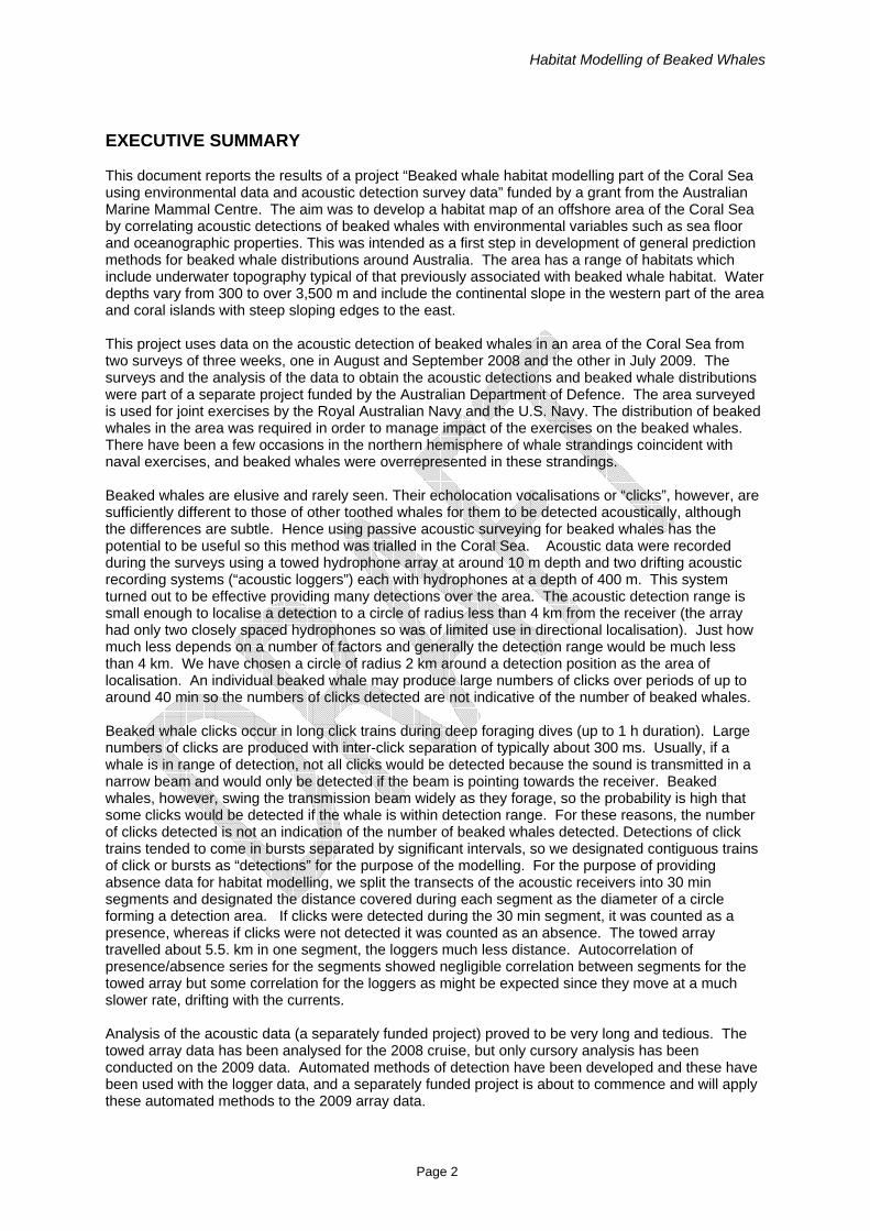
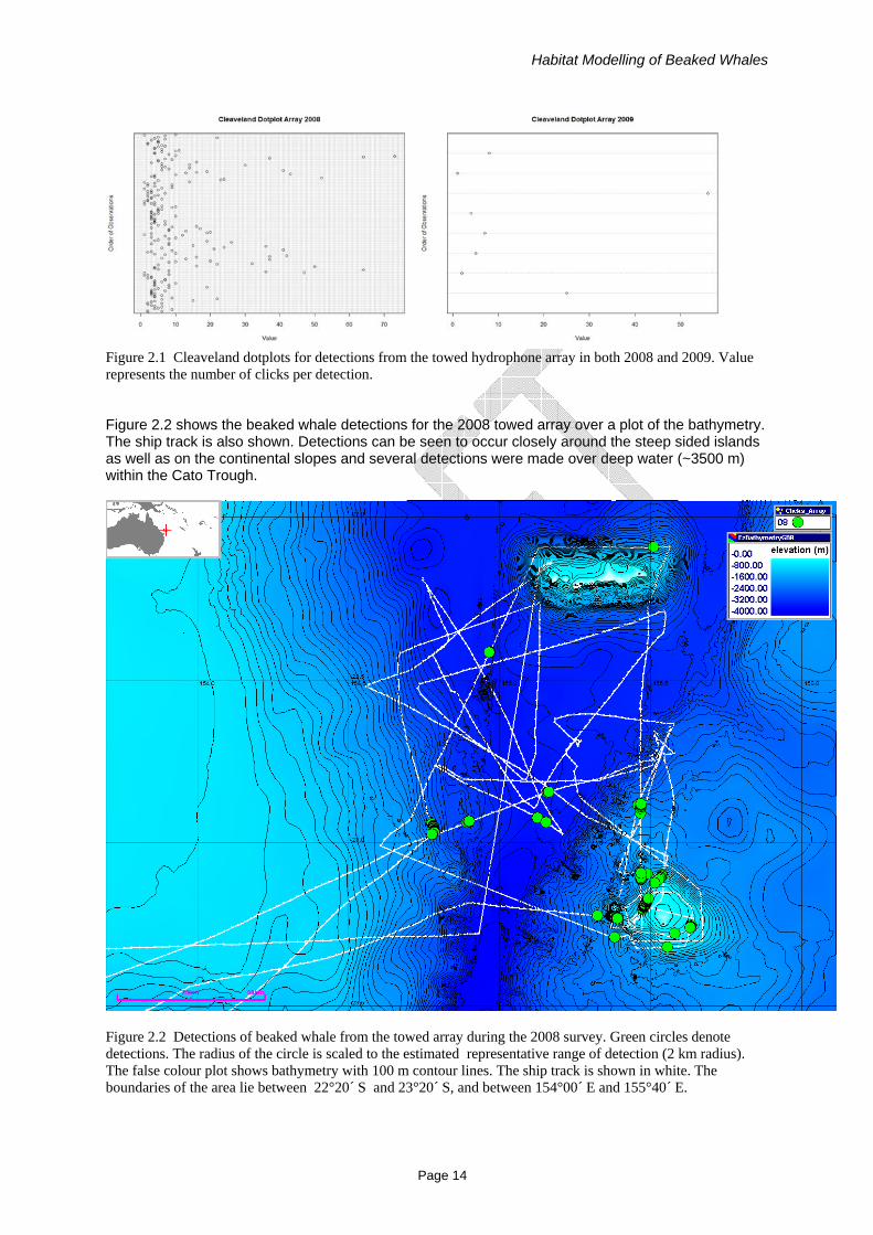
Figure 2.1 Cleaveland dotplots for detections from the towed hydrophone array in both 2008 and 2009. Value represents the number of clicks per detection. Figure 2.2 shows the beaked whale detections for the 2008 towed array over a plot of the bathymetry. The ship track is also shown. Detections can be seen to occur closely around the steep sided islands as well as on the continental slopes and several detections were made over deep water (~3500 m) within the Cato Trough.

Figure 2.2 Detections of beaked whale from the towed array during the 2008 survey. Green circles denote detections. The radius of the circle is scaled to the estimated representative range of detection (2 km radius). The false colour plot shows bathymetry with 100 m contour lines. The ship track is shown in white. The boundaries of the area lie between 22°20´ S and 23°20´ S, and between 154°00´ E and 155°40´ E.


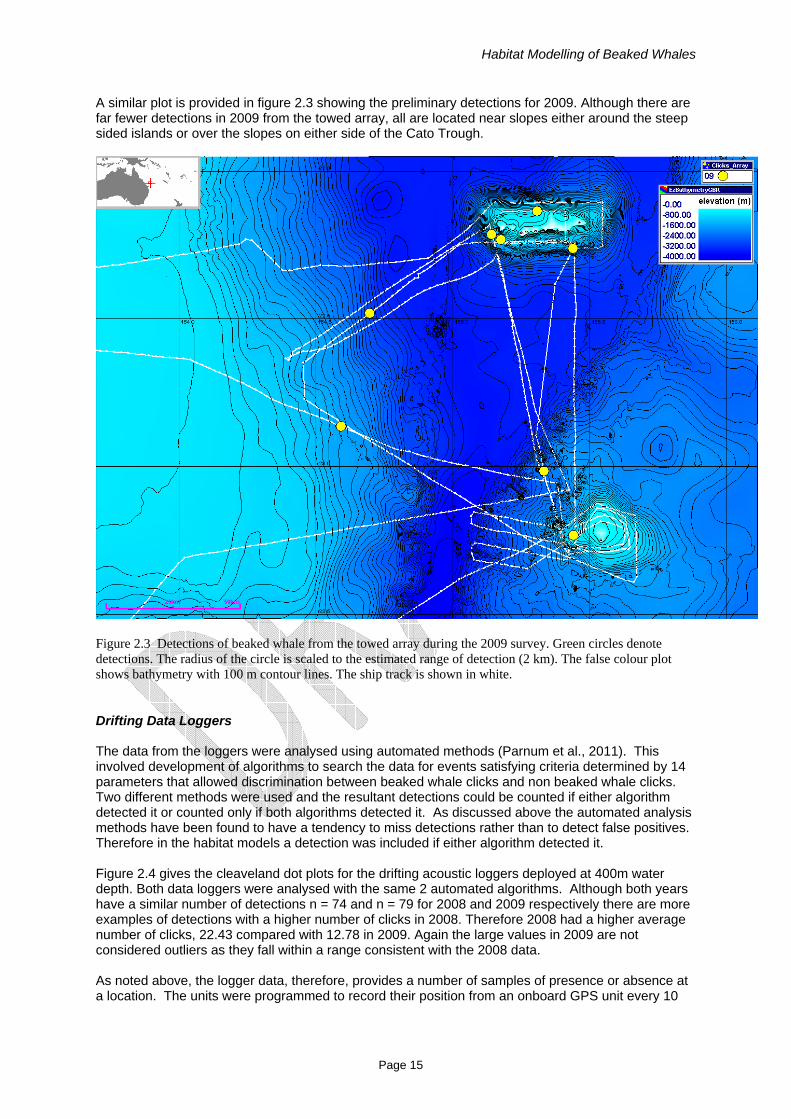
A similar plot is provided in figure 2.3 showing the preliminary detections for 2009. Although there are far fewer detections in 2009 from the towed array, all are located near slopes either around the steep sided islands or over the slopes on either side of the Cato Trough.

Figure 2.3 Detections of beaked whale from the towed array during the 2009 survey. Green circles denote detections. The radius of the circle is scaled to the estimated range of detection (2 km). The false colour plot shows bathymetry with 100 m contour lines. The ship track is shown in white.

Drifting Data Loggers The data from the loggers were analysed using automated methods (Parnum et al., 2011). This involved development of algorithms to search the data for events satisfying criteria determined by 14 parameters that allowed discrimination between beaked whale clicks and non beaked whale clicks. Two different methods were used and the resultant detections could be counted if either algorithm detected it or counted only if both algorithms detected it. As discussed above the automated analysis methods have been found to have a tendency to miss detections rather than to detect false positives. Therefore in the habitat models a detection was included if either algorithm detected it. Figure 2.4 gives the cleaveland dot plots for the drifting acoustic loggers deployed at 400m water depth. Both data loggers were analysed with the same 2 automated algorithms. Although both years have a similar number of detections n = 74 and n = 79 for 2008 and 2009 respectively there are more examples of detections with a higher number of clicks in 2008. Therefore 2008 had a higher average number of clicks, 22.43 compared with 12.78 in 2009. Again the large values in 2009 are not considered outliers as they fall within a range consistent with the 2008 data. As noted above, the logger data, therefore, provides a number of samples of presence or absence at a location. The units were programmed to record their position from an onboard GPS unit every 10


minutes. The GPS tracks of each drifting logger are displayed in figure 2.5 along with the beaked whale detections.

Figure 2.4 Cleaveland dotplots for detections from the drifting hydrophone loggers in both 2008 and 2009. Value represents the number of clicks per detection.

Figure 2.5 Beaked whale detections by the drifting data loggers deployed at 400 m depth for both the 2008 and 2009 survey. Tracks of the loggers are shown in white. The background plot is a false colour image of bathymetry with 100 m contours.


2.2. HABITAT PREFERENCE MODELLING

2.2.1. Environmental Analysis System / the Pelagic Habitat Analysis Module The Environmental Analysis System (EASy) software distributed by System Science Applications and developed at the University of Southern California is a fully 4 dimensional GIS designed specifically for marine applications. All data input to the GIS is stored by time, latitude, longtitude and depth. The EASy software is extendable by various services which can be loaded from within the software and which add various functionalities to the GIS, such as modelling capabilities or the ability to perform spatial statistical analyses. One such service is the Pelagic Habitat Analyses Module (PHAM) which was used extensively during this project for the collation of data as well as storage, manipulation, matching, and extraction of environmental datasets for the Beaked Whale study. The PHAM is a currently funded development project with funding from NASA’s decision support program (www.phamlite.com). It is a collaboration between a number of institutions including the University of Southern California (USC), the National Aeronautics and Space Administration of the USA (NASA), the South West Fisheries Science Centre, of the USA (SWFSC), the Inter American Tropical Tuna Commission (IATTC), and System Science Applications, of the USA (SSA). The PHAM is designed to merge fisheries / survey data with satellite imagery and circulation models to assist in the characterisation and mapping of pelagic species (Kiefer et al., 2009). During the research and development stage the PHAM has been successfully applied to pelagic habitat studies of tuna in the East Pacific Ocean (Harrison et al., 2010) and Sharks of the California Current system (Harrison et al., 2009). For the study of Beaked Whales in the region around Cato Island the EASy GIS was able to provide a home for all categories of data that were collected for the habitat study. These included: survey ship tracks, tracks of the drifting data loggers, detection data both for the towed hydrophone arrays and the drifting data loggers, raster and vector GIS data such as bathymetry and bathymetry derived variables, satellite remotely sensed data such as chlorophyll-a, sea surface temperature, sea surface altimetry, and circulation model output such as that from the Bluelink Ocean Circulation model which was used in this project, and environmental data collected during the survey from CTD and XBT casts, as well as underway temperature sampling at 400m depth by the drifting data loggers. The PHAM service was particularly useful in providing the ability to data-match the various dependent and independent data types and formats, as well as to create dynamic reconstructions of the cruise, visualise statistical relationships between the variables, organise and export data for statistical analysis and modelling outside of the GIS and re-import data for dynamic visualisation and geographic display of the results.

2.2.2 ESRI Arc GIS Arc GIS distributed by ESRI (www.esri.com) is a popular software for GIS applications within academia and industry. Although Arc GIS provides excellent tools for managing and storing geographic data, historically the application has lacked adequate tools for user friendly handling of time variant data such as satellite imagery or the output from ocean circulation models, although the latest edition incorporates new features to address these problems. Arc GIS has an immense user community and many add on packages and tool boxes which extend its capabilities, some of which were used during this project. Arc GIS was used during the beaked whale study to perform specific tasks such as calculating the slope and aspect of raster bathymetry. Additionally Arc GIS offers some modelling packages that were applied in this project to develop models of Beaked Whale habitat including Maxent. To facilitate the modelling activities in Arc GIS, a project was created for this study using data that was prepared in EASy GIS and output in formats compatible with Arc GIS.


2.2.3 Habitat models Species-environment studies investigate the general environmental characteristics related to the distribution of a particular species (Heglund, 2002). Underlying species - environment models is the assumption that predictable relations exist among the occurrence of a species and certain features of its environment (Heglund 2002; Guisan et al. 2006). These models are based on various hypotheses concerning how environmental factors influence the occurrence of species and communities (Guisan and Zimmermann 2000). Predictive habitat models provide a prediction of occurrence for a species by relating a set of presence localities to relevant environmental variables (Phillips et al. 2006). Methods for predictive habitat modelling often require presence/absence or abundance data from systematically designed surveys. For marine mammals the collection of absence data can often be difficult and expensive particularly over large spatial scales. Predictive models of species distributions can be created using varying statistical techniques. Absence of detection does not necessarily mean that the habitat is unsuitable. Habitat could be suitable but the animal is not there because it moves between habitats, or it is there but the detection cue (e.g. vocalisation, surfacing) is not detected (e.g. it is not vocalising or it is submerged). Frequently used techniques include Bayesian probability, Generalised Linear Models (GLMs), Generalised Additive Models (GAMs), Environmental Envelopes (EEs), Classification and Regression Trees (CART), Ecological-niche Factor Analysis (ENFA: Hirzel, 2002, 2008) and ordinations such as Artificial Neural Networks (ANNs) (Guisan and Zimmermann 2000; Guisan and Thuiller 2005). Significant differences between modelling techniques exist, including the amount of data required, the selection of predictive variables, outputs (e.g., presence/absence, probability of presence or abundance of the organism), statistical rigor, ease of interpretation of the models, and the amount of statistical and biological knowledge necessary to understand and apply the models (Guisan and Zimmermann 2000). Three models are investigated for determination of the habitat preferences of the beaked whales within the survey area. The first is the simple approach of taking histograms of detections for each of the environmental variables used. The second was a generalised linear model (GLM) using the presence/absence of beaked whales. The third was Maximum Entropy (Maxent: Phillips et al., 2004, 2006, 2008) using detections (i.e. presence only).

2.2.4 Compiled Datasets Several differing datasets were prepared for exploratory analysis and use in the habitat mapping models.

Beaked whale detections We define a “beaked whale detection” as a detected train of clicks. These are continuous trains and could be considered as the raw data of detection. Many detections were less than 1 s in duration, some were of order seconds and the longest was about 30 s. For the reasons discussed above, many detections may come from the same individual, so that the number of detections do not give an indication of the number of whales detected or the number of whale presences detected. Each detection of a beaked whale was loaded into the EASy GIS using the location of the ship or drifting buoy at the time of detection. The PHAM was then used to retrieve each associated variable at the same location and time from the environmental datasets previously loaded and geo-referenced in the GIS. For temporally varying variables, the resolution of the environmental data were either once daily or 8 daily. The value for each variable was taken as the value of the pixel over which the detection was made from the dataset with a temporal period within which the time of detection fell. For temporally invariant variables, such as water depth the value was simply taken as the value of the pixel on which the detection fell.


Presence / Absence Detection data were clustered into segments of 30 min of recording, each segment being considered as an area of beaked whale presence, as described in 2.1.2. The data were then handled somewhat differently by the two GIS systems. For the GLM model run in ‘R’ with the output from the EASy GIS the mid point of each segment were imported to the GIS and the data matching of environmental variables was conducted as described above for the presence only data. In Arc GIS the individual line segments were loaded into the GIS as vector data and sampling of environmental data was performed by extracting the pixels over which the segment line passed. Time variant environmental data could not be processed at its native temporal resolution in Arc GIS. It was necessary for the models run within Arc GIS to temporally average the daily or 8 daily raster images to create a single image layer representing that variable, which could then be used in the models. For the drifting data loggers it is more difficult to determine an appropriate segment length. In 2008 the drifting loggers had an average speed of 0.17 m/s, at which speed they would take around 13 hours to travel 8 km, during which time a whale may have entered and left the detection range, and or made multiple dives. The assumption of a stationary whale relative to the sampling platform is no longer valid. Unfortunately little is known about the swimming speed and movements of beaked whales in general and nothing is known concerning their movements within the current study area, the time spent in any one location may also depend on many behavioural factors, for example wether prey is present or not. From electronically tagged beaked whales of species Culvier’s (Ziphius cavirostris) and Blainville’s (Mesoplodon densirostris) it was observed that a typical dive lasts from 40 to 60 minutes (Tyack et al., 2006). For the sake of simplicity the segment length was also kept at 30 minutes for the drifting data loggers. At this segment length tests of the detection data failed to show conditional independence. If a detection was made in the previous segment, there was a higher probability of a detection in the following segment further discussion of this issue can be found in section 3.2. For this reason it was necessary to exclude the logger data from habitat analysis requiring presence / absence data. The logger data are therefore more suited to a presence only modelling approach at the current time. More work is needed to establish an appropriate segment length or division that may permit improved incorporation of the logger data into the presence / absence model types.

Figure 2.6. Graph of the autocorrelation function of presence/absence for the towed array, showing that there is no obvious correlation between successive samples (segments of the track). Lag is 10log10(segment number).


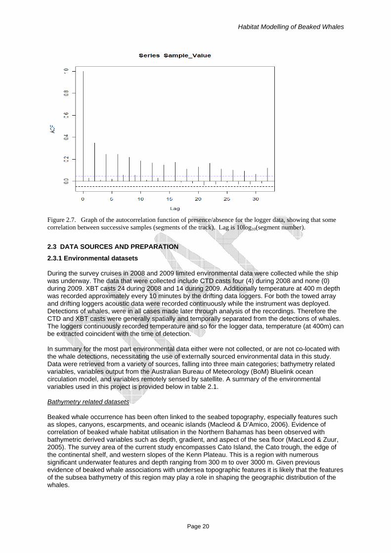
Figure 2.7. Graph of the autocorrelation function of presence/absence for the logger data, showing that some correlation between successive samples (segments of the track). Lag is 10log10(segment number).

2.3 DATA SOURCES AND PREPARATION

2.3.1 Environmental datasets During the survey cruises in 2008 and 2009 limited environmental data were collected while the ship was underway. The data that were collected include CTD casts four (4) during 2008 and none (0) during 2009. XBT casts 24 during 2008 and 14 during 2009. Additionally temperature at 400 m depth was recorded approximately every 10 minutes by the drifting data loggers. For both the towed array and drifting loggers acoustic data were recorded continuously while the instrument was deployed. Detections of whales, were in all cases made later through analysis of the recordings. Therefore the CTD and XBT casts were generally spatially and temporally separated from the detections of whales. The loggers continuously recorded temperature and so for the logger data, temperature (at 400m) can be extracted coincident with the time of detection. In summary for the most part environmental data either were not collected, or are not co-located with the whale detections, necessitating the use of externally sourced environmental data in this study. Data were retrieved from a variety of sources, falling into three main categories; bathymetry related variables, variables output from the Australian Bureau of Meteorology (BoM) Bluelink ocean circulation model, and variables remotely sensed by satellite. A summary of the environmental variables used in this project is provided below in table 2.1. Bathymetry related datasets Beaked whale occurrence has been often linked to the seabed topography, especially features such as slopes, canyons, escarpments, and oceanic islands (Macleod & D’Amico, 2006). Evidence of correlation of beaked whale habitat utilisation in the Northern Bahamas has been observed with bathymetric derived variables such as depth, gradient, and aspect of the sea floor (MacLeod & Zuur, 2005). The survey area of the current study encompasses Cato Island, the Cato trough, the edge of the continental shelf, and western slopes of the Kenn Plateau. This is a region with numerous significant underwater features and depth ranging from 300 m to over 3000 m. Given previous evidence of beaked whale associations with undersea topographic features it is likely that the features of the subsea bathymetry of this region may play a role in shaping the geographic distribution of the whales.


Table 2.1 Table of environmental variables used in the beaked whale habitat study Variable GIS Variable Code Source Units Spatial

Resolution

Temporal Resolution

Method of estimation

Bathymetry EzBathymetry3DGBR Project 3dGBR m 100 m N/A Measurement

/ Interpolation Aspect BWAspect Calculated

from 3dGBR Degrees from north

100 m N/A ArcGIS Toolbox

Slope BWSlope Calculated from 3dGBR

Degrees from horizontal

100 m N/A ArcGIS Toolbox

Current Zonal Bluelink_u BlueLINK m/s ~ 10 km Daily Modelled Current Meridonal

Bluelink_v BlueLINK m/s ~ 10 km Daily Modelled

Sea Surface Temperature

Bluelink_Temp BlueLINK °C ~ 10 km Daily Modelled

Sea Surface Height Anomaly (eta)

Bluelink_eta BlueLINK m from datum

~ 10 km Daily Modelled

Sea Surface Salinity

Bluelink_Salt BlueLINK psu ~ 10 km Daily Modelled

Sea Surface Temperature

EzGHRSST GHRSST °C ~ 25 km Daily Satellite / Interpolated

Chlorophyll-a EzChlorophyll SeaWiFS mg m-3 ~ 9 km Daily Satellite Chlorophyll-a EzCHL-MODIS MODIS-A mg m-3 ~ 4 km 8 Day Satellite Depth The Project 3DGBR gbr100 bathymetric dataset was selected for use in the Beaked Whale habitat study primarily because it offered the highest spatial resolution of gridded bathymetry encompassing the study region. The gbr100 dataset provided by ‘Project 3DGBR’ is a high-resolution bathymetry and Digital Elevation Model (DEM) covering the Great Barrier Reef, Coral Sea and neighbouring Queensland coastline. The DEM has a grid pixel size of 0.001-arc degrees (~100m) with a horizontal datum of WGS84 and a vertical datum of Mean Sea Level (MSL) (Beaman, 2010). The dataset is provided and maintained by James Cook University School of Earth and Environmental Sciences, Townsville, Australia. The grid provides high resolution bathymetry which is interpolated where necessary and is gap free, extending over the entire study region. The data are provided in both a vector format (contours) and raster format (gridded vales). Both data sets have been imported into the Beaked Whale project and are visible in the plot provided in figure 2.8 from the EASy GIS, the beaked whale rectangular survey grid is also shown. Cato Island appears in the South Eastern survey grid box. The dataset contains some visible artefacts although these do not noticeably extend into the survey region, an example is the two linear tracks of interference in the contour lines visible in figure 2.8 at 155.0° E and 21.5° S.


Figure 2.8. The 3DGBR100 bathymetric data for the beaked whale study area and surrounding waters. The elevation in meters is depicted by the false colour scale, contours are drawn at 100 m depth intervals. The horizontal resolution is approximately 100m. The coast of Queensland, Australia is visible in the lower left corner. Cato Island falls within the bottom right grid of the beaked whale study area.

Aspect Aspect of the sea floor slope was derived from the 3DGBR bathymetric dataset using Arc GIS 3D Analyst tool box. The aspect data were stored as a NetCDF raster and imported to the EASy GIS for analysis. Aspect reflects the directional facing of the slope across each pixel and is measured in degrees of bearing from North. The derived bathymetric aspect dataset used in this study is shown in figure 2.9. Slope Steepness of slope was likewise derived from the 3DGBR100 bathymetric dataset using the Arc GIS 3D Analyst toolbox. The slope represents the steepness in degrees of inclination from horizontal, with a value of 0 representing a horizontal surface. The slope of the survey area is shown in figure 2.10. Distance to 500m & 1000m depth To test for aggregation towards a favoured ocean depth in the survey area, the distance to 500 and 1000 m ocean depth contours were included. Arc GIS software was used to isolate the 500m depth contour from the 3D GBR 100 dataset and to calculate the Euclidian distance to the nearest point on a 500 m depth contour line. Figure 2.11 gives the results of this operation as loaded into the EASy GIS software. Distance to 1000m depth contour was calculated in the same manner and loaded into the GIS. A plot of the distance to 1000m depth dataset is not included here for brevity.


Figure 2.9. False colour image of seabed aspect derived from the 3DGBR100 bathymetric dataset, overlayed with contours of depth. The value is taken as the heading of the face of the slope across each pixel in degrees from North. The horizontal resolution is approximately 100m.

Figure 2.10. Slope of the seafloor derived from the digital elevation model. The slope is measured in degrees of inclination from horizontal for each pixel. The horizontal resolution is approximately 100m.


Figure 2.11. Distance to 500 m water depth. Distance is measured in degrees of longitude, one degree of longitude is roughly 100 km.

BLUElink circulation model data: currents, sst, sea surface height, salinity The BLUElink Ocean Model, Analysis, and Prediction System (OceanMAPS) is Australia’s ocean forecasting system operated by the Australian Bureau of Meteorology since August 2007, the background and details of the BLUELink project are given in Brassington et al. ( 2007) and Brassington et al. (2006). Bluelink OceanMAPS has a resolution of 0.1°×0.1° in the Asian Australian region (90E-180E, 75S-16N) which includes the survey area. The model assimilates satellite altimetry sea level anomaly from JASON1 and Envisat, satellite sea surface temperature from AMSR-E and in situ profiles including Argo and XBT casts. Fluxes are forced from the BoM’s operational global weather prediction system (Brassington et al., 2011). Near real time (5 days delay) ocean state estimates are produced by the model. Model technical specifications can be found online at http://www.bom.gov.au/oceanography/forecasts/technical_specification.pdf. The Bluelink OceanMAPS represents the highest resolution circulation model available for the region and temporal period of the beaked whale surveys. Output from the model was retrieved for the parameters of sea surface temperature (SST), sea surface height (SSH), Salinity, and the meridional and zonal components of current velocity at the surface. Output from the Ocean Forecast Australia Model (OFAM) anlaysis version 1.0 of the model was downloaded from the BoM servers using the OPeNDAP protocol (www.opendap.org) and subset using the open source NetCDF Operator (NCO) utilities (www. nco.sourceforge.net) which allowed daily raster images to be created and stored in NetCDF format for import to the GIS software. An example of each parameter on a single day (2-August-2008) during the survey is given below in figures 2.12 to 2.15. The currents in the model are output as separate raster images for the meridional and zonal vector components. The zonal component (labelled ‘u’) is the component of current in the East – West


direction with the convention that positive indicates current flow towards the east and negative indicates current flow towards the west. The meridional component (labelled ‘v’) represents flow in the North – South direction with the convention that Northward flow is represented as positive. The two components are loaded into the GIS in their native format and stored separately, a facility within the GIS allows the components to be combined and represented as vectors with magnitude and heading for display, as for example depicted in figure 2.12. However when data are output from the GIS, as each component is a separate layer the output is in terms of the individual components. In some cases where it aids interpretation post processing was applied to the results in this study to convert the components into magnitude (of velocity) and a compass heading indicating the direction of flow in degrees from North. Sea surface height anomaly (eta) is a two dimensional field of the ocean surface representing the difference in ocean surface height at each pixel from the long term average, figure 2.14. Sea surface height anomalies are associated with eddies and fronts which may potentially play a role in creating aggregations of beaked whale prey. The sea surface salinity is an indication of the salt density in the surface layer of the ocean and is estimated by the model in practical salinity units (psu), figure 2.15 is an example of the surface salinity on the 2/8/2008 near the beginning of the first beaked whale survey.

Figure 2.12 BLUELink Ocean Forecast Model Australia surface currents for 2-August-2008 during the 2008 survey. The arrows indicate direction of the current and the size and colour of the arrows represent the current magnitude in m/s. Note the anti-cyclonic eddy just to the South of the study area.


Figure 2.13 BLUELink Ocean Forecast Model SST for 2-August-2008 during the 2008 survey. This image is for the same date as the current velocities shown in figure 2.12. Sea Surface temperature is given in degrees Celsius. Horizontal resolution of the BlueLINK model is around 10 km.

Figure 2.14 BLUELink Ocean Forecast Model sea surface height anomaly ‘eta’ in meters for 2-August-2008 during the 2008 survey. An anti-cyclonic eddy appears just South of the study area. In the colour scale blue represents ‘0’ sea level height anomaly, shades of green positive and shades of red negative. Horizontal resolution is approximately 10 km.


Figure 2.15 BLUELink Ocean Forecast Model surface salinity in practical salinity units (psu) for 2-August-2008 during the 2008 survey.

Satellite derived datasets: Chlorophyll-a Remotely sensed satellite data were incorporated into the project both to corroborate data from the BLUELink model and to provide parameters that are not included in the model. Estimated Chlorophyll-a data were imported from both the SeaWiFS and MODIS-A satellite sensors. SST was obtained from the Group for High Resolution Sea Surface Temperature (GHRSST) product, a daily global gap free interpolation of satellite derived data with the argo drifting buoy network. These two datasets were downloaded from the NASA PODAAC ftp site.

GHRSST: Sea surface temperature The Group for High Resolution Sea Surface Temperature is a follow on from the Global Ocean Data Assimilation Experiment (GODAE) taking over from the GODAE high resolution SST pilot project in 2009. The stated aim of the GHRSST is “to provide the best quality sea surface temperature data for applications in short, medium and decadal/climate time scales in the most cost effective and efficient manner through international collaboration and scientific innovation” (www.ghrsst.org). The advantages of the GHRSST product over other SST products derived from individual satellite instruments is that it provides a global daily gap free dataset, which incorporates interpolation between satellite sensors and data from the ARGO drifting buoy network. For the beaked whale project the data are of a relatively low spatial resolution (~25 km) compared with the size of the study area (approx 170 km x 110 km). For this reason the habitat modelling will rely primarily on the higher resolution outbut of the Bluelink model, the GHRSST imagery was included for comparison with the modelled SST. The GHRSST data are provided in NetCDF format which is readily imported to EASy and scaled within the software to give physical pixel values of SST in °C.

Chlorophyll-a Estimates of chlorophyll-a concentration in the upper ocean were downloaded from two satellite mounted sensors, SeaWiFS and MODISA. For both sensors it was necessary to download the entire


global grid for each timestep. The global grids were imported into EASy and then the sub setting and export tool was used to subset the images for a spatial region encompassing the survey area and surrounding ocean. A region larger than the survey area was selected so that in the final stages of the project when the modelling results were applied to create predictions of the habitat they could be extended over the surrounding region. The subset raster imagery was converted and exported from EASy in NetCDF format so that it could also be readily imported to the ArcGIS project. The imagery was then reimported both into EASy and ArcGIS, using the subset images allowed for faster processing and lower disk space requirements. Initially it was planned to use daily chlorophyll data and this was obtained from the SeaWiFS sensor at 9 km spatial resolution. However examination of the data in the survey area revealed that there were very little useable data due to cloud cover. The MODISA product in 4 km spatial resolution formed into 8 day composites provided far better coverage, virtually eliminating missing data due to cloud cover in the region of interest. Unfortunately this came at the cost of reduced temporal resolution with only 4-5 images per survey period. For illustration figure 2.16 shows a daily SeaWiFS chlorophyll image from the 1/3/2009.

Figure 2.16 A raster plot of estimated chlorophyll on the 1/3/2009 from the SeaWiFS satellite sensor. There are no data values for significant areas due to cloud cover. This is one of the best daily images available during the survey periods. The false colour image is presented in µg/m3 of cholorphyll-a.


3. RESULTS 3.1 DETECTIONS Figure 3.1 shows all detections of beaked whales and their locations during the surveys in 2008 and 2009. The detections symbols are scaled to approximately represent the range of detection, centred at the location of the ship / drifting logger at the time of detection. A visual inspection reveals an apparent clustering around the steep sided islands / reefs as well as the slopes of the Cato Trough. There appear to be fewer detections over the abyssal plain, particularly where it widens to the North. The number of detections for each sensor type and for each survey are given in table 3.1. The environmental data associated with each detections is summarised by frequency histograms in figure 3.2. Data for 2008 and 2009 were lumped together in the histograms for the towed array since there are so few detections identified in 2009 at the current time.

Figure 3.1 The location of detections of beaked whales from the towed hydrophone array and the drifting hydrophone data loggers during the surveys in 2008 and 2009. Table 3.1 Summary of the numbers of detections and 30 minute segment presence absence data used in the habitat modelling. Sensor Year Total

detections Number of 30 min segments

Number presence segments

Fraction with presence

Towed Array 2008 212 411 21 5.12 % Drifting Logger 2008 74 960 61 6.35 % Towed Array 2009 8 343 8 2.33 % Drifting Logger 2009 79 741 58 7.83 %


Figure 3.2 Histograms of the detections during the beaked whale cruises in 2008 and 2009. Data from both the drifting data loggers and the towed arrays are displayed. For the towed array 2008 and 2009 detections were lumped together due to the small amount of detections so far identified in 2009. Unfortunately the detailed analysis of the 2009 data was not available for this study. Total number of detections for each data type are given in table 3.1.


3.2 GENERALISED LINEAR MODEL OF PRESENCE/ABSENCE A generalized linear model was used to analyse the presence or absence of beaked whale detections using the acoustic data collected from the towed array. A “detection” means that beaked whale clicks were detected within the 30 min segment of the towed array track, and thus beaked whale presence was counted for that segment. If no clicks were detected within a segment, it counted as an absence. A presence/absence model (1, 0) involves the Binomial distribution. There are 4 conditions of this distribution which must be met:

1. There are only two outcomes (satisfied if this analysis), if clicks are available to be detected, they are detected at each site (1) (almost satisfied in this dataset i.e. it is likely that clicks are detected at most sites where available: see section 2.1.2), no acoustic detections translates to click absences (0) (mostly satisfied in this dataset)

2. There are a fixed number of trials (each half hour segment has been designated a ‘site’ or ‘trial’, and is satisfied in this analysis)

3. Observations are independent, in other words half hour segments can be viewed as independent trials. Therefore the probability of detecting clicks in a half hour segment does not increase if a click was detected in the previous half hour segment (satisfied: tested by calculating the autocorrelation function to see if there is any evidence of autocorrelation within successive samples – see below)

4. There is a constant probability of success (assumed for this analysis and there is no reason to assume otherwise).

Each 1, 0 value within the presence/absence data represents a half hour bin or segment of the array track. To test if each half hour segement could be considered as an independent sample, a plot of the similarity between observations as a function of the time separation between them was used to assess the serial dependence of samples, see graph below. This found no evidence of autocovariance between successive segements (Fig. 3.3). Therefore, for this analysis, each half hour segment can be treated as an independent sample (in terms of the probability of detecting clicks in successive segment based on click detection in the previous half hour bin or segment).

Figure 3.3. Graph of the autocorrelation function shows that there is no obvious increase in detection probability with a decrease in the lag between successive samples (segments of the track). Lag is 10log10(segment number).


3.2.1. Data exploration For this dataset, there were 584 samples (segments) in which clicks were not detected and 28 samples in which clicks were detected for the 2008 and 2009 array dataset. This is a very low sample size and therefore modelling for predictor variables may be difficult. The graphs in Fig. 3.4 show the probability of beaked whales presence detected within a segment with 6 of the measured environmental variables, from the distribution of the data (effectively normalized histograms). From first glance, it seems that temperature has an effect on click detection in that clicks are more likely to be detected in a lower sea surface temperature and possibly the slope of the sea floor (clicks are more likely to be detected near higher slopes).

Figure 3.4. Probability of presence of beaked whales based on detecting clicks in a segment (labelled as probability of click detection) for six variables plotted from the distribution of the data.


Replotting the data as boxplots of (median number of ‘presence’ samples and ‘absence’ samples) indicates clicks are more likely to be detected in lower SSTs, increased slope of the sea floor and there may be some affect of the distance to the 500m contour (Fig. 3.5).

Fig. 3.5 . Boxplot of the range of values of some variables for presence and absence of clicks within a segment. Each box shows the median bounded by the 1st quartile (25th percentile) and the 3rd quartile (75th percentile). The lines outside the boxes are 1.5 IQR (interquartile range) above the 3 quartile or below the 1st quartile.


3.2.2. Model selection and comparison An additional time variable was added to the dataset before model selection and comparison. Each sample was categorized according to the time the sample was taken – 00:00 – 06:00, 06:01 – 12:00, 12:01 – 18:00, 18:01 – 23:59. Table 3.2 . Predictor variable codes used in the GLM descriptions of each code are given in table 2.1. Sample_Value Sample_Bluelink_eta Sample_BlueLink_Salt Sample_Bluelink_Temp Sample_Bluelink_u Sample_Bluelink_v Sample_BWAspect Sample_BWSlope Sample_Dist1000m Sample_Dist500m Sample_EzBathymetryGBR Sample_EzChlorophyll Sample_EzGHRSST Sample_EzCHL.MODIS Time The full model including all predictor variables apart from an estimation of chlorophyll levels (Sample_EzChlorophyll) which had too many missing values and was therefore replaced by Sample_EzCHL.MODIS (which used 8 day composites and therefore had less blanks) is: fit1<-glm(Sample_Value~ Sample_Bluelink_eta+ Sample_BlueLink_Salt + Sample_Bluelink_Temp + Sample_Bluelink_u + Sample_Bluelink_v + Sample_BWAspect + Sample_BWSlope +Sample_Dist1000m + Sample_Dist500m + Sample_EzBathymetryGBR + Sample_EzCHL.MODIS + Time, family=binomial, data=array) Stepwise selection takes a step wise approach in model selection where the deviance of each model is compared to determine which combination of variables are most likely to predict the presence/absence dataset. Each iteration is reported and the final model in the process is determined to be the ‘best’ model. The ‘best’ model is then selected for further exploration. When taking this approach the best model (in terms of Akaike Information Criterion (AIC) scores) contained a number of predictor variables. However, this predictor model included two measures of SST: bluelink and daily global gap free interpolation of satellite derived data with the argo drifting buoy network (Sample_EzGHRSST). The residual deviance indicated that the bluelink temperature was the better predictor variable in the model, therefore the Sample_EzGHRSST was removed and the step wise analysis re-ran (termed ‘fit1b’ as the initial full model not including Sample_EzGHRSST). The best model (fit 2) in terms of AIC score comparisons was a model that included measures of temperature, salinity, aspect, distance to the 1000m contour, chlorophyll and time detailed below: fit2<- glm(Sample_Value ~ Sample_Bluelink_Temp, Sample_BlueLink_Salt, Sample_BWAspect, Sample_Dist1000m, Sample_EzCHL.MODIS, Time, family=binomial, data=array) df AIC AICc fit1b 15 221.2 222.0 fit2 9 211.0 211.3


Table 3.3 illustrates the reduction of the residual deviance by the sequential addition of each predictor variable and shows that most of the deviance is explained by the variation in sea surface temperature. Table 3.3. Reduction in residual deviance by sequential addition of each predictor variable. Df Deviance Resid. Df Resid. Dev NULL 611 227.433 Sample_BlueLink_Salt 1 1.384 610 226.048 Sample_Bluelink_Temp 1 16.417 609 209.631 Sample_BWAspect 1 3.567 608 206.064 Sample_Dist1000m 1 4.334 607 201.730 Sample_EzCHL.MODIS 1 0.776 606 200.9 3 Time 3 7.974 603 192.980 Likelihood ratio tests were used to test the difference in deviance (amount of variability explained by each model) between each fit using a chi-squared distribution. The test compares twice the difference between the log-likelihood values with a chi-squared distribution with the df equal to the number of parameters used to fit the models. A significant value indicates that the reduced model is unlikely to have generated the data. Likelihood ratios between the full and reduced model were compared: Response: Model (fit 1b or fit 2) LR difference Df Pr(>Chisq) Model 2.750964 16 0.9 and the non-significant result indicates that the reduced model is more likely to have generated the data. In other words, there is a high chance of getting this chi-squared value if the null (a high probability that the reduced model generated the data compared to the full model) is true. Likelihood ratio tests were also performed to determine if each variable had one or more non-zero coefficients and therefore should be retained (Table 3.4). Therefore, the results suggest the reduced model is a much better predictor of the beaked whale presence/absence data than the full model and that sea surface temperature, the distance to the 1000m contour and time are potentially significant (p<0.05) predictor variables for beaked whale distribution.


Table 3.4. Likelihood ratio tests on each variable to test which had one or more non-zero coefficients and therefore should be retained. Anova Table (Type II tests) Response: Sample_Value LR Chisq Df Pr(>Chisq) Sample_Bluelink_Temp 4.5995 1 0.03198 * Sample_BlueLink_Salt 2.3235 1 0.12744 Sample_BWAspect 2.0289 1 0.15433 Sample_Dist1000m 6.5736 1 0.01035 * Sample_EzCHL.MODIS 2.7393 1 0.09790 . Time 7.9735 3 0.04656 * Signif. codes: 0 ‘***’ 0.001 ‘**’ 0.01 ‘*’ 0.05 ‘.’ 0.1 ‘ ’ 1

Figure 3.6. Probability of presence of beaked whales (labelled as probability of click detection) from the distribution of data for the three variables found to be significant predictors (p < 0.05). Probability of click detection increases with a decrease in sea surface temperature, a decrease in distance to the 1000m contour and clicks are more likely to be detected in the daytime (between the hours of 06:00 and 12:00).


3.2.3. Model Interpretation The following is the summary of the coefficients of the model: Coefficients: Estimate Std. Error z value Pr(>|z|) (Intercept) 105.803662 62.709373 1.687 0.0916 Sample_Bluelink_Temp -0.729159 0.356366 -2.046 0.0407* Sample_BlueLink_Salt -2.527043 1.583414 -1.596 0.1105 Sample_BWAspect 0.003006 0.002142 1.403 0.1605 Sample_Dist1000m -4.259603 1.766868 -2.411 0.0159* Sample_EzCHL.MODIS -9.890925 6.253870 -1.582 0.1137 Time06:00-12:00 1.132527 0.579860 1.953 0.0508 Time12:00-18:00 0.521331 0.633727 0.823 0.4107 Time18:00-00:00 -0.440087 0.698564 -0.630 0.5287 Signif. codes: 0 ‘***’ 0.001 ‘**’ 0.01 ‘*’ 0.05 ‘.’ 0.1 ‘ ’ 1 (Dispersion parameter for binomial family taken to be 1) Null deviance: 227.43 on 611 degrees of freedom Residual deviance: 192.98 on 603 degrees of freedom AIC: 210.98 Number of Fisher Scoring iterations: 7 The R2 value was also calculated for this model and found to be 0.194 (which is quite low). Under the model (not including ‘time’ which is a factorial predictor variable), we would expect to detect about 2 presences for every 100. In other words, the probability of detection for mean values of temperature, salt, aspect, distance to 1000 m and chlorophyll is approximately 0.02. However, clicks are also more likely to be detected between the hours of 06:00 and 12:00 and therefore the probability of detection will increase during this time.

3.2.4. Summary of findings In summary, the analysis shows quite strong evidence that the probability of detecting the presence of beaked whales using clicks from a towed array increases with a decreased sea surface temperature. The analysis also shows that the probability of detecting presence increases with a decreased distance to the 1000 m contour and is more likely between the hours of 06:00 and 12:00 with weak evidence that detections are also related to salt, aspect and chlorophyll. However, the sample size for ‘presence’ was quite low compared to ‘absence’ and with more ‘presence’ data, model fit may be improved and other variables may become more significant. Further work suggested:


1. Re-doing this for the logger data and include the logger data in the model to increase the sample size of detections.

2. Attempt a presence-only type approach (as click absence does not necessarily equate to animal absence and clicks that are available for detection may not have been detected from the array).


3.3 APPLICATION OF MAXENT FOR PREDICTING BEAKED WHALE PRESENCE

3.3.1 Background The Maxent program models species distributions from presence-only species observation records. Maxent uses maximum entropy techniques and can perform well with small numbers of species observations (Phillips et al., 2004). The model was applied to estimate the probability of beaked whale presence conditioned on six selected non-time variant environmental variables. It is important to consider the selection of landscape (study area extent), species data and environmental conditions when applying the Maxent model as these will influence the results. The study area was defined within the 2008 and 2009 survey plots to ensure predictions were within the range of the training data and that covariate data (geomorphology) was available across the modelled landscape.

Figure 3.7 Map showing the area used in the Maxent modelling. The advantage of the current study is that there is a temporal and spatial scale associated with the beaked whale occurrence data defined by the array swath and observation time. This should be exploited in the type of model selected. A spatial resolution or sampling unit size of 110 m was defined based on the spatial resolution of the covariate data sets. All GIS datasets were projected into MGA94 Zone 56 projection for use in the model. Although Maxent’s predictive performance has been demonstrated to be high (Elith et al., 2006), it is recommended that if presence-absence survey data are available it is advisable to use a presence-absence modeling method which is less susceptible to problems associated with sample selection bias (Elith et al., 2011).


3.3.2. Model outputs The logistic output from the Maxent model estimates probability of presence based on the assumption that typical presence localities have a probability of presence of about 0.5 (depending on sampling design). Environmental variables used in this model include bathymetry, aspect, slope, Euclidean distance to reef, Euclidean distance to canyons and Euclidean distance to the continental shelf. The mapped predicted probability of suitable conditions for beaked whales within the Cato Island study area is shown in Figure 3.8. The probability value assigned to each grid cell (pixel) is small as the values must sum to 1 over all cells in the raster so these are not “probability of occurrence” values (Phillips, 2011).

Figure 3.8. Predicted probability of suitable conditions for beaked whales. Red-orange indicates high probability of suitable conditions for beaked whales, green indicates conditions typical of where they have been recorded and light blue indicates low predicted probability of suitable conditions. White points indicate presence samples used in training the model (2008 array data) and purple points indicate test samples (2009 array data) used to test the model. The arcs near the centre of the map may reflect clustering of detections at the same distances from the islands.


3.3.3. Evaluating model performance These results indicate the omission rate and predicted areas as a function of the cumulative threshold calculated on the training (2008 array data) and test (2009 array data) species presence records (Phillips, 2011). Binomial tests require that thresholds are used to convert continuous predictions derived from Maxent into binary predictions delimiting the suitable versus unsuitable areas for beaked whales (Phillips et al., 2006). The threshold is used to make a binary prediction. Suitable conditions (for whale habitat preference) are predicted above the threshold and unsuitable below the threshold (Phillips, 2011). Figure 3.9 shows that the omission on test samples (drawn from the 2009 array data) is a reasonable match to the predicted omission rate. This graph is useful for identifying potential sample bias. In this case the test and training data should be independent as they were sampled during different survey trips and it is assumed they are not spatially autocorrelated.

Figure 3.9. Omission and predicted area for beaked whale using the 2008 array data to train the model and the 2009 array data to test the model. The omission predicted area shows the relationship between predicted values of occurrence probability and the proportion of occurrences selected. The receiver operating characteristic (ROC) curve plots true positive rate against false positive rate for each threshold and the area under the ROC curve (AUC) is the probability that the classifier correctly orders a set of random positive and negative samples. The red line shows the “fit” of the model to the training data (2008 array data) and the blue line shows the “fit” of the model to the testing data indicating the models predictive power (Phillips, 2011). The black line shows what would be expected if the model was no better than random. The closer towards the blue line is to the top left of the graph, the better the model is at predicting the presences contained in the test sample data (Phillips et al., 2004). In figure 3.10 the blue line (test data) increases steeply indicating a good model. The AUC value of 0.981 is high indicating strong model performance in discriminating suitable versus unsuitable areas for beaked whales. Based on the null hypothesis that test points are predicted no better than by a random prediction with the same fractional predicted area, binomial test were performed. Model performance can be examined using omission rate, the fraction of test samples (2009 array data localities) that occur in grid cells (pixels) not predicted as suitable for the species (Phillips et al., 2006). The binomial omission test was significant (p<0.001). The omission rate ranged from 12.5 to 50% (Table 3.5).


Figure 3.10.. Receiver operating characteristic (ROC) curve showing the model performance in predicting beaked whale occurrences compared to randomly selected points. Sensitivity is the proportion of presence localities correctly predicted. Fractional Predicted Area is the proportion of all grid cells (pixels) in the study area predicted to have suitable conditions for beaked whales. Table 3.5. Fractional predicted area and omission rate for common Maxent thresholds. Fractional predicted area is the fraction of all grid cells predicted as suitable for beaked whales. Omission rate is the proportion of the test samples (2009 array data) occurring outside the prediction. Cumulative threshold

Logistic threshold

Description Fractional predicted

area

Training omission

rate

Test omission

rate

P-value

1.000 0.007 Fixed cumulative value 1 0.359 0.000 0.125 4.227E-3



2.025 0.013 Minimum training presence 0.286 0.000 0.125 9.446E-4

18.388 0.159 10 percentile training presence

0.044 0.099 0.500 2.29E-4

13.510 0.084 Equal training sensitivity and specificity

0.070 0.070 0.500 1.365E-3

16.262 0.122 Maximum training sensitivity plus specificity

0.053 0.070 0.500 4.731E-4

4.801 0.027 Equal test sensitivity and specificity

0.188 0.021 0.250 8.693E-4

4.799 0.027 Maximum test sensitivity plus specificity

0.188 0.021 0.125 5.538E-5

4.332 0.025 Balance training omission, predicted area and threshold

value

0.200 0.007 0.125 8.386E-5

13.765 0.086 Equate entropy of thresholded and original distributions

0.069 0.070 0.500 1.233E-3


3.3.4. Analysis of environmental variable contributions to the model The two methods for ranking the importance of environmental predictor variables are percentage contribution and permutation importance. As the Maxent model is being trained (optimization routine) it keeps track of the overall model gain and which environmental variables are contributing to fitting the model (Phillips, 2011). Each algorithm iteration increases the gain of the model by modifying the coefficient for a single feature, this gain is assigned to the environmental variable(s) on which that feature depends which is then converted to percentages (Phillips, 2011) which are shown in the second column in Table 2. When environmental variables are highly correlated caution should be used in the interpretation of percentage contributions. The contribution for each variable is determined by randomly permuting the values of that variable among the training points (both presence and background) and measuring the resulting decrease in training AUC (Phillips, 2011). The model is strongly dependent on a variable if it has a large decrease in training AUC. These values are normalized to provide percentages (Phillips, 2011). Bathymetry, Euclidean distance to reef and Euclidean distance to canyons are shown to be important environmental variables in this model (Table 3.6). Table 3.6. Analysis of variable contributions

Variable Percent contribution Permutation importance Euclidean distance to reef 46.7 27.7 Slope 18 3.5 Euclidean distance to canyon 15.6 21.2 Bathymetry 13 37.7 Euclidean distance to continental slope 4.6 8.7 Aspect 2.1 1.2

. The Jackknife test provides an alternative estimate of environmental variable importance and accounts for dependencies between environmental variables. Figure 5 shows results of the jackknife test. Euclidean distance to reef has the highest gain when used in isolation suggesting this variable allows a reasonably good fit to the training data.

Figure 3.11. The measure of model predictive ability is shown on the x-axis. Dark blue indicates model performance when only that environmental variable is used. Light blue indicates model performance when the environmental variable is excluded. Results of the jackknife test suggest that all environmental variables used in this model are appropriate predictor variables. Euclidean distance to reef has the highest gain when used in isolation and appears to have the most useful information by itself. This environmental variable also decreases the gain most when excluded, suggesting it has the most information that is not present in the other variables and has greater model importance. Response curves show how individual environmental variables influence the prediction. The probability of presence decreases with Euclidean distance from canyons and reefs (Figure 6).


Figure 3.12. Marginal response curves for each environmental variable when all other environmental variables are kept at the average sample value over the set of presence localities. Further considerations

• Time variant data sets were not included in this model due to data errors and should be incorporated in future applications of Maxent.

• It is important to consider whether the predicted distribution of species is biased by sampling effort. Sample selection bias, survey bias present in geographic space which will map into covariate space ( Elith 2011), has a stronger effect on presence-only models. In addressing potential survey bias it would be useful to examine spatial autocorrelation of samples using a statistic such as Moran’s I.

• The boundary of the study area should be reviewed as Maxent is a log-linear model (similar to GLM in form) and depends on both the presence samples and the background samples that are used in forming the estimate (Elith, 2011). Extending the study area


west to include the nearshore waters will alter the results and would need to be considered carefully in the absence of survey data in this region.

• Given the model is dealing with vagile species the influence of cell (pixel) size should be reviewed.

• Representation of aspect in degrees may be inappropriate and consideration should be given to representing aspect as a categorical variable or based on a selected direction (e.g. “northness”).

• Further work is needed to investigate the appropriateness of predicting to environments outside the range of training data (ie. broader Coral Sea region).

• The current results have not been considered in the context of species behaviour and habitat preference and there is a need to review the ecological relevance of predictor variables.


4. COMPARISON OF RESULTS AND CONCLUSIONS The environmental variables in the histograms showed more detections in:

• more saline water • cooler temperatures • shorter distance to 500 m and 1000 m water depth contours (< 3km) • current headings clustering around a south westerly direction.

There is a spread over water depths and sea floor slopes (see discussion below). There also appears to be clustering around lower values of chlorophyll-a, and lower sea surface heights. The GLM results, based on presence and absence data, showed that the best model included the following variables, in order of significance (most significant first):

• sea surface temperature (lower temperatures) • time of day (detections of presence more likely during daylight than at night) • distance to the 1000 m water depth contour (shorter distances) • aspect of sea floor slope (direction it faced) • salinity • chlorophyll-a

The Maxent model, based on detections, showed that all the variables used in the model are appropriate predictors of beaked whale detections, approximately in order of significance (Maxent model did not include time varying data):

• distance to reef (shorter) • sea floor slope or gradient re horizontal (steeper) • distance to canyons (shorter) • water depth (see discussion below) • distance to continental slope • aspect of sea floor slope

Distance to reef and slope appear to be the most important, distance to canyons, water depth and distance to the continental slope of similar importance, and aspect the least important. The results need to be carefully interpreted in the context of how representative the sampling is of the exercise area and the ocean in general in terms of possible beaked whale habitats, and the distributions of environmental variables. The results are dependent on the way the detections and presence of beaked whales were measured, whether the model used presence only or presence and absence, and how representative the survey paths were of the area in terms of the distribution of environmental variables. The “detections” in the histograms and the Maxent modelling are detections of contiguous click trains, not individual whales or presence areas. The GLM on the other hand used presence/absence data based on splitting the survey paths into 30 min segments. Each segment was considered as a presence of beaked whales within the area of localisation, i.e. the area over which a beaked whale could be detected acoustically. A presence was counted if there were one or more detections in the segment. There may be many detections and may be more than one whale in a segment. The Maxent model did not use estimates of absence but compared the distributions of detections for each environmental variable with the distribution of that variable across the whole area chosen for the model (the background data). This area is somewhat larger than the exercise area. In practice, the distribution across the area was randomly sampled. The area chosen is shown in Fig. 3.7. If the environmental variables along the paths taken during the survey are not representative of the distribution of those variables across the area, then this will bias the results from the histogram and from the GLM. The Maxent model avoids this by using data across the area, but the results will depend on the actual area chosen. In our modelling, we chose an area larger than the actual navy exercise area, to give a broader range of environmental variables. The choice of the area is likely to affect the results. The Maxent model does not include absences, though the use of background data


to some extent compensates for this in the Maxent model (sometimes referred to as pseudo-absences). The histograms simply compare the number of detections for the range of values of each environmental variable that applied at the time and place of the detections. Hence it is dependent on how representative the distributions of variables along the survey paths are of the whole area, and it is limited by not having absence data. The definition of a “detection” is also likely to affect the results, given that the duration of detections vary over a wide range. The definition of segment may also affect the results depending on how representative it is of the detection area. For the array, the lack of correlation between segments suggests that the definition is a reasonable choice for the array. There is some correlation between segments for the loggers as might be expected given the low speed at which they move. The array data generally sampled many segments within the time resolution of the environmental data (order one day). On the other hand, the loggers move slowly enough to provide some temporal sample for a small change in location on the scale of beaked whale dives (order one hour), and even on the temporal resolution of the environmental variables. Some indication of the importance of these biases and other effects might be obtained by varying the segment size in the presence/absence, basing the segment size on distance covered rather than time, clustering detections to some minimum duration, and varying the area used to provide the background information in the Maxent. In the last case, the question of what area should be used may depend on the purpose. If modelling is to be representative of the likely habitat within the navy exercise area, then perhaps this should be the area chosen for the background data. If the aim is to apply the model to predict probability of occurrence in other areas, the background data might be chosen from more general distribution of the environmental variables, but the applicability might be limited to areas where the range of values of these variables is similar to those surveyed. An example of how the choice of area can affect the results is evident in the sea floor slope or gradient. Although slope is detected as a significant variable, the dependence on slope is less than on some other variables. The histograms show that most detections are over slopes between 1° and 10° to the horizontal. The Maxent model shows it to be a significant predictor but the best GLM prediction did not include slope. The probability of presence as a function of slope from the Maxent model (Fig. 3.12) shows most presences would be expected to occur for slopes greater than about 4°. However, the distribution is broad above 4° so that this appears to be a limited predictor of presence. Sea floor slopes in the ocean are very small. Slopes or gradients of continental shelves are typically between 0.1° and 0.5°, while gradients of the abyssal plain of the deep sea floor, significantly less than that. Gradients of continental slopes are typically from 1° - 10° with that slope averages between 3° and 5°. When viewed in this context, the result that beaked whale detections are mainly over slopes of 4° or more, becomes much more significant than is evident from the analysis: the likelihood of presence is much higher over what would be considered to be steep slopes in the ocean, geographically limiting presence mainly to continental slopes, sides of canyons and the steeply sloping sides of oceanic islands. Continental shelves and the deep sea over abyssal plains are far less likely even though they cover a larger area of the ocean than the steeper sloping regions. The exercise area has a larger proportion of steeply sloping sea floor than is typical of the ocean (see Figs. 1.1 and 2.8). Within the exercise area, most of the survey paths in 2008 were over the eastern part where the slopes are higher. This is likely to bias the histogram and GLM results to showing a preference for higher slopes. The area used in the Maxent model has a distribution of slopes that is more representative of the ocean so should be less biased. Another variable for which the results may be misleading is the depths assigned to beaked whale detections and segments of presence/absence. The depth is taken to be the depth at the location recorder (the GPS position of the ship or of the buoy suspending the logger). The best estimate of the actual position of the detected beaked whale is that it is in an area covered by the circle centred on the ship or logger with radius equal to the maximum likely distance of detection (about 4 km). The position of the logger may also be different from that of the supporting buoy which would add an offset. Where the detections are over a sloping sea floor, the water depth at the location of the vocalising whale may be significantly different to that of the ship or logger. The effect on the results is important over the steep slopes as near the islands where the water depths of the ship were less than 500 m. If the detected whale was 4 km down the slope, the water depth at the position of the whale would have been 700 – 1000 m. All detections in water depths of less than 500 m are over the steep slopes of the islands. Hence results showing a preference for depths less than 500 may be an artefact of the spatial resolution.


In spite of the differences between models in terms of the approach and potential biases, there is a consistency in the results. When taken in the context of the surveys and the data collection, these indicate that the following factors are indicative of beaked whale habitat preference:

• Steep slopes in deep water, particularly near underwater canyons, reefs and continental slopes. These are indicated by the variables depth (with the qualification discussed above), steeper sea floor slopes or gradients typical of continental slopes or steep sided oceanic islands, short distances to 1000 m, and short distances to canyons.

• Cooler sea surface temperature (within the range of the data of 21° - 24°C). This may

indicate a preference for the cold areas pinched off between warm core eddies evident in the area. Such cold areas have been shown to be more biological productive than the surrounding water.

• More saline water.

The preference for steeper slopes in deep water and canyons is consistent with observations in the literature. The temperature and salinity preferences are less evident in the literature.

COMPLIANCE WITH THE REQUIREMENT OF THE PROJECT 1. The Outcomes/Objectives: The degree to which the Activity has achieved the Objectives (discuss each separately). The objective of the project in the proposal was expressed as follows:

“We aim to develop a habitat preference or suitability map for beaked whales in an offshore area of the Coral Sea of approximately 19,000 km2 by correlating acoustic and visual detections of beaked whales from two surveys of the area with environmental variables, supplemented by information on habitat preferences in the literature.”

A habitat suitability map is presented based on the Maxent model (Fig. 3.7) trained on the array beaked whale detections from the 2008 cruise and tested on the data from the 2009 cruise. In addition, the Maxent model and the GLM are in a form that would allow prediction of beaked whales and habitat maps developed for other areas. The work was based mainly on the acoustic detections because there were so few visual detections. 2. Appropriateness: The appropriateness of the approaches used in the development and implementation of the Activity. The methods and models used appear to be appropriate for the purpose. 3. Effectiveness: The degree to which the Activity has effectively met its stated objectives The work has been effective in meeting the stated objectives. One of the challenges has been to obtain adequate environmental information. This is limited by available sensing systems and networks and is outside the control of the project. In particular, data on chlorophyll-a concentration in the upper ocean obtained by satellite were significantly limited because of cloud cover, and this limited the extent that this could be used. Even so, we were able to obtain data for a good range of environmental variables. The results should allow us to make some prediction of likely beaked whale presence in other areas. This might be expected to be most effective when applied to areas where the range of values of the environmental variables are similar to those of the survey area. More work could be done to refine the results.


FURTHER WORK The potential of this project turned out to be rather large than first envisaged. In addition, full analysis of the 2009 array data is yet to be completed and when it is, this will provide significantly more detection data. Further work is in progress, funded from other sources. The models will be run again when the results from the 2009 array analysis are available (expected to be by June 2012). The GLM and the Maxent model will be also be extended to include the logger data. The effectiveness of the measure of a “detection” will be examined and other measures tested. A similar examination of the measure of the segment used to establish presence and absence will be made. The Maxent model will be extended to include temporal data. Various approaches will be taken to investigate the effects of possible biases arising from the paths used in the surveys, the measures of the environmental variables and the methods of analysis. For example, the area used to provide the background distribution of environmental variables in the Maxent modelling will be varied to examine how much this affects the results.


REFERENCES Anderson R.P. and Gonzalez Jr. I. (2011) Species-specific tuning increases robustness to sampling bias in models of species distributions: An implementation with Maxent. Ecological Modelling 222: 2796-2811 Au WWL (1993) The Sonar of dolphins. Springer, Berlin, Heidelberg, New York. Australian Bureau of Meteorology Operations Bulletin No.69, Oct 2007, (http://www.bom.gov.au/nmoc/bulletins/APOB69.pdf). Azzellino, A., Gaspari, S., Airoldi, S. and Nani, B. (2008) Habitat use and preferences of cetaceans along the continental slope and the adjacent pelagic waters in the western Ligurian Sea. Deep-Sea Research Part I: Oceanographic Research Papers 55 296-323. Backus, R.H. and Schevill, W.E. (1966) Physeter clicks. In: Norris, K. S. (ed) Whales, dolphins, and porpoises. University of California Press, Berkekey, pp 510–528. Baird, R.W., Webster, D.L., Schorr, G.S., McSweeney, D.J. and Barlow, J. (2008) Diel variation in beaked whale diving behavior. Marine Mammal Science 24: 630-642. Barlow, J., Ferguson, M.C., Perrin, W.F., Ballance, L., Gerrodette, T. Joyce, G., MacLeod, C.D., Mullin, K., Palka, D.L. and Waring, G. (2006). Abundance and densities of beaked and bottlenose whales (family Ziphiidae). Journal of Cetacean Research and Management, 7, 263-270. Bayliss, J.L., Simonite, V. and Thompson, S. (2005) The use of probabilistic habitat suitability models for biodiversity action planning. Agriculture, Ecosystems and Environment 108: 228-250. Beaman, R.J. (2010) Project 3DGBR: A high-resolution depth model for the Great Barrier Reef and Coral Sea. Marine and Tropical Sciences Research Facility (MTSRF) Project 2.5i.1a Final Report, MTSRF, Cairns, Australia, pp. 13 plus Appendix 1. Beaugrand, G., Lenoir, S. Ibanez, F. and Mante, C. (2011) A new model to assess the probability of occurrence of a species, based on presence-only data. Marine Ecology Progress Series 424:175-190. Boyd I.L., Claridge, D.E., Clark, C.W., Southall, B.L. and Tyack, P.L. (2007) Behavioral Response Study Cruise Report (BRS-2007). Available at: http://www.seainc.net/resources/brs_08_finalcruisereport.pdf. Bradbury, J. (2006) Plumbing the depths of beaked whale diving. Frontiers in Ecology and the Environment, 4: 512. Brassington, G.B. (2006) Ocean model analysis and prediction system (OCEANMAPS): Operational ocean forecasting based on near real-time satellite altimetry and Argo. Ocean Surface Topography Science Team Meeting. Venice Italy, March 2006. http://earth.esa.int/workshops/venice06/participants/915/paper_915_brassington.pdf Brassington, G. B., Pugh, T., Spillman, C., Schulz, E., Beggs, H., Schiller A. and Oke, P.R. (2007) BLUElink>Development of operational oceanography and servicing in Australia, Journal of Research and Practice in Information Technology, 39, 151-16 Brassington, Warren, Pugh, Huang, Oke, and Schiller. (2011) BLUElink> Ocean Model, Analysis and Prediction System (OceanMAPS). Conference Poster. http://cawcr.gov.au/bmrc/ocean/staff/gbb/BLUElink_OceanMAPS_final_v2.pdf Retrieved 18-October-2011. Canadas, A., Sagarminaga, R., De Stephanis, R., Urquiola, E. and Hammond, P.S. (2005) Habitat preference modelling as a conservation tool: Proposals for marine protected areas for cetaceans in


southern Spanish waters. Aquatic Conservation: Marine and Freshwater Ecosystems 15: 495-521. Canadas, A., Sagarminaga, R., and Garcia-Tiscar, S. (2002) Cetacean distribution related with depth and slope in the Mediterranean waters off southern Spain. Deep-Sea Research Part I: Oceanographic Research Papers 49: 2053-2073. Cato, D.H., Blewitt, M., Cleary, J., Savage, M., Parnum, I., McCauley, R.D., Dunlop, R.A., Gibbs, S., and Donnelly, D. (2009) Preliminary results of acoustic surveying for beaked whales in the coral sea near Australia. Proc. 3rd International Conference on Underwater Acoustic Measurements: Techniques and Results, Napflion, Greece, June 2009 (4 pp). Cato, D.H., Savage, M., Dunlop, R.A., Parnum, I., Blewitt, M., Gibbs, S. Donnelly, D., Cleary, J., and McCauley, R.D. (2010) Acoustic surveying for beaked whales in the Coral Sea as a mitigation measure for naval exercises. Proc. OCEANS’10, Sydney, May 2010. Claridge, D. (2006) Fine-scale distribution and habitat selection of beaked whales. Aberdeen: University of Aberdeen. 119 p. Coutes, P.F. and Middleton, J.H. (1999) Flow-topography interaction in the vicinity of an isolated, deep ocean island. Deep-Sea Research I 46(9): 1633-1652. Cox, T.M., Ragen, T.J., Read, A.J., Vos, E., Baird, R.W., et al. (2006) Understanding the impacts of anthropogenic sound on beaked whales. Journal of Cetacean Research and Management 7: 177–187. D’Amico, A., Gisiner, R.C., Ketten, D.R., Hammock, J.A., Johnson, C., Tyack, P.L. and Mead, J. (2009) Beaked Whale Strandings and Naval Exercises. Aquatic Mammals 35: 452-472 D’Amico, A., Bergamasco, A., Zanasca, P., Carniel, S., Nacini, E. Portunato, N., Teloni, V., Mori, C and Barbanti, R. (2003) Qualitative correlation of marine mammals with physical and biological parameters in the Ligurian Sea. IEEE Journal of Oceanic Engineering 28(1): 29-43. Dewar, W.K., Bingham, R.J., Iverson, R.L., Nowacek, D.P., St. Laurent, L.C., et al. (2006) Does the marine biosphere mix the ocean? Journal of Marine Research 64: 541–561. Elith, J., Graham, C.H., Anderson, R.P. et al. (2006) Novel methods improve prediction of species’ distributions from occurrence data. Ecography, 29, 129–151. Elith, J., Phillips, S.J., Hastie, T., Dudík, M., Chee, Y.E., & Yates, C.J. (2011) A statistical explanation of Maxent for ecologists. Diversity and Distributions, 17(1), 43-57. EPBC Act Policy Statement 2.1 – Interaction between offshore seismic exploration and whales (http://www.environment.gov.au/epbc/publications/seismic.html) Evans, D.L. and England, G.R. (2001) Joint interim report Bahamas marine mammal stranding event of 15-16 March 2000. US Department of Commerce and US Navy, Washington D.C. Available at http://www.nmfs.noaa.gov/pr/pdfs/health/stranding _bahamas2000.pdf. Ferguson, M.C., Barlow, J., Reilly, S.B. and Gerrodette, T. (2006) Predicting Cuvier’s (Ziphius cavirostris) and Mesoplodon beaked whale population density from habitat characteristics in the eastern tropical Pacific Ocean. Journal of Cetacean Research and Management 7(3): 287-299. Ferguson, M.C., Barlow, J., Ballance, L., Gerrodette, T. and Fielder, P. (2003) Advances in density and abundance estimation for cetaceans using geospatial modeling. 2003 San Diego, CA., United states. Institute of Electrical and Electronics Engineers Inc., 819. Friedlaender, A.S., Johnston, D.W, Fraser, W.R., Burns J., Halpina, P.N., Costa, D.P. (2011) Ecological niche modeling of sympatric krill predators around Marguerite Bay, Western Antarctic Peninsula. Deep-Sea Research II 58, 1729-1740.


Friedlaender, A.S., Halpin, P.N., Qian, S.S., Lawson, G.L., Wiebe, P.H., Thiele, D. and Read, A.J. (2006) Whale distribution in relation to prey abundance and oceanographic processes in shelf waters of the Western Antarctic Peninsula. Marine Ecology Progress Series 317, 297–310. Gannier, A. and Epinat, J. (2008) Cuvier’s beaked whale distribution in the Mediterranean Sea: results from small boat surveys 1997-2007. Journal of the Marine Biological Association of the United Kingdom, 88, 1245-1251. Gerard, O., Carthel, C. and Coraluppi, S. (2008) Estimating the number of beaked whales using an MHT tracker. 2008 Hyeres, French Riviera, France. Inst. of Elec. and Elec. Eng. Computer Society. Gerard, O., Coraluppi, S. and Carthel, C.(2008) Analysis and classification of beaked whale buzz clicks. Hyeres, French Riviera, France. Inst. of Elec. and Elec. Eng. Computer Society. Gillespie, D., Dunn, C., Gordon, J., Claridge, D., Embling, C. and Boyd, I. (2009). Field recordings of Gervais’ beaked whales Mesoplodon europaeus from the Bahamas. J. Acoust. Soc. Am., 125: 3248-3433. Guisan, A. Edwards, T.C. and Hastie, T. Jr. (2002) Generalized linear and generalized additive models in studies of species distributions: setting the scene. Ecological Modelling 157: 89-100. Guisan, A. and Thuiller, W. (2005) Predicting species distribution: offering more than simple habitat models. Ecol. Lett. 8: 993-1009. Guisan, A. and Zimmermann, N. E. (2000). Predictive habitat distribution models in ecology. Ecological Modelling 135: 147-186. Guisan, A., et al. (2006) Using niche-based models to improve the sampling of rare species. Conserv. Biol. 20: 501-511. Harrison, D.P., Kohin, S., Snyder, S., Armstrong, E., O’Brien, F. and Kiefer, D. (2009) Dynamic habitat mapping for pelagic shark species of the Californian Current. Calcofi Conference Asimolar, California 2009. http://oceaninfomatics.ucsd.edu/calcofi/conference/docs/CalCOFI-20090-program.pdf. Harrison, D.P., et al. (2010) Pelagic habitat analysis module for GIS-based fisheries decision support, Eos Trans. AGU, 91(26), Ocean Sci. Meet. Suppl., Abstract IT24E-07. Hazen, E.L., Nowacek, D.P. St Laurent, L., Halpin, P.N. and Moretti, D.J. (2011) The Relationship among Oceanography, Prey Fields, and Beaked Whale Foraging Habitat in the Tongue of the Ocean, PLoS ONE 6(4) 4, April 2011. Heglund, P.J., Nichols, J.D., Hines, J.E., Sauer, J.R., Fallon, F. and Fallon. J. (2002) Modeling avian detection probabilities as a function of habitat using double-observer point count data. In R. Warren and R. Fields (eds.), Proceedings of the 2nd International Wildlife Management Congress, Godollo, Hungary, July 1999. Hill, M. J., Willms, W. D. and Aspinall, R. J. (2000) Distribution of range and cultivated grassland plants in southern Alberta. Plant Ecology 147: 59-76. Hirzel, A. H., Hausser, J., Chessel, D. and Perrin, N. (2002) Ecological-niche factor analysis: how to compute habitat-suitability maps without absence data? Ecology 83: 2027-2036. Hirzel, A.H., Hausser, J. and Perrin, N. (2004) Biomapper 3.1. Lab. of Conservation Biology, Department of Ecology and Evolution, University of Lausanne. URL: http://www.unil.ch/biomapper. Hirzel, A. H. and Le Lay, G. (2008) Habitat suitability modelling and niche theory. Journal of Applied Ecology 45: 1372-1381. Holcer, D., Notarbartolo di Sciara, G., Fortuna, C.M., Lazar, B., and Onofri. V. (2007) Occurrence of


Cuvier’s beaked whales in the southern Adriatic Sea: evidence of an important Mediterranean habitat. Journal of the Marine Biological Association of the United Kingdom, 87, 359-362. Johnson, M., Hickmott, L.S., Soto, N.A. and Madsen, P.T. (2008) Echolocation behaviour adapted to prey in foraging Blainville's beaked whale (Mesoplodon densirostris). Proceedings of the Royal Society B-Biological Sciences 275: 133-139. Johnson, M., Madsen, P.T., Zimmer, W.M.X., Aguilar de Soto, N. and Tyack, P.L. (2004) Beaked whales echolocate on prey. Proc. Roy. Soc. Lon. B 271: S383-S386. Johnson, M., Madsen, P.T., Zimmer, W.M.X., Aguilar de Soto, N. and Tyack, P. (2006) Foraging Blainville’s beaked whales (Mesoplodon densirostris) produce distinct click types matched to different phases of echolocation. J. Exp. Biol., 209, 5038-5050. Johnson, M. and Tyack, P. L. (2003) A digital acoustic recording tag for measuring the response of wild marine mammals to sound. IEEE J. Ocean. Engineering 28: 3–12. Kiefer D., Harrison, D.P., Lam, T., O’Brien, F., Hinton, M. & Armstrong E. (2009) A pelagic habitat analysis module for Tuna of the Eastern Tropical Pacific. GHRSST International symposium. http://www.ghrsst-pp.org/International-GHRSST-Data-Users-Symposium-Event.htm MacLeod, C.D. (1999) A review of beaked whale acoustics, with inferences on potential interactions with military activities. European Research on Cetaceans 13: 35-38. McLeod, C.D. and D’Amico, A. (2006) A review of beaked whale behaviour and ecology in relation to assessing and mitigating impacts of anthropogenic noise. Journal of Cetacean Research and Management 7: 211-221. MacLeod, C.D. and Mitchell, G. (2005) Key areas for beaked whales worldwide. Journal of Cetacean Research and Management 7: 309-322. MacLeod, C.D. and Zuur, A.F. (2005) Habitat utilization by Blainville’s beaked whales off Great Abaco, northern Bahamas, in relation to seabed topography. Marine Biology 147, 1-11. MacLeod, C.D., Perrin, W.F., Pitman, R., Barlow, J., Ballance, L., D’Amico, A., Gerrodette, T., Joyce, G., Mullin, K.D., Palka, D.L. and Waring, G.T. (2006) Known and inferred distributions of beaked whale species (Cetacea: Ziphiidae). J. Cetacean Res. Manage. 7(3): 271- 286. MacLeod, C., Santos, M. and Pierce, G. (2003) Review of data on diets of beaked whales: evidence of niche separation and geographic segregation. J Mar Biol Assoc Uk 83: 651–665. McDonald, M.A., Hildebrand, J.A., Wiggins, S.M., Johnston, D.W. and Polovina, J.J. (2009) An acoustic survey of beaked whales at Cross Seamount near Hawaii (L). Journal of the Acoustical Society of America 125: 624-627. McSweeney, D.J., Baird, R.W., and Mahaffy, S.D. (2007) Site fidelity, associations, and movements of Cuvier’s (Ziphius cavirostris) and Blainville’s (Mesoplodon densirostris) beaked whales of the island of Hawai’i. Madsen, P.T., Wahlberg, M., and Møhl, B. (2002) Male sperm whale (Physeter macrocephalus) acoustics in a high-latitude habitat: implications for echolocation and communication. Behavioural Ecology and Sociobiology, 53:31–41. Madsen, P.T., Johnson, M., Aguilar de Soto, N., Zimmer, W.M.X., and Tyack, P.L (2005) Biosonar performance of forging beaked whales (Mesoplodon densirostris). Journal of Experimental Biology 208: 181- 194. Marques, T.A., Thomas, L., Ward, J., DiMarzio, N. and Tyack, P.L. (2009) Estimating cetacean population density using fixed passive acoustic sensors: An example with Blainville's beaked whales.


J Acoust Soc Am 125: 1982-1994. Moulins, A., Rosso, M., Ballardini, M. and Wurtz, M. (2008) Partitioning of the Pelagos Sanctuary (north-western Mediterranean Sea) into hotspots and coldspots of cetacean distributions. Journal of the Marine Biological Association of the United Kingdom 88: 1273- 1281. Moulins, A., Rosso, M., Nani, B. and Wurtz, M. (2007) Aspects of the distribution of Cuvier's beaked whale (Ziphius cavirostris) in relation to topographic features in the Pelagos Sanctuary (north-western Mediterranean Sea). Journal of the Marine Biological Association of the United Kingdom 87: 177-186. Pampa, S., Ehrlich, P.R. and Ceballos, C. (2011) Global distribution and conservation of marine mammals. PNAS (Early Edition), 2011. Parnum, I.M., McCauely, R.D., Cato, D.H., Thomas, F.P., Duncan, A.J. and Johnson, M. (2011) Detection of beaked whale clicks in underwater noise recordings. Proc. Acoustics 2011, 2-4 Nov, Gold Coast, Australia. Phillips, S.J., Dudik, M., & Schapire, R.E. (2004) A Maximum Entropy Approach to Species Distribution Modeling, In Proceedings of the Twenty-First International Conference on Machine Learning, 655-662. Phillips, S.J., Anderson, R.P., & Schapire, R.E. (2006) Maximum entropy modeling of species geographic distributions. Ecological Modelling, 190(3-4), 231-259. Phillips, S.J., & Dudıik M. (2008) Modeling of species distributions with Maxent: new extensions and a comprehensive evaluation. Ecography, 31, 161-175. Phillips, S.J. (2011) A Brief Tutorial on Maxent (unpublished report). Praca, E., Gannier, A., Das, D. and Laran, S. (2009) Modelling the habitat suitability of cetaceans: Example of the sperm whale in the northwestern Mediterranean Sea. Dee-Sea Research I 56: 648-657. R Development Core Team (2011) R: A language and environment for statistical computing. R Foundation for Statistical Computing, Vienna, Austria. ISBN 3-900051-07-0, URL http://www.R-project.org/. Richardson, W.J., Greene Jr, C. R., Malme, C.I. and Thomson, D.H. (1995) Marine Mammals and Noise. Academic, San Diego. Rissik, D., Suthers, I.M. and Taggart, C.T. (1997) Enhanced zooplankton abundance in the lee of an isolated reef in the south Coral Sea: the role of flow disturbance. Journal of Plankton Research 19: 1347-1368. Santos, M.B., Martin, V., Arbelo, M., Fernandez, A. and Pierce, G.J. (2007) Insights into the diet of beaked whales from the atypical mass stranding in the Canary Islands. in September 2002. Journal of the Marine Biological Association of the United Kingdom 87: 243-251. Smith, J.N., Grantham, H.S., Gales, N., Double, M.C., Noad, M.J. and Paton, D. (2012) Identification of humpback whale breeding habitat in the Great Barrier Reef. Marine Ecology Progress Series 447: 259-272. Stanton, T.K., Lavery, A.C., Johnson, M.P., Madsen, P.T. and Tyack, P.L. (2008) Classification of broadband echoes from prey of a foraging Blainville's beaked whale. Journal of the Acoustical Society of America 123: 1753-1762. Suthers, L.M., Taggart, C.T., Rissik, D. and Baird, M.E. (2006) Day and night ichthyoplankton assemblages and zooplankton biomass size spectrum in a deep ocean island wake. Marine Ecology-Progress Series 322: 225-238.


Tranter, D.J., Leech, G.S. and Airey, D. (1983) Edge enrichment in an ocean eddy. Aust. J. Mar. Freshw. Res., 34, 665-680. Tucker, K., Rushton, S.P., Sanderson, R.Q., Martin, E.B. and Blaiklock, J. (1997) Modelling bird distributions - a combined GIS and Bayesian rule-based approach. Landscape Ecology 12(2): 77-93. Tyack, P.L., Johnson, M., Soto, N.A., Sturlese, A. and Madsen, P.T. (2006) Extreme diving of beaked whales. Journal of Experimental Biology 209: 4238–4253. Tyack, P.L., Zimmer, W.M.X, Moretti, D., Southall, B.L., Claridge, D.E., Durban, J.W., Clark, C.W., D’Amico, A., DiMarzio, N., Jarvis, S., McCarthy, E., Morrissey, R., Ward. J., and Boyd, I.L. (2011) Beaked Whales Respond to Simulated and Actual Navy Sonar. PLoS ONE 6(3): e17009. DOI:10.1371/journal.pone.0017009. Waring, G.T., Hamazaki., T., Sheehan, D., Wood, G. and Baker, S. (2001) Characterization of beaked whale (Ziphiidae) and sperm whales (Physeter macrocephalus) summer habitat in shelf-edge and deeper waters off the northeast U.S. Marine Mammal Science, 17, 703-717. Yack, T.M., Barlow, J. Calambokidis, J., Ballance, L., Pitman, R. and McKenn, M. (2011) Passive Acoustic Beaked Whale Monitoring Survey of the Channel Islands, California. NOAA Technical Memorandum, NOAA-TM-NMFS-SWFSC-479. Zimmer, W.M.X, Harwood, J., Tyack, P.L., Johnson, M.P. and Madsen, P.T. (2008) Passive acoustic detection of deep-diving beaked whales. J. Acoust. Soc. Am. 124: 2823 – 2832.

beaked whale habitat modelling report

Documents