1

Beamforming with a Maximum NegentropyCriterion

Kenichi Kumatani, John McDonough, Barbara Rauch, DietrichKlakow,Philip N. Garner and Weifeng Li

Abstract— In this paper, we address a beamforming applicationbased on the capture of far-field speech data from a singlespeaker in a real meeting room. After the position of thespeaker is estimated by a speaker tracking system, we constructa subband-domain beamformer ingeneralized sidelobe canceller(GSC) configuration. In contrast to conventional practice, we thenoptimize the active weight vectors of the GSC so as to obtain anoutput signal with maximum negentropy (MN). This implies thebeamformer output should be as non-Gaussian as possible. Forcalculating negentropy, we consider theΓ and the generalizedGaussian (GG) pdfs. After MN beamforming, Zelinski post-filtering is performed to further enhance the speech by remov-ing residual noise. Our beamforming algorithm can suppressnoise and reverberation without the signal cancellation problemsencountered in the conventional beamforming algorithms. Wedemonstrate this fact through a set of acoustic simulations. More-over, we show the effectiveness of our proposed technique througha series of far-field automatic speech recognition experiments onthe Multi-Channel Wall Street Journal Audio Visual Corpus (MC-WSJ-AV), a corpus of data captured with real far-field sensors,ina realistic acoustic environment, and spoken by real speakers. Onthe MC-WSJ-AV evaluation data, the delay-and-sum beamformerwith post-filtering achieved a word error rate (WER) of 16.5%.MN beamforming with the Γ pdf achieved a 15.8% WER, whichwas further reduced to 13.2% with the GG pdf, whereas thesimple delay-and-sum beamformer provided a WER of 17.8%.To the best of our knowledge, no lower error rates at presenthave been reported in the literature on this ASR task.

Index Terms— microphone arrays, beamforming, speech recog-nition, speech enhancement, source separation

I. I NTRODUCTION

There has been great and growing interest in microphonearray processing for hands-free speech recognition [1], [2], [3].Such techniques have the potential to relieve users from thenecessity of donning close talking microphones (CTMs) beforedictating or otherwise interacting with automatic speech recog-nition (ASR) systems. Beamforming is a promising techniquefor far-field speech recognition. A conventional beamformer in

This work was supported by the European Union (EU) under the integratedprojects AMIDA, Augmented Multi-party Interaction with Distance Access,contract number IST-033812, and by the Federal Republic of Germanyunder the research training network IRTG 715 “Language Technology andCognitive Systems”, funded by the German Research Foundation(DFG).Kenichi Kumatani is with the Institute for Computer Science and Engineering,Intelligent Sensor-Actuator Systems (ISAS) at the University of Karlsruhein Karlsruhe, Germany and with the IDIAP Research Institute in Martigny,Switzerland. John McDonough is with ISAS at the University of Karlsruheand with Spoken Language Systems at Saarland University in Saarbrucken,Germany. Barbara Rauch and Dietrich Klakow are with Spoken LanguageSystems at Saarland University in Saarbrucken, Germany. Philip Garner andWeifeng Li are with the IDIAP Research Institute.

generalized sidelobe canceller(GSC) configuration is struc-tured such that the direct signal from a desired direction isundistorted [4,§13.3.7]. Typical GSC beamformers consist ofthree blocks, aquiescent vector, blocking matrixand activeweight vector. The quiescent vector is calculated to provideunity gain for the direction of interest. The blocking matrix isusually constructed in order to keep a distortionless constraintfor the signal filtered with the quiescent vector. Subject tothis constraint, the total output power of the beamformer isminimized through the adjustment of an active weight vector,which effectively places a null on any source of interference,but can also lead to undesirablesignal cancellation[5]. Toavoid the latter, many algorithms have been developed. Theseapproaches fall into one of the following categories:

• updating the active weight vector only when noise signalsare dominant [6], [7], [8];

• constraining the update formula for the active weight vec-tor with the leaky least mean square (LMS) algorithm [9],[10] or with power of outputs of the blocking matrix [11];

• using multi-channel target signals received by the mi-crophone array and correlation matrices of the clean andnoise corrupted target signals in a calibration phase, [12];

• blocking the leakage of desired signal components intothe sidelobe canceller by appropriately designing theblocking matrix [11], [13], [14], [15];

• taking speech distortion due to the leakage of a targetsignal into account using a multi-channel Wiener filterwhich aims at minimizing a weighted sum of residualnoise and speech distortion terms [16]; and

• using acoustic transfer functions from a desired sourceto microphones instead of merely compensating for thetime delays [8], [15], [17], [18].

Low et al. [19] proposed an approach that differs from thetraditional GSC beamforming algorithms. They combined ablind source separation (BSS) technique [20] and an adaptivenoise canceller with the modified leaky LMS algorithm. Theiralgorithm first estimates the unmixing matrix with the informa-tion maximization technique [20]. The permutation problemisalleviated through use of the directivity pattern [21], andthescaling ambiguity is eliminated by forcing the determinantof the unmixing matrices to unity [22]. The output channelwith the highest kurtosis value is then taken as the targetspeech and the others are labeled as reference signals. Theadaptive noise canceller finally removes any components thatare correlated to the reference signals, which also leads tothe signal cancellation problem. To prevent the latter, Low

2

et al. proposed the modified leaky LMS algorithm, whichadjusts the step-size used for the weight update with a non-linear function. In their algorithm, the weights of the unmixingmatrix for extracting the desired signal can be regarded as theblock of the upper branch in the GSC structure and the otherweights can be associated with the blocking matrix. Then, theactive noise canceller corresponds to the active weight vector.Therefore the method proposed by Low et al. could be viewedas a GSC beamforming algorithm without the distortionlessconstraint. The BSS algorithms only provide a local solution,however, which is highly dependent on the initial values.Moreover, a lower bound on the performance of the speechenhancement cannot be given. The unmixing matrix obtainedwith this technique may fail to extract the target signal insome situations. Moreover, it could happen that permutationand scaling ambiguity problems are still present after theweights have converged. Such uncertain behavior would beunacceptable for many applications.

Parra and Alvino [23] proposed thegeometric source sepa-ration (GSS) algorithm for the source separation problem. TheGSS algorithm estimates the unmixing matrix with the geo-metric constraint which can implicitly solve the permutationand scaling ambiguity problems. The current authors notedin [2] that this algorithm is equivalent to constructing twoGSCbeamformers and estimating the active weight vectors so as todecorrelate the outputs of the two beamformers. The currentauthors also proposed a beamforming algorithm whereby theactive weight vectors of two beamformers are adjusted inorder to achieve minimum mutual information (MMI) betweenthe outputs of the beamformers [2]. The mutual informationcriterion was noted to yield a optimization criterionsimilar tothat used in the GSS algorithm under a Gaussian assumption.One of the principal advantages of the MMI formulation isthat it can be readily extended to non-Gaussian pdfs.

In this work, we considernegentropyas a criterion forestimating the active weight vectors in a GSC. Negentropyindicates how far a probability density function (pdf) of aparticular signal is from Gaussian. The pdf of speech is infact super-Gaussian [2], [24], [25], but it becomes closer toGaussian when the speech is corrupted by noise or reverbera-tion. Hence, in adjusting the active weight vector of the GSCto provide a signal with the highest possible negentropy, wehope to remove or suppress noise and reverberation. As wewill demonstrate, themaximum negentropy(MN) beamformercan achieve this goal without the signal cancellation prob-lem encountered in conventional beamforming algorithms [5].Moreover, our technique can circumvent the permutation andscaling ambiguity problems by maintaining a distortionlessconstraint in the look direction. For calculating negentropy,we consider theΓ and generalized Gaussian (GG) pdfs, andinvestigate the suitability of each for this task. After MN beam-forming,Zelinskipost-filtering is performed to further enhancethe speech by removing residual noise [26]. The Zelinskipost-filtering technique is efficient for removing incoherentnoise since it assumes zero-correlation between the noise ondifferent sensors. It should be noted, however, that such anassumption may be inappropriate in several applications [27],[28], [29].

We demonstrate the effectiveness of our proposed techniquethrough a series of far-field automatic speech recognitionexperiments on theMulti-Channel Wall Street Journal AudioVisual Corpus(MC-WSJ-AV) collected under the EuropeanUnion integrated projectAugmented Multi-party Interaction(AMI) [1]. The data was recorded in a real meeting room,and hence contains noise from computers, fans, and otherapparatus in the room. Moreover, some recordings includenoise coming from outside the meeting room, such as thatproduced by passing cars or speakers in an adjacent room.The test data is neither artificially convolved with measuredimpulse responses nor unrealistically mixed with separately-recorded noise.

The balance of this work is organized as follows. Wedescribe the super-Gaussian pdfs which are used for calcu-lating the negentropy in Section II. In particular, SectionIIshows that the distribution of clean speech is not Gaussian butsuper-Gaussian and the pdf of noise-corrupted speech becomescloser to Gaussian. Section III reviews the definition of entropyand negentropy. Section IV illustrates the speech distributionmodeled with the GG pdf. In Section V, we discuss themaximum negentropy beamforming criterion and then derivethe gradient relations required for optimizing the active weightvector of the GSC. In Section VI, we demonstrate that theproposed beamforming algorithm has no signal cancellationproblem through a set of acoustic simulations. In Section VII,we describe the results of far-field automatic speech recog-nition experiments. Finally, in Section VIII, we present ourconclusions and plans for future work.

II. M ODELING SUBBAND SAMPLES OFSPEECH WITH

SUPER-GAUSSIAN PROBABILITY DENSITY FUNCTIONS

Here we review theoretical arguments and empirical evi-dence that subband samples of speech, like nearly all otherinformation bearing signals, arenot Gaussian-distributed [30].

The entire field ofindependent component analysis(ICA)is founded on the assumption that all signals of real interestare not Gaussian-distributed [30]. Briefly, the reasoning isgrounded on two points:1. Thecentral limit theoremstates that the pdf of the sum of

independent random variables (r.v.s) will approach Gaus-sian in the limit as more and more components are added,regardlessof the pdfs of the individual components. Thisimplies that the sum of several r.v.s will be closer toGaussian than any of the individual components. Thus, ifthe original independent components comprising the sumare sought, one must look for components with pdfs thatare theleast Gaussian.

2. The entropy for a continuous complex-valued r.v.Y , isdefined as

H(Y ) , −

∫

pY (v) log pY (v)dv = −E {log pY (v)} ,

(1)wherepY (.) is the pdf ofY . Entropy is the basic measureof information in information theory[31]. It is well knownthat a Gaussian r.v. has the highest entropy of all r.v.s withagiven variance [31, Thm. 7.4.1], which also holds for com-plex Gaussian r.v.s [32, Thm. 2]. Hence, a Gaussian r.v. is,

3

−2 −1.5 −1 −0.5 0 0.5 1 1.5 20

0.5

1

1.5

GG p=0.1GammaK0LaplaceGaussian

Fig. 1. Gaussian and super-Gaussian pdfs.

in some sense, the leastpredictableof all r.v.s. Information-bearing signals, on the other hand, are redundant and thuscontain structure that makes them more predictable thanGaussian r.v.s. Hence, if an information-bearing signal issought, one must once more look for a signal that isnotGaussian.

The fact that the pdf of speech is super-Gaussian has oftenbeen reported in the literature [2], [24], [25]. Noise, on theother hand, is more nearly Gaussian-distributed. In fact, thepdf of the sum of several super-Gaussian r.v.s. becomes closerto Gaussian. Thus, a mixture consisting of a desired signaland several interfering signals can be expected to be nearlyGaussian-distributed.

The Gaussian and four super-Gaussian univariate pdfs areplotted in Fig. 1. From the figure, it is clear that the Laplace,K0, Γ, and GG densities exhibit the “spikey” and “heavy-tailed” characteristics that are typical of super-Gaussian pdfs.This implies that they have a sharp concentration of probabilitymass at the mean, relatively little probability mass as comparedwith the Gaussian at intermediate values of the argument, anda relatively large amount of probability mass in the tail; i.e.,far from the mean.

Fig. 2 shows a histogram of the real parts of subband sam-ples of speech atfs = 800 Hz. To generate these histograms,we used 43.9 minutes of clean speech recorded with a close-talking microphone (CTM) from the development set of theSpeech Separation Challenge, Part 2 (SSC2) [1]. Shown inFig. 2 are also plots of the Gaussian, Laplace,K0, Γ, andgeneralized Gaussian pdfs. For this plot, the shape parameterof the GG pdf was estimated from training data. It is clear fromFig. 2 that the distribution of clean speech is not Gaussian butsuper-Gaussian. Fig. 2 also suggests that the GG pdf can besuitable for modeling subband samples of speech.

Fig. 3 shows the histogram of magnitude in the subband

domain1. We can see from Fig. 3 that the GG pdf can modelthe distribution of magnitude in the subband domain very well.

Fig. 4 shows histograms of real parts of subband com-ponents calculated from clean speech and noise-corruptedspeech. It is clear from this figure that the pdf of the noise-corrupted speech has less probability mass around the centerspike, and less probability mass in the tail than the cleanspeech, but more probability mass in intermediate regions.This indicates that the pdf of the noise-corrupted signal, whichis in fact the sum of the speech and noise signals, is closer toGaussian than that of clean speech. Fig. 5 shows histograms ofclean speech and reverberant speech in the subband domain. Inorder to produce the reverberant speech, a clean speech signalwas convolved with an impulse response measured in a room;see Lincolnet al. [1] for the configuration of the room. Wecan observe from Fig. 5 that the pdf of reverberated speech isalso closer to Gaussian than the original clean speech.

We also present a histogram of magnitude of noise corruptedspeech in Fig. 6 and that of reverberant speech in Fig. 7. Wecan again see from Fig. 6 and Fig. 7 that the pdfs of corruptedspeech have less probability mass around the mean and lessprobability mass in the tail, but once more more probabilitymass in intermediate regions. Interestingly, Fig. 7 shows thatthe peak of the histogram of the speech is shifted from zeroto the right by the reverberation effect.

These facts would indeed support the hypothesis that seek-ing an enhanced speech signal that is maximally non-Gaussianis an effective way to suppress the distorting effects of noiseand reverberation.

A. Super-Gaussian pdf derived from the Meijer G-function

As noted by Brehm and Stammler [33], it is useful to modelspeech as aspherically-invariant random process(SIRP),because such processes are completely characterized by theirfirst and second order moments. Moreover, Brehm and Stamm-ler [33] noted that the Laplace,K0, and Γ pdfs can all berepresented asMeijer G-functions, which is useful for tworeasons. Firstly, this implies that multivariate pdfs of all orderscan be readily derived from the univariate pdf. Secondly, suchvariates can be extended to the case of complex r.v.s.

For the empirical studies reported here, aΓ pdf was used,as it achieved a higher likelihood than the other two namedpdfs, namely, Laplace, andK0 [2]. For theΓ pdf, the complexunivariate pdfcannot be expressed in closed form in termsof elementary or even special functions. As explained in [2],however, it is possible to derive Taylor series expansionsthat enable the required variates to be calculated to arbitraryaccuracy. Similarly, the differential entropy for theΓ pdf canalso not be expressed in closed form. Hence, in order to use theΓ pdf, it is necessary to replace the exact differential entropy

1The pdfs in Fig. 3 are generally defined over the interval (-∞, +∞).Precisely speaking, the double-sided pdfs should be modifiedin order to modelmagnitude whose value is always positive. This is easily doneby multiplyingboth sides by a factor of two and redefining the interval as [0, +∞). Suchmodifications, however, are not necessary in our algorithm inthat the factorof two in the normalization is constant in the log-likelihooddomain and hasno effect on the gradient algorithm.

4

−1 −0.8 −0.6 −0.4 −0.2 0 0.2 0.4 0.6 0.8 10

0.5

1

1.5

histogramGG (fit)GammaK0LaplaceGaussian

Fig. 2. Histogram of real parts of subbandcomponents and pdfs.

0 0.2 0.4 0.6 0.8 1 1.2 1.4 1.6 1.8 20

0.2

0.4

0.6

0.8

1

1.2

1.4

1.6

1.8

2

histogramGG (fit)GammaK0LaplaceGaussian

Fig. 3. Histogram of magnitude in the subbanddomain and pdfs.

−1 −0.8 −0.6 −0.4 −0.2 0 0.2 0.4 0.6 0.8 10

0.2

0.4

0.6

0.8

1

1.2

1.4

1.6

1.8

2

noise corrupted speechclean speech

Fig. 4. Histograms of clean speech and noisecorrupted speech in the subband domain.

−1 −0.8 −0.6 −0.4 −0.2 0 0.2 0.4 0.6 0.8 10

0.2

0.4

0.6

0.8

1

1.2

1.4

1.6

1.8

2

reverberated speechclean speech

Fig. 5. Histograms of clean speech and rever-berant speech in the subband domain.

0 0.2 0.4 0.6 0.8 1 1.2 1.4 1.6 1.8 20

0.2

0.4

0.6

0.8

1

1.2

1.4

1.6

1.8

2

noise corrupted speechclean speech

Fig. 6. Histograms of the magnitude of cleanspeech and noise corrupted speech in the sub-band domain.

0 0.2 0.4 0.6 0.8 1 1.2 1.4 1.6 1.8 20

0.2

0.4

0.6

0.8

1

1.2

1.4

1.6

1.8

2

reverberated speechclean speech

Fig. 7. Histograms of magnitude of cleanspeech and reverberated speech in the subbanddomain.

with the empirical entropy

H(Y ) = −E {log pY (v)} ≈ −1

N

N−1∑

n=0

log pY (Yn), (2)

whereYn is an observed subband sample.

B. Generalized Gaussian pdf

Due to its definition as a contour integral, finding maximumlikelihood estimates for the parameters of a MeijerG-functionmust necessarily devolve to a grid search over the relevantparameter space [33]. Instead, it might be better to use a simplesuper-Gaussian pdf whose parameters can easily be adjustedso as to match the subband samples. The generalized Gaussian(GG) pdf is well-known and finds frequent application in theBSS and ICA fields. Moreover, it subsumes the Gaussian andLaplace pdfs as special cases. The GG pdf with zero mean fora real-valued r.v.y can be expressed as

pGG(y) =1

2Γ(1 + 1/p)A(p, σ)exp

[

−

∣

∣

∣

∣

y

A(p, σ)

∣

∣

∣

∣

p]

, (3)

where p is the shape parameter, σ is the scale parameterwhich controls how fast the tail of the pdf decays, and

A(p, σ) = σ

[

Γ(1/p)

Γ(3/p)

]1/2

. (4)

In (4), Γ(.) is the gamma function. Note that the GG withp = 1 corresponds to the Laplace pdf, and that settingp = 2yields the Gaussian pdf, whereas in the case ofp → +∞ theGG pdf converges to a uniform distribution.

−2 −1.5 −1 −0.5 0 0.5 1 1.5 20

0.5

1

1.5

GG p=0.5GG p=1 (Laplace)GG p=2 (Gaussian)GG p=4

Fig. 8. The generalized Gaussian (GG) pdfs.

Fig. 8 shows the GG pdf with the same scale parameterσ2 = 1 and different shape parameters,p = 0.5, 1, 2, 4. Fromthe figure, it is clear that a smaller shape parameter yields aspikier pdf with a heavier tail.

The differential entropy of the GG pdf for the real-valuedr.v. y is obtained with the help ofMathematica[34] as

HGG(y) = −

∫ +∞

−∞

pgg(ξ) log pgg(ξ)dξ

=1

p+ log [2Γ(1 + 1/p)A(p, σ)] . (5)

5

Maximum likelihood (ML) estimates of the shape and scaleparameters can be determined from a set of training data, asdescribed in the next section.

C. Methods for Estimating Scale and Shape Parameters

Among several methods for estimating the shape parameterp of the GG pdf [35][36], the moment and ML methods arearguably the most straightforward. In this work, we used themoment method in order to initialize the parameters of theGG pdf and then updated them with the ML estimate [36].The shape parameters are estimated from training samplesoffline and are then held fixed during beamforming. The shapeparameters are estimated independently for each subband, asthe optimal pdf is frequency-dependent.

For a setY = {y0, y1, . . . , yN−1} of N real-valued trainingsamples, the log-likelihood function under the GG pdf can beexpressed as

l(Y ; σ, p) = −N log {2Γ(1 + 1/p)A(p, σ)}

−1

A(p, σ)p

N−1∑

n=0

|yn|p.

(6)

In this work, we considered three kinds of training sampleyn,namely, the magnitude as well as the real and imaginary partsof the subband samples of speech.

The parametersσ and p can be obtained by solving thefollowing equations:

∂l(Y ; σ, p)

∂σ= −

N

σ+

p

σp+1

[

Γ(1/p)

Γ(3/p)

]− p

2N−1∑

n=0

|yn|p = 0,

(7)

∂l(Y; σ, p)

∂p=Na(p) −

N−1∑

n=0

(

|yn|

A(p, σ)

)p

×

[

log

{

|yn|

A(p, σ)

}

+ b(p)

]

= 0,

(8)

where

a(p) = (p−2/2)[2Ψ(1 + 1/p) + Ψ(1/p) − 3Ψ(3/p)],

b(p) = (p−1/2)[Ψ(1/p) − 3Ψ(3/p)],

and Ψ(.) is the digamma function. By solving (7) forσ, weobtain

σ =

[

Γ(3/p)

Γ(1/p)

]1/2(

p

N

N−1∑

n=0

|yn|p

)1/p

. (9)

Due to the presence of the special functions, it is impossibleto solve (8) forp explicitly. Varanasi [37] showed, however,that (8) has a unique root given the scale parameter. Hence,the gradient descent algorithm [38] can be used to find theunique solution which maximizes the likelihood. The solutionof (8) can be also obtained with the secant algorithm [34],[37]. The estimation of the parameters is repeated until thelog-likelihood function (6) converges.

III. N EGENTROPY ANDKURTOSIS

There are two popular criteria for measuring non-Gaussianity, namely, negentropy and kurtosis, both of whichare frequently used in the field of ICA [30].

The negentropy of a complex-valued r.v.Y is defined as

J(Y ) , H(Ygauss) − H(Y ) (10)

where Ygauss is a Gaussian variable which has the samevarianceσ2

Y as Y . The entropy ofYgauss can be expressedas

H(Ygauss) = log∣

∣σ2Y

∣

∣ + 2 (1 + log 2π) . (11)

In Section II, we calculatedH(Y ) in (10) with two super-Gaussian distributions, namely, theΓ and GG pdfs. Note thatnegentropy is non-negative, and zero if and only ifY has aGaussian distribution.

The excess kurtosisor simply kurtosis of a complex-valuedr.v. Y with zero mean is defined as

kurt(Y ) , E{|Y |4} − 3(E{|Y |2})2.

The Gaussian pdf has zero kurtosis, pdfs with positive kurtosisare super-Gaussian, those with negative kurtosis aresub-Gaussian. Of the three super-Gaussian pdfs in Fig. 1, theΓpdf has the highest kurtosis, followed by theK0, then by theLaplace pdf. As is clear from Fig. 1, as the kurtosis increases,the pdf becomes more spikey and heavy-tailed. Note that thekurtosis of the GG pdf can be controlled by adjusting the shapeparameterp, as explained in Section IV.

Kurtosis can be calculated by simply averaging samplesaccording to

kurt(Y ) =1

N

N−1∑

n=0

|Yn|4 − 3

(

1

N

N−1∑

n=0

|Yn|2

)2

. (12)

The kurtosis criterion does not require any explicit assumptionas to the exact form of the pdf. Due to its simplicity, itis widely used as a measure of non-Gaussianity. The valuecalculated for kurtosis, however, can be strongly influenced bya few samples with a low observation probability. Hyvarinenand Oja [30] noted that negentropy is generally more robustin the presence of outliers than kurtosis. Hence, we adoptnegentropy as our measure of choice, although we will alsomeasure and report kurtosis values.

IV. SPEECHMODELING WITH THE GG PDF

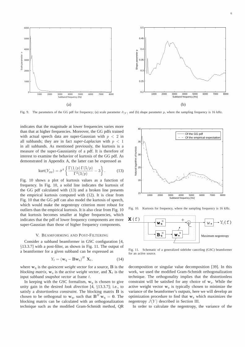
Subbands of speech can be precisely modeled by estimatingthe parameters of the GG pdf from training samples. From thetrained parameters, insight can be gained into the statisticalproperties of human speech. Fig. 9 shows the scale parameterσ|Y | and the shape parameterp calculated from the magnitudeof subband components plotted as functions of frequency,where the number of the subbands is 256. The training samplesused for estimating the GG pdf here were taken from cleanspeech data in the SSC2 development set [1].

It is clear from Fig. 9 that the scale parameterσ|Y | becomessmaller at higher frequencies. The scale parameterσ|Y | isrelated to the variance of|Y |, although not identical to it inthe case that the ML method is used in its estimation. Fig. 9

6

1000 2000 3000 4000 5000 6000 7000 80000

1000

2000

3000

4000

5000

6000

Subband frequency [Hz]

Sca

le p

ara

me

terσ

(a)

1000 2000 3000 4000 5000 6000 7000 80000.2

0.25

0.3

0.35

0.4

0.45

0.5

Subband frequency [Hz]

Sha

pe p

aram

eter

p

(b)

Fig. 9. The parameters of the GG pdf for frequency; (a) scale parameterσ|Y | and (b) shape parameterp, where the sampling frequency is 16 kHz.

indicates that the magnitude at lower frequencies varies morethan that at higher frequencies. Moreover, the GG pdfs trainedwith actual speech data are super-Gaussian withp < 2 inall subbands; they are in factsuper-Laplacianwith p < 1in all subbands. As mentioned previously, the kurtosis is ameasure of the super-Gaussianity of a pdf. It is therefore ofinterest to examine the behavior of kurtosis of the GG pdf. Asdemonstrated in Appendix A, the latter can be expressed as

kurt(Ygg) = σ4

{

Γ(1/p) Γ(5/p)

Γ2(3/p)− 3

}

. (13)

Fig. 10 shows a plot of kurtosis values as a function offrequency. In Fig. 10, a solid line indicates the kurtosis ofthe GG pdf calculated with (13) and a broken line presentsthe empirical kurtosis computed with (12). It is clear fromFig. 10 that the GG pdf can also model the kurtosis of speech,which would make the negentropy criterion more robust foroutliers than the empirical kurtosis. It is also clear from Fig. 10that kurtosis becomes smaller at higher frequencies, whichindicates that the pdf of lower frequency components are moresuper-Gaussian than those of higher frequency components.

V. BEAMFORMING AND POST-FILTERING

Consider a subband beamformer in GSC configuration [4,§13.3.7] with a post-filter, as shown in Fig. 11. The output ofa beamformer for a given subband can be expressed as

Yt = (wq − Bwa)H

Xt, (14)

wherewq is thequiescent weight vectorfor a source,B is theblocking matrix, wa is theactive weight vector, andXt is theinput subbandsnapshot vectorat framet.

In keeping with the GSC formalism,wq is chosen to giveunity gain in the desiredlook direction [4, §13.3.7]; i.e., tosatisfy adistortionless constraint. The blocking matrixB ischosen to be orthogonal towq, such thatBH

wq = 0. Theblocking matrix can be calculated with an orthogonalizationtechnique such as the modified Gram-Schmidt method, QR

1000 2000 3000 4000 5000 6000 7000 800015

20

25

30

35

40

Subband frequency [Hz]

Nat

ural

loga

rithm

of k

urto

sis

Of the GG pdfOf the empirical expectation

Fig. 10. Kurtosis for frequency, where the sampling frequency is 16 kHz.

w qH

B qH

X(f) +-+

Maximum negentropy

Y(f)w z

w aH

l

Fig. 11. Schematic of a generalized sidelobe canceling (GSC)beamformerfor an active source.

decomposition or singular value decomposition [39]. In thiswork, we used the modified Gram-Schmidt orthogonalizationtechnique. The orthogonality implies that the distortionlessconstraint will be satisfied for any choice ofwa. While theactive weight vectorwa is typically chosen to minimize thevariance of the beamformer’s outputs, here we will develop anoptimization procedure to find thatwa which maximizes thenegentropyJ(Y ) described in Section III.

In order to calculate the negentropy, the variance of the

7

beamformer outputsY is needed. Substituting (14) into thedefinition σ2

Y = E {Y Y ∗} of variance, we find

σ2Y = (wq − Bwa)

HΣX (wq − Bwa) , (15)

whereΣX = E{XXH} is the covariance matrix of the input

snapshot vectors.Maximizing the negentropy criterion yields a weight vector

wa capable of canceling interferences that leak through thesidelobes.

Zelinski post-filtering is performed on the output of thebeamformer. The transfer function of the Zelinski post-filtercan be expressed as

wz,t =

2M(M−1)

∣

∣

∣

∑M−1k=1

∑Ml=k+1 φkl,t

∣

∣

∣

1M

∑Mk=1 φkk,t

(16)

where φkk,t is the auto-spectral density of the time-alignedinput at microphonek and φkl,t is the cross-spectral density(CSD) at microphonek and l. The estimation of a desiredsignal can be improved by averaging the CSDs [26]. The finaloutput of the beamformer and post-filter combination is

Yl,t = wz,t Yt = wz,t (wq − Bwa)H

Xt. (17)

For the experiments described in Section VII, subband anal-ysis and synthesis were performed with a uniform DFT filterbank based on the modulation of a single prototype impulseresponse [40], which was designed to minimize each aliasingterm individually. Beamforming in the subband domain hasthe considerable advantage that the active sensor weights canbe optimized for each subband independently, which providesa tremendous computational saving with respect to a time-domain filter-and-sum beamformer with filters of the samelength on the output of each sensor.

In conventional beamforming,diagonal loading is oftenapplied in order to penalize large active weight vectors, andthereby improve robustness by inhibiting the formation ofexcessively large sidelobes [4,§13.3.8]. Such a regularizationterm can be applied in the present instance by defining themodified optimization criterion

J (Y ;α) = J(Y ) − α‖wa‖2 (18)

for some realα > 0.

A. Estimation of Active Weights under theΓ pdf

Here we describe the formulae necessary for estimating theactive weight vectors under theΓ pdf. Substituting (2) and (11)into (10), we can express the negentropy as

J(Y ) = log∣

∣σ2Y

∣

∣ + 2 (1 + log 2π) +1

T

T−1∑

t=0

log pY (Yt), (19)

where T is the number of frames used for weight vectoradaptation. We maximize the objective function which is thesum of the negentropy and the negative regularization term.Inthe absence of a closed-form solution for thewa maximizingthe negentropy (19), we resorted to theconjugate gradientsmethod [41,§1.6].

By substituting (19) into (18) and taking the partial deriva-tive on both sides, we obtain the gradient function,

∂J (Y ;α)

∂wa∗

=∂J(Y ;α)

∂wa∗

− αwa

=1

|σ2Y |

∂|σ2Y |

∂wa∗

+1

T

T−1∑

t=0

1

pY (Yt)

∂pY (Yt)

∂wa∗

− αwa

(20)

where

∂|σ2Y |

∂wa∗

=1

T

T−1∑

t=0

{

−BHXtY

∗t

}

. (21)

Equations (20) and (21) are sufficient to implement a nu-merical optimization algorithm, whereby the negentropyJ(Y )can be maximized. The details of the numerical optimizationalgorithm are described in Appendix B.

B. Estimation of Active Weights under the Generalized Gaus-sian pdf

1) Parameter optimization 1:Unlike the pdfs that can beexpressed as MeijerG-functions, the GG pdf cannot be readilyextended from the univariate to the multi-variate. Hence, weuse the magnitude of the beamformer’s output as the r.v. forcalculating the entropy. By substituting (5) and (11) into (10),we arrive at the following expression for negentropy

J(Y ) = log∣

∣σ2Y

∣

∣ + 2 (1 + log 2π) − HGG(|Y |). (22)

In order to apply the conjugate gradients algorithm, we mustonce more derive an expression for the gradient. By substi-tuting (22) into (18) and taking the partial derivative on bothsides while holding the shape parameter fixed, we obtain

∂J (Y ;α)

∂wa∗

=1

σ2Y

∂σ2Y

∂wa∗−

∂HGG(|Y |)

∂wa∗

− αwa, (23)

where

∂HGG(|Y |)

∂wa∗

=1

σ|Y |

∂σ|Y |

∂wa∗. (24)

Taking the derivative on both sides of (9), we find

∂σ|Y |

∂wa∗

=p

T

[

Γ(3/p)

Γ(1/p)

]12

×

[

p

T

T−1∑

t=0

|Yt|p

]

1p−1

×

[

T−1∑

t=0

|Yt|p−1 ∂|Yt|

∂wa∗

]

, (25)

where the gradient of the magnitude at each frame is

∂|Yt|

∂wa∗

= −1

2|Yt|B

HXtY

∗t . (26)

Based on (23) through (26), a numerical algorithm foroptimizing the active weight vector can be implemented. Thedetails of such an algorithm are given in Appendix B.

8

2) Parameter optimization 2:It is conceiveable that theentropy of the GG pdf for the complex valued r.v. could beapproximated by assuming that the real and imaginary partsare independent. Under such an assumption, the differentialentropy of the GG pdf can be expressed as

H(Y ) ≈ Hr(Yr) + Hi(Yi), (27)

whereYr is the real part ofY and Yi is its imaginary part.Notice that the shape parameters for the real and imaginaryparts must be trained individually.

Then, upon substituting (11) and (27) into (10) and addingthe regularization term, we obtain the objective function

J (Y ;α) = log∣

∣σ2Y

∣

∣ + 2 (1 + log 2π)

− Hr(Yr) − Hi(Yi) − α‖wa‖2.

(28)

In order to employ the gradient algorithm, we take thepartial derivative of (28)

∂J (Y ;α)

∂wa∗

=1

|σ2Y |

∂|σ2Y |

∂wa∗−

∂Hr(Yr)

∂wa∗

−∂Hi(Yi)

∂wa∗

− αwa

=1

|σ2Y |

∂|σ2Y |

∂wa∗−

1

σ|Yr|

∂σ|Yr|

∂wa∗−

1

σ|Yi |

∂σ|Yi |

∂wa∗− αwa.

(29)

We can readily calculateσ|Yr| and σ|Yi | in (29) based on (9).Each derivative can be obtained by replacing the magnitude|Yt| with an absolute value of the real part|Yr,t| or that of theimaginary part|Yi,t| in (25). The derivatives of the absolutevalues of the real and imaginary parts can be expressed,respectively, as

∂|Yr,t|

∂wa∗

= −1

2B

HXt · sign(Yr,t) (30)

and

∂|Yi,t|

∂wa∗

= j1

2B

HXt · sign(Yi,t). (31)

Equations (29) through (31) are used for the gradientalgorithm.

VI. SIMULATION

Conventional beamforming algorithms determine the op-timum weight vector that minimizes the variance of thebeamformer’s output,

wHΣXw, (32)

subject to the distortionless constraint in the look direction

wHd = 1, (33)

where d is the beam-steering vector. The well-known solu-tion is called the minimum variance distortionless response(MVDR) beamformer [4,§13.3.1]. The weight vector of theMVDR beamformer can be expressed as

wMVDR =Σ

−1X

d

dHΣ−1X

d. (34)

Additional weight is typically added to the main diagonalof ΣX in order to avoid excessively large sidelobes in the

beam pattern and the attendant nonrobustness [4,§13.3.7].The MVDR beamfomers would attempt to null out anyinterfering signal, but are prone to the signal cancellationproblem [5] whenever there is an interfering signal that iscorrelated with the desired signal. In realistic environments,interference signals are highly correlated with a target signalsince the target signal is reflected from hard surfaces suchas walls and tables. Therefore, the adaptation of the weightvector is usually halted whenever the desired source is active.Many techniques have been proposed in the literature toavoid signal cancellation. Perhaps the best-known of suchalgorithms is the robust beamformer in GSC configurationproposed by Hoshuyamaet al. [11]. In the lower branch,their algorithm adaptively estimates a blocking matrix whichcancels the signal correlated with the output from the upperbranch. Accordingly, the reflections of a desired signal canbe eliminated from the lower branch by the adaptive blockingmatrix (ABM). The coefficient of the ABM has upper andlower limits in order to specify the maximum allowable target-direction error. Then, the active weight vectors are estimatedso as to minimize the output of the beamformer. Since theABM can remove the reflections from the lower branch, thesignal cancellation problem is alleviated. However, the ABMcancels not only the reflections but also interference signalsin the case that the output of the upper branch contains theinterference components. In this case, their algorithm is unableto suppress the leaked interference signals. In reality, theinterference signals are often present in the upper branch dueto steering errors andspatial aliasing[4, §13.1.4]. Therefore,Hoshuyama’s algorithm requires in some sense a trade-offbetween the avoidance of signal cancellation and suppressionof the interference signals. This problem can be solved bysimply halting the adaptation of the ABM and only updatingthe active weight vectors in the case of a high signal-to-noiseratio (SNR) [13]. Such a switching algorithm is based on SNR,however, and requires complicated rules which must generallybe determined empirically.

Gannot et al. [8], [17], [18] proposed a transfer functionGSC (TF-GSC) which incorporates transfer functions fromthe desired source to microphones into the upper branch of theGSC. The ratios of the transfer functions from the source to themicrophone array are estimated with the least squares methodwhen the desired signal is present. The quiescent vectors arecalculated with the estimated ratios. The blocking matrices arethen computed so as to satisfy the orthogonality condition withthose quiescent weight vectors. Thus the leakage of the desiredsignal into the lower branch can be avoided. Their algorithmcan estimate the ratios of the transfer function without sourcepositions in acoustically stationary environments. It is diffi-cult, however, to obtain stable solutions under non-stationaryconditions. Although the algorithm proposed by Gannot et al.can be used in moderately reverberant environments, it doesnot reduce the amount of reverberation in the final signal [42].

E. Warsitz et al. proposed a generalized eigenvector (GEV)beamforming algorithm which constructs the blocking matrixbased on the maximum SNR criterion [15]. They first cal-culate beamformer weights which satisfy the maximum SNRcriterion. Secondly the orthogonal projection for constructing

9

reflection

source

30o

6m

70.9o 4m

6m

Fig. 12. Configuration of a source, sensors, and reflective surface forsimulation.

the blocking matrix is performed. Their algorithm estimatesthe transfer function from the source to the microphonesindirectly. They demonstrated that their method could reducesignal distortion and noise more than the TF-GSC withoutpost-filtering. It was also shown in [15] that their GEVbeamforming algorithm can achieve almost the same noisesuppression performance of the theoretical upper bound ob-tained by Hoshuyama’s beamformer.

Based on the solutions mentioned above that have appearedin the literature, it could be argued that conventional robustbeamforming algorithms have essentially addressed the prob-lem of removing reflections that are highly correlated withthe target signal in order to circumvent the signal cancellationproblem.

In contrast to such conventional beamformers, the MNbeamforming algorithm attempts not only to eliminate in-terference signals but alsostrengthenthose reflections fromthe desired source, assuming the desired sound source isstatistically independent of the other sources. Of course,anyreflected signal would be delayed with respect to the directpath signal. Such a delay would, however, manifest itself asa phase shift in the subband domain as long as it is shorterthan the length of an analysis filter, and could thus be removedthrough a suitable choice ofwa. Hence, the MN beamformeroffers the possibility of steering both nulls and sidelobes; theformer towards the undesired signal and its reflections, thelatter towards reflections of the desired signal.

In order to verify that the MN beamforming algorithm formssidelobes directed towards the reflection of a desired signal, weconducted experiments with a simulated acoustic environment.As shown in Fig. 12, we considered a simple configurationwith a sound source, a reflective surface, and a linear array ofeight microphones positioned with 10 cm inter-sensor spacing.Actual speech data were used as a source in this simulation,which was based on theimage method[43]. White Gaussiannoise was added to the output of each microphone to achievea SNR of 0 dB. We assumed that the speed of sound is 343.74meter per second and used a reflection coefficient of 0.7 forthe wall. Fig. 13 shows beam patterns atfs = 150 Hz, fs

= 650 Hz andfs = 1600 Hz obtained with a delay-and-sum (D&S) beamformer, the MVDR beamformer and the MNbeamforming algorithm with the GG pdf of the magnitude.The weights of the MVDR beamformer were optimized forisotropic (diffuse) noise in the simulation [44].

Given that a beam pattern shows the sensitivity of an

Fig. 15. The configuration of the meeting room (measurements in cm).

array to plane waves, but the beam patterns in Fig. 13 weremade with a near-field source and reflection, we also ran asecond set of simulations in which the source and reflectionwere assumed to produce plane waves. The results of thissecond simulation are shown in Fig. 14. It is clear from thesefigures that the MN beamformer emphasizes reflections fromthe desired source. The MVDR beamformer optimized forthe diffuse noise, on the other hand, tends to suppress suchreflections. It is also apparent from Fig. 13 (a) and Fig. 14 (a)that MVDR and MN beamformers can suppress interferenceat low frequencies, while the suppression performance of thedelay-and-sum beamformer is poor at low frequencies.

VII. E XPERIMENTS

We performed far-field automatic speech recognition (ASR)experiments on theMulti-Channel Wall Street Journal AudioVisual Corpus (MC-WSJ-AV) collected by theAugmentedMulti-party Interaction (AMI) project. The configuration ofthe meeting room is shown in Fig. 15; see Lincoln et al. [1]for the details of the data collection apparatus. The roomsize was 650 cm× 490 cm× 325 cm and the reverberationtime T60 was approximately 380 milliseconds. In addition tobeing reverberant, the meeting room data collected includesbackground noise from computers and the building ventilation.Some recordings also contain audible noise from outside themeeting room, such as that generated by passing cars andspeakers in an adjacent room.

The far-field speech data was recorded with a circular,eight-channel microphone array with a diameter of 20 cm.Additionally, a close-talking microphone was used for eachspeaker to capture the best possible signal as a reference.The sampling rate of the recordings was 16 kHz. As thedata was recorded with real speakers in a realistic acousticenvironment, the positions of the speakers’ heads as well asthespeaking volume varied even though the speakers were largelystationary. Indeed, it is exactly this behavior of real speakersthat makes working with data from corpora such as MC-WSJ-

10

−90 −70 −50 −30 −10 10 30 50 70 90−40

−30

−20

−10

0

10

20

target source

reflection

Direction of arrival [degree]

Nor

mal

ized

pow

er r

espo

nse

[dB

]

D & S BFMVDR BFMN BF with GG pdf(1)

(a)

−90 −70 −50 −30 −10 10 30 50 70 90−40

−30

−20

−10

0

10

20

target source

reflection

Direction of arrival [degree]

Nor

mal

ized

pow

er r

espo

nse

[dB

]

D & S BFMVDR BFMN BF with GG pdf(1)

(b)

−90 −70 −50 −30 −10 10 30 50 70 90−40

−30

−20

−10

0

10

20

target source

reflection

Direction of arrival [degree]

Nor

mal

ized

pow

er r

espo

nse

[dB

]

D & S BFMVDR BFMN BF with GG pdf(1)

(c)

Fig. 13. Beam patterns produced by a delay-and-sum beamformer, the MVDR beamformer and the MN beamforming algorithm using a spherical waveassumption for (a)fs = 150 Hz, (b)fs = 650 Hz and (c)fs = 1600 Hz.

−90 −70 −50 −30 −10 10 30 50 70 90−40

−30

−20

−10

0

10

20

target source reflection

Direction of arrival [degree]

Nor

mal

ized

pow

er r

espo

nse

[dB

]

D & S BFMVDR BFMN BF with GG pdf(1)

(a)

−90 −70 −50 −30 −10 10 30 50 70 90−40

−30

−20

−10

0

10

20

target source

reflection

Direction of arrival [degree]

Nor

mal

ized

pow

er r

espo

nse

[dB

]

D & S BFMVDR BFMN BF with GG pdf(1)

(b)

−90 −70 −50 −30 −10 10 30 50 70 90−40

−30

−20

−10

0

10

20

target source

reflection

Direction of arrival [degree]

Nor

mal

ized

pow

er r

espo

nse

[dB

]

D & S BFMVDR BFMN BF with GG pdf(1)

(c)

Fig. 14. Beam patterns produced by a delay-and-sum beamformer, the MVDR beamformer and the MN beamforming algorithm using a plane wave assumptionfor (a) fs = 150 Hz, (b)fs = 650 Hz and (c)fs = 1600 Hz.

AV so much more challenging than working with data thatwas played through a loudspeaker into a room, not to mentiondata that wasartificially convolvedwith previously-measuredimpulse responses. In thesingle speaker stationaryscenarioof the MC-WSJ-AV, a speaker was asked to read sentencesfrom six positions, four seated around the table in Seats 1-4shown in Fig. 15, one standing at the white board, and onestanding at the presentation screen.

The test set used for the experiments reported here containsrecordings of 10 speakers where each speaker reads approxi-mately 40 sentences taken from the 5,000 word vocabularyWall Street Journal (WSJ) task. This provided a total of352 utterances which correspond to 39.2 minutes of speech.There were a total of 11,598 word tokens in the referencetranscriptions. The test set was disjoint from the trainingdataset used to estimate the optimal scale and shape parameters.

As shown in [2] the directivity of the circular array atlow frequencies is poor; this stems from the fact that forlow frequencies, the wavelength is much longer than theaperture of the array. At high frequencies, the beam patternis characterized by very large sidelobes; this is due to the factthat at high frequencies, the spacing between the elements ofthe array exceeds half of a wavelength, thereby causing spatialaliasing [4,§13.1.4].

Prior to beamforming, we first estimated the speaker’sposition with a speaker tracking system [45]. Based on the av-erage speaker position estimated for each utterance, utterance-

dependent active weight vectorswa were estimated for asource. The active weight vectors for each subband wereinitialized to zero for estimation. Iterations of the conjugategradients algorithm were run on the entire utterance untilconvergence was achieved.

Zelinski post-filtering [26] was performed after beamform-ing. The feature extraction of our ASR system was based oncepstral features estimated with a warpedminimum variancedistortionless response[46] (MVDR) spectral envelope ofmodel order 30. Due to the properties of the warped MVDR,neither the Mel-filterbank nor any other filterbank was needed.The warped MVDR provides an increased resolution in low–frequency regions relative to the conventional Mel-filterbank.The MVDR also models spectral peaks more accurately thanspectral valleys, which leads to improved robustness in thepresence of noise. Front-end analysis involved extracting20cepstral coefficients per frame of speech and performing globalcepstral mean subtraction (CMS) with variance normalization.The final features were obtained by concatenating 15 con-secutive frames of cepstral features together, then performinga linear discriminant analysis(LDA) to obtain a featureof length 42. The LDA transformation was followed by asecond global CMS, then a global semi-tied covariance (STC)transform [47].

The far-field ASR experiments reported here were con-ducted with aword trace decoderimplemented along thelines suggested by Saonet al. [48]. The decoder is capable

11

of generating word lattices, which can then be optimizedwith weighted finite-state transducer (WFST) operations asin [49]; i.e., the raw lattice from the decoder is projectedonto the output side to discard all arc information save for theword identities, and then compacted through epsilon removal,determinization, and minimization [50].

We used 30 hours of American WSJ and the 12 hours ofCambridge WSJ data in order to train a triphone acousticmodel. The latter was necessary in order to provide coverageof the British accents for the speakers in the SSC developmentset [1]. Acoustic models estimated with two different HMMtraining schemes were used for the various decoding passes:conventional maximum likelihood (ML) HMM training [51,§12], and speaker-adapted training under a ML criterion (ML-SAT) [52]. Our baseline system was fully continuous with1,743 codebooks and a total of 67,860 Gaussian components.The parameters of the GG pdf were trained with 43.9 minutesof speech data recorded with the CTM in the SSC developmentset. The training data set for the GG pdf contains recordingsof 5 speakers.

We performed four decoding passes on the waveformsobtained with each of the beamforming algorithms describedin prior sections. Each pass of decoding used a differentacoustic model or speaker adaptation scheme. For all passessave the first unadapted pass, speaker adaptation parameterswere estimated using the word lattices generated during theprior pass, as in [53]. A description of the four decoding passesfollows:1. Decode with the unadapted, conventional ML acoustic

model.2. Estimate vocal tract length normalization (VTLN) [54]

parameters and constrained maximum likelihood linearregression parameters (CMLLR) [55] for each speaker, thenredecode with the conventional ML acoustic model.

3. Estimate VTLN, CMLLR, and maximum likelihood linearregression (MLLR) [56] parameters for each speaker, thenredecode with the conventional model.

4. Estimate VTLN, CMLLR, MLLR parameters for eachspeaker, then redecode with the ML-SAT model.

All passes used the full trigram LM for the 5,000 word WSJtask, which was made possible through the fast-on-the-flycomposition algorithm described in [57].

Table I shows the word error rates (WERs) for everybeamforming algorithm. As references, WERs in recognitionexperiments on speech data recorded with the single distantmicrophone (SDM) and CTM are also given. It is clear fromTable I that every MN beamforming algorithm can providebetter recognition performance than the simple delay-and-sumbeamformer (D&S BF) which can be improved by Zelinskipost-filtering (D&S BF with PF). It is also clear from Table Ithat MN beamforming with the GG pdf assumption which usesthe magnitude in calculating the negentropy (MN BF with GGpdf (1)) achieves the best recognition performance. This isdue to the fact that the GG pdf models the magnitudes of thesubband samples of speech better than the other pdfs in thatthe shape parameter for each subband is estimated individuallyfrom training data. The recognition performance, however,didnot improve for MN beamforming with the GG pdf when the

real and imaginary parts of the subband components wereassumed to be independent (MN BF with GG pdf (2)). Wefound it better to treat the subband components as spherically-invariant random processes (SIRPs) as in [2], [33] and are ledto conclude that the real and imaginary parts are dependent asmentioned in [25]. Table I suggests that theΓ pdf assumption(MN BF with Γ pdf) can lead to better noise suppressionperformance to some extent. The reduction over the D&S BFwith PF case, however, is limited because theΓ pdf cannotmodel the subband components of speech as precisely asthe GG pdf which takes the magnitude as the r.v. We alsoperformed recognition experiments on speech enhanced bythe MVDR beamformer with Zelinski post-filtering, which isequivalent to the minimum mean-squared error beamformer(MMSE BF) [4,§13.3.5]. Table I demonstrates that the MVDRbeamformer with post-filtering (MMSE BF) provides betterrecognition performance than D&S BF with PF. The MMSEbeamformer would suppress the reflections of the desiredsignal. On the other hand, as demonstrated in Section VI,the MN beamforming algorithm can strengthen the targetsignal by using the reflections solely based on the maximumnegentropy criterion. Note that the MVDR beamforming algo-rithms require speech activity detection in order to avoid signalcancellation. For the adaptation of the MVDR beamformer,we used the first 0.1 and last 0.1 seconds in each utterance,which contain only background noise. Table I also shows therecognition results obtained with the generalized eigenvectorbeamformer (GEV BF) proposed by E. Warsitz et al. [15].It achieved slightly better recognition performance than theMMSE beamformer. In this task, the transfer function fromthe sound source to the microphone array changes in time dueto movements of the speaker’s head. Moreover, it is difficulttodetermine whether or not the signal observed at any given timecontains both speech and noise components in each frequencybin, which are required to estimate the transfer function. Dueto these difficulties, the performance of the GEV beamformeris limited in realistic environments. Once more, in contrast toconventional beamforming methods, our algorithm does notneed to detect the start and end points of target speech sincetheproposed method can suppress noise and reverberation withoutthe signal cancellation problem. It is worth noting that thebestresult of 13.2% in Table I is significantly less than half theword error rate reported elsewhere in the literature on thisfar-field ASR task [1].

We also examined the effect of the regularization term inequation (18). Table II shows WER as a function of the regu-larization parameterα, where we used the MN beamformingalgorithm with the GG pdf of the magnitude r.v. We can seefrom the table that the regularization parameterα = 10−2

provided the lowest word error rate, although the impact ofdifferent values ofα on recognition performance was slight.The regularization parameterα could be interpreted as anindicator of the sufficiency of the input data in estimatingthe active weight vector. Thus, the requirement of a smallα may imply that the input data are not sufficiently reliableto completely determine the active weight vector due to, forexample, steering errors.

We implemented each beamforming algorithm in C/C++

12

TABLE I

WORD ERROR RATES FOR EACH BEAMFORMING ALGORITHM AFTER

EVERY DECODING PASS.

Beamforming Pass (%WER)Algorithm 1 2 3 4D&S BF 80.1 39.9 21.5 17.8

D&S BF with PF 79.0 38.1 20.2 16.5MMSE BF 78.6 35.4 18.8 14.8GEV BF 78.7 35.5 18.6 14.5

MN BF with Gamma pdf 75.6 34.9 19.8 15.8MN BF with GG pdf (1) 75.1 32.7 16.5 13.2MN BF with GG pdf (2) 79.0 37.2 20.0 16.7

SDM 87.0 57.1 32.8 28.0CTM 52.9 21.5 9.8 6.7

TABLE II

WORD ERROR RATES AGAINST THE REGULARIZATION PARAMETERα.

α Pass (%WER)1 2 3 4

α = 0.0 72.7 31.9 16.4 13.7α = 10

−3 73.9 32.2 16.6 13.6α = 10

−2 75.1 32.7 16.5 13.2α = 10

−1 76.2 32.5 17.5 13.5

and python. The computational cost of the MN beamformingalgorithm (MN BF with GG pdf (1)) is approximately 2.6times as much as that of the MMSE beamformer per frameon a machine with an Intel Core 2 DUO E6750/2.66GHzprocessor and 3.36 GB RAM.

VIII. C ONCLUSIONS ANDFUTURE WORK

In this work, we have proposed a novel beamformingalgorithm based on maximizing negentropy. Our first inves-tigations into the MN beamforming algorithm were basedon acoustic simulations. These simulations were sufficienttodemonstrate the MN beamforming algorithm could strengthenthe desired signal by constructively adding reflections of thesame. Moreover, the proposed method does not exhibit thesignal cancellation problems typically seen in conventionalbeamformers. We also evaluated theΓ and GG pdfs incalculating the negentropy through a set of far-field automaticspeech recognition experiments with data captured in realisticacoustic environments and spoken by real speakers. In theseexperiments, the MN beamforming algorithm with the GG pdfassumption proved to provide the best ASR performance.

We plan to develop an on–line version of the beamformingalgorithm presented here. This on–line algorithm will becapable of adjusting the active weight vectorswa,i with eachnew snapshot in order to track changes of speaker positionand movements of the speaker’s head during an utterance.

ACKNOWLEDGEMENT

We would like to thank Prof. Herve Bourlard for giving usthe opportunity to study about far-field speech recognition.

APPENDIX

A. Ther-th moment and kurtosis of the GG pdf

In this section, we derive two useful statistics of the GGpdf, ther-th moment and kurtosis.

The rth moment of the GG pdf can be expressed as

E {yr} =1

2Γ(1 + 1/p)A(p, σ)

∫ ∞

−∞

yr exp

[

−|y|

p

A(p, σ)

]

dy.

(35)Since the GG pdf is an even function about the mean, we canrewrite (35) as

E {yr} =1

Γ(1 + 1/p)A(p, σ)

∫ ∞

0

yr exp

[

−yp

Ap(p, σ)

]

dy. (36)

Upon defining

v =yp

Ap(p, σ),

from which it follows

dv

dy=

pyp−1

Ap(p, σ),

then (36) can be solved as

E {yr} =Ar(p, σ)

pΓ(1 + 1/p)

∫ ∞

0

vr+1

p−1 e−v dv

=Ar(p, σ)

pΓ(1 + 1/p)Γ

(

r + 1

p

)

. (37)

By substituting the second and fourth moments obtainedfrom Equation (37), the kurtosis of the GG pdf can now beexpressed as

kurt(Ygg) =A(p, σ)4

pΓ(1 + 1/p)Γ (5/p) − 3

{

A(p, σ)2

pΓ(1 + 1/p)Γ (3/p)

}2

. (38)

As pΓ(1 + 1/p) = Γ(1/p), Eqn. (38) can be simplified to

kurt(Ygg) = σ4

{

Γ(1/p) Γ(5/p)

Γ2(3/p)− 3

}

. (39)

B. The implementation of the optimization algorithm

Here we describe a nonlinear conjugate gradient methodfor our beamforming algorithm. Our goal is to find the activeweight vector which provides the maximum negentropy. How-ever, gradient algorithms are generally used to find the localminimum of a function [38,§1.6]. Accordingly, we explainhow to find the local minimum of the negative of (18) with aconjugate gradient algorithm, which is equivalent to seekingthe local maximum of (18).

The conjugate algorithms proceed as a succession of lineminimizations. The sequence ofconjugate directionsis usedto approximate the curvature of a cost function in the neigh-borhood of the minimum.

Expressing the objective function asI(wa∗) = −J (Y ;α),

we can calculate the initial search direction as that oppositeto the gradient according to

∆wa∗(0) = −

∂I(wa∗(0))

∂wa∗

,

where the required partial derivative is specified by oneof (20), (23) or (29). A line search is performed in thatdirection and a step size is optimized as follows:

β(0) := argminβ I(wa∗ + β∆wa

∗(0)) and

wa∗(1) = wa

∗(0) + β(0)∆wa

∗(0),

13

where the initial active weight vector is set to zero in thiswork.

After the first iteration, the following steps constitute oneiteration of searching the minimum along a subsequent con-jugate directionΛwa

∗(n), whereΛwa

∗(0) = ∆wa

∗(0) :

1. Calculate the gradient of the objective function

∆wa∗(n) = −

∂I(wa∗(n))

∂wa∗

.

2. Compute the modified Polak-Ribiere formula

γ(n) = Re

∆waT(n)

(

∆wa∗(n) − ∆wa

∗(n−1)

)

∆waT(n−1)∆wa

∗(n−1)

,

where(·)T denotes the transpose operation.3. Update the conjugate direction

Λwa∗(n) = ∆wa

∗(n) + γ(n)Λwa

∗(n−1).

4. Perform the line search and optimize the step size

β(n) = argminβ I(wa∗(n) + βΛwa

∗(n)). (40)

5. Update the estimate of the active weight vector

wa∗(n+1) = wa

∗(n) + β(n)Λwa

∗(n).

In each step, the line search is repeated until

Re{

∆wa(n) · Λwa∗(n)

}

< tol |∆wa(n)| |Λwa(n)|. (41)

where tol indicates the accuracy of the line search. We settol = 0.001 in our experiments. The convergence propertiesof the numerical search were not significantly altered bychanging the method used to calculateγ(n), nor by adjustingthe accuracy of the line search. Applying a more accuratemodel for the pdf of the subband samples of speech had alarger effect on the speed of convergence than any adjustmentof the parameters of the conjugate gradients search.

REFERENCES

[1] M. Lincoln, I. McCowan, I. Vepa, and H. K. Maganti, “The multi-channel Wall Street Journal audio visual corpus ( mc-wsj-av): Speci-fication and initial experiments,” inProc. IEEE workshop on AutomaticSpeech Recognition and Understanding (ASRU), 2005, pp. 357–362.

[2] K. Kumatani, T. Gehrig, U. Mayer, E. Stoimenov, J. McDonough, andM. Wolfel, “Adaptive beamforming with a minimum mutual informationcriterion,” IEEE Transactions on Audio, Speech and Language Process-ing, vol. 15, pp. 2527–2541, 2007.

[3] H. K. Maganti, D. Gatica-Perez, and I. McCowan, “Speech enhancementand recognition in meetings with an audio-visual sensor array,” IEEETransactions on Audio, Speech and Language Processing, vol. 15, pp.2257–2269, 2007.

[4] M. Wolfel and J. McDonough,Distant Speech Recognition. New York:Wiley, 2009.

[5] B. Widrow, K. M. Duvall, R. P. Gooch, and W. C. Newman, “Signalcancellation phenomena in adaptive antennas: Causes and cures,” IEEETransactions on Antennas and Propagation, vol. AP-30, pp. 469–478,1982.

[6] S. Nordholm, I. Claesson, and B. Bengtsson, “Adaptive array noisesuppression of handsfree speaker input in cars,”IEEE Transactions onVehicular Technology, vol. 42, pp. 514–518, 1993.

[7] W. Herbordt and W. Kellermann, “Adaptive beamforming for audiosignal acquisition,” inAdaptive Signal Processing: Applications to Real-World Problems, J. Benesty and Y. Huang, Eds. Berlin, Germany:Springer, 2003, pp. 155–194.

[8] I. Cohen, S. Gannot, and B. Berdugo, “An integrated real-time beam-forming and postfiltering system for nonstationary noise environments,”EURASIP Journal on Applied Signal Processing, vol. 2003, pp. 1064–1073, 2003.

[9] I. Claesson and S. Nordholm, “A spatial filtering approachto robustadaptive beaming,”IEEE Transactions on Antennas and Propagation,vol. 19, pp. 1093–1096, 1992.

[10] S. Nordebo, I. Claesson, and S. Nordholm, “Adaptive beamforming:spatial filter designed blocking matrix,”IEEE Journal of OceanicEngineering, vol. 19, pp. 583–590, 1994.

[11] O. Hoshuyama, A. Sugiyama, and A. Hirano, “A robust adaptive beam-former for microphone arrays with a blocking matrix using constrainedadaptive filters,”IEEE Transactions on Signal Processing, vol. 47, pp.2677–2684, 1999.

[12] N. Grbic, “Optimal and adaptive subband beamforming,” Ph.D. disser-tation, Blekinge Institute of Technology, 2001.

[13] W. Herbordt and W. Kellermann, “Frequency-domain integration ofacoustic echo cancellation and a generalized sidelobe canceller withimproved robustness,”European Transactions on Telecommunications(ETT), vol. 13, pp. 123–132, 2002.

[14] W. Herbordt, H. Buchner, S. Nakamura, and W. Kellermann, “Mul-tichannel bin-wise robust frequency-domain adaptive filtering and itsapplication to adaptive beamforming,”IEEE Transactions on Audio,Speech and Language Processing, vol. 15, pp. 1340–1351, 2007.

[15] E. Warsitz, A. Krueger, and R. Haeb-Umbach, “Speech enhancementwith a new generalized eigenvector blocking matrix for application in ageneralized sidelobe canceller,” inProc. IEEE International Conferenceon Acoustics, Speech, and Signal Processing (ICASSP), Las Vegas, NV,U.S.A, 2008.

[16] S. Doclo, A. Spriet, J. Wouters, and M. Moonen, “Frequency-domaincriterion for the speech distortion weighted multichannel wiener filterfor robust noise reduction,”Speech Communication, special issue onSpeech Enhancement, vol. 49, pp. 636–656, 2007.

[17] S. Gannot, David, Burshtein, and E. Weinstein, “Signalenhancementusing beamforming and nonstationarity with applications to speech,”IEEE Transactions on Signal Processing, vol. 49, pp. 1614–1626, 2001.

[18] S. Gannot and I. Cohen, “Speech enhancement based on the generaltransfer function GSC and postfiltering,”IEEE Transactions Speech andAudio Processing, vol. 12, pp. 561–571, 2004.

[19] S. Y. Low, S. Nordholm, and R. Togneri, “Convolutive blind signalseparation with post-processing,”IEEE Transactions on Speech andAudio Processing, vol. 12, pp. 539–548, 2004.

[20] H. Buchner, R. Aichner, and W. Kellermann, “Blind sourceseperationfor convolutive mixtures: A unified treatment,” inAudio Signal Process-ing for Next-Generation Multimedia Communication Systems, Y. Huangand J. Benesty, Eds. Boston: Kluwer Academic, 2004, pp. 255–289.

[21] H. Saruwatari, T. Kawamura, and K. Shikano, “Blind source separationbased on a fast-convergence algorithm combining ica and beamforming,”IEEE Transactions on Audio, Speech and Language Processing, vol. 14,pp. 666–678, 2006.

[22] P. Smaragdis, “Efficient blind separation of convolved sound mixtures,”in IEEE ASSP Workshop on Applications of Signal Processing to Audioand Acoustics, New Paltz, NY, U.S.A, 1997.

[23] L. C. Parra and C. V. Alvino, “Geometric source separation: Merg-ing convolutive source separation with geometric beamforming,” IEEETransactions Speech Audio Processing, vol. 10, no. 6, pp. 352–362,September 2002.

[24] R. Martin, “Speech enhancement based on minimum mean-square errorestimation and supergaussian priors,”IEEE Transactions Speech andAudio Processing, vol. 13, no. 5, pp. 845–856, Sept. 2005.

[25] J. S. Erkelens, R. C. Hendriks, R. Heusdens, and J. Jensen, “Mini-mum mean-square error estimation of discrete fourier coefficients withgeneralized gamma priors,”IEEE Transactions on Audio, Speech andLanguage Processing, vol. 15, pp. 1741–1752, 2007.

[26] C. Marro, Y. Mahieux, and K. U. Simmer, “Analysis of noise reductionand dereverberation techniques based on microphone arrays with post-filtering,” IEEE Transactions on Speech and Audio Processing, vol. 6,pp. 240–259, 1998.

[27] I. A. McCowan and H. Bourlard, “Microphone array post-filter basedon noise field coherence,”IEEE Transactions on Speech and AudioProcessing, vol. 11, pp. 709–716, 2003.

[28] S. Leukimmiatis, D. Dimitriadis, and P. Maragos, “An optimum mi-crophone array post-filter for speech application,” inProc. Interspeech-ICSLP, Pittsburgh, PA, U.S.A, 2006.

[29] H. Yoon and H. Ko, “Microphone array post-filter using inputoutput ratioof beamformer noise power spectrum,”Electronics Letters, vol. 43, pp.1003–1005, 2007.

14

[30] A. Hyvarinen and E. Oja, “Independent component analysis: Algorithmsand applications,”Neural Networks, 2000.

[31] R. G. Gallager,Information Theory and Reliable Communication. NewYork: John Wiley & Sons, 1968.

[32] F. D. Neeser and J. L. Massey, “Proper complex random processes withapplications to information theory,”IEEE Transactions Info. Theory,vol. 39, no. 4, pp. 1293–1302, July 1993.

[33] H. Brehm and W. Stammler, “Description and generation of sphericallyinvariant speech-model signals,”Signal Processing, vol. 12, pp. 119–141, 1987.

[34] S. Wolfram,The Mathematica Book, 3rd ed. Cambridge: CambridgeUniversity Press, 1996.

[35] K. Kokkinakis and A. K. Nandi, “Exponent parameter estimation forgeneralized gaussian probability density functions with application tospeech modeling,”Signal Processing, vol. 85, pp. 1852–1858, 2005.

[36] M. K. Varanasi and B. Aazhang, “Parametric generalized gaussiandensity estimation,”J. Acoust. Soc. Am., vol. 86, pp. 1404–1415, 1989.

[37] M. K. Varanasi, “Parameter estimation for the generalized gaussian noisemodel,” Ph.D. dissertation, Rice University, 1987.

[38] D. P. Bertsekas,Nonlinear Programming. Belmont, Massachusetts:Athena Scientific, 1995.

[39] G. H. Golub and C. F. Van Loan,Matrix Computations, 3rd ed.Baltimore: The Johns Hopkins University Press, 1996.

[40] K. Kumatani, J. McDonough, S. Schacht, D. Klakow, P. N. Garner, andW. Li, “Filter bank design based on minimization of individualaliasingterms for minimum mutual information subband adaptive beamforming,”in Proc. IEEE International Conference on Acoustics, Speech,andSignal Processing (ICASSP), Las Vegas, Nevada, U.S.A, 2008.

[41] D. P. Bertsekas,Nonlinear Programming. Belmont, MA, USA: AthenaScientific, 1995.

[42] E. A. P. Habets, “Single- and multi microphone speech dereverberationusing spectral enhancement,” Ph.D. dissertation, Eindhoven Universityof Technology, 2007.

[43] J. B. Allen and D. A. Berkley, “Image method for efficientlysimulatingsmall-room acou stics,”J. Acoust. Soc. Am., vol. 65, no. 4, pp. 943–950,April 1979.

[44] M. Brandstein and D. Ward, Eds.,Microphone Arrays. Heidelberg,Germany: Springer Verlag, 2001.

[45] T. Gehrig, U. Klee, J. McDonough, S. Ikbal, M. Wolfel, and C. Fugen,“Tracking and beamforming for multiple simultaneous speakers withprobabilistic data association filters,” inProc. Interspeech, 2006, pp.2594–2597.

[46] M. Wolfel and J. McDonough, “Minimum variance distortionless re-sponse spectral estimation: Review and refinements,”IEEE SignalProcessing Magazine, vol. 22, no. 5, pp. 117–126, Sept. 2005.

[47] M. J. F. Gales, “Semi-tied covariance matrices for hiddenMarkovmodels,” IEEE Transactions Speech and Audio Processing, vol. 7, pp.272–281, 1999.

[48] G. Saon, D. Povey, and G. Zweig, “Anatomy of an extremely fastLVCSR decoder,” inProc. Interspeech, Lisbon, Portugal, 2005, pp. 549–552.

[49] A. Ljolje, F. Pereira, and M. Riley, “Efficient general lattice generationand rescoring,” inProc. Eurospeech, Budapest, Hungary, 1999, pp.1251–1254.

[50] M. Mohri and M. Riley, “Network optimizations for large vocabularyspeech recognition,”Speech Communication, vol. 28, no. 1, pp. 1–12,1999.

[51] J. Deller, J. Hansen, and J. Proakis,Discrete-Time Processing of SpeechSignals. New York: Macmillan Publishing, 1993.

[52] T. Anastasakos, J. McDonough, R. Schwarz, and J. Makhoul, “Acompact model for speaker-adaptive training,” inProc. ICSLP, 1996,pp. 1137–1140.

[53] L. Uebel and P. Woodland, “Improvements in linear transform basedspeaker adaptation,” inProc. IEEE International Conference on Acous-tics, Speech, and Signal Processing (ICASSP), 2001.

[54] L. Welling, H. Ney, and S. Kanthak, “Speaker adaptive modeling byvocal tract normalization,”IEEE Transactions on Speech and AudioProcessing, vol. 10, no. 6, pp. 415–426, 2002.

[55] M. J. F. Gales, “Maximum likelihood linear transformations for HMM-based speech recognition,”Computer Speech and Language, vol. 12,1998.

[56] C. J. Leggetter and P. C. Woodland, “Maximum likelihood linearregression for speaker adaptation of continuous density hidden markovmodels,” Computer Speech and Language, vol. 9, pp. 171–185, April1995.

[57] J. McDonough, E. Stoimenov, and D. Klakow, “An algorithmforfast composition of weighted finite-state transducers,” inProc. IEEEworkshop on Automatic Speech Recognition and Understanding (ASRU),2007.