December 2006

NASA/CR-2006-214529

Bearing-Load Modeling and Analysis Study for Mechanically Connected Structures Norman F. Knight, Jr. General Dynamics – Advanced Information Systems, Chantilly, Virginia

https://ntrs.nasa.gov/search.jsp?R=20070003749 2018-05-02T05:07:10+00:00Z

The NASA STI Program Office . . . in Profile

Since its founding, NASA has been dedicated to the advancement of aeronautics and space science. The NASA Scientific and Technical Information (STI) Program Office plays a key part in helping NASA maintain this important role.

The NASA STI Program Office is operated by Langley Research Center, the lead center for NASA’s scientific and technical information. The NASA STI Program Office provides access to the NASA STI Database, the largest collection of aeronautical and space science STI in the world. The Program Office is also NASA’s institutional mechanism for disseminating the results of its research and development activities. These results are published by NASA in the NASA STI Report Series, which includes the following report types:

• TECHNICAL PUBLICATION. Reports of

completed research or a major significant phase of research that present the results of NASA programs and include extensive data or theoretical analysis. Includes compilations of significant scientific and technical data and information deemed to be of continuing reference value. NASA counterpart of peer-reviewed formal professional papers, but having less stringent limitations on manuscript length and extent of graphic presentations.

• TECHNICAL MEMORANDUM. Scientific

and technical findings that are preliminary or of specialized interest, e.g., quick release reports, working papers, and bibliographies that contain minimal annotation. Does not contain extensive analysis.

• CONTRACTOR REPORT. Scientific and

technical findings by NASA-sponsored contractors and grantees.

• CONFERENCE PUBLICATION. Collected

papers from scientific and technical conferences, symposia, seminars, or other meetings sponsored or co-sponsored by NASA.

• SPECIAL PUBLICATION. Scientific,

technical, or historical information from NASA programs, projects, and missions, often concerned with subjects having substantial public interest.

• TECHNICAL TRANSLATION. English-

language translations of foreign scientific and technical material pertinent to NASA’s mission.

Specialized services that complement the STI Program Office’s diverse offerings include creating custom thesauri, building customized databases, organizing and publishing research results ... even providing videos. For more information about the NASA STI Program Office, see the following: • Access the NASA STI Program Home Page at

http://www.sti.nasa.gov • E-mail your question via the Internet to

help@sti.nasa.gov • Fax your question to the NASA STI Help Desk

at (301) 621-0134 • Phone the NASA STI Help Desk at

(301) 621-0390 • Write to:

NASA STI Help Desk NASA Center for AeroSpace Information 7115 Standard Drive Hanover, MD 21076-1320

National Aeronautics and Space Administration Langley Research Center Prepared for Langley Research Center Hampton, Virginia 23681-2199 under NASA Order No. NNL05AD09D

December 2006

NASA/CR-2006-214529

Bearing-Load Modeling and Analysis Study for Mechanically Connected Structures Norman F. Knight, Jr. General Dynamics – Advanced Information Systems, Chantilly, Virginia

Available from: NASA Center for AeroSpace Information (CASI) National Technical Information Service (NTIS) 7115 Standard Drive 5285 Port Royal Road Hanover, MD 21076-1320 Springfield, VA 22161-2171 (301) 621-0390 (703) 605-6000

Trade names and trademarks are used in this report for identification only. Their usage does not constitute an official endorsement, either expressed or implied, by the National Aeronautics and Space Administration.

1

Bearing-Load Modeling and Analysis Study for Mechanically Connected Structures

Norman F. Knight, Jr.

General Dynamics – Advanced Information Systems Chantilly, VA

Abstract Bearing-load response for a pin-loaded hole is studied within the context of two-dimensional finite element analyses. Pin-loaded-hole configurations are representative of mechanically connected structures, such as a stiffener fastened to a rib of an isogrid panel, that are idealized as part of a larger structural component. Within this context, the larger structural component may be idealized as a two-dimensional shell finite element model to identify load paths and high stress regions. Fastener modeling within these analysis models is often of low fidelity and limitations need to be assessed. Finite element modeling and analysis aspects of a pin-loaded hole are considered in the present paper including the use of linear and nonlinear springs to simulate the pin-bearing contact condition. For a repeating unit of a square domain with a center circular hole, the effects of hole diameter and degree of elastic restraint provided by material surrounding the hole are considered. These effects are found to affect the local response by changing it from a bearing-dominated response for small holes to a plane-stress-dominated ligament response for larger holes. For a T-shaped coupon specimen configuration, the pin-loaded-hole case resulted in higher local stresses around the hole, while the open-hole case generated high stresses along the majority of the free edge of the T-specimen web. Simulating pin-connected structures within a two-dimensional finite element analysis model using nonlinear spring or gap elements provides an effective way for accurate prediction of the local effective stress state and peak forces.

Introduction Mechanically connected structures using fasteners and bolted/pinned joints are a common occurrence in most engineering designs. Design procedures for bolted joints have been developed (e.g., Bickford [1]) and generally lead to successful applications and safe structures. However, in some extreme cases, failure investigations have found that some failures are attributed to local material failures in the vicinity of mechanical connections. Detailed local three-dimensional finite element analyses including contact and material nonlinearities of the connection are typically used in failure investigations of such cases. However, in the global analysis of the overall structure, various modeling assumptions are employed to simulate the mechanical connections.

Modeling and analysis of mechanically connected structures using fasteners and bolted/pinned joints continue to challenge stress analysts. While commercial finite element analysis tools offer a wide range of contact modeling options for three-dimensional simulations, fastener modeling and bearing-load simulations within a two-dimensional shell finite element analysis model requires care in idealization of the connection and local finite element discretization. Understanding is needed of the local load distribution as a combination of bearing load and net-

2

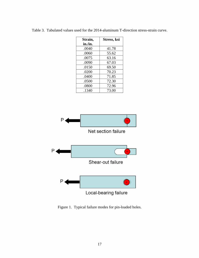
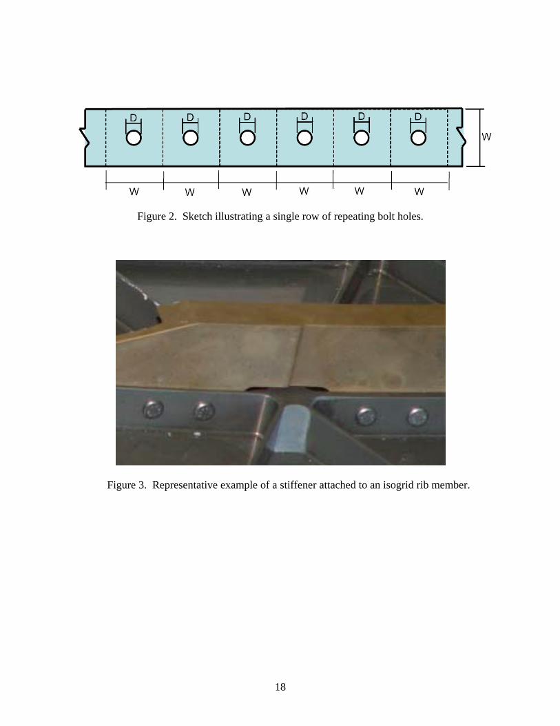
section load and of any load redistribution effects to the surrounding structure. Typically, the loading is defined as a bearing-to-bypass load ratio (e.g., see Refs. 2 and 3). The bearing load may result in a net-section failure, a shear-out failure, or local bearing failure due to plastic deformations as indicated in Figure 1. For simple geometries and loading conditions, a bolted joint can be readily examined. Engineering design solutions used in tandem with large safety factors account for uncertainties associated with the bolted joint itself. For complex geometries and/or loading conditions, the weak link in a design is frequently associated with a fastener connection due in part to uncertainties in manufacturing tolerances and assembly variability. Often a series of fasteners as illustrated in Figure 2 are commonly used to attach separate structural components together or to attach independent stiffener elements to other integrally stiffened panel components. One such application is the augmentation of an existing integrally stiffened structural design by attaching a local stiffener to the rib of isogrid panel as shown in Figure 3. This type of design augmentation may be needed to account for changes in design loads versus actual loads or to account for changes needed to extend performance limits and should be thoroughly assessed prior to implementation.

Modeling and analysis of a bearing-load problem poses several challenges. First, modeling of the bearing-load distribution around the bearing surface (i.e., pin-loaded hole) can be idealized in several ways: through the use of rigid constraints; through the use of springs; and through the use of explicit body-to-body contact simulation. Second, the bearing response often corresponds to the formation of a local plastic zone in the region of the bearing-contact response, which requires an elastic-plastic analysis. Third, redistribution of the bearing load occurs as plasticity develops requiring sufficient finite element modeling fidelity to capture the load redistribution and the localized stress gradient. Fourth, elongation of the pin-loaded hole can result in bearing loads on the sides of the pin resulting from local deformations near the hole. A pin-bearing behavior can be observed due the applied loading plus a side pinching bearing load due to hole geometry changes. These challenges are addressed in different ways depending on the objectives of the overall structural analysis. Often global finite element models of a complete structural assembly are created to identify overall load paths and regions of high stress. Such finite element models are usually two-dimensional shell finite element models having rather limited spatial discretization in the vicinity of stress concentrations. Global/local modeling methodologies can be used to examine local response behavior using a high-fidelity local model for the bearing response and a lower fidelity global model to establish load paths. The local model could involve a three-dimensional finite element representation of both the connected parts as well as the connector (pin or bolt) wherein explicit body-to-body contact is simulated for the assembly. Most commercial finite element analysis tools include a capability to simulate three-dimensional body-to-body contact through nonlinear analysis. These local analyses, however, are dependent on the global modeling to capture the basic structural response characteristics along the interface between the global and local regions. The present paper addresses the global two-dimensional finite element modeling and analysis needs for a representative mechanical connection.

Numerical studies are performed to investigate the bearing-load response for a thin structural member with a hole subjected to pin-bearing load. Different aspects of the bearing-load problem are examined including the effect of hole-diameter-to-plate-width (D/W) ratio, the effect of edge boundary conditions, the effect of mesh refinement, and the effect of pin-bearing idealization. Verification simulations using a square domain with a center circular hole as a repeating unit are performed to understand the finite element modeling aspects of the pin-loaded-hole response. Coupon-level simulations of a two-hole T-section test configuration described by Newman et al.

3

[4] are also performed to investigate the effect of pin-bearing behavior in a more complex configuration. The T-section configuration is related to an integrally stiffened isogrid structure with holes in a rib of the isogrid stiffener that are loaded by pin-bearing forces.

An outline of the present paper is as follows. First, a brief description of the analysis tool and the computational environment is presented. Then, the verification analysis effort using a simple repeating unit is described. Application of these findings to a T-shaped coupon are then applied and summarized. The present paper concludes with concluding remarks and references.

Analysis Tool and Computational Environment The finite element analyses are performed using the STAGS nonlinear finite element tool [5, 6]. STAGS (STructural Analysis of General Shells) has a variety of finite elements to use in modeling structures as well as material models for elastic, elasto-plastic, and composite material systems. The STAGS E410 4-node shell finite element [7] is used for the present analyses. The E410 element has six degrees of freedom per node where the drilling freedom contributes to the in-plane displacement field approximations. The membrane and bending approximations are superimposed within the element formulation allowing it to be used as a plane-stress element, a plate-bending element, or a shell element with combined plane-stress and bending behavior. The E410 shell element is considered to be the STAGS “workhorse” element.

Both geometric (large-displacements and large rotations) and material (elastic-plastic) nonlinearities are treated by STAGS. Geometric nonlinearities are handled through the use of the Green-Lagrange nonlinear strain-displacement relations and the element-independent co-rotational formulation [8]. STAGS has some contact modeling capability and in addition has nonlinear spring or gap elements, called MOUNT elements, that can be used to simulate pin-bearing behavior [5].

Material nonlinearities, which are in the form of an elastic-plastic stress-strain curve, are handled through the use of a White-Besseling or mechanical sublayer plasticity model [9-14]. Bushnell [12] described the White-Besseling model for strain-hardening materials that exhibit a Bauschinger effect as “an amalgam of separate elastic-perfectly plastic” sublayers. Each sublayer is subject to the same total strain but may have different elastic limits. With one sublayer, the material behaves as elastic-perfectly plastic. With two sublayers, the material behaves as a material with a bilinear stress-strain curve and kinematic strain hardening. With multiple sublayers, the stress-strain curve is approximated by a series of piecewise linear segments.

The nonlinear solution procedure is an incremental-iterative solution procedure. Nonlinear solution procedure options include the form of the Newton-Raphson approach (full or modified approach), the type of solution control (load-control, displacement control or arc-length control), and the convergence criterion (norm of the incremental change in displacements, norm of the equilibrium force imbalance, or normalized work-done by the force imbalance). Historically, STAGS has been used to solve many stiffened and unstiffened shell analysis problems including structures with cutouts.

The computational environment for the finite element modeling, analysis, and post-processing is a high-end multiple-CPU personal computer running SUSE1 Linux Enterprise Server v9.0. 1 SUSE is a trademark of Novell, Inc.

4

However, STAGS is not configured to exploit multiple processors. The computational platform, named “chameleon”, has four 2.0-GHz AMD Opteron2 846 processors with a total of 16 gigabytes of shared memory. The computing system includes two 146-gigabyte internal SCSI disk drives that are used for the operating system and a 4-terabyte external SATA RAID that is used for user directories and computational scratch (temporary) disk space.

Numerical Results and Discussion Two sets of computations are summarized in this section. First, a verification bearing-response problem based on a repeating unit is examined. The repeating unit is a square domain of uniform thickness with a central circular hole. Parametric studies using two-dimensional plane-stress analysis models are performed to investigate how the bearing response is influenced by hole diameter, spatial discretization, edge boundary conditions, pin-bearing simulation, and unit force line of action. Then, having established a basis for the finite element modeling using two-dimensional shell finite elements and nonlinear spring elements, a T-shaped coupon-level structural problem with a pin-loaded hole is analyzed.

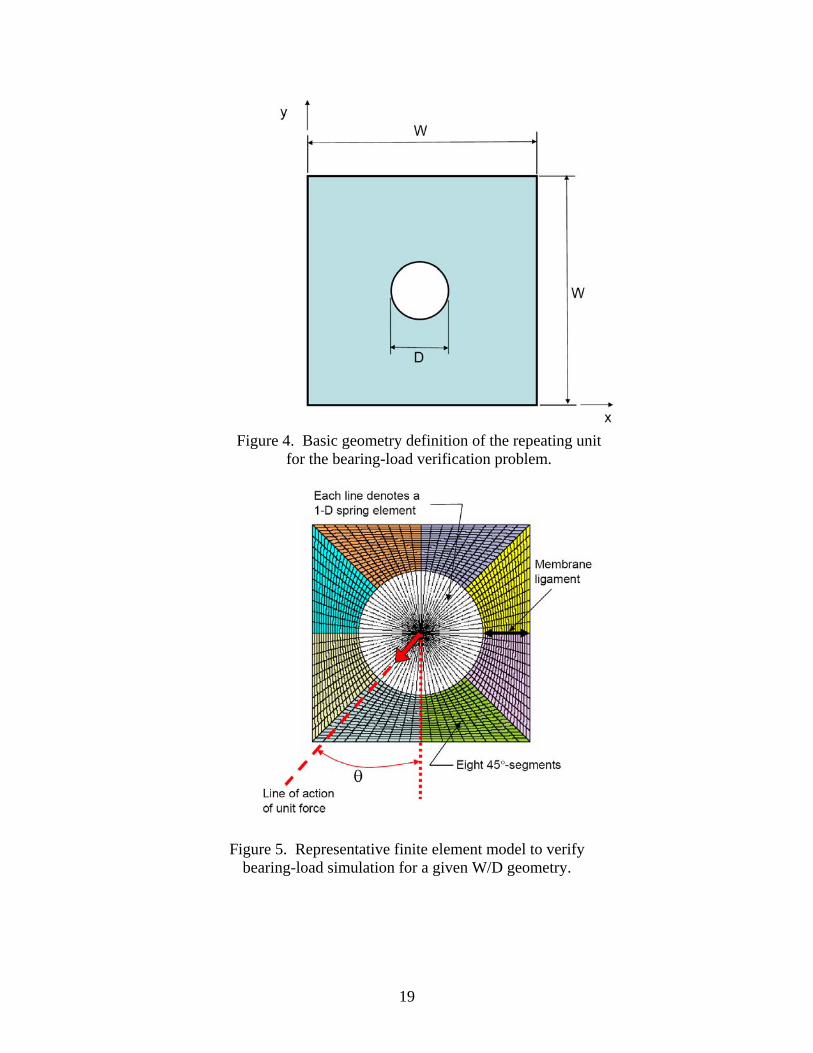
Verification Modeling and Analysis of Repeating Unit Verification modeling and analysis are performed using a repeating unit from Figure 2 – a square domain with side lengths equal to W with a central, circular hole of diameter D as shown in Figure 4. The domain has a uniform thickness of 0.105 inches. The nominal hole diameter D0 is 0.252 inches, and the nominal width W is 0.88 inches. The material is 2014 aluminum with an elastic modulus of 10.44 Msi, a Poisson’s ratio of 0.33, and a yield strength of 66,000 psi. The present problem is a two-dimensional plane-stress problem modeled using shell finite elements. The out-of-plane deformation state (in terms of the w, RX, RY degrees of freedom3) is computed to be zero for the loading case considered. The use of shell elements (with nodes having all six degrees of freedom) rather than plane-stress elements (with nodes have only two degrees of freedom: u and v and possibly RZ for elements with “drilling” degrees of freedom) is a matter of convenience here and for consistency with the follow-on problem that does exhibit out-of-plane deformations.

The square domain is divided into eight 45° segments around a central circular hole for generating the finite element meshes. These eight regions are denoted by different colors in Figure 5. A finite element mesh is defined in terms of the number of “spokes” of 4-node quadrilateral elements around the hole and the number of “rings” of 4-node quadrilateral elements across the plane-stress ligaments. The most refined finite element mesh of the repeating unit considered in the present study is shown in Figure 5. The finite element model of each 45° segment has ten “spokes” of 4-node quadrilateral elements around the hole (4.5° per element) and twenty “rings” of 4-node quadrilateral elements radially outward from the edge of the hole across a plane-stress ligament. The finite element model shown in Figure 5 involves 1,930 nodes, 80 spring elements, and 1,600 4-node quadrilateral finite elements.

2 AMD Opteron is a trademark of Advanced Micro Devices, Inc. 3 The notations u, v, and w refer to the translational degrees of freedom along the x-, y-, and z-axes, respectively. The notations RX, RY, and RZ refer to the rotational degrees of freedom about the x-, y-, and z-axes, respectively. w, RX, and RY relate to out-of-plane bending behavior. RZ relates to in-plane plane-stress behavior for some two-dimensional elements with “drilling” degrees of freedom.

5

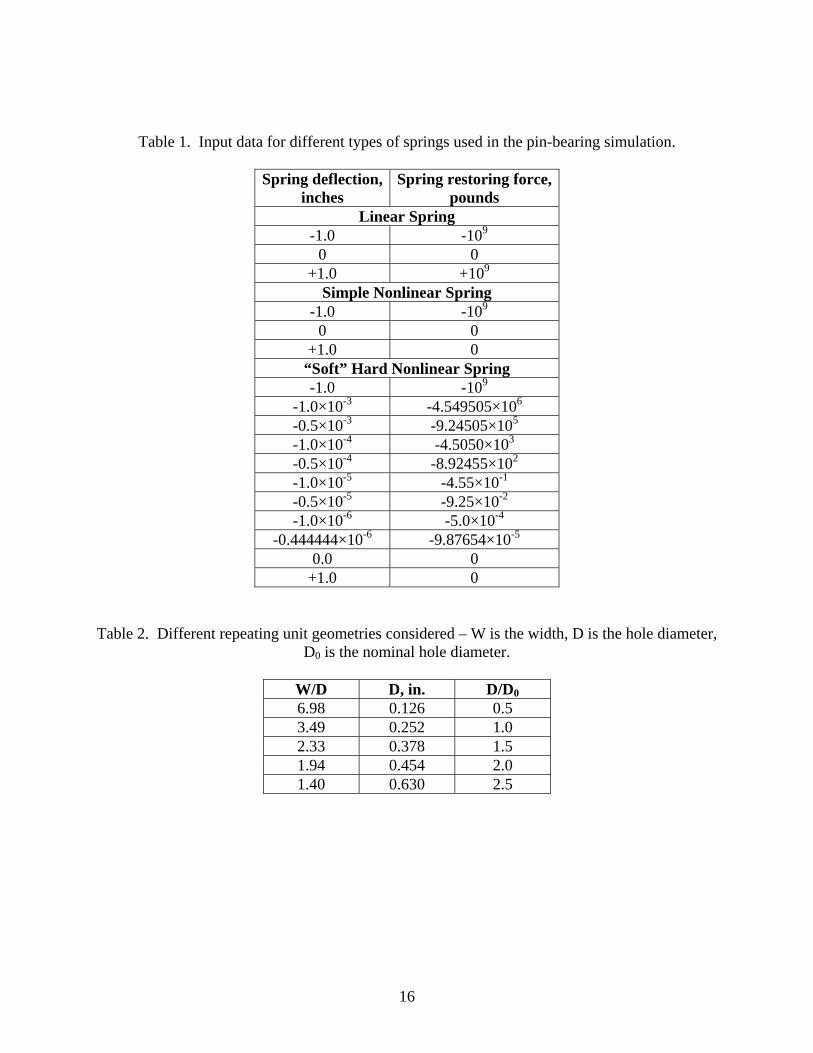
Pin-bearing response in this two-dimensional analysis model is simulated through a series of one-dimensional spring elements emanating from the center of the hole – one for each node on the edge of the hole and connected to the pin center as indicated in Figure 5. Linear spring elements have the same constant stiffness whether stretched or compressed as indicated in Table 1. Nonlinear spring elements require a user-defined force-deflection curve. Often a simple nonlinear spring force-deflection response is prescribed as indicated in Table 1; however, such a definition can potentially cause numerical convergence problems for the nonlinear solution procedure due to the abrupt change in stiffness. To alleviate this issue, an alternate nonlinear spring force-deflection response, also indicated in Table 1, can be used. This alternate approach has been referred to as a “soft” hard spring4 and is based on assuming a piecewise linear distribution for the spring stiffness and integrating over the spring deflection to obtain the required force. For the present analyses, the second approach is employed. For the present studies, the nonlinear spring elements, called MOUNT elements in STAGS, have essentially infinite stiffness if compressed, and near-zero stiffness if extended. Hence, they represent a simple way of modeling nonlinear contact for pin-loaded holes without requiring explicit body-to-body contact modeling and without requiring explicit finite element modeling of the pin. This idealization assumes that the pin is rigid and pin deformations are ignored, and therefore failure modes associated with the pin cannot be represented or simulated by this approach. However, this modeling approach does provide a computationally attractive approach for bearing-contact simulation.

The applied load is defined as a unit force acting at the pin center with its line of action defined by the angle θ as measured from the vertical axis in a clockwise direction (see Figure 5). As the direction of the unit force changes (by varying the angle θ), the bearing-contact location on the hole boundary also changes. However, the bearing region always remains within a 180°-arc (θ±90°) along the hole boundary for a nonlinear spring model rather than along the entire hole boundary as in a linear spring model. The magnitude of the applied force directed radially outward from the pin center is a unit force (i.e., one pound). For the unit-force case, the material response remains elastic. The bearing response is characterized qualitatively using contour plots of the effective stress distribution where the effective (or von Mises) stress for a plane-stress problem is given by

( ) 2222 62

1xyyxyxeff τσσσσσ +++−= (1)

The effective stress is a scalar quantity and readily indicates an overall stress level for isotropic ductile materials by comparing its value to the material’s yield stress. However, in the verification problems with only a unit force applied, local material yielding is not anticipated (i.e., the effective stress is anticipated to be well below the 66,000-psi yield stress value).

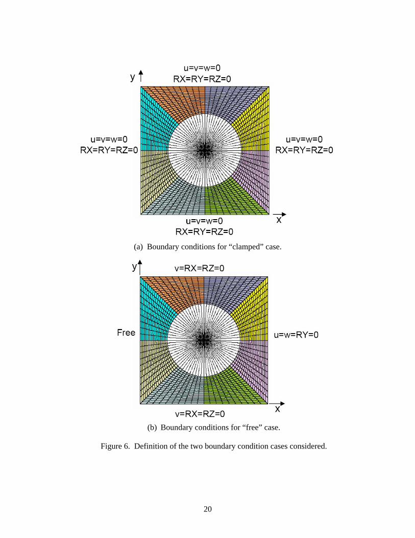
Two sets of boundary conditions along the straight sides of the square domain are considered as indicated in Figure 6. The first set, referred to as the “clamped” set and shown in Figure 6a, corresponds to having all outside straight edges of the domain clamped (fully restrained). In so doing, the applied force should be reacted in a similar way regardless of which quadrant the unit force at the center of the pin is directed since the domain is equally restrained in all quadrants.

4 The “soft” hard spring approach is attributed to Dr. Charles Rankin of Rhombus Consulting Group, Inc., Palo Alto, CA. A few values are defined and the remaining values are then obtained by interpolation.

6

The second set, referred to as the “free” set and shown in Figure 6b, corresponds to a set of boundary conditions that would be evident in a larger stiffened structure simulating a stiffener attachment to another structural member such as a rib in an isogrid panel (e.g., like the component shown in Figure 2). In this case, one edge (along x=0 in Figure 4) is free, the opposite edge (along x=W) has boundary conditions given by u=w=RY=0, and the remaining edges (along y=0 and y=W) have symmetry boundary conditions (v=RX=RZ=0).

Four parametric studies are performed. The first study focuses on finite element mesh convergence for the pin-bearing problem. The second study focuses on the pin-bearing modeling for two-dimensional analysis models using spring elements. The third study focuses on the effect of different hole diameters for a fixed domain width (W=0.88 inches) on the bearing response. The fourth study focuses on the effect of two different sets of boundary conditions along the outer edges of the square domain on the bearing response. All simulations account for both geometric and material nonlinearities even though an elastic, small deformation structural response is anticipated for the unit load – a nonlinear analysis is required for the nonlinear spring model in any event.

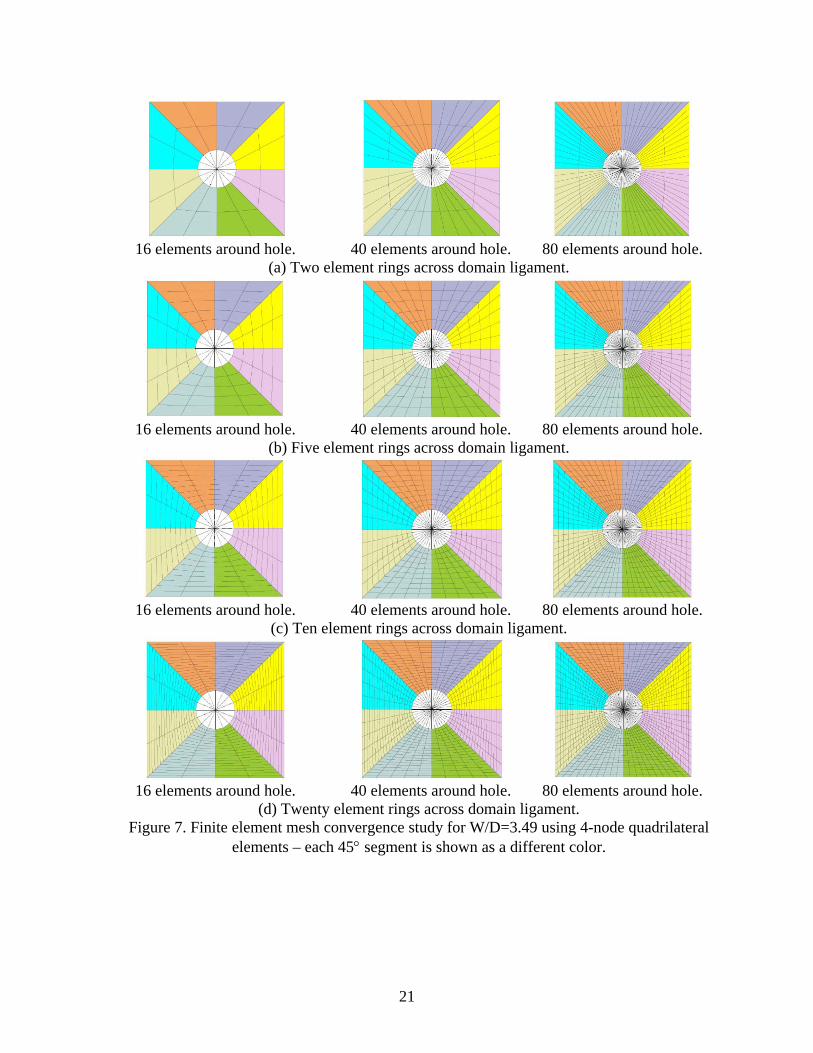
Effect of Spatial Discretization A finite element mesh convergence study is performed first using the finite element models shown in Figure 7 for the W/D=3.49 geometry (i.e., W=0.88 inches and D=0.252 inches). The finite element discretization is varied in two directions: “rings” around the hole and “spokes” around the hole. For a given number of 4-node quadrilateral elements across the plane-stress ligament between the edge of the hole and the boundary of the domain (2, 5, 10, or 20 “rings” of 4-node elements as shown in Figures 7a, 7b, 7c, and 7d, respectively), the number of 4-node elements circumferentially around the hole is varied to be either 16, 40, or 80 “spokes” of elements as shown in the left side, center, and right side of Figure 7, respectively.

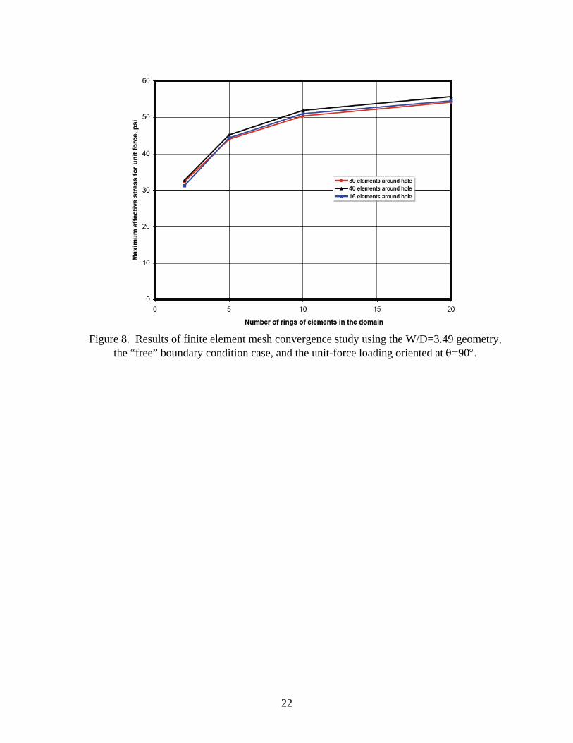
Results are generated for the “free” boundary condition case (see Figure 6b) with the unit-force line of action oriented at θ=90°. The maximum effective stress as a function of the spatial discretization is shown in Figure 8 to depend more on the number of element rings between the edge of the hole and the edge of the domain (across a plane-stress ligament) than on the number of element spokes around the hole. For a given number of element rings across a plane-stress ligament, the maximum effective stress is essentially independent of the number of element spokes around the hole. This result for a single direction of the unit force is not a general conclusion for pin-loaded holes since only a linear elastic response is considered. As the unit-force line of action changes (i.e., changes in the angle θ), the pin-bearing condition also changes for at least two reasons. One reason for the change is because of the geometry approximation of the hole boundary (i.e., series of straight line segments when 4-node elements are used), and another reason is because of the limited number of discrete nodal contact points. Both reasons are influenced by the finite element spatial discretization around the hole. Surface-to-surface contact modeling with an analytical contact-surface definition (i.e., the surface node locations are used to define a smooth analytical surface for contact) does address the discrete nodal contact modeling issue but does not address the curved-boundary approximation issue. Thus, the finite element spatial discretization shown in Figure 5 (and on the right side of Figure 7d) , which represents the most refined finite element mesh considered, is used in all subsequent studies reported herein.

7

Effect of Pin-Bearing Modeling Next, the effect of pin-bearing modeling is studied. In the present paper, two two-dimensional joint modeling approaches are considered. The pin itself is not modeled explicitly in these two-dimensional analyses, but rather it is simulated as a near-rigid (very stiff) member that generates a bearing load along the hole boundary. The pin-bearing response is simulated using either linear spring elements or nonlinear spring (gap) elements. Linear spring elements assume the same behavior regardless of whether the spring is compressed or extended. Tensile forces are generated on the edge of the hole opposite where compressive bearing forces are generated, and true pin-bearing behavior is not simulated. Nonlinear spring or gap elements assume that no tensile forces can be generated when the spring is extended and a gap results, while compressive bearing forces are generated when the spring is compressed to simulate the true pin-bearing behavior.

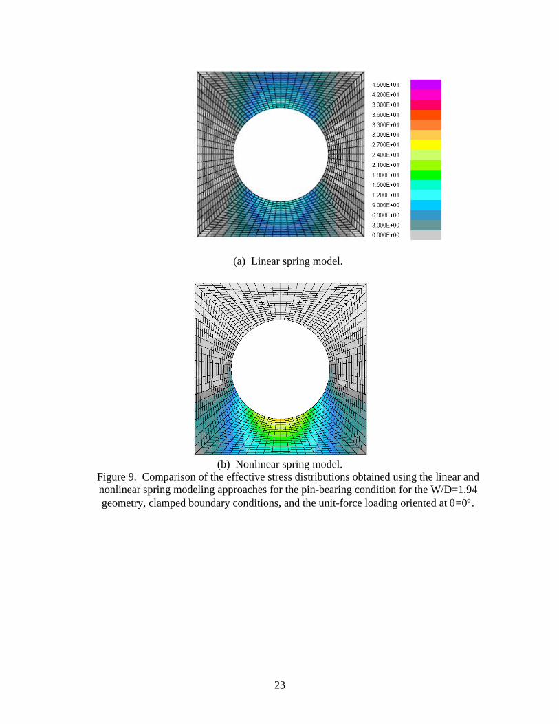
A comparison of the effective stress distributions obtained for the linear and nonlinear spring modeling approaches to simulate the pin-bearing behavior for a two-dimensional joint is presented in Figure 9 using the same range for the effective stress in both cases (0 to 45 psi). For this comparison, the W/D=1.94 domain geometry is used with the “clamped” boundary condition case of Figure 6b, and the unit-force line of action is oriented at θ=0°. The effective stress distribution obtained for the linear spring model is shown in Figure 9a and illustrates that the entire surface around the hole is loaded. In some regions, the pin is “pulling” on the edge of the hole; while in other regions, the pin is “pushing” or bearing against the edge of the hole. This type of response is inconsistent with the physical behavior of pin-loaded holes. The effective stress distribution based on the nonlinear spring model is shown in Figure 9b and illustrates a physically consistent pin-bearing surface response. The bearing behavior is simulated through the use of nonlinear spring elements that generate zero force when extended (i.e., generates a gap) and a bearing force when shortened or compressed. Hence, the nonlinear spring model is used in the remainder of the studies reported in the present paper, except where noted.

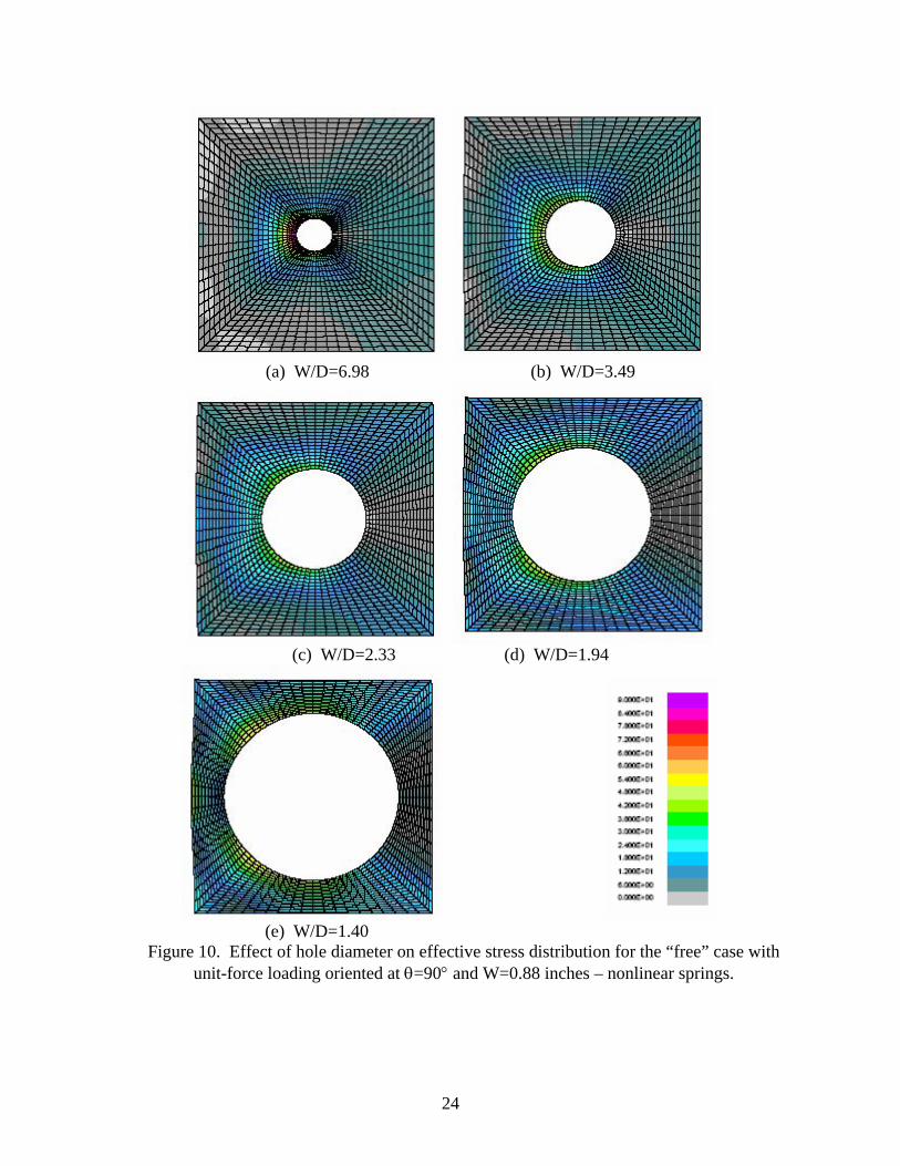
Effect of Hole Diameter The effect of hole diameter on the effective stress distribution is studied further for the case of the “free” boundary conditions with the unit-force line of action as 90°. Five different values of the W/D ratio are analyzed where the value of W is held constant (W=0.88 inches). The values of the W/D ratio considered are listed in Table 2 and are selected based on ratios of D/D0. These finite element models assume that the pin size also changes as the hole diameter changes. Furthermore, the pin surface and the hole boundary are assumed to be in direct contact – stress free, no pre-load, and no clearances.

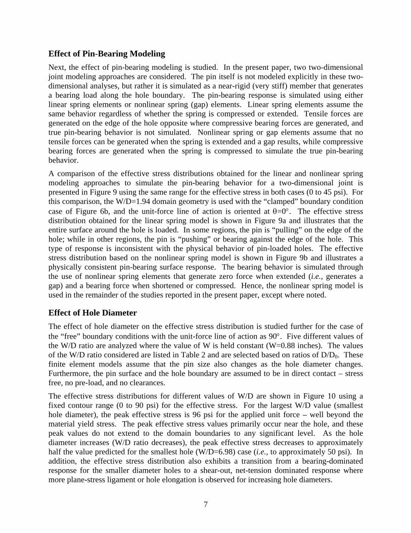
The effective stress distributions for different values of W/D are shown in Figure 10 using a fixed contour range (0 to 90 psi) for the effective stress. For the largest W/D value (smallest hole diameter), the peak effective stress is 96 psi for the applied unit force – well beyond the material yield stress. The peak effective stress values primarily occur near the hole, and these peak values do not extend to the domain boundaries to any significant level. As the hole diameter increases (W/D ratio decreases), the peak effective stress decreases to approximately half the value predicted for the smallest hole (W/D=6.98) case (i.e., to approximately 50 psi). In addition, the effective stress distribution also exhibits a transition from a bearing-dominated response for the smaller diameter holes to a shear-out, net-tension dominated response where more plane-stress ligament or hole elongation is observed for increasing hole diameters.

8

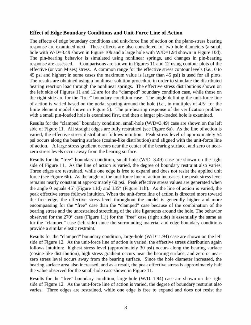
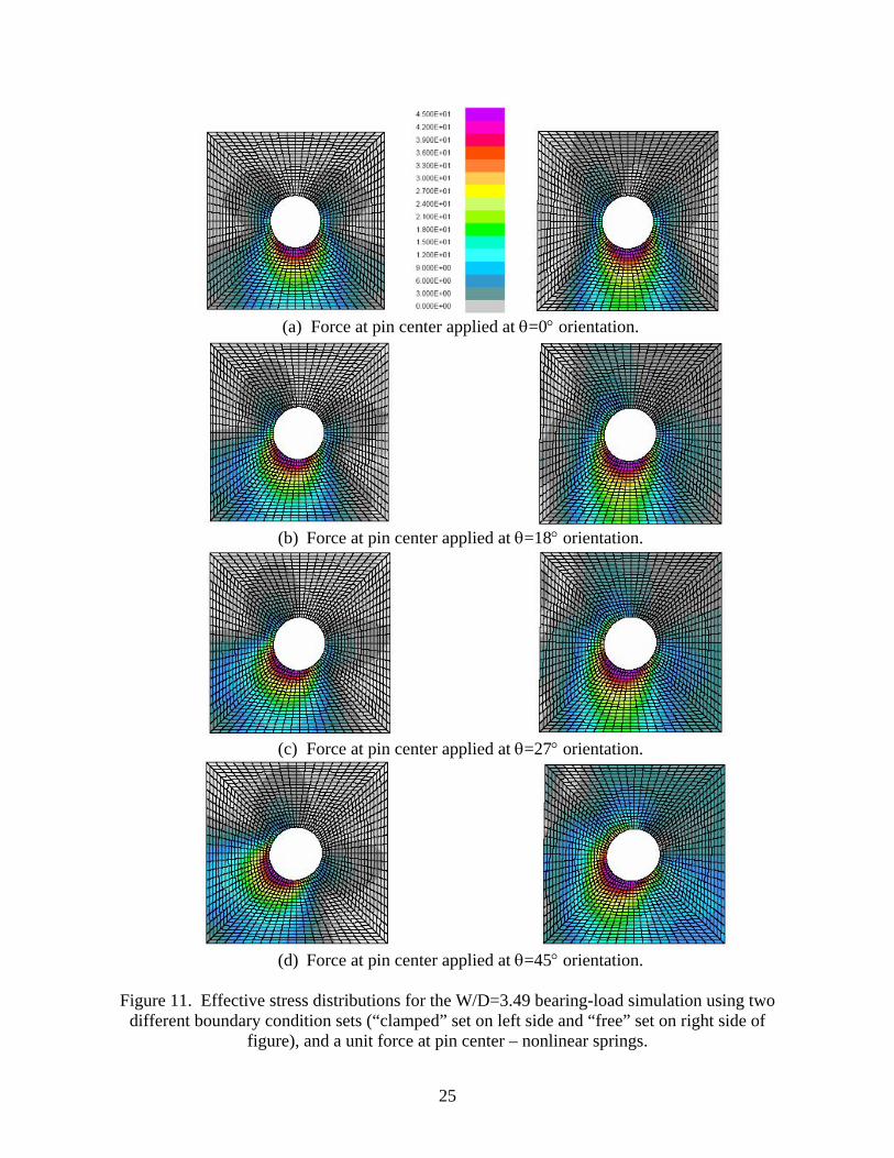
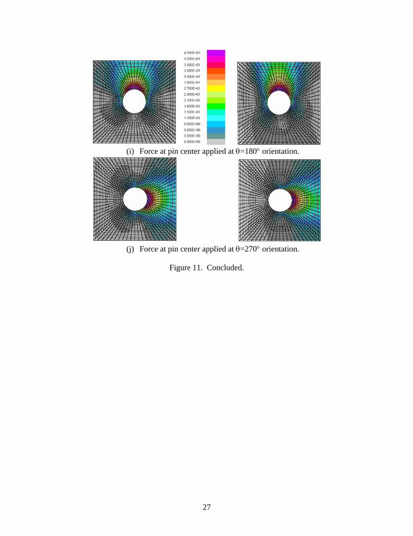
Effect of Edge Boundary Conditions and Unit-Force Line of Action The effects of edge boundary conditions and unit-force line of action on the plane-stress bearing response are examined next. These effects are also considered for two hole diameters (a small hole with W/D=3.49 shown in Figure 10b and a large hole with W/D=1.94 shown in Figure 10d). The pin-bearing behavior is simulated using nonlinear springs, and changes in pin-bearing response are assessed. Comparisons are shown in Figures 11 and 12 using contour plots of the effective (or von Mises) stress. A common range for the effective stress contour levels (i.e., 0 to 45 psi and higher; in some cases the maximum value is larger than 45 psi) is used for all plots. The results are obtained using a nonlinear solution procedure in order to simulate the distributed bearing reaction load through the nonlinear springs. The effective stress distributions shown on the left side of Figures 11 and 12 are for the “clamped” boundary condition case, while those on the right side are for the “free” boundary condition case. The angle defining the unit-force line of action is varied based on the nodal spacing around the hole (i.e., in multiples of 4.5° for the finite element model shown in Figure 5). The pin-bearing response of the verification problem with a small pin-loaded hole is examined first, and then a larger pin-loaded hole is examined.

Results for the “clamped” boundary condition, small-hole (W/D=3.49) case are shown on the left side of Figure 11. All straight edges are fully restrained (see Figure 6a). As the line of action is varied, the effective stress distribution follows intuition. Peak stress level of approximately 54 psi occurs along the bearing surface (cosine-like distribution) and aligned with the unit-force line of action. A large stress gradient occurs near the center of the bearing surface, and zero or near-zero stress levels occur away from the bearing surface.

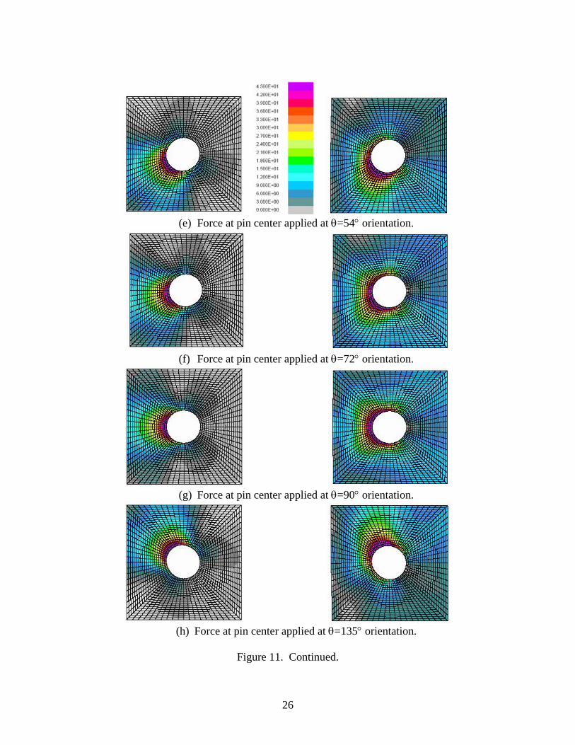
Results for the “free” boundary condition, small-hole (W/D=3.49) case are shown on the right side of Figure 11. As the line of action is varied, the degree of boundary restraint also varies. Three edges are restrained, while one edge is free to expand and does not resist the applied unit force (see Figure 6b). As the angle of the unit-force line of action increases, the peak stress level remains nearly constant at approximately 60 psi. Peak effective stress values are generated when the angle θ equals 45° (Figure 11d) and 135° (Figure 11h). As the line of action is varied, the peak effective stress follows intuition. When the unit-force line of action is directed more toward the free edge, the effective stress level throughout the model is generally higher and more encompassing for the “free” case than the “clamped” case because of the combination of the bearing stress and the unrestrained stretching of the side ligaments around the hole. The behavior observed for the 270° case (Figure 11j) for the “free” case (right side) is essentially the same as for the “clamped” case (left side) since the surrounding material and edge boundary conditions provide a similar elastic restraint.

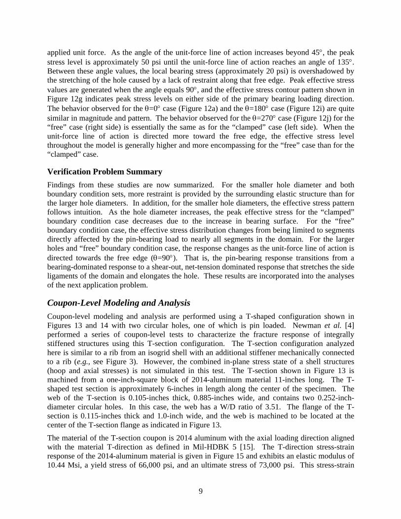
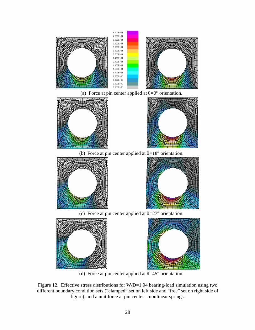
Results for the “clamped” boundary condition, large-hole (W/D=1.94) case are shown on the left side of Figure 12. As the unit-force line of action is varied, the effective stress distribution again follows intuition: highest stress level (approximately 30 psi) occurs along the bearing surface (cosine-like distribution), high stress gradient occurs near the bearing surface, and zero or near-zero stress level occurs away from the bearing surface. Since the hole diameter increased, the bearing surface area also increased, and as a result, the peak effective stress is approximately half the value observed for the small-hole case shown in Figure 11.

Results for the “free” boundary condition, large-hole (W/D=1.94) case are shown on the right side of Figure 12. As the unit-force line of action is varied, the degree of boundary restraint also varies. Three edges are restrained, while one edge is free to expand and does not resist the

9

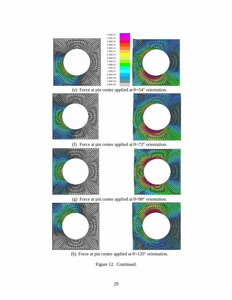
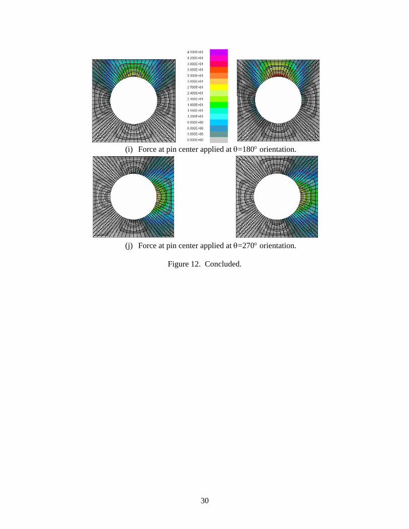
applied unit force. As the angle of the unit-force line of action increases beyond 45°, the peak stress level is approximately 50 psi until the unit-force line of action reaches an angle of 135°. Between these angle values, the local bearing stress (approximately 20 psi) is overshadowed by the stretching of the hole caused by a lack of restraint along that free edge. Peak effective stress values are generated when the angle equals 90°, and the effective stress contour pattern shown in Figure 12g indicates peak stress levels on either side of the primary bearing loading direction. The behavior observed for the θ=0° case (Figure 12a) and the θ=180° case (Figure 12i) are quite similar in magnitude and pattern. The behavior observed for the θ=270° case (Figure 12j) for the “free” case (right side) is essentially the same as for the “clamped” case (left side). When the unit-force line of action is directed more toward the free edge, the effective stress level throughout the model is generally higher and more encompassing for the “free” case than for the “clamped” case.

Verification Problem Summary Findings from these studies are now summarized. For the smaller hole diameter and both boundary condition sets, more restraint is provided by the surrounding elastic structure than for the larger hole diameters. In addition, for the smaller hole diameters, the effective stress pattern follows intuition. As the hole diameter increases, the peak effective stress for the “clamped” boundary condition case decreases due to the increase in bearing surface. For the “free” boundary condition case, the effective stress distribution changes from being limited to segments directly affected by the pin-bearing load to nearly all segments in the domain. For the larger holes and “free” boundary condition case, the response changes as the unit-force line of action is directed towards the free edge (θ=90°). That is, the pin-bearing response transitions from a bearing-dominated response to a shear-out, net-tension dominated response that stretches the side ligaments of the domain and elongates the hole. These results are incorporated into the analyses of the next application problem.

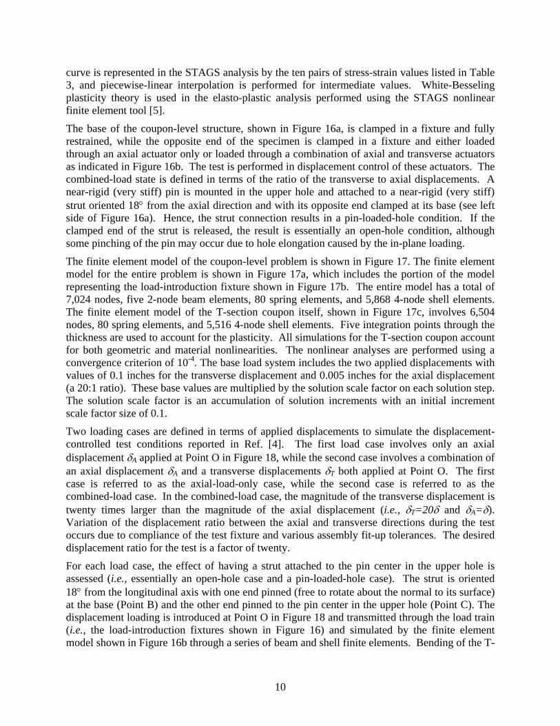
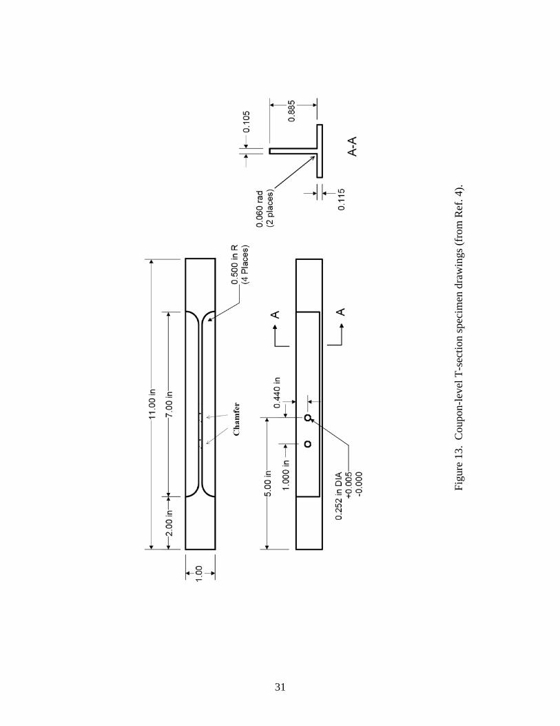
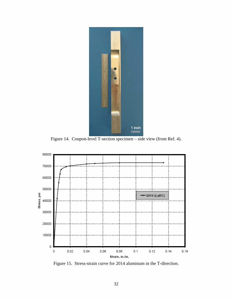
Coupon-Level Modeling and Analysis Coupon-level modeling and analysis are performed using a T-shaped configuration shown in Figures 13 and 14 with two circular holes, one of which is pin loaded. Newman et al. [4] performed a series of coupon-level tests to characterize the fracture response of integrally stiffened structures using this T-section configuration. The T-section configuration analyzed here is similar to a rib from an isogrid shell with an additional stiffener mechanically connected to a rib (e.g., see Figure 3). However, the combined in-plane stress state of a shell structures (hoop and axial stresses) is not simulated in this test. The T-section shown in Figure 13 is machined from a one-inch-square block of 2014-aluminum material 11-inches long. The T-shaped test section is approximately 6-inches in length along the center of the specimen. The web of the T-section is 0.105-inches thick, 0.885-inches wide, and contains two 0.252-inch-diameter circular holes. In this case, the web has a W/D ratio of 3.51. The flange of the T-section is 0.115-inches thick and 1.0-inch wide, and the web is machined to be located at the center of the T-section flange as indicated in Figure 13.

The material of the T-section coupon is 2014 aluminum with the axial loading direction aligned with the material T-direction as defined in Mil-HDBK 5 [15]. The T-direction stress-strain response of the 2014-aluminum material is given in Figure 15 and exhibits an elastic modulus of 10.44 Msi, a yield stress of 66,000 psi, and an ultimate stress of 73,000 psi. This stress-strain

10

curve is represented in the STAGS analysis by the ten pairs of stress-strain values listed in Table 3, and piecewise-linear interpolation is performed for intermediate values. White-Besseling plasticity theory is used in the elasto-plastic analysis performed using the STAGS nonlinear finite element tool [5].

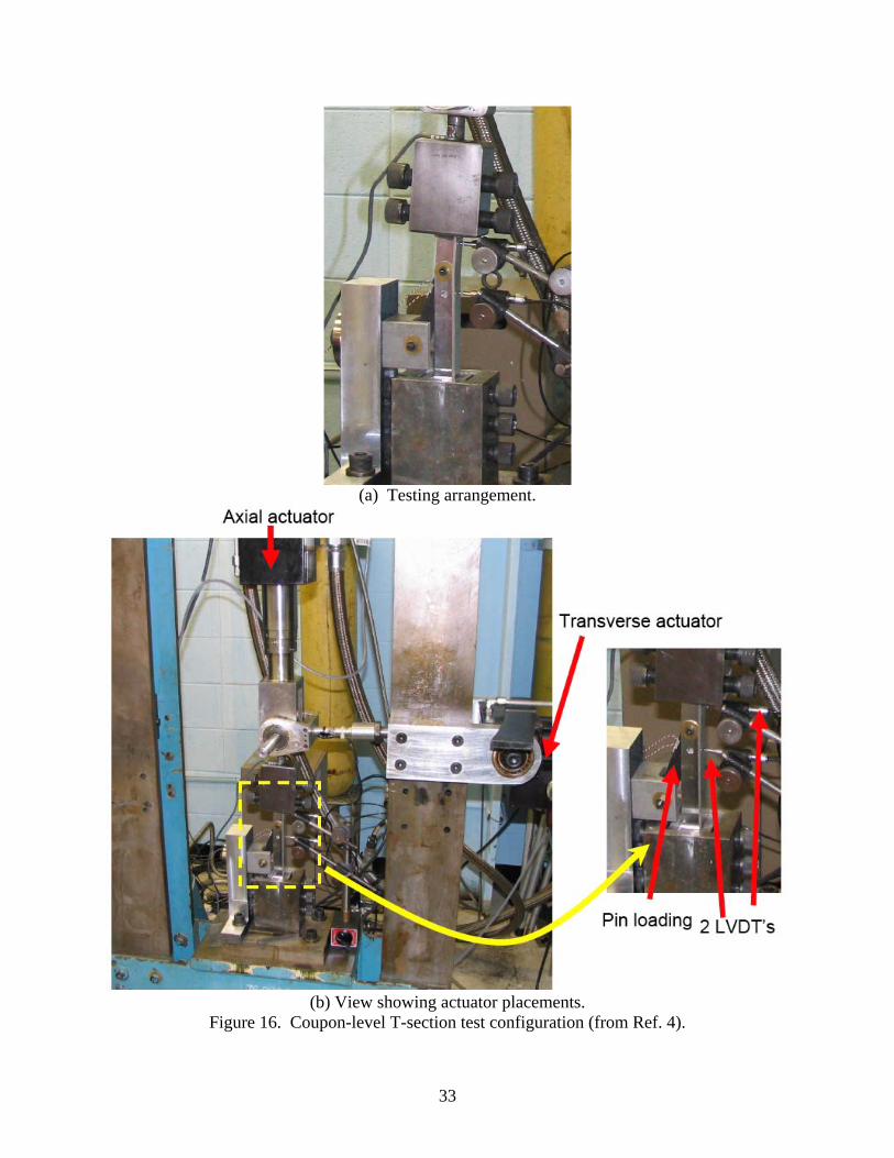
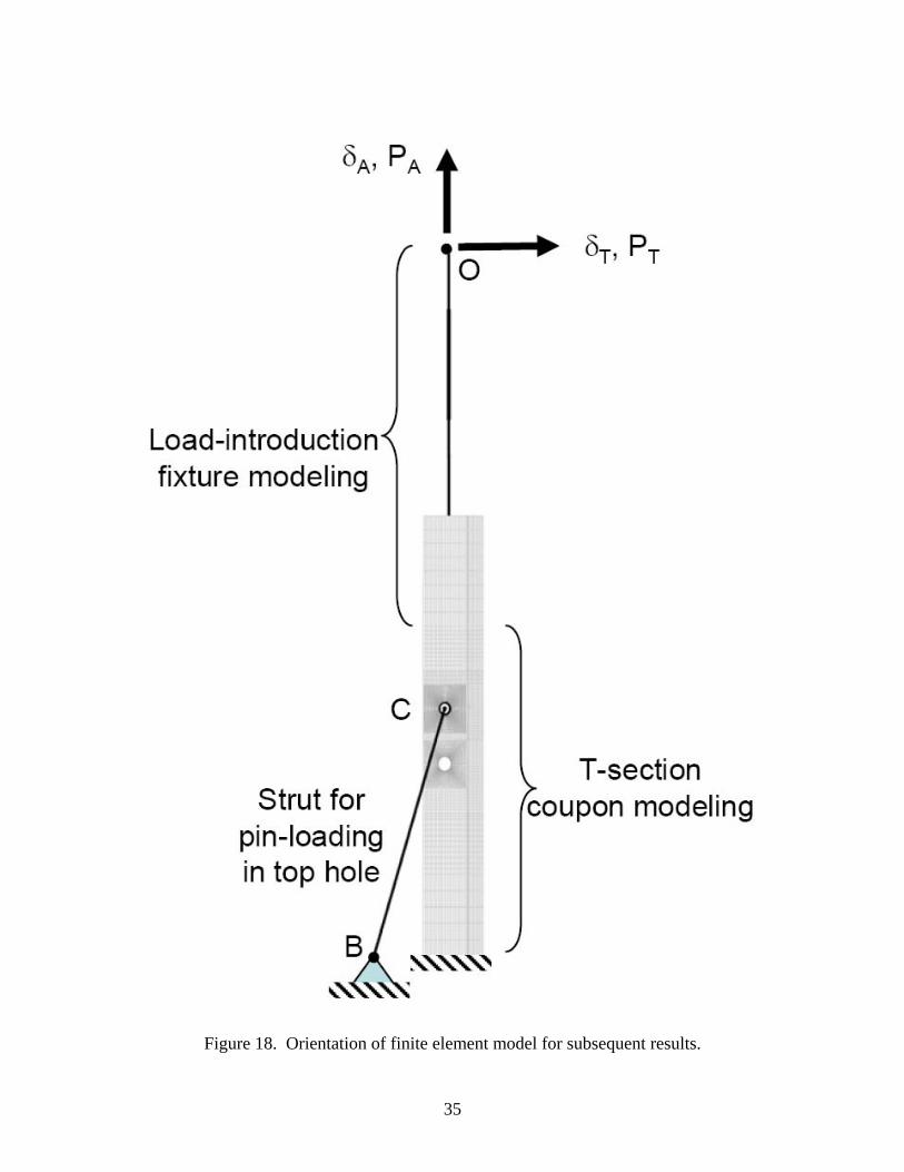
The base of the coupon-level structure, shown in Figure 16a, is clamped in a fixture and fully restrained, while the opposite end of the specimen is clamped in a fixture and either loaded through an axial actuator only or loaded through a combination of axial and transverse actuators as indicated in Figure 16b. The test is performed in displacement control of these actuators. The combined-load state is defined in terms of the ratio of the transverse to axial displacements. A near-rigid (very stiff) pin is mounted in the upper hole and attached to a near-rigid (very stiff) strut oriented 18° from the axial direction and with its opposite end clamped at its base (see left side of Figure 16a). Hence, the strut connection results in a pin-loaded-hole condition. If the clamped end of the strut is released, the result is essentially an open-hole condition, although some pinching of the pin may occur due to hole elongation caused by the in-plane loading.

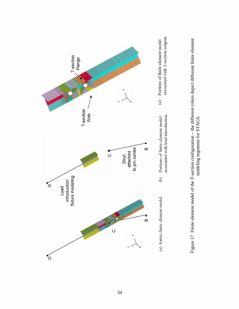
The finite element model of the coupon-level problem is shown in Figure 17. The finite element model for the entire problem is shown in Figure 17a, which includes the portion of the model representing the load-introduction fixture shown in Figure 17b. The entire model has a total of 7,024 nodes, five 2-node beam elements, 80 spring elements, and 5,868 4-node shell elements. The finite element model of the T-section coupon itself, shown in Figure 17c, involves 6,504 nodes, 80 spring elements, and 5,516 4-node shell elements. Five integration points through the thickness are used to account for the plasticity. All simulations for the T-section coupon account for both geometric and material nonlinearities. The nonlinear analyses are performed using a convergence criterion of 10-4. The base load system includes the two applied displacements with values of 0.1 inches for the transverse displacement and 0.005 inches for the axial displacement (a 20:1 ratio). These base values are multiplied by the solution scale factor on each solution step. The solution scale factor is an accumulation of solution increments with an initial increment scale factor size of 0.1.

Two loading cases are defined in terms of applied displacements to simulate the displacement-controlled test conditions reported in Ref. [4]. The first load case involves only an axial displacement δA applied at Point O in Figure 18, while the second case involves a combination of an axial displacement δA and a transverse displacements δT both applied at Point O. The first case is referred to as the axial-load-only case, while the second case is referred to as the combined-load case. In the combined-load case, the magnitude of the transverse displacement is twenty times larger than the magnitude of the axial displacement (i.e., δT=20δ and δA=δ). Variation of the displacement ratio between the axial and transverse directions during the test occurs due to compliance of the test fixture and various assembly fit-up tolerances. The desired displacement ratio for the test is a factor of twenty.

For each load case, the effect of having a strut attached to the pin center in the upper hole is assessed (i.e., essentially an open-hole case and a pin-loaded-hole case). The strut is oriented 18° from the longitudinal axis with one end pinned (free to rotate about the normal to its surface) at the base (Point B) and the other end pinned to the pin center in the upper hole (Point C). The displacement loading is introduced at Point O in Figure 18 and transmitted through the load train (i.e., the load-introduction fixtures shown in Figure 16) and simulated by the finite element model shown in Figure 16b through a series of beam and shell finite elements. Bending of the T-

11

section coupon occurs even for the axial-load-only case due to the assembly eccentricities and the load-introduction process.

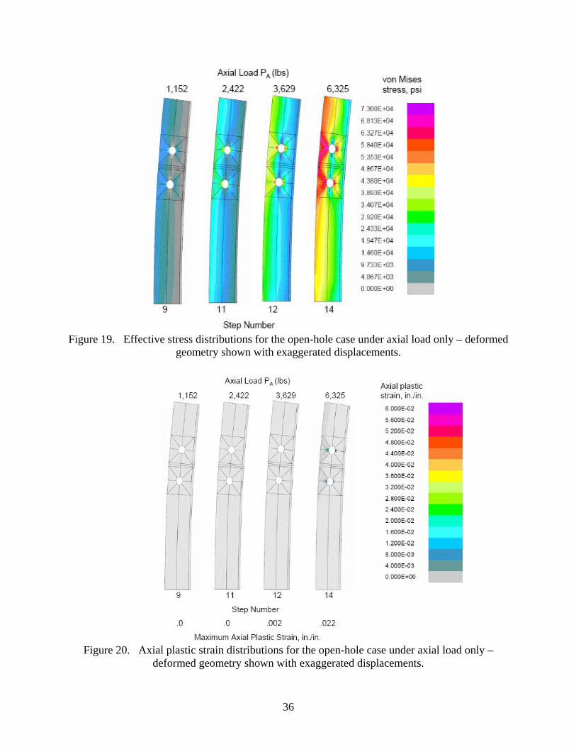
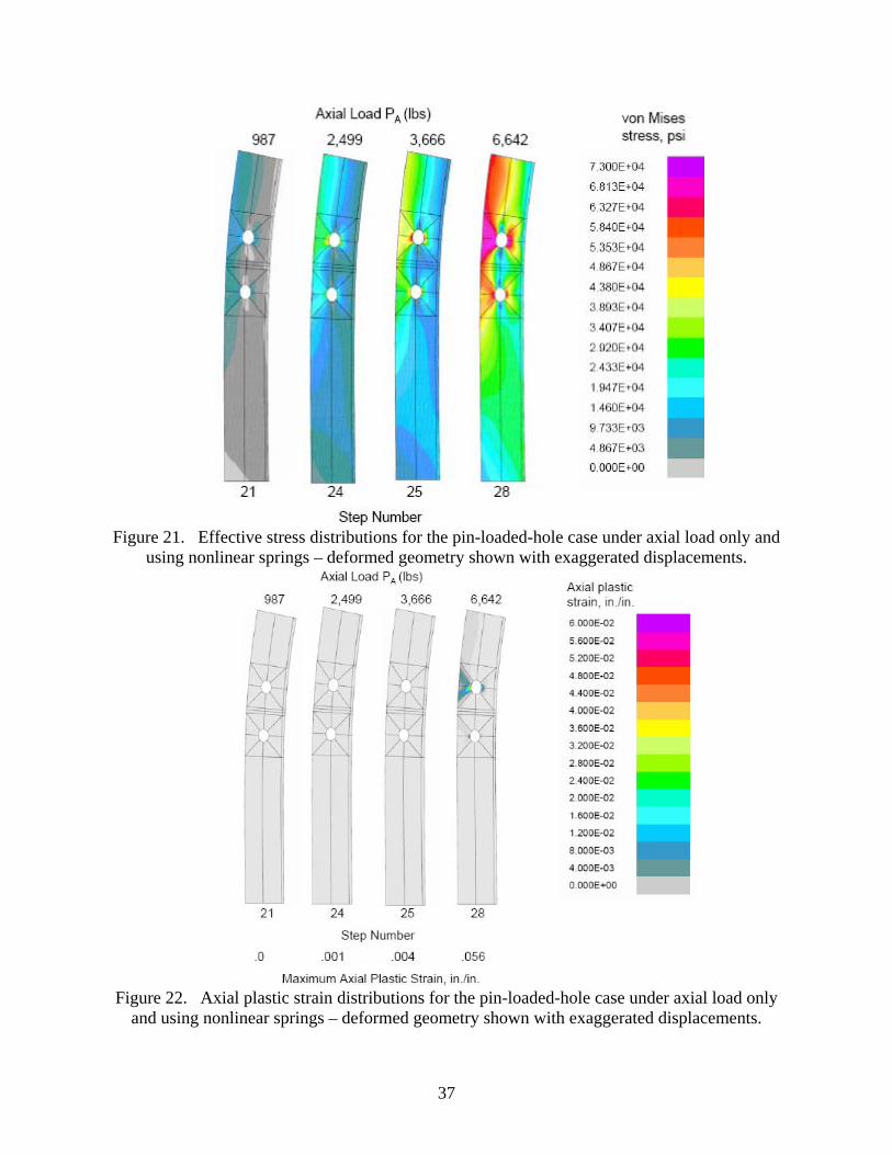
Axial-Load-Only Case For the axial-load-only case, results are obtained for the open-hole case (see Figures 19 and 20) and for the pin-loaded-hole case (see Figures 21 and 22). Effective stress distributions displayed on the deformed geometry with exaggerated displacements are shown in Figure 19 for the open-hole case and in Figure 21 for the pin-loaded-hole case. Contour plots of the effective stress distributions at different levels of the axial load are presented with the range of the effective stress set from zero to 73,000 psi (ultimate stress value) where the yield stress is 66,000 psi. The nonlinear solution step number and axial load PA for each distribution are indicated on the figures. Axial plastic strain distributions displayed on the deformed geometry with exaggerated displacements are shown in Figure 20 for the open-hole case and in Figure 22 for the pin-loaded-hole case. Contour plots of the axial strain distributions at different levels of the axial load are presented with the range of the axial plastic strain set from zero to 0.06 in./in. where the elastic limit is approximately ±0.006 in./in. Even though only an axial displacement is applied, stretching and bending of the T-section coupon occurs due to eccentricities in the system. Nonlinear solutions were computed up to a maximum applied axial displacement δA of 0.03 inches (i.e., δT=20δA =0.6 inches).

Results for the open-hole case are shown in Figures 19 and 20 for four nonlinear solution steps (i.e., Steps 9, 11, 12, and 14). The open-hole case exhibits higher effective stresses in the “free” regions of the T-section web as shown in Figure 18 since that region has less axial stiffness (i.e., less elastic support from surrounding material). As the axial load increases, stress concentrations near both holes are evident. Axial plastic strain distributions are shown in Figure 20 for the open-hole case. Steps 9, 11 and 12 in Figure 20 indicate no or minimal plastic strains present. As the applied displacement continues to increase, tensile axial plastic strains also increase near the hole boundary as indicated in Figure 20. At the final load step (i.e., Step 14), axial plastic strain develops near both holes and extends along the full length of the outer “free” region of the T-section web. However, these strain levels are well below the ultimate strain value.

Results for the pin-loaded-hole case are shown in Figures 21 and 22 for four nonlinear solution steps (i.e., Steps 21, 24, 25, and 28). Due to the presence of the nonlinear springs to simulate the pin-bearing response at the upper hole, the nonlinear solution required more solution steps compared to the open-hole case (i.e., 28 steps compared to 14 steps). In this case, the upper hole develops stress concentrations much earlier than they do for the lower hole (see Figure 21). Tensile axial plastic strains are evident in Figure 22 emanating from near the upper hole first and extend to the outer “free” region of the T-section web.

In both cases, the local stress field is dominated by the stretching behavior along the free edge of the T-section web. The stretching causes a stress concentration to develop near the holes. For the open-hole case, stress concentrations develop at both holes simultaneously and in concert with each other. When the strut is “attached”, pin-bearing loads result at the upper hole and tend to shield the lower hole to some extent. However, these local bearing compressive stresses at the upper hole are overshadowed by the tensile in-plane stresses in the outer “free” portions of the T-section web. Hence, for the axial-load-only case, the T-section exhibits plastic deformations; however, they are well within the material ultimate capability. Next, the combined-load case is assessed.

12

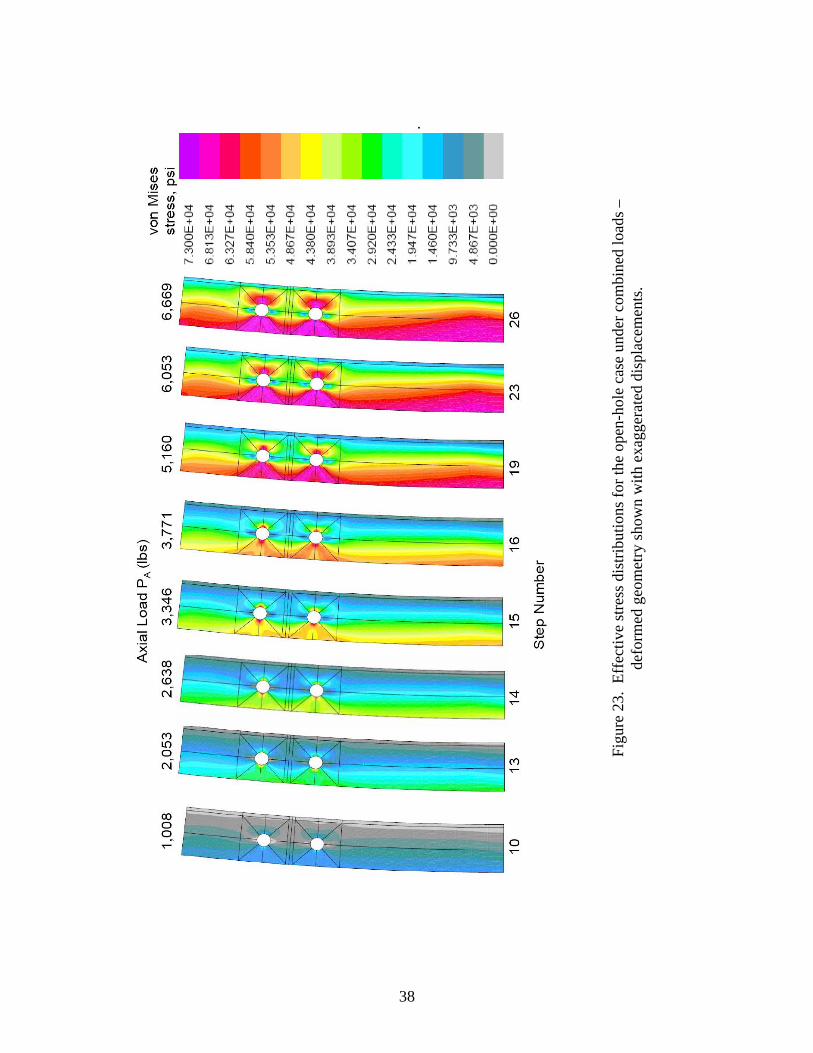
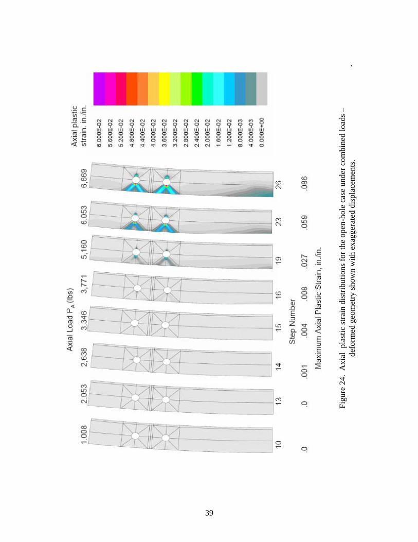
Combined-Load Case For the combined-load case, results are again obtained for the open-hole case (see Figures 23 and 24) and for the pin-loaded-hole case (see Figures 24 and 25). Similar sets of effective stress contour are presented in Figures 23 and 25. Again, contour plots of the effective stress distributions at different levels of the axial load are presented with the range of the effective stress set from zero to 73,000 psi (ultimate stress value) where the yield stress is 66,000 psi. The nonlinear solution step number and axial load PA for each distribution are indicated on the figures. Axial plastic strain distributions are shown in Figures 24 and 26. Contour plots of the axial strain distributions at different levels of axial loading are presented with the range of the axial plastic strain set from zero to 0.06 in./in. where the elastic limit is approximately ±0.006 in./in. Again, the open-hole case required only about half the number of nonlinear solution steps that the pin-loaded-hole case required (i.e., 26 steps compared to 56 steps).

The effective stress distributions for the open-hole, combined-load case are presented in Figure 23 for eight nonlinear solution steps (i.e., Steps 10, 13, 14, 15, 16, 19, 21, and 26). These distributions indicate that as the axial load increased, the free edge of the T-section web is stressed more than the edge closest to the T-section flange along the entire specimen length. Stress concentrations near both the upper and lower holes quickly develop and both holes exhibit elongation. Axial plastic strain distributions are shown in Figure 24 for the same solution steps. Plastic deformations are also evident opposite the free edge of the T-section web near the holes. Plastic strains spread along the free edge of the T-section web with high localized plastic strains near the edges of both holes. The maximum axial load from the analysis is 6,669 pounds when the applied displacements reached their maximum values (i.e., δT=20δA =0.6 inches).

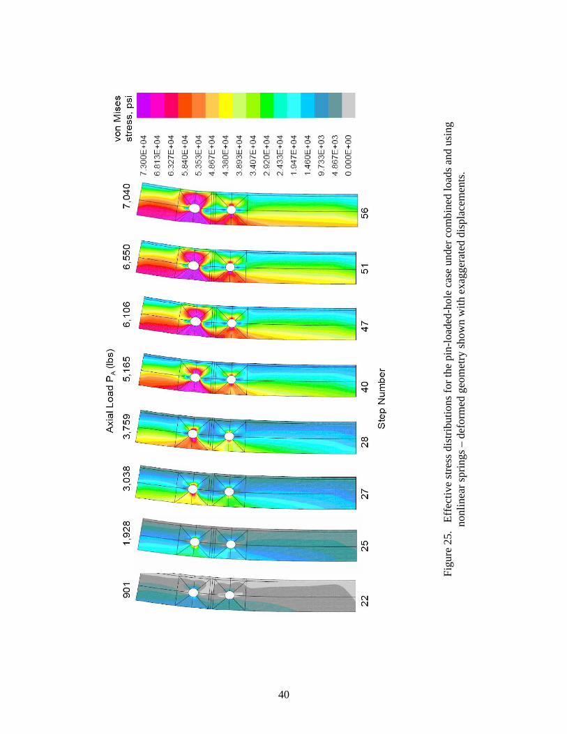
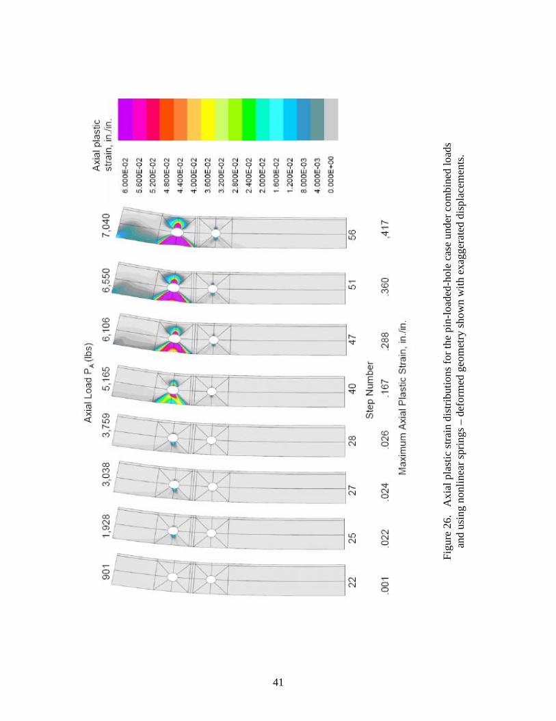
The effective stress distributions for the pin-loaded-hole, combined-load case are presented in Figure 25 for eight nonlinear solution steps (i.e., Steps 22, 25, 27, 28, 40, 47, 51, and 56). These distributions indicate that as the axial load is increased, the portion of the T-section web near the free edge of the upper hole is stressed more than any other region. While there is evidence of local compressive bearing due to the pin-load reaction, the tensile in-plane response due to the applied displacements dominates the response. Axial plastic strain distributions are shown in Figure 26 for the same solution steps. Plastic deformations develop opposite the edge of the pin-loaded hole nearest the free edge of the T-section web – similar to the open-hole case. However, these plastic deformations develop sooner, and the tensile axial plastic strains are much larger near the upper hole than in the open-hole case (compare distributions shown in Figure 24 with those shown in Figure 26). The maximum axial load from the analysis is 7,040 pounds when the applied displacements reached their maximum values (i.e., δT=20δA =0.6 inches) – within 6% of the open-hole case. These results indicate that the pin-loaded-hole, combined-load case is the most severe case considered. The analysis predicted axial plastic strains that exceed the material ultimate strain limit near the upper hole prior to reaching the maximum axial load.

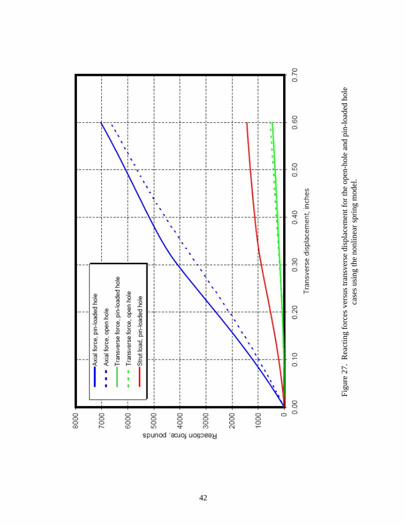
In addition, for the combined-load case, the reacted axial, transverse, and strut forces as functions of the applied transverse displacement are shown in Figure 27. The solid curves represent the pin-loaded-hole case, and the dashed curves represent the open-hole case (no strut loads are generated). The response of the pin-loaded-hole case is somewhat stiffer than the open-hole case. Approximately 20% of the axial reaction force is transferred to the strut that is attached to the center of the pin in the upper hole. As expected, the pin-loaded-hole case exhibits a smaller transverse displacement for the same axial reaction force compared to the results for the open-hole case. Ref. [4] reports test results for two 20:1 displacement ratio tests. The

13

average maximum axial load is 5,135 pounds, and the average maximum transverse displacement is 0.595 inches. However, the observed compliance in the load introduction fixture accounts for approximately 0.09 inches of the transverse displacement. Comparison of this average test data from Table 7 of Ref. [4] (5,135 pounds at 0.505 inches) with the nonlinear analysis results for the combined-load, pin-loaded-hole case (5,160 pounds at 0.398 inches) indicates a consistency in the results. Other uncertainties in the test may need to be reflected in the analysis.

Effect of Pin-Bearing Modeling As a final analysis, the pin-loaded-hole, combined-load case is analyzed using the linear spring model (see Table 1) to simulate the pin-bearing behavior. While previous studies in the present paper indicate that such a modeling approach generates non-physical behavior, the linear spring modeling approach is frequently used in practice. The analyses performed for this section include elastic-plastic material behavior and large deformations for the T-section coupon. Effective stress and axial plastic strain results are compared to corresponding results obtained using a nonlinear spring model for the pin-bearing response. In the linear spring model, the boundary of the hole is “pulled” and “pushed” as the springs around the upper hole deform. In the nonlinear spring model, the boundary of the hole is only “pushed” when the springs are compressed usually a 180° sector.

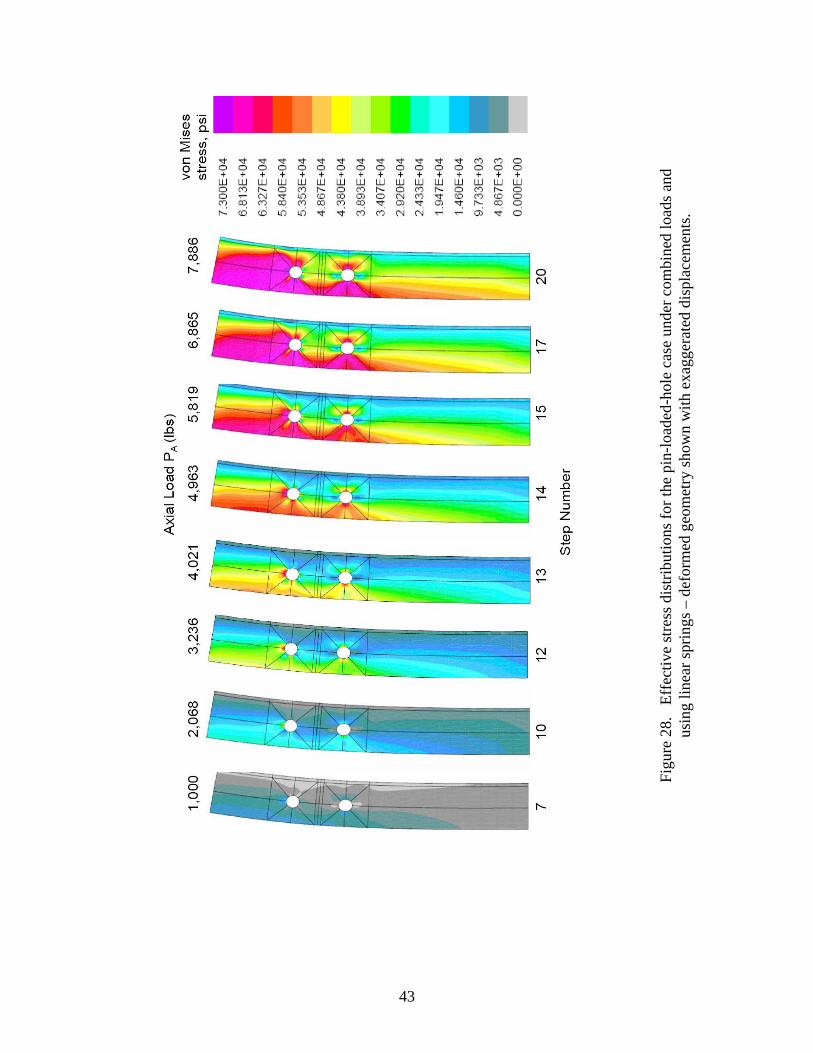
The effective stress distributions are presented in Figure 28. Again, these contour plots of the effective stress distributions are for different nonlinear solution steps (i.e., Steps 7, 10, 12, 13, 14, 15, 17, and 20), and the axial load level for each step is indicated on the figure. As in previous cases, the range of the effective stress contour levels is set from zero to 73,000 psi (ultimate stress value). In this linear spring analysis model, the pin both pushes (compressive bearing force) and pulls (tensile force) on opposite edges of the hole boundary as the applied displacements increase. These imposed displacements result in high in-plane stresses along the free edge of the specimen due to the elastic restraint of the surrounding material. Pin bearing generates a local compressive in-plane stress, which when superimposed on the primary stress field, results in a stress level along the bearing surface of the pin that is lower than the stress level at θ=90°. For the linear spring model, a local tensile in-plane stress is generated near the hole surface opposite the compressive bearing region that combines with the primary stress field resulting in a higher tensile in-plane stress level. This response is not present in the actual structure.

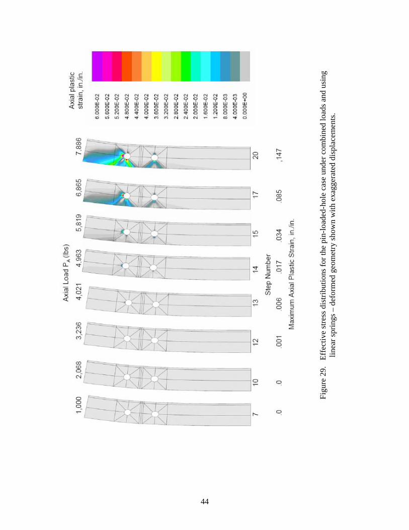
Axial plastic strain distributions for the same solution steps are shown in Figure 29. Contour plots of the axial strain distributions at different levels of applied loading are presented with the range of the axial plastic strain set from zero to 0.06 in./in. As the axial load increases, plastic deformations develop near both holes. Higher tensile axial plastic strains emanate around the top hole region and dominate the response. Plastic strains are evident in Figure 29 in the upper region of the top hole – a non-bearing surface because of the linear spring modeling approach. The maximum sustained axial load from the analysis is 7,886 pounds – 18% higher than the open-hole, combined-load case.

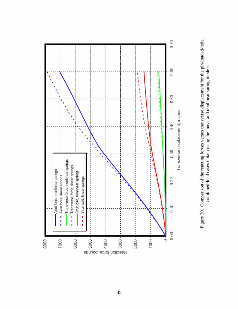
A comparison of the reacted axial, transverse, and strut forces obtained from the linear and nonlinear spring models as functions of the applied transverse displacement is shown in Figure 30 for the pin-loaded-hole case. The solid curves represent the results obtained using the nonlinear spring model, and the dashed curves represent the results obtained using the linear

14

spring model. The response of the linear spring model is somewhat stiffer than the nonlinear spring model, although the trends are nearly identical. However, the peak reacting forces for the nonlinear spring model are approximately half the values predicted by the linear spring model due in part to the “pushing” and “pulling” nature of the linear springs.

Concluding Remarks Bearing-load response for a pin-loaded hole is studied. First, modeling and analysis aspects of a pin-loaded hole are considered. Second, the use of nonlinear springs to simulate the pin-bearing contact condition is demonstrated including the identification of modeling issues associated with using linear springs. Next, the effect of hole diameter on the local response is determined. As hole diameter increases, the response changes from a bearing-dominated response for plates with small holes (large values of W/D) to an in-plane shear-out-dominated ligament response for plates with larger holes (small values of W/D).

Results from the parametric studies indicate several lessons learned. First, in a two-dimensional finite element analysis model of a mechanical connection, the use of nonlinear spring (or gap) elements to simulate bearing in pin-loaded holes is a good computational alternative to three-dimensional contact simulations. Second, the spatial discretization within the two-dimensional model needs to be sufficient to reflect the bearing behavior and is more sensitive to the number of “spokes” of elements than the number of “rings” of elements. Third, as the size of the hole relative to the width of the strip containing the hole increases, a transition in the structural response of the connection is observed.

Application to a more complex structure is also illustrated. The T-section coupon configuration is representative of a separate stiffener mechanically connected to a rib of an isogrid panel. For the coupon configuration, the pin-loaded-hole case resulted in higher local stresses around the hole. For a series of bolts, the consequence of the last bolt carrying most of the load is that local failures will most likely occur at that location. Redistribution of load to other bolts may occur provided the plastic deformation at the first bolt does not result in local material failures that extend to, and possibly through, the T-section flange thickness. In any case, simulating the bearing contact response of pin-loaded holes needs to be included in the finite element analysis model, and the use of nonlinear springs is an attractive and accurate alternative to explicit contact modeling.

15

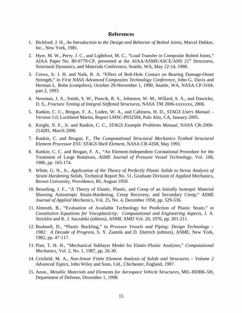
References 1. Bickford. J. H., An Introduction to the Design and Behavior of Bolted Joints, Marcel Dekker,

Inc., New York, 1981.

2. Hyer, M. W., Perry, J. C., and Lightfoot, M. C., “Load Transfer in Composite Bolted Joints,” AIAA Paper No. 80-0779-CP, presented at the AIAA/ASME/ASCE/AHS 21st Structures, Structural Dynamics, and Materials Conference, Seattle, WA, May 12-14, 1980.

3. Crews, Jr. J. H. and Naik, R. A. “Effect of Bolt-Hole Contact on Bearing Damage-Onset Strength,” in First NASA Advanced Composites Technology Conference, John G. Davis and Herman L. Bohn (compilers), October 29-November 1, 1990, Seattle, WA, NASA CP-3104, part 2, 1993.

4. Newman, J. A., Smith, S. W., Piascik, R. S., Johnston, W. M., Willard, S. A., and Dawicke, D. S., Fracture Testing of Integral Stiffened Structures, NASA TM 2006-xxxxxxx, 2006.

5. Rankin, C. C., Brogan, F. A., Loden, W. A., and Cabiness, H. D., STAGS Users Manual – Version 5.0, Lockheed Martin, Report LMSC-P032594, Palo Alto, CA, January 2005.

6. Knight, N. F., Jr. and Rankin, C. C., STAGS Example Problems Manual, NASA CR-2006-214281, March 2006.

7. Rankin, C. and Brogan, F., The Computational Structural Mechanics Testbed Structural Element Processor ES5: STAGS Shell Element, NASA CR-4358, May 1991.

8. Rankin, C. C. and Brogan, F. A., “An Element-Independent Corotational Procedure for the Treatment of Large Rotations, ASME Journal of Pressure Vessel Technology, Vol. 108, 1986, pp. 165-174.

9. White, G. N., Jr., Application of the Theory of Perfectly Plastic Solids to Stress Analysis of Strain Hardening Solids, Technical Report No. 51, Graduate Division of Applied Mechanics, Brown University, Providence, RI, August 1950.

10. Besseling, J. F., “A Theory of Elastic, Plastic, and Creep of an Initially Isotropic Material Showing Anisotropic Strain-Hardening, Creep Recovery, and Secondary Creep,” ASME Journal of Applied Mechanics, Vol. 25, No. 4, December 1958, pp. 529-536.

11. Almroth, B., “Evaluation of Available Technology for Prediction of Plastic Strain,” in Constitutive Equations for Viscoplasticity: Computational and Engineering Aspects, J. A. Stricklin and K. J. Saczalski (editors), ASME AMD Vol. 20, 1976, pp. 201-211.

12. Bushnell, D., “Plastic Buckling,” in Pressure Vessels and Piping: Design Technology – 1982: A Decade of Progress, S. Y. Zamrik and D. Dietrich (editors), ASME, New York, 1982, pp. 47-117.

13. Pian, T. H. H., “Mechanical Sublayer Model for Elastic-Plastic Analyses,” Computational Mechanics, Vol. 2, No. 1, 1987, pp. 26-30.

14. Crisfield, M. A., Non-linear Finite Element Analysis of Solids and Structures – Volume 2 Advanced Topics, John Wiley and Sons, Ltd., Chichester, England, 1997.

15. Anon., Metallic Materials and Elements for Aerospace Vehicle Structures, MIL-HDBK-5H, Department of Defense, December 1, 1998.

16

Table 1. Input data for different types of springs used in the pin-bearing simulation.

Spring deflection,inches

Spring restoring force, pounds

Linear Spring -1.0 -109

0 0 +1.0 +109

Simple Nonlinear Spring -1.0 -109

0 0 +1.0 0

“Soft” Hard Nonlinear Spring -1.0 -109

-1.0×10-3 -4.549505×106 -0.5×10-3 -9.24505×105 -1.0×10-4 -4.5050×103 -0.5×10-4 -8.92455×102 -1.0×10-5 -4.55×10-1 -0.5×10-5 -9.25×10-2 -1.0×10-6 -5.0×10-4

-0.444444×10-6 -9.87654×10-5 0.0 0

+1.0 0 Table 2. Different repeating unit geometries considered – W is the width, D is the hole diameter,

D0 is the nominal hole diameter.

W/D D, in. D/D0 6.98 0.126 0.5 3.49 0.252 1.0 2.33 0.378 1.5 1.94 0.454 2.0 1.40 0.630 2.5

17

Table 3. Tabulated values used for the 2014-aluminum T-direction stress-strain curve.

Strain, in./in.

Stress, ksi

.0040 41.78

.0060 55.62

.0075 63.16

.0090 67.03

.0150 69.50

.0200 70.23

.0400 71.85

.0500 72.30

.0800 72.96

.1340 73.00

Figure 1. Typical failure modes for pin-loaded holes.

18

Figure 2. Sketch illustrating a single row of repeating bolt holes.

Figure 3. Representative example of a stiffener attached to an isogrid rib member.

19

Figure 4. Basic geometry definition of the repeating unit

for the bearing-load verification problem.

Figure 5. Representative finite element model to verify bearing-load simulation for a given W/D geometry.

20

(a) Boundary conditions for “clamped” case.

(b) Boundary conditions for “free” case.

Figure 6. Definition of the two boundary condition cases considered.

21

16 elements around hole. 40 elements around hole. 80 elements around hole.

(a) Two element rings across domain ligament.

16 elements around hole. 40 elements around hole. 80 elements around hole.

(b) Five element rings across domain ligament.

16 elements around hole. 40 elements around hole. 80 elements around hole.

(c) Ten element rings across domain ligament.

16 elements around hole. 40 elements around hole. 80 elements around hole.

(d) Twenty element rings across domain ligament. Figure 7. Finite element mesh convergence study for W/D=3.49 using 4-node quadrilateral

elements – each 45° segment is shown as a different color.

22

Figure 8. Results of finite element mesh convergence study using the W/D=3.49 geometry,

the “free” boundary condition case, and the unit-force loading oriented at θ=90°.

23

(a) Linear spring model.

(b) Nonlinear spring model.

Figure 9. Comparison of the effective stress distributions obtained using the linear and nonlinear spring modeling approaches for the pin-bearing condition for the W/D=1.94 geometry, clamped boundary conditions, and the unit-force loading oriented at θ=0°.

24

(a) W/D=6.98 (b) W/D=3.49

(c) W/D=2.33 (d) W/D=1.94

(e) W/D=1.40

Figure 10. Effect of hole diameter on effective stress distribution for the “free” case with unit-force loading oriented at θ=90° and W=0.88 inches – nonlinear springs.

25

(a) Force at pin center applied at θ=0° orientation.

(b) Force at pin center applied at θ=18° orientation.

(c) Force at pin center applied at θ=27° orientation.

(d) Force at pin center applied at θ=45° orientation.

Figure 11. Effective stress distributions for the W/D=3.49 bearing-load simulation using two

different boundary condition sets (“clamped” set on left side and “free” set on right side of figure), and a unit force at pin center – nonlinear springs.

26

(e) Force at pin center applied at θ=54° orientation.

(f) Force at pin center applied at θ=72° orientation.

(g) Force at pin center applied at θ=90° orientation.

(h) Force at pin center applied at θ=135° orientation.

Figure 11. Continued.

27

(i) Force at pin center applied at θ=180° orientation.

(j) Force at pin center applied at θ=270° orientation.

Figure 11. Concluded.

28

(a) Force at pin center applied at θ=0° orientation.

(b) Force at pin center applied at θ=18° orientation.

(c) Force at pin center applied at θ=27° orientation.

(d) Force at pin center applied at θ=45° orientation.

Figure 12. Effective stress distributions for W/D=1.94 bearing-load simulation using two different boundary condition sets (“clamped” set on left side and “free” set on right side of

figure), and a unit force at pin center – nonlinear springs.

29

(e) Force at pin center applied at θ=54° orientation.

(f) Force at pin center applied at θ=72° orientation.

(g) Force at pin center applied at θ=90° orientation.

(h) Force at pin center applied at θ=135° orientation.

Figure 12. Continued.

30

(i) Force at pin center applied at θ=180° orientation.

(j) Force at pin center applied at θ=270° orientation.

Figure 12. Concluded.

31

Figu

re 1

3. C

oupo

n-le

vel T

-sec

tion

spec

imen

dra

win

gs (f

rom

Ref

. 4).

32

Figure 14. Coupon-level T-section specimen – side view (from Ref. 4).

Figure 15. Stress-strain curve for 2014 aluminum in the T-direction.

33

(a) Testing arrangement.

(b) View showing actuator placements.

Figure 16. Coupon-level T-section test configuration (from Ref. 4).

34

Figu

re 1

7 F

inite

ele

men

t mod

el o

f the

T-s

ectio

n co

nfig

urat

ion

– th

e di

ffer

ent c

olor

s dep

ict d

iffer

ent f

inite

ele

men

t m

odel

ing

segm

ents

for S

TAG

S.

35

Figure 18. Orientation of finite element model for subsequent results.

36

Figure 19. Effective stress distributions for the open-hole case under axial load only – deformed

geometry shown with exaggerated displacements.

Figure 20. Axial plastic strain distributions for the open-hole case under axial load only –

deformed geometry shown with exaggerated displacements.

37

Figure 21. Effective stress distributions for the pin-loaded-hole case under axial load only and

using nonlinear springs – deformed geometry shown with exaggerated displacements.

Figure 22. Axial plastic strain distributions for the pin-loaded-hole case under axial load only

and using nonlinear springs – deformed geometry shown with exaggerated displacements.

38

.

Figu

re 2

3. E

ffec

tive

stre

ss d

istri

butio

ns fo

r the

ope

n-ho

le c

ase

unde

r com

bine

d lo

ads –

de

form

ed g

eom

etry

show

n w

ith e

xagg

erat

ed d

ispl

acem

ents

.

39

.

Figu

re 2

4. A

xial

pla

stic

stra

in d

istri

butio

ns fo

r the

ope

n-ho

le c

ase

unde

r com

bine

d lo

ads –

de

form

ed g

eom

etry

show

n w

ith e

xagg

erat

ed d

ispl

acem

ents

.

40

Figu

re 2

5.

Effe

ctiv

e st

ress

dis

tribu

tions

for t

he p

in-lo

aded

-hol

e ca

se u

nder

com

bine

d lo

ads a

nd u

sing

no

nlin

ear s

prin

gs –

def

orm

ed g

eom

etry

show

n w

ith e

xagg

erat

ed d

ispl

acem

ents

.

41

Figu

re 2

6.

Axi

al p

last

ic st

rain

dis

tribu

tions

for t

he p

in-lo

aded

-hol

e ca

se u

nder

com

bine

d lo

ads

and

usin

g no

nlin

ear s

prin

gs –

def

orm

ed g

eom

etry

show

n w

ith e

xagg

erat

ed d

ispl

acem

ents

.

42

Figu

re 2

7. R

eact

ing

forc

es v

ersu

s tra

nsve

rse

disp

lace

men

t for

the

open

-hol

e an

d pi

n-lo

aded

hol

e ca

ses u

sing

the

nonl

inea

r spr

ing

mod

el.

43

Figu

re 2

8.

Effe

ctiv

e st

ress

dis

tribu

tions

for t

he p

in-lo

aded

-hol

e ca

se u

nder

com

bine

d lo

ads a

nd

usin

g lin

ear s

prin

gs –

def

orm

ed g

eom

etry

show

n w

ith e

xagg

erat

ed d

ispl

acem

ents

.

44

Figu

re 2

9.

Effe

ctiv

e st

ress

dis

tribu

tions

for t

he p

in-lo

aded

-hol

e ca

se u

nder

com

bine

d lo

ads a

nd u

sing

lin

ear s

prin

gs –

def

orm

ed g

eom

etry

show

n w

ith e

xagg

erat

ed d

ispl

acem

ents

.

45

Figu

re 3

0. C

ompa

rison

of t

he re

actin

g fo

rces

ver

sus t

rans

vers

e di

spla

cem

ent f

or th

e pi

n-lo

aded

-hol

e,

com

bine

d-lo

ad c

ases

obt

ain

usin

g th

e lin

ear a

nd n

onlin

ear s

prin

g m

odel

s.

REPORT DOCUMENTATION PAGE Form ApprovedOMB No. 0704-0188

2. REPORT TYPE Contractor Report

4. TITLE AND SUBTITLEBearing-Load Modeling and Analysis Study for Mechanically Connected Structures

5a. CONTRACT NUMBER

6. AUTHOR(S)

Knight, Norman F., Jr.

7. PERFORMING ORGANIZATION NAME(S) AND ADDRESS(ES)NASA Langley Research Center General DynamicsHampton, VA 23681-2199 Advanced Information Systems 14700 Lee Road Chantilly, VA 20151 9. SPONSORING/MONITORING AGENCY NAME(S) AND ADDRESS(ES)National Aeronautics and Space AdministrationWashington, DC 20546-0001

8. PERFORMING ORGANIZATION REPORT NUMBER

10. SPONSOR/MONITOR'S ACRONYM(S)

NASA

13. SUPPLEMENTARY NOTESPrepared for Langley Research Center under GSA GS-00F-0067M, NASA Order No. NNL05AD09D.Langley Technical Monitors: James R. Reeder and Ivatury S. RajuAn electronic version can be found at http://ntrs.nasa.gov

12. DISTRIBUTION/AVAILABILITY STATEMENTUnclassified - UnlimitedSubject Category 39Availability: NASA CASI (301) 621-0390

19a. NAME OF RESPONSIBLE PERSONSTI Help Desk (email: help@sti.nasa.gov)

14. ABSTRACT

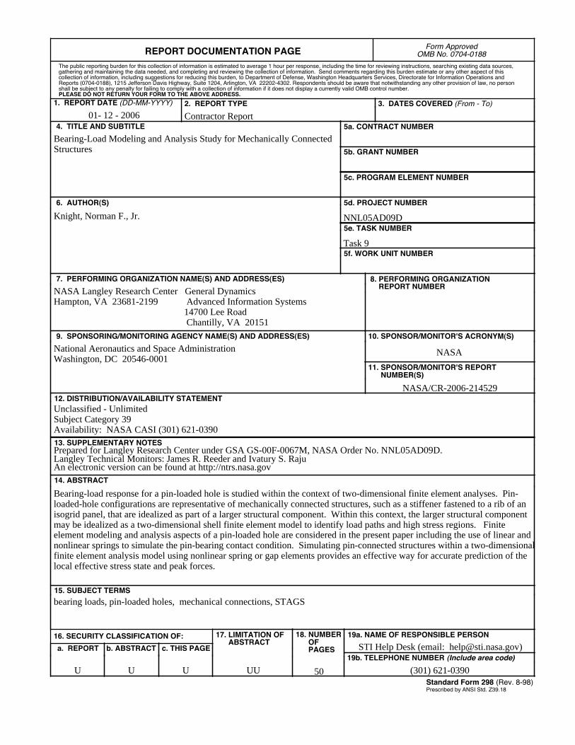
Bearing-load response for a pin-loaded hole is studied within the context of two-dimensional finite element analyses. Pin-loaded-hole configurations are representative of mechanically connected structures, such as a stiffener fastened to a rib of an isogrid panel, that are idealized as part of a larger structural component. Within this context, the larger structural component may be idealized as a two-dimensional shell finite element model to identify load paths and high stress regions. Finite element modeling and analysis aspects of a pin-loaded hole are considered in the present paper including the use of linear and nonlinear springs to simulate the pin-bearing contact condition. Simulating pin-connected structures within a two-dimensional finite element analysis model using nonlinear spring or gap elements provides an effective way for accurate prediction of the local effective stress state and peak forces.

15. SUBJECT TERMSbearing loads, pin-loaded holes, mechanical connections, STAGS

18. NUMBER OF PAGES

5019b. TELEPHONE NUMBER (Include area code)

(301) 621-0390

a. REPORT

U

c. THIS PAGE

U

b. ABSTRACT

U

17. LIMITATION OF ABSTRACT

UU

Prescribed by ANSI Std. Z39.18Standard Form 298 (Rev. 8-98)

3. DATES COVERED (From - To)

5b. GRANT NUMBER

5c. PROGRAM ELEMENT NUMBER

5d. PROJECT NUMBER

NNL05AD09D5e. TASK NUMBER

Task 95f. WORK UNIT NUMBER

11. SPONSOR/MONITOR'S REPORT NUMBER(S)

NASA/CR-2006-214529

16. SECURITY CLASSIFICATION OF:

The public reporting burden for this collection of information is estimated to average 1 hour per response, including the time for reviewing instructions, searching existing data sources, gathering and maintaining the data needed, and completing and reviewing the collection of information. Send comments regarding this burden estimate or any other aspect of this collection of information, including suggestions for reducing this burden, to Department of Defense, Washington Headquarters Services, Directorate for Information Operations and Reports (0704-0188), 1215 Jefferson Davis Highway, Suite 1204, Arlington, VA 22202-4302. Respondents should be aware that notwithstanding any other provision of law, no person shall be subject to any penalty for failing to comply with a collection of information if it does not display a currently valid OMB control number.PLEASE DO NOT RETURN YOUR FORM TO THE ABOVE ADDRESS.

1. REPORT DATE (DD-MM-YYYY)12 - 200601-