“because” without “cause”

* Dedicated to Peter Lipton (1954-2007). With thanks to Jeremy Butterfield.

“Because” without “Cause”:

The Uses and Limits of Non-Causal Explanation*

In this paper I deploy examples of non-causal explanations of physical phenomena as

evidence against the view that causal models of explanation can fully account for

explanatory practices in science. I begin by discussing the problems faced by Hempel’s

models and the causal models built to replace them. I then offer three everyday examples

of non-causal explanation, citing sticks, pilots and apples. I suggest a general form for

such explanations, under which they can be phrased as inductive-statistical arguments

incorporating plausible assumptions. I then show the applicability of this form to

explanatory practices in thermal physics. I explore the possibility that population genetics

provides a similar form of explanation, and offer a novel defence of the statistical

interpretation of population genetics proposed by Matthen and Ariew (2002). I close with

remarks concerning how, when faced with competing causal and non-causal explanations

of the same phenomenon, we can perform an Inference to the Best Explanation.

Jonathan

Birch, J. (2008). “Because” without “cause”: the uses and limits of non-causal explanation. BA thesis, University of Cambridge, 25 April 2008.

“BECAUSE” WITHOUT “CAUSE”

2

1. Introduction

The search for an account of explanatory practices in science has spanned six decades1.

One protagonist has cast a long shadow over all that has followed: Carl Hempel. Hempel

thought that to give a scientific explanation2 (henceforth: explanation) is to give an

argument. To Hempel, explanatory facts and laws serve as premises, from which we

conclude that the thing to be explained was (at least) to be expected given the premises,

and perhaps even followed from those premises with deductive certainty. Hempel took

the concept of a law for granted, and stipulated that there must always be at least one law

in an explanation. There was no explicit place for causation: causes may make their

effects expectable, but, if so, it’s the expectability that matters, not the causation. Few

would argue that Hempel’s models tell the whole story, and I am not among those few. I

do, however, contend that certain philosophers have been too quick in their attempts to

dismiss Hempel’s picture.

Causal models, proposed as a consequence of widespread criticism of Hempel, have

enjoyed popularity in recent years. Proponents of such models oppose the claim that

explanations are arguments, taking them to be an assemblage of relevant causes of the

thing to be explained. They aim to put the “cause” into “because” (Salmon 1977a, 215).

Adopting a causal model of explanation raises the possibility of non-causal explanations

(in which understanding intuitively appears to be reached without causes being given)

serving as potent counterexamples. Such counterexamples are the primary focus of this

paper.

1 Salmon (1989) suggests Hempel and Oppenheim (1948) as the starting point. 2 In this category, Hempel includes all explanations of empirical phenomena yielded by empirical inquiry

(Hempel 1965, 333). It is a deliberately broad definition. We might, however, wish to exclude from the

category, if they explain at all, mathematical proofs and philosophical arguments.


3

In this section, I discuss Hempel’s models and the causal models built to replace them3. I

highlight the significance of non-causal explanations as counterexamples to causal

models, and introduce the thesis I will defend. In Section 2, I offer three everyday,

intuitively plausible examples of non-causal explanations, citing sticks, pilots and apples.

I introduce a general form of non-causal explanation, in which contrastive questions are

answered by inductive-statistical arguments incorporating plausible assumptions. In

Section 3, I show how the conception of non-causal explanation established in Section 2

illuminates explanatory practices in thermal physics. In Section 4, I explore the

possibility that population genetics explains biological phenomena in a similarly

statistical, non-causal manner. I offer a novel defence of the statistical interpretation of

the theory as articulated by Mohan Matthen and André Ariew (2002) against the

criticisms of Frédéric Bouchard and Alex Rosenberg (2004, 2005). In Section 5, I

conclude that statistical explanations can be non-causal, that they can be arguments, and

that our explanatory practices are more heterogeneous than is often acknowledged. I close

with remarks concerning how, when faced with competing causal and non-causal

explanations of the same phenomenon, we can perform an Inference to the Best

Explanation.

1.1 Why reject Hempel?

Hempel’s two distinct models, as articulated in his 1965 landmark essay “Aspects of

Scientific Explanation”, he named the deductive-nomological (D-N) model and the

inductive-statistical (I-S) model. A proposed third model, the deductive-statistical, is

essentially the D-N model as applied to the explanation of a statistical law, and I will not

discuss this here.

A D-N explanation takes the form of a deductive argument. The explanatory work is done

by the premises, which must include at least one law. An explanation is any set of

premises that entail that the phenomenon-to-be-explained occurred. For example, if asked

3 My survey is purposely very limited in scope. Significantly, I omit discussion of unification accounts of

explanation (see Kitcher 1981).


4

to explain why Socrates was mortal, we could cite the particular fact that Socrates was a

man, together with the law that all men are mortal. A note on terminology: Hempel

(1965, 336) defines the term explanandum to refer either to the thing-to-be-explained (the

explanandum-phenomenon) or the sentence describing that thing (the explanandum-

sentence). An explanandum, to Hempel, can be a particular fact or a general law, though

the I-S model only deals in particular facts.

We cannot give a D-N explanation of a particular fact if the fact is not deducible from

any available information: perhaps it is fundamentally chancy, or appears chancy given

our current knowledge. But, as Hempel observed, this need not prevent explanation,

though the explanation offered might be less enlightening than the D-N ideal. His

solution, inspired by the D-N model, was the I-S model. Like a D-N explanation, an I-S

explanation is an argument. But it is inductive, not deductive. The premises, which must

contain a statistical law, do not entail the conclusion, but they do give it high inductive

support. The conclusion can be expected with a high probability (1965, 390).

Say, for example, we are observing a radioactive decay and record 100 decays in a

minute. We know the sample was of element X, and element X has a half-life λ such that

there was a 90% statistical probability that 100 decays would occur during the minute.

These considerations would have led us to expect 100 decays with high inductive

probability. They thereby explain why 100 decays did indeed occur. The higher the

inductive probability, the better the explanation, tending towards the ideal of 100%

inductive probability.

This example illustrates the two types of probability in an I-S explanation: the statistical

probability in the law, and the inductive probability conferred on the conclusion by the

premises. Hempel (1965, 387) suggests a deliberately vague finite-long-run relative

frequency interpretation of statistical probability4. On this view, for example, to say a

coin has a 50% probability of landing heads up is to say that, if you were to toss it a large

4 Hempel remained undecided as to his preferred interpretation of probability throughout his career

(Niiniluoto 1981, 143).


5

finite number of times, it would land heads-up 50% of those times. A statistical law need

not govern an irreducibly indeterministic process (and indeed coin tosses are not such a

process). The inductive probabilities, meanwhile, quantify our reasons to believe that the

explanandum was to be expected. This does not necessarily mean that these probabilities

are subjective. Hempel (1965, 385) follows Rudolf Carnap (1950) in maintaining that

there is some objective logic regarding what probability a set of premises confers on a

conclusion. Hempel’s 1965 conception of inductive probability is logical or epistemic.

Why is this not enough? Why can we not end the discussion here? The D-N and I-S

models are, alas, plagued with difficulties. Counterexamples to the D-N model are

plentiful, and the problems are more than technicalities: they appear to result from the

omission of causation from the theory. Say, for example, I plant a stick vertically in the

ground on a sunny day (example adapted from Bromberger 1965). I want to know why its

shadow has the length it has. A D-N explanation seems attractive: I can deduce the length

of the shadow from the length of the stick, the position of the sun and the laws of

trigonometry. So far so good. But what if I want to know why the stick has the length it

has? According to the D-N model, I can explain the stick’s length by deducing it from the

position of the sun, the length of the shadow and the laws of trigonometry. But this does

not seem to yield any understanding at all!

The D-N model faces a further problem of accounting for the intuitive distinction

between the explanatory role of events that are causally active and those that are causally

redundant. Jim, for example, is not pregnant. He is also male. Why is he not pregnant?

We can construct a D-N explanation as follows (example adapted from Salmon 1989,

50):

Jim takes the contraceptive pill. (particular fact)

No one who takes the pill gets pregnant. (law)

_________________________________________

Jim is not pregnant.


6

Intuitively, the premises here fail to explain the conclusion, but not because the argument

is unsound. Rather, the events we have cited are causally redundant. A correct

explanation should cite the cause that Jim is a man.

The I-S model inherits the weaknesses of the D-N model. It cannot distinguish the

explanatory roles of cause and effect and it cannot separate the causal from the causally

redundant. It also faces severe difficulties of its own. One problem arises from the

structure of inductive arguments. The addition of a new premise can wreck an inductive

argument; this is not the case with deductive arguments. Take the following inference:

Socrates is a man. (particular fact)

All men are mortal. (law)

Socrates is 8ft tall. (new premise)

_________________________________________

Socrates is mortal.

The new premise (though strange and presumably false) has not weakened the support

afforded to the conclusion. If my original premises are true, my conclusion cannot

possibly be false. Contrast this with a typical inductive argument (adapted from Salmon

1989, 54):

Jim has infection X. (particular fact)

Patients with infection X have a 90% chance of survival. (law)

=====================================5

Jim survives X.

This appears to be a good I-S explanation of why Jim survived. But new information can

change this:

5 I follow Hempel (1965, 383) in using a double line to separate premises from conclusion in an inductive

argument.


7

Jim has infection X.

Patients with X have a 90% chance of survival.

Jim has a new multi-drug resistant strain of X. (new premise)

Patients with multi-drug resistant X have a 10% chance of survival. (more specific law)

=====================================

Jim survives X.

In light of the new information, I cannot continue to maintain that my original argument

still explains Jim’s survival. My knowledge no longer suggests that Jim’s survival was to

be expected with high probability. How can the I-S model account for why we thought

the argument explained, but have now decided that it doesn’t? Hempel’s solution is to

impose a “requirement of maximal specificity” (1965, 400), an adaptation of Carnap’s

“requirement of total evidence” (Carnap 1950, 211-213)6. Take the following candidate I-

S explanation:

B

P (A|B) = 0.9 (Given B, there is a high probability of A occurring)

=====================================

A

This may or may not be an I-S explanation. It will not be an I-S explanation if the event

of type B is also an event of type B1, where B1 is a subset of B (that is, where B1 is a

more specific type of event), and we have formulated a law for the probability of A given

B1. In such a scenario, Hempel stipulates that an I-S explanation of A must invoke the

more specific law (1965, 400). This is what is meant by the “requirement of maximal

specificity.” Whether or not an argument qualifies as an I-S explanation is thus

relativized to what we know when we give it. Suppose that we don’t know of any law

more specific than that relating A and B. In such a case, the argument above provides an

I-S explanation. But if our knowledge situation had been different, and we’d been able to

6 The requirement of total evidence is inappropriate here. Evidence that the explanandum occurred (e.g. I

saw it) will not necessarily help show it was to be expected.


8

be more specific, the argument would not have been a correct explanation. It is therefore

wrong to speak of an “absolutely true” I-S explanation. To give an I-S explanation is not

to pick out any true causal or lawlike relations among real events. This admission is

unsatisfying for those with an intuition that the correctness of an explanation is

determined only by the world and not by the knowledge of the speaker giving the

explanation. As Alberto Coffa notes bluntly, “what, then, is the interest of I-S

explanations?” (1974, 158).

This is a question to which we shall return in Section 2. For the moment, note also that,

formally, the premises of an I-S argument must contain a statistical law, yet the use of the

term “law” for the relationship between the probabilities in our example may sound

implausible. For example, if we possessed fine-grained causal knowledge about Jim’s

particular immune system and the particular organisms infecting him, we’d end up

modifying our naïve probabilities considerably. The “law” does not appear to pick out

underlying causal relations in the world. How then, to interpret the “law”? We have

already conceded that I-S explanation is relativized to our current knowledge situation.

We can take “law” here to mean a formulated statistical generalization involving the right

kind of predicates7. It is merely the most specific generalization we have to hand; it is not

a claim about the causal mechanisms of the world. This may sound like an inappropriate

use of the word “law,” but scientists do on occasion use it in this sense. Take the Second

“Law” of Thermodynamics: under the statistical interpretation of the theory, this is in fact

a trend, and could (with negligibly small probability) be violated without any violation of

dynamical laws (e.g. Elga 2000). Yet it still seems apt to call it a law. In this paper, I will

retain Hempel’s terminology and take formulated statistical generalizations as “statistical

laws”.

A second problem with the I-S model lies in its demand for high probability. Can we

never explain the improbable? Michael Scriven (1959) offers the example of paresis, a

complication of syphilis, which develops in a small percentage of cases. Surely, for a case

7 The problem of identifying the right kind of predicates for laws still needs to be addressed (see Goodman

1983). I assume the generalizations in this paper involve appropriate predicates.


9

in which a syphilis patient contracts paresis, the syphilis explains the paresis, even though

the syphilis did not make the paresis probable. Hugh Mellor (1976) considers such

counterexamples inadequate for rejecting the high probability requirement for

explanation.8 A proponent of the high probability requirement can claim that the syphilis

could be an ingredient in an explanation, but would not in itself provide an explanation.

The syphilis raises the probability of the paresis, but an explanation should invoke

additional factors so that the final probability is made high. Finding factors that raise the

probability of the thing to be explained is an important but insufficient step in making the

probability high. In the paresis case, on Mellor’s view, there is no explanation.

Richard Jeffrey (1969) claims that, intuitively, we can explain improbable outcomes as

long as we know the law governing the stochastic process in question. If I toss a fair coin

five times (example adapted from Jeffrey 1969), and each time it turns up heads, this does

not defy explanation. If I know the coin was fair and that the probability of five heads,

though small, was non-zero (it is 1/32), this explains the outcome as well as we could

explain any outcome. To Mellor, however, an explanation of an explanandum, A, must

explain why A better than it would explain why not-A (1976, 327). One way to achieve

this is to insist that an explanation must show that A was to be expected with high

probability. Mellor offers the example of a game of bridge. If I am dealt cards from a

range of suits (the high probability outcome), the dealer could explain this by claiming

she was dealing fairly. If I am dealt cards of just one suit, could the dealer explain this by

claiming she was dealing fairly? It is certainly another possible outcome of a fair,

randomly dealt hand. But such an explanation would have explained a mixed-suit hand

much better than it explains a single-suit hand. In this improbable case, my suspicions are

aroused and a better explanation seems to be called for.

8 That is, with regard to the “good” explanations for which Mellor wants to account (1976, 241). The I-S

model seems to imply a sliding scale, where very low probability gives an “explanation,” but it is poor and

unsatisfactory. I hold that any scientific explanation should aim to be good, and so, like Mellor, seek to

account for “good” explanations. Where Mellor says “good explanation,” I say “explanation.”


10

Nonetheless, though the dealer’s explanation may not intuitively be the best possible

explanation, it is, if true, intuitively an explanation, so the I-S model does not wriggle out

of the counterexample so easily. Mellor claims that Jeffrey’s coin explanation (and the

dealer’s explanation of the single-suit deal) can intuitively explain something, but it

cannot do the explanatory work Jeffrey requires of it. Jeffrey claims that the fairness of

the coin explains why I got five heads in a row. Mellor suggests that the fairness actually

explains why I did not get five tails in a row (or did not get any other specific outcome

apart from the outcome obtained), since this latter event has high probability (31/32). It is

possible to explain such facts about the trial even while we cannot explain the more

“interesting” individual outcome (the five heads). The I-S model can evade Jeffrey’s

objection. It remains, however, a respect in which Hempel’s I-S proposal struggles to

match our intuitions.

1.2 Trouble for the causal model

A number of philosophers have in recent decades articulated causal models of

explanation as alternatives to the traditional Hempelian theory (see especially Humphreys

1981, Salmon 1984, Lewis 1986, Lipton 1990 and Woodward 2003)9. In this paper I will

consider David Lewis’s model as adapted by Peter Lipton, with the expectation that the

criticisms here raised will equally count against other models. For Lewis, a call for an

explanation (typically a why-question, a question beginning with “why”10) is a call for

information about the causal history of an event-to-be-explained. I will call this event the

explanandum event; I assume that all explanandum events are acceptable explananda

under Hempel’s permissive construal of the term. The explanation is not an argument.

The amount of information needed to satisfy the person calling for the explanation will

vary. The explanation will need to cite the right causes, and which causes these are will

9 Several philosophers offer causal accounts of explanation together with accounts of causation. I do not

here discuss causation, assuming that we can make sense of the idea of causal explanation without

requiring an account of causation to plug into it (see Lipton 2004, 31). 10 Perhaps not all calls for explanation can be put into this form (Salmon 1989, 137), but this is not the

concern of this paper.


11

be highly context-sensitive. For example, if asked “Why are you in Cambridge today?” it

would not appropriate to reply, “Because the Big Bang happened around 15 billion years

ago,” even though this answer does indeed give a cause. It can be particularly easy to

pick out the right causal information when the why-question is explicitly contrastive:

“Why A rather than B?” (Lipton 1990). Lipton terms A the fact and B the foil: the

contrasting event that did not occur. Causes of A that could otherwise have caused B are

rendered irrelevant. In these cases, we must cite causes that are events in the causal

history of A with absences of corresponding events in the causal history of B. Why did

Lewis go to Monash rather than to Oxford? Because Monash invited him (relevant

cause), and Oxford did not (corresponding absence) (Lipton 1990, 256).

Hempel hoped to give models that accounted for all scientific explanations. If the causal

model is to provide a credible alternative (enabling us to do away with Hempel’s

models), it must account for all such explanations, or at least a great deal of them. Thus

non-causal explanations, at least if they constitute a sizeable class of explanations,

threaten to undermine this model seriously. Lewis confronts this, and denies that we can

ever correctly give a non-causal explanation (1986, 221-224). I endorse Lewis’s

criticisms but disagree with his conclusion. Lewis does not consider the type of candidate

non-causal explanation I will discuss: that is, statistical explanation. Lipton is more

conciliatory: some explanations, he concedes, are non-causal, but there is still an

“overwhelming preponderance” of causal explanations (Lipton 1990, 248). Lipton

suggests, for example, that philosophical arguments and mathematical proofs can offer

non-causal explanation. I will not explore this possibility: even if they do offer

explanation of a sort, it is not, I suggest, scientific explanation of physical phenomena,

and this is my concern here. I aim to show that large classes of contrastive why-questions

pertaining to physical phenomena can be answered wholly non-causally. I will articulate

some everyday examples of non-causal explanation (including Lipton’s), and argue that

similar explanations are often provided by science, notably in thermal physics, and

perhaps in population genetics.


12

Figure 1: The sphere of possible stick orientations

2. Everyday cases

2.1 Spinning sticks: realizing the mean

This example is adapted from Peter Lipton (1990,

248). It will set the general format for the

examples subsequently discussed. I throw a large

number of sticks into the air. They all spin rapidly

as they fall. I take a photo of the sticks in mid-air

(the camera is on a tripod; it is exactly horizontal),

and observe that, in the photo, the sticks are

predominantly closer to the horizontal than to the

vertical.

Here is the explanation: I have no reason to

believe that, for any one stick, any orientation is any more likely to be realized in the

photo than any other. I assume that, for the average stick, all orientations are roughly

equally likely to be realized (if any individual sticks are biased, the biases will roughly

cancel out). There are more ways for a stick to be oriented closer to the horizontal than

there are ways for the stick to be oriented closer to the vertical. Figure 1 shows this. Let

every pair of diametrically opposite points on the sphere’s surface represent one possible

orientation for the stick. The shaded area represents those orientations that are closer to

the horizontal. The shaded area on the sphere’s surface is greater than the non-shaded

area. It was therefore to be expected that most sticks would be oriented nearer the

horizontal.

What question does this explanation answer? It seems to me that, if we state the why-

question explicitly, it should be contrastive. It is: “Why did I observe most sticks to be

closer to the horizontal, rather than observing most sticks to be closer to the vertical?”

This contrastive question rules out answers like “because I took a photo” or “because I

threw them.” Such answers do cite causes of the explanandum event, but they are not


13

relevant causes, because they would also have occurred in the causal history of the foil,

had it occurred.

The explanation is an argument to the effect that the explanandum event was to be

expected. Though Lipton does not describe it as such, this is surely a great example of

statistical explanation. Explanation is achieved through knowledge of the options

available to each stick, knowledge of the states (of orientation) that are accessible to it.

Of the two contrasting outcomes, the majority-horizontal outcome is statistically more

probable than the majority-vertical outcome. It is the expected outcome, or the mean

outcome, and it is expectable with high probability.

The explanation is non-causal. This, at least, is Lipton’s claim, which he justifies with an

assertion that “geometrical facts cannot be causes” (2004, 32). Here he presumably

adopts Lewis’s (1973) doctrine that the correct relata of a cause-effect relation are events

not facts, or the view that mathematical objects cannot be causes (Baker 2005, 234).

Mellor (1995) argues that the relata of a cause-effect relation are facts, so this may (at a

stretch) be a cause of controversy with the spinning stick example. Others may object that

there is a hidden relevant cause: whatever event brought the geometrical facts into being

(the Big Bang, presumably). I think, however, that the explanation remains non-causal

irrespective of whether we take the view that geometrical facts cannot be causes. The

reason is that, even if geometrical facts are causes of the outcome, they are causes that

would feature equally in the causal history of the foil, had it occurred. There is no

corresponding absence of geometrical facts in the causal history of not-B, where B is the

event of most sticks appearing closer to the vertical.

Having observed that the explanation is a statistical argument, we might wonder whether

it fits Hempel’s I-S model for explanatory statistical arguments. If it does, it does so as

follows:

(1) The sticks spun in the air.

(2) For each spinning stick, P (horizontal orientation) > ½


14

=====================================

Most sticks were closer to the horizontal than to the vertical.

The premise (2) is a statistical law that confers high probability on the conclusion. The

probabilities in the “law” do not follow from any irreducible indeterminacy in the

process: if we’d known everything there was to know about the causes influencing the

sticks at a fine-grained level, we could have refined the probabilities. Rather, as in the

case of infection X (see Section 1), the argument quantifies our reasons to expect certain

possible outcomes, based on our knowledge situation. The statistical law is tacitly

underwritten by an assumption which, given our current knowledge situation, we find

plausible: that every orientation was roughly equally likely. The requirement of maximal

specificity is fulfilled, because we did not know of any causes affecting the outcome (e.g.

air currents). I conclude that the explanation is inductive-statistical. I also observe that, as

Lipton notes, it is “a lovely explanation” (1990, 248).

2.2 The Israeli Air Force: regression to the mean

This example is from Daniel Kahneman and Amos Tversky, and is documented by

Lipton (2004, 32). Trainee pilots in the Israeli air force were strongly praised after

performing well, and strongly criticized after performing poorly. It was observed that the

pilots tended to improve after receiving criticism, but tended to get worse after receiving

praise. What explains this behaviour? Perhaps criticism was more effective than praise in

causing improvement. But there is another explanation.

It is based on the idea that a particular middling level of performance was the mean, or

expected performance. But we need to make a plausible assumption that performance was

a random variable distributed roughly symmetrically about this mean (the following

argument fails for seriously skewed distributions). Let us say they follow a normal (bell-

shaped) distribution. It can then be argued that it was to be expected that the praised

pilots would follow an unusually good performance with a poorer performance (a

performance closer to the mean), and it was to be expected that the criticized pilots would


15

follow an unusually poor performance with a better one (also a performance closer to the

mean).

Again we can put the question in a specifically contrastive form: “Why did most pilots

perform worse after praise, rather than better?” (A corresponding question could be posed

with regard to the criticized pilots.) Again, the answer we are considering is statistical

and is an argument. And again, it can be put into the form of an I-S explanation. Let x0

represent each pilot’s initial performance, X represent the variable of subsequent

performance, and μ represent the mean performance.

(1) For all the praised pilots, x0 > μ.

(2) If x0 > μ, P (X<x0) > ½

=====================================

Most praised pilots subsequently performed at a level below x0.

As in the spinning stick case, the probabilities do not follow from the irreducible

indeterminacy of a pilot’s performance. This will be influenced by a huge range of factors

(whether they concentrate, whether they went out drinking the night before, and so on).

The argument quantifies the extent to which the outcome was to be expected given our

knowledge situation. Maximal specificity is satisfied: we do not know anything about the

pilots, other than that they were above average to begin with. Again, the statistical law is

underwritten by a plausible assumption: that, in these circumstances, the performances

roughly fit the right kind of probability distribution. We could obviously give a parallel

explanation for the subsequent performance of the criticized pilots.

Ultimately, this is a pleasing real-life illustration of a spinning-stick-style explanation.

The only difference is that the fact and foil are defined relative to some fact previously

obtained (initial performance), which must meet a certain criterion (viz. being above

average). I follow Lipton in claiming that this too is “a lovely explanation” (2004, 32).

The role previously played by geometrical facts in Section 2.1 is played in this example

by facts about the normal distribution over all possible levels of performance. This


16

example is particularly interesting in so far as the I-S explanation competes with a

plausible causal explanation (that criticism was more effective in causing improvement).

2.3 Apples: standard deviation from the mean

This example is adapted from Denis Walsh (2007, 283). Take three varieties of apple:

Braeburn, Jonagold and Pippin. In mean mass, they rank as follows: Braeburn > Jonagold

> Pippin. But in standard deviation (a measure of spread, how much they tend to deviate

from the mean), they rank: Pippin > Jonagold > Braeburn. Braeburns are biggest on

average, while Pippins are most variable on average.

There are five markets nearby, and each market contains five fruit stalls. From each fruit

stall I buy ten apples of each variety (that is, 750 apples overall; I like apples). I make an

assumption that the mass of the apples I picked varied randomly according to roughly the

same probability distribution at all stalls. I was not, for example, deliberately picking out

the heavy ones at certain stalls, or the ripe ones or the pretty ones. For each sample of 50

per variety from each market I calculate the mean mass of each variety. I discover that,

for four of the markets, Braeburn had the highest mean mass, and, for the odd one out, the

Jonagolds had the highest mean mass. I am not surprised. The order “Braeburn >

Jonagold > Pippin” has been reflected in the number of markets where each variety came

out heaviest.

Next, I calculate the mean mass of each variety from each sample of ten per variety from

each stall. Note that these batches are much smaller. This time I discover that Braeburns

(unsurprisingly) come out heaviest for 14 stalls, but (surprisingly) the Pippins come out

heaviest in seven, while the Jonagolds only come out heaviest in four. The number of

stalls where each variety came out heaviest goes: “Braeburn > Pippin > Jonagold”. The

rank order has changed.

This is explained by the high standard deviation of the Pippins. They were smaller on

average overall, but their high standard deviation meant it was to be expected that fluke


17

heavy Pippins would skew the sample mean of individual batches, pushing it above that

of the other varieties fairly often. This effect was more marked in the smaller apple

batches, because in a small batch a fluke heavy Pippin skews the sample mean more

severely than in a large batch (and is less likely to be cancelled out by a fluke small

Pippin).

This boils down to a similar explanation to the two given above. It is different in so far as

knowledge of standard deviations is needed. We ask: “Why did the rank deviate from the

predicted rank when the sample size was decreased to ten, rather than when the sample

size was 50?” The answer will be a statistical argument that can be framed in accordance

with the I-S model as follows:

(1) Sample sizes of ten and 50 were taken.

(2) P (Rank deviates more in a smaller sample size) is high.

=====================================

The rank deviated more from the predicted rank when the sample size was ten rather than

when the sample size was 50.

The explanation is non-causal, because the facts about standard deviations, if they are

causes at all, would have been causes in the causal history of the foil, had it occurred.

Note also that, yet again, the statistical law is underwritten by a plausible assumption. I

would know it to be false if I knew that I or someone else had (perhaps subconsciously)

rigged the sampling in certain ways. Perhaps I let the mass of certain apples influence my

decision to choose them, or perhaps the fruit sellers have a strange apple-size cartel in

operation. In the absence of knowledge of any such circumstance, it sounds plausible to

say that the mass of the sampled apples varied randomly under the same probability

distribution at each stall.

2.4 Where from here?


18

I have discussed three plausible everyday cases of non-causal explanations. I have shown

that they are statistical in nature, and that they can be phrased as I-S arguments. In 2.2,

we also saw how a real postulated non-causal explanation can conflict with a real

postulated causal explanation. So far, there is not much to concern advocates of causal

models. Like Lipton, they can concede that, in a handful of exceptional cases, there can

be lovely non-causal explanations. As we will soon see, however, this handful typifies a

form of explanation into which huge classes of explanations fit.

We are now in a position to answer Coffa’s question: what is the interest of I-S

explanations, when they are relativized to our knowledge? The answer, I think, is that

they turn the unexpected into the expected. Without applying knowledge of the geometry

of spheres, it would seem very strange that the sticks so often appeared closer to the

horizontal. An intuitive response to the spinning stick observation is surprise: shouldn’t I

have expected about half to be closer to the horizontal, given that there are only two

options for each stick and I can’t help but be epistemically indifferent towards the two?

The I-S explanation tells me otherwise: given the known facts and the assumptions I find

plausible, I really should have expected the observed outcome. The I-S argument explains

by transforming the unexpected into the expected, the surprising into the unsurprising. It

does not matter that the premises of the argument fail to pick out true causal relations in

the world. Nancy Cartwright (1983, 47-53) observes that the strict truth of a claim about

an experimental setup is not a pre-requisite for its use in a good explanation of the

outcome. A claim we suspect would prove strictly false given fine-grained detail of the

setup, such as Snell’s Law, or our spinning stick generalization, can still explain.

We can also, I think, put aside Jeffrey’s objection, at least in these specific cases. Can

there be explanation without high probability? Let us specifically ask this question with

respect to the spinning sticks: if most sticks had come out closer to the vertical, could the

sphere of possible orientations still have explained why this occurred, rather than most

sticks appearing closer to the horizontal? Intuitively, I suggest the answer is that it could

not. We have two options: accept Jeffrey’s intuition and deny that the sphere of

orientations can explain anything, or accept that this is a case where high probability


19

really does explain. Having already claimed that the explanation is “lovely,” I of course

take the latter route.

A common feature of all the non-causal explanations I have discussed is the role of

plausible assumptions. We may ask: what makes them plausible? It is not that we are

convinced of their strict truth. The answer, I think, lies in the principle of indifference:

the view that, when faced with a range of possible outcomes, we should assign them

equal probability unless we know of something to choose between them. The principle

has met with strong criticism (e.g. Howson and Urbach 2006, 262-272), but it seems that

the “plausible assumptions” involved in our examples employ appropriate applications of

something like a principle of indifference. What makes these applications appropriate? It

is that we have specified the possible options accessible to the sticks/pilots/apple samples

in as much fine-grained detail as our knowledge allows. Knowing the stick orientation

options, but knowing no better, we postulated that all were roughly equally likely to be

occupied by the average stick. Knowing the performance options available to the pilots,

but knowing no better, we postulated the performances varied randomly under a roughly

symmetric probability distribution. Knowing there were twenty-five stalls, but knowing

no better, we postulated that the mass of the apples followed roughly the same probability

distribution at every stall.

Coffa ends his 1974 paper with a discussion of whether philosophers can tell scientists

what explains and what doesn’t. I think they can, but only if the proffered scientific

explanation clashes with very strong everyday intuitions we all possess. As I have shown,

I-S explanations relativized to a knowledge situation do not fall into this category. I

suggest, then, that if they exist in science, we should defer to scientists and concede that

they really are scientific explanations. I will now show that they do exist.


20

Figure 2

Figure 3

3. Thermal physics

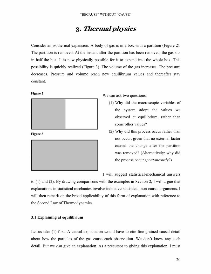
Consider an isothermal expansion. A body of gas is in a box with a partition (Figure 2).

The partition is removed. At the instant after the partition has been removed, the gas sits

in half the box. It is now physically possible for it to expand into the whole box. This

possibility is quickly realized (Figure 3). The volume of the gas increases. The pressure

decreases. Pressure and volume reach new equilibrium values and thereafter stay

constant.

We can ask two questions:

(1) Why did the macroscopic variables of

the system adopt the values we

observed at equilibrium, rather than

some other values?

(2) Why did this process occur rather than

not occur, given that no external factor

caused the change after the partition

was removed? (Alternatively: why did

the process occur spontaneously?)

I will suggest statistical-mechanical answers

to (1) and (2). By drawing comparisons with the examples in Section 2, I will argue that

explanations in statistical mechanics involve inductive-statistical, non-causal arguments. I

will then remark on the broad applicability of this form of explanation with reference to

the Second Law of Thermodynamics.

3.1 Explaining at equilibrium

Let us take (1) first. A causal explanation would have to cite fine-grained causal detail

about how the particles of the gas cause each observation. We don’t know any such

detail. But we can give an explanation. As a precursor to giving this explanation, I must


21

spell out some of the terms it invokes. I will discuss classical thermal physics and set

aside the quantum formulation, as do most discussions of the philosophy of thermal

physics, though the quantum version is widely applied by practising scientists.

If we take the gas molecules to be classical-mechanical point particles bouncing around

in a box, a snapshot at any moment of these particles would capture each particle with a

particular position and momentum. All the particles together constitute a system. The

snapshot shows the microstate of the system. On this view, the system can adopt a

continuous range of microstates, with the constraint that the total energy of the system

must be conserved. This range includes even wildly implausible microstates, such as the

particles lining up to lap the edges of the container, or all the particles gathering into a

tiny ball in the centre. All these possible microstates constitute a phase space: an abstract

space in which each point represents one accessible microstate. This can be pictured as a

vast set of possible systems, of which only one is the actual system. We can overlay the

phase space with a probability distribution, assigning probabilities to every region. This

set of systems, spanning a phase space, overlain by a probability distribution, is the

ensemble. For our gas, it is conventional wisdom to say all phase space regions of equal

volume are equally likely to be occupied (this assumption is controversial, see below):

the resultant ensemble is the micro-canonical ensemble11. The actual system will only

realize one microstate at any one instant, so the evolution of the system over time can be

pictured as a dot touring around the phase space.

So here is the explanation. Large numbers of microstates are very similar to each other.

There are certain regions of the phase space that correspond to the same macroscopic

properties. We can say the macroscopic property supervenes on regions of the phase

space. Let us visualize this in terms of gas volume. The gas is observed to occupy the

entire container (Figure 3; let us say the gas is coloured and the container is transparent,

so this is very easy to observe). It need not do this. It could occupy half the container, or a

11 There are two other important ensembles, the canonical and the grand canonical, which I do not discuss

here; I assume the explanatory practices are the same in all cases. See Gibbs (1905) for the coining and

defining of these ensembles.


22

quarter, or a tiny section. But these macroscopic possibilities are not of equal probability.

The gas occupying the whole container is an option that is realized at the vast majority of

points in the phase space. The gas occupying only a tiny section of its container can be

realized only by a tiny region of the phase space. As far as we know, all regions of the

phase space are equally likely to be occupied by the actual system when we make our

observations. It is therefore to be expected with high probability that, when we observe it,

the system will be in the region of the phase space corresponding to it occupying the

whole volume of the container.12

I have not yet used the term entropy: in statistical thermodynamics, this beautiful word

denotes a measure of phase space volume. Entropy, S, is equal to klogW, where W is a

number of microstates, or a volume of the phase space, and k is the Boltzmann constant.

It follows that the gas occupying the entire volume of the container, which is the state

corresponding to the largest region of the phase space, is the highest entropy state. The

highest entropy state is the one that is to be expected, owing to the above considerations.

Mathematicians have devoted a great deal of attention to one aspect of this form of

explanation. It was assumed above that all regions of the phase space of equal phase

space volume are equally likely to be occupied by the system when we make an

observation. Recall that we can visualize the actual system as a dot moving through the

phase space. There is a tension between these ideas. Ludwig Boltzmann postulated that,

given infinite time, the system would in fact pass through all points of the phase space

equally often, and that this justifies our assignment of probabilities (Sklar 1993, 44). This

is the ergodic hypothesis. But why should the system explore all areas of the phase space

equally? It could get stuck in certain stable regions of microstates. The ergodic

hypothesis has thus spawned ergodic theory: the enterprise of trying to show it is correct.

In any case, even if Boltzmann was right, long-run relative frequencies over infinite time

do not strictly imply anything about what we should expect in observations carried out

12 Such explanations are found in many scientific texts: for example, Chandler (1987, 54-62), Nash (1974,

23-26). For alternative philosophical expositions, see Albert (2000, 35-51), van Fraassen (1980, 161-167).


23

over finite time. Infinite long-run relative frequency is thus the wrong interpretation of

probability for I-S explanation (Hempel 1965, footnote 10).

I do not think this problem damages the explanatory power of the explanation. Rather, it

is part of an attempt to find some underlying dynamical process that will provide

supplementary understanding. Recall that, in the spinning stick case, we assumed that, for

the average stick, all orientations were roughly equally likely to be observed, even though

fine-grained causal detail might have given us cause to alter our probabilities. The

assignment of probabilities was plausible, and explanatorily permissible. The same goes

here. Even if we believe that our idealized assumptions about probabilities over the

microstate ensemble might well turn out to be strictly false given further evidence, they

can still serve our explanatory needs. In our current knowledge situation, it is permissible

and plausible to assume that every microstate is equally likely to be occupied.13

It is worth dwelling on the comparison between thermodynamic processes and spinning

sticks. In both cases, the explanation is an argument that shows the explanandum was to

be expected with high probability14. In the thermodynamic case, the probabilities are

typically very high. The probability of the body of gas not filling the container to any

observable extent can be estimated and even calculated to be negligible. As with the

spinning sticks, the probabilities we cite are based on our knowledge of the possibilities

available. Intuitively, this knowledge of possibilities appears to rationalize our choice of

probabilities. We can put the gas explanation in I-S form as follows15:

(1) For the ensemble of microstates for this system, the probability of the body of gas

filling the container is very high.

13 Cartwright (1983, 153-155) defends a similar point. Sklar (1973) turns the point on its head. Arguing

against narrow Hempelian conceptions of explanation, he suggests that, since real scientists want to

supplement their knowledge with ergodic theory, some explanation must be possible over and above the

basic statistical explanation. My aim is to point out that the basic explanation still explains. 14 Strevens (2000) stresses the crucial importance of the high probability requirement in thermal physics. 15 Clark (1990, 165) also suggests that statistical mechanics offers I-S explanations.


24

=====================================

The gas was observed to fill the container.

There is a slight disanalogy with the stick case. The possible orientations of the stick

depend on geometrical facts, which cannot be explanatorily relevant causes. The possible

microstates of a system in thermal equilibrium depend on the total energy available to the

system, the degrees of freedom available to the molecules, and (in the more modern and

versatile quantum formulation) on the discrete energy levels of the molecules. Why can’t

these facts be relevant causes? To be able to say definitively that they are not, we need to

specify the foil in the why-question very carefully. The foil cannot be a different

macroscopic result (e.g. volume) emerging from a different microstate ensemble. We

need to require that the ensemble is the same in the fact and foil cases. In short, if we

want a wholly non-causal answer, the question must be specified as follows: Why did the

macroscopic variables of the system adopt the values we observed at equilibrium, rather

than some other values, for this particular microstate ensemble? If we leave out the final

clause, the answer could be part causal, part non-causal, if we allow that the parameters

defining the ensemble might be causes of the equilibrium properties.

This modified question may seem obscure. Do physicists and chemists really ask this

type of question? They do, for both predictive purposes and explanatory purposes. The

microscopic parameters (total energy, degrees of freedom, energy levels) that define the

ensemble are measured by spectroscopy, the values of the macroscopic variables are

calculated, and the observations tend to match the expected values to a high degree of

accuracy.

Lawrence Sklar (1993, 151) notes that this is a “curious” form of explanation. It is

presupposed that the system is at equilibrium, and presupposed that the system has

particular micro-properties. We then argue that, given all this, it was to be expected that

the system displayed particular macro-properties. I reply that the curiosity Sklar identifies

results from the fact that the explanation is a non-causal explanation. I also suggest that it

is not that curious. As we have seen, similar considerations explain in everyday cases.


25

3.2 Explaining the approach to equilibrium

Now I turn to question (2): why did this process occur rather than not occur, given that no

external factor caused the change after the partition was removed? There is a short

answer: regression to the mean.16 It was to be expected that a system not realizing its

mean properties (not filling its container) would come to do so, as indeed any isolated

system out of equilibrium will tend to move towards it. We can borrow the schema from

Section 2.2, and again visualize the process in terms of volume. Let V represent the

macroscopic variable volume (in physical space), v0 represent the initial volume, and μ

represent the mean volume (where the mean is calculated by averaging over the phase

space).

(1) For the gas, at time t0, v0 < μ.

(2) If v0 < μ, then at time t0+δ, P (V>v0) is high.

=====================================

V>v0 at time t0+δ

We can thus explain why the gas expands in the small time interval after the partition is

removed, and at every subsequent interval until V= μ. As in the case of the Israeli pilots,

there is no cause, no push: the explanation is non-causal. Facts about the probability

distribution over the phase space take on the role played by geometrical facts in the

spinning stick case.

One might reply, like Sklar (1993, 282), that this is unacceptably quick. It is plainly

untrue that every microstate is equally likely to follow from a certain initial microstate.

The system starts out at a certain point in the phase space and is constrained by

dynamical laws to follow a subsequent path. Particles cannot jump instantaneously from

one side of the box to the other: the laws of physics impose a strong restriction. But note

16 For alternative expositions of the basic idea, see Price (1996, 30) and Albert (2000, 51-62). For a

physicist’s perspective, see Nash (1974, 29-36).


26

that it is also plainly untrue that an individual pilot is equally likely to perform at any

level following a good performance. Surely each such pilot is more likely to perform at a

fairly high level: the causes that caused the initial good performance may well still be

active (for example: quick reflexes, experience, technique), and the initial good

performance itself might boost morale and cause a future good performance. But we

dismissed all these unknown causal factors when offering a statistical explanation

relativized to our knowledge. As in the equilibrium case, a lot of mathematicians have

spent a lot of time looking for understanding of the underlying dynamical relations in the

approach to equilibrium. This does not imply, however, that the simple explanation can’t

explain. As in the equilibrium case, the assumption that all microstates are equally likely

to be occupied is a plausible assumption that facilitates an explanation through which we

transform the surprising into the unsurprising.

3.3 Outside the box

Statistical mechanics can of course explain far more than isothermal gas expansion inside

a box. Clear analogies can be drawn with diffusion and osmosis, and notable explanatory

work has been done with regard to chemical equilibria and rates of reaction. The famous

Second Law of Thermodynamics states that not only will certain experimental setups

move towards the highest entropy state, but so will the entire universe in any physical

process. It is thought to be a statistical law, not a dynamical law. How, then, does it result

from the statistics? According to conventional wisdom (e.g. Price 1996, 37), the answer

in a nutshell is that we are living in a giant approach to equilibrium. The Big Bang was a

low-entropy initial condition a long way from equilibrium for the system it created, and it

is thus to be expected that the universe will keep heading towards that equilibrium. The

Big Bang was like removing the partition in Figure 2, and we are still undergoing the

long transition to Figure 3.

The Second Law highlights the extraordinarily wide applicability of statistical-

thermodynamical explanation. We can explain many “spontaneous” events, especially

approaches to equilibrium: from the expansion of a gas in a box to the cooling of the


27

Earth. As we have seen, the explanation is non-causal, and rather like the examples in

Section 2. There is a vast class of non-causal explanations.


28

4. Population genetics

Mohan Matthen and André Ariew, in a provocative 2002 paper, defend the claim that

explanation in population genetics shows striking similarities to the type of explanation in

thermal physics we saw in Section 3. Their motivation is a troubling problem in

philosophy of biology: how to account for the “predictive fitness” values of traits (that

feature in the equations of population genetics) in terms of the individual-level causal

properties that go into “vernacular fitness,” a creature’s relative “adaptedness” to its

environment (central to basic expositions of the theory of evolution). Their solution:

claim that population genetics does not explain by appeal to vernacular fitness at all. My

aim in this section is not to survey the large and growing literature on statistical and

dynamical interpretations of natural selection. Rather, I briefly describe the

Matthen/Ariew picture; and I suggest a novel interpretation of the interpretation, under

which the explanations can be formulated as non-causal I-S arguments17. I then evaluate

the strength of the analogy between explanatory practices in thermal physics and

population genetics, with particular reference to the criticisms of Frédéric Bouchard and

Alex Rosenberg (2004, 2005).

4.1 The Matthen/Ariew picture

According to Matthen and Ariew (2002), the trait frequency changes we observe in

populations are to be explained by appeal to the predictive fitness values of traits

(henceforth: trait fitnesses), and the mathematical equations of population genetics that

feature them. These trait fitnesses will be assigned on the basis of a range of facts, which

might include information about trait frequencies in the past, or considerations of the

competitive advantage of organisms with the trait (2002, 78)18. The trait fitnesses are “a

17 Hempel (1965, 391-392) himself suggests that genetics provides exemplary I-S explanations. 18 Walsh, Lewens and Ariew (2002) offer a similar picture, with a significant difference. They claim trait

fitnesses are averages of (causal) propensities in individual organisms: “individual fitnesses.” Can we

justify a propensity interpretation of individual fitness? How can we know these propensities? I leave aside

these issues here.


29

measure of evolutionary change not a cause” (2002, 56). Yet they do play an

indispensable explanatory role (Matthen, personal communication). If some why-

questions about trait frequencies can be answered solely by trait fitnesses and

mathematical formulae, the explanation will, it seems, be non-causal. Population genetics

will explain by tracking statistical trends and estimating the probability of an

explanandum’s occurrence, given information about the state of the population prior to

the explanandum event.

An analogy between population genetics and thermal physics is central to the

Matthen/Ariew thesis: “natural selection, like thermodynamic change of state, is a time-

asymmetric statistical trend instantiated by populations” (2002, 80). We saw in Section 3

how no causal process (no “push”) need be cited in order to explain why gas in half a box

will expand to fill it. We can show the expansion was expectable, and our reasons for

believing it was expectable are not causes. In this section, I entertain the suggestion that

the analogy is sufficiently close such that population genetics explanations follow the

form discussed in Section 3.

I suggest that population genetics explains via arguments to the effect that, given

information about a population at time t0, subsequent patterns of growth in the frequency

of traits were to be expected with high probability. Where does natural selection come

into this? When the observed trait frequency growth pattern matches exactly that

predicted by the fitness, we call the trend “pure natural selection”. The observed pattern

may deviate from expectation to some extent in a finite population, and we call the

statistical deviation “drift”.

Consider a thought experiment, adapted from Matthen and Ariew (2002, 72), to which we

can apply this kind of explanation. I put $100 in investment fund A, and $100 into

investment fund B. I observe the money build up for a few years, and observe that A

grows consistently at 6% while B grows consistently at 2%. I can start to make

predictions about how the funds will fare in the future. Ten years later I find that nearly

all my money is now in the A fund. It has grown far more than the B fund. But a quick


30

calculation reveals that this finding was to be expected with high probability given the

steady growth rates I knew about ten years earlier. The A/B ratio has shifted towards the

expected value, and this is just a trend, not a causal process. No one has donated money

to my A fund, and I haven’t moved any money around. Roughly speaking, Matthen and

Ariew want us to say A-dollars have been favoured by selection over B-dollars. If the

actual value is exactly the expected value for this time, we can call the trend “pure

selection”. If the actual value has deviated from the expected value, we call the trend

“selection plus drift”. In either case, the explanation is non-causal.

We can formalize the sort of I-S explanations population genetics may offer. First, let us

set the question: Why did trait A increase in frequency in population P between time t0

and time t0+δ, rather than decrease, given all known information about P at t0? The

known information has to be held constant across fact and foil so as to isolate the non-

causal explanatory work than can be done, just as we held the ensemble constant in

Section 3, and held the geometrical facts constant in Section 2.1. This is the simplest sort

of question we might ask. Population genetics also explains, for example, variation in the

rate of frequency increase. In more complex cases, more complex laws will replace

premise (2), but the general form of explanation should still apply. The explanation is

non-causal, provided that trait fitnesses cannot be causes. Let wi represent all relevant

trait fitness values, and f2 and f1 represent final and initial frequencies of trait A

respectively:

(1) wi

(2) If wi, P (f2>f1) is high.

=====================================

The trait frequency of A increased.

4.2 Disanalogy

Bouchard and Rosenberg (2004, 2005) aim to drag population genetics down to Earth.

The Matthen/Ariew picture, they argue, offers explanations “that pass only the lowest of


31

stringency tests” (2004, 709). Good explanations in population genetics must be causal,

and the causal relations must be at the level of individual organisms. Bouchard and

Rosenberg do not aim to attack explanations in thermal physics, but they claim the

explanatory practices we studied in Section 3 cannot apply in population genetics. Their

argument is that a disanalogy results from the fact that explanations in thermal physics

irreducibly explain at the level of ensembles. Their meaning is not clear here. They refer

to an “ensemble of particles” (2004, 702), which differs from my usage of the term. They

could mean “system of particles”, or they could mean “ensemble of microstates”. The

former is more appropriate. Statistical mechanics takes probability distributions over the

phase space, but the macroscopic physical properties it purports to explain (volume in our

example) are properties of the system of gas particles in the actual world.

Bouchard and Rosenberg suggest we simply cannot explain such properties in terms of

the behaviour of particles: we must appeal to the “mysteries of the second law” (2004,

702). This is false. As we saw in Section 3, we explain by appeal to the possible

microstates open to the particles. The explanation is not causal, and leaves room for more

understanding, but it is not mysterious either. Bouchard and Rosenberg’s objection to

these explanations is that:

Within any given region of space and range of momentum values for any

one particle, the position and momentum of the particle can take up to a

continuum of values. If the earlier “smaller” number of arrangements

[microstates] compatible with a given distribution is infinite in number,

and the later, larger “number” of arrangements is also infinite in number,

we cannot appeal to differences in the number of arrangements on which

given distributions supervene to explain the increase in entropy that the

second law reports. (2004, 702)

This argument fails for two reasons. First, the number of microstates is not infinite under

the quantum picture, and this is the preferred formulation in many contexts. Second, even

in the classical context, we can overcome the problem of all infinities being equal in size,


32

for we can integrate probabilities over regions of the phase space. Bouchard and

Rosenberg’s claim about our inability to compare sizes of continuous ranges of values

generalizes, absurdly, to any continuous probability

distribution (so that no range of values in a normal

distribution is any more likely than any other) and

even to Cartesian space (Figure 4). Which is bigger:

A or B? If Bouchard and Rosenberg are correct,

nobody knows! They both contain a continuum of

points in space.

Why does this matter? It re-opens the possibility that statistical trends in thermal physics

are not irreducible to individual-level causal processes. Rather, they do correspond to an

underlying causal process, but, in the absence of fine-grained knowledge about this

process, we can still explain the trend. This was the argument of Section 3. Having

demystified statistical-mechanical explanation, we can use its plausibility to argue that, if

similar explanations are indeed offered by biologists, they can explain without reference

to causes.

Bouchard and Rosenberg proceed to argue that phenomena in population genetics can

and must be explained by individual-level causal explanations, in a way in which (on

their view) phenomena in thermal physics cannot be explained. They offer coin tossing

by way of analogy (2004, 705). Say I toss a coin ten times, and record six heads. I am

surprised: I was expecting five heads. Let us assume that nothing about the processes

involved is irreducibly indeterministic. Rather, for every toss the outcome followed

necessarily from the initial conditions and the forces acting on the coin. According to

Bouchard and Rosenberg, I fail to give an adequate explanation if I claim that, though

five heads was the smart bet, the six heads can be explained as being statistical deviation

from the expected value. I should instead say that something about the initial conditions

and the forces in play caused the observed outcome, and to explain the outcome I should

state that cause (2004, 706). Likewise, even if I observe five heads, my claiming it was

the smart bet is not enough. I should say that something about the initial conditions and

Figure 4


33

forces explains the five heads, even though the causes (and hence the explanation) is in

practice epistemically inaccessible. When a causal explanation is available “in principle”

(2004, 708), statistical explanation is not good enough.

We can see why this might not be the case by returning to the thermal physics analogy. In

thermal physics, we believe there is some true causal story about how a body of gas

spreads from half a box to the whole box. If we knew it, we could explain our

observations. But this causal story is to all intents and purposes inaccessible. We look for

a statistical explanation not because the causal history is not there, but because we do not

know it; and perhaps also because we want a different type of understanding:

expectability, not knowledge of causes. We use our current knowledge and plausible

assumptions to construct an explanation relativized to that knowledge. Biologists often

find themselves in a similar predicament. They know enough to estimate trait fitnesses

for traits in a population, but not nearly enough to piece together reliably the individual-

level processes that caused the evolutionary change. And even if they could look for an

individual-level story, it might not provide the type of understanding they seek (Matthen

and Ariew 2005, 363).

4.3 High probability

This much must be conceded to Bouchard and Rosenberg: we must avoid an account that

suggests we can, from a position of near-total ignorance, explain everything. Intuitively,

explanations that invoke extreme random drift are unsatisfying. And there are alternatives

to drift: I may have misjudged the trait fitnesses, or my whole theory may be wrong

(Bouchard and Rosenberg 2004, 708-709). How can we choose between the alternatives?

Say that, for two traits A and B in a population P at ratio 50/50 at time t0, the trait

fitnesses show it was to be expected that the A/B frequency ratio would converge to

72/28 by some long-run limit-time, t1. In fact, I observe the ratio 15/85. I could hardly

have been more wrong. Can I explain my observation by citing drift? Surely not. This

observation is a prompt to look for a miscalculation, or a flaw in the theory. There must

be a limit on the explanatory power of statistical arguments in which drift is cited.


34

I propose that a suitable cut-off point for explanation is offered by Hempel’s high

probability requirement (see Section 1.1, and Hempel 1965, 390). Suppose that, for traits

A and B as described above, the observed A/B ratio actually becomes 68/32 at t1. There

was drift from the expected value. If I ask why the ratio increased rather than decreased, I

can give a statistical explanation. If I ask more specifically why the ratio was between

60/40 and 80/20, rather than in some other region, I can explain this too. But as I narrow

down the explanandum it will become less and less expectable. Plainly, if I ask why the

observed frequency was exactly 68/32 and not 72/28, I will not be able to argue that the

explanandum was to be expected with high probability. I will have to conclude that this

explanandum cannot be explained by a statistical argument. But I can still offer

explanations of the first two sorts. In the case of the 15/85 ratio, the high probability

requirement blocks all attempts at statistical explanation.

4.4 The bad news

I have so far stressed the viability of the thermal physics analogy in spite of the attack by

Bouchard and Rosenberg. Nonetheless, there remains a crucial limitation on the analogy.

In Section 3, I stressed the importance of the assumption that every microstate is equally

likely to be occupied. Only with this assumption in place could we use phase space

regions as good guides to the probability of particular observations obtaining. Here, we

take trait fitnesses as good guides to the probability of particular trait frequencies

obtaining: but why? There is no ensemble (as defined in Section 3) in population

genetics. There is no “counting the microstates” procedure to calculate the mean

outcome. The statistical probabilities in population genetics do not arise from considering

possibilities and applying a principle of indifference. So why are we prepared to believe

them in explanations? I contend that, for population genetics to produce plausible

statistical arguments, we must maintain that the probabilities in the theory supervene on

individual-level causal properties. Recall our economics example: the 6% and 2% growth

rates (analogous to trait fitnesses) were taken as good guides to future growth: but why?

Because the trend picks out a causal process: the investment is on the way up because the


35

companies concerned are doing well – a causal matter of fact. Probabilities in population

genetics supervene on individual-level causal properties19, while probabilities in thermal

physics need not do so (though ergodic theory hopes to show that, at least in a cautious

treatment of statistical mechanics, they do).

If trait fitness supervenes on individual-level causal properties, we might at least wonder

whether trait fitness itself can be a cause. Intuitively, a coin’s bias can be a cause despite

its supervenience on fine-grained properties of the structure of the coin; gas pressure can

be a cause despite its supervenience on the fine-grained properties of a gas; and perhaps

mental states can be causes despite their supervenience on brain states (see especially

Shapiro and Sober 2007). This raises a possibility that cannot be analogously sustained in

the case of the gas expansion: the possibility that the theory, while dealing only with

trends at the level of populations, explains via population-level causes. This is the view

defended in a number of recent papers (e.g. Reisman and Forber 2005, Millstein 2006,

Shapiro and Sober 2007). I will not survey their arguments in detail20. The key claim is

that we can change natural selection outcomes by manipulating trait fitnesses21, and we

can change drift outcomes by manipulating population sizes, since drift tends to be more

marked in a smaller population. So, applying a manipulationist criterion for causation22

(see Woodward 2003), natural selection and drift are causal processes.

I concede that the non-causal statistical interpretation of natural selection faces

difficulties. Nonetheless, it is relevant to our discussion of non-causal explanation. I

19 Walsh et al. (2002, 460) accept this: see footnote 18 in this paper. 20 Note that one hurdle they must overcome is Kim’s (1993) argument for epiphenomenalism (that is, the

view that supervenient properties are causally inefficacious). 21 Suppose, in a population of moths, a subpopulation has the trait “peppered colouration,” which provides

camouflage against predators. If their tree environment was a different colour (e.g. black), all else being

equal, their reproductive success would have been different. Fodor (2008) attacks the coherence of using

counterfactuals and “all else being equal” clauses in biology. 22 In short: an event X causes an event Y iff there exists a possible intervention on X that would be

associated with a change in Y, or in the probability of Y (Shapiro and Sober 2007). Strevens (2007)

criticizes this account.


36

submit that the apparent importance of statistical explanations in population genetics, the

continuing debate over plausible non-causal interpretations of these explanations, and the

possibility of formulating such explanations as I-S arguments, counts against the view

that the causal model is all there is to explanation. I admit that it is far from established

that evolutionary explanations are non-causal explanations, and far from established that

the analogy between thermal physics and population genetics holds. The analogy,

however, is promising, and is sufficiently robust to withstand the criticisms of Bouchard

and Rosenberg. The debate continues, but the possibility that population genetics explains

non-causally remains open.


37

5. Conclusion

5.1 The best explanation?

The form of non-causal explanation I have articulated in this paper is not a suitable form

of explanation to plug into an Inference to the Best Explanation (IBE): the sort of

inference, which, according to many recent accounts (e.g. Lipton 2004) lies at the heart of

scientific practice. The conclusion of an Inference to the Best Explanation is that the best

explanation is true. Under my account, the statistical explanations I have discussed

cannot be conclusions of such an inference for a simple reason: they are not known to be

true. Recall Coffa’s objection: I-S explanations are relativized to our current knowledge.

As I have been emphasizing throughout this paper, the examples we have seen are

examples of such relativized explanations.

This does not mean that non-causal explanations are of no use to scientists who seek true

explanations via IBE. We have seen that they transform the surprising into the

unsurprising, and can, on occasion (see Section 2.2), remove the grounds we thought we

had for inferring the truth of a causal explanation of the explanandum concerned. This is

the role of statistical explanations in IBE: they block causal explanations.

I suggest that, to be the “best explanation,” a causal explanation must explain something

that cannot be explained non-causally. Before it is rational to believe that criticism causes

improved performance in Israeli pilots, it is necessary to generate some phenomenon that

criticism can explain and statistics cannot: perhaps, for example, small changes in the

intensity of the criticism would be found to correlate very well with small variations in

subsequent performance. Before it is rational to accept that some as yet unknown factor

causally explains the behaviour of a gas, it is necessary to find some aspect of its

behaviour that cannot be explained statistically. Non-causal explanations are not

incompatible with IBE. They do not claim to be true, and they can guide our IBE

practices.


38

5.2 Closing comments

Large classes of explanations are non-causal. These explanations are statistical arguments

that show the explanandum was to be expected with high probability. Thermal physics is

a ripe source of such non-causal statistical explanations, often overlooked in the

literature. But there are everyday cases too, and it is in these cases that the power of non-

causal explanation is most compelling. Moreover, population genetics offers up a second

very large class of explanations where non-causal explanation might be more prevalent

than is generally acknowledged. Attempts to draw parallels between population genetics

and thermal physics are promising, but so far the picture of natural selection and drift as

causal processes is yet to be refuted.

The Lewis/Lipton causal model of explanation tells far from the whole story. In cases of

clear contrastive why-questions, where the causal answer, if there was one, should have

been clear, we have found no causal explanation and a satisfying non-causal explanation.

I doubt that the explanations I have discussed can be brought under any umbrella of

causal explanation. If this is the case, causal models in general cannot tell the whole story

about our explanatory practices. I have suggested that Hempel’s I-S model may be able to

account for the non-causal explanations. Though Coffa and Jeffrey’s objections to the I-S

model as a complete account of all statistical explanation are plausible, they do not block

the applicability of Hempel’s model to the non-causal explanations I have discussed.

I do not, however, rule out the possibility that other models may suffice for this purpose.

In particular, I have not discussed Philip Kitcher’s (1981) influential unification account

of explanation. Michael Strevens (2004) hints at the possibility of a radically new causal

model able to accommodate statistical explanations in thermal physics: the “kairetic”

account. I await the full articulation of this model with both interest and scepticism. In the

meantime, I will settle for the straightforward conclusion that Lewis was wrong: there are

scientific explanations of physical phenomena that are not causal, and our explanatory

practices are less uniform than he suggests.


39

Bibliography

Albert, D. Z. (2000), Time and Chance. Cambridge, MA: Harvard University Press.

Baker, A. (2005), "Are There Genuine Mathematical Explanations of Physical

Phenomena?" Mind 114: 223-238.

Bouchard, F., and A. Rosenberg (2004), "Fitness, Probability and the Principles of

Natural Selection", British Journal for the Philosophy of Science 55: 693-712.

Brandon, R., and G. Ramsey (2007), "What’s Wrong with the Emergentist Statistical

Interpretation of Natural Selection and Random Drift", in M. Ruse and D. L. Hull

(eds.), The Cambridge Companion to Philosophy of Biology. Cambridge:

Cambridge University Press, 66-85.

Bromberger, S. (1965), "An Approach to Explanation", in R. J. Butler (ed.), Analytical

Philosophy. Vol. 2. Oxford: Basil Blackwell, 72-105.

Carnap, R. (1950), Logical Foundations of Probability. Chicago: Chicago University

Press.

Cartwright, N. (1983), How the Laws of Physics Lie. Oxford: Clarendon Press.

Chandler, D. (1987), Introduction to Modern Statistical Mechanics. New York: Oxford

University Press.

Clark, P. (1990), "Explanation in Physical Theory", in D. Knowles (ed.), Explanation and

Its Limits. Cambridge: Cambridge University Press, 155-177.

Coffa, J. A. (1974), "Hempel’s Ambiguity" Synthese 28: 141-163.

——— (1977), "Probabilities: Reasonable or True?" Philosophy of Science 44: 186-198.

Elga, A. (2000), "Statistical Mechanics and the Asymmetry of Counterfactual

Dependence", Philosophy of Science 68: 313-324.

Fetzer, J. H. (1992), "What's Wrong with Salmon's History: The Third Decade",

Philosophy of Science 59: 246-262.

Fodor, J. (2008), "Against Darwinism", Mind and Language 23: 1-24.

Gibbs, J. W. (1905), Elementary Principles in Statistical Mechanics. [Online] Available:

http://www.aip.org/history/gap/PDF/gibbs.pdf [Accessed: 21/04/08]

Goodman, N. (1983), Fact, Fiction and Forecast. 4th ed. Cambridge, MA: Harvard

University Press.


40

Hempel, C. G. (1965), "Aspects of Scientific Explanation", in Aspects of Scientific

Explanation and Other Essays in the Philosophy of Science. New York: Free

Press, 331-496.

——— (1968), "Maximal Specificity and Lawlikeness in Probabilistic Explanation",


Hempel, C. G., and P. Oppenheim (1948), "Studies in the logic of explanation",


Hitchcock, C. (1999), "Contrastive explanation and the demons of determinism", British

Journal for the Philosophy of Science 50: 585-612.

Howson, C., and P. Urbach (2006), Scientific Reasoning: The Bayesian Approach. 3rd ed.

Chicago: Open Court.

Humphreys, P. (1981), "Aleatory explanations", Synthese 48: 225-232.

——— (1989), The Chances of Explanation: Causal Explanation in the Social, Medical

and Physical Sciences. Princeton: Princeton University Press.

Jeffrey, R. C. (1969), "Statistical Explanation vs. Statistical Inference", in N. Rescher

(ed.), Essays in Honor of Carl G. Hempel. Dordrecht: D. Reidel, 104-113.

Kim, J. (1993), Supervenience and Mind. Cambridge: Cambridge University Press.

Kitcher, P. (1976), "Explanation, Conjunction, and Unification", Journal of Philosophy

73: 207-212.

——— (1981), "Explanatory Unification", Philosophy of Science 48: 507-531.

Lewis, D. K. (1973), "Causation", Journal of Philosophy, 70: 556-67.

——— (1986), "Causal Explanation", in Philosophical Papers. Vol. 2. Oxford: Oxford

University Press, 214-240.

Lipton, P. (1990), "Contrastive Explanation", in D. Knowles (ed.), Explanation and Its

Limits. Cambridge: Cambridge University Press, 247-266.

——— (2004), Inference to the Best Explanation. 2nd ed. London: Routledge.

Matthen, M., and A. Ariew (2002), "Two Ways of Thinking about Fitness and Natural

Selection", Journal of Philosophy 119: 55-83.

——— (2005), "How to Understand Casual Relations in Natural Selection: Reply to

Rosenberg and Bouchard", Biology and Philosophy 20: 355-364.

Mellor, D. H. (1976), "Probable Explanation", Australasian Journal of Philosophy 54:


41

231-241.

——— (1995), The Facts of Causation. London: Routledge.

Millstein, R. (2006), "Natural Selection as a Population-Level Causal Process", British

Journal for the Philosophy of Science 57: 627-653.

Nash, L. K. (1974), Elements of Statistical Thermodynamics. 2nd ed. Mineola: Dover

Publications.

Niiniluoto, I. (1982), "Statistical Explanation", in G. Floistad (ed.), Contemporary

Philosophy: A New Survey. Vol. 2. The Hague: Nijhoff, 157-187.

Price, H. (1996), Time's Arrow and Archimedes' Point: New Directions for the Physics of

Time. New York: Oxford University Press.

Railton, P. (1978), "A Deductive-Nomological Model of Probabilistic Explanation",


Reisman, K., and P. Forber (2005), "Manipulation and the Causes of Evolution",


Rosenberg, A., and F. Bouchard (2005), "Matthen and Ariew’s Obituary for Fitness:

Reports of Its Demise Have Been Greatly Exaggerated", Biology and Philosophy

20: 343-353.

Ruben, D.-H. (1990), Explaining Explanation. London: Routledge.

Salmon, W. C. (1977a), "An "At-At" Theory of Causal Influence", Philosophy of Science

44: 215-224.

——— (1977b), "Hempel's Conception of Inductive Inference in Inductive-Statistical

Explanation", Philosophy of Science 44: 179-185.

——— (1984), Scientific Explanation and the Causal Structure of the World. Princeton:

Princeton University Press.

——— (1989), Four Decades of Scientific Explanation. Pittsburgh: University of

Pittsburgh Press.

Scriven, M. (1959), "Explanation and Prediction in Evolutionary Theory", Science 130:

477-482.

——— (1975), "Causation as Explanation", Noûs 9: 3-16.

Shapiro, L. A., and E. Sober (2007), "Epiphenomenalism - The Dos and the Don'ts", in P.

Machamer and G. Wolters (eds.), Thinking about Causes: From Greek


42

Philosophy to Modern Physics. Pittsburgh: University of Pittsburgh Press, 235-

264.

Sklar, L. (1973), "Statistical Explanation and Ergodic Theory", Philosophy of Science 40:

191-212.

——— (1993), Physics and Chance. Cambridge: Cambridge University Press.

Sober, E. (1983), "Equilibrium explanation", Philosophical Studies 43: 201-210.

——— (2000), Philosophy of Biology. 2nd ed. Boulder: Westview Press.

——— (2001), "The Two Faces of Fitness", in R. S. Singh, C. B. Krimbas, D. B. Paul

and J. Beatty (eds.), Thinking about Evolution: Historical, Philosophical, and

Political Perspectives. Cambridge: Cambridge University Press, 309-322.

Strevens, M. (2000), "Do Large Probabilities Explain Better?" Philosophy of Science 67:

366-390.

——— (2004), "The Causal and Unification Accounts of Explanation Unified –

Causally", Noûs 38: 154-179.

——— (2007), "Essay review of Woodward, Making Things Happen", Philosophy and

Phenomenological Research 74: 233-249.

van Fraassen, B. C. (1980), The Scientific Image. Oxford: Clarendon Press.

Walsh, D. M. (2007), "The Pomp of Superfluous Causes: The Interpretation of

Evolutionary Theory", Philosophy of Science 74: 281-303.

Walsh, D. M., T. Lewens, and A. Ariew (2002), "The Trials of Life: Natural Selection

and Drift", Philosophy of Science 69: 452-473.

Woodward, J. (2003), Making Things Happen: A Theory of Causal Explanation. Oxford:

Oxford University Press.

“because” without “cause”

Documents