bedrosian et al., (2004) - university of alberta

www.elsevier.com/locate/tecto

Tectonophysics 385 (2004) 137–158

Geophysical images of the creeping segment of the

San Andreas fault: implications for the role of crustal

fluids in the earthquake process

P.A. Bedrosiana,*, M.J. Unsworthb, G.D. Egbertc, C.H. Thurberd

aDepartment of Earth and Space Sciences, University of Washington, Seattle, WA 98195, USAbDepartment of Physics, University of Alberta, Edmonton, Alberta, Canada T6G 2J1

cCollege of Ocean and Atmospheric Sciences, Oregon State University, Corvallis, OR 97331, USAdDepartment of Geology and Geophysics, University of Wisconsin, Madison, WI 56706, USA

Received 17 September 2002; received in revised form 15 July 2003; accepted 10 February 2004

Available online 2 July 2004

Abstract

High-resolution magnetotelluric (MT) studies of the San Andreas fault (SAF) near Hollister, CA have imaged a zone of high

fluid content flanking the San Andreas fault and extending to midcrustal depths. This zone, extending northeastward to the

Calaveras fault, is imaged as several focused regions of high conductivity, believed to be the expression of tectonically bound

fluid pockets separated by northeast dipping, impermeable fault seals. Furthermore, the spatial relationship between this zone

and local seismicity suggests that where present, fluids inhibit seismicity within the upper crust (0–4 km). The correlation of

coincident seismic and electromagnetic tomography models is used to sharply delineate geologic and tectonic boundaries. These

studies show that the San Andreas fault plane is vertical below 2 km depth, bounding the southwest edge of the imaged fault-

zone conductor (FZC). Thus, in the region of study, the San Andreas fault acts both as a conduit for along-strike fluid flow and a

barrier for fluid flow across the fault. Combined with previous work, these results suggest that the geologic setting of the San

Andreas fault gives rise to the observed distribution of fluids in and surrounding the fault, as well as the observed along-strike

variation in seismicity.

D 2004 Elsevier B.V. All rights reserved.

Keywords: San Andreas fault; Calaveras fault; Magnetotellurics; Hollister; Seismic tomography

1. Introduction

Large strike-slip faults such as the San Andreas fault

(SAF) and North Anatolian fault have generated some

0040-1951/$ - see front matter D 2004 Elsevier B.V. All rights reserved.

doi:10.1016/j.tecto.2004.02.010

* Corresponding author. Now at: GeoForschungsZentrum—

Potsdam, Telegrafenberg, Potsdam D-14473, Germany. Tel.: +49-

331-288-1258; fax: +49-331-288-1235.

E-mail address: [email protected] (P.A. Bedrosian).

of the most destructive earthquakes of the last century.

A range of geological and geophysical studies in the

last 20 years have greatly improved our understanding

of the earthquake rupture process. These faults often

show significant spatial and temporal variations in

seismic behavior. For example, the San Andreas fault

is characterized by a creeping central segment, with

locked segments to the north and south, each having

ruptured just once during the historical record (Allen,

P.A. Bedrosian et al. / Tectonophysics 385 (2004) 137–158138

1968). The mechanisms controlling which segments

creep and which are locked are not well understood. It

is likely that the composition of the wall rocks has some

influence on seismic behavior. However, it has also

been proposed that seismic behavior may be controlled

by a fluid network within the fault zone. The ability of

overpressured fluids to facilitate brittle failure at re-

duced effective normal stresses was first suggested by

Rubey and Hubert (1959). Irwin and Barnes (1975)

suggested the San Andreas fault creeps in regions

where the Great Valley sequence (GVS) is cut by the

fault. According to this hypothesis, the Franciscan

complex is viewed as a source of aqueous fluids

(derived from metamorphic reactions) which migrate

into the San Andreas fault along the boundary between

the Franciscan complex and the Great Valley sequence.

Recent studies, however, suggest that the role of

fluids in faulting is more complicated than previously

thought. High fluid pressure is an important compo-

nent of the current debate concerning the strength of

the SAF (Zoback et al., 1987; Mount and Suppe,

1987; Scholz, 2000; Townend and Zoback, 2000). In

order to explain the apparent weakness of the SAF,

complex models with spatially and/or temporally

varying fluid pressure distributions are also called

upon. Models by Sleep and Blanpied (1992) and

Byerlee (1993) are based upon periodic fluid flow in

the fault zone throughout the earthquake cycle. In

such models, fluids are believed to enter the highly

permeable and porous fault zone following an earth-

quake. Over time, shearing, creep compaction, and

mineralization form low-permeability seals which

isolate the fault zone from the surrounding country

rock. Pore pressures then increase until rupture (an

earthquake) occurs and the cycle begins again.

These models may explain both the apparent

weakness of the SAF and its along-strike seismic

variability. They suggest that significant permeability

contrasts exist across the fault and that isolated,

overpressured pockets of fluid might occur within

the fault zone. The existence of these features is best

examined through a combination of drilling and

surface-based geophysical exploration.

Magnetotellurics (MT) is a geophysical technique

for imaging subsurface resistivity structure using nat-

ural electromagnetic waves. Because the resistivity of

crustal rocks is strongly influenced by fluid content,

MT is well suited to imaging the presence and distri-

bution of fluids within major fault zones. In the last

decade, a number of MTstudies have helped define the

geometry and nature of the San Andreas fault zone in

central California. Mackie et al. (1997) and Unsworth

et al. (1999) imaged a narrow, low porosity San

Andreas fault at Carrizo Plain, within the southern

locked zone which last ruptured in the 1857 Fort Tejon

earthquake. In contrast, magnetotelluric studies at

Parkfield, within the transition zone between the creep-

ing segment to the north and the locked segment to the

south, imaged a prominent fault-zone conductor (FZC)

extending to 3–4 km depth and attributed to 9–30%

saline fluids (Unsworth et al., 1997, 2000). The first

detailed MT study of the creeping central segment was

described by Bedrosian et al. (2002) and imaged an

extensive zone of enhanced electricalconductivity be-

tween the San Andreas and Calaveras faults, that

extended to midcrustal depths beneath the SAF. Seis-

mic tomography studies in the same location imaged a

coincident zone of low Vp and high Vp/Vs, suggesting a

fluid-rich region beneath and to the northeast of the

SAF (Thurber et al., 1997). In this paper, a more

detailed analysis of the MT data is presented. In

combination with the seismic data, the geometry and

distribution of fault-zone fluids are examined, and their

implications for fault mechanics discussed.

2. Magnetotelluric data collection and analysis

The MT data were acquired in 1999 along two

profiles that crossed the San Andreas and Calaveras

faults (Fig. 1). The northern (Paicines) line crossed

both the SAF and Calaveras faults about 20 km

southeast of Hollister within the southern end of the

Hollister Trough. The southern (Bear Valley) line

crosses the same faults at the northern edge of the

Pinnacle Volcanic formation, some 20 km further to

the southeast. Continuous MT profiling, with electric

dipoles laid end to end, was used within several

kilometers of the major faults, and allows the problem

of static shifts to be partially overcome. Vertical

magnetic field variations were also recorded every

500–1000 m in the vicinity of the faults. The MT data

were synchronously recorded with two ElectroMag-

netic Instruments MT-24 systems at two sites (one on

each profile) to allow for the removal of incoherent

noise. This remote referencing technique was first

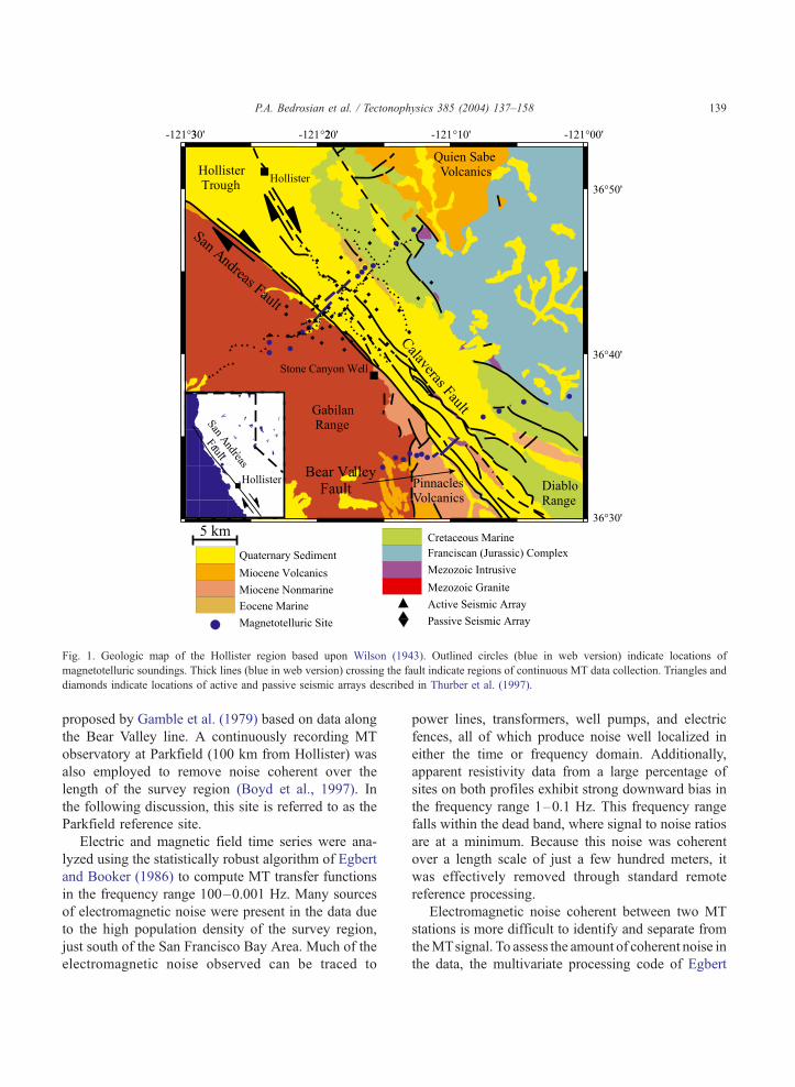
Fig. 1. Geologic map of the Hollister region based upon Wilson (1943). Outlined circles (blue in web version) indicate locations of

magnetotelluric soundings. Thick lines (blue in web version) crossing the fault indicate regions of continuous MT data collection. Triangles and

diamonds indicate locations of active and passive seismic arrays described in Thurber et al. (1997).

P.A. Bedrosian et al. / Tectonophysics 385 (2004) 137–158 139

proposed by Gamble et al. (1979) based on data along

the Bear Valley line. A continuously recording MT

observatory at Parkfield (100 km from Hollister) was

also employed to remove noise coherent over the

length of the survey region (Boyd et al., 1997). In

the following discussion, this site is referred to as the

Parkfield reference site.

Electric and magnetic field time series were ana-

lyzed using the statistically robust algorithm of Egbert

and Booker (1986) to compute MT transfer functions

in the frequency range 100–0.001 Hz. Many sources

of electromagnetic noise were present in the data due

to the high population density of the survey region,

just south of the San Francisco Bay Area. Much of the

electromagnetic noise observed can be traced to

power lines, transformers, well pumps, and electric

fences, all of which produce noise well localized in

either the time or frequency domain. Additionally,

apparent resistivity data from a large percentage of

sites on both profiles exhibit strong downward bias in

the frequency range 1–0.1 Hz. This frequency range

falls within the dead band, where signal to noise ratios

are at a minimum. Because this noise was coherent

over a length scale of just a few hundred meters, it

was effectively removed through standard remote

reference processing.

Electromagnetic noise coherent between two MT

stations is more difficult to identify and separate from

theMTsignal. To assess the amount of coherent noise in

the data, the multivariate processing code of Egbert


(1997) was employed. This makes use of multiple

channels at multiple sites to determine the coherency

of signal and noise within an array of synchronously

recorded sites. With an array consisting of the Parkfield

reference site and one or more sites from the Hollister

survey area, we identified two coherent noise sources

within the array. The first, prominent from3 to 0.5Hz, is

coherent between sites in the Hollister area but inco-

herent with the Parkfield reference site, and hence

separable from theMTsignal. The second noise source,

between 0.1 and 0.003 Hz, is coherent among all

channels and sites within the array, and thus cannot be

separated from the data. Egbert et al. (2000) attributed

this noise to the BayArea Rapid Transit system. For our

purposes, the average power of this artificial EM signal

is 10–20 dB less than theMTsignal power and does not

strongly bias MT transfer function estimates.

2.1. Dimensionality

The inversion of magnetotelluric data is greatly

simplified if a two-dimensional (2D) analysis can be

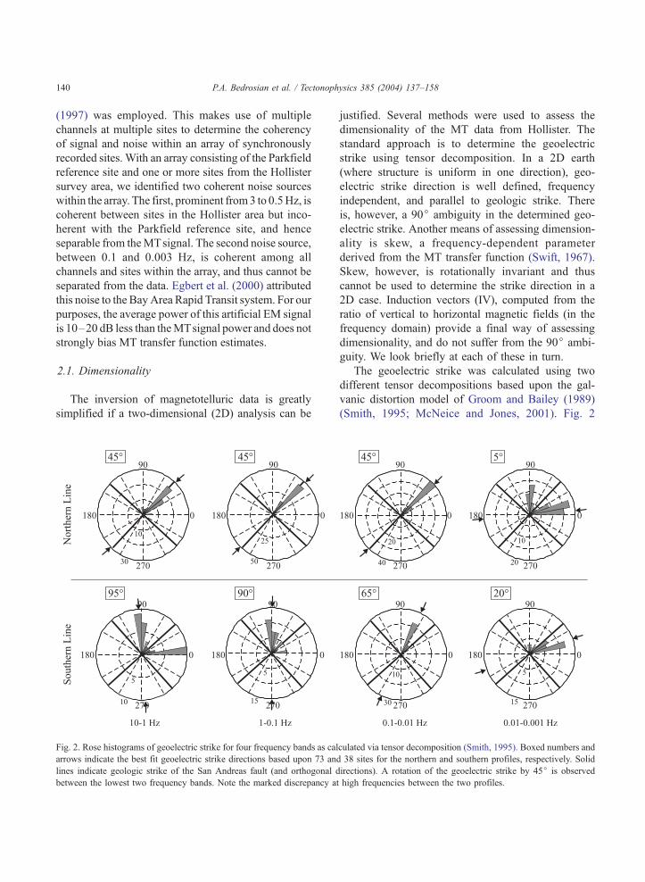
Fig. 2. Rose histograms of geoelectric strike for four frequency bands as cal

arrows indicate the best fit geoelectric strike directions based upon 73 an

lines indicate geologic strike of the San Andreas fault (and orthogonal d

between the lowest two frequency bands. Note the marked discrepancy a

justified. Several methods were used to assess the

dimensionality of the MT data from Hollister. The

standard approach is to determine the geoelectric

strike using tensor decomposition. In a 2D earth

(where structure is uniform in one direction), geo-

electric strike direction is well defined, frequency

independent, and parallel to geologic strike. There

is, however, a 90j ambiguity in the determined geo-

electric strike. Another means of assessing dimension-

ality is skew, a frequency-dependent parameter

derived from the MT transfer function (Swift, 1967).

Skew, however, is rotationally invariant and thus

cannot be used to determine the strike direction in a

2D case. Induction vectors (IV), computed from the

ratio of vertical to horizontal magnetic fields (in the

frequency domain) provide a final way of assessing

dimensionality, and do not suffer from the 90j ambi-

guity. We look briefly at each of these in turn.

The geoelectric strike was calculated using two

different tensor decompositions based upon the gal-

vanic distortion model of Groom and Bailey (1989)

(Smith, 1995; McNeice and Jones, 2001). Fig. 2

culated via tensor decomposition (Smith, 1995). Boxed numbers and

d 38 sites for the northern and southern profiles, respectively. Solid

irections). A rotation of the geoelectric strike by 45j is observed

t high frequencies between the two profiles.

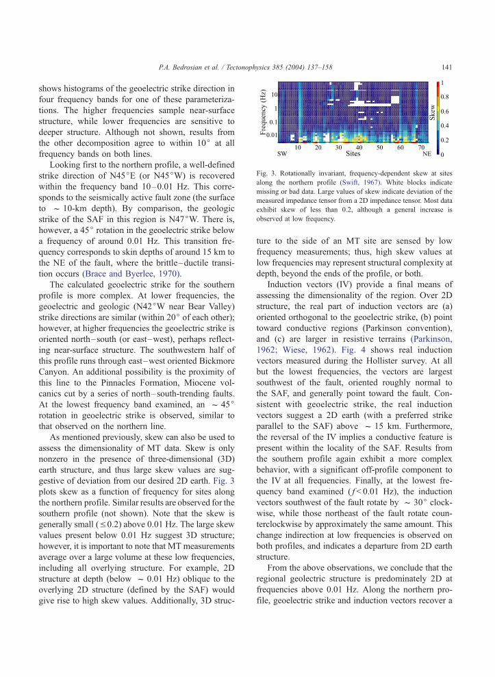
Fig. 3. Rotationally invariant, frequency-dependent skew at sites

along the northern profile (Swift, 1967). White blocks indicate

missing or bad data. Large values of skew indicate deviation of the

measured impedance tensor from a 2D impedance tensor. Most data

exhibit skew of less than 0.2, although a general increase is

observed at low frequency.


shows histograms of the geoelectric strike direction in

four frequency bands for one of these parameteriza-

tions. The higher frequencies sample near-surface

structure, while lower frequencies are sensitive to

deeper structure. Although not shown, results from

the other decomposition agree to within 10j at all

frequency bands on both lines.

Looking first to the northern profile, a well-defined

strike direction of N45jE (or N45jW) is recovered

within the frequency band 10–0.01 Hz. This corre-

sponds to the seismically active fault zone (the surface

to f 10-km depth). By comparison, the geologic

strike of the SAF in this region is N47jW. There is,

however, a 45j rotation in the geoelectric strike below

a frequency of around 0.01 Hz. This transition fre-

quency corresponds to skin depths of around 15 km to

the NE of the fault, where the brittle–ductile transi-

tion occurs (Brace and Byerlee, 1970).

The calculated geoelectric strike for the southern

profile is more complex. At lower frequencies, the

geoelectric and geologic (N42jW near Bear Valley)

strike directions are similar (within 20j of each other);however, at higher frequencies the geoelectric strike is

oriented north–south (or east–west), perhaps reflect-

ing near-surface structure. The southwestern half of

this profile runs through east–west oriented Bickmore

Canyon. An additional possibility is the proximity of

this line to the Pinnacles Formation, Miocene vol-

canics cut by a series of north–south-trending faults.

At the lowest frequency band examined, an f 45jrotation in geoelectric strike is observed, similar to

that observed on the northern line.

As mentioned previously, skew can also be used to

assess the dimensionality of MT data. Skew is only

nonzero in the presence of three-dimensional (3D)

earth structure, and thus large skew values are sug-

gestive of deviation from our desired 2D earth. Fig. 3

plots skew as a function of frequency for sites along

the northern profile. Similar results are observed for the

southern profile (not shown). Note that the skew is

generally small (V 0.2) above 0.01 Hz. The large skew

values present below 0.01 Hz suggest 3D structure;

however, it is important to note that MT measurements

average over a large volume at these low frequencies,

including all overlying structure. For example, 2D

structure at depth (below f 0.01 Hz) oblique to the

overlying 2D structure (defined by the SAF) would

give rise to high skew values. Additionally, 3D struc-

ture to the side of an MT site are sensed by low

frequency measurements; thus, high skew values at

low frequencies may represent structural complexity at

depth, beyond the ends of the profile, or both.

Induction vectors (IV) provide a final means of

assessing the dimensionality of the region. Over 2D

structure, the real part of induction vectors are (a)

oriented orthogonal to the geoelectric strike, (b) point

toward conductive regions (Parkinson convention),

and (c) are larger in resistive terrains (Parkinson,

1962; Wiese, 1962). Fig. 4 shows real induction

vectors measured during the Hollister survey. At all

but the lowest frequencies, the vectors are largest

southwest of the fault, oriented roughly normal to

the SAF, and generally point toward the fault. Con-

sistent with geoelectric strike, the real induction

vectors suggest a 2D earth (with a preferred strike

parallel to the SAF) above f 15 km. Furthermore,

the reversal of the IV implies a conductive feature is

present within the locality of the SAF. Results from

the southern profile again exhibit a more complex

behavior, with a significant off-profile component to

the IV at all frequencies. Finally, at the lowest fre-

quency band examined ( f< 0.01 Hz), the induction

vectors southwest of the fault rotate by f 30j clock-

wise, while those northeast of the fault rotate coun-

terclockwise by approximately the same amount. This

change indirection at low frequencies is observed on

both profiles, and indicates a departure from 2D earth

structure.

From the above observations, we conclude that the

regional geolectric structure is predominately 2D at

frequencies above 0.01 Hz. Along the northern pro-

file, geoelectric strike and induction vectors recover a

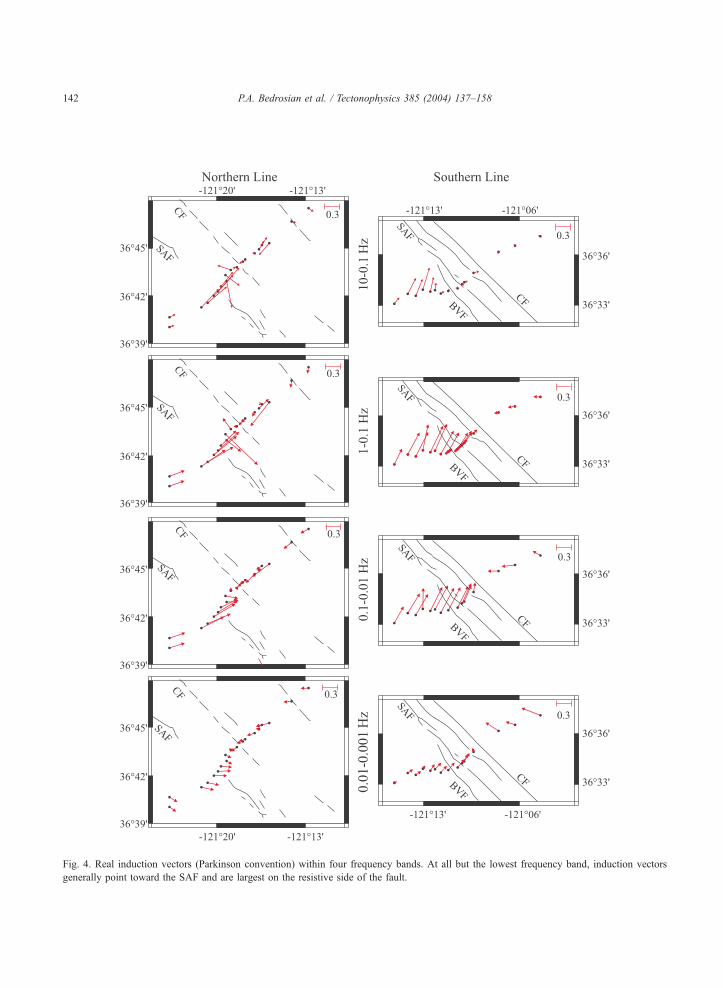
Fig. 4. Real induction vectors (Parkinson convention) within four frequency bands. At all but the lowest frequency band, induction vectors

generally point toward the SAF and are largest on the resistive side of the fault.



strike direction of N40jW to N45jW, in agreement

with the geologic strike of the SAF. Higher frequency

data for the southern profile deviate from this picture,

suggesting instead a north–south strike direction.

Despite this discrepancy, we chose to apply 2D

analysis and inversion to both profiles, rotating all

data to a fault-oriented coordinate system. This is

justified by the observation that above 1 Hz the

southern line, data are nearly identical regardless of

coordinate system. Furthermore, all inversions and

models to be discussed are based only upon the

sufficiently 2D data from 100 to 0.01 Hz. A discus-

sion of the low frequency data is beyond the scope of

this paper.

2.2. Magnetotelluric data

The data for both profiles are shown in pseudo-

section format in Figs. 5 and 6, respectively. The

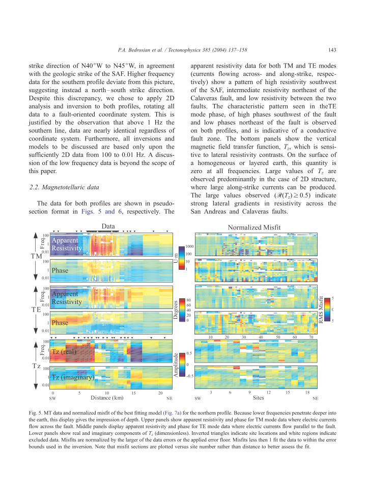
Fig. 5. MT data and normalized misfit of the best fitting model (Fig. 7a) for

the earth, this display gives the impression of depth. Upper panels show app

flow across the fault. Middle panels display apparent resistivity and phase

Lower panels show real and imaginary components of Tz (dimensionless).

excluded data. Misfits are normalized by the larger of the data errors or the

bounds used in the inversion. Note that misfit sections are plotted versus

apparent resistivity data for both TM and TE modes

(currents flowing across- and along-strike, respec-

tively) show a pattern of high resistivity southwest

of the SAF, intermediate resistivity northeast of the

Calaveras fault, and low resistivity between the two

faults. The characteristic pattern seen in theTE

mode phase, of high phases southwest of the fault

and low phases northeast of the fault is observed

on both profiles, and is indicative of a conductive

fault zone. The bottom panels show the vertical

magnetic field transfer function, Tz, which is sensi-

tive to lateral resistivity contrasts. On the surface of

a homogeneous or layered earth, this quantity is

zero at all frequencies. Large values of Tz are

observed predominantly in the case of 2D structure,

where large along-strike currents can be produced.

The large values observed (R(Tz)z 0.5) indicate

strong lateral gradients in resistivity across the

San Andreas and Calaveras faults.

the northern profile. Because lower frequencies penetrate deeper into

arent resistivity and phase for TM mode data where electric currents

for TE mode data where electric currents flow parallel to the fault.

Inverted triangles indicate site locations and white regions indicate

applied error floor. Misfits less then 1 fit the data to within the error

site number rather than distance to better assess the fit.

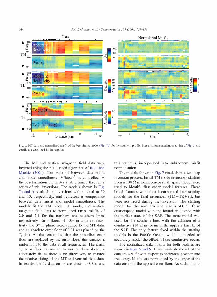
Fig. 6. MT data and normalized misfit of the best fitting model (Fig. 7b) for the southern profile. Presentation is analogous to that of Fig. 5 and

details are described in the caption.


The MT and vertical magnetic field data were

inverted using the regularized algorithm of Rodi and

Mackie (2001). The trade-off between data misfit

and model smoothness [j(logq)2] is controlled by

the regularization parameter s, determined through a

series of trial inversions. The models shown in Fig.

7a and b result from inversions with s equal to 50

and 10, respectively, and represent a compromise

between data misfit and model smoothness. The

models fit the TM mode, TE mode, and vertical

magnetic field data to normalized r.m.s. misfits of

2.0 and 2.1 for the northern and southern lines,

respectively. Error floors of 10% in apparent resis-

tivity and 3j in phase were applied to the MT data,

and an absolute error floor of 0.01 was placed on the

Tz data. All data errors less than the prescribed error

floor are replaced by the error floor; this ensures a

uniform fit to the data at all frequencies. The small

Tz error floor is needed to ensure these data are

adequately fit, as there is no direct way to enforce

the relative fitting of the MT and vertical field data.

In reality, the Tz data errors are closer to 0.05, and

this value is incorporated into subsequent misfit

normalization.

The models shown in Fig. 7 result from a two step

inversion process. Initial TM mode inversions starting

from a 100 V m homogeneous half space model were

used to identify first order model features. These

broad features were then incorporated into starting

models for the final inversions (TM+TE+ Tz), but

were not fixed during the inversion. The starting

model for the northern line was a 500/50 V m

quarterspace model with the boundary aligned with

the surface trace of the SAF. The same model was

used for the southern line, with the addition of a

conductive (10 V m) basin in the upper 2 km NE of

the SAF. The only feature fixed within the starting

models is the Pacific Ocean, which is needed to

accurately model the effects of the conductive ocean.

The normalized data misfits for both profiles are

shown in Figs. 5 and 6. These residuals show that the

data are well fit with respect to horizontal position and

frequency. Misfits are normalized by the larger of the

data errors or the applied error floor. As such, misfits

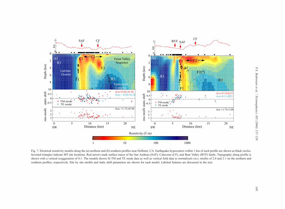
Fig. 7. Electrical resistivity models along the (a) northern and (b) southern profiles near Hollister, CA. Earthquake hypocenters within 1 km of each profile are shown as black circles.

Inverted triangles indicate MT site locations. Red arrows mark surface traces of the San Andreas (SAF), Calaveras (CF), and Bear Valley (BVF) faults. Topography along profile is

shown with a vertical exaggeration of 4:1. The models shown fit TM and TE mode data as well as vertical field data to normalized r.m.s. misfits of 2.0 and 2.1 on the northern and

southern profiles, respectively. Site by site misfits and static shift parameters are shown for each model. Labeled features are discussed in the text.

P.A.Bedrosia

net

al./Tecto

nophysics

385(2004)137–158

145


less then 1 fit the data to within the error bounds used

in the inversion. The average site misfit is 1.7F 0.6

on the northern line and 1.7F 1.1 on the southern

line. Note that the overall misfit and the average site

misfit are not directly comparable as they are calcu-

lated using different weightings.

Static shift parameters represent a frequency-inde-

pendent gain in the previously described tensor de-

composition. These parameters, one per mode at each

site, cannot be directly determined from the decom-

position, and were computed during the inversion. For

the TM mode, in which electric currents flow along

profile, continuous MT profiling (with a profile length

much larger than the near-surface inductive length)

imposes the constraint that the static shifts average to

zero along profile. This constraint, the result of charge

conservation, has been applied to both modes of the

MT data, although in the case of the TE mode data it

has no physical basis, and simply reduces the number

of degrees of freedom by one.

3. Discussion

3.1. Regional geolectric structure

A resistive body (R1) is imaged southwest of the

SAF on both profiles with resistivities greater than

1000 V m (Fig. 7). Constrained inversion studies

show that R1 need not be as resistive as imaged;

however, resistivities less than f 300 V m are in

compatible with the data. R1 is coincident with the

granodiorite of the Gabilan Range, part of the larger

Salinian block cut by the SAF through much of

central California (Ross, 1972). The uppermost few

hundred meters are less resistive and corresponds to a

surface-weathering zone. This uppermost layer is

thicker on the southern profile, perhaps due to alluvi-

um within Bickmore Canyon. R1 is uniform both

along strike and with increasing depth, particularly

along the northern profile. Coincident seismic studies

by Thurber et al. (1997) also imaged a homogeneous

velocity structure in this region.

Due to the high resistivity of R1, the natural EM

signals penetrate to greater depths in this region than

elsewhere on the profile, to depths of 50 km at the

lowest frequencies used (f 0.01 Hz). At a depth of

approximately 6 km, the resistivity of R1 decreases at

the southwest end of both profiles. While there is

adequate penetration, the conductor beneath the Gabi-

lan Range falls at the southwest edge of the profiles,

and is constrained by only one site on each profile.

Forward modeling studies indicate that this feature is

not strongly required by the data, which can be

equally fit by a conductor beyond the southwest end

of our profiles. It is thus possible that we are imaging

the relatively low resistivity of the coastal Franciscan

block (Jennings, 1977).

A decrease in resistivity was also noted by Phillips

and Kuckes (1983), who detected a conductive layer

at f 13-km depth beneath the Gabilan range close to

the northern profile. They hypothesized that the Gabi-

lans are locally underlain by serpentinized ocean

crust, a theory supported by seismic studies elsewhere

within the Salinian block (Howie et al., 1993; Hol-

brook et al., 1996). Walter and Mooney (1982),

however, argued instead that a granitic to gneissic

transition is responsible for an increase in seismic

velocity beneath the Gabilan range. It is interesting

that this feature does not extend as far northeast as the

SAF, but rather is separated from it by 6–8 km along

both profiles.

Northeast of the Calaveras fault, crustal resistivities

are moderate and increase with depth. The Franciscan

complex is presumed to form the basement in this

region, being locally overlain by the Cretaceous/

Tertiary Great Valley sequence (GVS). Additionally,

Quaternary sediments of the Hollister trough are

adjacent to and cut by the SAF. The GVS is exposed

in outcrop along the length of the Diablo Range and

has a thickness of 6–8 km (Dickinson, 2002; Fielding

et al., 1984). A strong resistivity gradient at 7–8-km

depth to the northeast of the Calaveras fault may

represent the boundary between the GVS and the

underlying Franciscan complex.

An asymmetric region of enhanced electrical con-

ductivity (C2) is found between the SAF and Cala-

veras fault. The geometry of this zone is similar on

both profiles; its deepest part (C1) is located beneath

the SAF and stops abruptly to the southwest. Such a

sharp lateral resistivity variation is not imaged to the

northeast. Coincident, asymmetric low-velocity zones

have been imaged by Thurber et al. (1997) and Feng

and McEvilly (1983) along the northern and southern

profiles, respectively. The high-conductivity zone, C2,

additionally appears to be divided into discrete pock-


ets divided by northeast dipping zones of higher

resistivity. The resistivity of these zones drops to 1

V m, while the average is closer to 5 V m. A detailed

discussion of the nature of this region is presented in

the following sections.

To first order, the electrical structure observed is

quite similar along the northern and southern profiles.

Significant differences are, however, apparent be-

tween the two profiles. Crossing the southern profile,

the Bear Valley fault (BVF) is located southwest of

the San Andreas fault and runs parallel to it for f 15

km along strike. This fault shows no evidence of

Holocene movement and even its very nature has been

called into question by Dibblee (1966) who interprets

it as an unconformity of nontectonic origin. Electri-

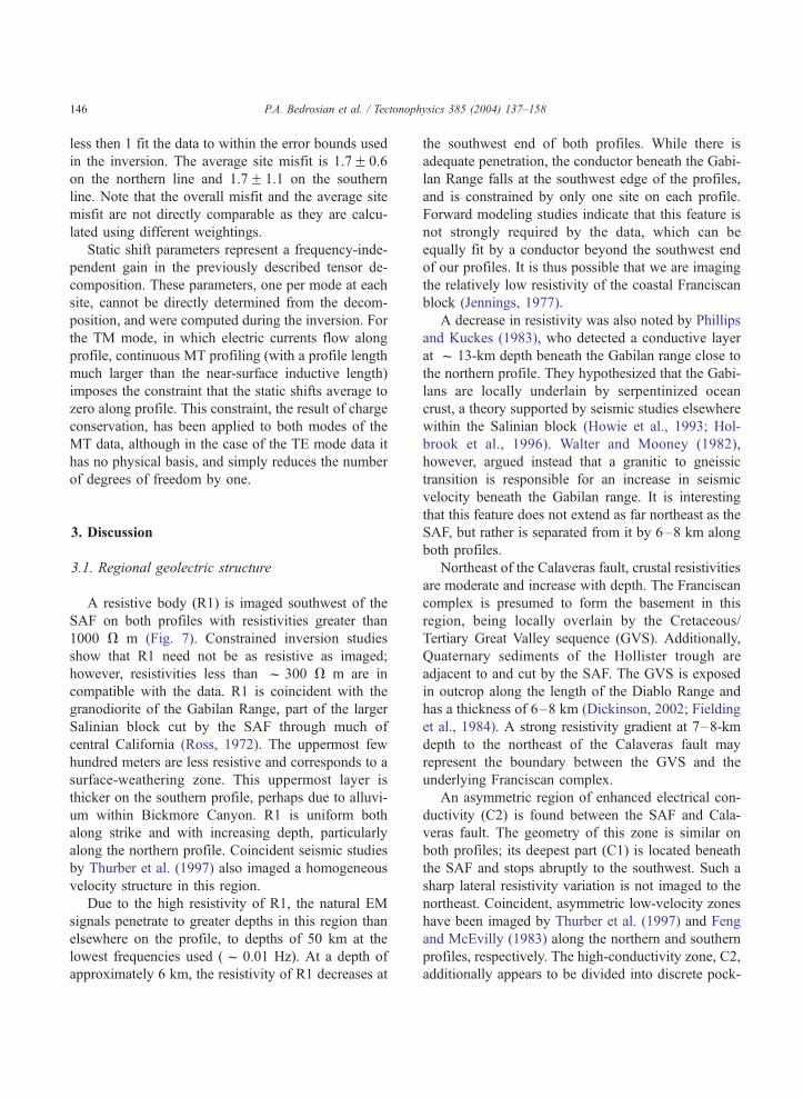
Fig. 8. Modified southern line resistivity models and associated misfit. Con

range of depths. Subsequent inversion of these models, with structure fixed

terminated at 2.5 km, (b) conductor terminated at 1 km, (c) conductor com

average is taken over sites within 1 km of the conductor and is normalized t

surface trace.

cally, the BVF is imaged as a thin (f 500 m wide)

zone of enhanced conductivity extending to 2–3-km

depth (Fig. 7), a signature suggestive of a tectonic

origin for the BVF. The surface trace of the Bear

Valley fault lies near the northeast edge of this zone.

A constrained inversion study was undertaken to

determine if this conductor is a required feature of the

model, or whether the data can be equally fit with a

shallower conductor. The conductor imaged in Fig. 7b

was truncated at a range of depths (0, 0.5, 1, 2.5 km

depth) and the inversion restarted with the constraint

that the resistivity model remain fixed in the region of

modification. Visual inspection of a subset of the

resulting models (Fig. 8) reveals that the misfit of

the constrained inversion models differ minimally

ductive zone adjacent to the Bear Valley fault has been truncated at a

below the truncation, gave rise to the above models. (a) Conductor

pletely removed, (d) average site misfit vs. depth of conductor. The

o that of the best fit model (Fig. 7b). Arrow denotes location of BVF


from the best fit model unless the conductor is

terminated at 0.5-km depth or completely removed.

In these two cases, increased conductivity is mapped

onto neighboring structure, giving rise to conductive

wings extending to 2-km depth. Fig. 8d shows the

average site misfit (normalized to that of the best fit

model) for sites located within 1 km of the conductor.

Note the significant rise in site misfit when the

conductor is truncated at depths shallower than 1

km. These studies suggest that the conductive halo

extending to 5 km beneath the BVF is not a required

feature of the model. However, the conductor adjacent

to the BVF is a robust feature, and is required to

extend to at least 1 km.

Below the imaged conductor, moderate resistivities

appear to separate the Gabilan granites (R1) from a

resistive sliver to the northeast. Further modeling

found that the replacement of this gap with a resistive

bridge is inconsistent with the data. This suggests that

a fault slice may be bound between the Bear Valley

and San Andreas faults; however, without knowing

the depth extent of the BVF, such an assertion is

speculative. To the east, the high-conductivity region,

C2, extends at least 5 km east of the Calaveras fault,

in contrast to the northern profile, where it terminates

more abruptly at the Calaveras fault. Furthermore, on

the southern profile, C2 appears relatively homoge-

neous. This, however, most probably reflects the

sparsity of sites along this part of the profile rather

than a lack of structural detail.

3.2. Fault-zone geometry

The resistivity models for both profiles suggest that

zones of enhanced conductivity are bounded by the

San Andreas and Calaveras faults; however, MT is not

always able to delineate the edges of structures. In

order to further evaluate the models, other geological

and geophysical data were analyzed. This included (1)

the regional seismicity, (2) seismic tomography, and

(3) constrained MT inversion studies.

Seismicity along the SAF system is generally

shallow; few regions exhibit seismicity below 10–

15 km, the depth of the brittle–ductile transition

(Brace and Byerlee, 1970). The resistivity models in

Fig. 7 are overlain with the locations of earthquake

hypocenters within 1 km of each profile (Mz 1.0).

Earthquake hypocenters have been relocated using the

method of Waldhauser and Ellsworth (2000) applied

to P-wave picks from the NCSN catalog (Ellsworth et

al., 2000). Given the quality of the earthquake catalog,

this method can determine relative hypocenter loca-

tions to within 25–50 m; however, the absolute

location errors may be significantly larger (Bill Ells-

worth, pers. comm.; Waldhauser and Ellsworth,

2002).

Seismicity on the SAF defines a near-vertical plane

on both profiles, extending from 3 to 7 km depth on

the northern line and 2–9 km depth on the southern

line. On the northern line, seismicity lies f 1.5 km

southwest of the surface trace, a result also observed

by Thurber et al. (1997) in determining hypocenters

from a 2D velocity model. Further to the northeast, a

northeast dipping (70j) plane of seismicity is evident

on the northern line. As this seismicity is deeper (6–

11 km) and not well localized, it is unclear to what

mapped fault it projects. To the northwest, the seis-

micity appears associated with the Calaveras fault;

however, it is located several kilometers northeast of

the Calaveras surface trace. A linear projection of this

seismicity to the surface falls within f 500 m of the

surface trace; however, this infers a significant dip to

this predominantly strike-slip fault. Furthermore,

earthquake focal mechanisms in the immediate region

are in agreement with dextral strike-slip on vertical

fault planes (Ellsworth, 1975). The solution may lie in

the high spatial variability of seismicity along the

southern Calaveras fault, with some areas devoid of

seismicity, while others show events clustered along a

vertical plane, and still others areas exhibit a promi-

nently dipping fault plane. In the case at hand, the

dipping fault can be traced for only 3–4 km along-

strike, and is thus most probably a local feature rather

than a characteristic of the Calaveras fault.

The seismicity associated with the San Andreas

fault locates at the southwest edge of conductive zone

C1, hereafter referred to as the fault-zone conductor

(FZC). This geometric relationship is seen on both

profiles at Hollister (Bedrosian et al., 2002) as well as

on a series of profiles at Parkfield (Unsworth et al.,

1997), At Hollister, however, the FZC extends to

greater depth than at Parkfield. It is also of note that

little or no seismicity is seen within zones C1 and C2

on either profile. Finally, there is not a clear electrical

signature of the Calaveras fault below 4 km. If the

Calaveras fault is steeply dipping, as the seismicity


suggests, then there is no resistivity change associated

with the fault as it cuts through the Franciscan (R2). If

on the other hand, the Calaveras fault is vertical (and

hence locally a seismic), then the moderate northeast-

ward increase in resistivity at depth may represent

different structural units juxtaposed across the fault.

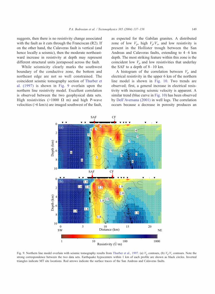
While seismicity clearly marks the southwest

boundary of the conductive zone, the bottom and

northeast edge are not so well constrained. The

coincident seismic tomography section of Thurber et

al. (1997) is shown in Fig. 9 overlain upon the

northern line resistivity model. Excellent correlation

is observed between the two geophysical data sets.

High resistivities (>1000 V m) and high P-wave

velocities (>6 km/s) are imaged southwest of the fault,

Fig. 9. Northern line model overlain with seismic tomography results from

strong correspondence between the two data sets. Earthquake hypocenter

triangles indicate MT site locations. Red arrows indicate the surface trace

as expected for the Gabilan granites. A distributed

zone of low Vp, high Vp/Vs, and low resistivity is

present in the Hollister trough between the San

Andreas and Calaveras faults, extending to 4–6 km

depth. The most striking feature within this zone is the

coincident low Vp and low resistivities that underlay

the SAF to a depth of 8–10 km.

A histogram of the correlation between Vp and

electrical resistivity in the upper 6 km of the northern

line model is shown in Fig. 10. Two trends are

observed; first, a general increase in electrical resis-

tivity with increasing seismic velocity is apparent. A

similar trend (blue curve in Fig. 10) has been observed

by Dell’Aversana (2001) in well logs. The correlation

occurs because a decrease in porosity produces an

Thurber et al., 1997. (a) Vp contours, (b) Vp/Vs contours. Note the

s within 1 km of each profile are shown as black circles. Inverted

s of the San Andreas and Calaveras faults.

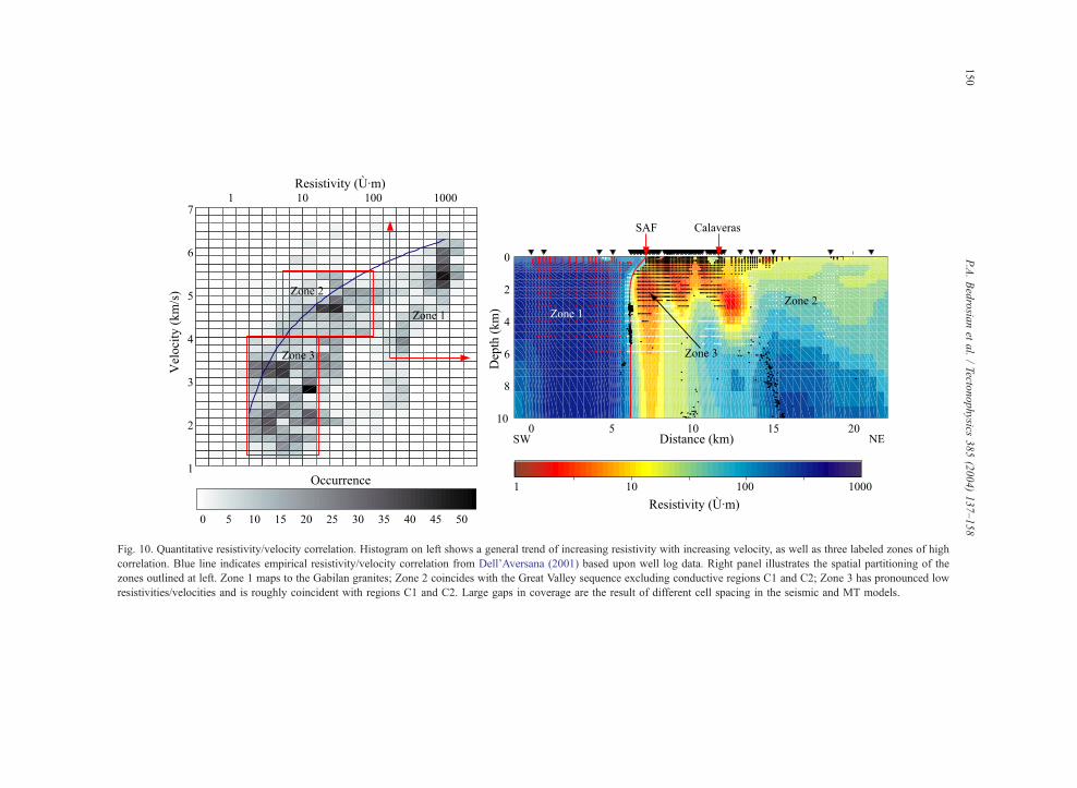
Fig. 10. Quantitative resistivity/velocity correlation. Histogram on left shows a general trend of increasing resistivity with increasing velocity, as well as three labeled zones of high

correlation. Blue line indicates empirical resistivity/velocity correlation from Dell’Aversana (2001) based upon well log data. Right panel illustrates the spatial partitioning of the

zones outlined at left. Zone 1 maps to the Gabilan granites; Zone 2 coincides with the Great Valley sequence excluding conductive regions C1 and C2; Zone 3 has pronounced low

resistivities/velocities and is roughly coincident with regions C1 and C2. Large gaps in coverage are the result of different cell spacing in the seismic and MT models.

P.A.Bedrosia

net

al./Tecto

nophysics

385(2004)137–158

150


increase in both seismic velocity and resistivity. Sec-

ond, localized zones of high correlation are observed.

These are clusters showing common resistivities and

velocities, and are not to be confused with previously

described features (C1, C2, R1, R2) based solely on

the MT models. Due to the coarse grid of the

histogram (limited by the size of the seismic model

grid), only three zones have been chosen. The right

panel of Fig. 10 shows the spatial regions from which

these zones derive. The region of high resistivity/

velocity (zone 1) corresponds exclusively to the

Gabilan granites. Zones 2 and 3 are defined by

significantly lower resistivity/velocity and are located

to the northeast of the SAF, overlaying large portions

of the region between the SAF and Calaveras faults,

as well as the upper 4 km northeast of the Calaveras.

The localization of these zones both spatially and

in resistivity/velocity space suggest they delineate

characteristic subsets of the data with (relatively)

uniform material properties. For tectonic investiga-

tions, it is the boundaries between these zones that are

of most interest. Zones 1 and 2 represent different

geologic units (the Gabilan granites and the Great

Valley sequence, respectively), while the boundary

between zones 2 and 3 likely represents a hydrologic

boundary between saturated and dry regions of the

GVS. Hints of this undulating boundary are evident in

the individual data sets; however, it is more clearly

defined in this combined view. Additionally, the SAF

is imaged as a narrow strip of low resistivity/velocity

between zones 1 and 2, which also coincides with the

plane of seismicity. Therefore, the combination of

electrical and seismic data, along with seismicity

patterns, are able to constrain the location of the San

Andreas fault at depth to a narrow plane at the

southwest edge of the imaged FZC.

Finally, the southwest boundary of zone 3 smooth-

ly connects the surface trace of the SAF to the

seismically defined SAF at depth. This southwest-

dipping boundary is interpreted as the fault plane of

the SAF in the upper 2 km. Gravity studies by Pavoni

(1973) in the vicinity of the northern profile favor a

steeply dipping (67–70j) SAF in the upper 5 km,

with a vertical fault below. The MT data are incon-

sistent with a vertical SAF, and suggest a dip of 55j inthe upper 2 km; however, a slightly steeper dip may

be permissible. Assuming the density of zone 3 is less

than zone 1 (a reasonable assumption given the much

lower seismic velocity of zone 3), both the MT and

gravity models emplace lower density material f 2

km southwest of the surface trace of the SAF. Given

the appropriate density contrast across the fault, the

geometry we image may be able to reproduce the

measured gravity anomaly. In contrast, the MT model

for the southern profile suggests a near vertical fault

plane to within 1 km of the surface, above which no

clear resistivity contrast is imaged. Seismic (Feng and

McEvilly, 1983) and gravity (Wang et al., 1986)

models of the Bear Valley profile also show a vertical

SAF. Thus, the upper-crustal geometry of the San

Andreas fault appears to vary significantly on a length

scale of tens of kilometers.

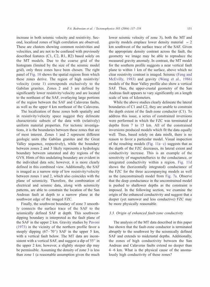
While the above studies clearly delineate the lateral

boundaries of C1 and C2, they are unable to constrain

the depth extent of the fault-zone conductor (C1). To

address this issue, a series of constrained inversions

were performed in which the FZC was terminated at

depths from 7 to 15 km. All of the constrained

inversions produced models which fit the data equally

well. Thus, based solely on data misfit, there is no

reason to favor a particular model. Visual inspection

of the resulting models (Fig. 11a–c) suggests that as

the depth of the FZC decreases, its lateral extent and

conductivity increase. This is an example of the

sensitivity of magnetotellurics to the conductance, or

integrated conductivity within a region. Fig. 11d

shows the (horizontally integrated) conductance of

the FZC for the three accompanying models as well

as the (unconstrained) model from Fig. 7a. Observe

that the deep conductance in the unconstrained model

is pushed to shallower depths as the constraint is

imposed. In the following section, we examine the

origin of the enhanced conductivity and suggest that a

deeper (yet narrower and less conductive) FZC may

be more physically reasonable.

3.3. Origin of enhanced fault-zone conductivity

The analysis of the MT data described in this paper

has shown that the fault-zone conductor is terminated

abruptly to the southwest by the seismically defined

SAF and extends to midcrustal depths. Additionally,

the zones of high conductivity between the San

Andreas and Calaveras faults extend no deeper than

4–6 km. What is the physical cause of the anoma-

lously high conductivity of these zones?

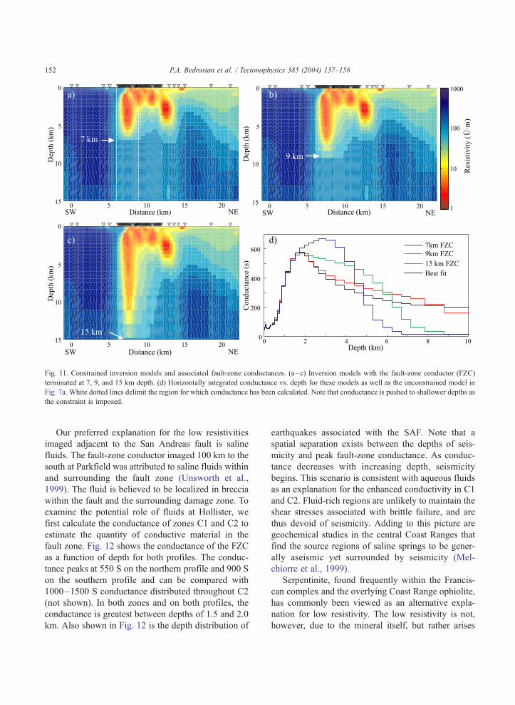
Fig. 11. Constrained inversion models and associated fault-zone conductances. (a–c) Inversion models with the fault-zone conductor (FZC)

terminated at 7, 9, and 15 km depth. (d) Horizontally integrated conductance vs. depth for these models as well as the unconstrained model in

Fig. 7a. White dotted lines delimit the region for which conductance has been calculated. Note that conductance is pushed to shallower depths as

the constraint is imposed.


Our preferred explanation for the low resistivities

imaged adjacent to the San Andreas fault is saline

fluids. The fault-zone conductor imaged 100 km to the

south at Parkfield was attributed to saline fluids within

and surrounding the fault zone (Unsworth et al.,

1999). The fluid is believed to be localized in breccia

within the fault and the surrounding damage zone. To

examine the potential role of fluids at Hollister, we

first calculate the conductance of zones C1 and C2 to

estimate the quantity of conductive material in the

fault zone. Fig. 12 shows the conductance of the FZC

as a function of depth for both profiles. The conduc-

tance peaks at 550 S on the northern profile and 900 S

on the southern profile and can be compared with

1000–1500 S conductance distributed throughout C2

(not shown). In both zones and on both profiles, the

conductance is greatest between depths of 1.5 and 2.0

km. Also shown in Fig. 12 is the depth distribution of

earthquakes associated with the SAF. Note that a

spatial separation exists between the depths of seis-

micity and peak fault-zone conductance. As conduc-

tance decreases with increasing depth, seismicity

begins. This scenario is consistent with aqueous fluids

as an explanation for the enhanced conductivity in C1

and C2. Fluid-rich regions are unlikely to maintain the

shear stresses associated with brittle failure, and are

thus devoid of seismicity. Adding to this picture are

geochemical studies in the central Coast Ranges that

find the source regions of saline springs to be gener-

ally aseismic yet surrounded by seismicity (Mel-

chiorre et al., 1999).

Serpentinite, found frequently within the Francis-

can complex and the overlying Coast Range ophiolite,

has commonly been viewed as an alternative expla-

nation for low resistivity. The low resistivity is not,

however, due to the mineral itself, but rather arises

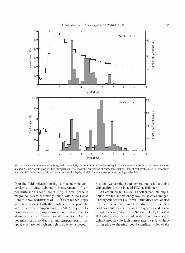
Fig. 12. Conductance (horizontally integrated conductivity) of the FZC as a function of depth. Conductance is observed to be largest between

0.5 and 2.5 km on both profiles. The histograms in gray show the distribution of earthquakes within 1 km of each profile (M>1.0) associated

with the SAF. Note the spatial separation between the depths of high fault-zone conductance and high seismicity.


from the fluids released during its metamorphic con-

version to olivine. Laboratory measurements of ser-

pentinite-rich rocks containing a few percent

magnetite, as are commonly found within the Coast

Ranges, show resistivities of 104 V m or higher (Popp

and Kern, 1993). Both the existence of serpentinite

and the elevated temperatures (f 500j) required to

bring about its decomposition are needed in order to

attain the low resistivities often attributed to it. As it is

not intrinsically conductive, and temperatures in the

upper crust are not high enough to activate its decom-

position, we conclude that serpentinite is not a viable

explanation for the imaged FZC at Hollister.

An entrained fault slice is another possible expla-

nation for the anomalously low resistivities imaged.

Throughout central California, fault slices are located

between active and inactive strands of the San

Andreas fault system. Slivers of igneous and meta-

morphic rocks (parts of the Salinian block, the Gold

Hill gabbros) within the SAF system tend, however, to

exhibit moderate to high resistivities. Pervasive frac-

turing (due to shearing) could significantly lower the


bulk resistivity; however, such fracturing would also

weaken the sliver, making it unlikely to survive intact

after significant transport along the fault. In short,

given the degree of fracturing necessary to explain the

low resistivity, any sliver would likely be ground up

by the fault during transport.

Having discussed several alternative sources of

high conductivity, were turn to aqueous fluids. How

much fluid is needed to account for the observed

resistivity? A porosity of 9–30%, saturated with

aqueous fluids was necessary to explain the conduc-

tivity anomaly observed in the San Andreas fault at

Parkfield (Unsworth et al., 1999). To relate electrical

resistivity to porosity an estimate of the fluid salinity

must be established. Salinities of 17 mg/l were mea-

sured in the Stone Canyon well, a 600-m-deep arte-

sian well located within the Gabilan granite (Fig. 1)

midway between the two profiles and 1 km from the

SAF (Stierman and Williams, 1984; J. Thordsen, pers.

comm.). Archie’s law can be used torelate the fluid

resistivity (a function of salinity and temperature) and

porosity of a fluid saturated rock to its bulk resistivity.

Combining the average resistivity (5 V m) of the FZC

at 1.5-km depth (the depth of peak conductance) with

the salinity from the Stone Canyon well, a porosity

range of 15–35% is obtained. The limits reflect the

geometry of the pores; upper and lower limits corre-

spond to spherical pores and cracks, respectively, the

latter being a reasonable assumption surrounding an

active fault zone. It should be noted that these

estimates place an upper bound on porosity, as the

presence of clay minerals within the fault zone will

further decrease electrical resistivity. It is unclear,

however, how to quantitatively address either the

amount and distribution of clay in the fault zone or

its effect on resistivity. That the stated porosities

represent an upper bound is additionally based upon

fluid salinities. Salinities are generally higher on the

northeast side of the fault, as at the Varian well near

Parkfield (Jongmans and Malin, 1995), and increasing

fluid salinity decreases the required porosity. Unfor-

tunately, salinity measurements from the northeast

side of the fault are not available within the survey

region.

The porosities estimated at shallow depths are in

agreement with independent porosity estimates. Grav-

ity studies in Bear Valley by Wang et al. (1986)

suggest a low-density wedge centered on the San

Andreas fault zone extending to the base of the

seismogenic zone. The authors calculate a lower

porosity bound of 12% for this region; however, the

modeling assumes a constant density (and hence

porosity) from the surface to f 15-km depth. In

reality, a decrease in porosity is expected with in-

creasing depth as confining pressure increases. At

depths approaching the brittle–ductile transition, the

resistivity of the fault zone increases to around 10 V

m. The effect of increasing pressure and temperature,

however, cause fluid resistivity, and in turn bulk

resistivity, to decrease. Taken together, the MT data

suggest porosities of 2–15% at 10 km depth beneath

the SAF. We again favor the lower end of this range

for the reasons cited above. The presence of a few

percent porosity at such depths may result from small

and recoverable volumetric strain due to shearing.

At this point, we revisit the question of the depth

extent of the fault-zone conductor. As discussed

before, limiting the depth extent of the FZC results

in a broadening and intensification of the remaining

structure. This results in higher porosities being re-

quired to explain the low resistivity. For example, if

the FZC is terminated at 7 km depth as in Fig. 11a,

porosities of up to 50% at 1.5 km and 15% at 5 km

depth are needed. As these values appear unrealistic,

we favor a model with a narrower and deeper FZC

(Fig. 11c) which requires more moderate porosities to

account for the decreased resistivity within the fault

zone.

The source of fault-zone fluids remains uncertain.

Irwin and Barnes (1975) suggest they may emanate

from metamorphic reactions within the Franciscan

complex, transported laterally into the fault zone.

Geochemical studies of fault-zone materials by Pili et

al. (1998) support this conclusion and suggest that

during deformation the fault zone is infiltrated by

mixed H2O–CO2 fluids of metamorphic or deep

crustal origin. In contrast, the geochemical signature

of spring and well fluids along the SAF suggest a

meteoric fluid origin, with a maximum circulation

depth of 6 km (Kharaka et al., 1999). This is compa-

rable to the depth at which estimated porosities fall

below 10%. Finally, a high flux of mantle-derived CO2

is inferred by Kennedy et al. (1997) based on helium

isotopic ratios in springs and seeps along the SAF.

To interpret the electrical images of the San

Andreas, it is essential to compare the geophysical


models with geological observations of exhumed fault

zones (Chester and Logan, 1986; Chester et al., 1993).

The highest conductivities are observed in the upper

2–3 km of the San Andreas fault, both at Parkfield

and Hollister. As described above, relatively high

porosities are required to account for the observed

low resistivity. Thus, the shallow part of the fault zone

is probably a zone of fault breccias (Anderson et al.,

1983). This is surrounded by the damage zone, a

region of pervasive fracturing (Caine et al., 1996).

Saline fluids present in the fault will readily fill voids

in the breccia and fractures within the damage zone,

resulting in the observed low resistivity. As depth

increases, geological studies have shown that catacla-

sites and mylonites are formed in the fault zone at

higher ambient pressure and temperature. These are

presumably present in the creeping San Andreas fault

at Hollister in the 4–10-km depth range. The resis-

tivity models derived from the MT data show that

significant porosity is present in this depth range

where the fault may be expressed as a distributed

zone of shearing.

The abrupt southwest boundary of C1 and the

sharp northeast dipping boundaries within C2 (cut-

ting stratigraphic horizons) suggest that fluid distri-

bution is tectonically controlled. Other studies have

indicated that faults can act both as conduits for

along-strike fluid flow and as barriers for across-

Fig. 13. Geophysical model of the San Andreas fault-zone along the northe

faults are denoted. White circles indicate seismicity within 1 km of the pro

15–35%. The most extensive zone is located adjacent to the SAF and is at

the fault. High conductivity at greater depths is attributed to fluid-filled, f

strike flow (Ritter et al., 2003; Caine et al., 1996).

We conclude that the dipping boundaries within C2

represent fault seals separating pockets of fluid-

saturated rock. Our 2D profiles cannot address

whether these faults additionally act as conduits,

but 3D tomographic modeling images a continuous

low Vp zone extending for at least 10 km along

strike.

4. Conclusions

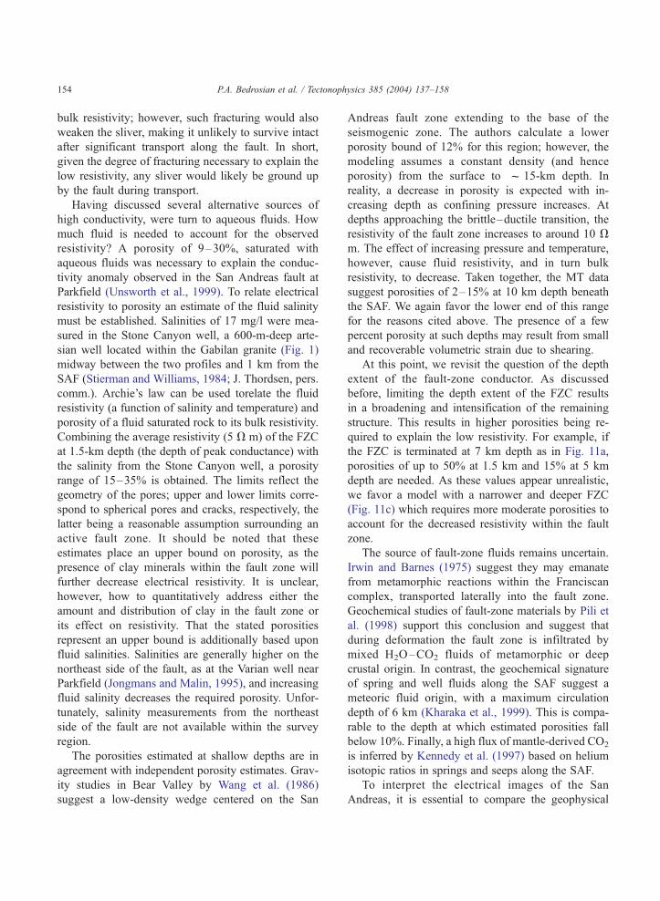
Based upon the MT and seismic studies at Hollis-

ter, an integrated geophysical model is proposed (Fig.

13) for the northern profile. Within the creeping

segment south of Hollister, CA, the San Andreas fault

is characterized by a zone of low resistivity extending

from the San Andreas fault to the Calaveras fault. This

zone of low resistivity is imaged on both profiles and

in the upper 2–3 km is attributed to fluid filled voids

and fractures within the brecciated and damaged zone

of the fault (Caine et al., 1996; Anderson et al., 1983).

These conductivity values can be accounted for by a

porosity of 15–35% of aqueous fluids. These values

represent an upper bound due to the possible effect of

clays within the fault zone. The conductance of the

fault zone decreases with depth, but the conductivity

remains significantly higher than expected for dry

rn profile. Surface traces of San Andreas (SAF) and Calaveras (CF)

file. Dashed zones denote fluid-saturated regions with porosities of

tributed to fluid filled voids and fractures within the damage zone of

ault-aligned cracks within a broad zone of shearing.


midcrustal rocks. This is possibly due to 2–15%

fluids present in fault aligned cracks.

The combination of seismic and magnetotelluric

data has determined that the SAF is vertical below 2

km depth, and is located on the southwest edge of the

imaged fault-zone conductor. The low resistivity be-

tween the San Andreas and Calaveras faults is dis-

tributed in localized zones interpreted as fluid pockets

separated from one another by northeast dipping,

impermeable fault seals. In combination with previous

MT studies at Carrizo Plain and Parkfield, these

results suggest a relationship between seismicity and

fluid supply from the Franciscan complex to the fault

zone. At Parkfield and Hollister where the fault

creeps, the breccia and damage zones are saturated

with fluids (presumably derived from the Franciscan

complex). In contrast, at Carrizo Plain the east wall of

the San Andreas fault is resistive, crystalline rock

devoid of fluid pathways. The fault here is locked and

fractures in the damaged zone are relatively dry.

How is the fluid regime of the San Andreas fault

related to it’s seismic behavior? In one scenario, fluids

could be controlling the seismic behavior. It should be

noted that the FZC, and thus the inferred fluids, is best

resolved at relatively shallow depths, well above the

source region of major earthquakes. However, a fluid

saturated shallow fault zone suggests fluids could be

present at greater depth. These fluids, if isolated and

over pressured, may control the mechanics of faulting

as envisioned by Byerlee (1993) and Sleep and

Blanpied (1992). In this scenario, significant changes

in the electrical structure of the San Andreas fault may

be observable immediately following a moderate to

large earthquake in central California. Unfortunately,

MT can only image the distribution of fluids within

and surrounding the fault zone; in situ studies alone

are able to determine whether such fluids are at or

above hydrostatic pressure. In an alternate scenario,

fluids surrounding the SAF may simply be a conse-

quence of a creeping fault rather than a controlling

factor. A segment of the fault that is creeping is likely

to develop and maintain an interconnected network of

fractures. When saline groundwater fills these cracks,

the resistivity decreases. Further understanding of

these phenomena will require additional geophysical

data. This includes 3D studies of the San Andreas and

other major strike-slip faults, and studies of the same

location throughout the seismic cycle.

Acknowledgements

The MT component of this study was supported by

DOE Grant DEEG03-97ER-14781, NSF grant

EAR9614411, and USGS grants 1434-HQ-97-GR-

03157and 1434-HQ-97-GR-03152. The seismic com-

ponent was supported by NSF grant EAR-9317030

with additional support from the Deep Continental

Studies program of the USGS. The seismic instru-

ments used were provided by the PASSCAL facility

of IRIS. MT instruments were provided by the

EMSOC consortium. Parkfield MT data were provid-

ed courtesy of the Berkeley Seismological Laboratory.

Earthquake hypocenters are from the Northern

California Seismic Network. Both of these data sets

are archived and distributed by the Northern Cal-

ifornia Earthquake Data Center. We wish to thank the

area landowners who graciously allowed access to

their property, and to T. Burdette for assistance with

permitting. Finally, this study would not have been

possible without much enthusiastic field help (Sierra

Boyd, Jerry Casson, Shawn Cokus, Nick Hayman,

Michelle Koppes, Shenghui Li, Gillian Sharer, and

John Sylwester). We thank Stephen Park and Mark

Zoback for their reviews and Associate Editor Tuncay

Taymaz for suggestions, both of which greatly

improved this paper.

References

Allen, C., 1968. The tectonic environments of seismically active

and inactive areas along the San Andreas fault system. In: Dick-

inson, W.R., Grantz, A. (Eds.), Proceedings of Conference on

Geologic Problems of the San Andreas Fault System. Stanford

University Publications, pp. 70–82.

Anderson, J.L., Osbourne, R.H., Palmer, D.F., 1983. Cataclastic

rocks of the San Gabriel fault: an expression of deformation

at deeper levels in the San Andreas fault zone. Tectonophysics

98, 209–251.

Bedrosian, P.A., Unsworth, M.J., Egbert, G., 2002. Magnetotelluric

imaging of the creeping segment of the San Andreas fault near

Hollister. Geophys. Res. Lett. 29, 1–4.

Boyd, O.S., Egbert, G.D., Eisel, M., Morrison, H.F., 1997. A pre-

liminary analysis of the Parkfield EM field monitoring network.

EOS Trans. AGU 78, 489.

Brace, W.F., Byerlee, J.D., 1970. California earthquakes: why only

shallow focus? Science 168, 1573–1575.

Byerlee, J., 1993. Model for episodic flow of high-pressure water in

fault zones before earthquakes. Geology 21, 303–306.


Caine, J.S., Evans, J.P., Forster, C.B., 1996. Fault zone architecture

and permeability structure. Geology 24, 1025–1028.

Chester, F.M., Logan, J.M., 1986. Implications for mechanical

properties of brittle faults from observations of the Punchbowl

fault zone, California. Pure Appl. Geophys. 124, 79–106.

Chester, F.M., Evans, J.P., Biegel, R.L., 1993. Internal structure and

weakening mechanisms of the San Andreas fault. J. Geophys.

Res. 98, 771–786.

Dell’Aversana, P., 2001. Integration of seismic, MT, and gravity

data in a thrust belt interpretation. First Break 19, 335–341.

Dibblee Jr., T.W., 1966. Evidence for cumulative offset on the San

Andreas fault in central and northern California. Bull.-Calif.,

Div. Mines Geol. 190, 375–384.

Dickinson, W.R., 2002. Reappraisal of hypothetical Franciscan

thrust wedging at Coalinga: implications for tectonic relations

along the Great Valley flank of the California Coast Ranges.

Tectonics 29 (doi: 10.1029/2001TC001315).

Egbert, G.D., 1997. Robust multiple station magnetotelluric data

processing. Geophys. J. Int. 130, 475–496.

Egbert, G.D., Booker, J.R., 1986. Robust estimation of geomagnet-

ic transfer functions. Geophys. J. R. Astron. Soc. 87, 173–194.

Egbert, G.D., Eisel, M., Boyd, O.S., Morrison, H.F., 2000. DC

trains and PC3s: source effects in mid-latitude geomagnetic

transfer functions. Geophys. Res. Lett. 27, 25–28.

Ellsworth, W.L., 1975. Bear Valley, California, earthquake se-

quence of February–March 1972. Bull. Seismol. Soc. Am.

65, 483–506.

Ellsworth, W.L., Beroza, G.C., Julian, B.R., Klein, F., Michael,

A.J., Oppenheimer, D.H., Prejean, S.G., Richards-Dinger,

K., Ross, S.L., Schaff, D.P., Waldhauser, F., 2000. Seismic-

ity of the San Andreas Fault system in central California: appli-

cation of the double-difference location algorithm, on a regional

scale. EOS, Trans. AGU 81 (48), 919.

Feng, R., McEvilly, T.V., 1983. Interpretation of seismic reflection

profiling data for the structure of the San Andreas fault zone.

Bull. Seismol. Soc. Am. 73, 1701–1720.

Fielding, E., Barazangi,M., Brown, L., Oliver, J., Kaufman, S., 1984.

COCORP seismic profiles near Coalinga, California: subsurface

structure of the western Great Valley. Geology 12, 268–273.

Gamble, T.D., Goubau, W.M., Clarke, J., 1979. Magnetotellurics

with a remote reference. Geophysics 44, 53–68.

Groom, R.W., Bailey, R.C., 1989. Decomposition of magnetotellu-

ric impedance tensors in the presence of local three-dimensional

galvanic distortion. J. Geophys. Res. 94, 1913–1925.

Holbrook, W.S., Brocher, T.M., ten Brink, U.S., Hole, J.A., 1996.

Crustal structure of a transform plate boundary: San Francisco

bay and the California continental margin. J. Geophys. Res. 101,

22311–22334.

Howie, J.M., Miller, K.C., Savage, W.U., 1993. Integrated crustal

structure across the south central California margin: Santa Lucia

escarpment to the San Andreas fault. J. Geophys. Res. 98,

8173–8196.

Irwin, W.P., Barnes, I., 1975. Effect of geologic structure and meta-

morphic fluids on seismic behavior of the San Andreas fault

system in Central and Northern California. Geology 3, 713–716.

Jennings, C.W., 1977. Geologic map of California, California Geo-

logical Survey, scale 1:750,000.

Jongmans, P.A., Malin, P.E., 1995. Microearthquake S-wave obser-

vations from 0 to 1 km in the Varian well at Parkfield, Califor-

nia. Bull. Seismol. Soc. Am. 85, 1805–1821.

Kennedy, B.M., Kharaka, Y.K., Evans, W.C., Ellwood, A.,

DePaolo, D.J., Thordsen, J., Ambats, G., Mariner, R.H., 1997.

Mantle fluids in the San Andreas fault system, California. Sci-

ence 278, 1278–1281.

Kharaka, Y.K., Thordsen, J.J., Evans, W.C., Kennedy, B.M., 1999.

Geochemistry and hydromechanical interactions of fluids asso-

ciated with the San Andreas fault system, California. In: Hane-

berg, W.C., Mosely, P.S., Moore, J.C., Goodwin, L.B. (Eds.),

Faults and Subsurface Fluid Flow in the Shallow Crust. Geo-

physical Monograph, vol. 113. American Geophysical Union,

Washington, pp. 129–148.

Mackie, R.L., Livelybrooks, D.W., Madden, T.R., Larsen, J.C.,

1997. A magnetotelluric investigation of the San Andreas

fault at Carrizo Plain, California. Geophys. Res. Lett. 24,

1847–1850.

McNeice, G.W., Jones, A.G., 2001. Multisite, multifrequency ten-

sor decomposition of magnetotelluric data. Geophysics 66,

158–173.

Melchiorre, E.B., Criss, R.E., Davisson, M.L., 1999. Relationship

between seismicity and subsurface fluids, central Coast Ranges,

California. J. Geophys. Res. 104, 921–939.

Mount, V.S., Suppe, J., 1987. State of stress near the San

Andreas fault: implications for wrench tectonics. Geology

15, 1143–1146.

Parkinson, W.D., 1962. The influence of continents and oceans on

geomagnetic variations. Geophys. J. 2, 441–449.

Pavoni, N., 1973. A structural model for the San Andreas fault zone

along the northeast side of the Gabilan Range. In: Kovach, R.L.,

Nur, A. (Eds.), Proceedings of Conference on Tectonic Prob-

lems of the San Andreas Fault System. Stanford Univ. Publica-

tion, Stanford, CA, pp. 259–267.

Phillips, W.J., Kuckes, A.F., 1983. Electrical conductivity structure

of the San Andreas fault in central California. J. Geophys. Res.

88, 7467–7474.

Pili, E., Kennedy, B.M., Conrad, M.S., Gratier, J.P., 1998. Isotope

constraints on the involvement of fluids in the San Andreas

fault. EOS, Trans. AGU 79, 229–230.

Popp, T., Kern, H., 1993. Thermal dehydration reactions character-

ized by combined measurements of electrical conductivity and

elastic wave velocities. Earth Planet. Sci. Lett. 120, 43–57.

Ritter, O., Weckmann, U., Hoffmann-Rothe, A., Abueladas, A.,

Garfunkel, Z., DESERT Research Group, 2003. Geophysical

images of the Dead Sea Transform in Jordan reveal an imperme-

able barrier for fluid flow. Geophys. Res. Lett. 30 (doi: 10.1029/

2003GL017541).

Rodi, W., Mackie, R.L., 2001. Nonlinear conjugate gradients

algorithm for 2-D magnetotelluric inversion. Geophysics 66,

174–187.

Ross, D.C., 1972. Geologic Map of the Pre-Cenozoic Basement

Rocks, Gabilan Range, Monterey and San Benito Counties,

California. United States Geological Survey, Map MF-357.

Rubey, W.W., Hubbert, M.K., 1959. Role of fluid pressure in

mechanics of overthrust faulting. Bull. Geol. Soc. Am. 70,

167–206.


Scholz, C.H., 2000. Evidence for a strong San Andreas fault. Ge-

ology 28, 163–166.

Sleep, N.H., Blanpied, M.L., 1992. Creep, compaction and the

weak rheology of major faults. Nature 359, 687–692.

Smith, J.T., 1995. Understanding telluric distortion matrices. Geo-

phys. J. Int. 122, 219–226.

Stierman, D.J., Williams, A.E., 1984. Hydrologic and geochemical

properties of the San Andreas fault at the Stone Canyon well.

Pure & Appl. Geophys. 122, 403–424.

Swift, C.M., 1967. A magnetotelluric investigation of an electrical

conductivity anomaly in the southwestern United States. PhD

thesis, Mass. Inst. Technology.

Thurber, C., Roecker, S., Ellsworth, W., Chen, Y., Lutter, W., Ses-

sions, R., 1997. Two-dimensional seismic image of the San

Andreas fault in the Northern Gabilan Range, central California:

evidence for fluids in the fault zone. Geophys. Res. Lett. 24,

1591–1594.

Townend, J., Zoback, M.D., 2000. How faulting keeps the crust

strong. Geology 28, 399–402.

Unsworth, M.J., Malin, P., Egbert, G.D., Booker, J.R., 1997. Inter-

nal structure of the San Andreas fault at Parkfield, California.

Geology 25, 359–362.

Unsworth, M.J., Egbert, G.D., Booker, J.R., 1999. High resolution

electromagnetic imaging of the San Andreas fault in Central

California. J. Geophys. Res. 104, 1131–1150.

Unsworth, M.J., Bedrosian, P., Eisel, M., Egbert, G., Siripunvara-

porn, W., 2000. Along strike variations in the electrical structure

of the San Andreas fault at Parkfield, California. Geophys. Res.

Lett. 27, 3021–3024.

Waldhauser, F., Ellsworth, W.L., 2000. A double-difference earth-

quake location algorithm: method and application to the north-

ern Hayward fault. Bull. Seismol. Soc. Am. 90, 1353–1368.

Waldhauser, F., Ellsworth,W.L., 2002. Fault structure andmechanics

of the Hayward Fault, California, from double-difference earth-

quake locations. J. Geophys. 107 (doi: 10.1029/2000JB000084).

Walter, A.W., Mooney, W.D., 1982. Crustal structure of the Diablo

and Gabilan ranges, central California: a reinterpretation of

existing data. Bull. Seismol. Soc. Amer. 72, 1567–1590.

Wang, C.Y., Rui, F., Zhengsheng, Y., Xingjue, S., 1986. Gravity

anomaly and density structure of the San Andreas fault zone.

Pure Appl. Geophys. 124, 127–140.

Wiese, H., 1962. Geomagnetische Tiefentellurik Teil: II. die Strei-

chrichtung der Untergrundstrukturen des elektrischen Wider-

standes, erschlossen aus geomagnetischen Variationen. Geofis.

Pura Appl. 52, 83–103.

Wilson, I.F., 1943. Geology of the San Benito Quadrangle, Cali-

fornia. Report of the State Mineralogist of California 39. Cal-

ifornia Division of Mines and Geology. pp. 183–270.

Zoback, M.D., Zoback, M.L., Mount, V.S., Suppe, J., Eaton, J.P.,

Healy, J.H., Oppenheimer, D., Reasenberg, P., Jones, L.,

Raleigh, C.B., Wong, I.G., Scotti, O., Wentworth, C., 1987.

New evidence on the state of stress of the San Andreas fault.

Science 238, 1105–1111.

bedrosian et al., (2004) - university of alberta

Documents