Mathematica 5 is the first technical computing system to offer the scope of

Mathematica together with the speed and scalability of a dedicated numerical system.

Enhancements throughout make Mathematica 5 better suited to production-scale

work than ever before. It offers a complete solution from initial calculations

through prototyping to final solutions and documentation. The speed, scope, and

scalability of Mathematica 5 make it a uniquely compelling all-around technical system

for institution-wide adoption as well as for the individual.

Mathematica 5 is primarily an advanced algorithm release with a large number of major

new technologies, many of them developed in house by Wolfram Research. Find out

more in the following pages.

Begin Your Tour

Fast Dense Numerical Linear Algebra

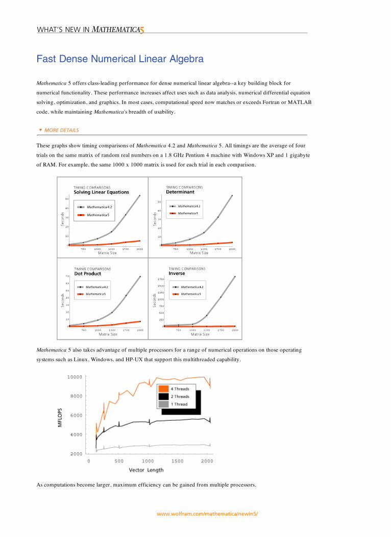
Mathematica 5 offers class-leading performance for dense numerical linear algebra--a key building block fornumerical functionality. These performance increases affect uses such as data analysis, numerical differential equationsolving, optimization, and graphics. In most cases, computational speed now matches or exceeds Fortran or MATLABcode, while maintaining Mathematica's breadth of usability.

These graphs show timing comparisons of Mathematica 4.2 and Mathematica 5. All timings are the average of fourtrials on the same matrix of random real numbers on a 1.8 GHz Pentium 4 machine with Windows XP and 1 gigabyteof RAM. For example, the same 1000 x 1000 matrix is used for each trial in each comparison.

Mathematica 5 also takes advantage of multiple processors for a range of numerical operations on those operatingsystems such as Linux, Windows, and HP-UX that support this multithreaded capability.

As computations become larger, maximum efficiency can be gained from multiple processors.

High-Speed Sparse Linear Algebra

Mathematica 5 utilizes specialized techniques to make computations involving sparse matrices (matrices in which mostof the elements are zero) vastly more efficient for large-scale problems. These improvements make Mathematicahighly suitable for large-scale simulations, optimization, or solving of partial or ordinary differential equations--allexamples in which sparse matrices are typically involved.

Mathematica 5's implementation of sparse linear algebra is unique because:

Symbolic preprocessing optimizes the formation of sparse matrices.

Sparse algorithms are automatically utilized where they would improve performance, without user intervention. (Theycan be manually evoked where required, too--for example, for comparison with traditional numerical systems.)

Any dimension (or rank) of array is handled.

The performance in speed and memory utilization of sparse linear algebra operations is on a par with, or better than,those in dedicated numerical systems.

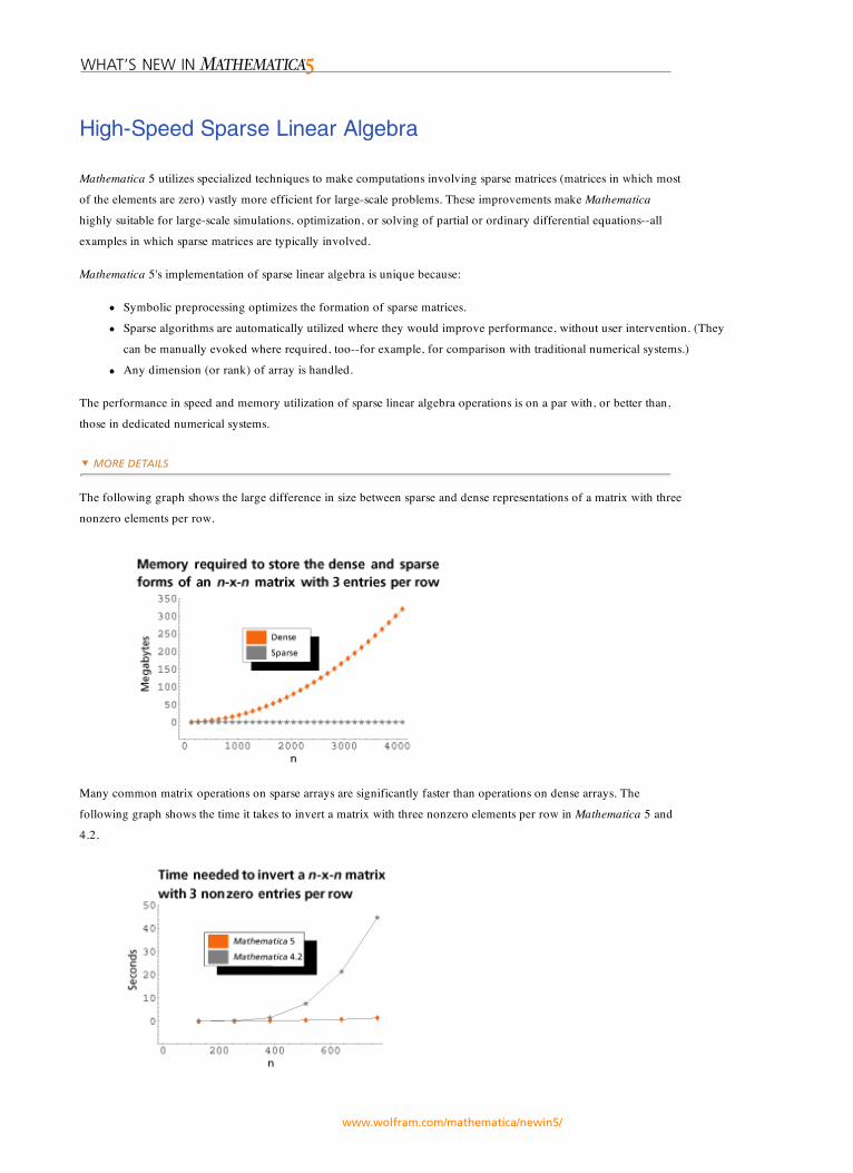
The following graph shows the large difference in size between sparse and dense representations of a matrix with threenonzero elements per row.

Many common matrix operations on sparse arrays are significantly faster than operations on dense arrays. Thefollowing graph shows the time it takes to invert a matrix with three nonzero elements per row in Mathematica 5 and4.2.

Large-Scale Linear Systems

Mathematica 5 is newly optimized for solving large-scale linear systems. It uses the efficient interior-point method,until now only available in costly special-purpose packages.

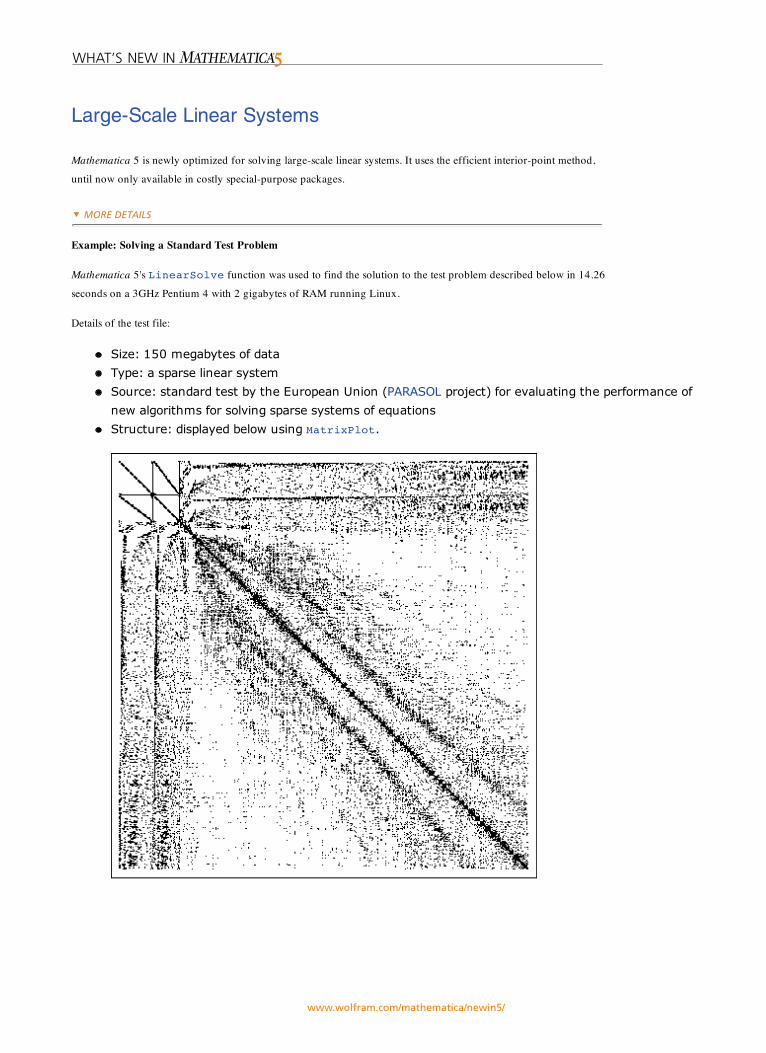
Example: Solving a Standard Test Problem

Mathematica 5's LinearSolve function was used to find the solution to the test problem described below in 14.26seconds on a 3GHz Pentium 4 with 2 gigabytes of RAM running Linux.

Details of the test file:

Size: 150 megabytes of data

Type: a sparse linear system

Source: standard test by the European Union (PARASOL project) for evaluating the performance of

new algorithms for solving sparse systems of equations

Structure: displayed below using MatrixPlot.

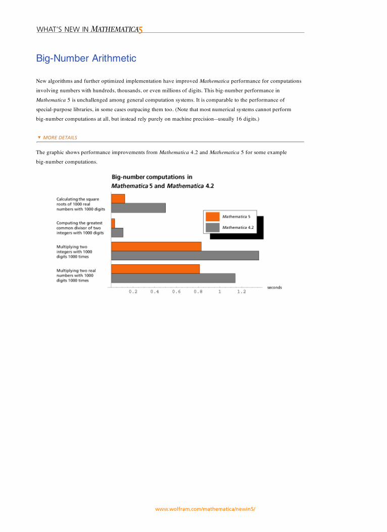
Big-Number Arithmetic

New algorithms and further optimized implementation have improved Mathematica performance for computationsinvolving numbers with hundreds, thousands, or even millions of digits. This big-number performance inMathematica 5 is unchallenged among general computation systems. It is comparable to the performance ofspecial-purpose libraries, in some cases outpacing them too. (Note that most numerical systems cannot performbig-number computations at all, but instead rely purely on machine precision--usually 16 digits.)

The graphic shows performance improvements from Mathematica 4.2 and Mathematica 5 for some examplebig-number computations.

64-Bit Platform Support

Mathematica 5 allows full access to nearly a million terabytes (billion gigabytes) of memory addressable on 64-bitmachines. 32-bit architectures and previous versions of Mathematica are limited to 4 gigabyte addressing. This limithas become significant in the increasingly large calculations now being run with Mathematica.

The combination of a 64-bit address space and fast numerics, part of Wolfram Research's gigaNumerics initiative, letsMathematica users solve very large problems.

Mathematica 5 is optimized for a large number of 64-bit CPUs and operating systems, including Sun Solaris forUltraSPARC, HP-UX for PA-RISC, IBM AIX for the Power architecture, HP Tru64 Unix on Alpha, Linux on Alpha,and SGI IRIX on MIPS. The two main benefits are the ability to solve vastly larger problems than on 32-bit platformsand the speed increases for big-number arithmetic due to the 64-bit word length.

This 64-bit optimization will also let Mathematica users take full advantage of planned performance increases in futureversions of these 64-bit processors.

Faster MathLink

Mathematica 5 uses optimized TCP/IP protocol for MathLink communication between front end and kernel, andbetween multiple kernels such as for gridMathematica deployments. These communications now occur at the speed ofthe underlying network.

The optimized TCP/IP protocol improves bandwidth by a factor of 10 and latency by a factor of 200 on a standard100Base-T network. With gigabit networks and crossbars found in leading-edge computing centers, the speed-ups areeven greater. Other changes--for example, a new shared memory protocol for Windows platforms--give a 10-foldimprovement for communication between parts of Mathematica on the same machine.

J/Link, .NET/Link, and most import and export formats rely on MathLink, thereby benefitting from performanceincreases in MathLink.

Numerical Solving of Differential Equations

The function NDSolve--the all-in-one numerical differential equation solver--has been completely rewritten.Performance has been significantly improved, new classes of equations can be solved, and the system willautomatically select between a wider range of methods to optimize the solution. Advanced users gain increased controlwith new capabilities for monitoring the progress of the solver, more options for evaluation and selection methods, aswell the ability to incorporate user-written custom solvers into NDSolve.

Some of the most significant improvements include:

More-efficient implementation leading to large speed increases for many types of differential

equations

NDSolve is now able to solve classes of differential-algebraic equations

New additional solving methods including explicit Runge-Kutta methods, implicit Runge-Kutta

methods of arbitrary order, and extrapolation methods

NDSolve is now able to solve (n+1)-dimensional partial differential equations

NDSolve now supports vector and array variables

New options EvaluationMonitor and StepMonitor allow monitoring of the progress of the solution

and more fine-tuning of the solving procedure

A new framework for inclusion of user-defined methods

Additional advanced documentation covering applications, methods, and options of NDSolve

NDSolve chooses the appropriate method automatically, according to problem type. It will also change methodsduring the evaluation process if appropriate--for example, if an equation goes from stiff to non-stiff or vice versa.

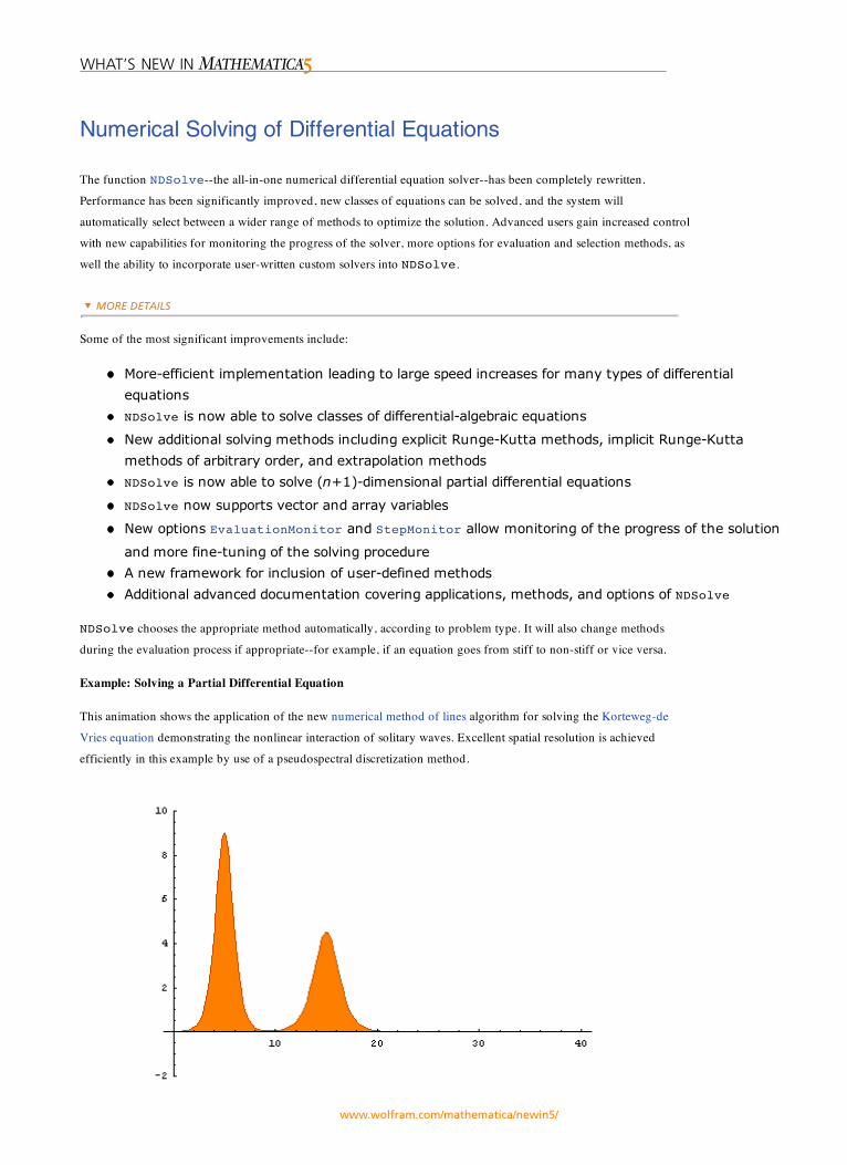
Example: Solving a Partial Differential Equation

This animation shows the application of the new numerical method of lines algorithm for solving the Korteweg-deVries equation demonstrating the nonlinear interaction of solitary waves. Excellent spatial resolution is achievedefficiently in this example by use of a pseudospectral discretization method.

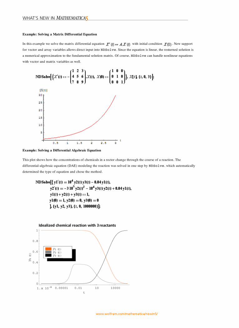
Example: Solving a Matrix Differential Equation

In this example we solve the matrix differential equation with initial condition . New supportfor vector and array variables allows direct input into NDSolve. Since the equation is linear, the resturned solution isa numerical approximation to the fundamental solution matrix. Of course, NDSolve can handle nonlinear equationswith vector and matrix variables as well.

Example: Solving a Differential Algebraic Equation

This plot shows how the concentrations of chemicals in a rector change through the course of a reaction. Thedifferential-algebraic equation (DAE) modeling the reaction was solved in one step by NDSolve, which automaticallydetermined the type of equation and chose the method.

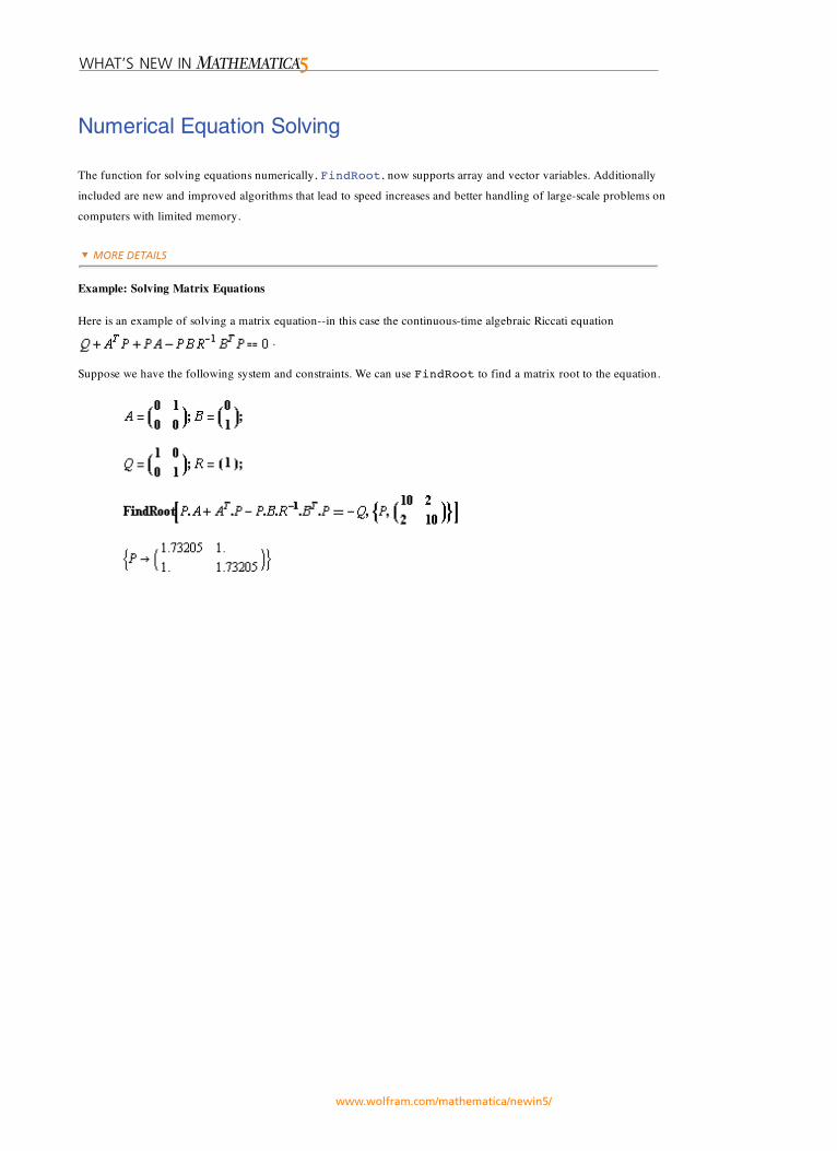
Numerical Equation Solving

The function for solving equations numerically, FindRoot, now supports array and vector variables. Additionallyincluded are new and improved algorithms that lead to speed increases and better handling of large-scale problems oncomputers with limited memory.

Example: Solving Matrix Equations

Here is an example of solving a matrix equation--in this case the continuous-time algebraic Riccati equation .

Suppose we have the following system and constraints. We can use FindRoot to find a matrix root to the equation.

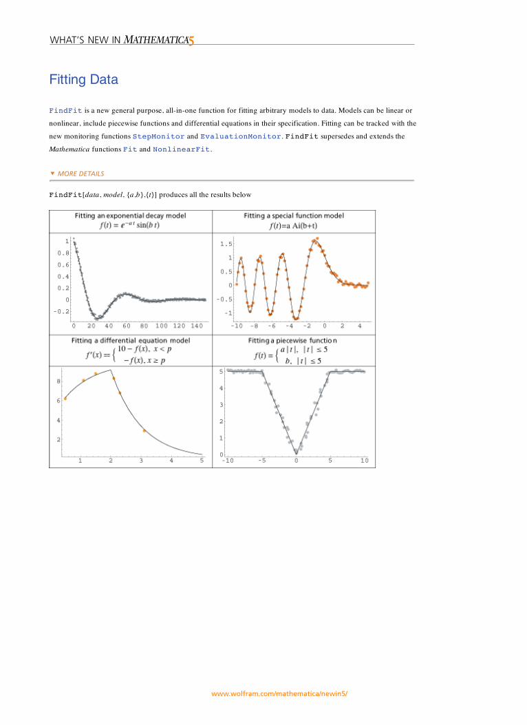
Fitting Data

FindFit is a new general purpose, all-in-one function for fitting arbitrary models to data. Models can be linear or nonlinear, include piecewise functions and differential equations in their specification. Fitting can be tracked with thenew monitoring functions StepMonitor and EvaluationMonitor. FindFit supersedes and extends theMathematica functions Fit and NonlinearFit.

FindFit[data, model, {a,b},{t}] produces all the results below

DSolve

The symbolic differential equation solver DSolve has been extended. Key new features include solving classes of

mixed systems of differential and algebraic equations (DAEs), and the ability to find all rational solutions to systems of

linear differential equations with rational coefficients.

Example: Solving differential-algebraic equations

The solution to the following differential-algebraic equation is fully specified by only one initial value because of the

algebraic equation between the variables x(t) and y(t).

Example: Linear System with Rational Function Coefficients

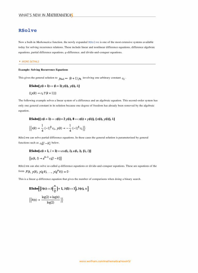
RSolve

Now a built-in Mathematica function, the newly expanded RSolve is one of the most extensive systems available

today for solving recurrence relations. These include linear and nonlinear difference equations, difference algebraic

equations, partial difference equations, q-difference, and divide-and-conquer equations.

Example: Solving Recurrence Equations

This gives the general solution to involving one arbitrary constant .

The following example solves a linear system of a difference and an algebraic equation. This second-order system has

only one general constant in its solution because one degree of freedom has already been removed by the algebraic

equation.

RSolve can solve partial difference equations. In these cases the general solution is parameterized by general

functions such as below.

RSolve can also solve so-called q-difference equations or divide-and-conquer equations. These are equations of the

form .

This is a linear q-difference equation that gives the number of comparisons when doing a binary search.

Reduce

The function Reduce has been extended to solve any combination of equalities, inequalities, existential quantifiers,

universal quantifiers, and domain specifications, making it the most comprehensive symbolic solving function

available today. Automatic switching of algorithms is utilized extensively to achieve the range of capabilities available

with Reduce.

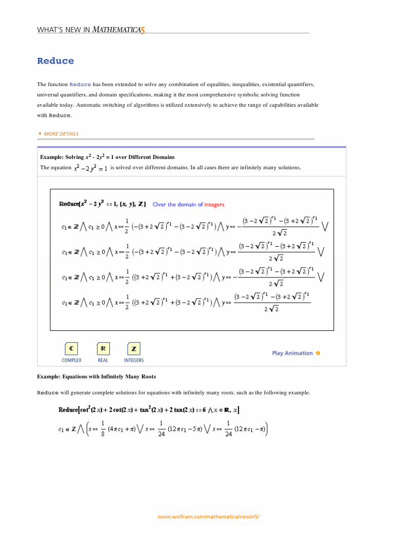
Example: Solving x2 - 2y2 = 1 over Different Domains

The equation is solved over different domains. In all cases there are infinitely many solutions.

Example: Equations with Infinitely Many Roots

Reduce will generate complete solutions for equations with infinitely many roots. such as the following example.

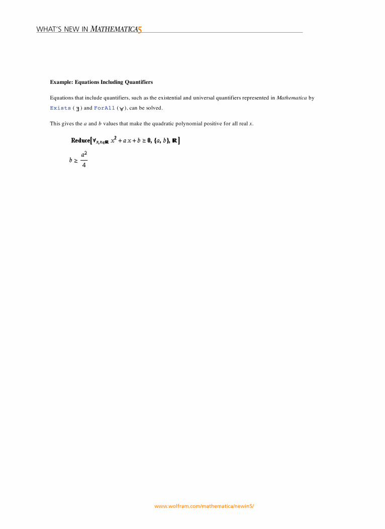
Example: Equations Including Quantifiers

Equations that include quantifiers, such as the existential and universal quantifiers represented in Mathematica by

Exists ( ) and ForAll ( ), can be solved.

This gives the a and b values that make the quadratic polynomial positive for all real x.

Resolve

The function Resolve can eliminate quantifiers (for example and ) from arbitrary polynomial systems in

complex or real variables using the same methods used by the solving function Reduce. For cases in which obtaining

an implicit quantifier-free form of the system is easier than computing explicit solutions, Resolve returns the implicit

form. Resolve can also eliminate quantifiers involving Boolean variables.

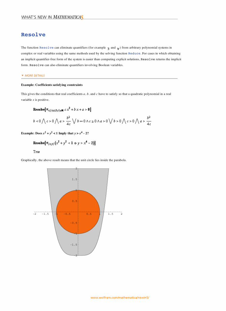
Example: Coefficients satisfying constraints

This gives the conditions that real coefficients a, b, and c have to satisfy so that a quadratic polynomial in a real

variable x is positive.

Example: Does x2 + y2 < 1 Imply that y > x4 - 2?

Graphically, the above result means that the unit circle lies inside the parabola.

FindInstance

The new function FindInstance gives, at most, the requested number of different numerical solutions to an

equation or inequality. For problems in which the complete solution is not needed, finding instances of solutions can

be much faster than trying to find the whole solution set. FindInstance works for all problems that Reduce can

solve fully. It can also find instances for some problems that Reduce cannot solve.

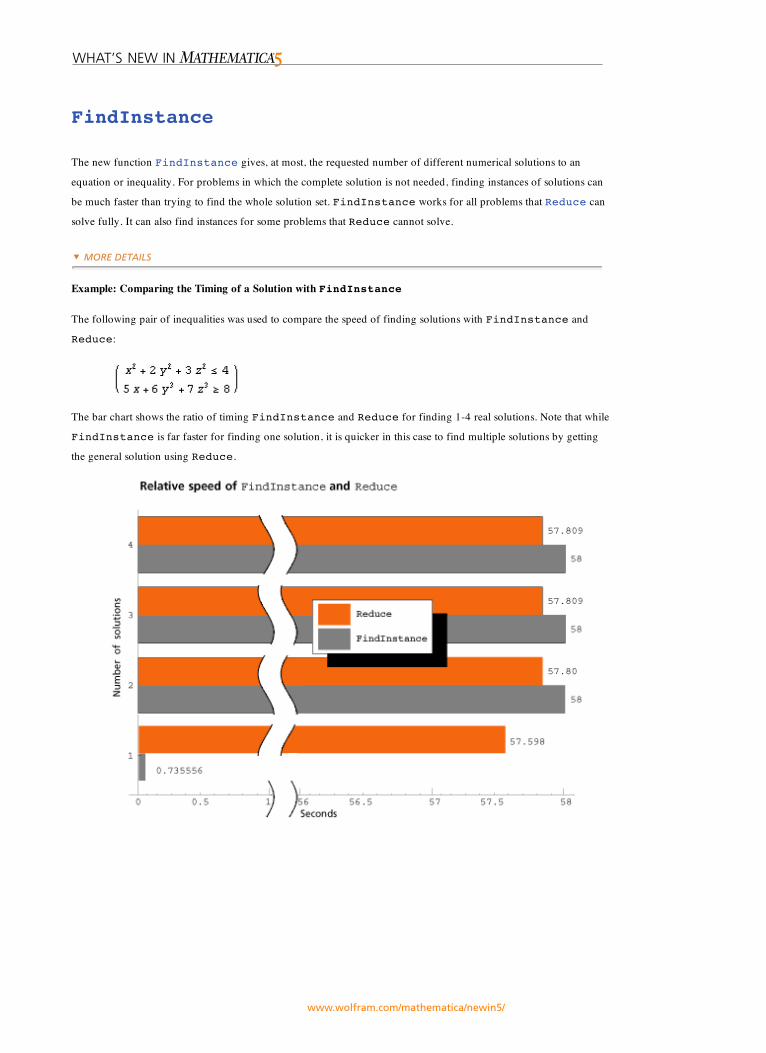
Example: Comparing the Timing of a Solution with FindInstance

The following pair of inequalities was used to compare the speed of finding solutions with FindInstance and

Reduce:

The bar chart shows the ratio of timing FindInstance and Reduce for finding 1-4 real solutions. Note that while

FindInstance is far faster for finding one solution, it is quicker in this case to find multiple solutions by getting

the general solution using Reduce.

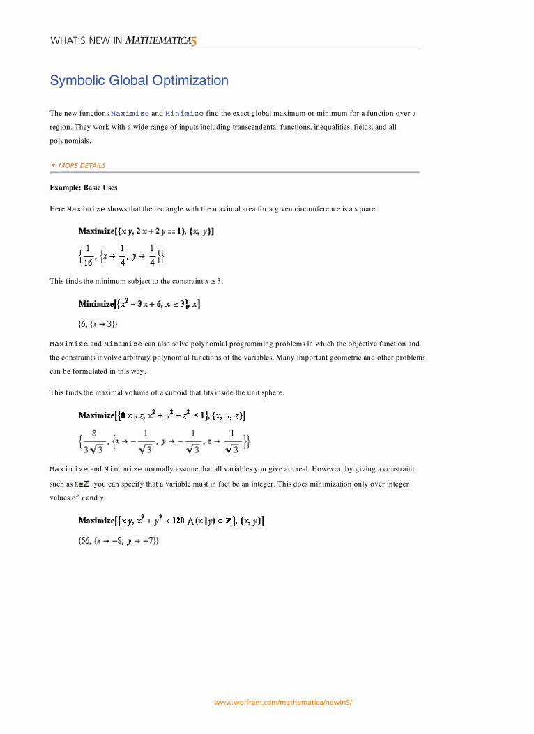
Symbolic Global Optimization

The new functions Maximize and Minimize find the exact global maximum or minimum for a function over a

region. They work with a wide range of inputs including transcendental functions, inequalities, fields, and all

polynomials.

Example: Basic Uses

Here Maximize shows that the rectangle with the maximal area for a given circumference is a square.

This finds the minimum subject to the constraint x ≥ 3.

Maximize and Minimize can also solve polynomial programming problems in which the objective function and

the constraints involve arbitrary polynomial functions of the variables. Many important geometric and other problems

can be formulated in this way.

This finds the maximal volume of a cuboid that fits inside the unit sphere.

Maximize and Minimize normally assume that all variables you give are real. However, by giving a constraint

such as , you can specify that a variable must in fact be an integer. This does minimization only over integer

values of x and y.

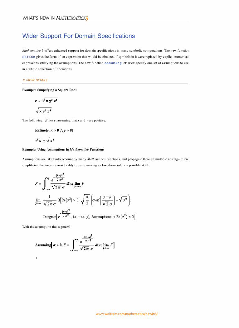
Wider Support For Domain Specifications

Mathematica 5 offers enhanced support for domain specifications in many symbolic computations. The new function

Refine gives the form of an expression that would be obtained if symbols in it were replaced by explicit numerical

expressions satisfying the assumptions. The new function Assuming lets users specify one set of assumptions to use

in a whole collection of operations.

Example: Simplifying a Square Root

The following refines e, assuming that x and y are positive.

Example: Using Assumptions in Mathematica Functions

Assumptions are taken into account by many Mathematica functions, and propagate through multiple nesting--often

simplifying the answer considerably or even making a close-form solution possible at all.

With the assumption that sigma=0

Importing and Exporting

Mathematica 5 continues to enhance the capabilities of Import and Export to cover the widest range of data

formats and work with large datasets. SVG, PNG, and DICOM are among the graphics, web and matrix formats added,

bringing the total number to over 40.

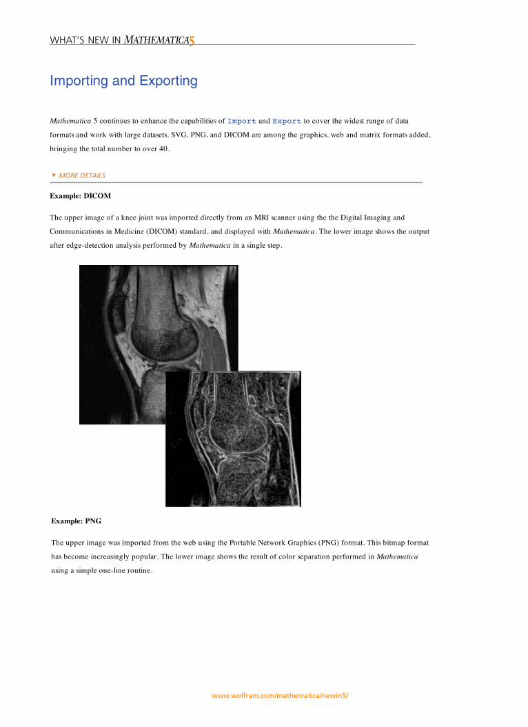
Example: DICOM

The upper image of a knee joint was imported directly from an MRI scanner using the the Digital Imaging and

Communications in Medicine (DICOM) standard, and displayed with Mathematica. The lower image shows the output

after edge-detection analysis performed by Mathematica in a single step.

Example: PNG

The upper image was imported from the web using the Portable Network Graphics (PNG) format. This bitmap format

has become increasingly popular. The lower image shows the result of color separation performed in Mathematica

using a simple one-line routine.

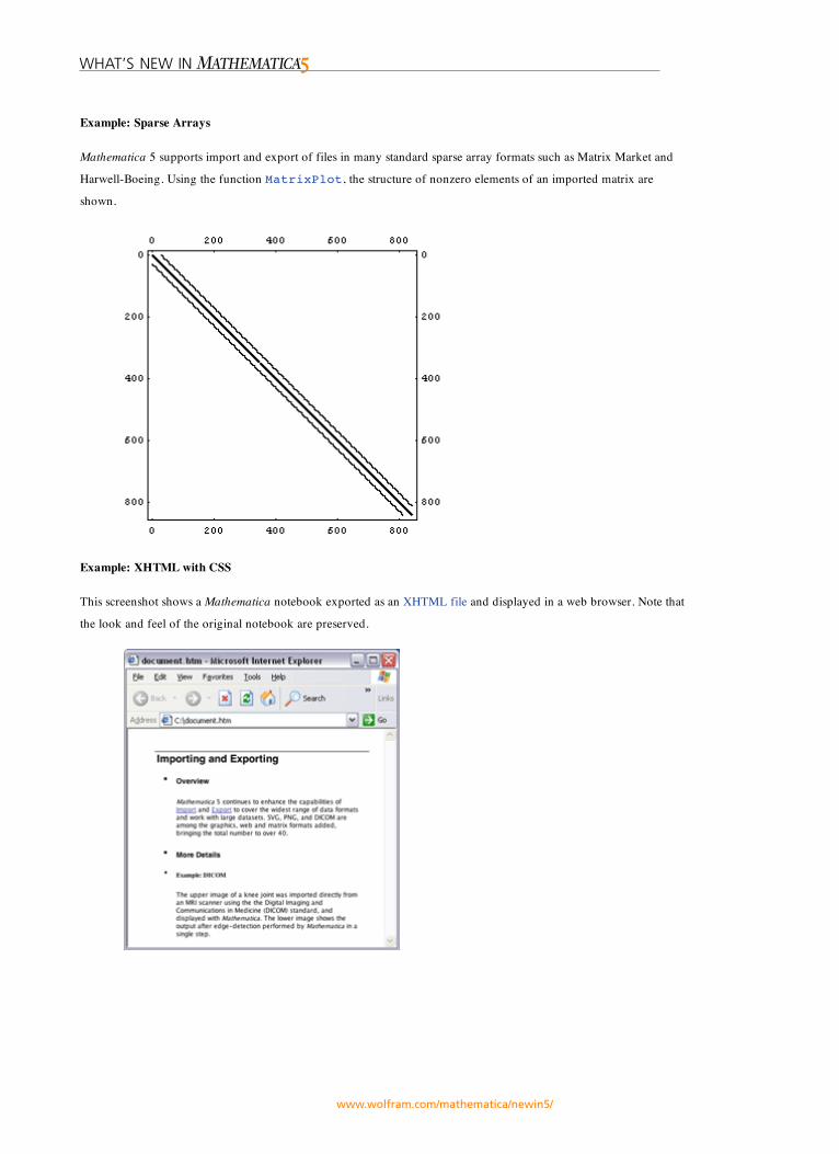
Example: Sparse Arrays

Mathematica 5 supports import and export of files in many standard sparse array formats such as Matrix Market and

Harwell-Boeing. Using the function MatrixPlot, the structure of nonzero elements of an imported matrix are

shown.

Example: XHTML with CSS

This screenshot shows a Mathematica notebook exported as an XHTML file and displayed in a web browser. Note that

the look and feel of the original notebook are preserved.

Connection Technology

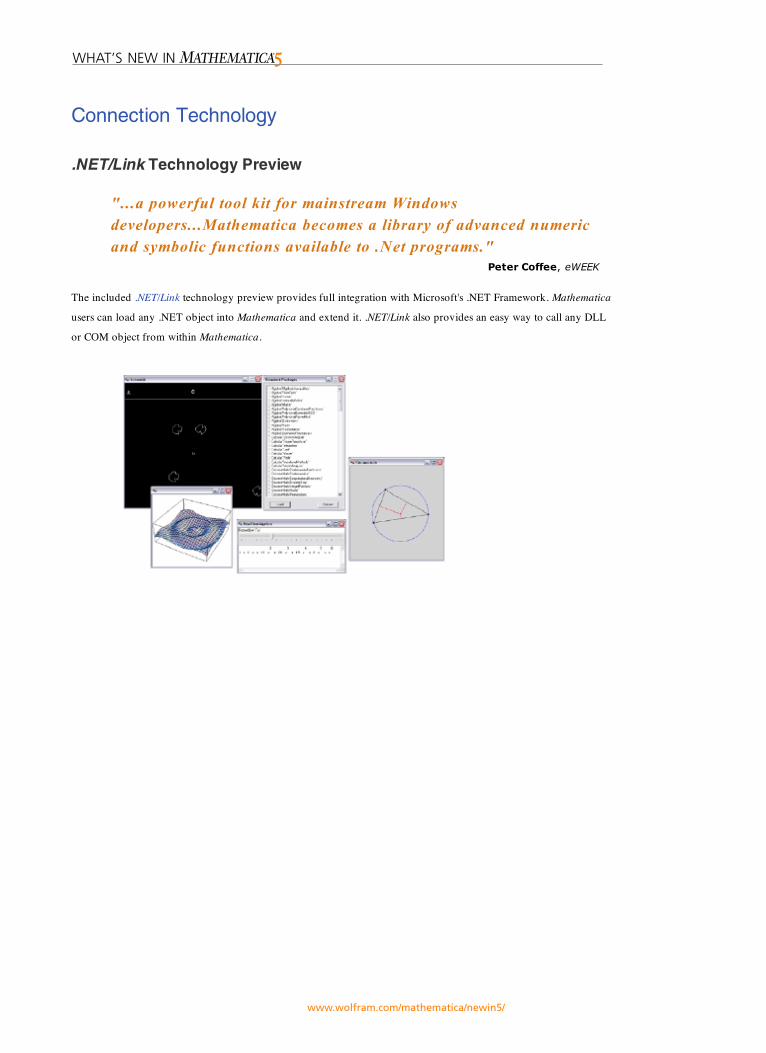
.NET/Link Technology Preview

"...a powerful tool kit for mainstream Windows developers...Mathematica becomes a library of advanced numericand symbolic functions available to .Net programs."

Peter Coffee, eWEEK

The included .NET/Link technology preview provides full integration with Microsoft's .NET Framework. Mathematica

users can load any .NET object into Mathematica and extend it. .NET/Link also provides an easy way to call any DLL

or COM object from within Mathematica.

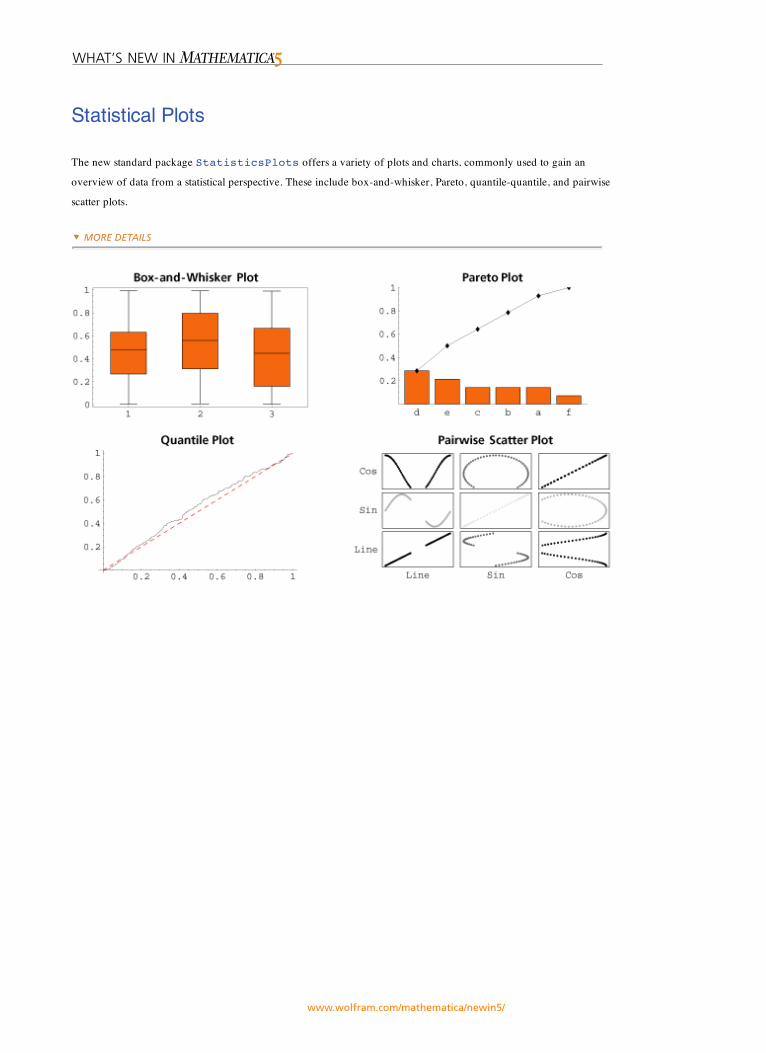
Statistical Plots

The new standard package StatisticsPlots offers a variety of plots and charts, commonly used to gain an

overview of data from a statistical perspective. These include box-and-whisker, Pareto, quantile-quantile, and pairwise

scatter plots.

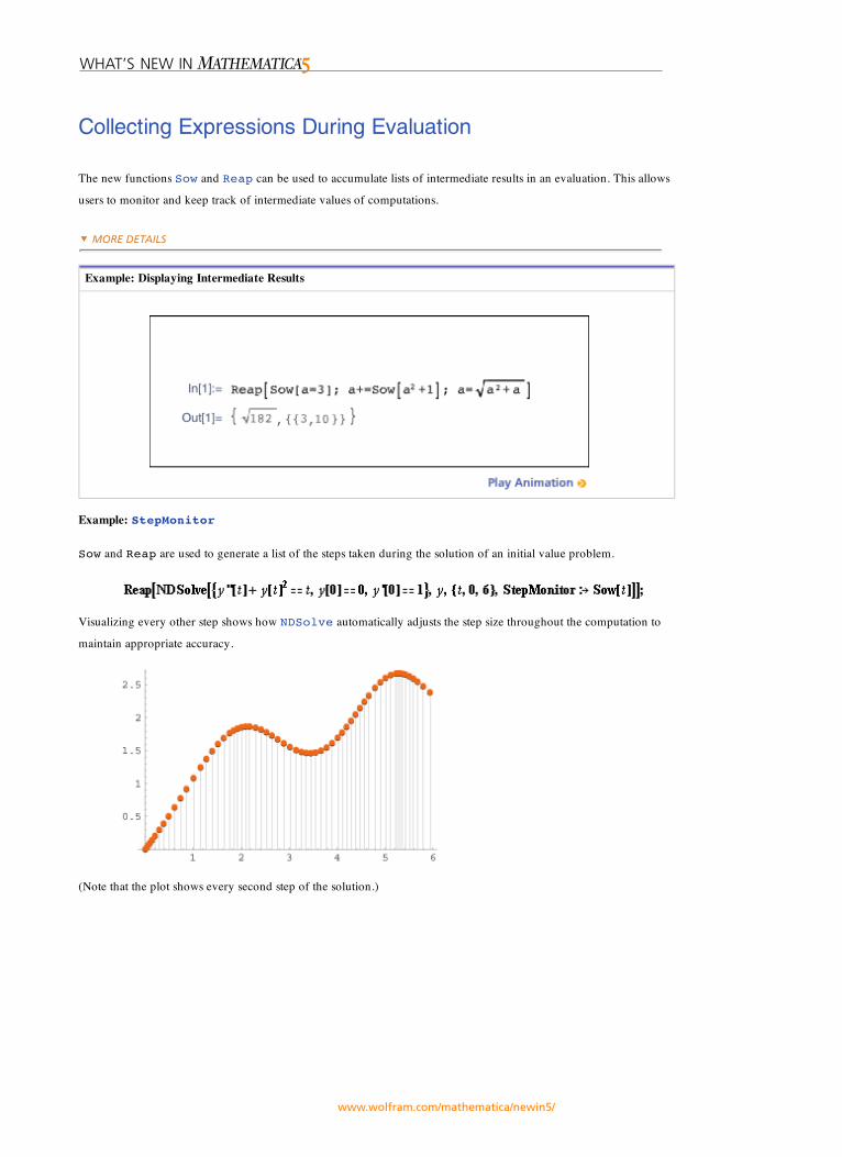
Collecting Expressions During Evaluation

The new functions Sow and Reap can be used to accumulate lists of intermediate results in an evaluation. This allows

users to monitor and keep track of intermediate values of computations.

Example: Displaying Intermediate Results

Example: StepMonitor

Sow and Reap are used to generate a list of the steps taken during the solution of an initial value problem.

Visualizing every other step shows how NDSolve automatically adjusts the step size throughout the computation to

maintain appropriate accuracy.

(Note that the plot shows every second step of the solution.)

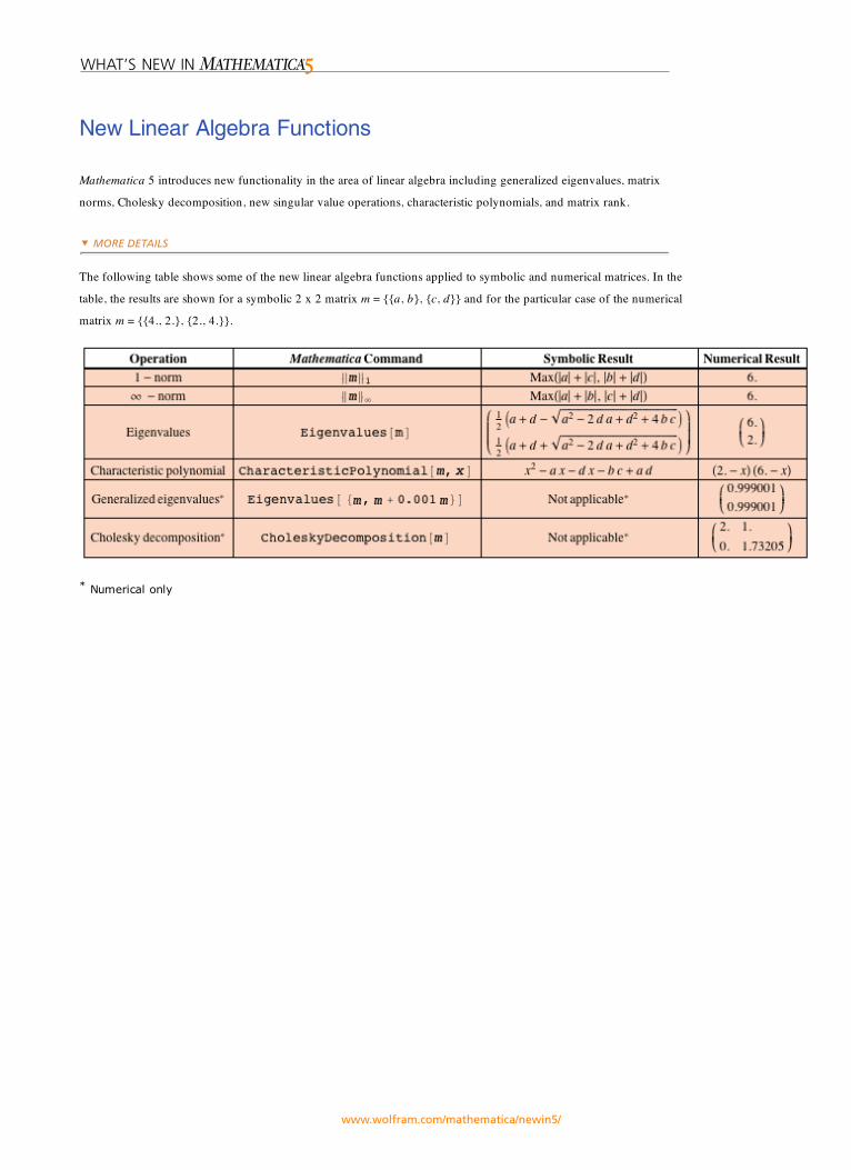
New Linear Algebra Functions

Mathematica 5 introduces new functionality in the area of linear algebra including generalized eigenvalues, matrix

norms, Cholesky decomposition, new singular value operations, characteristic polynomials, and matrix rank.

The following table shows some of the new linear algebra functions applied to symbolic and numerical matrices. In the

table, the results are shown for a symbolic 2 x 2 matrix m = {{a, b}, {c, d}} and for the particular case of the numerical

matrix m = {{4., 2.}, {2., 4.}}.

* Numerical only

Algebraic Number Objects

Mathematica 5 brings high-performance algebraic number arithmetic within specified algebraic number fields.

Mathematica has been providing representation of algebraic numbers as Root objects since Version 3. A Root object

contains the minimal polynomial of the algebraic number and the root number--an integer indicating which of the

roots of the minimal polynomial the Root object represents. This allows for unique representation of arbitrary

complex algebraic numbers.

A disadvantage is that performing arithmetic operations in this representation is costly. If we restrict ourselves to

computations within a fixed finite algebraic extension, , of rationals, we can use a more convenient representation

of elements of , namely as polynomials in . Within a fixed algebraic number field, the algebraic number

arithmetic in the Algebraic object representation is much faster than in the Root object representation.

Mathematica 5 contains extensive functionality related to algebraic number fields, available through the package

NumberTheory`AlgebraicNumberFields`.

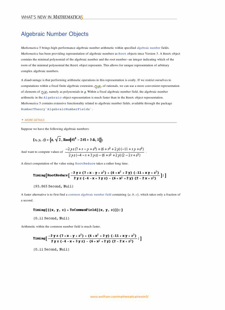
Suppose we have the following algebraic numbers:

And want to compute values of .

A direct computation of the value using RootReduce takes a rather long time.

A faster alternative is to first find a common algebraic number field containing {a, b, c}, which takes only a fraction of

a second.

Arithmetic within the common number field is much faster.

Authoring and Presentation

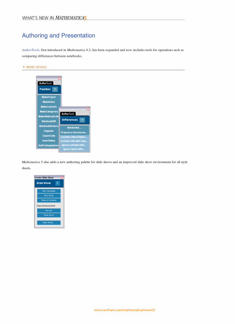
AuthorTools, first introduced in Mathematica 4.2, has been expanded and now includes tools for operations such as

comparing differences between notebooks.

Mathematica 5 also adds a new authoring palette for slide shows and an improved slide show environment for all style

sheets.