Beginning biomolecular structure analysis with Bio3D:PDB structure manipulation and analysis

Lars Skjaerven, Xin-Qiu Yao & Barry J. GrantFebruary 12, 2015

Contents

Introduction 2

New to R? . . . . . . . . . . . . . . . . . . . . . . . . . . . . . . . . . . . . . . . . . . . . . 2

Using this vignette . . . . . . . . . . . . . . . . . . . . . . . . . . . . . . . . . . . . . . . . 2

1 Getting started 2

1.1 Bio3D functions and their typical usage . . . . . . . . . . . . . . . . . . . . . . . . . 3

2 Working with individual PDB files 3

2.1 Read a PDB file . . . . . . . . . . . . . . . . . . . . . . . . . . . . . . . . . . . . . . 3

2.2 Atom selection . . . . . . . . . . . . . . . . . . . . . . . . . . . . . . . . . . . . . . . 7

2.3 Write a PDB object . . . . . . . . . . . . . . . . . . . . . . . . . . . . . . . . . . . . 10

2.4 Manipulate a PDB object . . . . . . . . . . . . . . . . . . . . . . . . . . . . . . . . . 11

2.5 Concatenate multiple PDBs . . . . . . . . . . . . . . . . . . . . . . . . . . . . . . . . 12

2.6 Coordinate superposition and structural alignment . . . . . . . . . . . . . . . . . . . 12

2.7 Binding site identification . . . . . . . . . . . . . . . . . . . . . . . . . . . . . . . . . 15

2.8 Reading multi-model PDB files . . . . . . . . . . . . . . . . . . . . . . . . . . . . . . 16

2.9 Identification of dynamic domains . . . . . . . . . . . . . . . . . . . . . . . . . . . . 18

2.10 Invariant core identification . . . . . . . . . . . . . . . . . . . . . . . . . . . . . . . . 18

3 Constructing biological units 21

4 Working with multiple PDB files 25

5 Where to next 29

Document and current Bio3D session details 29

References 30

1

Introduction

Bio3D1 is an R package containing utilities for the analysis of biomolecular structure, sequence andtrajectory data (Grant et al. 2006, Skjaerven et al. (2015)). Features include the ability to read andwrite biomolecular structure, sequence and dynamic trajectory data, perform atom selection, re-orientation, superposition, rigid core identification, clustering, distance matrix analysis, conservationanalysis, normal mode analysis and principal component analysis. Bio3D takes advantage of theextensive graphical and statistical capabilities of the R environment and thus represents a usefulframework for exploratory analysis of structural data.

New to R?

There are numerous on–line resources that can help you get started using R effectively. A numberof these can be found from the main R website at http://www.r-project.org. We particularly likethe following:

• Try R: an interactive R tutorial in your web browser• An introduction to R: The offical R manual• Learn R: Learn by doing in your web browser (requires free registration)

Using this vignette

The aim of this document, termed a vignette2 in R parlance, is to provide a brief introduction toPDB structure manipulation and analysis with Bio3D. A number of other Bio3D package vignettesand tutorals are available online at http://thegrantlab.org/bio3d/tutorials. In particular, detailedinstructions for obtaining and installing the Bio3D package on various platforms can be found inthe Installing Bio3D Vignette. Note that this vignette was generated using Bio3D version 2.2.0.

1 Getting started

Start R (type R at the command prompt or, on Windows, double click on the R icon) and load theBio3D package by typing library(bio3d) at the R console prompt.

library(bio3d)

Then use the command lbio3d() or help(package=bio3d) to list the functions within the packageand help(FunctionName) to obtain more information about an individual function.

# List of bio3d functions with brief descriptionhelp(package=bio3d)

# Detailed help on a particular function, e.g. ’pca.xyz’help(pca.xyz)

1The latest version of the package, full documentation and further vignettes (including detailed installationinstructions) can be obtained from the main Bio3D website: thegrantlab.org/bio3d/.

2This vignette contains executable examples, see help(vignette) for further details.

2

To search the help system for documentation matching a particular word or topic use the commandhelp.search("topic"). For example, help.search("pdb")

help.search("pdb")

Typing help.start() will start a local HTML interface to the R documentation and help system.After initiating help.start() in a session the help() commands will open as HTML pages in yourweb browser.

1.1 Bio3D functions and their typical usage

The Bio3D package consists of input/output functions, conversion and manipulation functions,analysis functions, and graphics functions all of which are fully documented both online and withinthe R help system introduced above.

To better understand how a particular function operates it is often helpful to view and execute anexample. Every function within the Bio3D package is documented with example code that you canview by issuing the help() command.

Running the command example(function) will directly execute the example for a given function.In addition, a number of longer worked examples are available as Tutorials on the Bio3D website.

example(plot.bio3d)

2 Working with individual PDB files

Protein Data Bank files (or PDB files) are the most common format for the distribution andstorage of high-resolution biomolecular coordinate data. The Bio3D package contains functionsfor the reading (read.pdb(), read.fasta.pdb(), get.pdb(), convert.pdb(), basename.pdb()),writing (write.pdb()) and manipulation (trim.pdb(), cat.pdb(), pdbsplit(), atom.select(),pdbseq()) of PDB files. Indeed numerous Bio3D analysis functions are intended to operate onPDB file derived data (e.g. blast.pdb(), chain.pdb(), nma.pdb(), pdb.annotate(), pdbaln(),pdbfit(), struct.aln(), dssp(), pca.pdbs() etc.)

At their most basic, PDB coordinate files contain a list of all the atoms of one or more molecularstructures. Each atom position is defined by its x, y, z coordinates in a conventional orthogonalcoordinate system. Additional data, including listings of observed secondary structure elements, arealso commonly (but not always) detailed in PDB files.

2.1 Read a PDB file

To read a single PDB file with Bio3D we can use the read.pdb() function. The minimal inputrequired for this function is a specification of the file to be read. This can be either the file nameof a local file on disc or the RCSB PDB identifier of a file to read directly from the on-line PDBrepository. For example to read and inspect the on-line file with PDB ID 4q21:

3

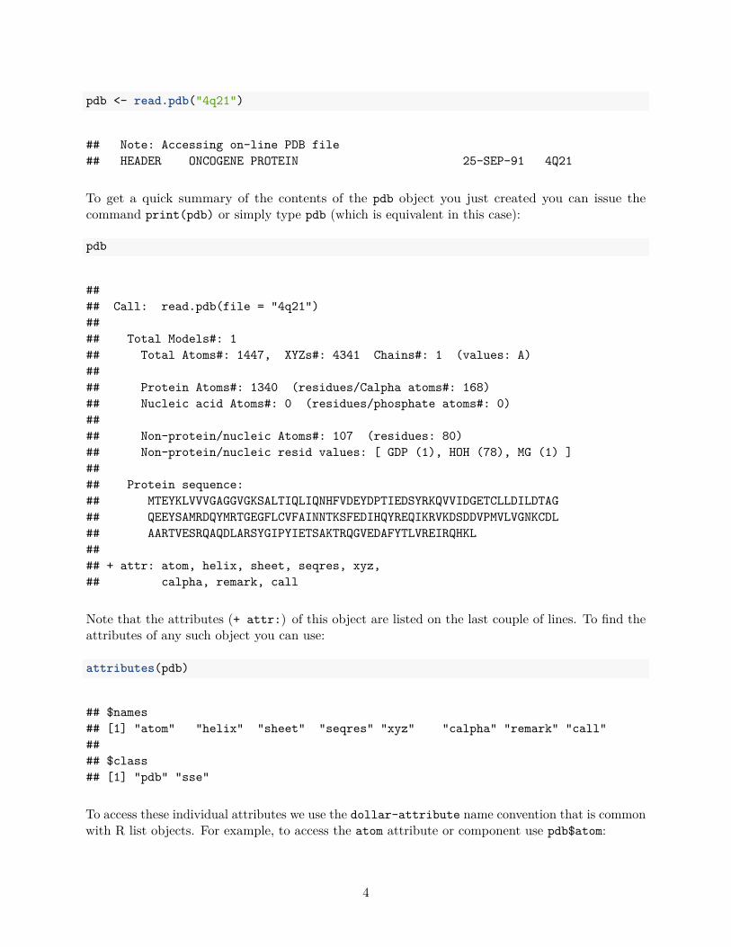
pdb <- read.pdb("4q21")

## Note: Accessing on-line PDB file## HEADER ONCOGENE PROTEIN 25-SEP-91 4Q21

To get a quick summary of the contents of the pdb object you just created you can issue thecommand print(pdb) or simply type pdb (which is equivalent in this case):

pdb

#### Call: read.pdb(file = "4q21")#### Total Models#: 1## Total Atoms#: 1447, XYZs#: 4341 Chains#: 1 (values: A)#### Protein Atoms#: 1340 (residues/Calpha atoms#: 168)## Nucleic acid Atoms#: 0 (residues/phosphate atoms#: 0)#### Non-protein/nucleic Atoms#: 107 (residues: 80)## Non-protein/nucleic resid values: [ GDP (1), HOH (78), MG (1) ]#### Protein sequence:## MTEYKLVVVGAGGVGKSALTIQLIQNHFVDEYDPTIEDSYRKQVVIDGETCLLDILDTAG## QEEYSAMRDQYMRTGEGFLCVFAINNTKSFEDIHQYREQIKRVKDSDDVPMVLVGNKCDL## AARTVESRQAQDLARSYGIPYIETSAKTRQGVEDAFYTLVREIRQHKL#### + attr: atom, helix, sheet, seqres, xyz,## calpha, remark, call

Note that the attributes (+ attr:) of this object are listed on the last couple of lines. To find theattributes of any such object you can use:

attributes(pdb)

## $names## [1] "atom" "helix" "sheet" "seqres" "xyz" "calpha" "remark" "call"#### $class## [1] "pdb" "sse"

To access these individual attributes we use the dollar-attribute name convention that is commonwith R list objects. For example, to access the atom attribute or component use pdb$atom:

4

head(pdb$atom)

## type eleno elety alt resid chain resno insert x y z o## 1 ATOM 1 N <NA> MET A 1 <NA> 64.080 50.529 32.509 1## 2 ATOM 2 CA <NA> MET A 1 <NA> 64.044 51.615 33.423 1## 3 ATOM 3 C <NA> MET A 1 <NA> 63.722 52.849 32.671 1## 4 ATOM 4 O <NA> MET A 1 <NA> 64.359 53.119 31.662 1## 5 ATOM 5 CB <NA> MET A 1 <NA> 65.373 51.805 34.158 1## 6 ATOM 6 CG <NA> MET A 1 <NA> 65.122 52.780 35.269 1## b segid elesy charge## 1 28.66 <NA> N <NA>## 2 29.19 <NA> C <NA>## 3 30.27 <NA> C <NA>## 4 34.93 <NA> O <NA>## 5 28.49 <NA> C <NA>## 6 32.18 <NA> C <NA>

# Print $atom data for the first two atomspdb$atom[1:2, ]

## type eleno elety alt resid chain resno insert x y z o## 1 ATOM 1 N <NA> MET A 1 <NA> 64.080 50.529 32.509 1## 2 ATOM 2 CA <NA> MET A 1 <NA> 64.044 51.615 33.423 1## b segid elesy charge## 1 28.66 <NA> N <NA>## 2 29.19 <NA> C <NA>

# Print a subset of $atom data for the first two atomspdb$atom[1:2, c("eleno", "elety", "x","y","z")]

## eleno elety x y z## 1 1 N 64.080 50.529 32.509## 2 2 CA 64.044 51.615 33.423

# Note that individual $atom records can also be accessed like thispdb$atom$elety[1:2]

## [1] "N" "CA"

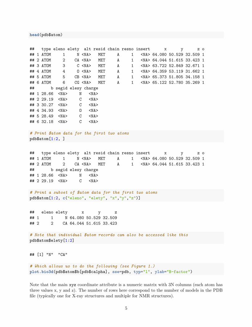
# Which allows us to do the following (see Figure 1.)plot.bio3d(pdb$atom$b[pdb$calpha], sse=pdb, typ="l", ylab="B-factor")

Note that the main xyz coordinate attribute is a numeric matrix with 3N columns (each atom hasthree values x, y and z). The number of rows here correspond to the number of models in the PDBfile (typically one for X-ray structures and multiple for NMR structures).

5

020

4060

1 50 100 150

Residue

B−

fact

or

Figure 1: Residue temperature factors for PDB ID 4q21 with secondary structure element (SSE)annotation in marginal regions plotted with function plot.bio3d()

# Print a summary of the coordinate data in $xyzpdb$xyz

#### Total Frames#: 1## Total XYZs#: 4341, (Atoms#: 1447)#### [1] 64.08 50.529 32.509 <...> 74.159 76.923 41.999 [4341]#### + attr: Matrix DIM = 1 x 4341

# Examine the row and column dimensionsdim(pdb$xyz)

## [1] 1 4341

pdb$xyz[ 1, atom2xyz(1:2) ]

## [1] 64.080 50.529 32.509 64.044 51.615 33.423

6

Side-note: The ‘pdb’ class Objects created by the read.pdb() function are of class “pdb”.This is recognized by other so called generic Bio3D functions (for example atom.select(), nma(),print(), summary() etc.). A generic function is a function that examines the class of its firstargument, and then decides what type of operation to perform (more specifically it decides whichspecific method to dispatch to). So for example, the generic atom.select() function knows thatthe input is of class “pdb”, rather than for example an AMBER parameter and topology file, andwill act accordingly.

A careful reader will also of noted that our “pdb” object created above also has a second class,namely “sse” (see the output of attributes(pdb) or class(pdb)). This stands for secondarystructure elements and is recognized by the plot.bio3d() function to annotate the positions ofmajor secondary structure elements in the marginal regions of these plots (see Figure 1). This is allpart of the R S3 object orientation system. This S3 system os used throughout Bio3D to simplifyand facilitate our work with these types of objects.

2.2 Atom selection

The Bio3D atom.select() function is arguably one of the most challenging for newcomers to master.It is however central to PDB structure manipulation and analysis. At its most basic, this functionoperates on PDB structure objects (as created by read.pdb()) and returns the numeric indices ofa selected atom subset. These indices can then be used to access the $atom and $xyz attributes ofPDB structure related objects.

For example to select the indices for all C-alpha atoms we can use the following command:

# Select all C-alpha atoms (return their indices)ca.inds <- atom.select(pdb, "calpha")ca.inds

#### Call: atom.select.pdb(pdb = pdb, string = "calpha")#### Atom Indices#: 168 ($atom)## XYZ Indices#: 504 ($xyz)#### + attr: atom, xyz, call

Note that the attributes of the returned ca.inds from atom.select() include both atom and xyzcomponents. These are numeric vectors that can be used as indices to access the correspondingatom and xyz components of the input PDB structure object. For example:

# Print details of the first few selected atomshead( pdb$atom[ca.inds$atom, ] )

## type eleno elety alt resid chain resno insert x y z o## 2 ATOM 2 CA <NA> MET A 1 <NA> 64.044 51.615 33.423 1## 10 ATOM 10 CA <NA> THR A 2 <NA> 62.439 54.794 32.359 1

7

## 17 ATOM 17 CA <NA> GLU A 3 <NA> 63.968 58.232 32.801 1## 26 ATOM 26 CA <NA> TYR A 4 <NA> 61.817 61.333 33.161 1## 38 ATOM 38 CA <NA> LYS A 5 <NA> 63.343 64.814 33.163 1## 47 ATOM 47 CA <NA> LEU A 6 <NA> 61.321 67.068 35.557 1## b segid elesy charge## 2 29.19 <NA> C <NA>## 10 28.10 <NA> C <NA>## 17 30.95 <NA> C <NA>## 26 23.42 <NA> C <NA>## 38 21.34 <NA> C <NA>## 47 18.99 <NA> C <NA>

# And selected xyz coordinateshead( pdb$xyz[, ca.inds$xyz] )

## [1] 64.044 51.615 33.423 62.439 54.794 32.359

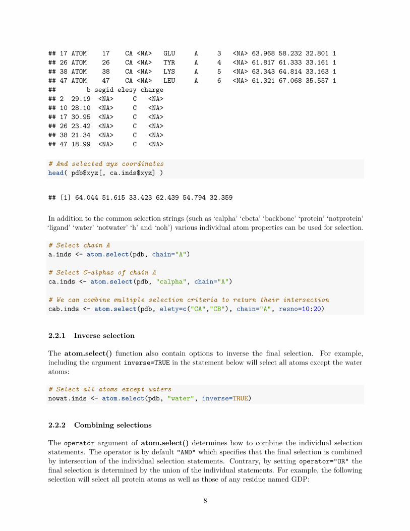
In addition to the common selection strings (such as ‘calpha’ ‘cbeta’ ‘backbone’ ‘protein’ ‘notprotein’‘ligand’ ‘water’ ‘notwater’ ‘h’ and ‘noh’) various individual atom properties can be used for selection.

# Select chain Aa.inds <- atom.select(pdb, chain="A")

# Select C-alphas of chain Aca.inds <- atom.select(pdb, "calpha", chain="A")

# We can combine multiple selection criteria to return their intersectioncab.inds <- atom.select(pdb, elety=c("CA","CB"), chain="A", resno=10:20)

2.2.1 Inverse selection

The atom.select() function also contain options to inverse the final selection. For example,including the argument inverse=TRUE in the statement below will select all atoms except the wateratoms:

# Select all atoms except watersnowat.inds <- atom.select(pdb, "water", inverse=TRUE)

2.2.2 Combining selections

The operator argument of atom.select() determines how to combine the individual selectionstatements. The operator is by default "AND" which specifies that the final selection is combinedby intersection of the individual selection statements. Contrary, by setting operator="OR" thefinal selection is determined by the union of the individual statements. For example, the followingselection will select all protein atoms as well as those of any residue named GDP:

8

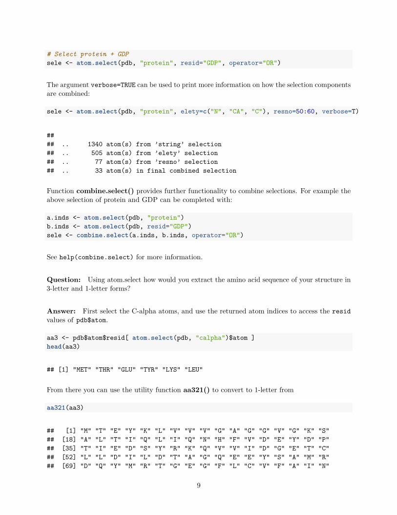
# Select protein + GDPsele <- atom.select(pdb, "protein", resid="GDP", operator="OR")

The argument verbose=TRUE can be used to print more information on how the selection componentsare combined:

sele <- atom.select(pdb, "protein", elety=c("N", "CA", "C"), resno=50:60, verbose=T)

#### .. 1340 atom(s) from ’string’ selection## .. 505 atom(s) from ’elety’ selection## .. 77 atom(s) from ’resno’ selection## .. 33 atom(s) in final combined selection

Function combine.select() provides further functionality to combine selections. For example theabove selection of protein and GDP can be completed with:

a.inds <- atom.select(pdb, "protein")b.inds <- atom.select(pdb, resid="GDP")sele <- combine.select(a.inds, b.inds, operator="OR")

See help(combine.select) for more information.

Question: Using atom.select how would you extract the amino acid sequence of your structure in3-letter and 1-letter forms?

Answer: First select the C-alpha atoms, and use the returned atom indices to access the residvalues of pdb$atom.

aa3 <- pdb$atom$resid[ atom.select(pdb, "calpha")$atom ]head(aa3)

## [1] "MET" "THR" "GLU" "TYR" "LYS" "LEU"

From there you can use the utility function aa321() to convert to 1-letter from

aa321(aa3)

## [1] "M" "T" "E" "Y" "K" "L" "V" "V" "V" "G" "A" "G" "G" "V" "G" "K" "S"## [18] "A" "L" "T" "I" "Q" "L" "I" "Q" "N" "H" "F" "V" "D" "E" "Y" "D" "P"## [35] "T" "I" "E" "D" "S" "Y" "R" "K" "Q" "V" "V" "I" "D" "G" "E" "T" "C"## [52] "L" "L" "D" "I" "L" "D" "T" "A" "G" "Q" "E" "E" "Y" "S" "A" "M" "R"## [69] "D" "Q" "Y" "M" "R" "T" "G" "E" "G" "F" "L" "C" "V" "F" "A" "I" "N"

9

## [86] "N" "T" "K" "S" "F" "E" "D" "I" "H" "Q" "Y" "R" "E" "Q" "I" "K" "R"## [103] "V" "K" "D" "S" "D" "D" "V" "P" "M" "V" "L" "V" "G" "N" "K" "C" "D"## [120] "L" "A" "A" "R" "T" "V" "E" "S" "R" "Q" "A" "Q" "D" "L" "A" "R" "S"## [137] "Y" "G" "I" "P" "Y" "I" "E" "T" "S" "A" "K" "T" "R" "Q" "G" "V" "E"## [154] "D" "A" "F" "Y" "T" "L" "V" "R" "E" "I" "R" "Q" "H" "K" "L"

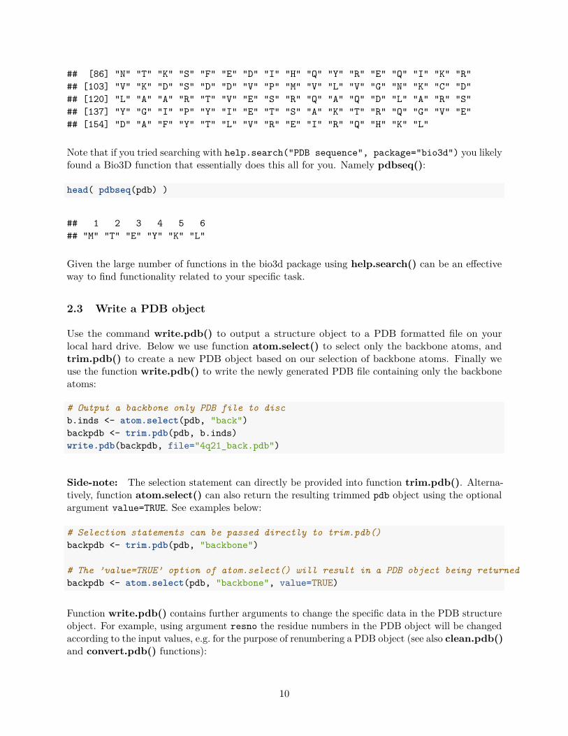
Note that if you tried searching with help.search("PDB sequence", package="bio3d") you likelyfound a Bio3D function that essentially does this all for you. Namely pdbseq():

head( pdbseq(pdb) )

## 1 2 3 4 5 6## "M" "T" "E" "Y" "K" "L"

Given the large number of functions in the bio3d package using help.search() can be an effectiveway to find functionality related to your specific task.

2.3 Write a PDB object

Use the command write.pdb() to output a structure object to a PDB formatted file on yourlocal hard drive. Below we use function atom.select() to select only the backbone atoms, andtrim.pdb() to create a new PDB object based on our selection of backbone atoms. Finally weuse the function write.pdb() to write the newly generated PDB file containing only the backboneatoms:

# Output a backbone only PDB file to discb.inds <- atom.select(pdb, "back")backpdb <- trim.pdb(pdb, b.inds)write.pdb(backpdb, file="4q21_back.pdb")

Side-note: The selection statement can directly be provided into function trim.pdb(). Alterna-tively, function atom.select() can also return the resulting trimmed pdb object using the optionalargument value=TRUE. See examples below:

# Selection statements can be passed directly to trim.pdb()backpdb <- trim.pdb(pdb, "backbone")

# The ’value=TRUE’ option of atom.select() will result in a PDB object being returnedbackpdb <- atom.select(pdb, "backbone", value=TRUE)

Function write.pdb() contains further arguments to change the specific data in the PDB structureobject. For example, using argument resno the residue numbers in the PDB object will be changedaccording to the input values, e.g. for the purpose of renumbering a PDB object (see also clean.pdb()and convert.pdb() functions):

10

# Renumber all residueswrite.pdb(backpdb, resno=backpdb$atom$resno+10)

# Assign chain B to all residueswrite.pdb(backpdb, chain="B")

2.4 Manipulate a PDB object

Basic functions for concatenating, trimming, splitting, converting, rotating, translating and super-posing PDB files are available but often you will want to manipulate PDB objects in a customway.

Below we provide a basic example of such a manipulation process where we read in a multi-chainedPDB structure, reassign chain identifiers, and renumber selected residues.

pdb <- read.pdb("4lhy")

# select chains A, E and Finds <- atom.select(pdb, chain=c("A", "E", "F"))

# trim PDB to selectionpdb2 <- trim.pdb(pdb, inds)

# assign new chain identifierspdb2$atom$chain[ pdb2$atom$chain=="E" ] <- "B"pdb2$atom$chain[ pdb2$atom$chain=="F" ] <- "C"

# re-number chain B and Cpdb2$atom$resno[ pdb2$atom$chain=="B" ] <- pdb2$atom$resno[ pdb2$atom$chain=="B" ] - 156pdb2$atom$resno[ pdb2$atom$chain=="C" ] <- pdb2$atom$resno[ pdb2$atom$chain=="C" ] - 156

# assign the GDP residue a residue number of 500pdb2$atom$resno[ pdb2$atom$resid=="GDP" ] <- 500

# use chain D for the GDP residuepdb2$atom$chain[ pdb2$atom$resid=="GDP" ] <- "D"

# Center, to the coordinate origin, and orient, by principal axes,# the coordinates of a given PDB structure or xyz vector.xyz <- orient.pdb(pdb2)

# write the new pdb object to filewrite.pdb(pdb2, xyz=xyz, file="4LHY_AEF-oriented.pdb")

11

2.5 Concatenate multiple PDBs

Function cat.pdb() can be used to concatenate two or more PDB files. This function containsmoreover arguments to re-assign residue numbers and chain identifiers. In the example below weillustrate how to concatenate 4q21 with specific components of 4lhy into a new PDB object:

# read two G-protein structuresa <- read.pdb("4q21")b <- read.pdb("4lhy")

a1 <- trim.pdb(a, chain="A")

b1 <- trim.pdb(b, chain="A")b2 <- trim.pdb(b, chain="E")b3 <- trim.pdb(b, chain="F")

# concatenate PDBsnew <- cat.pdb(a1, b1, b2, b3, rechain=TRUE)unique(new$atom$chain)

# write new PDB object to filewrite.pdb(new, file="4Q21-4LHY.pdb")

2.6 Coordinate superposition and structural alignment

Structure superposition is often essential for the direct comparison of multiple structures. Bio3Doffers versatile functionality for coordinate superposition at various levels. The simplest level issequence only based superposition:

# Align and superpose two or more structurespdbs <- pdbaln(c("4q21", "521p"), fit=TRUE)

Here the returned object is of class pdbs, which we will discuss in detail further below. For nownote that it contains a xyz numeric matrix of aligned C-alpha coordinates.

pdbs

## 1 . . . . 50## [Truncated_Name:1]4q21.pdb MTEYKLVVVGAGGVGKSALTIQLIQNHFVDEYDPTIEDSYRKQVVIDGET## [Truncated_Name:2]521p.pdb MTEYKLVVVGAVGVGKSALTIQLIQNHFVDEYDPTIEDSYRKQVVIDGET## *********** **************************************## 1 . . . . 50#### 51 . . . . 100## [Truncated_Name:1]4q21.pdb CLLDILDTAGQEEYSAMRDQYMRTGEGFLCVFAINNTKSFEDIHQYREQI## [Truncated_Name:2]521p.pdb CLLDILDTTGQEEYSAMRDQYMRTGEGFLCVFAINNTKSFEDIHQYREQI

12

## ******** *****************************************## 51 . . . . 100#### 101 . . . . 150## [Truncated_Name:1]4q21.pdb KRVKDSDDVPMVLVGNKCDLAARTVESRQAQDLARSYGIPYIETSAKTRQ## [Truncated_Name:2]521p.pdb KRVKDSDDVPMVLVGNKCDLAARTVESRQAQDLARSYGIPYIETSAKTRQ## **************************************************## 101 . . . . 150#### 151 . 168## [Truncated_Name:1]4q21.pdb GVEDAFYTLVREIRQHKL## [Truncated_Name:2]521p.pdb GVEDAFYTLVREIRQH--## ****************## 151 . 168#### Call:## pdbaln(files = c("4q21", "521p"), fit = TRUE)#### Class:## pdbs, fasta#### Alignment dimensions:## 2 sequence rows; 168 position columns (166 non-gap, 2 gap)#### + attr: xyz, resno, b, chain, id, ali, resid, sse, call

Underlying the pdbfit() function are calls to the seqaln() and fit.xyz() functions. The later oftheses does the actual superposition based on all the aligned positions returned from seqaln().Hence the superposition is said to be sequence based.

An alternative approach is to use a structure only alignment method (e.g. the mustang() function)as a basis for superposition. This is particularly useful when the structures (and hence usuallythe sequences) to be compared are dissimilar to the point where sequence comparison may giveerroneous results.

Variations of both these approaches are also implemented in Bio3D. For example, the functionstruct.aln() performs cycles of refinement steps of the alignment to improve the fit by removingatoms with a high structural deviation.

Note: The seqaln() function requires MUSCLE The MUSCLE multiple sequence alignmentprogram (available from the muscle home page) must be installed on your system and in the searchpath for executables in order to run functions pdbfit() and struct.aln() as these call the seqaln()function, which is based on MUSCLE. Please see the installation vignette for further details.

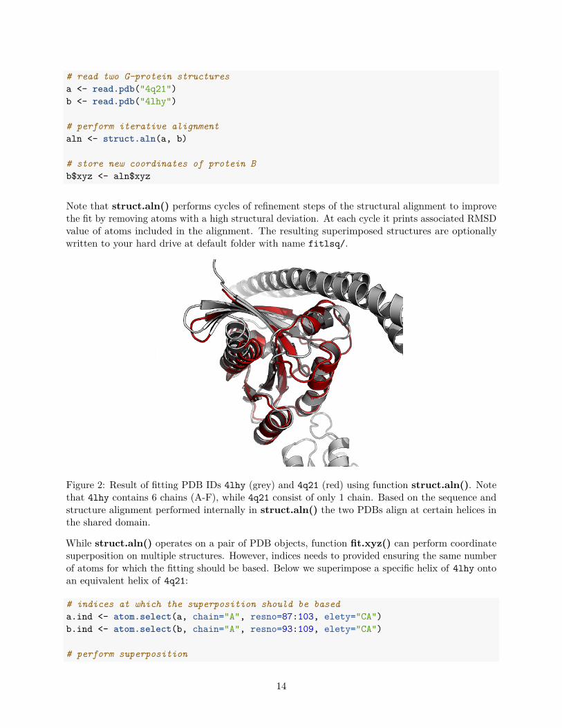
Function struct.aln() performs a sequence alignment followed by a structural alignment of twoPDB objects. This facilitates rapid superposition of two PDB structures with unequal, but relatedPDB sequences. Below we use struct.aln() to superimpose the multi-chained PDB ID 4lhy toPDB ID 4q21:

13

# read two G-protein structuresa <- read.pdb("4q21")b <- read.pdb("4lhy")

# perform iterative alignmentaln <- struct.aln(a, b)

# store new coordinates of protein Bb$xyz <- aln$xyz

Note that struct.aln() performs cycles of refinement steps of the structural alignment to improvethe fit by removing atoms with a high structural deviation. At each cycle it prints associated RMSDvalue of atoms included in the alignment. The resulting superimposed structures are optionallywritten to your hard drive at default folder with name fitlsq/.

Figure 2: Result of fitting PDB IDs 4lhy (grey) and 4q21 (red) using function struct.aln(). Notethat 4lhy contains 6 chains (A-F), while 4q21 consist of only 1 chain. Based on the sequence andstructure alignment performed internally in struct.aln() the two PDBs align at certain helices inthe shared domain.

While struct.aln() operates on a pair of PDB objects, function fit.xyz() can perform coordinatesuperposition on multiple structures. However, indices needs to provided ensuring the same numberof atoms for which the fitting should be based. Below we superimpose a specific helix of 4lhy ontoan equivalent helix of 4q21:

# indices at which the superposition should be baseda.ind <- atom.select(a, chain="A", resno=87:103, elety="CA")b.ind <- atom.select(b, chain="A", resno=93:109, elety="CA")

# perform superposition

14

xyz <- fit.xyz(fixed=a$xyz, mobile=b$xyz,fixed.inds=a.ind$xyz,mobile.inds=b.ind$xyz)

# write coordinates to filewrite.pdb(b, xyz=xyz, file="4LHY-at-4Q21.pdb")

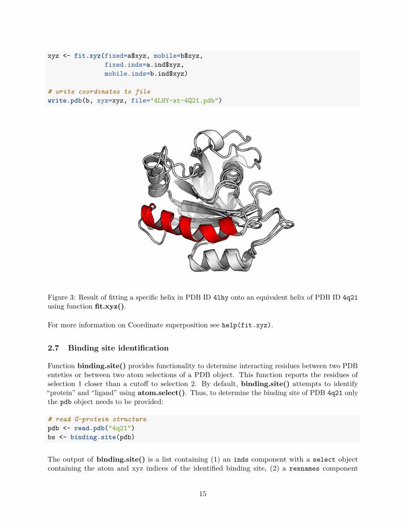
Figure 3: Result of fitting a specific helix in PDB ID 4lhy onto an equivalent helix of PDB ID 4q21using function fit.xyz().

For more information on Coordinate superposition see help(fit.xyz).

2.7 Binding site identification

Function binding.site() provides functionality to determine interacting residues between two PDBenteties or between two atom selections of a PDB object. This function reports the residues ofselection 1 closer than a cutoff to selection 2. By default, binding.site() attempts to identify“protein” and “ligand” using atom.select(). Thus, to determine the binding site of PDB 4q21 onlythe pdb object needs to be provided:

# read G-protein structurepdb <- read.pdb("4q21")bs <- binding.site(pdb)

The output of binding.site() is a list containing (1) an inds component with a select objectcontaining the atom and xyz indices of the identified binding site, (2) a resnames component

15

containing formatted residue names of the binding site residues, (3) resno and chain componentswith residue numbers and chain identifiers for the binding site residues.

# residue names of identified binding siteprint(bs$resnames)

## [1] "ALA-11 (A)" "GLY-12 (A)" "GLY-13 (A)" "VAL-14 (A)" "GLY-15 (A)"## [6] "LYS-16 (A)" "SER-17 (A)" "ALA-18 (A)" "PHE-28 (A)" "VAL-29 (A)"## [11] "ASP-30 (A)" "GLU-31 (A)" "TYR-32 (A)" "ASP-33 (A)" "PRO-34 (A)"## [16] "ILE-36 (A)" "ASP-57 (A)" "THR-58 (A)" "ALA-59 (A)" "ASN-116 (A)"## [21] "LYS-117 (A)" "ASP-119 (A)" "LEU-120 (A)" "THR-144 (A)" "SER-145 (A)"## [26] "ALA-146 (A)" "LYS-147 (A)"

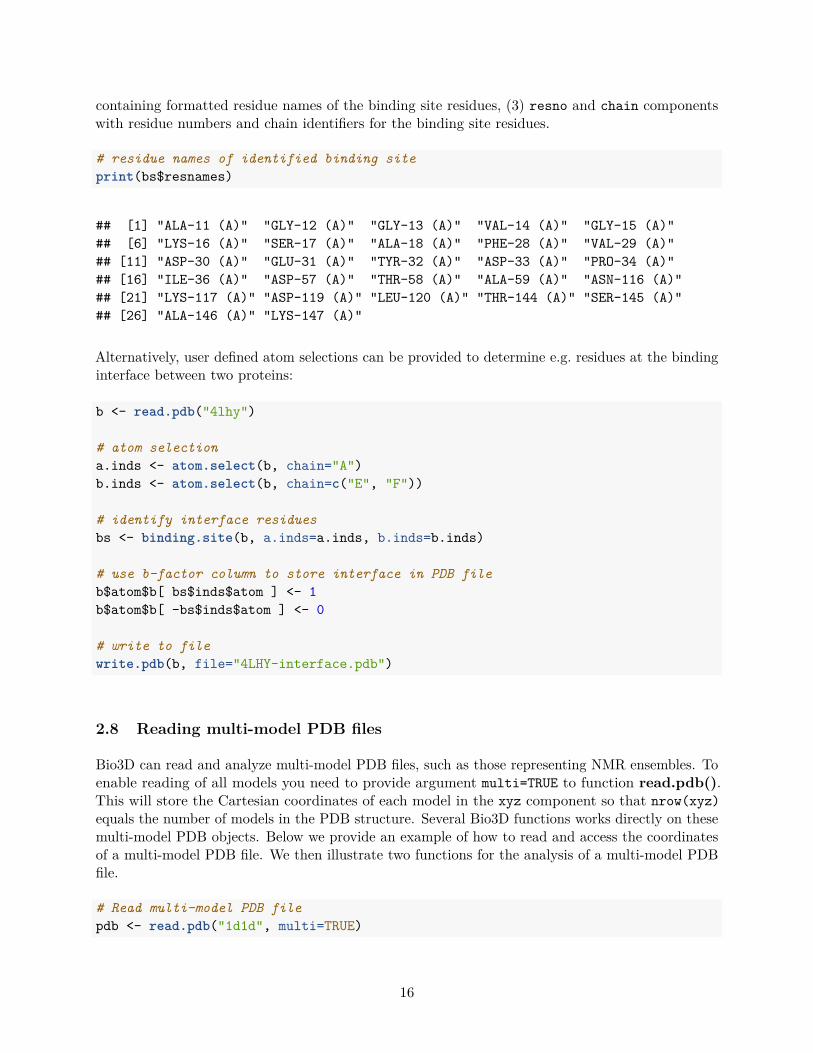
Alternatively, user defined atom selections can be provided to determine e.g. residues at the bindinginterface between two proteins:

b <- read.pdb("4lhy")

# atom selectiona.inds <- atom.select(b, chain="A")b.inds <- atom.select(b, chain=c("E", "F"))

# identify interface residuesbs <- binding.site(b, a.inds=a.inds, b.inds=b.inds)

# use b-factor column to store interface in PDB fileb$atom$b[ bs$inds$atom ] <- 1b$atom$b[ -bs$inds$atom ] <- 0

# write to filewrite.pdb(b, file="4LHY-interface.pdb")

2.8 Reading multi-model PDB files

Bio3D can read and analyze multi-model PDB files, such as those representing NMR ensembles. Toenable reading of all models you need to provide argument multi=TRUE to function read.pdb().This will store the Cartesian coordinates of each model in the xyz component so that nrow(xyz)equals the number of models in the PDB structure. Several Bio3D functions works directly on thesemulti-model PDB objects. Below we provide an example of how to read and access the coordinatesof a multi-model PDB file. We then illustrate two functions for the analysis of a multi-model PDBfile.

# Read multi-model PDB filepdb <- read.pdb("1d1d", multi=TRUE)

16

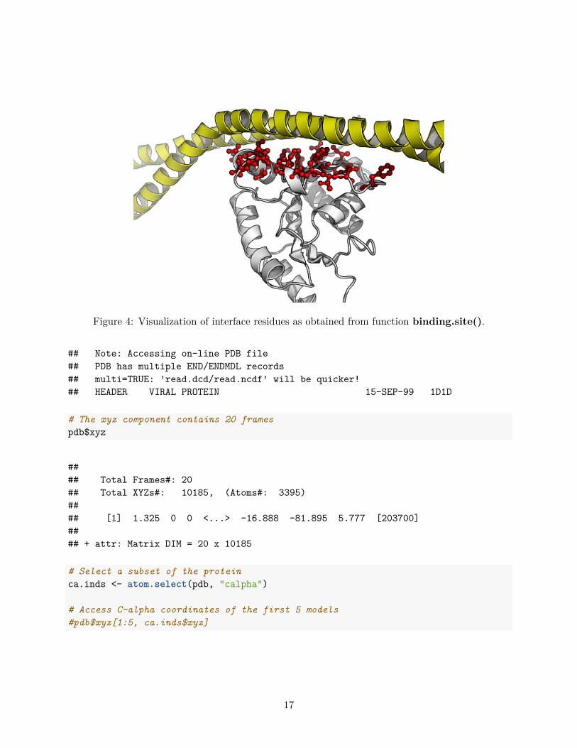
Figure 4: Visualization of interface residues as obtained from function binding.site().

## Note: Accessing on-line PDB file## PDB has multiple END/ENDMDL records## multi=TRUE: ’read.dcd/read.ncdf’ will be quicker!## HEADER VIRAL PROTEIN 15-SEP-99 1D1D

# The xyz component contains 20 framespdb$xyz

#### Total Frames#: 20## Total XYZs#: 10185, (Atoms#: 3395)#### [1] 1.325 0 0 <...> -16.888 -81.895 5.777 [203700]#### + attr: Matrix DIM = 20 x 10185

# Select a subset of the proteinca.inds <- atom.select(pdb, "calpha")

# Access C-alpha coordinates of the first 5 models#pdb$xyz[1:5, ca.inds$xyz]

17

2.9 Identification of dynamic domains

Function geostas() attempts to identify rigid domains in a protein (or nucleic acid) structurebased on knoweledge of its structural ensemble (as obtained a from multi-model PDB input file, anensemble of multiple PDB files (see section below), NMA or MD results). Below we demonstrate theidentification of such dynamic domains in a multi-model PDB and use function fit.xyz() to fit allmodels to one of the identified domains. We then use write.pdb() to store the aligned structuresfor further visualization, e.g. in VMD:

# Domain analysisgs <- geostas(pdb)

## .. 220 ’calpha’ atoms selected## .. ’xyz’ coordinate data with 20 frames## .. ’fit=TRUE’: running function ’core.find’## .. coordinates are superimposed to core region## .. calculating atomic movement similarity matrix (’amsm.xyz()’)## .. dimensions of AMSM are 220x220## .. clustering AMSM using ’kmeans’## .. converting indices to match input ’pdb’ object## (additional attribute ’atomgrps’ generated)

# Fit all frames to the ’first’ domaindomain.inds <- gs$inds[[1]]

xyz <- pdbfit(pdb, inds=domain.inds)

# write fitted coordinateswrite.pdb(pdb, xyz=xyz, chain=gs$atomgrps, file="1d1d_fit-domain1.pdb")

# plot geostas resultsplot(gs, contour=FALSE)

2.10 Invariant core identification

Function core.find() also works on a multi-model PDB file (or pdbs object, see below) to determinethe most invariant region a protein ensemble. Below we fit the NMR ensemble to the region identifiedby core.find():

# Invariant corecore <- core.find(pdb)

# fit to core regionxyz <- pdbfit(pdb, inds=core)

# write fitted coordinateswrite.pdb(pdb, xyz=xyz, file="1d1d_fit-core.pdb")

18

AMSM with Domain Assignment

Residue No.

Res

idue

No.

50

100

150

200

50 100 150 200

0.0

0.2

0.4

0.6

0.8

1.0

Figure 5: Plot of atomic movement similarity matrix with domain annotation for PDB ID 1d1d

19

Figure 6: Multi-model PDB with 20 frames superimposed on ‘domain 1’ (colored grey) identifiedusing function geostas(). See also related function core.find().

20

3 Constructing biological units

PDB crystal structure files typically detail the atomic coordinates for the contents of just onecrystal asymmetric unit. This may or may not be the same as the biologically-relevant assembly orbiological unit. For example, the PDB entry ‘2DN1’ of human hemoglobin stores one pair of alphaand beta globin subunits (see Figure 7). However, under physiological conditions the biologicalunit is known to be a tetramer (composed of two alpha and two beta subunits). In this particularcase, the crystal asymmetric unit is part of the biological unit. More generally, the asymmetricunit stored in a PDB file can be: (i) One biological unit; (ii) A portion of a biological unit, or (iii)Multiple biological units.

Figure 7: The alpha/beta dimer of human hemoglobin as stored in the PDB entry ‘2DN1’.

Reconstruction of the biological unit for a given PDB file can thus be essential for understandingstructure-function relationships. PDB files often provide information about how to constructbiological units via symmetry operations (i.e. rotation and translation) performed on the storedcoordinates. In Bio3D, the function read.pdb() automatically stores this information if available.The function biounit() can then be called to build biological units based on this informationstored within an appropriate ‘pdb’ object. The following example illustrates the construction of thehemoglobin tetramer from the dimer in the asymmetric unit of ‘2DN1’.

# Read PDB from online databasepdb <- read.pdb("2dn1")

## Note: Accessing on-line PDB file## HEADER OXYGEN STORAGE/TRANSPORT 25-APR-06 2DN1

21

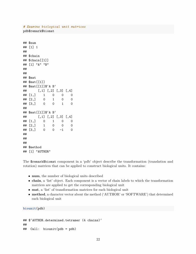
# Examine biological unit matricespdb$remark$biomat

## $num## [1] 1#### $chain## $chain[[1]]## [1] "A" "B"###### $mat## $mat[[1]]## $mat[[1]]$‘A B‘## [,1] [,2] [,3] [,4]## [1,] 1 0 0 0## [2,] 0 1 0 0## [3,] 0 0 1 0#### $mat[[1]]$‘A B‘## [,1] [,2] [,3] [,4]## [1,] 0 1 0 0## [2,] 1 0 0 0## [3,] 0 0 -1 0######## $method## [1] "AUTHOR"

The $remark$biomat component in a ‘pdb’ object describe the transformation (translation androtation) matrices that can be applied to construct biological units. It contains:

• num, the number of biological units described• chain, a ‘list’ object. Each component is a vector of chain labels to which the transformation

matrices are applied to get the corresponding biological unit• mat, a ‘list’ of transformation matrices for each biological unit• method, a character vector about the method (‘AUTHOR’ or ‘SOFTWARE’) that determined

each biological unit

biounit(pdb)

## $‘AUTHOR.determined.tetramer (4 chains)‘#### Call: biounit(pdb = pdb)

22

#### Total Models#: 1## Total Atoms#: 5012, XYZs#: 15036 Chains#: 4 (values: A B C D)#### Protein Atoms#: 4344 (residues/Calpha atoms#: 570)## Nucleic acid Atoms#: 0 (residues/phosphate atoms#: 0)#### Non-protein/nucleic Atoms#: 668 (residues: 472)## Non-protein/nucleic resid values: [ HEM (4), HOH (460), MBN (4), OXY (4) ]#### Protein sequence:## LSPADKTNVKAAWGKVGAHAGEYGAEALERMFLSFPTTKTYFPHFDLSHGSAQVKGHGKK## VADALTNAVAHVDDMPNALSALSDLHAHKLRVDPVNFKLLSHCLLVTLAAHLPAEFTPAV## HASLDKFLASVSTVLTSKYRHLTPEEKSAVTALWGKVNVDEVGGEALGRLLVVYPWTQRF## FESFGDLSTPDAVMGNPKVKAHGKKVLGAFSDGLAHLDNLKGTFA...<cut>...HKYH#### + attr: atom, helix, sheet, seqres, xyz,## calpha, call, log

The function biounit() returns a ‘list’ object. Each component of the ‘list’ represents a possiblebiological unit stored as a ‘pdb’ object. In above example, two new chains (chain C and D) areconstructed from symmetry operations performed on the original chains (chain A and B) see Figure8.

Figure 8: The biological unit of human hemoglobin (tetramer) built from PDB entry ‘2DN1’.

Side-note: The biological unit described in a PDB file is not always unique. Distinct methods,e.g. based on expertise of authors of the crystallographic structure or calucaltion of software (See

23

here for more details), may determine different multimeric state. Also, as mentioned above, onecrystal asymmetric unit may contain multiple biological units. The function biounit() returns allthe possible biological units listed in the file (and that is why the return value is a ‘list’ insteadof a simple ‘pdb’ object). It is dependent on users which biological unit is finally adopted forfurther analysis. Check the ‘names’ attributes of the returned ‘list’ for the determination methodand multimeric state of each biological unit. For example, the PDB entry ‘1KJY’ describes threepossible biological units for the G protein alpha subunit bound with GDI inhibitor. The commonway is to select either one of the two dimers (they have slightly distinct conformation) instead ofthe software predicted tetramer.

pdb <- read.pdb("1kjy")

## Note: Accessing on-line PDB file## HEADER SIGNALING PROTEIN 05-DEC-01 1KJY

bio <- biounit(pdb)names(bio)

## [1] "AUTHOR.determined.dimer (2 chains)"## [2] "AUTHOR.determined.dimer (2 chains)"## [3] "SOFTWARE.determined.tetramer (4 chains)"

Optionally, biounit() returns the biological unit as a multi-model ‘pdb’ object. In this case, thetopology of the ‘pdb’ (e.g. $atom) is the same as input, whereas additional coordinates generatedvia the symmetry operations are stored in distinc rows of $xyz. This is obtained by setting theargument multi=TRUE. It is particular useful for speed enhancements with biological units containingmany symmetric copies, for example a virus capsid:

pdb <- read.pdb("2bfu")

## Note: Accessing on-line PDB file## HEADER VIRUS 13-DEC-04 2BFU

bio <- biounit(pdb, multi = TRUE)bio

## $‘SOFTWARE.determined.multimer (120 chains)‘#### Call: biounit(pdb = pdb, multi = TRUE)#### Total Models#: 60## Total Atoms#: 5282, XYZs#: 950760 Chains#: 2 (values: L S)#### Protein Atoms#: 5282 (residues/Calpha atoms#: 558)## Nucleic acid Atoms#: 0 (residues/phosphate atoms#: 0)

24

#### Non-protein/nucleic Atoms#: 0 (residues: 0)## Non-protein/nucleic resid values: [ none ]#### Protein sequence:## MEQNLFALSLDDTSSVRGSLLDTKFAQTRVLLSKAMAGGDVLLDEYLYDVVNGQDFRATV## AFLRTHVITGKIKVTATTNISDNSGCCLMLAINSGVRGKYSTDVYTICSQDSMTWNPGCK## KNFSFTFNPNPCGDSWSAEMISRSRVRMTVICVSGWTLSPTTDVIAKLDWSIVNEKCEPT## IYHLADCQNWLPLNRWMGKLTFPQGVTSEVRRMPLSIGGGAGATQ...<cut>...TPPL#### + attr: atom, helix, sheet, seqres, xyz,## calpha, call

bio[[1]]$xyz

#### Total Frames#: 60## Total XYZs#: 15846, (Atoms#: 5282)#### [1] 21.615 -8.176 108.9 <...> -109.546 -20.972 -91.006 [950760]#### + attr: Matrix DIM = 60 x 15846

4 Working with multiple PDB files

The Bio3D package was designed to specifically facilitate the analysis of multiple structures fromboth experiment and simulation. The challenge of working with these structures is that they areusually different in their composition (i.e. contain differing number of atoms, sequences, chains,ligands, structures, conformations etc. even for the same protein as we will see below) and it isthese differences that are frequently of most interest.

For this reason Bio3D contains extensive utilities to enable the reading, writing, manipulation andanalysis of such heterogenous structure sets. This topic is detailed extensively in the separatePrincipal Component Analysis vignette available from http://thegrantlab.org/bio3d/tutorials.

Before delving into more advanced analysis (detailed in additional vignettes) lets examine how wecan read multiple PDB structures from the RCSB PDB for a particular protein and perform somebasic analysis:

# Download some example PDB filesids <- c("1TND_B","1AGR_A","1FQJ_A","1TAG_A","1GG2_A","1KJY_A")raw.files <- get.pdb(ids)

The get.pdb() function will download the requested files, below we extract the particular chainswe are most interested in with the function pdbsplit() (note these ids could come from the resultsof a blast.pdb() search as described in other vignettes). The requested chains are then alignedand their structural data stored in a new object pdbs that can be used for further analysis andmanipulation.

25

# Extract and align the chains we are interested infiles <- pdbsplit(raw.files, ids)pdbs <- pdbaln(files)

Below we examine the sequence and structural similarity.

# Calculate sequence identitypdbs$id <- basename.pdb(pdbs$id)seqidentity(pdbs)

## 1TND_B 1AGR_A 1FQJ_A 1TAG_A 1GG2_A 1KJY_A## 1TND_B 1.000 0.693 0.914 1.000 0.690 0.696## 1AGR_A 0.693 1.000 0.779 0.694 0.997 0.994## 1FQJ_A 0.914 0.779 1.000 0.914 0.776 0.782## 1TAG_A 1.000 0.694 0.914 1.000 0.691 0.697## 1GG2_A 0.690 0.997 0.776 0.691 1.000 0.991## 1KJY_A 0.696 0.994 0.782 0.697 0.991 1.000

## Calculate RMSDrmsd(pdbs, fit=TRUE)

## Warning in rmsd(pdbs, fit = TRUE): No indices provided, using the 313 non NA positions

## [,1] [,2] [,3] [,4] [,5] [,6]## [1,] 0.000 0.965 0.609 1.283 1.612 2.100## [2,] 0.965 0.000 0.873 1.575 1.777 1.914## [3,] 0.609 0.873 0.000 1.265 1.737 2.042## [4,] 1.283 1.575 1.265 0.000 1.687 1.841## [5,] 1.612 1.777 1.737 1.687 0.000 1.879## [6,] 2.100 1.914 2.042 1.841 1.879 0.000

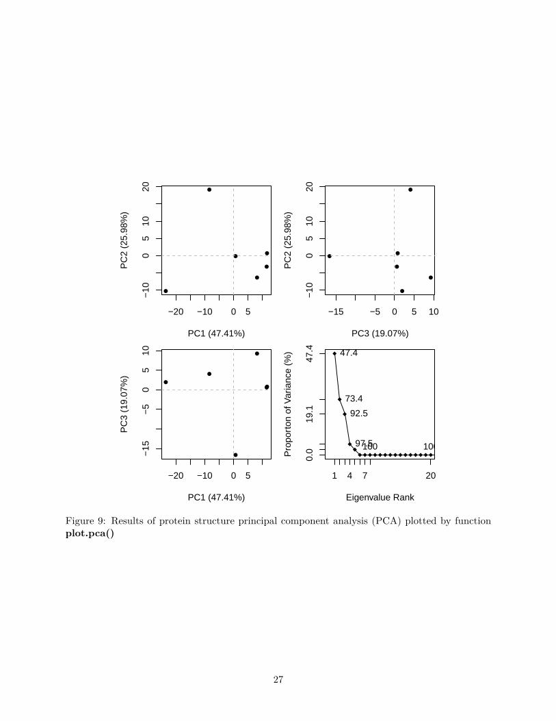
## Quick PCA (see Figure 9)pc <- pca(pdbfit(pdbs), rm.gaps=TRUE)plot(pc)

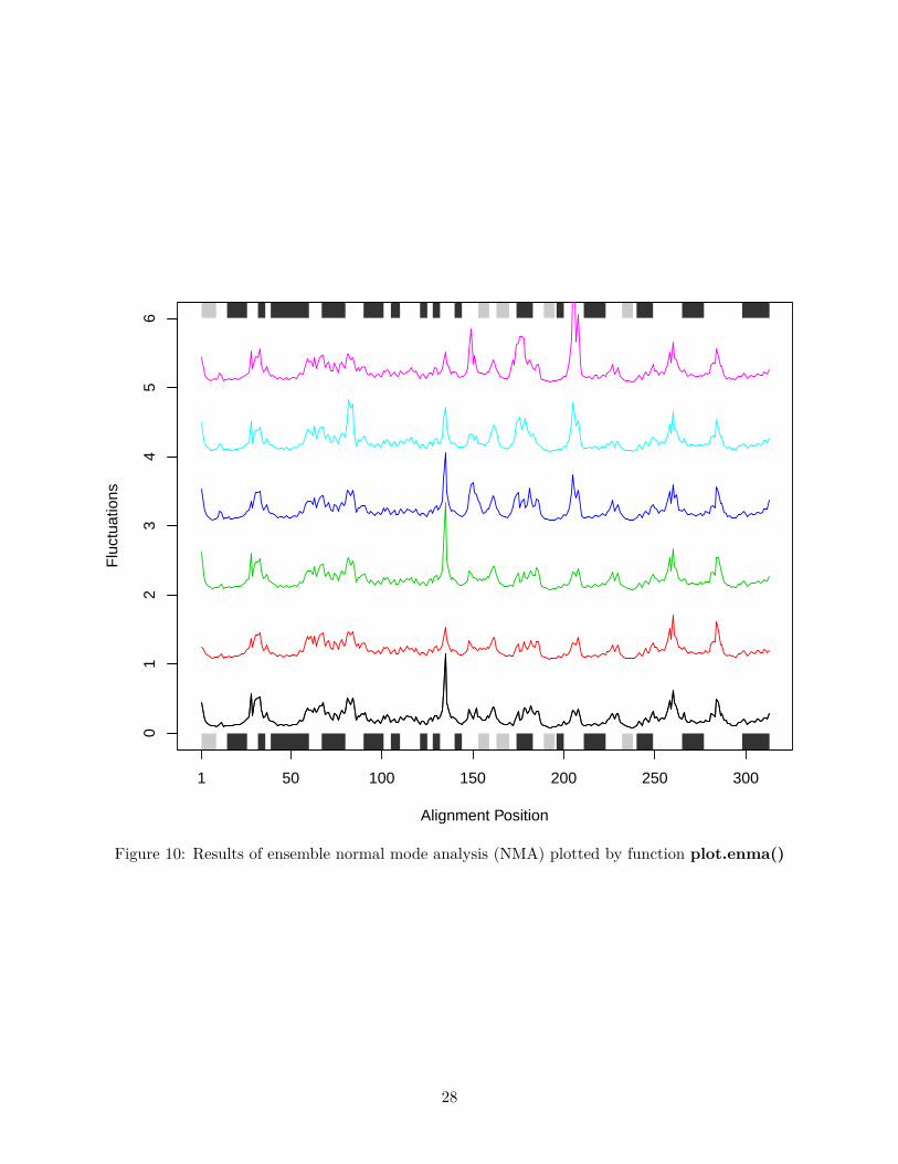
## Quick NMA of all structures (see Figure 10)modes <- nma(pdbs)plot(modes, pdbs, spread=TRUE)

Question: What effect does setting the fit=TRUE option have in the RMSD calculation? Whatwould the results indicate if you set fit=FALSE or disparaged this option? HINT: Bio3D functionshave various default options that will be used if the option is not explicitly specified by the user, seehelp(rmsd) for an example and note that the input options with an equals sign (e.g. fit=FALSE)have default values.

26

−20 −10 0 5

−10

05

1020

PC1 (47.41%)

PC

2 (2

5.98

%)

−15 −5 0 5 10−

100

510

20

PC3 (19.07%)

PC

2 (2

5.98

%)

−20 −10 0 5

−15

−5

05

10

PC1 (47.41%)

PC

3 (1

9.07

%)

1 4 7 20

0.0

19.1

47.4 47.4

73.4

92.5

97.5100 100

Eigenvalue Rank

Pro

port

on o

f Var

ianc

e (%

)

Figure 9: Results of protein structure principal component analysis (PCA) plotted by functionplot.pca()

27

01

23

45

6

1 50 100 150 200 250 300

Alignment Position

Flu

ctua

tions

Figure 10: Results of ensemble normal mode analysis (NMA) plotted by function plot.enma()

28

5 Where to next

If you have read this far, congratulations! We are ready to have some fun and move to other packagevignettes that describe more interesting analysis including advanced Comparative StructureAnalysis (where we will mine available experimental data and supplement it with simulation resultsto map the conformational dynamics and coupled motions of proteins), Trajectory Analysis(where we analyze molecular dynamics simulation trajectories), enhanced methods for NormalMode Analysis (where we will explore the dynamics of large protein families and superfamilies),and Correlation Network Analysis (where we will build and dissect dynamic networks formdifferent correlated motion data).

Document and current Bio3D session details

This document is shipped with the Bio3D package in both R and PDF formats. All code canbe extracted and automatically executed to generate Figures and/or the PDF with the followingcommands:

library(rmarkdown)render("Bio3D_pdb.Rmd", "all")

# Information about the current Bio3D sessionsessionInfo()

## R version 3.1.2 (2014-10-31)## Platform: x86_64-redhat-linux-gnu (64-bit)#### locale:## [1] LC_CTYPE=en_US.UTF-8 LC_NUMERIC=C## [3] LC_TIME=en_US.UTF-8 LC_COLLATE=en_US.UTF-8## [5] LC_MONETARY=en_US.UTF-8 LC_MESSAGES=en_US.UTF-8## [7] LC_PAPER=en_US.UTF-8 LC_NAME=C## [9] LC_ADDRESS=C LC_TELEPHONE=C## [11] LC_MEASUREMENT=en_US.UTF-8 LC_IDENTIFICATION=C#### attached base packages:## [1] stats graphics grDevices utils datasets methods base#### other attached packages:## [1] bio3d_2.2-0 rmarkdown_0.3.3#### loaded via a namespace (and not attached):## [1] digest_0.6.4 evaluate_0.5.5 formatR_1.0 grid_3.1.2## [5] htmltools_0.2.6 knitr_1.7 lattice_0.20-29 parallel_3.1.2## [9] stringr_0.6.2 tools_3.1.2 yaml_2.1.13

29

References

Grant, B.J., A.P.D.C Rodrigues, K.M. Elsawy, A.J. Mccammon, and L.S.D. Caves. 2006. “Bio3d:An R Package for the Comparative Analysis of Protein Structures.” Bioinformatics 22: 2695–96.doi:10.1093/bioinformatics/btl461.

Skjaerven, L., X.Q. Yao, G. Scarabelli, and B.J. Grant. 2015. “Integrating Protein StructuralDynamics and Evolutionary Analysis with Bio3D.” BMC Bioinformatics 15: 399. doi:10.1186/s12859-014-0399-6.

30