Behavioral Heterogeneity in Stock Prices

H. Peter Boswijk Cars H. Hommes Sebastiano Manzan

CeNDEF, University of Amsterdam, the Netherlands

Abstract

We estimate a dynamic asset pricing model characterized by heterogeneous boundedlyrational agents. The fundamental value of the risky asset is publicly available to allagents, but they have different beliefs about the persistence of deviations of stockprices from the fundamental benchmark. An evolutionary selection mechanism basedon relative past profits governs the dynamics of the fractions and switching of agentsbetween different beliefs or forecasting strategies. A strategy attracts more agents if itperformed relatively well in the recent past compared to other strategies. We estimatethe model to annual US stock price data from 1871 until 2003. The estimation resultssupport the existence of two expectation regimes. One regime can be characterizedas a fundamentalists regime, because agents believe in mean reversion of stock pricestoward the benchmark fundamental value. The second regime can be characterizedas a chartist, trend following regime because agents expect the deviations from thefundamental to trend. The fractions of agents using the fundamentalists and trendfollowing forecasting rules show substantial time variation and switching between pre-dictors. The model offers an explanation for the recent stock prices run-up. Before the90s the trend following regime was active only occasionally. However, in the late 90sthe trend following regime persisted and created an extraordinary deviation of stockprices from the fundamentals. Recently, the activation of the mean reversion regimehas contributed to drive stock prices back towards their fundamental valuation.

Acknowledgments. Earlier versions of this paper were presented at the IFAC symposium Com-putational Economics, Finance and Engineering, Seattle, June 28-30, 2003 and at seminars atTilburg University, the University of Amsterdam, the University of Udine and the University ofWarwick. Stimulating discussions and helpful comments are gratefully acknowledged. This re-search has been supported by the Netherlands Organization for Scientific Research (NWO) undera NWO-MaG Pionier grant.

Corresponding author: Sebastiano Manzan, Center for Nonlinear Dynamics in Economicsand Finance (CeNDEF), Department of Quantitative Economics, University of Amsterdam,Roetersstraat 11, NL-1018 WB Amsterdam, The Netherlands; e-mail: s.manzan@uva.nl, web-page: http://www.fee.uva.nl/cendef/.

Introduction

Historical evidence indicates that stock prices fluctuate heavily compared to indicators of

fundamental value. For example, the price to earnings ratio of the S&P500 was around 5

at the beginning of the 20s, but more than 25 about nine years later to fall back to about

5 again by 1933. In 1995 the price/earnings ratio of the S&P500 was close to 20, went up

to more than 40 at the beginning of 2000 and then quickly declined again to about 20 by

the end of 2003. Why do prices fluctuate so much compared to economic fundamentals?

This question has been heavily debated in financial economics. At the beginning

of the 80s, Shiller (1981) and LeRoy and Porter (1981) claimed that the stock market

exhibits excess volatility, that is, stock price fluctuations are significantly larger than

movements in underlying economic fundamentals. The debate evolved in two directions.

On the one hand, supporters of rational expectations and market efficiency proposed

modifications and extensions of the standard theory. In contrast, another part of the

literature focused on providing further empirical evidence against the efficiency of stock

prices and behavioral models to explain these phenomena. The debate has recently been

revived by the extraordinary surge of stock prices in the late 90s. The internet sector

was the main driving force behind the unprecedented increase in market valuations. Ofek

and Richardson (2002, 2003) estimated that in 1999 the average price-earnings ratio for

internet stocks was more than 600.

A recent overview of rational explanations based on economic fundamentals for the

increase in stock prices in the late 90s is e.g. given by Heaton and Lucas (1999). They

offer three reasons for the decrease of the equity premium, i.e. the difference between

expected returns on the market portfolio of risky stocks and riskless bonds. A first reason

is the observed increase of households’ participation in the stock market. This implies

spreading of equity risk among a larger population, which could explain a decrease of

the risk premium required by investors. Secondly, there is evidence that investors hold

more diversified portfolios compared to the past. In the 70s a large majority of investors

concentrated their equity holdings on one or two stocks. More recently households have

invested a large proportion of their wealth in mutual funds achieving a much better diver-

sification of risk. Both facts justify a decrease of the required risk premium by investors.

Although the wider participation seems unlikely to play an important role in the surge of

stock prices in the 90s, the increased portfolio diversification could at least partly account

for the decrease in the equity premium and the unprecedented increase in market valua-

tions. A third, fundamental explanation for the surge of the stock market that has been

proposed is a shift in corporate practice from paying dividends to repurchasing shares as

1

an alternative measure to distribute cash to shareholders. In this case dividends do not

measure appropriately the profitability of the asset and such a shift in corporate practice

explains, at least partly, an increase in price-earnings or price-dividend ratios or equiva-

lently a decrease of the risk premium. Further evidence on this issue is provided by Fama

and French (2001).

Some recent papers attempt a quantitative evaluation of the decrease in the equity

premium. Fama and French (2002) argue that, based on average dividend growth, the real

risk premium has significantly decreased from 4.17% in the period 1872-1950 to 2.5% after

1950. Jagannathan, McGrattan, and Scherbina (2000) go even further and, comparing

the equity yield to a long-term bonds yield, reach the conclusion that the risk premium

from 1970 onwards was approximately 0.7%. That is, investors require almost the same

return to invest in stocks and in 20 years government bonds. The explanations above

indicate structural, fundamental reasons for a long-horizon tendency of the risk premium

to decrease, or equivalently for an increase of the valuation of the aggregate stock market.

However, to quantify the decrease in the equity premium is difficult and the estimates

provided earlier are questionable. Although fundamental reasons may partly explain an

increase of stock prices, the dramatic movements e.g. in the nineties are hard to interpret

as an adjustment of stock prices toward a new fundamental value.

Another strand of recent literature has provided empirical evidence on market ineffi-

ciencies and proposed a behavioral explanation. Hirshleifer (2001) and Barberis and Thaler

(2003) contain extensive surveys of behavioral finance and empirical results both for the

cross-section of returns and for the aggregate stock market. Much attention has been

paid to the continuation of short-term returns and their reversal in the long-run. This

was documented both for the cross-section of returns by de Bondt and Thaler (1985),

and Jegadeesh and Titman (1993) and for the aggregate market by Cutler, Poterba, and

Summers (1991). At short run horizons of 6-12 months, past winners outperform past

losers, whereas at longer horizons of e.g. 3-5 years, past losers outperform past winners.

A behavioral explanation of this phenomenon is that at horizons from 3 months to a year,

investors underreact to news about fundamentals of a company or the economy. They

slowly adjust their valuations to incorporate the news and create positive serial correla-

tion in returns. However, in the adjustment process they drive prices too far from what is

warranted by the fundamental news. This shows up in returns as negative correlation at

longer horizons. Several behavioral models have been developed to explain the empirical

evidence. Barberis, Shleifer, and Vishny (1998), henceforth BSV, assume that agents are

affected by psychological biases in forming expectations about future cash flows. BSV

consider a model with a representative risk-neutral investor in which the true earnings

2

process is a random walk, but investors believe that earnings are generated by one of two

regimes, a mean-reverting regime and a trend regime. When confronted with positive fun-

damental news investors are too conservative in extrapolating the appropriate implication

for the immediate asset valuation. However, they overreact to a stream of positive funda-

mental news because they interpret it as representative of a new regime of higher growth.

The model is able to replicate the empirical observation of continuation and reversal of

stock returns. Another behavioral model that aims at explaining the same stylized facts is

Daniel, Hirshleifer, and Subrahmanyam (1998), henceforth DHS. Their model stresses the

importance of biases in the interpretation of private information. DHS assume that in-

vestors are overconfident and overestimate the precision of the private signal they receive

about the asset pay-off. The overconfidence increases if the private signal is confirmed

by public information, but decreases slowly if the private signal contrasts with public in-

formation. The model of BSV assumes that all information is public and that investors

misinterpret fundamental news. In contrast, DHS emphasize overconfidence concerning

private information compared to what is warranted by the public signal. These models

aim to explain the continuation and reversal in the cross-section of returns. However, as

suggested by Barberis and Thaler (2003), both models are also suitable to explain the

aggregate market dynamics.

In this paper we consider an asset pricing model with behavioral heterogeneity and

estimate the model using yearly S&P 500 data from 1871 to 2003. The model is a reformu-

lation, in terms of price-to-cash flow ratios, of the asset pricing model with heterogeneous

beliefs introduced by Brock and Hommes (1997, 1998). Agents are boundedly rational

and have heterogeneous beliefs about future pay-offs of a risky asset. Beliefs about fu-

ture cash flows are homogeneous and correct, but agents disagree on the speed the asset

price will mean-revert back towards its fundamental value. A key feature of the model

is the endogenous, evolutionary selection of beliefs or expectation rules based upon their

relative past performance, as proposed by Brock and Hommes (1997). The estimation of

our model on yearly S&P 500 data suggests that behavioral heterogeneity is significant

and that there are two different regimes, a “mean reversion” regime and a “trend fol-

lowing” regime. To each regime, there corresponds a different (class of) investor types:

fundamentalists and trend followers. These two investor types co-exist and their fractions

show considerable fluctuations over time. The mean-reversion regime corresponds to the

situation when the market is dominated by fundamentalists, who recognize a mispricing

of the asset and expect the stock price to move back towards its fundamental value. The

other trend following regime represents a situation when the market is dominated by trend

followers, expecting continuation of say good news in the (near) future and expect positive

3

stock returns. Before the 90s, the trend regime is activated only occasionally and never

persisted for more than two consecutive years. However, in the late 90s the fraction of

investors believing in a trend increased close to one and persisted for a number of years.

The prediction of an explosive growth of the stock market by trend followers was confirmed

by annual returns of more than 20% for four consecutive years. These high realized yearly

returns convinced many investors to also adopt the trend following belief thus reenforcing

an unprecedented deviation of stock prices from their fundamental value.

The outline of the paper is as follows. Section I discusses some closely related literature.

Section II describes the asset pricing model with heterogeneous beliefs and endogenous

switching, while Section III presents the estimation results. Section IV discusses empirical

implications of our model, in particular the impulse response to a permanent positive

shock to the fundamental and a simulation based prediction of how likely or unlikely high

valuation ratios are in the future. Finally, Section V concludes.

I Related Literature

Our model is closely related to other work in behavioral finance, and it is useful to discuss

some similarities and differences with other behavioral models in the recent literature. We

also refer the reader to the extensive surveys on behavioral finance by Barberis and Thaler

(2003) and Hirshleifer (2001) and the recent survey on dynamic heterogeneous agent mod-

els in economics and finance in Hommes (2005). Behavioral heterogeneity differentiates

our model from Barberis, Shleifer, and Vishny (1998) and Daniel, Hirshleifer, and Sub-

rahmanyam (1998) who both assume a representative agent. In contrast, we allow for the

coexistence of different types of investors with heterogeneous expectations about future

payoffs and evolutionary switching between different investment strategies. Disagreement

in asset pricing models can arise because of two assumptions: differential information and

differential interpretation. In the first case, there is an information asymmetry between

one group of agents that observes a private signal and the rest of the population that

has to learn the fundamental value from public information such as prices. Asymmetric

information causes heterogeneous expectations among agents. Recent models of this type

are Grundy and Kim (2002) and Biais and Bossaerts (2003). The second assumption is

based on the fact that a public signal can be interpreted in different ways by investors.

Agents use different ‘models of the market’ to update their subjective valuation based on

the earnings news and this might lead them to hold different beliefs. Empirical evidence

to support this hypothesis has been provided by Kandel and Pearson (1995) and Bam-

ber, Barron, and Stober (1999). They analyze the revisions of analysts earnings forecasts

4

around announcements. They provide significant evidence for the hypothesis that beliefs

among financial analysts are indeed heterogeneous. These findings are able to explain

the abnormal volume of trade around earnings announcements even when prices do not

change. However, the heterogeneity of expectations might play a significant role in asset

pricing. A large number of models have been proposed that incorporate this hypothesis.

A few relevant references are Harris and Raviv (1993) and Hong and Stein (1999). Some

papers have also suggested that the combination of differences in beliefs and short-sales

constraints can explain persistent deviations of stock prices from intrinsic valuations. In

the presence of short-sales constraints, investors that are pessimistic about a stock will not

be able to short the stock and they will simply not hold it. However, optimistic agents will

buy the stock and the market price will be such that it reflects only the optimistic valua-

tions in the population. This hypothesis was introduced by Miller (1977) and is recently

reconsidered by Chen, Hong, and Stein (2002) and Hong and Stein (2003). The empirical

implications for the cross-section of stock returns is investigated by Diether, Malloy, and

Scherbina (2002).

In our model we assume that the fundamental value of the asset is common knowledge.

However, investors have heterogeneous beliefs about the speed of reversion of stock prices

towards the intrinsic valuation. They expect that a mispricing will adjust at different

horizons. For example, assume the market is currently overvalued. In our setup, this

is common knowledge but one group of agents, the fundamentalists, is pessimistic and

believes that this situation will soon be corrected. However, the rest of the population, the

trend followers, is optimistic and believes that in the short run the price trend will continue.

Our model allows for the coexistence of groups with different sentiment about the evolution

of the stock market. This assumption is supported by the survey evidence in Shiller (2000),

Fisher and Statman (2002) and Vissing-Jorgensen (2003). These surveys involve both

institutional and individual investors from different sources during the 90s. A common

result emerges from them. During the surge in stock prices of the 90s, a large fraction

of investors were aware of the overvaluation but they continued to buy stocks because

they expected the mispricing to be corrected only at longer-horizons. Vissing-Jorgensen

(2003) reports that at the beginning of 2000, 50% of individual investors considered the

stock market to be overvalued, approximately 25% believed that it was fairly valued and

less than 10% that it was undervalued. This is a clear indication that opinions among

individual investors were heterogeneous and that they had different beliefs about the

prospect of the stock market. Similar survey evidence for exchange rate expectations

has been found by Frankel and Froot (1987, 1990). Their survey data analysis shows that

financial experts extrapolate past trends in exchange rates at short horizons from 1 week up

5

to 3 months, whereas the same experts have mean reverting expectations at longer horizons

of 6-12 months. They also provide evidence that from the end of the seventies until the

mid eighties the relative proportion among forecasting services of trend-following beliefs

compared to fundamental mean reverting rules, increased. They argue that the relative

popularity of technical trading rules compared to fundamental rules may have amplified

the strong rise of the dollar exchange rate in the early eighties and its subsequent fall

after February 1985. Shiller (2000) finds similar evidence that the sentiment of investors

varies significantly over time. Both for institutional and individual investors there is

evidence that they become more optimistic (or more bullish) in response to significant

increases in the recent performance of the stock market. This evidence supports one

of the key assumption of our model: evolutionary switching between different beliefs or

investment strategies. We assume that agents adopt a belief based on its past performance

relative to the competing strategies. If a belief performs relatively well, as measured by

realized profits, it attracts more investors. Instead, the fraction of the agents using the

“losing” strategies will decrease. Realized returns thus contribute to give more support

to some of the beliefs strategies rather than others and lead to time variation in the

sentiment of the market. The assumption of evolutionary switching among beliefs adds

a dynamical aspect that is missing in most of the models with heterogeneous opinions

mentioned above. In our model investors are boundedly rational because they learn from

the past performance of the strategies which one is more likely to be successful in the near

future. They do not use in every period the same predictor and make mistakes, but switch

between beliefs in order to minimize their errors. Our model is also consistent with asset

market laboratory experiments such as Smith, Suchanek, and Williams (1988), who found

bubbles and crashes in their asset market experiments. Recent asset pricing laboratory

experiments in Hommes, Sonnemans, Tuinstra, and van de Velden (2005) show that agents

may coordinate expectations on trend following behavior and mean reversion, leading to

asset price fluctuations around a constant fundamental price.

Our paper is also related to earlier work on assessing the contributions of market fun-

damentals and rational bubbles to stock-price fluctuations, for example in Blanchard and

Watson (1982), Flood and Hodrick (1990), West (1987) and Diba and Grossman (1988).

In our behavioral model agents are not fully rational, but at least boundedly rational in

the sense that they are driven by short run profitability. In particular, the model of Evans

(1991) of periodically collapsing rational bubbles is somewhat similar in spirit. In this

model asset prices grow at a rate larger than the risk free rate for some time, but have

an exogenously given positive probability of collapsing in each period. In our behavioral

model asset prices also exhibit different phases of larger growth than the discount rate,

6

when trend followers dominate the market, and mean reversion when fundamentalists dom-

inate, with the probability of switching between the two phases determined endogenously

by recent realized profits.

Our paper may be seen as one of the first attempts to estimate a behavioral model with

heterogeneous agents on stock market data. Only few attempts have been made to estimate

a heterogeneous agent model (HAM). An early example is Shiller (1984), who presents

a heterogeneous agent model with smart money traders, having rational expectations,

versus ordinary investors (whose behavior is in fact not modeled at all). Shiller estimates

the fraction of smart money investors over the period 1900-1983, and finds considerable

fluctuations of the fraction over a range between 0 and 50%. More recently, Baak (1999)

and Chavas (2000) estimate HAMs on hog and beef market data, and found evidence for

the heterogeneity of expectations. For the beef market Chavas (2000) finds that about

47% of the beef producers behave naively (using only the last price in their forecast),

18% of the beef producers behaves rationally, whereas 35% behaves quasi-rationally (i.e.

use a univariate autoregressive time series model of prices in forecasting). Winker and

Gilli (2001) and Gilli and Winker (2003) estimate the exchange rate model of Kirman

(1991, 1993) with fundamentalists and chartists, using the daily DM-US$ exchange rates

1991-2000. Their estimated parameter values correspond to a bimodal distribution of

agents, and Gilli and Winker (2003) conclude that the foreign exchange market can be

better characterized by switching moods of the investors than by assuming that the mix

of fundamentalists and chartists remains stable over time. Westerhoff and Reitz (2003)

also estimate an HAM with fundamentalists and chartists to exchange rates and find

considerable fluctuations of the market impact of fundamentalists. All these empirical

papers suggest that heterogeneity is important in explaining the data, but much more

work is needed to investigate the robustness of this empirical finding. Our paper may be

seen as one of the first attempts to estimate a behavioral HAM on stock market data and

investigate whether behavioral heterogeneity is significant.

II The Model

We consider the asset pricing model with heterogeneous beliefs introduced by Brock and

Hommes (1997, 1998) and reformulate the model in terms of price to cash flow in order to

estimate the model on yearly S&P 500 data. There are two assets available, a risky and a

riskless asset. The riskless asset is in perfectly elastic supply and pays a constant return

r. The risky asset is in zero net supply and pays an uncertain cash flow Yt in each period.

The price of the risky asset in period t is denoted by Pt. The excess return of the risky

7

asset is defined as

Rt+1 = Pt+1 + Yt+1 − (1 + r)Pt. (1)

We assume that investors have heterogeneous beliefs about future payoffs. In particular, we

assume that agents choose among H types of beliefs or forecasting rules. The expectation

of investors type h about the conditional mean and variance of the excess return are

Eh,t[Rt+1] and Vh,t[Rt+1], for h = 1, ..., H. We assume that type h agents have a myopic

mean-variance demand function with risk aversion parameter ah, given by

zh,t =Eh,t[Rt+1]

ahVh,t[Rt+1]. (2)

For analytical tractability, following Brock and Hommes (1998), we assume that all in-

vestors have the same risk aversion parameter, ah = a, and that they have homogeneous

expectations about the conditional variance, Vh,t[Rt+1] ≡ Vt[Rt+1]. The only source of

heterogeneity that we allow in the model concerns the beliefs about the future payoffs of

the risky asset. We denote the fraction of investors in the economy using predictor h at

time t by nh,t. Under the assumption of zero net supply of the risky asset, the market

clearing equation is

H∑

h=1

nh,tEh,t[Pt+1 + Yt+1] − (1 + r)Pt

aVt[Rt+1]= 0, (3)

and the equilibrium pricing equation is thus given by

Pt =1

1 + r

H∑

h=1

nh,tEh,t(Pt+1 + Yt+1). (4)

According to (4) the price at time t of the risky asset is given by the discounted, weighted

average (by the fractions) of investors’ beliefs about next period pay-offs. Notice that the

equilibrium pricing equation (4) is equivalent to

r =H∑

h=1

nh,tEh,t[Pt+1 + Yt+1 − Pt]

Pt, (5)

that is, in equilibrium the average required rate of return for investors to hold the risky

asset equals the discount rate r. In the estimation of the model in Section ?? the discount

rate r will be set equal to the sum of the (risk free) interest rate and the required risk

premium on stocks1. From (4) it is clear that the equilibrium price will be high if an

optimistic type dominates the market, that is, when the fraction of investors expecting

a high next period payoff is large. On the other hand, pessimistic beliefs about future

8

payoffs will drive the equilibrium price to lower levels. We assume that investors have

homogeneous expectations about the cash flow. In contrast to Brock and Hommes (1998),

who assume an IID process for the cash flow, we consider a non-stationary cash flow with

a constant growth rate. More precisely, we assume that log Yt is a Gaussian random walk

with drift, that is,

log Yt+1 = µ + log Yt + υt+1, υt+1 ∼ i.i.d. N(0, σ2υ), (6)

This impliesYt+1

Yt= eµ+υt+1 = eµ+ 1

2σ2

υeυt+1−1

2σ2

υ = (1 + g)εt+1, (7)

where g = eµ+ 1

2σ2

υ − 1 and εt+1 = eυt+1+ 1

2σ2

υ , which implies Et(εt+1) = 1. We assume that

all types have correct beliefs on the cash flow, that is,

Eh,t[Yt+1] = Et[Yt+1] = (1 + g)YtEt[εt+1] = (1 + g)Yt. (8)

Since the cash flow is an exogenously given stochastic process it seems natural to assume

that agents have learned the correct beliefs on next periods cash flow Yt+1. In particular,

boundedly rational agents can learn about the constant growth rate e.g. by running a

simple regression of Yt/Yt−1 on a constant. In contrast, prices are determined endogenously

and in particular prices are affected by expectations about next period’s price. In a

heterogeneous world, agreement about next period’s price therefore seems more unlikely

than agreement about the cash flow, and therefore we will assume heterogeneous beliefs

about next period’s price as discussed below. The pricing equation (4) can be reformulated

in terms of price-to-cash-flow (PY) ratio, δt = Pt/Yt, as

δt =1

R∗

{

1 +H∑

h=1

nh,tEh,t[δt+1]

}

, R∗ =1 + r

1 + g. (9)

where we assume that the dividend growth Yt+1/Yt is conditionally independent of δt+1,

that is,

Eh,t

[Pt+1

Yt

]= Eh,t[δt+1]Eh,t

[Yt+1

Yt

]= (1 + g)Eh,t[δt+1]. (10)

In the special case, when all agents have rational expectations the equilibrium pricing

equation (4) simplifies to

Pt =1

1 + rEt(Pt+1 + Yt+1). (11)

9

It is well known that, in the case of a constant growth rate g for dividends, the rational

expectations fundamental price, P ∗t , of the risky asset is given by

P ∗t =

1 + g

r − gYt, r > g, (12)

or equivalently, in terms of price-to-cash flow ratios

δ∗t =P ∗

t

Yt=

1 + g

r − g≡ m, (13)

We will refer to P ∗t as the fundamental price and to δ∗t as the fundamental PY-ratio.

When all agents are rational the pricing equation (9) in terms of the PY-ratio, δt = Pt/Yt,

becomes

δt =1

R∗{1 + Et[δt+1]} . (14)

In terms of the deviation from the fundamental ratio, xt = δt − δ∗t = δt −m, this simplifies

to

xt =1

R∗Et[xt+1]. (15)

Under heterogeneity in expectations, the pricing equation (9) is expressed in terms of xt

as

xt =1

R∗

H∑

h=1

nh,tEh,t[xt+1]. (16)

Heterogeneous beliefs

We now specify how agents form their beliefs about next period’s PY-ratio. We assume

that the fundamental PY-ratio is known to all investors. However, agents have different

beliefs about the persistence of the deviation from the fundamental. The expectation of

belief type h about next period PY-ratio is expressed as

Eh,t[δt+1] = Et[δ∗t+1] + fh(xt−1, ..., xt−L) = m + fh(xt−1, ..., xt−L), (17)

where δ∗t represents the fundamental PY-ratio, Et(δ∗t+1) = m is the rational expectation of

the PY-ratio available to all agents, xt is the deviation of the PY-ratio from its fundamental

value and fh(·) represents the expected transitory deviation of the PY-ratio from the

fundamental value, depending on L past deviations. The information available to investors

at time t includes present and past cash flows and past prices. In other words, we do not

allow agents to react to the contemporaneous equilibrium price but only to past realized

prices. This assumption about the information set available to traders was previously used

by Hellwig (1982) and Blume, Easley, and O’Hara (1994) in a rational expectations setup.

10

Another way of interpreting this assumption is that investors can only trade using market

orders. A similar assumption is also used by Hong and Stein (1999). At the beginning

of the period agents choose their optimal demand of the risky asset determined by past

realized prices and at the end of period t, the market clearing price Pt is determined. We

can reformulate Equation (17) in terms of deviations from the fundamental PY-ratio, xt,

as

Eh,t[xt+1] = fh(xt−1, ..., xt−L). (18)

The function f(·) can be interpreted as the belief of investors type h about the evolution

of the transitory component in the asset price. Note that the rational expectations, fun-

damental benchmark is nested in our heterogeneous agent model as a special case when

fh ≡ 0 for all types h. In Section ?? we will estimate the model to investigate whether

deviations from the benchmark fundamental are significant. We can now express Equa-

tion (9) in term of deviations of the PY-ratio from the fundamental valuation, xt, and

obtain the simpler form

R∗xt =H∑

h=1

nh,tfh(xt−1, ..., xt−L). (19)

From this equilibrium equation it is immediately clear that the adjustment towards the

fundamental PY-ratio will be slow if a majority of investors has persistent beliefs about

it.

Evolutionary selection of expectations

In addition to the evidence of persistent deviations from the fundamentals there is also

significant evidence of time variation in the sentiment of investors. This has been docu-

mented, for example, by Shiller (2000) using survey data. In the model considered here,

agents are boundedly rational and switch between different forecasting strategies accord-

ing to relative recently realized profits. At the beginning of period t the realized profits

for each of the strategies are publicly available. We denote by πh,t−1 the realized profits

of type h at the end of period t − 1, given by

πh,t−1 = Rt−1zh,t−2 = Rt−1Eh,t−2[Rt−1]

aVt−2[Rt−1], (20)

where Rt−1 = Pt−1+Yt−1−(1+r)Pt−2 is the realized excess return, as given in (1), at time

t − 1 and zh,t−2 indicates the demand of the risky asset by belief type h, as given in (2),

formed in period t − 2. In other words, πh,t−1 represents the excess profit realized in the

previous period by strategy h, in terms of quantities observed at the beginning of period t.

11

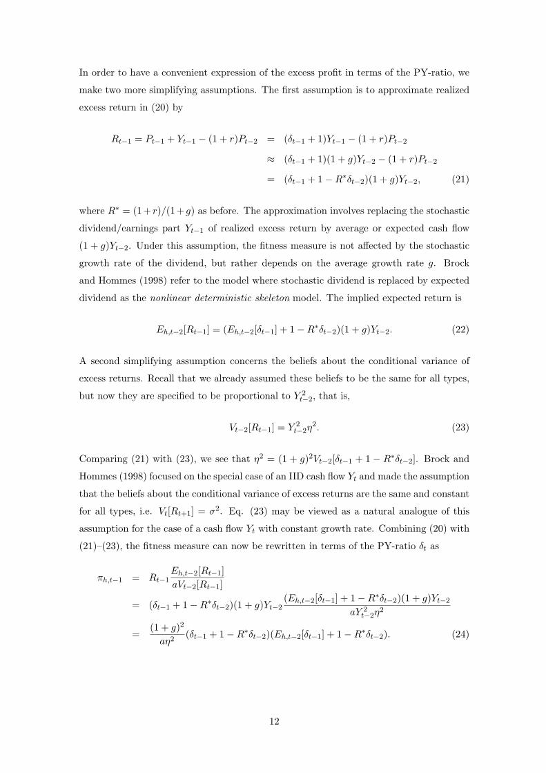
In order to have a convenient expression of the excess profit in terms of the PY-ratio, we

make two more simplifying assumptions. The first assumption is to approximate realized

excess return in (20) by

Rt−1 = Pt−1 + Yt−1 − (1 + r)Pt−2 = (δt−1 + 1)Yt−1 − (1 + r)Pt−2

≈ (δt−1 + 1)(1 + g)Yt−2 − (1 + r)Pt−2

= (δt−1 + 1 − R∗δt−2)(1 + g)Yt−2, (21)

where R∗ = (1+ r)/(1+g) as before. The approximation involves replacing the stochastic

dividend/earnings part Yt−1 of realized excess return by average or expected cash flow

(1 + g)Yt−2. Under this assumption, the fitness measure is not affected by the stochastic

growth rate of the dividend, but rather depends on the average growth rate g. Brock

and Hommes (1998) refer to the model where stochastic dividend is replaced by expected

dividend as the nonlinear deterministic skeleton model. The implied expected return is

Eh,t−2[Rt−1] = (Eh,t−2[δt−1] + 1 − R∗δt−2)(1 + g)Yt−2. (22)

A second simplifying assumption concerns the beliefs about the conditional variance of

excess returns. Recall that we already assumed these beliefs to be the same for all types,

but now they are specified to be proportional to Y 2t−2, that is,

Vt−2[Rt−1] = Y 2t−2η

2. (23)

Comparing (21) with (23), we see that η2 = (1 + g)2Vt−2[δt−1 + 1 − R∗δt−2]. Brock and

Hommes (1998) focused on the special case of an IID cash flow Yt and made the assumption

that the beliefs about the conditional variance of excess returns are the same and constant

for all types, i.e. Vt[Rt+1] = σ2. Eq. (23) may be viewed as a natural analogue of this

assumption for the case of a cash flow Yt with constant growth rate. Combining (20) with

(21)–(23), the fitness measure can now be rewritten in terms of the PY-ratio δt as

πh,t−1 = Rt−1Eh,t−2[Rt−1]

aVt−2[Rt−1]

= (δt−1 + 1 − R∗δt−2)(1 + g)Yt−2(Eh,t−2[δt−1] + 1 − R∗δt−2)(1 + g)Yt−2

aY 2t−2η

2

=(1 + g)2

aη2(δt−1 + 1 − R∗δt−2)(Eh,t−2[δt−1] + 1 − R∗δt−2). (24)

12

. Using the deviation xt = δt − m of the PY ratio from its fundamental value, with

m = (1 + g)/(r − g), we can further rewrite Equation (??) as

πh,t−1 =(1 + g)2

aη2(xt−1 − R∗xt−2) (Eh,t−2[xt−1] − R∗xt−2) . (25)

This fitness measure has a simple, intuitive explanation in terms of forecasting performance

for next period’s deviation from the fundamental. A positive demand zh,t−2 may be seen

as a bet that xt−1 would go up more than what was expected on average from R∗xt−2.

The realized fitness πh,t−1 of strategy h is the realized profit from that bet and it will be

positive if both the realized deviation xt−1 > R∗xt−2 and the forecast of the deviation

Eh,t−2[xt−1] > R∗xt−2. More generally, if both the realized absolute deviation |xt−1| and

the absolute predicted deviation |Eh,t−2[xt−1]| to the fundamental value are larger than

R∗ times the absolute deviation |xt−2|, then strategy h generates positive realized fitness.

In contrast, a strategy that wrongly predicts whether the asset price mean reverts back

towards the fundamental value or moves away from the fundamental generates a negative

realized fitness.

At the beginning of period t investors compare the realized relative performances of

the different strategies and withdraw capital from those that performed poorly and move

it to better strategies. The model assumes that the fractions nh,t evolve according to a

discrete choice model with multinomial logit probabilities, that is

nh,t =exp[βπh,t−1]∑H

k=1 exp[βπk,t−1]=

1

1 +∑

k 6=h exp[−β∆πh,kt−1]

, (26)

where the parameter β > 0 is called the intensity of choice and ∆πh,kt−1 = πh,t−1 − πk,t−1

denotes the difference in realized profits of belief type h compared to type k. Brock and

Hommes (1998) proposed this model for endogenous selection of expectations rules. An-

derson, de Palma, and Thisse (1993) contains an extensive discussion and many other

economic applications of the multinomial logit model for describing the choice probabil-

ities of boundedly rational agents among finitely many alternatives. The key feature of

Equation (26) is that strategies with higher fitness (realized profits) in the recent past

attract more followers. Stated differently, the evolutionary mechanism in (26) captures

the performance based selection of the winning beliefs in the recent past. Agents are

boundedly rational in the sense that they abandon beliefs that performed poorly in the

recent past. Hence, they do not systematically make mistakes but learn about the most

profitable predictor in the recent past. The intensity of choice parameter β regulates the

speed of transition between different beliefs. A high value of β represents a situation in

13

which agents react quickly to the most recent performances of the strategies. In this case

they switch rapidly to last period’s best performing belief. In contrast, a small value of β

corresponds to the case where agents are reluctant to switch to other beliefs unless they

observe large performance differentials between the strategies.

A simple two-type example

Brock and Hommes (1998) studied the deterministic skeleton of the dynamic asset pric-

ing model of Equations (19), (20) and (26) with various heterogeneous belief types, such

as fundamentalists versus trend followers. They showed that the nonlinear evolutionary

model may lead to multiple steady states, limit cycles and even chaotic asset price fluctu-

ations around an unstable fundamental price. In the present application, we assume that

the economy is characterized by two types of traders, that is H = 2. We assume that both

predict next period’s deviation by extrapolating past realizations in a linear fashion, that

is

Eh,t[xt+1] = fh(xt−1) = φhxt−1. (27)

In the estimation of the model in the next section, it turns out that higher order lags are

not significant, so we focus on the simplest case with only one lag in the function fh(·),

with φh the parameter characterizing the strategy of type h. The dynamic asset pricing

model can then be written as

R∗xt = ntφ1xt−1 + (1 − nt)φ2xt−1 + ǫt, (28)

where φ1 and φ2 denote the coefficients of the two types of beliefs, nt represents the

fraction of investors that belong to the first type of traders and ǫt represents a disturbance

term. The value of the parameter φh can be interpreted as follows. If it is positive and

smaller than 1 it suggests that investors expect the stock price to mean revert towards the

fundamental value. We will refer to this type of agents as fundamentalists, because they

expect the asset price to move back towards its fundamental value. The closer φh is to 1

the more persistent are the expected deviations. If the beliefs parameter is larger than 1,

it implies that investors believe the deviation of the stock prices to grow over time at a

constant speed. We will refer to this type of agents as trend followers.

In the case with 2 types with linear beliefs with one lag, the fraction of type 1 investors

is

nt−1 =1

1 + exp {−β∗ [(φ1 − φ2)xt−3(xt−1 − R∗xt−2)]}(29)

where β∗ = β(1 + g)2/(aη2). The fraction depends on the difference in extrapolation

14

rates of the 2 groups, the deviation from the fundamentals and the last period change in

deviations. Notice that in periods when the deviation is approximately constant, that is,

xt−1 ≈ xt−2 ≈ xt−3 ≈ x, the fraction depends on the squared value of the deviation. If

φ1 < φ2, the fraction is close to 0.5 for small deviations while it tends to 1 for large x. This

suggests that when the first group has less persistent beliefs compared to the other group

and deviations become large, their fraction increases towards 1. Hence, there is evidence

that the more stabilizing expectations become active when they are most needed, that is,

when the asset price is far away from the fundamentals.

III Estimation Results

In this section we estimate the two-type model in equations (28) and (29). We use an up-

dated version of the data set described in Shiller (1989), consisting of annual observations

of the S&P500 index from 1871 to 2003. We estimate the model with both dividends and

earnings as cash flows. The valuation ratios are then the Price-to-Dividends (PD) and the

Price-to-Earnings (PE) ratios.

A convenient feature of the model is that it has been formulated in deviations from

a benchmark fundamental. After a choice for the fundamental price has been made, the

model can be estimated. As discussed already in the previous section, we define the asset

fundamental value using the static Gordon growth model (Gordon (1962)), that is, the

Present Value Model (PVM) with constant discount rate r and constant growth rate g of

the cash flow Yt, for which

P ∗t = mYt, m =

1 + g

r − g, (30)

where P ∗t indicates the fundamental price of the asset. Manzan (2003) presents evidence

that a dynamic Gordon model for the fundamental price, where the discount rate r and/or

the growth rate g are time varying does not explain the large fluctuations in price-to-cash-

flow ratios, and in fact yields a fundamental price pattern close to that for the static

Gordon model. Under the assumptions of the static Gordon model the fundamental value

of the asset is a multiple m of its cash flow where m depends on the discount rate r and

the cash flow growth rate g. The multiple m can also be interpreted as the PD and PE

ratios implied by the PVM model.

Recall also from the previous section that R∗ in (28) is given by

R∗ =1 + r

1 + g, (31)

15

where g is the constant growth rate of the cash flow as before and the discount rate r is the

risk free interest rate plus a risk premium. We use an estimate of the risk premium –the

difference between the expected return on the market portfolio of common stocks and the

risk-free interest rate– to obtain R∗. Recently, Fama and French (2002) used the Gordon

constant growth valuation model to measure the magnitude of the equity premium on

the same dataset used in this paper. The return on stocks may be written as the rate of

capital gain plus the cash-flow-yield Yt/Pt−1, i.e.

Pt + Yt − Pt−1

Pt−1=

Pt − Pt−1

Pt−1+

Yt

Pt−1. (32)

Under the Gordon model with constant growth rate g of the cash flow, the rate of capital

gain equals the growth rate of the cash flow. As in Fama and French (2002) we thus

estimate the risk premium RP by

RP = g + y/p − i, (33)

where y/p denotes the average dividend yield Yt/Pt−1 and i is the risk free interest rate.

For annual data from 1871 to 2003 of the S&P500 index the results are summarized in

Table (I)2.

Table I about here

Using dividends as a measure of cash flow, Fama and French (2002) found that the

estimated equity premium has significantly decreased after 1951. We follow the same

practice and find an estimate of the risk premium of 4.84% in the period 1871-1950 and

an estimate of 2.16% for 1951-2003. Our results slightly differs from theirs due to the longer

sample that we consider. Fama and French (2002) do not find evidence of predictability

of the dividend growth rate thus supporting the hypothesis that it does not vary over

time. This is also consistent with the evidence in Manzan (2003) that at the annual

frequency the cash flow growth rates are unpredictable. The last column of Table (I)

reports the corresponding average price-dividend ratios. Before 1951 the PD-ration is

18.6 and after 1951 it increases to 29.6, as illustrated in Figure 1 which also plots the

corresponding fundamental value P ∗t = mYt. In the Introduction we outlined some of the

explanations based on economic fundamentals for the decrease in the estimated equity

premium. One possible explanation is the steady decline in the number of companies that

pay-out dividends, as documented in Fama and French (2001). Such changes in dividend

policies and share repurchases from companies might create transitory shifts in the mean

of the PD ratio although the mean reversion pattern should not be affected.

16

We also use earnings as a measure of cash flow to check the robustness of our results.

Fama and French (2002) use the earnings data only for the period 1951 until 2000 because

of concerns about the quality of the data before 1950. When earnings are used to deter-

mine the fundamental valuation we follow the practice of Campbell and Shiller (2001) and

smooth earnings by a 10 years moving average. We do not find evidence of a significant

change pre/post 1950 for the equity premium when earnings are considered. The esti-

mated equity premium on the full sample is equal to 6.56%. The corresponding average

price-earnings ratio is 13.4, as illustrated in Figure 1 which also plots the corresponding

fundamental value P ∗t = mYt.

Figure (1) suggests that there is a clear long-term co-movement of the stock price and

the fundamental value. However, the PD and PE ratios take persistent swings away from

the value predicted by the PVM model. This suggest that the fundamental value does not

account completely for the dynamics of stock prices, as was suggested in the early debate

on mean reversion by Summers (1986). The discussion about the appropriate fundamental

process is still a vivid one. A survey of the on-going debate is given in Campbell and Shiller

(2001). Here we use the simple constant growth Gordon model for the fundamental price

and estimate our two type model on deviations from this benchmark.

Figure 1 about here

Using yearly data of the S&P 500 index from 1871 to 2003, we estimate the model (28)

and (29) by nonlinear least squares (NLLS). Table (I) reports that the corresponding values

of R∗ = (1 + r)/(1 + g) are 1.074 for the PE ratio, 1.055 for the PD ratio before 1950 and

1.034 after 1951. The parameters (φ′1, φ

′2, β

∗) are estimated. Here, (φ′1, φ′

2) are parameter

vectors of the linear forecasting rules of the two types, but for both types only the first

lag turns out to be significant. We report the R2 of the regression, the value of the Akaike

selection criterion (AIC), and the AIC for a linear AR(1) model, the standard deviation

of the residuals and the p-value of the Ljung-Box test, QLB, for residuals autocorrelation

of 4th order. The standard errors are reported in parenthesis.

PD ratio: 1871-2003 The PACF of the time series suggests only positive autocorrela-

tion up to the first lag. This is also confirmed by the estimation results for the model with

one lag in the forecasting rules which do not show signs of misspecification of the model.

The estimation results are as follows:

R∗xt = nt{0.762xt−1} + (1 − nt){1.135xt−1} + ǫt

(0.056) (0.036) (34)

17

nt = {1 + exp[−10.29(−0.373xt−3)(xt−1 − R∗xt−2)]}−1

(6.94)

(35)

R2 = 0.82, AIC = 3.18, AICAR(1) = 3.24, σǫ = 4.77, QLB(4) = 0.44

The belief coefficients are strongly significant and different from each other. On the other

hand, the intensity of choice β∗ is not significantly different from zero. We emphasize how-

ever, that it is a common result in switching-type regression models that the parameter

in the transition function is hardly significant due to the small variation of the fraction

nt caused by large changes in the β∗. As suggested by Terasvirta (1994), this should not

be worrying as long as there is significant heterogeneity in the estimated regimes. The

nonlinear switching model achieves a slightly lower value for the AIC selection criterion

compared to a linear AR(1) model. This suggests that the model is capturing nonlin-

earity in the data. The residuals of the regression do not show significant evidence of

autocorrelation at the 5% significance level.

The estimated coefficient of the first regime is 0.76, corresponding to an half-life of

about two and a half years. The first regime are therefore fundamentalists, expecting

the asset price to move back towards its fundamental value. In contrast, the second

regime has an estimated coefficient equal to 1.13, implying that these agents are trend

followers, believing the deviation of the stock price to grow over time at a constant speed

larger than R∗. When the fraction of investors using this belief is equal or close to 1 we

have an explosive behavior in the PD ratio. We can represent the sentiment of investors

as switching between a stable fundamentalists regime and a trend following regime. In

normal periods agents consider the deviation as a temporary phenomenon and expect it

to revert back to fundamentals quickly. In other periods, a rapid increase of stock prices

not paralleled by improvements in the fundamentals causes losses for fundamentalists and

profits for trend followers. Evolutionary pressure will then cause more fundamentalists to

become trend followers, thus reenforcing the trend in prices.

Figure 2 about here

Figure (2) shows the time series of the fraction of fundamentalists, a scatter plot of

the fraction of fundamentalists against the difference in profits of the two strategies and

the time series of the average market sentiment at date t, defined as

φt =ntφ1 + (1 − nt)φ2

R∗. (36)

It is clear that the fraction of fundamentalists varies considerably over time with periods

in which it is close to 0.5 and other periods in which it is close to either of the extremes

18

0 or 1. The series of the average market sentiment shows that there is significant time

variation between periods of strong mean reversion when the market is dominated by

fundamentalist and other periods in which φt is close to or exceeds 1 and the market

is dominated by trend followers. These plots also offer an explanation of the events of

the late 90s: for four consecutive years the trend following strategy outperformed the

fundamentalists strategy and a majority of agents switched to the trend following strategy,

driving the average market sentiment beyond the value of R∗ thus reenforcing the strong

price trend. However, at the turn of the market in 2000 the fraction of fundamentalists

increased again, approaching 1 thus contributing to the reversal toward the fundamental

value in subsequent years.

PE ratio: 1881-2003 Also for the deviations from the PE ratio the best model spec-

ification includes only one lag for the forecasting rules. The estimation results are as

follows:

R∗xt = nt{0.80 xt−1} + (1 − nt){1.097xt−1} + ǫt

(0.074) (0.052) (37)

nt = {1 + exp[−7.54 (−0.29xt−3)(xt−1 − R∗xt−2)]}−1

(4.93)

(38)

R2 = 0.77, AIC = 2.17, AICAR(1) = 2.24, σǫ = 2.975, QLB(4) = 0.94

The belief parameters are strongly significant but the intensity of choice, β∗, is not sig-

nificantly different from zero. As before, the estimation results show that there are two

statistically significantly different regimes: one characterized by a coefficient 0.80 and the

other by a coefficient equal to 1.097. The estimated parameters are close to the esti-

mated values for the PD ratio. The qualitative interpretation of the regimes is the same

as before: one group of fundamentalists believing that the stock price will mean revert

towards the fundamental value and another group of trend followers believing that prices

will persistently deviate from the fundamental valuation.

Figure 3 about here

Figure (3) shows the time series plot of the fraction of fundamentalists. The pattern of

the fluctuations in the fraction, between the extremes 0 and 1 is similar to the PD ratio.

In particular, the dynamics of fractions during the late 90s is similar for both the PD

and PE ratio: in 1995 the fraction of fundamentalists jumps close to zero and almost all

19

agents extrapolated aggressively using the trend following belief; this situation persisted

until 2000 when the stock market turned direction and the fraction of fundamentalists

jumped close to 1 and almost all agents believed that it was time for stock prices to revert

back towards the fundamental values. The fraction of fundamentalists remained close to

1 in the following years absorbing quickly the deviation from the fundamentals. Also the

average market sentiment suggests a similar interpretation: historically there have been

years in which the market was dominated by trend followers. In particular, in the late 90s

the average market sentiment φt was larger than 1 for a number of years, driving stock

prices further away from their fundamental valuation.

The estimation results suggest that we identify two different belief strategies: one in

which agents expect continuation of returns and the other in which they expect reversal.

We also find that there are some years in which one type of expectations dominates the

market. Our results indicate that in most periods the population of investors is divided in

groups adopting different strategies. The persistence of the continuation regime is clearly

influenced by the annual frequency of the data that we are using. Probably, using quarterly

or monthly observations would indicate more persistence in the trend regime. However, it

is clear that the expectation of continuation of positive returns dominated the market in

the late 90s. Both for the PD and PE ratios the market sentiment coefficient φt (defined in

Equation (36)) is larger than 1 in the late 90s. Despite the awareness of the mispricing, in

this period investors were aggressively extrapolating the continuation of the extraordinary

performances realized in the past years. Our empirical findings support the assumptions

of BSV. Although there are marked differences with our model, they provide a similar

explanation for the mechanism of continuation and reversal. Investors switch between

expecting earnings to follow a trend or a mean reverting process. This implies that prices

will also have a trend or revert back to the true (random walk) fundamentals. However,

BSV assume that at each period the entire population either believes in continuation or

reversal. Instead, our model accounts for the fact that the average market sentiment

results from a group of investors expecting continuation and another group expecting

mean reversion toward the fundamental. Another advantage of our approach is that

we endogenize the switching of agents among beliefs. The evolutionary mechanism that

relates predictor choice to their past performance is supported by the data. It confirms

also previous evidence that pointed in this direction. Based on answers to a survey, Shiller

(2000) constructed indices of “Bubble Expectations” and of “Investor Confidence”. In

both cases, he finds that the time variation in the indices is well explained by the lagged

change in stock prices. Based on a different survey, Fisher and Statman (2002) find that in

the late 90s individual investors had expectations of continuation of recent stock returns

20

while institutional investors where expecting reversals. This is an interesting approach

to identify heterogeneity of beliefs based on the type of investors rather than the type of

beliefs.

IV Empirical Implications

In this section we discuss empirical implications of the estimation of our nonlinear evo-

lutionary switching model with heterogeneous beliefs. First, we investigate the response

to shocks to market fundamentals. In particular, we consider the response to a positive

shock to fundamentals when the stock is overvalued. Secondly, we address the question

concerning the probability that a bubble may resume by considering the evolution of the

valuation ratios conditional on being at the end of 2003. These simulation experiments

are related and both show the importance of considering nonlinear effects in the dynamics

of stock prices.

IV.1 Response to a Fundamental Shock

We use the estimated parameters to investigate the response of the market valuation

to good news. Assume that at the beginning of period t the cash flow increases due

to a permanent increase in the growth rate. This implies that the asset has a higher

fundamental valuation ratio, but what is the effect on the market valuation?. We only

consider the estimated parameter values for the PD-ratio; the results for the PE-ratio are

similar. Assume that at t − 1 the fundamental valuation ratio was 15 and the good news

at time t drives it to 17. Assume also that the equilibrium price at t−1 was 16. Figure (4)

shows the valuation ratio dynamics in response to the good news.

Figure 4 about here

The figure shows the average price path over 2000 simulations. The pattern that

emerges is consistent with the evidence of short-run continuation of positive returns and

long-term reversal. After good news, the agents incorporate the news into their expecta-

tions and they also expect that part of the previous period overvaluation will persist this

period. One group –the trend followers– expects it to even increase, while the other group

–the fundamentalists– expects the price to diminish over time. The equilibrium price at

time t overshoots and almost reaches 18. However, in the following two periods trend

followers continue to buy the stock and drive the price (and valuation ratio) even higher.

Finally, the reversal starts and drives the ratio back to its long run fundamental value.

Initially, the aggressive investors interpret the positive news as a confirmation that the

21

stock overvaluation was justified by forthcoming news. However, the lack of further good

news convinces most investors to switch to the mean reverting expectations and the stock

price is driven back towards the fundamental.

IV.2 Will the bubble resume?

We simulate the evolution of the valuation ratios using the proposed heterogeneous agent

model, with the parameter values estimated in the previous section. We will then obtain

the predicted evolution of the ratio conditional on the value realized at the end of 2003. We

generate innovations by reshuffling the estimated residuals and use them as innovations.

Instead of focusing our attention only on the mean or the median of the distribution we

consider the quantiles corresponding to 10, 30, 50, 70 and 90% probability over the 2000

replications. In addition to the quantiles predicted by our nonlinear model we also plot

those predicted by a linear mean reverting model for the valuation ratios. This linear

model may be interpreted as a representative agent model believing an average mean

reversion towards the fundamental.

Figure (5)and (6) shows the 1 to 5 periods ahead quantiles of the predictive distribution

for the model when the parameters are set to the values estimated on the PD and PE

ratio, respectively.

Figure 5 about here

Figure 6 about here

The linear model (right plot) predicts that the valuation ratio reverts back toward the

mean at all the quantiles considered. In contrast, the behavioral model predicts that there

is a significant probability that the ratio may increase again as a result of the activation

of the trend following regime. The 70% and 90% quantiles clearly show that the PD-

ratio may increase again to levels above 75. Stated differently, our heterogeneous agent

model predicts that with probability over 30% the PD-ratio may increase to more than

75. Note however that the median predicts that the ratio should decrease as implied by

the linear mean reverting model. Another implication of our model is that if the first

(mean reverting) regime dominates the beliefs of investors, it will enforce a much faster

adjustment than predicted by the linear model. This is clear from the bottom quantiles

of the distributions. The results for the PE-ratio are similar, although somewhat less

extreme. Our heterogeneous agent model with evolutionary switching predicts that with

probability of 15% the PE-ratio may increase towards values of almost 35.

The predictive example shows clearly that a linear, representative agent model is not

able to capture the continuation/reversal effect.

22

V Conclusion

We have proposed a behavioral asset pricing model with endogenous evolutionary switch-

ing of investors between different forecasting strategies according to their relative past

performances and estimate the model on yearly S&P500 data from 1871-2003. Our esti-

mation results show statistically significant behavioral heterogeneity and substantial time

variation in the average sentiment of investors. Investors believe that fundamentals are

driving the long term dynamics of stock prices, but they interpret the persistence of the

deviation of stock prices from their benchmark fundamentals in a different way. If a recent

increase in stock prices is observed, agents tend to extrapolate that the mispricing will

increase even further and allocate more capital to the trend following belief. However,

in periods of gradual price changes they believe that the deviation is transitory and will

revert quickly back to its historical mean. This type of time variability of agents average

sentiment is also supported by the survey evidence in Shiller (2000).

In particular, our model suggests an interesting evolutionary explanation of the “irra-

tional exuberance” of stock prices in the late nineties. Starting in 1996 the behavior of

stock prices was at odds with the evidence that when deviations are large they tend to

revert back to their long run mean. From 1996 until 1999 the PD ratio indicated that

the stock market was overvalued and it was likely to correct back to the fundamentals.

Also the PE ratio gave the same indication, although less clearly and somewhat later

in time. Despite the common feeling among investors that stocks were overvalued, the

market continued to grow by approximately 30% a year. The estimation of our model

shows that a large majority of investors had explosive, trend following beliefs about the

persistence of the deviations from the fundamentals. Apparently, investors neglected the

role of fundamental news and continued to buy stocks for purely speculative reasons. The

extraordinary performance of the trend following strategy convinced most investors to

adopt this type of beliefs. The outcome of our model is consistent with the view that

fundamentalists with mean reverting expectations had very limited capital to arbitrage

the mispricing away and force stock prices back to the fundamental values. Our behav-

ioral model suggests that in the mid nineties optimistic, boundedly rational investors,

motivated by short run profitability, reenforced the rise in stock prices triggered by higher

expected cash flows of the internet sector.

An important topic for future research is to investigate the robustness of behavioral

heterogeneity in financial market data. In particular, we have chosen a very simple funda-

mental process, described by the static Gordon growth model with constant growth rate

of dividends or earnings and (almost) constant discount rate, allowing only for one jump

23

due to a jump in 1950 in the estimated risk premium based on dividends, as in Fama and

French (2002). For deviations of this simple benchmark our estimation results show signif-

icant behavioral heterogeneity of fundamentalists and trend following trading strategies,

both for fundamental valuation based on dividends and earnings. A simple benchmark

fundamental fits well within a behavioral model with boundedly rational traders. But it

would be interesting to investigate whether our result is robust if more time variation in

economic fundamentals is introduced e.g. time varying interest rates or time varying cash

flow growth rates. In principle, this can be done since the model is formulated in terms

of deviations from some suitable benchmark fundamental. Another important topic for

future work is to check whether similar results can be found at higher frequencies, e.g. for

quarterly, monthly weekly or daily stock market data. In particular, it would be inter-

esting at higher frequencies to match the correlation patterns, positive at short horizons,

negative at long horizons, of returns.

24

References

Anderson, Simon, Andre de Palma, and Jacques F. Thisse, 1993, Discrete choice theory

of product differentiation (MIT Press: Cambridge).

Baak, Saangjoon, 1999, Tests for bounded rationality with a linear dynamic model dis-torted by heterogeneous expectations, Journal of Economic Dynamics and Control 23,1517–1543.

Bamber, Linda S., Orie E. Barron, and Thomas L. Stober, 1999, Differential interpreta-tions and trading volume, Journal of Financial and Quantitative Analysis 34, 369–386.

Barberis, Nicholas, Andrei Shleifer, and Robert W. Vishny, 1998, A model of investorsentiment, Journal of Financial Economics 49, 307–343.

Barberis, Nicholas, and Richard H. Thaler, 2003, A survey of behavioral finance, inGeorge M. Constantinides, Milton Harris, and Rene Stulz, ed.: Handbook of the Eco-

nomics of Finance (Elsevier).

Biais, Bruno, and Peter Bossaerts, 2003, Equilibrium asset pricing under heterogeneousinformation, mimeo.

Blanchard, Olivier J., and Mark W. Watson, 1982, Bubbles, rational expectations andfinancial markets., in Paul Wachtel, ed.: Crisis in the Economic and Financial System

. pp. 295–315 (Lexington Books).

Blume, Lawrence, David Easley, and Maureen O’Hara, 1994, Market statistics and tech-nical analysis: The role of volume, Journal of Finance 49, 153–181.

Brock, William A., and Cars H. Hommes, 1997, A rational route to randomness, Econo-

metrica 65, 1059–1095.

, 1998, Heterogeneous beliefs and routes to chaos in a simple asset pricing model.,Journal of Economic Dynamics and Control 22, 1235–1274.

Campbell, John Y., and Robert J. Shiller, 2001, Valuation ratios and the long-run stockmarket outlook: an update., NBER working paper 8221.

Chavas, Jean-Paul, 2000, On information and market dynamics: the case of the U.S. beefmarket, Journal of Economic Dynamics and Control 24, 833–853.

Chen, Joseph, Harrison G. Hong, and Jeremy C. Stein, 2002, Breadth of ownership andstock returns, Journal of Financial Economics 66, 171–205.

Cutler, David M., James M. Poterba, and Lawrence H. Summers, 1991, Speculative dy-namics, Review of Economic Studies 58, 529–546.

Daniel, Kent D., David Hirshleifer, and Avanidhar Subrahmanyam, 1998, Investor psychol-ogy and security market under- and overreactions, Journal of Finance 53, 1839–1885.

de Bondt, Werner, and Richard H. Thaler, 1985, Does the stock market overreact?, Journal

of Finance 42, 557–581.

Diba, Behzad T., and Herschel I. Grossman, 1988, Explosive rational bubbles in stockprices?, American Economic Review 78, 520–530.

25

Diether, Karl B., Christopher J. Malloy, and Anna Scherbina, 2002, Differences of opinionand the cross section of stock returns, Journal of Finance 57(5), 2113–2141.

Evans, George W., 1991, Pitfalls in testing for explosive bubbles in asset prices., American

Economic Review 81, 922–930.

Fama, Eugene F., and Kenneth R. French, 2001, Disappearing dividends: Changing firmcharacteristics or lower propensity to pay?, Journal of Financial Economics 60, 3–43.

, 2002, The equity premium., Journal of Finance 57, 637–659.

Fisher, Kenneth L., and Meir Statman, 2002, Blowing bubbles, Journal of Psychology and

Financial Markets 3, 53–65.

Flood, Robert P., and Robert J. Hodrick, 1990, On testing for speculative bubbles, Journal

of Economic Perspectives 4, 85–101.

Frankel, Jeffrey A., and Kenneth A. Froot, 1987, Using survey data to test standardpropositions regarding exchange rate expectations, American Economic Review 77, 133–153.

, 1990, Chartists, fundamentalists, and trading in the foreign exchange market,American Economic Review 80, 181–185.

Gilli, Manfred, and Peter Winker, 2003, A global optimization heuristic for estimatingagent based models, Computational Statistics & Data Analysis 42, 299–312.

Gordon, Myron J., 1962, The Investment Financing and Valuation of the Corporation

(Irwin).

Grundy, Bruce D., and Youngsoo Kim, 2002, Stock market volatility in an heterogeneousinformation economy, Journal of Financial and Quantitative Analysis 37, 1–27.

Harris, Milton, and Artur Raviv, 1993, Differences of opinion make a horse race, Review

of Financial Studies 6, 473–506.

Heaton, John, and Deborah Lucas, 1999, Stock prices and fundamentals., NBER Macro-

economic Annual, pp. 213–241.

Hellwig, Martin F., 1982, Rational expectations equilibrium with conditioning on pastprices: a mean-variance example, Journal of Economic Theory 26, 279–312.

Hirshleifer, David, 2001, Investor psychology and asset pricing, Journal of Finance 56,1533–1597.

Hommes, Cars H., 2005, Heterogeneous agent models in economics and finance, in Ken-neth L. Judd, and Leigh Tesfatsion, ed.: Handbook of Computational Economics (North-Holland) Vol. 2: Agent-Based Computational Economics, forthcoming.

, Joep Sonnemans, Jan Tuinstra, and Henk van de Velden, 2005, Coordination ofexpectations in asset pricing experiments, Review of Financial Studies forthcoming.

Hong, Harrison G., and Jeremy C. Stein, 1999, A unified theory of underreaction, momen-tum trading and overreaction in asset markets, Journal of Finance 54, 2143–2184.

, 2003, Differences of opinion, short-sales constraints, and market crashes, Review

of Financial Studies 16(2), 487–525.

26

Jagannathan, Ravi, Ellen R. McGrattan, and Anna Scherbina, 2000, The declining U.S.equity premium, Federal Reserve Bank of Minneapolis Quarterly Review 24, 3–19.

Jegadeesh, Narasimhan, and Sheridan Titman, 1993, Returns to buying winners and sell-ing losers: implications for stock market efficiency, Journal of Finance 48, 65–91.

Kandel, Eugene, and Neil D. Pearson, 1995, Differential interpretation of public signalsand trade in speculative markets, Journal of Political Economy 103, 831–872.

Kirman, Alan, 1991, Epidemics of opinion and speculative bubbles in financial markets,in Mark P. Taylor, ed.: Money and Financial Markets (MacMillan).

, 1993, Ants, rationality and recruitment, Quarterly Journal of Economics 108,137–156.

LeRoy, Stephen F., and Richard D. Porter, 1981, The present-value relation: Tests basedon implied variance bounds, Econometrica 49, 97–113.

Manzan, Sebastiano, 2003, Essays on nonlinear economic dynamics, Ph.D. thesis Univer-sity of Amsterdam.

Miller, Edward M., 1977, Risk, uncertainty, and divergence of opinion, Journal of Finance

32, 1151–1168.

Ofek, Eli, and Matthew P. Richardson, 2002, The valuation and market rationality ofinternet stock prices, Oxford Review of Economic Policy 18, 265–287.

, 2003, Dotcom mania: The rise and fall of internet stock prices, Journal of Finance

53, 1113–1137.

Shiller, Robert J., 1981, Do stock prices move too much to be justified by subsequentchanges in dividends?, American Economic Review 71, 421–436.

, 1984, Stock prices and social dynamics, Brookings Papers in Economic Activity

2, 457–510.

, 1989, Market Volatility. (MIT Press: Cambridge).

, 2000, Measuring bubble expectations and investor confidence, Journal of Psy-

chology and Financial Markets 1, 49–60.

Smith, Vernon L., Gerry L. Suchanek, and Arlington W. Williams, 1988, Bubbles, crashesand endogenous expectations in experimental spot asset markets, Econometrica 56,1119–51.

Summers, Lawrence H., 1986, Does the stock market rationally reflect fundamental val-ues?, Journal of Finance 41, 591–602.

Terasvirta, Timo, 1994, Specification, estimation, and evaluation of smooth transitionautoregressive models., Journal of the American Statistical Association 89, 208–218.

Vissing-Jorgensen, Annette, 2003, Perspectives on behavioral finance: Does “irrationality”disappear with wealth? evidence from expectations and actions, in Mark Gertler, andKenneth Rogoff, ed.: NBER Macroeconomics Annual (MIT Press).

West, Kenneth D., 1987, A specification test for speculative bubbles, Quarterly Journal

of Economics 102, 553–580.

27

Westerhoff, Frank H., and Stefan Reitz, 2003, Nonlinearities and cyclical behavior: therole of chartists and fundamentalists, Studies in Nonlinear Dynamics & Econometrics

7(4).

Winker, Peter, and Manfred Gilli, 2001, Indirect estimation of the parameters of agentbased models of financial markets, FAME Research Paper, University of Geneva.

28

Notes

1 Alternatively, the model can be extended to allow for a nonzero risk premium by

introducing a positive net supply of the risky asset. This is not considered for analytical

tractability.

2 Our estimates are slightly different from Fama and French (2002), because as in

Shiller (1989), we use the CPI index to deflate nominal values.

29

Table I: Fundamental Value

Values used for the fundamental process: π is the average inflation rate, y/p is the average

cash flow yield Yt/Pt−1, g is the average growth rate of real cash flows (earnings are smoothed

using a 10-years moving-average), r = y/p+g is the discount rate, i is the average real return

on commercial paper, RP = y/p + g − i is the risk premium, R∗ = (1 + r)/(1 + g) the gross

rate of return and m = (1 + g)/(r− g) is the constant price-to cash-flow ratio in the Gordon

model. We used the CPI index to deflate the nominal variables. All numbers, except R∗

and m are expressed as percents, that is, they are multiplied by 100.

π y/p g r i RP R∗ mDiv. - 1871/1950 1.07 5.37 2.39 7.74 2.90 4.84 1.054 18.6Div. - 1951/2003 3.89 3.37 1.08 4.48 2.32 2.16 1.034 29.6Earn.- 1871/2003 2.24 7.46 1.56 9.13 2.57 6.56 1.074 13.4

30

1880 1900 1920 1940 1960 1980 2000

4

5

6

7

S&P 500 Fund. Value

1880 1900 1920 1940 1960 1980 2000

25

50

75

100PY Ratio Fund. Ratio

1880 1900 1920 1940 1960 1980 2000

4

5

6

7

S&P 500 Fund. Value

1880 1900 1920 1940 1960 1980 2000

10

20

30

40

50PY Ratio Fund. Ratio

Figure 1: Stock Price and Fundamental Value: (left) Plots of the log of the stock price and of thefundamental value, and (right) the fundamental and realized Price-To-Cash Flow ratio. The top two graphsrefers to cash flows measured by dividends while the bottom graphs when earnings are considered. Thevaluation approach used is the PVM model where constant cash flow growth rate and the discount rategiven in Table (I). For earnings, we followed the practice of Campbell and Shiller (2001) to smooth themwith a 10 years moving-average (consequently the series starts in 1880).

31

1880 1900 1920 1940 1960 1980 2000

0.0

0.5

1.0

−150 −125 −100 −75 −50 −25 0 25 50 75 100 125 150

0.0

0.5

1.0

1880 1900 1920 1940 1960 1980 2000

0.7

0.8

0.9

1.0

1.1

Figure 2: PD ratio: (top) Time series of the fraction of the investors’ population usingthe mean reverting belief, nt, (middle) the scatter plot of nt and the relative performancemeasure ∆πt−1, and (bottom) the series of the average market sentiment coefficient givenby φt = {ntφ1 + (1 − nt)φ2}/R∗.

1880 1890 1900 1910 1920 1930 1940 1950 1960 1970 1980 1990 2000

0.0

0.5

1.0

−25 −20 −15 −10 −5 0 5 10 15 20 25

0.0

0.5

1.0

1880 1890 1900 1910 1920 1930 1940 1950 1960 1970 1980 1990 2000

0.7

0.8

0.9

1.0

1.1

Figure 3: PE ratio: (top) Time series of the fraction of the investors’ population usingthe mean reverting belief, nt, (middle) the scatter plot of nt and the relative performancemeasure ∆πt−1, and (bottom) the series of the average market sentiment coefficient givenby φt = {ntφ1 + (1 − nt)φ2}/R∗.

32

0 5 10 15 20 25 30

15

16

17

18

19

Figure 4: Response function: Response of the Price-to-Cash Flow Ratio to a pos-itive news about the fundamental value in case of an overvalued asset.The parametersused in the simulation are those estimated for the PD ratio. The plotted response isthe average over 2000 simulations.

1985 1990 1995 2000 2005

20

30

40

50

60

70

80

90

10090% 70% median

1985 1990 1995 2000 2005

20

30

40

50

60

70

80

90

10090% 70% median

Figure 5: Predictive Distribution (PD Ratio): Simulated paths conditional onthe realization of the PD ratio at the end of 2003. Each line represents a quantile ofthe predictive distribution for the (left) behavioral model and for the (right) modelwith linear reversion to the fundamentals.

33

1985 1990 1995 2000 2005

10

15

20

25

30

35

40

45

5090% 70% median

1985 1990 1995 2000 2005

10

15

20

25

30

35

40

45

5090% 70% median

Figure 6: Predictive Distribution (PE Ratio): Simulated paths conditional onthe realization of the PE ratio at the end of 2003. Each line represents a quantile ofthe predictive distribution for the (left) behavioural model and for the (right) modelwith linear reversion to the fundamentals.

34