belief propagation for combinatorial...

Belief Propagation for combinatorial optimization

Alfredo Braunstein

December 21, 2010

3-COLORING

I Given a (finite) undirected graph G = (V ,E )

I A proper 3−coloring is c : V → {•, •, •} such that c (i) 6= c (j) if(i , j) ∈ E

I Finding proper colorings is a hard computational problem(NP-Complete)

I Counting proper colorings is also a hard problem

Belief Propagation on a slide: 3-COLORING

N0 (•) = N(0) (•••) + N(0) (•••) + N(0) (•••) + N(0) (•••) + · · ·

N(4)0 (•) = N(0)

1 (•)N(0)2 (•)N(0)

3 (•) + N(0)1 (•)N(0)

2 (•)N(0)3 (•) + · · ·

=(N(0)

1 (•) + N(0)1 (•)

)(N(0)

2 (•) + N(0)2 (•)

)(N(0)

3 (•) + N(0)3 (•)

)N0 (•) =

1 (•) + P(0)1 (•)

)(N(0)

2 (•) + N(0)2 (•)

)(N(0)

3 (•) + N(0)3 (•)

)N0 (•) =

1 (•) + N(0)1 (•)

)(N(0)

2 (•) + N(0)2 (•)

)(N(0)

3 (•) + N(0)3 (•)

N0 (•) = N(0) (•••) + N(0) (•••) + N(0) (•••) + N(0) (•••) + · · ·N(4)

0 (•) = N(0)1 (•)N(0)

2 (•)N(0)3 (•) + N(0)

1 (•)N(0)2 (•)N(0)

3 (•) + · · ·

=(N(0)

1 (•) + N(0)1 (•)

)(N(0)

2 (•) + N(0)2 (•)

)(N(0)

3 (•) + N(0)3 (•)

)N0 (•) =

1 (•) + P(0)1 (•)

)(N(0)

2 (•) + N(0)2 (•)

)(N(0)

3 (•) + N(0)3 (•)

)N0 (•) =

1 (•) + N(0)1 (•)

)(N(0)

2 (•) + N(0)2 (•)

)(N(0)

3 (•) + N(0)3 (•)

N0 (•) = N(0) (•••) + N(0) (•••) + N(0) (•••) + N(0) (•••) + · · ·N(4)

0 (•) = N(0)1 (•)N(0)

2 (•)N(0)3 (•) + N(0)

1 (•)N(0)2 (•)N(0)

3 (•) + · · ·

=(N(0)

1 (•) + N(0)1 (•)

)(N(0)

2 (•) + N(0)2 (•)

)(N(0)

3 (•) + N(0)3 (•)

N0 (•) =(N(0)

1 (•) + P(0)1 (•)

)(N(0)

2 (•) + N(0)2 (•)

)(N(0)

3 (•) + N(0)3 (•)

)N0 (•) =

1 (•) + N(0)1 (•)

)(N(0)

2 (•) + N(0)2 (•)

)(N(0)

3 (•) + N(0)3 (•)

N0 (•) = N(0) (•••) + N(0) (•••) + N(0) (•••) + N(0) (•••) + · · ·N(4)

0 (•) = N(0)1 (•)N(0)

2 (•)N(0)3 (•) + N(0)

1 (•)N(0)2 (•)N(0)

3 (•) + · · ·

=(N(0)

1 (•) + N(0)1 (•)

)(N(0)

2 (•) + N(0)2 (•)

)(N(0)

3 (•) + N(0)3 (•)

)N0 (•) =

1 (•) + P(0)1 (•)

)(N(0)

2 (•) + N(0)2 (•)

)(N(0)

3 (•) + N(0)3 (•)

N0 (•) =(N(0)

1 (•) + N(0)1 (•)

)(N(0)

2 (•) + N(0)2 (•)

)(N(0)

3 (•) + N(0)3 (•)

N0 (•) = N(0) (•••) + N(0) (•••) + N(0) (•••) + N(0) (•••) + · · ·N(4)

0 (•) = N(0)1 (•)N(0)

2 (•)N(0)3 (•) + N(0)

1 (•)N(0)2 (•)N(0)

3 (•) + · · ·

=(N(0)

1 (•) + N(0)1 (•)

)(N(0)

2 (•) + N(0)2 (•)

)(N(0)

3 (•) + N(0)3 (•)

)N0 (•) =

1 (•) + P(0)1 (•)

)(N(0)

2 (•) + N(0)2 (•)

)(N(0)

3 (•) + N(0)3 (•)

)N0 (•) =

1 (•) + N(0)1 (•)

)(N(0)

2 (•) + N(0)2 (•)

)(N(0)

3 (•) + N(0)3 (•)

P0 (•) ∝ P(0) (•••) + P(0) (•••) + P(0) (•••) + P(0) (•••) + · · ·P(4)

0 (•) = P(0)1 (•)P(0)

2 (•)P(0)3 (•) + P(0)

1 (•)P(0)2 (•)P(0)

3 (•) + · · ·

=(P(0)

1 (•) + P(0)1 (•)

)(P(0)

2 (•) + P(0)2 (•)

)(P(0)

3 (•) + P(0)3 (•)

)P0 (•) ∝

1 (•) + P(0)1 (•)

)(P(0)

2 (•) + P(0)2 (•)

)(P(0)

3 (•) + P(0)3 (•)

)P0 (•) ∝

1 (•) + P(0)1 (•)

)(P(0)

2 (•) + P(0)2 (•)

)(P(0)

3 (•) + P(0)3 (•)

P(4)0 (•) ∝ P(0) (•••) + P(0) (•••) + P(0) (•••) + P(0) (•••) + · · ·

= P(0)1 (•)P(0)

2 (•)P(0)3 (•) + P(0)

1 (•)P(0)2 (•)P(0)

3 (•) + · · ·

=(P(0)

1 (•) + P(0)1 (•)

)(P(0)

2 (•) + P(0)2 (•)

)(P(0)

3 (•) + P(0)3 (•)

0 (•) ∝(P(0)

1 (•) + P(0)1 (•)

)(P(0)

2 (•) + P(0)2 (•)

)(P(0)

3 (•) + P(0)3 (•)

0 (•) ∝(P(0)

1 (•) + P(0)1 (•)

)(P(0)

2 (•) + P(0)2 (•)

)(P(0)

3 (•) + P(0)3 (•)

P(4)0 (•) ∝ P(0) (•••) + P(0) (•••) + P(0) (•••) + P(0) (•••) + · · ·

' P(0)1 (•)P(0)

2 (•)P(0)3 (•) + P(0)

1 (•)P(0)2 (•)P(0)

3 (•) + · · ·

=(P(0)

1 (•) + P(0)1 (•)

)(P(0)

2 (•) + P(0)2 (•)

)(P(0)

3 (•) + P(0)3 (•)

0 (•) ∝(P(0)

1 (•) + P(0)1 (•)

)(P(0)

2 (•) + P(0)2 (•)

)(P(0)

3 (•) + P(0)3 (•)

0 (•) ∝(P(0)

1 (•) + P(0)1 (•)

)(P(0)

2 (•) + P(0)2 (•)

)(P(0)

3 (•) + P(0)3 (•)

BP Equations

Given Ψa (xa) ≥ 0 with xa = {xi}i∈V (a) (xi ∈ Xi finite), andP (x) = 1

∏a∈A Ψa (xa), BP Equations are

mai (xi ) ∝∑

{xj}j∈V (a)\i

Ψa (xa)∏

j∈V (a)\i

mja (xj)

mia (xi ) ∝∏

b∈V (i)\a

mbi (xi )

mi (xi ) ∝∏

a∈V (i)

mai (xi )

I mi (xi ) ≈ P (xi ) =∑{xj}j∈I\i

P (x),

I ma (xa) ∝ Ψa (xa)∏

i∈V (a) mia (xi ) ≈ P (xa) =∑{xj}j∈I\V (a)

I − logZ ≈ FBethe =∑a∑

xama (xa) log ma(xa)

Ψa(xa) +∑

i (1− |V (i)|)∑

ximi (xi ) logmi (xi )

BP Equations

mai (xi ) ∝∑

{xj}j∈V (a)\i

Ψa (xa)∏

j∈V (a)\i

mja (xj)

mia (xi ) ∝∏

b∈V (i)\a

mbi (xi )

mi (xi ) ∝∏

a∈V (i)

mai (xi )

P (x),

Ψa(xa) +∑

i (1− |V (i)|)∑

BP Equations

mai (xi ) ∝∑

{xj}j∈V (a)\i

Ψa (xa)∏

j∈V (a)\i

mja (xj)

mia (xi ) ∝∏

b∈V (i)\a

mbi (xi )

mi (xi ) ∝∏

a∈V (i)

mai (xi )

P (x),

Ψa(xa) +∑

i (1− |V (i)|)∑

BP Equations

mai (xi ) ∝∑

{xj}j∈V (a)\i

Ψa (xa)∏

j∈V (a)\i

mja (xj)

mia (xi ) ∝∏

b∈V (i)\a

mbi (xi )

mi (xi ) ∝∏

a∈V (i)

mai (xi )

P (x),

Ψa(xa) +∑

i (1− |V (i)|)∑

BP Algo

I The FP equation FBP (m) = m is solved by iterationlimn→∞ F (n)

BP (m0)

m(t+1)ia (xi ) ∝

∏b∈V (i)\a

∑{xj}j∈V(b)\i

Ψb (xb)∏

j∈V (b)\i

m(t)jb (xj)

I On a tree BP Equations are exact: there is 1 FP andmi (xi ) = P (xi ) , ma (xa) = P (xa), FBethe = − logZ

I Loopy graphs =⇒ BP solutions are usually good approximations

BP Algo

BP (m0)

m(t+1)ia (xi ) ∝

∏b∈V (i)\a

∑{xj}j∈V(b)\i

Ψb (xb)∏

j∈V (b)\i

m(t)jb (xj)

BP Algo

BP (m0)

m(t+1)ia (xi ) ∝

∏b∈V (i)\a

∑{xj}j∈V(b)\i

Ψb (xb)∏

j∈V (b)\i

m(t)jb (xj)

BP Algo

BP (m0)

m(t+1)ia (xi ) ∝

∏b∈V (i)\a

∑{xj}j∈V(b)\i

Ψb (xb)∏

j∈V (b)\i

m(t)jb (xj)

Applications of BP

I SAMPLER (x∗ ∼ P (x)): Note P (x) = P (x1)P (x2, . . . xn|x1).1. Use BP to estimate P (x1)2. Extract x∗

1 ∼ P (x1).3. Modify the problem by adding a factor Ψ1 (x1) = δ (x1; x∗

1 ) to P,reiterate

I COUNTER (estimate # {x :∏

a Ψa (x) = 1} whereΨa (xa) ∈ {0, 1}): Use BP estimation of logZ

I SOLVER (x∗ ∈ {x :∏

a Ψa (x∗) = 1}, where Ψa (xa) ∈ {0, 1}):1. Run BP.2. Find i and x∗

i s.t. P (x∗i ) = max {P (xj ) : j ∈ V , xj ∈ Xj}

3. Modify the problem by adding a factor Ψ1 (x1) = δ (x1; x∗1 ), reiterate

I OPTIMIZER (find argmaxP (x)) ... more later!

Applications of BP

1 ) to P,reiterate

Applications of BP

1 ) to P,reiterate

Applications of BP

1 ) to P,reiterate

Crosswords!

I Around 100.000 english words (taken from theaspell dictionary)

I Each contiguous sequence of white squares mustbe filled by an english word

I How many ways to create a crossword for a givenpattern of black squares?

I Which proportion of those have a “D” in itsbottom right square?

I These problems are mathematically easy: all setshere are finite!

Crosswords!

Enumerating Crosswords

I Solution: Write in traslucent paper all crosswords (possibly with thehelp of monkeys) and put them in a stack, look at a light sourcethrough the stack

I Drawback 1: Even one crossword with agiven pattern is highly non-trivial toobtain...

I Drawback 2: There are around 1030 validcrosswords for the pattern in the previousslide (how do I know?). Estimatingconservatively in 0.01mm the thickness ofa piece of paper, this gives a ∼ 1022kmstack (distance earth-moon ∼ 3× 105km)=⇒ nearly not enough bananas

I Drawback 2: There are around 1030 validcrosswords for the pattern in the previousslide (how do I know?). Estimatingconservatively in 0.01mm the thickness ofa piece of paper, this gives a ∼ 1022kmstack (distance earth-moon ∼ 3× 105km)

=⇒ nearly not enough bananas

BP for crosswordsI English dictionary D (set of english words)

I Indices: a set X of letters coordinates, one for each non-blacksquare, a set H of horizontal words indices, one for each horizontalblank sequence, a set V of vertical word indices, one for eachvertical blank sequence,

I Variables: hs ∈ D for each s ∈ H, vt ∈ D for each t ∈ V ,xij ∈ {a, . . . , z} for each ij ∈ X

I For each non-black square ij ,I s (ij) ∈ H=crossing horizontal word, p (ij)= position of ij within,I t (ij) ∈ V=crossing vertical word, q (ij) position of ij within

I Constraints: For each non black position ij : the following twoconditions have to be ensured:

(hs(ij)

)p(ij) = xij and

(vt(ij)

)q(ij) = xij

I In summary: |H|+ |V |+ |X | variable nodes, 2 |X | constraints

P (h, v, x) =1Z

∏ij∈X

hs(ij))p(ij) ; xij

vt(ij))q(ij) ; xij

)I Z =

∑h,v,x

∏ij∈X δ (·) δ (·) =#crosswords

I Results?

BP for crosswordsI English dictionary D (set of english words)I Indices: a set X of letters coordinates, one for each non-black

square, a set H of horizontal words indices, one for each horizontalblank sequence, a set V of vertical word indices, one for eachvertical blank sequence,

(hs(ij)

)p(ij) = xij and

(vt(ij)

)q(ij) = xij

P (h, v, x) =1Z

∏ij∈X

hs(ij))p(ij) ; xij

vt(ij))q(ij) ; xij

)I Z =

∑h,v,x

I Results?

(hs(ij)

)p(ij) = xij and

(vt(ij)

)q(ij) = xij

P (h, v, x) =1Z

∏ij∈X

hs(ij))p(ij) ; xij

vt(ij))q(ij) ; xij

)I Z =

∑h,v,x

I Results?

I For each non-black square ij ,

I s (ij) ∈ H=crossing horizontal word, p (ij)= position of ij within,I t (ij) ∈ V=crossing vertical word, q (ij) position of ij within

(hs(ij)

)p(ij) = xij and

(vt(ij)

)q(ij) = xij

P (h, v, x) =1Z

∏ij∈X

hs(ij))p(ij) ; xij

vt(ij))q(ij) ; xij

)I Z =

∑h,v,x

I Results?

(hs(ij)

)p(ij) = xij and

(vt(ij)

)q(ij) = xij

P (h, v, x) =1Z

∏ij∈X

hs(ij))p(ij) ; xij

vt(ij))q(ij) ; xij

)I Z =

∑h,v,x

I Results?

(hs(ij)

)p(ij) = xij and

(vt(ij)

)q(ij) = xij

P (h, v, x) =1Z

∏ij∈X

hs(ij))p(ij) ; xij

vt(ij))q(ij) ; xij

)I Z =

∑h,v,x

I Results?

(hs(ij)

)p(ij) = xij and

(vt(ij)

)q(ij) = xij

P (h, v, x) =1Z

∏ij∈X

hs(ij))p(ij) ; xij

vt(ij))q(ij) ; xij

I Z =∑

h,v,x∏

ij∈X δ (·) δ (·) =#crosswords

I Results?

(hs(ij)

)p(ij) = xij and

(vt(ij)

)q(ij) = xij

P (h, v, x) =1Z

∏ij∈X

hs(ij))p(ij) ; xij

vt(ij))q(ij) ; xij

)I Z =

∑h,v,x

I Results?

(hs(ij)

)p(ij) = xij and

(vt(ij)

)q(ij) = xij

P (h, v, x) =1Z

∏ij∈X

hs(ij))p(ij) ; xij

vt(ij))q(ij) ; xij

)I Z =

∑h,v,x

I Results?

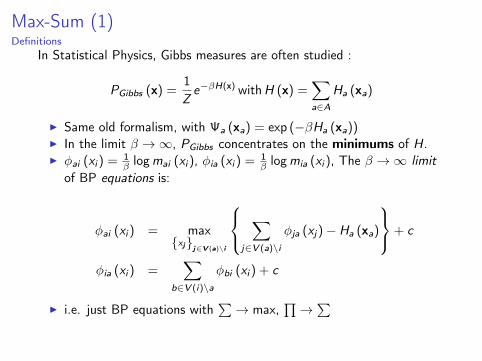
Max-Sum (1)Definitions

In Statistical Physics, Gibbs measures are often studied :

PGibbs (x) =1Ze−βH(x) withH (x) =

∑a∈A

Ha (xa)

I Same old formalism, with Ψa (xa) = exp (−βHa (xa))I In the limit β →∞, PGibbs concentrates on the minimums of H.I φai (xi ) = 1

β logmai (xi ), φia (xi ) = 1β logmia (xi ), The β →∞ limit

of BP equations is:

φai (xi ) = max{xj}j∈V (a)\i

∑j∈V (a)\i

φja (xj)− Ha (xa)

φia (xi ) =∑

b∈V (i)\a

φbi (xi ) + c

I i.e. just BP equations with∑→ max,

∏→∑

I Max Sum is exact on trees, if the solution is unique, argmaxφi (xi )for φi (xi ) =

∑b∈V (i) φbi (xi ) gives the optimum

∑a∈A

Ha (xa)

I Same old formalism, with Ψa (xa) = exp (−βHa (xa))

I In the limit β →∞, PGibbs concentrates on the minimums of H.I φai (xi ) = 1

of BP equations is:

∑j∈V (a)\i

φia (xi ) =∑

b∈V (i)\a

φbi (xi ) + c

∏→∑

∑a∈A

Ha (xa)

I Same old formalism, with Ψa (xa) = exp (−βHa (xa))I In the limit β →∞, PGibbs concentrates on the minimums of H.

I φai (xi ) = 1β logmai (xi ), φia (xi ) = 1

β logmia (xi ), The β →∞ limitof BP equations is:

∑j∈V (a)\i

φia (xi ) =∑

b∈V (i)\a

φbi (xi ) + c

∏→∑

∑a∈A

Ha (xa)

of BP equations is:

∑j∈V (a)\i

φia (xi ) =∑

b∈V (i)\a

φbi (xi ) + c

∏→∑

∑a∈A

Ha (xa)

of BP equations is:

∑j∈V (a)\i

φia (xi ) =∑

b∈V (i)\a

φbi (xi ) + c

∏→∑

∑a∈A

Ha (xa)

of BP equations is:

∑j∈V (a)\i

φia (xi ) =∑

b∈V (i)\a

φbi (xi ) + c

∏→∑

∑a∈A

Ha (xa)

of BP equations is:

∑j∈V (a)\i

φia (xi ) =∑

b∈V (i)\a

φbi (xi ) + c

∏→∑

Max Sum (2)MS for D-bounded Minimum Steiner Tree

I Input: Rooted graph G = (V ,E , r), edge costs{ce}e∈E , vertex prizes {bi}i∈V

I Problem: Find minT⊂G tree∑

e∈ETce −

∑i∈VT

Max Sum representation:

I Variables (di , pi ) associated to i ∈ V . 1 ≤ di ≤ Dand pi ∈ V (i) ∪ {∗} .

I Constraints on links: pi = j⇒ di = dj + 1 ∧ pj 6= ∗

I Cost: H (p,d) =∑

i∈V cipi where ci∗ = bi

1 2 3 4 5 6

7 8 9 10 11 12

e∈ETce −

∑i∈VT

1 2 3 4 5 6

7 8 9 10 11 12

e∈ETce −

∑i∈VT

1 2 3 4 5 6

7 8 9 10 11 12

e∈ETce −

∑i∈VT

1 2 3 4 5 6

7 8 9 10 11 12

e∈ETce −

∑i∈VT

1 2 3 4 5 6

7 8 9 10 11 12

e∈ETce −

∑i∈VT

1 2 3 4 5 6

7 8 9 10 11 12

Max-Sum (3)Optimality results

TheoremIf the min is unique, in a FP of Max Sum for the Minimum SpanningTree (i.e. D = N, T = V ) on arbitrary graphs,(p∗i , d

∗i ) = argmaxφi (pi , di ) define the optimum tree

Proof.(Sketch): Assume FP giving unoptimal solution on G , and consider thecomputation tree rooted at v ∈ V , Tk = (Vk ,Ek):

I Vk = {v = v1, . . . vl : l ≤ k, (vivi+1) ∈ E , vi+2 6= vi}I Ek = {(p1, p2) if p1 = p2v}I Tk is locally isomorphic to G , but Tk is a tree (covering)

I Vk = {v = v1, . . . vl : l ≤ k, (vivi+1) ∈ E , vi+2 6= vi}

I Ek = {(p1, p2) if p1 = p2v}I Tk is locally isomorphic to G , but Tk is a tree (covering)

I Vk = {v = v1, . . . vl : l ≤ k, (vivi+1) ∈ E , vi+2 6= vi}I Ek = {(p1, p2) if p1 = p2v}

I Tk is locally isomorphic to G , but Tk is a tree (covering)

Max-Sum (4)

General scheme:

1. FP of MS in G ↔ FP in Tk withappropriate leaf conditions

2. Tk is a tree =⇒ MS is exact on Tk

3. On Tk the [lifting of] {p∗i } defines a forestwith each connected component nottouching the leaves isomorphic to {p∗i } onG .

4. Take the optimal solution {qi} on G anduse it to improve the solution on Tk (byreplacing the pink CC) =⇒ contradiction

GTlift d i

lift d i

Max-Sum (4)

General scheme:

GTlift d i

lift d i

Max-Sum (4)

General scheme:

GTlift d i

lift d i

Max-Sum (4)

General scheme:

GTlift d i

lift d i

The End

Thanks, and happy holidays!

belief propagation for combinatorial...

Documents