BACHELORARBEIT

Titel der Bachelorarbeit

Bell's theorem and experimental tests

Verfasser

Cheng Xiaxi

Matrikelnummer: a0800812

Institut für Experimentalphysik der Universität Wien

angestrebter akademischer Grad

Bachelor of Science (B. Sc.)

Wien, im Juli 2011

Studienkennzahl lt. Studienblatt: 033676

Betreuer: Ao. Univ. -Prof. Dr. Reinhold A. Bertlmann

Contents

1 Introduction 3

2 Basic concepts of quantum mechanics 52.1 The density operator . . . . . . . . . . . . . . . . . . . . . . . 72.2 The entangled state . . . . . . . . . . . . . . . . . . . . . . . 8

3 Part I: Bell’s Theorem 93.1 Bell’s Theorem . . . . . . . . . . . . . . . . . . . . . . . . . . 93.2 The general argument (1964) . . . . . . . . . . . . . . . . . . 113.3 CHSH – The non-idealized case (1971) . . . . . . . . . . . . . 133.4 CH – more experiment related (1974) . . . . . . . . . . . . . 153.5 Wigner – a combinatorial analysis . . . . . . . . . . . . . . . 173.6 Relations between Bell’s inequality and entanglement witness 18

4 Part II: Experimental Tests 204.1 Requirement for general experimental tests . . . . . . . . . . 204.2 The “First” Generation . . . . . . . . . . . . . . . . . . . . . 224.3 The “Second” Generation . . . . . . . . . . . . . . . . . . . . 244.4 The “Third” Generation - G. Weihs, A. Zeilinger 1998 . . . . 274.5 Lab report . . . . . . . . . . . . . . . . . . . . . . . . . . . . . 29

4.5.1 Experimental requirements . . . . . . . . . . . . . . . 294.5.2 Setup and execution . . . . . . . . . . . . . . . . . . . 294.5.3 Results . . . . . . . . . . . . . . . . . . . . . . . . . . 334.5.4 Discussion . . . . . . . . . . . . . . . . . . . . . . . . . 36

5 Conclusion 37

6 Acknowledgement 38

2

Chapter 1

Introduction

We can say that one of the greatest philosophical and physical discussionswas caused by a single paper written by Einstein, Podolsky and Rosen[1](EPR) in 19351. In the paper, EPR assume reasonably the non-existence ofthe action-at-distance and define the criteria for a complete physical theory,which include the concepts of local causality and physical reality. By demon-strating mathematically their ideas within a though experiment, which wasmodified by Bohm[26] later on, they concluded that the description of quan-tum mechanics may be incomplete. This conclusion is formulated becausethis real, deterministic property isn’t contained in the formalism of quan-tum theory. And that is also the birth of the term of the “spooky action atthe distance[1].” The observation on one system immediately influences theobservation on the second one.Few months later, Bohr[2] replied to EPR and defended quantum mechanicswith his principle of complementarity. He denoted that the realistic view-point is inapplicable under the macroscopic level.In the following decades, in order to fulfill the desire of understanding na-ture, not only was the validation of contextuality in nature questioned, butalso the suggestions of extending quantum physics with a model of unknown“hidden” variable theory (HVT) for the completion were proposed. Manygreat physicists, e.g. Von Neumann, Gleason, Jauch and Piron, made someattempts to deny the theoretical extension. Apparently, all the proofs con-tain some leakages in their axioms or failed at the point of determinism andcongruence with quantum mechanics[3].Finally, both possible explanations were fully eliminated by the two follow-ing “no-go” theorems: the Kochen-Specker theorem and Bell’s theorem.The present work covers Bell’s theorem, published in 1964[4] by John Bell.He formulates a contradiction between the HVT and quantum mechanical

1Interestingly, the EPR paper became cited with a delay of 30 years, i.e., after Bellpublished his inequality and nowadays in the age of quantum information, there is anexponential increase of citations.

3

measurement. Besides the brief summaries of a few interesting proofs ofBell’s theorem, the most significant historical experimental tests of Bell’stheorem, during the last decades, are hereby also described and analysed.

4

Chapter 2

Basic concepts of quantummechanics

In this chapter, a short introduction into quantum mechanics will be ex-plained and all necessary mathematical notations for understanding thepresent work will also be mentioned.According to the fundamental law of quantum mechanics, a quantum stateφ of a given system is described by a complex function, called the wave func-tion, which contains the complete knowledge of the state and allows one todetermine the probabilities of obtaining certain measurement results madein the state. Suppose φ(~x, t) is a function of the space ~x and time t, thenthe probability of finding the system in the coordinate interval [~x, ~x+d~x] orshortly d3x at time t is given by

|φ(~x, t)|2d3x (2.1)

And due to the normalization condition, the total probability is:

||φ||2 =

∫|φ(~x, t)|2d3x = 1 = 〈φ|φ〉 (2.2)

where || · || =√〈 · | · 〉 and the right side of the equation is expressed by the

Dirac notation.To gain a deeper understanding of the quantum states, let us consider thespace underlying our physical objects, which is also called the Hilbert space.Definition: A Hilbert space H is a finite- or infinite-dimensional, linearvector space with the scalar product in C (Complex field). The inner productof the elements of the space, 〈φ|ψ〉 =

∫φ∗ψd3x, with φ, ψ ∈ H, satisfies the

following properties, where φ∗ is the complex conjugate of φ:

� 〈φ|ψ〉 is complexly conjugated:

〈φ|ψ〉 = 〈ψ|φ〉

where the term with overline denotes the complex conjugation.

5

� 〈φ|ψ〉 is linear in its second argument. For all complex number a andb:

〈φ|aψ1 + bψ2〉 = a〈φ|ψ1〉+ b〈φ|ψ2〉

� The inner product is positive definite:

〈φ|φ〉 ≥ 0

where the case of equality holds for φ = 0.

� The norm, a real-value function, is also defined by the inner product:

||φ|| =√〈φ|φ〉

Physical states expressed by wave functions obey the superposition princi-ples. If {|φi〉} are all possible states of H, then any linear combination |φ〉of them also belongs to H:

|φ〉 = c1|φ1〉+ c2|φ2〉+ ...+ cN |φN 〉 (2.3)

where {ci} are complex numbers and i = 1, 2, . . . N . |ci|2 gives the proba-bility of obtaining φi with

∑Ni=1 |ci|2 = 1:

|ci|2 = |〈φi|ψ〉|2 (2.4)

If {|φi〉} are orthonormal, they are called the orthonormal bases. Thereforea quantum state can be generally written as:

|φ〉 =

N∑i=1

ci|φi〉 (2.5)

The observables are operators which act on the wave function, if certainphysical quantities need to be measured. The measurement results are givenby the eigenstates of the corresponding observable with their eigenvalues.Imagine an operator A acting on any arbitrary eigenstate |φi〉, then:

A|φi〉 = λi|φi〉

where λi is the eigenvalue and denotes the measurement probability.The most important analysis of this work is based on the expectation valueof an observable. Since a statistical average value for the given observableacted on a large number of the identically prepared systems is required, thismean value is defined by the expectation value:

〈A〉φ =

∫φ∗Aφd3x = 〈φ|A|φ〉 =

N∑n,p=0

c†ncpAn,p (2.6)

where An,p = 〈φn|A|φp〉 is the matrix element of the observable A.

6

2.1 The density operator

Usually, we often deal with states of systems, which are not perfectly de-termined. In order to make the maximal use of this partial informationwe possess about the state of the system, the density matrix formalism isintroduced. The density operator ρ is therefore defined as:

ρ = |φ〉〈φ| (2.7)

Analogously, the expectation value is given by:

〈A〉φ = tr(ρ ·A) = tr(A · ρ) (2.8)

Andtr(ρ) = 1 (2.9)

For a given pure state |φ〉 whose information is perfectly known, the densityoperator has to fulfil the following properties:

ρ2 = ρ

ρ† = ρ

tr(ρ2) = 1

For the completeness, a mixed state is present when there is a statisticaldistribution of pure states. Since there is no interference effects betweenthe pure states, a mixed state can therefore only be given by the densityoperator:

ρ =∑i

pi|φi〉〈φi| =∑i

piρi (2.10)

where∑

i pi = 1 and {pi} are the probabilities of detecting {|φi〉〈φi|}. Thefollowing properties will be satisfied:

tr(ρ) =∑i

pitr(ρi)

tr(ρ) = 1

〈A〉φ = tr(ρ ·A)

ρ2 6= ρ

tr(ρ2) ≤ 1

Here the last inequality can be seen as a measure of the mixedness of a givenstate.

7

2.2 The entangled state

Before starting with Bell’s theorem, let us first take a brief look at theentangled state.We consider the following quantum state vector:

|Φ〉 = a · |x〉1 |y〉2 + b · e−iφ · |y〉1 |x〉2 (2.11)

which is a general form of an entangled state for two subsystems. Here, |a|2and |b|2 are the probabilities of the corresponding product states |x〉1⊗|y〉2 =|x〉1 |y〉2 and |y〉1⊗|x〉2 = |y〉1 |x〉2 with |a|2+ |b|2 = 1, the term e−iφ denotesa phase difference.The peculiar property of this kind of states is that they can’t be factorizedinto a product of two states of individual subsystems.In other words, a state vector |Ψ〉 in biparticle system describing, e.g., twosubsystems of photons can generally be written in the form:

|Ψ〉 =∑m,n

cm,n |m〉1 |n〉2 (2.12)

where cm,n = am · bn are the probability coefficients of |m〉1 |n〉2, am is them-th probability coefficient of the single photon state |Ψ1〉 =

∑mam |m〉, the

analogous notation bn for the other single photon.A state which can be written in Eq. (2.12) is called separable. Otherwise,the state is said to be entangled, which means:

cm,n 6= am · bn (2.13)

In conclusion, an entangled state can only be totally examined as a wholesystem. Therefore we define an entangled state as such a state with two ormore subsystems, separated by a certain distance, that the whole system,but not the individual subsystems, is well defined.The most remarkable entangled states are called Bell states, which havemaximal entanglement and are given for photons with horizontal and verticalpolarizations by: ∣∣Ψ+

⟩=

1√2

(|H〉1 |V 〉2 + |V 〉1 |H〉2) (2.14)

∣∣Ψ−⟩ =1√2

(|H〉1 |V 〉2 − |V 〉1 |H〉2) (2.15)

∣∣Φ+⟩

=1√2

(|H〉1 |H〉2 + |V 〉1 |V 〉2) (2.16)

∣∣Φ−⟩ =1√2

(|H〉1 |H〉2 − |V 〉1 |V 〉2) (2.17)

8

Chapter 3

Part I: Bell’s Theorem

3.1 Bell’s Theorem

Let us consider the following thought experiment made by Bohm[26] (EPRB).Suppose there is a source which is able to make pairs of particles with corre-lated property. Let’s say that the correlation is applied to their spins. Eachparticle has a spin of one half, but they do have a total spin of zero with anantisymmetric wave function, also called a singlet state, which is given bythe following Dirac notation:∣∣ψ−⟩ =

1√2

(|↑〉 |↓〉 − |↓〉 |↑〉) (3.1)

These particles are sent into reverse directions. When the particles areremote from one other, they will be detected by Stern-Gerlach appara-tuses, which simply deflect particles with a corresponding spin “up”-wardsor “down”-wards by the established inhomogeneous magnet field, whose ori-entations are freely adjustable, as shown in Fig. 3.1.The singlet state defined above simply describes that the possibility of mea-suring “up” in the detector system 1 and “down” in the system 2 is equalto the possibility of vice versa, if the magnet fields of both apparatuses arechosen to be parallel, e.g., to the z-axis.The perfect anti-correlation in this case leads us to suggest that the fun-damental laws of physics are deterministic. The “stochastic” measurementresults are the results of imperfect experimental setups. Therefore it wasvery reasonable to propose such a deterministic, unknown model to describethe quantum world, since this pre-determinism has not be considered in thequantum mechanical description. The only necessary property of these hid-den variable theories is the agreement between theoretical prediction andthe statistical reality. In the present chapter, we will discuss whether it ispossible to prove the existence of such theories with the latter requirement.First of all, let us analyze the correlation concerning the measurement of

9

EPRB experiment. Let us give the measurement results actual values of1 for photon deflected “up” and -1 for “down.” This correlation is indeednothing major in the case of parallel magnet field orientations. But whathappens when the fields are rotated by arbitrary angles α and β respectivelyfor systems 1 and 2? In other words, what is the correlation if the fields arerandomly orientated?If the measurement is repeated N times, from a classical point of view, we

Figure 3.1: EPRB thought experiment with Stern Gerlach apparatuses (Ref.[22])

will receive a correlation:

〈ab〉ψ− =∑j

ajbjN

(3.2)

where aj and bj are separately the measurement results in systems 1 and 2.A geometric illustration for this classic correlation is to image an unit vectorrepresenting the magnet field orientation in system 1, let us call it ~α, andthe analogous notation ~β for system 2. Suppose the planes, which ~α and ~βare separately perpendicular to, are disks, as shown in Fig. 3.2. From Eq.

Figure 3.2: The two disks divide the unit sphere into 4 parts, which rep-resent the correlation between the measurements. The shaded areas can beinterpreted as anti-correlation, while the rest as correlation. (Ref. [9])

10

(3.2) we obtain the classical correlation:

〈ab〉ψ− =θ − (π − θ)

π= −1 +

2θ

π(3.3)

Let us now return to the statistical prediction of quantum mechanics. Themeasurements of each particle are done by the observables ~α~σ1 and ~β~σ2,respectively. Hence, the correlation is given by:

〈ab〉ψ− =⟨~α~σ1 ⊗ ~β~σ2

⟩ψ−

= −~α~β = −cosθ (3.4)

where θ is the angle difference between the ~α and ~β and the σ are the Paulimatrices.We see Eq. (3.3) only partially reproduces quantum mechanical results ofEq. (3.4) at θ = 0; π/2 and π.This is one of the very first peculiar examples concerning the differencebetween local, deterministic theories and statistical prediction of quantummechanical theories.

3.2 The general argument (1964)

Actually, from Eq. (3.4) we are able to calculate the quantum mechanicalprediction for the expectation value of the observable ~α~σ1 ⊗ ~β~σ2:

[E(~α, ~β)]ψ− =⟨~α~σ1 ⊗ ~β~σ2

⟩ψ−

= −~α~β (3.5)

One critical assumption, which Bell’s derivation relies on, is the special caseof Eq. (3.5):

[E(~α, ~α)]ψ− = −1 (3.6)

which contains the deterministic property of this idealized system that thedetected samples have to be perfectly correlated.Since a local, realistic interpretation of quantum mechanics is requested, buta quantum state can’t be determined for an individual measurement, onehas to assume a more advanced specification, in which the determinism isbuilt.In this case, Bell introduced a “hidden” variable λ, which he hasn’t madeany restriction for, either in its dimension or in its construction. Propertiesof this will be demonstrated below:If we repeat the spin measuring in the given thought experiment, we will seethe unsurprisingly correlated results. The possibility P (A,B|~α, ~β) that A asmeasured result in system 1 with field orientation ~α and B in system 2 with~β, can’t be factorized into P1(A, ~α) ·P2(B, ~β). That means that a certaincorrelation can’t be locally explained without “action-at-a-distance”.By applying λ, we claim the following:

P (A,B|~α, ~β, λ) = P1(A, ~α, λ) ·P2(B, ~β, λ) (3.7)

11

This is a hypothesis of local causality or “no-action-at-distance”. In orderto make this local theory congruent with quantum mechanical results, λ isintroduced. Therefore this variable, which we don’t know, can be seen asa supplement for quantum mechanics. In order to define the probabilityof measurements for an ensemble, Bell defined intuitively the distributionfunction for λ: ∫

dλρ(λ) = 1 (3.8)

If ρ(λ) is a normalized probability distribution, the expectation value of ajoint spin measurement at ~α and ~β can be written as:

E(~α, ~β) =

∫ρ(λ)A(~α, λ)B(~β, λ)dλ (3.9)

where A(~α, λ) = ±1 and B(~β, λ) = ±1.According to the conditions of the hidden-variable theory, the above equa-tion has to be equal to Eq. (3.5). From Eq. (3.6),

A(~α, λ) = −B(~α, λ) (3.10)

has to hold. Assuming the correctness of Eq. (3.9), we obtain Eq. (3.11) bysubstituting Eq. (3.10) into Eq. (3.9):

E(~α, ~β) = −∫ρ(λ)A(~α, λ)A(~β, λ)dλ (3.11)

By introducing a third field orientation ~γ, we have

E(~α, ~β)− E(~α,~γ)

= −∫ρ(λ)[A(~α, λ)A(~β, λ)−A(~α, λ)A(~γ, λ)]dλ

= −∫ρ(λ)A(~α, λ)A(~β, λ)[1−A(~β, λ)A(~γ, λ)]dλ

(3.12)

Since A,B = ±1, the equation above turns to the following inequality:

|E(~α, ~β)− E(~α,~γ)| ≤∫ρ(λ)[1−A(~β, λ)A(~γ, λ)]dλ (3.13)

And finally,|E(~α, ~β)− E(~α,~γ)| ≤ 1 + E(~β,~γ) (3.14)

This is the original form of Bell’s inequality.If a theory described by a local, deterministic hidden variable is true, theinequality above will hold. But a simple test by using Eq. (3.5) and tak-ing ~α, ~β and ~γ to be coplanar as well as taking account of the followingconditions:

~α · ~β = ~β ·~γ =1

2

~α~γ = −1

2

(3.15)

12

leads to a mathematical contradiction:

|E(~α, ~β)− E(~α,~γ)| = 1 ≤ 1

2= 1 + E(~β,~γ) (3.16)

This version of Bell’s theorem, as just proved, can be summarized as follows:No deterministic hidden-variable theory satisfying Eq. (3.6) andthe locality condition Eq. (3.9), can agree with all of the predic-tions by quantum mechanics concerning the spin of a pair spin-12particles in the singlet state.1

3.3 CHSH – The non-idealized case (1971)

A physical theory can’t be considered valid as long as it is not proven exper-imentally. The very first Bell’s inequality Eq. (3.14) describes the idealizedcase, which strongly depends on Eq. (3.6). In fact, this condition can’t holdfor actual experiments because any state analyzer will always have someleakages for some reason. Therefore it is outrageously difficult to be real-ized in the lab. Exactly these problems are approached by Clauser, Horne,Shimony and Holt[5] (CHSH), who extended the Bell’s inequality for thenon-deterministic case, which doesn’t depend on the mentioned critical con-dition Eq. (3.6).Here the measurement results A(~α, λ) and B(~β, λ) in systems 1 and 2 wererespectively assigned as the following:

|A(~α, λ)| ≤ 1 (3.17)

|B(~β, λ)| ≤ 1

≤ 1 also includes the non-idealized case, when +1 for detecting “up”, -1 for“down” and 0 for blank.The locality condition is still included in the expectation values given in Eq.(3.9). Now consider the following expression:

E(~α, ~β)− E(~α, ~β′) =∫ρ(λ)[A(~α, λ)B(~β, λ)−A(~α, λ)B(~β′, λ)]dλ

This can be written as:

E(~α, ~β)− E(~α, ~β′) =

∫ρ(λ)A(~α, λ)B(~β, λ)[1±A(~α′, λ)B(~β′, λ)]dλ

−∫ρ(λ)A(~α, λ)B(~β′, λ)[1±A(~α′, λ)B(~β, λ)]dλ

1J. F. Clauser, A. Shimony, Rep.Prog.Phys. 41 1881 (1978)

13

where ~α, ~α′, ~β and ~β′ are all different field orientations.By applying Eq. (3.17) and the triangle inequality, we have:

|E(~α, ~β)− E(~α, ~β′)| ≤∫ρ(λ)[1±A(~α′, λ)B(~β′, λ)]dλ+

∫ρ(λ)[1±A(~α′, λ)B(~β, λ)]dλ

or|E(~α, ~β)− E(~α, ~β′)| ≤ ±|E(~α′, ~β′) + E(~α′, ~β)|+ 2

Therefore the CHSH inequality is:

|E(~α, ~β)− E(~α, ~β′)|+ |E(~α′, ~β) + E(~α′, ~β′)| ≤ 2 (3.18)

Mathematically, this inequality can be easily violated if we take the fourvectors above to be coplanar with an included angle of π/4. Hence, thequantum mechanical limit of violation of Bell’s inequality is given by:

|E(~α, ~β)− E(~α, ~β′)|+ |E(~α′, ~β) + E(~α′, ~β′)| = 2√

2 (3.19)

2√

2 > 2

On the other hand, if the condition of perfect correlation Eq. (3.6) holds,CHSH Eq. (3.19) implies the original Bell’s inequality Eq. (3.14) as a spe-cial case.Surely, CHSH inequality isn’t the universal solution of all problems. Gener-ally, the following four different cases of the observation are possible whendetecting particles passing through some analyzer: a) both particles are ob-served, b) only particle one is observed, c) only particle two is observed, d)none of them are observed. Clearly, the probability density distribution ρ ofthe union of these four sub-ensembles is independent of setting angles ~α and~β of the analyzers, but on the collimator and source geometry. However,the mode of partitioning of the measurement results may well depend onthe angle. Therefore there is no reason to assume that the composition anddistribution of each sub-ensemble has no angle dependence.Since the normalization of ρ, see Eq. (3.8) is used in the derivation, theexpectation of the independence of ~α and ~β of ρ has to be made. Thereforethe ensemble for which ρ is defined must also include unobserved particles.Because the number of unobserved particles is unknown, a comparison ofCHSH with experimental evidence would be inadequate. Exactly, this factis considered by Clauser and Horne[6], which will be discussed in the nextchapter. They derived an inequality from the hypothesis of locality anddeterminism or realism, in which only the ratios of the detection propertiesare used and the crucial condition of Eq. (3.8) is not required.

14

3.4 CH – more experiment related (1974)

Clauser and Horne[6] (CH) found another inequality, which has a weakerassumption than CHSH. Therefore it is performable in an actual experi-ment. First of all, consider the apparatus configuration given in Fig. 3.3Suppose the adjustable values for the orientations of apparatuses 1 and 2

Figure 3.3: The basic idea of an experiment on Bell’s theorem: The sourceemits a pair of correlated particles, which are analyzed by two apparatuses.Each apparatus consists of an analyzer, whose orientation is adjustable, anda detector, which is able to measure the rate of the counts. Comparing bothmeasurement results yields the number of coincidence. (Ref. [10])

are described by α and β respectively. Suppose N is the total number ofpaired correlated particles emitted by the source, during a given integrationtime. N1(α) and N2(β) describe separately the number of counts in system1 with α and system 2 with β. N12(α, β) is the number of simultaneousdetection(coincidence) in system 1 and 2. Further more, the possibilities forthese results are given by:

p1(α) = N1(α)/N

p2(β) = N2(β)/N

p12(α, β) = N12(α, β)/N

(3.20)

if N is sufficiently large.By applying the hidden variable λ, we assume that α, β, λ, p1 and p2 areindependent and we also demand the following relation:

p12(α, β, λ) = p1(α, λ) · p2(β, λ) (3.21)

15

The averaged probabilities above are then intuitively given by:

p1(α) =

∫ρ(λ)p1(α, λ)dλ

p2(β) =

∫ρ(λ)p2(β, λ)dλ

p12(α, β) =

∫ρ(λ)p1(α, λ)p2(β, λ)dλ

(3.22)

which are then not depended on the unknown variable.After using the lemma 2 proved by Clauser and Horne[6] and the assumption:

0 ≤ pi(λ, α) ≤ pi(λ,∞) ≤ 1 (3.24)

which denotes that the probability of detecting a photon after a polarizer isalways less or equal to the case with the removed analyzer, the inequalitycan be written in the following:

−p12(∞,∞) ≤p12(λ, α, β)− p12(λ, α, β′)+p12(λ, α

′, β) + p12(λ, α′, β′)

−p12(λ, α′,∞)− p12(λ,∞, β) ≤ 0

(3.25)

After averaging and building the ratio of probabilities, we receive the CH-inequality:

p12(α, β)− p12(α, β′) + p12(α′, β) + p12(α

′, β′)

p12(α′,∞) + p12(∞, β)

=R(α, β)−R(α, β′) +R(α′, β) +R(α′, β′)

R12(α′,∞) +R12(∞, β)≤ 1

(3.26)

where R denotes the rate of counts of coincidence, which is proportionalto the number of detected particles, and terms including ∞ stand for thecoincidence rate of detection when the corresponding analyzer is removed.As we see, the assumption that the total number N of emitted particles is inthis case irrelevant, rules out one of the practical impossibilities of detection.In order to complete the proof of the theorem, let us consider, e.g., the de-tection of spin-correlated photons given in Eq. (2.16) with linear polarizers.By introducing the quantum mechanical probability into the CH-inequality,

pqm12 (α, β) =|[(1〈H|cosα+1 〈V |sinα)⊗ (2〈H|cosβ +2 〈V |sinβ)] ·

1√2

[|H〉1|H〉2 + |V 〉1|V 〉2]|2

=1

4(1 + cos2(β − α))

(3.27)

2if x, x′, y, y′, X, Y are real numbers such that 0 ≤ x,x′ ≤ X and 0 ≤ y, y′ ≤ Y , thenthe inequality:

−XY ≤ xy − xy′ + x′y + x′y′ − Y x′ −Xy ≤ 0 (3.23)

holds.

16

where α and β are the angles of the polarizers. The probability of detectingone photon is simply 1

2 . By choosing α = 0◦, β = 22.5◦, α′ = 45◦ andβ′ = 65.5◦, the violation yields out:

pqm12 (α, β)− pqm12 (α, β′) + pqm12 (α′,β) + pqm12 (α′, β′)− pqm1 (α′)− pqm2 (β) =√

2− 1

2≤ 0

(3.28)

which is clearly a contradiction.By adding symmetry consideration from quantum mechanical predictionsthe CH-inequality can be specified for the following conditions:

p1(α) = const.

p2(β) = const.

p12 = f(|β − α|)

and after choosing:

|α− β| = |α′ − β′| = |α′ − β| = 1

3|α− β′| = φ

we receive the following inequality given by S(φ):

S(φ) ≡ 3p12(φ)− p12(3φ)

p1 + p2≤ 1 (3.29)

At first sight, the inequality above seems to be elegant because of the smallnumber of measurements. But the truth is that fulfilling the necessarycondition requires many more measurement procedures.

3.5 Wigner – a combinatorial analysis

This version of Wigner’s inequality is derived by pure combinatorial analysis[7],where perfect anti-correlation and perfect detection efficiency are assumed.Let us first consider the familiar EPR experiment and suppose there arethree possible detection parameters such as A, B and C with the possiblemeasurement result of + or −. By assuming the locality condition, we canconstruct the following combinations of measurement results in Table 3.1.Since the numbers of counts are positive, the following inequality must hold:

N3 +N4 ≤ (N2 +N4) + (N3 +N7) (3.30)

Further, the probability of measuring + in one detector with the setting Aand + in the other detector with the setting B is given by:

p(A+, B+) =N3 +N4

N(3.31)

17

The number of counts Particle 1 Particle 2

N1 (A+, B+, C+) (A−, B−, C−)

N2 (A+, B+, C−) (A−, B−, C+)

N3 (A+, B−, C+) (A−, B+, C−)

N4 (A+, B−, C−) (A−, B+, C+)

N5 (A−, B+, C+) (A+, B−, C−)

N6 (A−, B+, C−) (A+, B−, C+)

N7 (A−, B−, C+) (A+, B+, C−)

N8 (A−, B−, C−) (A+, B+, C+)

Table 3.1: Possible combinations of measurement results

where N =∑8

i Ni is the total number of counts. Analogously, we have:

p(A+, C+) =N2 +N4

N

p(C+, B+) =N3 +N7

N

By applying the relations above into Ineq. (3.30), we obtain the Wigner’sinequality:

p(A,B) ≤ p(A,C) + p(C,B) (3.32)

Another path of derivation of Wigner’s inequality is to make use of thediscrete expectation value of correlation, such as:

E(A,B) = p(A+, B+) + p(A−, B−)− p(A+, B−)− p(A−, B+) (3.33)

where∑

i pi = 1.A contradiction results, when the probability for correlation is, e.g., givenby:

p(A,B) = |(〈A+ | ⊗ 〈B + |)|ψ−〉|2 =sin2(

6 (A,B)2 )

2(3.34)

and if we chose the following angles: 6 (A,B) = 60◦, 6 (B,C) = 60◦ and6 (A,C) = 120◦.

3.6 Relations between Bell’s inequality and entan-glement witness

In this last section of the part I, an extended feature of Bell’s inequalitywill be briefly sketched. Let us recall the definition of entangled states. Ingeneral, a state in bi-particle system is said to be separable if and only if itcan be written as:

ρ =∑i

pi|φi〉A〈φi| ⊗ |φi〉B〈φi| (3.35)

18

where∑

i pi = 1 and 0 ≤ pi ≤ 1. Otherwise the state is entangled. Sincethis criterion is often very complicated to be tested, many methods areconstructed to distinguish between separable and entangled states.One foundational method of quantum entanglement theory is the so-calledentanglement witness. It is a Hermitian operator W , which is defined forseparable states ρsepA,B by:

tr(ρsepA,B ·W ) ≥ 0 (3.36)

and for entangled states ρentA,B by:

tr(ρentA,B ·W ) < 0 (3.37)

According to the fact that separable states do not violate Bell’s inequality,one is able to construct an entanglement witness upon the CHSH inequality.Let us first of all represent Eq. (3.19) by

tr(BCHSHρ) ≤ 2 (3.38)

where BCHSH is the CHSH operator defined by

BCHSH = ~α ·~σ ⊗ (~β + ~β′) ·~σ + ~α′ ·~σ ⊗ (~β − ~β′) ·~σ (3.39)

with ~σ = (σx, σy, σz)T . Therefore an entanglement witness WCHSH basing

on the CHSH inequality is given by:

WCHSH = 2 · I +BCHSH (3.40)

WCHSH does not only determine whether a state is entangled or separablebut also tests the local realism. By applying the Bell states(Eq. (2.14) -(2.17)), tr(WCHSH · ρ) fulfils the condition, Eq. (3.37), and violates Eq.(3.38). However, the entanglement witness based on Eq. (3.40) is not opti-mal, see Ref. [11].

19

Chapter 4

Part II: Experimental Tests

Since the correctness of quantum mechanics has been confirmed in a varietyof experimental situations in, e.g., nuclear and atomic physics, the ratherrare disagreement found by Bell seems to be a duty for many physiciststo experimentally test because the spatially separate systems may be thegreatest vulnerability of quantum physics.In the past thirty years, a great number of Bell test experiments has beenperformed. In order to rule out the local, realistic hidden-variable theory,ideas were created to raise the equipment efficiencies with improving tech-nology and to close the existing “loopholes.”

4.1 Requirement for general experimental tests

Until now, experimental results without any auxiliary assumptions don’texist. In the real-life experiments, the efficiency of the apparatus has to beconsidered, therefore a reasonable extension of the inequality is to implicatethe apparatus efficiencies.But generally, for a direct experimental violation, we experimentally requireat least:

� A source of a discrete state system which can be detected with highefficiency.

� High purity of the state. From the viewpoint of quantum mechanics,at least a strong correlation of each pair has to be achieved.

� High analyzer efficiency of transmission to allow states and reject allnearby unwanted states.

� Very high efficiency of transmission/absorption of the spectrum filter.

� Locality: the adjustable values of the apparatuses have to be quicklychanged, so that any kind of information transfer isn’t possible. Inother words, the space-like separation needs to be created.

20

Any absence of mentioned specifications will prevent the violation of Bell’stheorem. The dependence of the experiment on these specifications is demon-strated by the following three cases:

� Case I: nearly ideal, the efficiencies of the apparatuses are near 1. Inthis case, a wide range violation can be found.

� Case II: entirely poor apparatus efficiency, which leads to flattenedcurve around 0. This is especially the case in low energy cascadephoton experiments.

� Case III: weak correlation, impure states with depolarization or par-tially low efficiency of the apparatuses.

These cases are schematized in the following Fig. 4.1:

Figure 4.1: The curves are collected by violating the CH inequality withsymmetry consideration S(φ) ≤ 1. (Ref. [10])

Indeed, as we see, an experimental violation of Bell’s inequality has to beprepared carefully since the contrast of the curve observed in Fig. 4.1 dropsdown drastically at low efficiencies for partial experimental equipment.By introducing an auxiliary assumption for rescaling the curve, the violationcan be reached. Therefore measuring the efficiency coefficients of the experi-ment apparatuses becomes one of the most crucial points of all experiments.Besides improving technology, some of the experimental requirements canbe fulfilled and some are still open. Since the experimental goal is to elimi-nate the possibility of an interpretation of the “hidden” variable theory byviolating Bell’s inequality, one has to consider additional conditions for theexperiment, also called “loopholes.” In other words, loopholes exist when weare not able to eliminate the theory of the “hidden” variable.

21

Let us in the following summarize the most critical additional assumptions(loopholes), which scientists have ever tried to eliminate:

� Einstein - locality: The distance between the two detectors should belarge enough, so that any kind of exchange of information between themeasuring systems below or equal to the speed of light isn’t possible.

� Free choice: suppose a periodical procedure would reveal the infor-mation of the particles, we need a random choice machine to selectthe basis of measurement. Otherwise the information can be releasedbefore the measurement is executed.

� Fair sample: the detected samples represent the total ensemble of theparticles emitted by the source. (The detection efficiency is alwayslower than 100% in an optical experiment. Calculation[8] shows thatthe violation doesn’t hold for a detection efficiency below 82%.)

In the chapters below, I only restrict the content to optical experimentsbecause of the remarkableness. Hence, a clear evolution of experimentalverification is introduced. In the so called “three generations” of Bell ex-periments, the unexplored loopholes were step by step closed with modernmethods.

4.2 The “First” Generation

The very first published Bell test experiment with entangled photons isperformed by Stuart J. Freedman and John F. Clauser[14] in 1972. In theirexperiment, they measured the two photons emitted by the exited Calciumatoms at a cascade decay. By making the following assumptions:

� The two photons propagate as separated localized particles,

� A binary selection (transmission or no-transmission) measurement foreach photon,

� The probability of detecting a photon is independent of transmissionof the polarizers,

they were able to show a clear violation of Bell’s inequality. The experimen-tal setup is sketched in the Fig. 4.2. A calcium atom beam effused from atantalum oven. The output of 227 nm wavelength of a deuterium arc lampis focused on the Ca beam. After the resonance absorption, the Ca atomsare excited to the 3d4p1P1. Only 7 % of the atoms, which do not decaydirectly back to the ground state, decay first of all to the 4p2 1S0. Beforethey reach the ground state, there exists an intermediate state 4p4s1P1, seeFig. 4.3. Two photons of 551 nm and 422 nm were emitted during this

22

Figure 4.2: Schematic setup of Freedman and Clauser (Ref. [14])

Figure 4.3: Calcium energy levels (Ref. [14])

23

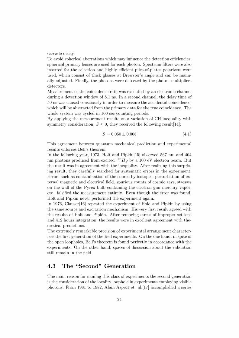
cascade decay.To avoid spherical aberrations which may influence the detection efficiencies,spherical primary lenses are used for each photon. Spectrum filters were alsoinserted for the selection and highly efficient piles-of-plates polarizers wereused, which consist of thick glasses at Brewster’s angle and can be manu-ally adjusted. Finally, the photons were detected by the photon-multipliersdetectors.Measurement of the coincidence rate was executed by an electronic channelduring a detection window of 8.1 ns. In a second channel, the delay time of50 ns was caused consciously in order to measure the accidental coincidence,which will be abstracted from the primary data for the true coincidence. Thewhole system was cycled in 100 sec counting periods.By applying the measurement results on a variation of CH-inequality withsymmetry consideration, S ≤ 0, they received the following result[14]:

S = 0.050± 0.008 (4.1)

This agreement between quantum mechanical prediction and experimentalresults enforces Bell’s theorem.In the following year, 1973, Holt and Pipkin[15] observed 567 nm and 404nm photons produced from excited 198Hg by a 100 eV electron beam. Butthe result was in agreement with the inequality. After realizing this surpris-ing result, they carefully searched for systematic errors in the experiment.Errors such as contamination of the source by isotopes, perturbation of ex-ternal magnetic and electrical field, spurious counts of cosmic rays, stresseson the wall of the Pyrex bulb containing the electron gun mercury vapor,etc. falsified the measurement entirely. Even though the error was found,Holt and Pipkin never performed the experiment again.In 1976, Clauser[16] repeated the experiment of Hold and Pipkin by usingthe same source and excitation mechanism. His very first result agreed withthe results of Holt and Pipkin. After removing stress of improper set lensand 412 hours integration, the results were in excellent agreement with the-oretical predictions.The extremely remarkable precision of experimental arrangement character-izes the first generation of the Bell experiments. On the one hand, in spite ofthe open loopholes, Bell’s theorem is found perfectly in accordance with theexperiments. On the other hand, spaces of discussion about the validationstill remain in the field.

4.3 The “Second” Generation

The main reason for naming this class of experiments the second generationis the consideration of the locality loophole in experiments employing visiblephotons. From 1981 to 1982, Alain Aspect et. al.[17] accomplished a series

24

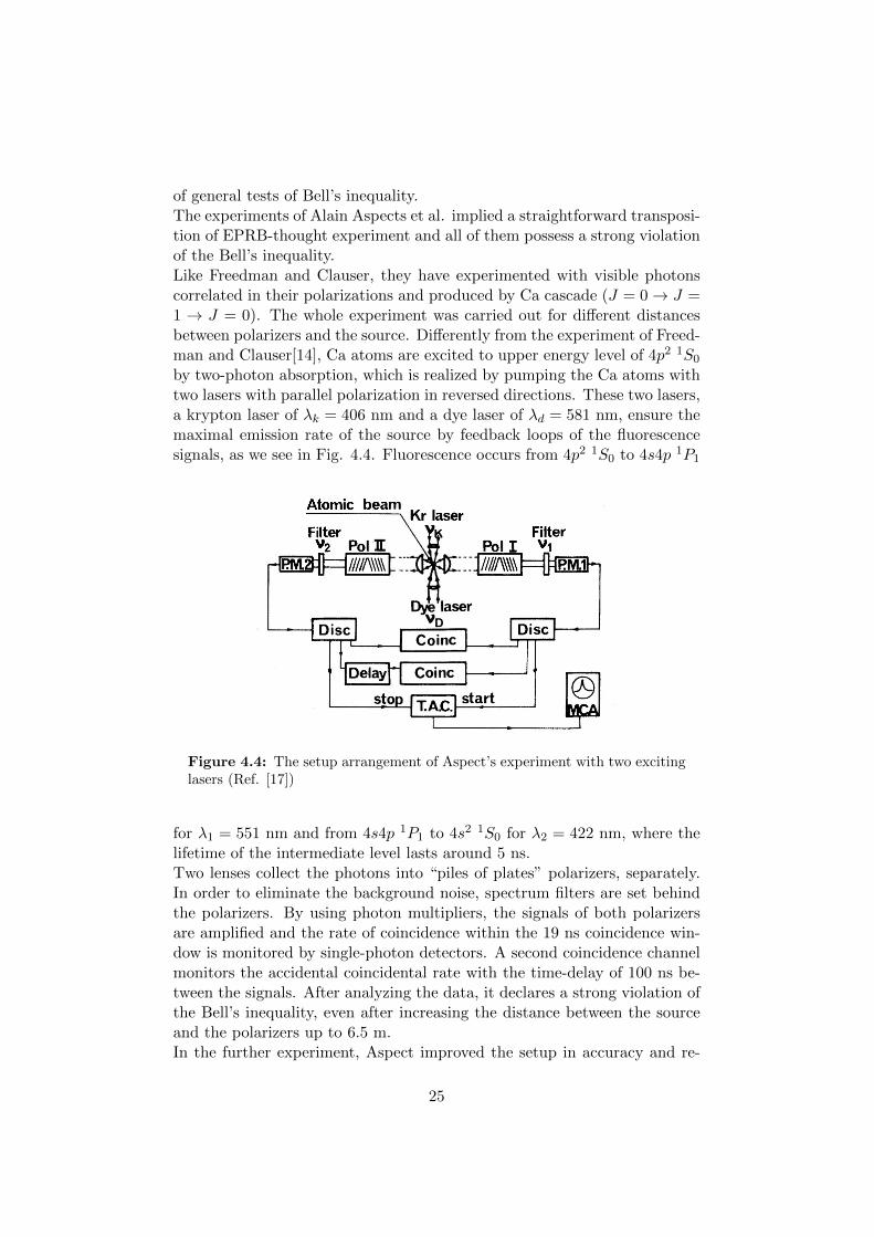
of general tests of Bell’s inequality.The experiments of Alain Aspects et al. implied a straightforward transposi-tion of EPRB-thought experiment and all of them possess a strong violationof the Bell’s inequality.Like Freedman and Clauser, they have experimented with visible photonscorrelated in their polarizations and produced by Ca cascade (J = 0→ J =1 → J = 0). The whole experiment was carried out for different distancesbetween polarizers and the source. Differently from the experiment of Freed-man and Clauser[14], Ca atoms are excited to upper energy level of 4p2 1S0by two-photon absorption, which is realized by pumping the Ca atoms withtwo lasers with parallel polarization in reversed directions. These two lasers,a krypton laser of λk = 406 nm and a dye laser of λd = 581 nm, ensure themaximal emission rate of the source by feedback loops of the fluorescencesignals, as we see in Fig. 4.4. Fluorescence occurs from 4p2 1S0 to 4s4p 1P1

Figure 4.4: The setup arrangement of Aspect’s experiment with two excitinglasers (Ref. [17])

for λ1 = 551 nm and from 4s4p 1P1 to 4s2 1S0 for λ2 = 422 nm, where thelifetime of the intermediate level lasts around 5 ns.Two lenses collect the photons into “piles of plates” polarizers, separately.In order to eliminate the background noise, spectrum filters are set behindthe polarizers. By using photon multipliers, the signals of both polarizersare amplified and the rate of coincidence within the 19 ns coincidence win-dow is monitored by single-photon detectors. A second coincidence channelmonitors the accidental coincidental rate with the time-delay of 100 ns be-tween the signals. After analyzing the data, it declares a strong violation ofthe Bell’s inequality, even after increasing the distance between the sourceand the polarizers up to 6.5 m.In the further experiment, Aspect improved the setup in accuracy and re-

25

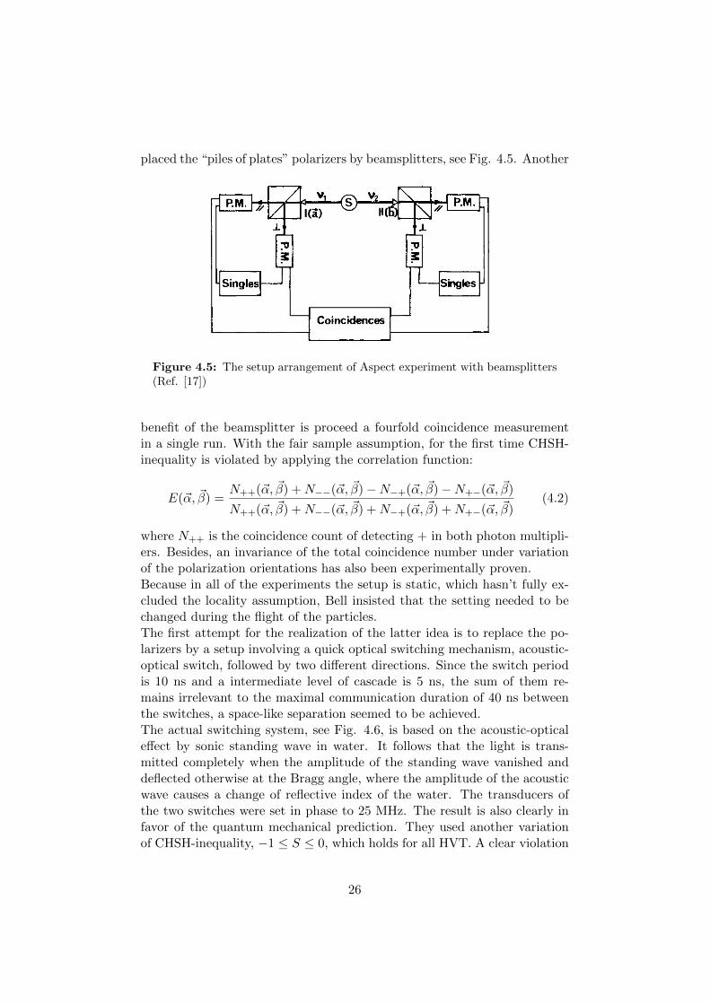
placed the “piles of plates” polarizers by beamsplitters, see Fig. 4.5. Another

Figure 4.5: The setup arrangement of Aspect experiment with beamsplitters(Ref. [17])

benefit of the beamsplitter is proceed a fourfold coincidence measurementin a single run. With the fair sample assumption, for the first time CHSH-inequality is violated by applying the correlation function:

E(~α, ~β) =N++(~α, ~β) +N−−(~α, ~β)−N−+(~α, ~β)−N+−(~α, ~β)

N++(~α, ~β) +N−−(~α, ~β) +N−+(~α, ~β) +N+−(~α, ~β)(4.2)

where N++ is the coincidence count of detecting + in both photon multipli-ers. Besides, an invariance of the total coincidence number under variationof the polarization orientations has also been experimentally proven.Because in all of the experiments the setup is static, which hasn’t fully ex-cluded the locality assumption, Bell insisted that the setting needed to bechanged during the flight of the particles.The first attempt for the realization of the latter idea is to replace the po-larizers by a setup involving a quick optical switching mechanism, acoustic-optical switch, followed by two different directions. Since the switch periodis 10 ns and a intermediate level of cascade is 5 ns, the sum of them re-mains irrelevant to the maximal communication duration of 40 ns betweenthe switches, a space-like separation seemed to be achieved.The actual switching system, see Fig. 4.6, is based on the acoustic-opticaleffect by sonic standing wave in water. It follows that the light is trans-mitted completely when the amplitude of the standing wave vanished anddeflected otherwise at the Bragg angle, where the amplitude of the acousticwave causes a change of reflective index of the water. The transducers ofthe two switches were set in phase to 25 MHz. The result is also clearly infavor of the quantum mechanical prediction. They used another variationof CHSH-inequality, −1 ≤ S ≤ 0, which holds for all HVT. A clear violation

26

Figure 4.6: Acoustic-optical switches (Ref. [17])

yielded out[17]:S = 0.101± 0.020 (4.3)

with a theoretical prediction of SQM = 0.112. The additional assumptionswhich have to be made are sufficiently high detector efficiency and fair de-tected samples of all emitted pairs. Until this point, it seemed the localityloophole is eliminated at first.

4.4 The “Third” Generation - G. Weihs, A. Zeilinger1998

This experiment definitely implements the ideas behind the experiments ofAlain Aspect et al.. In the experimenter’s view, the usage of the acoustic-optical switches, which is applied by a sinusoidal voltage, hadn’t successfullyruled out the locality assumption. The periodical change of the applied volt-age could somehow be predicted after all. Furthermore, distances and switchfrequency have been chosen unfortunately1, see Ref. [12, 13]. Thus commu-nication at the speed of light or even slower than the speed of light couldtheoretically explain the obtained results.For the first time, the experiment of G. Weihs[18] fully eliminated the lo-cality assumption with entangled photons in their polarizations. In theirexperiment, the two detectors, so called “Alice” and “Bob,” were separatedby a distance of 400 meters for the space-like separation. To prevent anycommunication obeying Einstein’s locality, the measurement duration waskept at 100 ns, which is clearly shorter than 1.3 µs, the duration of the

1A. Zeilinger, Phys. Lett. lISA, 1 (1986)

27

communication between the detectors.The entangled photons are produced by a BBO(β-BaB2O4) negative uni-axial birefringent crystal (ne < no) with the type II spontaneous parametricdown-conversion (SPDC - type II) pumped by a laser. SPDC - type II isa reverse process of the second harmonic generation (SHG), which is ableto downconvert one pump photon (E = 2hω0) in ex-ordinary polarizationinto two identical photons (E = hω0), one in ordinary and the other inex-ordinary polarization under the laws of conservation of energy and mo-mentum.However, the BBO crystal has a disadvantage. Due to birefringence of thecrystal, a route difference exists for ordinary and ex-ordinary wave in theBBO (ne < no), called the “walk-off” effect. Because this effect can de-stroy the condition for the entanglement, compensating systems includingthe same cutting but thinner BBO are introduced to cancel the difference.One of the key elements of this experiment is the selection of an analyzerdirection which completely processes unpredictably by a random numbergenerator. The actual selection is caused by an electric-optical modulator,which changes the polarization of the light by applied voltage. In this ex-periment, a random number generator is responsible for the random changein voltage. In general, such a machine can be seen as a background noisegenerator. In this case, the basic idea is to send single photons of a weaklight-emitting diode into a beamsplitter. Signals will be received either inone or in the other detector. Two photo-multipliers convert the weak sig-nal into digital “0” or “1.” And finally, these signals are connected with aflipflop, as shown in Fig. 4.7. The output of the random number generator

Figure 4.7: The basic idea of the quantum random number generator (Ref.[22])

controls the applied voltage of the electric-optical modulator, which is ableto change the photon polarization within a defined range.After measurement and calculation of the expectation values from coinci-

28

dence for the CHSH-inequality, a strong violation[18] of

S = 2.73± 0.02 (4.4)

agrees very well with quantum mechanical predictions.It still seems unlikely, that the local, realistic theory can be completely aban-doned because of other existing loopholes. In 2008, Salart et al.[23] enforcedagain the non-local argument with a separation of 18 km between the de-tectors in the Bell test experiment. In 2009, Ansmann et al.[24] seemed toovercome the greatest loophole, the detection loophole, with superconduct-ing qubits, but the separation condition wasn’t fulfilled.

4.5 Lab report

The present chapter contains a lab report of a self-made Bell test experi-ment in the framework of “Praktikum III: Quantenoptik” of the universityof Vienna. It describes the basic experimental technique in alignment ofoptical elements. By assuming the locality and detection efficiency, we alsosuccessfully violate the CHSH-inequality. In conclusion, this experiment canonly be considered as an introduction to quantum information experiments.But it surely awakes our interests in this field.

4.5.1 Experimental requirements

� BBO-crystal (Type II)

� 2 compensating BBOs (Type II)

� A Half-wave-plate

� A Pump laser (404 nm, max. 50 mW)

� 2 Polarizers

� 2 Detectors with single mode fiber coupling

� 2 Laserdiods (630 - 680 nm, max 5 mW)

� Diverse optical components

4.5.2 Setup and execution

The key to every highly sensitive measurement is the setting. If the setuphas been done carefully, the result will also be more acceptable. First of all,we have to keep one thing in mind, which is to take as much time as possibleto do the setup. The construction of our experiment isn’t very complicated,as shown in Fig. 4.8. The very first step is to set up the pump beam. To

29

Figure 4.8: The setup: After two steering mirrors (M1,M2), the pump beam(404 nm, V-polarized) is focused into the BBO crystal (optical axis is in thevertical plane) by a lens of 6 cm focal length to create a pair of entangledphotons (808 nm). The two 808 nm beams, which propagate along the lineswhich are 3◦ from the pump line horizontally, are deflected to left and rightby two prism mirrors after passing through a half wave plate (HWP). Beforecoupling into the fiber, which connects with the detectors by a lens-system,each beam passes through a compensating BBO crystal and a 808 ± 10 nmspectrum filter.

30

minimize the upcoming problems during the experiment, we have to keepthe pump laser straight horizontal for the entire optical table and all opticalcomponents, such as the coupling system, should have the same height asthe pump beam. Because of the fixed pump laser diode (404 nm), we needtwo reflecting mirrors for 404 nm, combined with two identical pinholes tofreely adjust the beam height and make the beam parallel to the optical ta-ble. To have accurate alignment, the pinholes should have as much distancefrom each other as possible.The most critical step is to set up the rest of optical components for down-converted beams, especially the fiber coupling systems. The key element ofour detectors is the single mode fiber. Coupling a 808 nm beam into thefiber depends extremely on the incidence angle. We can’t align the setupwith the actual down-converted beams because the intensity is too low onthe one hand and 808 nm isn’t visible for human eyes on the other hand.Therefore we will send two 680 nm laser beams in the reverse direction of808 nm beam from the fiber coupling system and try to make two “backtracing” laser beams overlap each other in the down-conversing BBO crys-tal.Where to put the fiber coupling systems and how to make 680 nm and 808nm beams collinear?First of all, the two detection arms must have the same length.How critical is the length difference between two detection arms?We know that the time interval for the detection of coincidence is set at 3 -4 ns, which means photons detected at this time interval are interpreted ascoincidence. The light will cover a distance of around 1 m within this time.Therefore as long as the difference between the detection arms is under 1m, the mistakes are not critical. Even so, we still try to make the two armssymmetric.As we know, the two 808 nm beams coming from the down-conversing BBOhave an included angle of 6◦. Therefore we can calculate the exact positionsto lead the beams into the fiber coupling system.After the calculation, we mark the exact position for the BBO crystal above15 cm away from the reflecting mirrors (M2) by a pinhole and have twoprism mirrors 20 cm away from the BBO position. We place each fiber cou-pling system 40 cm away from the prism mirror symmetrically.To fix the two 808 nm beams with an included angle of 6◦, we also have con-structed two special beam positioners with three pinholes (two side pinholesare for positioning the 808 nm beams and the middle one is for positioningthe 404 nm one), as shown in Fig. 4.9, for fixing the 808 nm beams atpositions 10 and 18 cm away from BBO crystal position respectively. Nowwe connect the 680 nm laser beams to the fiber coupling systems and adjustthe prism mirrors to deflect 680 nm beams through the side pinholes on thetwo positioners. Thus the two 680 nm beams will overlap each other at theBBO crystal position.

31

Figure 4.9: Pinholes and beam positioners

We then remove the pinhole and insert BBO crystal at this position and ad-just its optical axis in the vertical plane. To make the surface of the crystalorthogonal to the pump beam, we use the “back reflection” to adjust theBBO crystal. We put a pinhole in front of the crystal and have the pumpbeam pass through. Then we will see a reflection beside the pinhole. If thecrystal is perfectly adjusted, the reflection will fall into the hole.To increase the rate of down-conversed photons, we need to focus the pumpbeam on the crystal. Therefore a lens with a focal length of 6 cm is put infront of the crystal. To avoid diverse optical aberrations, the pump beamhas to go through the center of the lens perfectly. Otherwise the beam willbe deflected. Finally, the compensating system is installed. It consists ofa half-wave-plate and two compensating BBO crystals with half width butthe same cutting of the down-converting BBO. The half-wave-plate is placedafter the down-conversing BBO crystal. The two compensating BBOs areplaced in front of the fiber coupling systems and aligned by the “back re-flection” method.How to find the optical axis of the half-wave-plate?At first, we need two polarizers illuminated by a 680 nm laser and let bothpolarized horizontally. Then, we put the HWP between these two polariz-ers and adjust the angle of the HWP until the out-coming light reaches aminimum. This is the right angle for the optical axis (45◦ to the vertical)because the first polarizer makes the light horizontal and HWP turns it intovertical which is blocked by the second polarizer entirely.We then remove the 680 nm beams and beam positioners and connect thedetectors to the coupling systems. Now the system should be able to pro-

32

duce entangled photons.Last but not least, we will couple 808 nm beams into the detectors.After turning on the detectors and turning the pump laser power to 40 mW,we first try to find the maximum of photons by tuning the coupling systemvertically and horizontally with the coarse adjustment on the X-Y transla-tion stages. As soon as we find the maximum, we can be sure that we areclose to the rings, the possible area of measurable 808 nm beam. We nowinsert the spectrum filters in front of the coupling systems to only allow 808nm to sift through. In order to maximize the signal, we have to fine tunethe X-Y translation stage again. As soon as we find a local maximal at onehorizontal position, we change the X-micrometer a little bit and maximizethe value by moving the Y-micrometer. If we iterate this procedure, wewill slowly reach the global maximum by comparing all local maximums.Once the global maximum is reached, we will adjust the focus lenses in thecoupling systems on Z-axis, to increase coupling efficiency. We call this pro-cedure “walk-in.”How far are we from the intersection of the rings?Only at the intersection do we have as many horizontal photons as verti-cal. We can place a polarizer directly behind the compensating BBO androtate it from 0◦ to 360◦ while we are fine tuning the coupling system on theX-Y-plane. Around the intersection, the difference between the maximumand the minimum with respect to the angle of polarizer will get smaller.While we are minimizing the difference we should also keep an eye on thecoincidence rate. The rate of the single photons may drop down but the ratefor coincidence is what we need. Now we need to make all five adjustments(two coarse and two fine adjustments on x-y-plane and one for the focus) onthe coupling system to optimize the rate, which is the most sensitive partof tuning.To demonstrate the violation of Bell’s inequality we need at least 50 coinci-dence per sec.

4.5.3 Results

When the system reaches a maximal rate of coincidence of 109 counts persecond after the setup is optimized, we start to measure the Bell state, whichthe system produces.To determine the state, we need to measure the state with at least twobases. According to the correlation of the Bell states, we can systematicallypreclude the possibilities for other states. The details can be seen in table4.1.For the first measurement we choose the H and V bases. A H polarizeris inserted behind the compensating BBO on the left detection arm. A Vpolarizer is placed symmetrically on the right detection arm. By varyingthe angle of the V polarizer step by step we measure the coincidence per

33

H/V +/- R/L

φ+ 1 1 -1

φ− 1 -1 1

ψ+ -1 1 1

ψ− -1 -1 -1

Table 4.1: Correlation of the Bell states in all three bases. -1 denotes anti-correlation and 1 stands for correlation.

second, which is displayed on the detector.Fig. 4.10 shows the coincidence rate as a function of relative angle between

Figure 4.10: Points are the measured coincidence rates and the red line isthe sine fitting curve.

the two polarizers.As we see, the coincidence rate drops to the minimum when the relative angleis n · 180◦. The rate is at its maximum when the polarizers are orthogonalto each other. That means that the measurement in H/V bases gives usanti-correlated results, which also help us to exclude the possibilities of the|φ〉.The visibility of the curve is

VH/V = 98.75± 0.47%.

We execute the same measurement with the + and - bases, analogous to±45◦. Here, the +45◦ polarizer on the left arm is fixed and the −45◦ polar-izer on the right arm is rotated.As it can be seen in Fig. 4.11, the coincidence rate is at maximum whenthe polarizers are orthogonal to each other again. The rate sinks to theminimum when the polarizers are parallel or anti-parallel. The visibility of

34

Figure 4.11: Points are the measured coincidence rates and the red line isthe sine fitting curve.

the curve isV+/− = 82.59± 0.24%

From these two measurements on different bases, we come to the conclusionby using the table 4.1 that the system produces |ψ−〉.Now to demonstrate the violation of Bell’s inequality, we calculate the Bellparameter, which is discussed at beginning:

S(α, β, α′, β′) :=∣∣∣E(~α, ~β)− E(~α, ~β′)

∣∣∣+∣∣∣E(~α′, ~β′) + E(~α′, ~β)

∣∣∣ (4.5)

For the calculation of the expectation values in this formula, we measurethe coincidence rates at the Bell angles, α = 0◦, β = 22.5◦, α′ = 45◦ andβ′ = 67.5◦, which will give us the maximal violation. We receive the table4.2.After analyzing and computing the data, we obtain:

α=0 α ’=45 α⊥=90 α′⊥=135

β=22,5 13 15 86 53

β′ =67,5 62 22 17 68

β⊥=112,5 61 65 14 31

β′⊥=157,5 9 55 82 14

Table 4.2: Coincidence rate

S = 2.31± 0.13

35

Here the uncertainty for the measurements is based on the uncertainty ofthe coincidence counts

√N , which is given by the coherence state statistic,

i.e., the laser photon statistic. (√N is also the standard deviation of the

Poisson distribution for the Fock-statistics.)

4.5.4 Discussion

In the last section, we have argued that the Bell state |ψ−〉 is produced.A formal way to determinate quantitatively the Bell state is to calculatethe correlation function. Another way of determination is to compare thecoincident curves with the reference[18].As we see, our measurement results confirm our quantum mechanical ex-pectation. Compared to the experimental values of G. Weihs, A. Zeilinger’sexperiment[18], it is just a small violation. Due to our high visibility inH/V basis we expected a stronger violation, but on the other hand the lowvisibility in +/- basis may distort the results.In the calculation of the uncertainty, not only the uncertainty during set-ting the angle, but also the background noise as well as random coincidenceshould also be considered.The weak violation definitely can be improved by choosing an integrationtime longer than one second. The violation can also be reinforced by gen-erally raising the coincidence rates. In the experiment, the position of thefocus of the pump beam in the BBO crystal will also affect the results. Thecompensating BBO are designed for down-converted photons produced inthe middle of the down-conversing BBO. If the laser isn’t focused in themiddle of the down-conversing BBO, the compensating BBOs are not ableto eliminate the “walk-off” effect for most of down-converted photons. Thismay play a role in raising the intensity of “walk-off-free” photons. In otherwords, there is still room for improvement.

36

Chapter 5

Conclusion

As one can see, Bell’s theorem is surely proven in agreement with experi-ments with existing loopholes. In spite of this experimental verification ofBell’s theorem, we still can’t fully disprove the possibility of a local, realisticinterpretation of quantum mechanical results. Even though diverse addi-tional assumptions are ruled out, we have to admit that the assumption ofa faithful representation of the whole emitted ensemble of the particles bythe registered sample of photon pairs has to be made each time.One may have the idea that Bell’s theorem may probably be only validfor photons after reading this document. The fact is, the same results areyielded in experiments with protons, positrons, ions and even particles likeKaons and B-mesons of particle physics[27]. Still it remains a open question:Can we eliminate the local, realistic interpretation of quantum mechanics?For me, it is only a question of time and idea.

37

Chapter 6

Acknowledgement

I want to use this opportunity to mention many people who supported mewriting this work. I would like to especially thank:

First of all, my adviser, Prof. R. A. Bertlmann, for his valuable sugges-tions. He never put me under any time pressure, so that this work can bewritten in my spared time.

My dad, Dr. Z. Cheng, for introducing me quantum optical experimen-tal knowledge and for correcting this work.

A good friend of the Yale university, Nikolay Dinev, for correcting my En-glish.

Ugur Sezer and David Hammerle, for the interesting discussions during thePraktikum: Quanten Optik curse.

And finally my family, for their unconditional support.

38

List of Figures

3.1 EPRB: G. Weihs, Ph.D. Thesis, Ein Experiment zum Testder Bellschen Ungleichung unter Einsteinscher Lokalitat . . . 10

3.2 Classical correlation: A. Peres, Quantum Theory: Conceptsand Methods, Kluwer 1993 . . . . . . . . . . . . . . . . . . . 10

3.3 Bell experiment: J. F. Clauser and A. Shimony, Bell´s theo-rem. Experimental tests and implications, Rep. Prog. Phys41, 1881 (1978) . . . . . . . . . . . . . . . . . . . . . . . . . . 15

4.1 Case analyse: J. F. Clauser and A. Shimony, Bell´s theorem.Experimental tests and implications, Rep. Prog. Phys 41,1881 (1978) . . . . . . . . . . . . . . . . . . . . . . . . . . . . 21

4.2 Freedmann and Clauser: S. J. Freedman and J. F. Clauser,Experimental Test of Local Hidden-Variable Theories, Phys.Rev. Lett. 28, 938 (1972) . . . . . . . . . . . . . . . . . . . . 23

4.3 Ca energy levels: S. J. Freedman and J. F. Clauser, Exper-imental Test of Local Hidden-Variable Theories, Phys. Rev.Lett. 28, 938 (1972) . . . . . . . . . . . . . . . . . . . . . . . 23

4.4 Aspect: A. Aspect, J. Dalibard, and G. Roger, ExperimentalTest of Bell’s Inequalities Using Time- Varying Analyzers,Phys. Rev. Lett. 49, 1804 (1982) . . . . . . . . . . . . . . . . 25

4.5 Aspect: A. Aspect, J. Dalibard, and G. Roger, ExperimentalTest of Bell’s Inequalities Using Time- Varying Analyzers,Phys. Rev. Lett. 49, 1804 (1982) . . . . . . . . . . . . . . . . 26

4.6 Acoustic-optical switches: A. Aspect, J. Dalibard, and G.Roger, Experimental Test of Bell’s Inequalities Using Time-Varying Analyzers, Phys. Rev. Lett. 49, 1804 (1982) . . . . . 27

4.7 Random number generator: G. Weihs, Ph.D. Thesis, Ein Ex-periment zum Test der Bellschen Ungleichung unter Einstein-scher Lokalitat . . . . . . . . . . . . . . . . . . . . . . . . . . 28

4.8 Lab report setup: by author . . . . . . . . . . . . . . . . . . . 304.9 Pinholes: by author . . . . . . . . . . . . . . . . . . . . . . . 324.10 HV: by author with OriginLab . . . . . . . . . . . . . . . . . 344.11 +-: by author with OriginLab . . . . . . . . . . . . . . . . . . 35

39

Bibliography

[1] A. Einstein, B. Podolsky, N. Rosen: Can quantum-mechanical descrip-tion of physical reality be considered complete?, Phys. Rev. 47 (1935),S. 777 - 780

[2] N. Bohr, Can Quantum-Mechanical Description of Physical Realitiy beConsidered Complete?, Physical Review, 48 (1935), S. 700.

[3] J. S. Bell, On the Problem of Hidden Variables in Quantum Mechanics,Rev. Mod. Phys. 38, 447-452 (1966)

[4] J. S. Bell, On the Einstein-Podolsky-Rosen Paradox, Physics 1, 195(1964)

[5] J. F. Clauser, M. A. Horne, A. Shimony and R. A. Holt, Proposed Ex-periment to Test Local Hidden-Variable Theories, Phys. Rev. Lett. 23,880 (1969)

[6] J. F. Clauser and M. A. Horne, Experimental consequences of objectivelocal theories, Phys. Rev. D 10, 526 (1974)

[7] B. Hiesmayr, script of theoretical physics,https://www.univie.ac.at/physikwiki/index.php/Datei:Kapitel1.pdf(June 2011)

[8] A. Garg and N. D. Mermin, Detector inefficiencies in the Einstein-Podolsky-Rosen experiment, Phys. Rev. D 35, 3831 (1987)

[9] A. Peres, Quantum Theory: Concepts and Methods, Kluwer 1993

[10] J. F. Clauser and A. Shimony, Bell´s theorem. Experimental tests andimplications, Rep. Prog. Phys 41, 1881 (1978)

[11] R. A. Bertlmann and P. Krammer, Optimal entanglement witnesses forqubits and qutrits, Phys. Rev. A 72, 052331 (2005)

[12] R. A. Bertlmann, Bell’s Theorem and the Nature of Reality, Found.Phys., Vol. 20, No. 10 (1990)

40

[13] A. Zeilinger, Phys. Lett. lISA, 1 (1986)

[14] S. J. Freedman and J. F. Clauser, Experimental Test of Local Hidden-Variable Theories, Phys. Rev. Lett. 28, 938 (1972)

[15] R. A. Holt and F. M. Pipkin, Preprint Harvard University (1973)

[16] J. F. Clauser, Experimental Investigation of a Polarization CorrelationAnomaly, Phys. Rev. Lett. 36, 1223–1226 (1976)

[17] A. Aspect, P. Grangier, G. Roger, Experimental Tests of Realistic Lo-cal Theories via Bell’s Theorem Phys. Rev. Lett. 47(7), 460-463 (1981);A. Aspect, P. Grangier, G. Roger, Experimental Realization of Einstein-Podolsky-Rosen-Bohm Gedankenexperiment: A New Violation of Bell’sInequalities, Phys. Rev. Lett. 49, 91 (1982);A. Aspect, J. Dalibard, and G. Roger, Experimental Test of Bell’s In-equalities Using Time- Varying Analyzers, Phys. Rev. Lett. 49, 1804(1982)

[18] G. Weihs, T. Jennewein, C. Simon, H. Weinfurter, A. Zeilinger Viola-tion of Bell’s Inequality Under Strict Einstein Locality, Phys. Rev. Lett.81, 5039 (1998)

[19] J. S. Bell, Bertlmann’s Socks and the Nature of Reality, Journal dePhysique 42 (1981)

[20] R. A. Bertlmann, A. Zeilinger, Quantum [Un]speakables, Springer(2002)

[21] D. Bouwmeester, A. Ekert, A. Zeilinger, The physics of quantum infor-mation, Springer (2000)

[22] G. Weihs, Ph.D. Thesis, Ein Experiment zum Test der Bellschen Un-gleichung unter Einsteinscher Lokalitat

[23] D. Salart, A. Baas, J. A. W. van Houwelingen, N. Gisin, and H.Zbinden, Spacelike Separation in a Bell Test Assuming GravitationallyInduced Collapses, Phys. Rev. Lett. 100, 220404 (2008)

[24] J. M. Martinis et. al., Decoherence Dynamics of Complex Photon Statesin a Superconducting Circuit, Phys. Rev. Lett. 103, 200404 (2009)

[25] C. Cohen-Tannoudji, B. Diu, F. Laloe, Quantenmechanik Band 1, 2,4.Auflage (2009)

[26] D. Bohm, Quantum Theory, New York, Prentice Hall (1951)

[27] R. A. Bertlmann, Entanglement, Bell Inequalities and Decoherence inParticle Physics, arXiv:quant-ph/0410028 v1 (2004)

41