benchmark functions for the cec’2013 special session and ...e46507/cec13-lsgo/... · (i.e. m =...

Benchmark Functions for the CEC’2013 Special Session and

Competition on Large-Scale Global Optimization

Xiaodong Li 1, Ke Tang 2, Mohammad N. Omidvar 3, Zhenyu Yang 4, and Kai Qin 5

1 Evolutionary Computing and Machine Learning (ECML), School of Computer

Science and Information Technology, RMIT University, Melbourne, Australia,

[email protected],

https://titan.csit.rmit.edu.au/˜e46507/

2 Nature Inspired Computation and Applications Laboratory (NICAL), School of

Computer Science and Technology, University of Science and Technology of

China, Hefei, Anhui, China

[email protected], http://staff.ustc.edu.cn/˜ketang

3 School of Computer Science, University of Birmingham, UK

[email protected], http://nomidvar.com

4 College of Information System and Management, National University of Defense

Technology, Changsha 410073, China, [email protected]

5 Department of Computer Science and Software Engineering, Swinburne University of

Technology, John Street, Melbourne, Australia

[email protected]

(Updated on January 28, 2018)

Abstract

This report proposes 15 large-scale benchmark problems as an extension to the existing CEC’2010

large-scale global optimization benchmark suite. The aim is to better represent a wider range of real-

world large-scale optimization problems and provide convenience and flexibility for comparing various

evolutionary algorithms specifically designed for large-scale global optimization. Introducing imbalance

between the contribution of various subcomponents, subcomponents with nonuniform sizes, and con-

forming and conflicting overlapping functions are among the major new features proposed in this report.

1 Introduction

Numerous metaheuristic algorithms have been successfully applied to many optimization problems [1, 2, 5,

9, 10, 15, 16, 17, 21, 35, 39]. However, their performance deteriorates rapidly as the dimensionality of the

problem increases [3, 19]. There are many real-world problems that exhibit such large-scale property [8,

20] and the number of such large-scale global optimization (LSGO) problems will continue to grow as we

advance in science and technology.

Several factors make large-scale problems exceedingly difficult [45]. Firstly, the search space of a

problem grows exponentially as the number of decision variables increases. Secondly, the properties of the

search space may change as the number of dimensions increases. For example, the Rosenbrock function

is a unimodal function in two dimensions, but it turns into a multimodal function when the number of

1

[email protected]

https://titan.csit.rmit.edu.au/~e46507/

[email protected]

http://staff.ustc.edu.cn/~ketang

[email protected]

http://nomidvar.com

[email protected]

[email protected]

dimensions increases [37]. Thirdly, the evaluation of large-scale problems are usually expensive. This is

often the case in many real-world problems such as gas turbine stator blades [14], multidisciplinary design

optimization [38], and target shape design optimization [25].

Another factor that contributes to the difficulty of large-scale problems is the interaction between vari-

ables. Two variables interact if they cannot be optimized independently to find the global optimum of an

objective function. Variable interaction is commonly referred to as non-separability in continuous opti-

mization literature. In genetic algorithm literature this phenomenon is commonly known as epistasis or

gene interaction [7, 33].

In an extreme case where there is no interaction between any pair of the decision variables, a large-scale

problem can be solved by optimizing each of the decision variables independently. The other extreme is

when all of the decision variables interact with each other and all of them should be optimized together.

However, most of the real-world problems fall in between these two extreme cases [43]. In such problems

usually a subset of the decision variables interact with each other forming several clusters of interacting

variables.

The modular nature of many real-world problems makes a divide-and-conquer approach appealing for

solving large-scale optimization problems. In the context of optimization, this divide-and-conquer ap-

proach is commonly known as decomposition methods [6, 11, 12]. Some algorithms such as estimation

of distribution algorithms (EDAs) [24, 29, 30, 31, 32] perform an implicit decomposition by approximat-

ing a set of joint probability distributions to represent each interaction group. Some other methods such as

cooperative co-evolution (CC) [34] explicitly subdivide a large-scale problem into a set of smaller subprob-

lems [44]. In recent years cooperative co-evolutionary algorithms have gained popularity in the context of

large-scale global optimization [4, 18, 19, 26, 27, 47, 46]. Memetic algorithms [23] in which a local search

operator is used in an evolutionary framework are also gaining popularity in large-scale optimization [22].

The IEEE CEC’2010 benchmark suite [42] was designed with the aim of providing a suitable evaluation

platform for testing and comparing large-scale global optimization algorithms. To that end, the CEC’2010

benchmark suite is successful in representing the modular nature of many-real world problems and building

a scalable set of benchmark functions in order to promote the research in the field of large-scale global

optimization. However, the advances in the field of LSGO in recent years signals the need to revise and

extend the existing benchmark suite. The aim of this report is to embark on the ideas proposed in the

CEC’2010 benchmark suite and extend the benchmark functions in order to better represent the features of

a wider range of real-world problems as well as posing some new challenges to the decomposition based

algorithms. The benchmarks problems described here are implemented in MATLAB/Octave, Java and C++

which accompany this report 1.

2 Changes to the CEC’2010 Benchmark Suite

This report introduces the following features into the CEC’2010 benchmark suite.

• Nonuniform subcomponent sizes;

• Imbalance in the contribution of subcomponents [28];

• Functions with overlapping subcomponents;

• New transformations to the base functions [13]:

– Ill-conditioning;

– Symmetry breaking;

– Irregularities.

The need for each of the above features is discussed and motivated in the following sections.

1https://titan.csit.rmit.edu.au/˜e46507/cec13-lsgo/competition/lsgo_2013_benchmarks.zip

2

https://titan.csit.rmit.edu.au/~e46507/cec13-lsgo/competition/lsgo_2013_benchmarks.zip

2.1 Nonuniform subcomponent sizes

In the CEC’2010 benchmark suite the sizes of all non-separable subcomponents are equal. This only allows

for functions with uniform subcomponent sizes which are not representative of many real-world problems.

It is arguable that the subcomponents of a real-world optimization problem are very likely to be of unequal

sizes. In order to better represent this feature, the functions in this test suite contain subcomponents with a

range of different sizes.

2.2 Imbalance in the contribution of subcomponents

In many real-world problems, it is likely that the subcomponents of an objective function are different

in nature, and hence their contribution to the global objective value may vary. In a recent study [28], it

has been shown that the computational budget can be spent more efficiently based on the contribution of

subcomponents to the global fitness. In the CEC’2010 benchmark suite for almost all of the functions

the same base function is used to represent different subcomponents. The use of the same base function

and equal sizes of subcomponents result in equal contribution of all subcomponents. This configuration

does not represent the imbalance between the contribution of various subcomponents in many real-world

problems.

By introducing nonuniform subcomponent sizes, the contribution of different subcomponents will be

automatically different as long as they are of different sizes. However, the contribution of a subcomponent

can be magnified or dampened by multiplying a coefficient with the value of each subcomponent function.

2.3 Functions with overlapping subcomponents

In the CEC’2010 benchmark suite, the subcomponents are disjoint subsets of the decision variables. In

other words, the subcomponent functions do not share any decision variable. When there is no overlap

between the subcomponents, it is theoretically possible to decompose a large-scale problem into an ideal

grouping of the decision variables. However, when there is some degree of overlap between the subcom-

ponents, there will be no unique optimal grouping of the decision variables. In this report, a new category

of functions is introduced with overlapping subcomponents. This serves as a challenge for decomposition

algorithms to detect the overlap and devise a suitable strategy for optimizing such partially interdependent

subcomponents.

2.4 New transformations to the base functions

Some of the base functions used in the CEC’2010 benchmark suite are very regular and symmetric. Ex-

amples include Sphere, Elliptic, Rastrigin, and Ackley functions. For a better resemblance with many

real-world problems, some non-linear transformations are applied on these base functions to break the

symmetry and introduce some irregularity on the fitness landscape [13]. It should be noted that these

transformations do not change the separability and modality properties of the functions. The three trans-

formations that are applied are: ill-conditioning, symmetry breaking, and irregularities.

2.4.1 Ill-conditioning

Ill-conditioning refers to the square of the ratio between the largest direction and smallest direction of

contour lines [13]. In the case of ellipsoid, if it is stretched in the direction of one of its axes more than

other axes then we say that the function is ill-conditioned.

2.4.2 Irregularities

Most of the benchmark functions have regular patterns. It is desirable to introduce some degree of irregu-

larity by applying some transformation.

3

2.4.3 Symmetry breaking

Some operators that generate genetic variations especially those based on a Gaussian distribution are sym-

metric and if the functions are also symmetric there is a bias in favor of symmetric operators. In order to

eliminate such bias a symmetry breaking transformation is desirable.

3 Definitions

Definition 1. A function f(x) is partially separable with m independent subcomponents iff:

arg minx

f(x) =(

arg minx1

f(x1, . . . ), . . . , arg minxm

f(. . . ,xm))

,

where x = 〈x1, . . . , xD〉⊤ is a decision vector of D dimensions, x1, . . . ,xm are disjoint sub-vectors of x,

and 2 ≤ m ≤ D.

As a special case of Definition 1, a function is fully separable if sub-vectorsx1, . . . ,xm are 1-dimensional

(i.e. m = D).

Definition 2. A function f(x) is fully-nonseparable if every pair of its decision variables interact with

each other.

Definition 3. A function is partially additively separable if it has the following general form:

f(x) =

m∑

i=1

fi(xi) ,

where xi are mutually exclusive decision vectors of fi, x = 〈x1, . . . , xD〉⊤ is a global decision vector of

D dimensions, and m is the number of independent subcomponents.

Definition 3 is a special case of Definition 1. Partially additively separable functions conveniently

represent the modular nature of many real-world problems [43]. All of the partially separable function

which are defined in this report follow the format presented in Definition 1.

4 Benchmark Problems

In this report we define four major categories of large-scale problems:

1. Fully-separable functions;

2. Two types of partially separable functions:

(a) Partially separable functions with a set of non-separable subcomponents and one fully-separable

subcomponents;

(b) Partially separable functions with only a set of non-separable subcomponents and no fully-

separable subcomponent.

3. Functions with overlapping subcomponents: the subcomponents of these functions have some degree

of overlap with its neighboring subcomponents. There are two types of overlapping functions:

(a) Overlapping functions with conforming subcomponents: for this type of functions the shared

decision variables between two subcomponents have the same optimum value with respect to

both subcomponent functions. In other words, the optimization of one subcomponent may

improve the value of the other subcomponent due to the optimization of the shared decision

variables.

4

(b) Overlapping functions with conflicting subcomponents: for this type of functions the shared

decision variables have a different optimum value with respect to each of the subcomponent

functions. This means that the optimization of one subcomponent may have a detrimental effect

on the other overlapping subcomponent due to the conflicting nature of the shared decision

variables.

4. Fully-nonseparable functions.

The base functions that are used to form the separable and non-separable subcomponents are: Sphere,

Elliptic, Rastrigin’s, Ackley’s, Schwefel’s, and Rosenbrock’s functions. These functions which are classi-

cal examples of benchmark functions in many continuous optimization test suites [13, 40, 41] are mathe-

matically defined in Section 4.1. Based on the major four categories described above and the aforemen-

tioned six base functions, the following 15 large-scale functions are proposed in this report:

1. Fully-separable Functions

(a) f1: Elliptic Function

(b) f2: Rastrigin Function

(c) f3: Ackley Function

2. Partially Additively Separable Functions

• Functions with a separable subcomponent:




(d) f7: Schwefels Problem 1.2

• Functions with no separable subcomponents:




(d) f11: Schwefels Problem 1.2

3. Overlapping Functions

(a) f12: Rosenbrock’s Function

(b) f13: Schwefels Function with Conforming Overlapping Subcomponents

(c) f14: Schwefels Function with Conflicting Overlapping Subcomponents

4. Non-separable Functions

(a) f15: Schwefels Problem 1.2

The high-level design of these four major categories is explained in Section 4.2.

5

4.1 Base Functions

4.1.1 The Sphere Function

fsphere(x) =

D∑

i=1

x2i ,

where x is a decision vector of D dimensions. The sphere function is a very simple unimodal and fully-

separable function which is used as the fully-separable subcomponent for some of the partially separable

functions which are defined in this report.

4.1.2 The Elliptic Function

felliptic(x) =

D∑

i=1

106i−1

D−1 x2i

4.1.3 The Rastrigin’s Function

frastrigin(x) =

D∑

i=1

[

x2i − 10 cos(2πxi) + 10

]

4.1.4 The Ackley’s Function

fackley(x) = −20 exp

−0.2

√

√

√

√

1

D

D∑

i=1

x2i

− exp

(

1

D

D∑

i=1

cos(2πxi)

)

+ 20 + e

4.1.5 The Schwefel’s Problem 1.2

fschwefel(x) =

D∑

i=1

i∑

j=1

xi

2

4.1.6 The Rosenbrock’s Function

frosenbrock(x) =D−1∑

i=1

[

100(x2i − xi+1)

2 + (xi − 1)2]

4.2 The Design

4.2.1 Symbols

The symbols and auxiliary functions are described in this section. The vectors are typeset in lowercase

bold and represent column vectors (e.g. x = 〈x1, . . . , xD〉⊤). Matrices are typeset in uppercase bold (e.g.

R).

S : A multiset containing the subcomponent sizes for a function. For example, S = {50, 25, 50, 100}means there are 4 subcomponents each with 50, 25, 50 and 100 decision variables respectively.

|S| : Number of elements in S. The number of subcomponents in a function.

Ci =∑i

j=1 Si : The sum of the first i items from S. For convenience C0 is defined to be zero. Ci is used

to construct the decision vector of different subcomponent functions with the right size.

D : The dimensionality of the objective function.

P : A random permutation of the dimension indices {1, . . . , D}

6

wi : A randomly generated weight which is used as the coefficient of ith non-separable subcomponent

function to generate the imbalance effect. The weights are generated as follows:

wi = 10 3N (0,1),

where N (0, 1) is a Gaussian distribution with zero mean and unit variance.

xopt : The optimum decision vector for which the value of the objective function is minimum. This is also

used as a shift vector to change the location of the global optimum.

Tosz : A transformation function to create smooth local irregularities [13].

Tosz : RD → R

D, xi 7→ sign(xi) exp(xi + 0.049(sin(c1xi) + sin(c2xi))), for i = 1, . . . , D

where xi =

{

log(|xi|) if xi 6= 00 otherwise

, sgin(x) =

−1 if x < 00 if x = 01 if x > 0

c1 =

{

10 if xi > 05.5 otherwise

, and c2 =

{

7.9 if xi > 03.1 otherwise.

T βasy : A transformation function to break the symmetry of the symmetric functions [13].

T βasy : RD → R

D, xi 7→

{

x1+β i−1

D−1

√xi

i if xi > 0xi otherwise

, for i = 1, . . . , D.

Λα : A D-dimensional diagonal matrix with the diagonal elements λii = α1

2

i−1

D−1 . This matrix is used to

create ill-conditioning [13]. The parameter α is the condition number.

R : An orthogonal rotation matrix which is used to rotate the fitness landscape randomly around various

axes as suggested in [36].

m : The overlap size between subcomponents.

1 = 〈1, . . . , 1〉⊤ a column vector of all ones.

Except for applying some new transformations, the design of fully-separable and fully-nonseparable

functions does not differ from that of CEC’2010 benchmarks. The general design of other categories of

functions such as partially separable functions and overlapping functions are described in the next section.

4.2.2 Design of Partially Separable Functions

This type of functions has the following general form:

f(x) =

|S|−1∑

i=1

wifnonsep(zi) + fsep(z|S|) ,

where wi is a randomly generated weight to create the imbalance effect, and fsep is either the Sphere

function or the non-rotated version of Rastrigin’s or Ackley’s functions. To generate a non-separable

version of these functions a rotation matrix may be used. The vector z is formed by transforming, shifting

and finally rearranging the dimensions of vector x. A typical transformation is shown below:

y = Λ10T 0.2asy(Tosz(x− xopt)),

zi = y(P[Ci−1+1] : P[Ci])

As it was described before the vector xopt is the location of the shifted optimum which is used as a shift

vector. The permutation set P is used to rearrange the order of the decision variables and Ci is used to

construct each of the subcomponent vectors (zi) with the corresponding size (Si) specified in the multiset S.

7

4.2.3 Design of Overlapping Functions with Conforming Subcomponents

The design of this type of functions is very similar to partially separable functions except for the formation

of vector zi which is performed as follows:

y(P[Ci−1−(i−1)m+1] : P[Ci−(i−1)m])

The parameter m causes two adjacent subcomponents to have m decision variables in common. This

parameter is adjustable by the user and can vary in the following range 1 ≤ m ≤ min{S} The total

number of decision variables for this type of functions is calculated as follows:

D =

|S|∑

i=1

Si − (m(|S| − 1))

4.2.4 Design of Overlapping Functions with Conflicting Subcomponents

The overall structure of this type of functions is similar to partially separable functions except for the way

the vector zi is constructed:

yi = x(P[Ci−1−(i−1)m+1] : P[Ci−(i−1)m])− xopti

zi = Λ10T 0.2asy(Tosz(yi)).

As it can be seen, each subcomponent vector zi has a different shift vector. This generates a conflict

between the optimum value of the shared decision variables between two overlapping subcomponents.

8

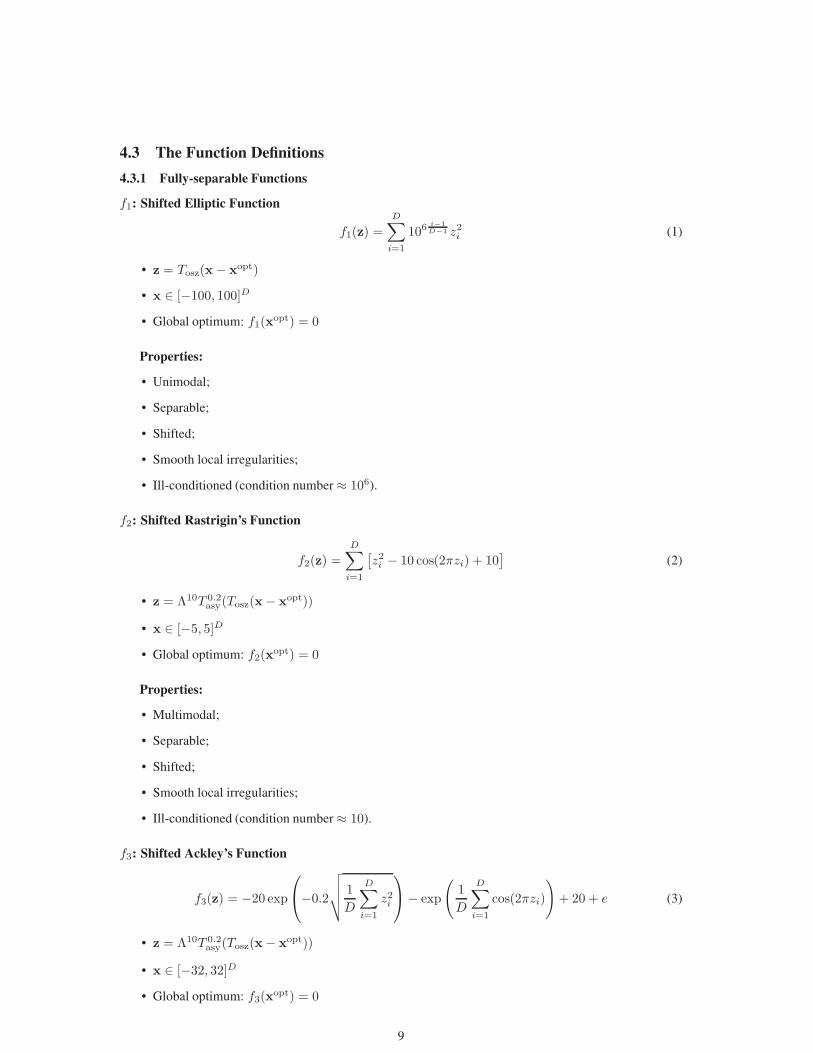
4.3 The Function Definitions

4.3.1 Fully-separable Functions

f1: Shifted Elliptic Function

f1(z) =

D∑

i=1

106i−1

D−1 z2i (1)

• z = Tosz(x− xopt)

• x ∈ [−100, 100]D

• Global optimum: f1(xopt) = 0

Properties:

• Unimodal;

• Separable;

• Shifted;

• Smooth local irregularities;

• Ill-conditioned (condition number ≈ 106).

f2: Shifted Rastrigin’s Function

f2(z) =

D∑

i=1

[

z2i − 10 cos(2πzi) + 10]

(2)

• z = Λ10T 0.2asy(Tosz(x− xopt))

• x ∈ [−5, 5]D


Properties:

• Multimodal;

• Separable;

• Shifted;



f3: Shifted Ackley’s Function

f3(z) = −20 exp

−0.2

√

√

√

√

1

D

D∑

i=1

z2i

− exp

(

1

D

D∑

i=1

cos(2πzi)

)

+ 20 + e (3)

• z = Λ10T 0.2asy(Tosz(x− xopt))

• x ∈ [−32, 32]D


9

Properties:

• Multimodal;

• Separable;

• Shifted;



10

4.3.2 Partially Additive Separable Functions I

f4: 7-nonseparable, 1-separable Shifted and Rotated Elliptic Function

f4(z) =

|S|−1∑

i=1

wifelliptic(zi) + felliptic(z|S|) (4)

• S = {50, 25, 25, 100, 50, 25, 25, 700}

• D =∑|S|

i=1 Si = 1000

• y = x− xopt

• yi = y(P[Ci−1+1] : P[Ci]), i ∈ {1, . . . , |S|}

• zi = Tosz(Riyi), i ∈ {1, . . . , |S| − 1}

• z|S| = Tosz(y|S|)

• Ri: a |Si| × |Si| rotation matrix

• x ∈ [−100, 100]D


Properties:

• Unimodal;

• Partially Separable;

• Shifted;



f5: 7-nonseparable, 1-separable Shifted and Rotated Rastrigin’s Function

f5(z) =

|S|−1∑

i=1

wifrastrigin(zi) + frastrigin(z|S|) (5)

• S = {50, 25, 25, 100, 50, 25, 25, 700}

• D =∑|S|

i=1 Si = 1000

• y = x− xopt

• yi = y(P[Ci−1+1] : P[Ci]), i ∈ {1, . . . , |S|}

• zi = Λ10T 0.2asy(Tosz(Riyi)), i ∈ {1, . . . , |S| − 1}

• z|S| = Λ10T 0.2asy(Tosz(y|S|))


• x ∈ [−5, 5]D


11

Properties:

• Multimodal;


• Shifted;



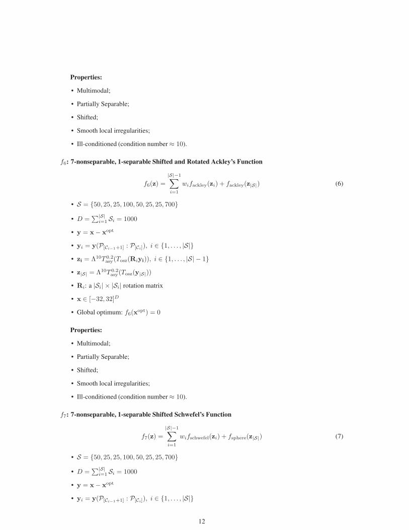
f6: 7-nonseparable, 1-separable Shifted and Rotated Ackley’s Function

f6(z) =

|S|−1∑

i=1

wifackley(zi) + fackley(z|S|) (6)

• S = {50, 25, 25, 100, 50, 25, 25, 700}

• D =∑|S|

i=1 Si = 1000

• y = x− xopt

• yi = y(P[Ci−1+1] : P[Ci]), i ∈ {1, . . . , |S|}

• zi = Λ10T 0.2asy(Tosz(Riyi)), i ∈ {1, . . . , |S| − 1}

• z|S| = Λ10T 0.2asy(Tosz(y|S|))


• x ∈ [−32, 32]D


Properties:

• Multimodal;


• Shifted;



f7: 7-nonseparable, 1-separable Shifted Schwefel’s Function

f7(z) =

|S|−1∑

i=1

wifschwefel(zi) + fsphere(z|S|) (7)

• S = {50, 25, 25, 100, 50, 25, 25, 700}

• D =∑|S|

i=1 Si = 1000

• y = x− xopt

• yi = y(P[Ci−1+1] : P[Ci]), i ∈ {1, . . . , |S|}

12

• zi = T 0.2asy(Tosz(Riyi)), i ∈ {1, . . . , |S| − 1}

• z|S| = T 0.2asy(Tosz(y|S|))


• x ∈ [−100, 100]D


Properties:

• Multimodal;


• Shifted;


13

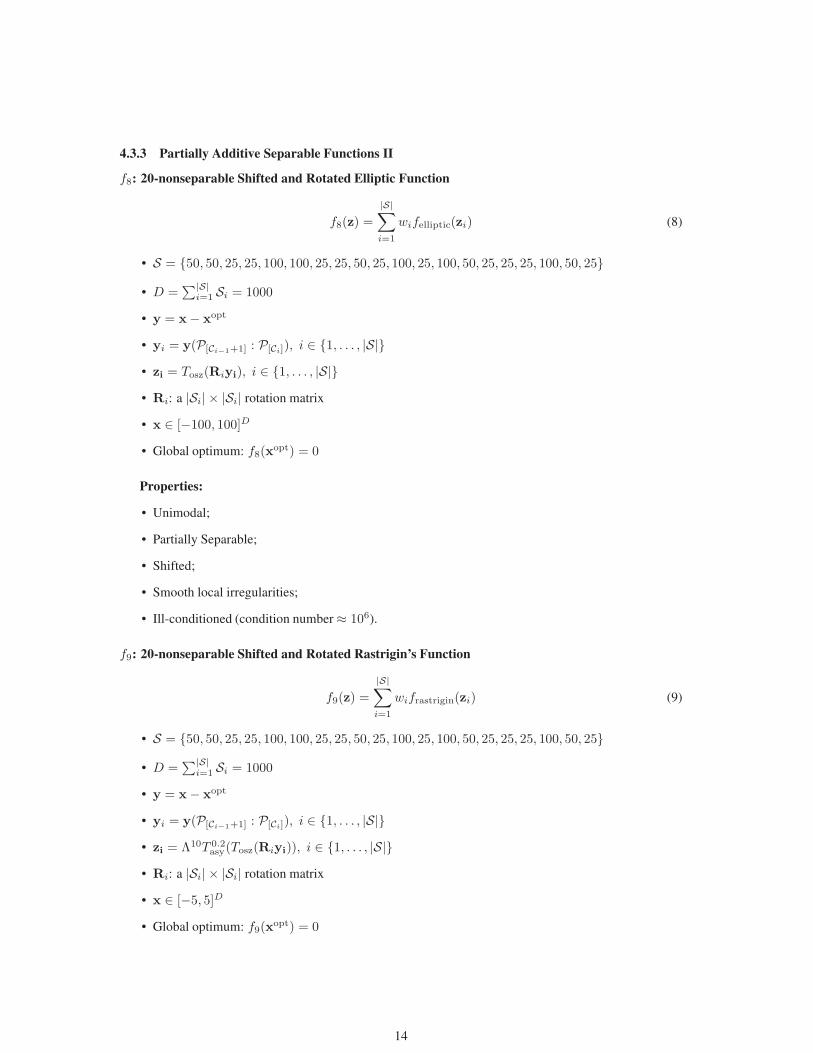
4.3.3 Partially Additive Separable Functions II

f8: 20-nonseparable Shifted and Rotated Elliptic Function

f8(z) =

|S|∑

i=1

wifelliptic(zi) (8)

• S = {50, 50, 25, 25, 100, 100, 25, 25, 50, 25, 100, 25, 100, 50, 25, 25, 25, 100, 50, 25}

• D =∑|S|

i=1 Si = 1000

• y = x− xopt

• yi = y(P[Ci−1+1] : P[Ci]), i ∈ {1, . . . , |S|}

• zi = Tosz(Riyi), i ∈ {1, . . . , |S|}


• x ∈ [−100, 100]D


Properties:

• Unimodal;


• Shifted;



f9: 20-nonseparable Shifted and Rotated Rastrigin’s Function

f9(z) =

|S|∑

i=1

wifrastrigin(zi) (9)

• S = {50, 50, 25, 25, 100, 100, 25, 25, 50, 25, 100, 25, 100, 50, 25, 25, 25, 100, 50, 25}

• D =∑|S|

i=1 Si = 1000

• y = x− xopt

• yi = y(P[Ci−1+1] : P[Ci]), i ∈ {1, . . . , |S|}

• zi = Λ10T 0.2asy(Tosz(Riyi)), i ∈ {1, . . . , |S|}


• x ∈ [−5, 5]D


14

Properties:

• Multimodal;

• Partially separable;

• Shifted;



f10: 20-nonseparable Shifted and Rotated Ackley’s Function

f10(z) =

|S|∑

i=1

wifackley(zi) (10)

• S = {50, 50, 25, 25, 100, 100, 25, 25, 50, 25, 100, 25, 100, 50, 25, 25, 25, 100, 50, 25}

• D =∑|S|

i=1 Si = 1000

• y = x− xopt

• yi = y(P[Ci−1+1] : P[Ci]), i ∈ {1, . . . , |S|}

• zi = Λ10T 0.2asy(Tosz(Riyi)), i ∈ {1, . . . , |S|}


• x ∈ [−32, 32]D


Properties:

• Multimodal;


• Shifted;



f11: 20-nonseparable Shifted Schwefel’s Function

f11(z) =

|S|∑

i=1

wifschwefel(zi) (11)

• S = {50, 50, 25, 25, 100, 100, 25, 25, 50, 25, 100, 25, 100, 50, 25, 25, 25, 100, 50, 25}

• D =∑|S|

i=1 Si = 1000

• y = x− xopt

• yi = y(P[Ci−1+1] : P[Ci]), i ∈ {1, . . . , |S|}

• zi = T 0.2asy(Tosz(Riyi)), i ∈ {1, . . . , |S|}


• x ∈ [−100, 100]D


15

Properties:

• Unimodal;


• Shifted;


16

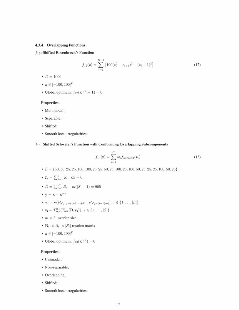
4.3.4 Overlapping Functions

f12: Shifted Rosenbrock’s Function

f12(z) =

D−1∑

i=1

[

100(z2i − zi+1)2 + (zi − 1)2

]

(12)

• D = 1000

• x ∈ [−100, 100]D

• Global optimum: f12(xopt + 1) = 0

Properties:

• Multimodal;

• Separable;

• Shifted;


f13: Shifted Schwefel’s Function with Conforming Overlapping Subcomponents

f13(z) =

|S|∑

i=1


• S = {50, 50, 25, 25, 100, 100, 25, 25, 50, 25, 100, 25, 100, 50, 25, 25, 25, 100, 50, 25}

• Ci =∑i

j=1 Si, C0 = 0

• D =∑|S|

i=1 Si −m(|S| − 1) = 905

• y = x− xopt

• yi = y(P[Ci−1−(i−1)m+1] : P[Ci−(i−1)m]), i ∈ {1, . . . , |S|}

• zi = T 0.2asy(Tosz(Riyi)), i ∈ {1, . . . , |S|}

• m = 5: overlap size


• x ∈ [−100, 100]D


Properties:

• Unimodal;

• Non-separable;

• Overlapping;

• Shifted;


17

f14: Shifted Schwefel’s Function with Conflicting Overlapping Subcomponents

f14(z) =

|S|∑

i=1


• S = {50, 50, 25, 25, 100, 100, 25, 25, 50, 25, 100, 25, 100, 50, 25, 25, 25, 100, 50, 25}

• D =∑|S|

i=1 Si − (m(|S| − 1)) = 905

• yi = x(P[Ci−1−(i−1)m+1] : P[Ci−(i−1)m])− xopti

• xopti : shift vector of size |Si| for the ith subcomponent

• zi = T 0.2asy(Tosz(Riyi))

• m = 5: overlap size


• x ∈ [−100, 100]D


Properties:

• Unimodal;

• Non-separable;

• Conflicting subcomponents;

• Shifted;


4.3.5 Fully Non-separable Functions

f15: Shifted Schwefel’s Function

f15(z) =D∑

i=1

i∑

j=1

xi

2

(15)

• D = 1000

• z = T 0.2asy(Tosz(x− xopt))

• x ∈ [−100, 100]D


Properties:

• Unimodal;

• Fully non-separable;

• Shifted;


18

5 Evaluation

5.1 General Settings

1. Problems: 15 minimization problems;

2. Dimensions: D = 1000;

3. Number of runs: 25 runs per function;

4. Maximum number of fitness evaluations: Max FE = 3× 106;

5. Termination criteria: when Max FE is reached.

6. Boundary Handling: All problems have the global optimum within the given bounds, so there is no

need to perform search outside of the given bounds for these problems. The provided codes returns

NaN if an objective function is evaluated outside the specified bounds.

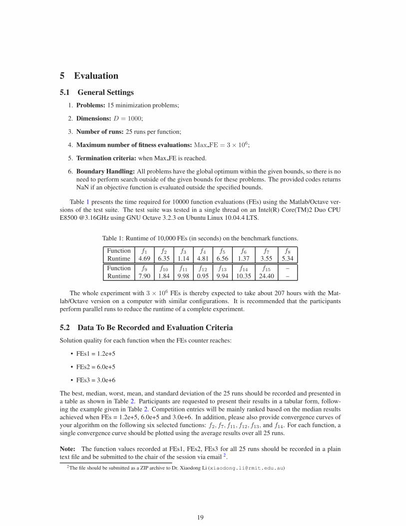
Table 1 presents the time required for 10000 function evaluations (FEs) using the Matlab/Octave ver-

sions of the test suite. The test suite was tested in a single thread on an Intel(R) Core(TM)2 Duo CPU

E8500 @3.16GHz using GNU Octave 3.2.3 on Ubuntu Linux 10.04.4 LTS.

Table 1: Runtime of 10,000 FEs (in seconds) on the benchmark functions.

Function f1 f2 f3 f4 f5 f6 f7 f8Runtime 4.69 6.35 1.14 4.81 6.56 1.37 3.55 5.34

Function f9 f10 f11 f12 f13 f14 f15 –

Runtime 7.90 1.84 9.98 0.95 9.94 10.35 24.40 –

The whole experiment with 3 × 106 FEs is thereby expected to take about 207 hours with the Mat-

lab/Octave version on a computer with similar configurations. It is recommended that the participants

perform parallel runs to reduce the runtime of a complete experiment.

5.2 Data To Be Recorded and Evaluation Criteria

Solution quality for each function when the FEs counter reaches:

• FEs1 = 1.2e+5

• FEs2 = 6.0e+5

• FEs3 = 3.0e+6

The best, median, worst, mean, and standard deviation of the 25 runs should be recorded and presented in

a table as shown in Table 2. Participants are requested to present their results in a tabular form, follow-

ing the example given in Table 2. Competition entries will be mainly ranked based on the median results

achieved when FEs = 1.2e+5, 6.0e+5 and 3.0e+6. In addition, please also provide convergence curves of

your algorithm on the following six selected functions: f2, f7, f11, f12, f13, and f14. For each function, a

single convergence curve should be plotted using the average results over all 25 runs.

Note: The function values recorded at FEs1, FEs2, FEs3 for all 25 runs should be recorded in a plain

text file and be submitted to the chair of the session via email 2.

2The file should be submitted as a ZIP archive to Dr. Xiaodong Li ([email protected])

19

[email protected]

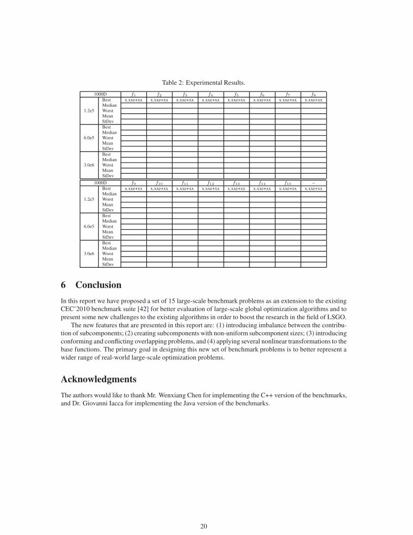
Table 2: Experimental Results.

1000D f1 f2 f3 f4 f5 f6 f7 f8Best x.xxe+xx x.xxe+xx x.xxe+xx x.xxe+xx x.xxe+xx x.xxe+xx x.xxe+xx x.xxe+xx

Median

1.2e5 Worst

Mean

StDev

Best

Median

6.0e5 Worst

Mean

StDev

Best

Median

3.0e6 Worst

Mean

StDev

1000D f9 f10 f11 f12 f13 f14 f15 –

Best x.xxe+xx x.xxe+xx x.xxe+xx x.xxe+xx x.xxe+xx x.xxe+xx x.xxe+xx x.xxe+xx

Median

1.2e5 Worst

Mean

StDev

Best

Median

6.0e5 Worst

Mean

StDev

Best

Median

3.0e6 Worst

Mean

StDev

6 Conclusion

In this report we have proposed a set of 15 large-scale benchmark problems as an extension to the existing

CEC’2010 benchmark suite [42] for better evaluation of large-scale global optimization algorithms and to

present some new challenges to the existing algorithms in order to boost the research in the field of LSGO.

The new features that are presented in this report are: (1) introducing imbalance between the contribu-

tion of subcomponents; (2) creating subcomponents with non-uniform subcomponent sizes; (3) introducing

conforming and conflicting overlapping problems, and (4) applying several nonlinear transformations to the

base functions. The primary goal in designing this new set of benchmark problems is to better represent a

wider range of real-world large-scale optimization problems.

Acknowledgments

The authors would like to thank Mr. Wenxiang Chen for implementing the C++ version of the benchmarks,

and Dr. Giovanni Iacca for implementing the Java version of the benchmarks.

20

References

[1] Thomas Back. Evolutionary Algorithms in Theory and Practice: Evolution Strategies, Evolutionary

Programming, Genetic Algorithms. ser. Dover Books on Mathematics. Oxford University Press, 1996.

[2] Thomas Back, David B Fogel, and Zbigniew Michalewicz, editors. Handbook of Evolutionary Com-

putation. Institute of Physics Publishing, Bristol, and Oxford University Press, New York, 1997.

[3] Richard E Bellman. Dynamic Programming. ser. Dover Books on Mathematics. Princeton University

Press, 1957.

[4] Wenxiang Chen, Thomas Weise, Zhenyu Yang, and Ke Tang. Large-scale global optimization using

cooperative coevolution with variable interaction learning. In Proc. of International Conference on

Parallel Problem Solving from Nature, volume 6239 of Lecture Notes in Computer Science, pages

300–309. Springer Berlin / Heidelberg, 2011.

[5] C. A. Coello Coello, D. A. Van Veldhuizen, and G. B. Lamont. Evolutionary Algorithms for Solving

Multi-Objective Problems. Kluwer Academic Publishers, New York, USA, 2002.

[6] George B. Dantzig and Philip Wolfe. Decomposition principle for linear programs. Operations

Research, 8(1):101–111, 1960.

[7] Yuval Davidor. Epistasis Variance: Suitability of a Representation to Genetic Algorithms. Complex

Systems, 4(4):369–383, 1990.

[8] Elizabeth D. Dolan, Jorge J. More, and Todd S. Munson. Benchmarking optimization software with

COPS 3.0. Technical report, Mathematics and Computer Science Division, Argonne National Labo-

ratory, 9700 South Cass Avenue, Argonne, Illinois 60439, 2004.

[9] Marco Dorigo, Vittorio Maniezzo, and Alberto Colorni. The Ant System: Optimization by a colony

of cooperating agents. IEEE Transactions on Systems, Man, and Cybernetics Part B: Cybernetics,

26(1):29–41, 1996.

[10] Fred W. Glover and Gary A. Kochenberger. Handbook of Metaheuristics. Springer, January 2003.

[11] A. Griewank and Ph. L. Toint. Local convergence analysis for partitioned quasi-newton updates.

Numerische Mathematik, 39:429–448, 1982. 10.1007/BF01407874.

[12] A. Griewank and Ph.L. Toint. Partitioned variable metric updates for large structured optimization

problems. Numerische Mathematik, 39:119–137, 1982.

[13] N. Hansen, S. Finck, R. Ros, and A. Auger. Real-parameter black-box optimization benchmarking

2009: Noiseless functions definitions. Technical Report RR-6829, INRIA, 2010.

[14] Martina Hasenjager, Bernhard Sendhoff, Toyotaka Sonoda, and Toshiyuki Arima. Three dimensional

evolutionary aerodynamic design optimization with CMA-ES. In Proc. of Genetic and Evolutionary

Computation Conference, pages 2173–2180, 2005.

[15] James Kennedy and Russell Eberhart. Particle swarm optimization. In Proc. of IEEE International

Conference on Neural Networks, volume 4, pages 1942–1948, 1995.

[16] S. Kirkpatrick, C.D. Gelatt, and M.P. Vecchi. Optimization by simulated annealing. Science Maga-

zine, 220(4598):671, 1983.

[17] P. Larraaga and J.A. Lozano. Estimation of Distribution Algorithms: A new tool for evolutionary

computation. Kluwer Academic Pub, 2002.

[18] Xiaodong Li and Xin Yao. Cooperatively coevolving particle swarms for large scale optimization.

IEEE Transactions on Evolutionary Computation, 16(2):210–224, April 2012.

21

[19] Y. Liu, X. Yao, Q. Zhao, and T. Higuchi. Scaling up fast evolutionary programming with cooperative

coevolution. In Proc. of IEEE Congress on Evolutionary Computation, pages 1101–1108, 2001.

[20] C.B. Lucasius and G. Kateman. Genetic algorithms for large-scale optimization in chemometrics: An

application. TrAC Trends in Analytical Chemistry, 10(8):254 – 261, 1991.

[21] Z. Michalewicz and David B. Fogel. How to solve It: Modern Heuristics. Springer, 2000.

[22] D. Molina, M. Lozano, and F. Herrera. MA-SW-Chains: Memetic algorithm based on local search

chains for large scale continuous global optimization. In Proc. of IEEE Congress on Evolutionary

Computation, pages 3153–3160, july 2010.

[23] P Moscato. On evolution, search, optimization, genetic algorithms and martial arts: Towards memetic

algorithms. Technical report, Caltech Concurrent Computation Program, 1989.

[24] Heinz Muhlenbein and Gerhard Paass. From recombination of genes to the estimation of distributions

i. binary parameters. In Proc. of International Conference on Parallel Problem Solving from Nature,

pages 178–187, London, UK, 1996. Springer-Verlag.

[25] M Olhofer, Y Jin, and B. Sendhoff. Adaptive encoding for aerodynamic shape optimization using

evolution strategies. In Proc. of IEEE Congress on Evolutionary Computation), volume 2, pages

576–583. IEEE Press, May 2001.

[26] Mohammad Nabi Omidvar, Xiaodong Li, Zhenyu Yang, and Xin Yao. Cooperative co-evolution for

large scale optimization through more frequent random grouping. In Proc. of IEEE Congress on

Evolutionary Computation, pages 1754–1761, 2010.

[27] Mohammad Nabi Omidvar, Xiaodong Li, and Xin Yao. Cooperative co-evolution with delta grouping

for large scale non-separable function optimization. In Proc. of IEEE Congress on Evolutionary

Computation, pages 1762–1769, 2010.

[28] Mohammad Nabi Omidvar, Xiaodong Li, and Xin Yao. Smart use of computational resources based

on contribution for cooperative co-evolutionary algorithms. In Proc. of Genetic and Evolutionary

Computation Conference, pages 1115–1122. ACM, 2011.

[29] Martin Pelikan and David E. Goldberg. BOA: The Bayesian Optimization Algorithm. In Proc. of

Genetic and Evolutionary Computation Conference, pages 525–532. Morgan Kaufmann, 1999.

[30] Martin Pelikan, David E. Goldberg, and Fernando G. Lobo. A survey of optimization by building and

using probabilistic models. Comp. Opt. and Appl., 21(1):5–20, 2002.

[31] Martin Pelikan, David E. Goldberg, and Shigeyoshi Tsutsui. Combining the strengths of bayesian

optimization algorithm and adaptive evolution strategies. In Proc. of Genetic and Evolutionary Com-

putation Conference, pages 512–519, San Francisco, CA, USA, 2002. Morgan Kaufmann Publishers

Inc.

[32] Martin Pelikan, Martin Pelikan, David E. Goldberg, and David E. Goldberg. Escaping hierarchical

traps with competent genetic algorithms. In Proc. of Genetic and Evolutionary Computation Confer-

ence, pages 511–518. Morgan Kaufmann, 2001.

[33] Ying ping Chen, Tian li Yu, Kumara Sastry, and David E. Goldberg. A survey of linkage learning

techniques in genetic and evolutionary algorithms. Technical report, Illinois Genetic Algorithms

Library, April 2007.

[34] Mitchell A. Potter and Kenneth A. De Jong. A cooperative coevolutionary approach to function opti-

mization. In Proc. of International Conference on Parallel Problem Solving from Nature, volume 2,

pages 249–257, 1994.

[35] K.V. Price, R.N. Storn, and J.A. Lampinen. Differential Evolution: A Practical Approach to Global

Optimization. Natural Computing Series. Springer, 2005.

22

[36] Ralf Salomon. Reevaluating genetic algorithm performance under coordinate rotation of benchmark

functions - a survey of some theoretical and practical aspects of genetic algorithms. BioSystems,

39:263–278, 1995.

[37] Yun-Wei Shang and Yu-Huang Qiu. A note on the extended rosenbrock function. Evolutionary

Computation, 14(1):119–126, March 2006.

[38] Jaroslaw Sobieszczanski-Sobieski and Raphael T. Haftka. Multidisciplinary aerospace design opti-

mization: Survey of recent developments. Structural Optimization, 14:1–23, August 1997.

[39] Rainer Storn and Kenneth Price. Differential evolution . a simple and efficient heuristic for global

optimization over continuous spaces. Journal of Global Optimization 11 (4), pages 341–359, 1995.

[40] P.N. Suganthan, N. Hansen, J.J. Liang, K. Deb, Y.P. Chen, A. Auger, and S. Tiwari. Problem defini-

tions and evaluation criteria for the cec 2005 special session on real-parameter optimization. Technical

report, Nanyang Technological University, Singapore, 2005. http://www.ntu.edu.sg/home/EPNSugan.

[41] K. Tang, X. Yao, P. N. Suganthan, C. MacNish, Y. P. Chen, C. M. Chen, , and Z. Yang. Bench-

mark functions for the CEC’2008 special session and competition on large scale global optimization.

Technical report, Nature Inspired Computation and Applications Laboratory, USTC, China, 2007.

http://nical.ustc.edu.cn/cec08ss.php.

[42] Ke Tang, Xiaodong Li, P. N. Suganthan, Zhenyu Yang, and Thomas Weise. Benchmark func-

tions for the CEC’2010 special session and competition on large-scale global optimization. Tech-

nical report, Nature Inspired Computation and Applications Laboratory, USTC, China, 2009.

http://nical.ustc.edu.cn/cec10ss.php.

[43] Philippe L. Toint. Test problems for partially separable optimization and results for the routine PSP-

MIN. Technical report, The University of Namur, Department of Mathematics, Belgium, 1983.

[44] F. van den Bergh and Andries P Engelbrecht. A cooperative approach to particle swarm optimization.

IEEE Transactions on Evolutionary Computation, 8(3):225–239, 2004.

[45] Thomas Weise, Raymond Chiong, and Ke Tang. Evolutionary Optimization: Pitfalls and Booby

Traps. Journal of Computer Science and Technology (JCST), 27(5):907–936, 2012. Special Issue on

Evolutionary Computation.

[46] Zhenyu Yang, Ke Tang, and Xin Yao. Large scale evolutionary optimization using cooperative co-

evolution. Information Sciences, 178:2986–2999, August 2008.

[47] Zhenyu Yang, Ke Tang, and Xin Yao. Multilevel cooperative coevolution for large scale optimization.

In Proc. of IEEE Congress on Evolutionary Computation, pages 1663–1670, June 2008.

23

benchmark functions for the cec’2013 special session and ...e46507/cec13-lsgo/... · (i.e. m =...

Documents