benchmarking big-data workflows across european academic

Bachelor’s Thesis

Benchmarking Big-Data WorkflowsAcross European Academic Clouds toEvaluate Cloud Bursting Strategies

Andreas Skorczyk

Examiner: Prof. Dr. Rolf BackofenAdvisers: Dr. Björn Grüning, Gianmauro Cuccuru

Albert-Ludwigs-University Freiburg

Faculty of Engineering

Department of Computer Science

Bioinformatics Group

September 10th, 2019

Writing Period

10. 06. 2019 – 10. 09. 2019

Examiner

Prof. Dr. Rolf Backofen

Advisers

Dr. Björn Grüning, Gianmauro Cuccuru

Declaration

I hereby declare, that I am the sole author and composer of my thesis and that no

other sources or learning aids, other than those listed, have been used. Furthermore,

I declare that I have acknowledged the work of others by providing detailed references

of said work.

I hereby also declare, that my Thesis has not been prepared for another examination

or assignment, either wholly or excerpts thereof.

Place, Date Signature

i

Abstract

The Galaxy-Project, a web platform for big-data biomedical research, needs a lot

of computational resources and cloud bursting, e.g. sending excess workloads to

the cloud, may be a solution in high-demand situations. But how do the various

academic clouds, spread across Europe, perform? May one be better suited than the

other for a specific workload? Does physical distance and connectivity between data

centers play a big enough role? What about the underlying infrastructure? Do they

make a difference, even if the actual instance size is the same? In this work, where I

benchmarked various academic clouds in Europe, I want to answer these questions

and even offer a framework for future benchmarks, as the need for benchmarking

more clouds in the future arise.

Deutsche Version:

Das Galaxy-Project, eine Web-Platform für Big-Data biomedizinische Forschung,

hat große Rechenleistungsanforderungen und "Cloud Bursting", d.h. überschüssige

Anfragen an die Cloud delegieren, könnte bei hoher Last eine Lösung sein. Aber wie

verhalten sich die verschiedenen wissenschaftlichen Clouds, die über ganz Europa

verteilt sind? Ist die eine Cloud für einen bestimmten Workload besser geeignet

als die andere? Spielt die räumliche Distanz oder die Verbindung zwischen den

Rechenzentren eine Rolle? Wie sieht es mit der Infrastrukutur aus? Gibt es hier

Unterschiede, auch wenn die tatsächliche Recheninstanz-Größe die gleiche ist? In

dieser Arbeit, in der ich verschiedene wissenschaftliche Clouds in Europa benchmarke,

möchte ich diese Fragen beantworten und eine Framework bieten, das bei zukünftigen

Benchmarks unterstützen kann.

iii

Contents

1 Introduction 1

2 Related Work 5

3 Background: Used tools and services 7

3.1 "The Cloud" . . . . . . . . . . . . . . . . . . . . . . . . . . . . . . . 7

3.1.1 OpenStack - Building Cloud Infrastructure . . . . . . . . . . 8

3.1.2 Terraform - Infrastructure as Code . . . . . . . . . . . . . . . 8

3.1.3 Ansible - Server Provisioning . . . . . . . . . . . . . . . . . . 9

3.2 Scientific Workbench . . . . . . . . . . . . . . . . . . . . . . . . . . . 9

3.2.1 Galaxy - Scientific Framework . . . . . . . . . . . . . . . . . . 9

3.2.2 Pulsar - Remote Job Runner . . . . . . . . . . . . . . . . . . 10

3.2.3 BioBlend - Python Library for Galaxy . . . . . . . . . . . . . 11

3.2.4 Planemo - CLI Tool for Galaxy . . . . . . . . . . . . . . . . . 12

3.2.5 Conda - Dependency and Environment Management . . . . . 12

3.3 Backend software . . . . . . . . . . . . . . . . . . . . . . . . . . . . . 12

3.3.1 RabbitMQ - Message Queue . . . . . . . . . . . . . . . . . . . 12

3.3.2 HTCondor - Job Scheduler . . . . . . . . . . . . . . . . . . . 13

3.4 Monitoring and Analytics . . . . . . . . . . . . . . . . . . . . . . . . 13

3.4.1 InfluxDB - Time Series Database . . . . . . . . . . . . . . . . 13

3.4.2 Telegraf - Collecting Metrics . . . . . . . . . . . . . . . . . . . 13

3.4.3 Grafana - Monitoring and Analytics . . . . . . . . . . . . . . 14

v

4 Approach 15

4.1 Goals . . . . . . . . . . . . . . . . . . . . . . . . . . . . . . . . . . . 15

4.2 Metrics . . . . . . . . . . . . . . . . . . . . . . . . . . . . . . . . . . 15

4.2.1 Staging Time . . . . . . . . . . . . . . . . . . . . . . . . . . . 16

4.2.2 CPU Time and Overall Runtime . . . . . . . . . . . . . . . . 16

4.3 Benchmark Types . . . . . . . . . . . . . . . . . . . . . . . . . . . . . 17

4.3.1 Destination Comparison . . . . . . . . . . . . . . . . . . . . . 17

4.3.2 Cold vs. Warm . . . . . . . . . . . . . . . . . . . . . . . . . . 18

4.3.3 Burst . . . . . . . . . . . . . . . . . . . . . . . . . . . . . . . 18

4.4 The Benchmarking Framework . . . . . . . . . . . . . . . . . . . . . 19

5 Results 21

5.1 Benchmarking Pulsar Locations across Europe . . . . . . . . . . . . . 21

5.1.1 Benchmarking Small, Short Running Workflows . . . . . . . . 23

5.1.2 Benchmarking Bigger, Long Running Workflows . . . . . . . 28

5.1.3 Benchmarking Workflows with many Files . . . . . . . . . . . 34

5.1.4 Benchmarking the Connection Speed of Destinations . . . . . 37

5.1.5 Conclusions of the Destination Comparison . . . . . . . . . . 39

5.2 Determining Staging Time on a Freshly Installed Pulsar Instance . . 42

5.2.1 Results . . . . . . . . . . . . . . . . . . . . . . . . . . . . . . 43

5.3 Stress Testing HTCondor Clusters . . . . . . . . . . . . . . . . . . . 45

5.3.1 Determining the Submit Rate . . . . . . . . . . . . . . . . . . 46

5.3.2 Performing the Stress Tests . . . . . . . . . . . . . . . . . . . 47

6 Conclusion 51

7 Acknowledgments 53

Bibliography 56

vi

List of Figures

1 Growth of UseGalaxy.eu, the biggest public Galaxy instance in Europe 1 1

2 Example of a Galaxy workflow . . . . . . . . . . . . . . . . . . . . . 10

3 The simplified communication between Galaxy and Pulsar using Rab-

bitMQ . . . . . . . . . . . . . . . . . . . . . . . . . . . . . . . . . . . 11

4 Flow of job stages over time . . . . . . . . . . . . . . . . . . . . . . . 16

5 Example configuration for the benchmarking framework . . . . . . . 19

6 Pulsar

Locations 2 . . . . . . . . . . . . . . . . . . . . . . . . . . . . . . . . 21

7 Results of the benchmarking

Total workflow runtime (left) and total staging time (right) of the

"HiC Explorer" workflow per destination. . . . . . . . . . . . . . . . 33

8 Results of the benchmarking

Total workflow runtime (left) and total staging time (right) by workflow

and destination. . . . . . . . . . . . . . . . . . . . . . . . . . . . . . 39

9 Simple test-job . . . . . . . . . . . . . . . . . . . . . . . . . . . . . . 45

vii

List of Tables

1 Pulsar Clusters in Europe that were benchmarked . . . . . . . . . . . 21

2 Workflows that were used for benchmarking . . . . . . . . . . . . . . 22

3 Total Workflow runtime of the Ard workflow . . . . . . . . . . . . . . 23

4 Sum of CPU time of the Ard workflow . . . . . . . . . . . . . . . . . 24

5 Dataset upload time of the Ard workflow . . . . . . . . . . . . . . . . 24

6 Tool installation time of the Ard workflow . . . . . . . . . . . . . . . 24

7 Sending results back time of the Ard workflow . . . . . . . . . . . . . 25

8 Median sum of staging times of the Ard workflow . . . . . . . . . . . 25

9 Total workflow runtime of the Adaboost workflow . . . . . . . . . . . 26

10 CPU time of the Adaboost workflow . . . . . . . . . . . . . . . . . . 26

11 Dataset upload time of the Adaboost workflow . . . . . . . . . . . . 26

12 Tool installation time of the Adaboost workflow . . . . . . . . . . . . 27

13 Sending results back time of the Adaboost workflow . . . . . . . . . 27

14 Median sum of staging times of the Adaboost workflow . . . . . . . . 27

15 Total workflow runtime of the "Mapping by Sequencing" workflow . 28

16 CPU time of the "Mapping by Sequencing" workflow . . . . . . . . . 29

17 Dataset upload time of the "Mapping by Sequencing" workflow . . . 29

18 Tool installation time of the "Mapping by Sequencing" workflow . . 29

19 Sending results back time of the "Mapping by Sequencing" workflow 30

20 Median sum of staging times of the "Mapping by Sequencing" workflow 30

21 Total workflow runtime of the "HiC Explorer" workflow . . . . . . . 32

ix

22 CPU time of the "HiC Explorer" workflow . . . . . . . . . . . . . . . 32

23 Dataset upload time of the "HiC Explorer" workflow . . . . . . . . . 32

24 Tool installation time of the "HiC Explorer" workflow . . . . . . . . 32

25 Sending results back time of the "HiC Explorer" workflow . . . . . . 33

26 Median sum of staging times of the "HiC Explorer" workflow . . . . 33

27 Total workflow runtime of the "Docking with Vina" workflow . . . . 34

28 CPU time of the "Docking with Vina" workflow . . . . . . . . . . . . 35

29 Dataset upload time of the "Docking with Vina" workflow . . . . . . 35

30 Tool installation time of the "Docking with Vina" workflow . . . . . 35

31 Sending results back time of the "Docking with Vina" workflow . . . 36

32 Median sum of staging times of the "Docking with Vina" workflow . 36

33 Total Workflow Runtime of the "Big File" workflow . . . . . . . . . . 37

34 CPU Time of the "Big File" workflow . . . . . . . . . . . . . . . . . 38

35 Dataset Upload Time (Galaxy → Pulsar) of the "Big File" workflow 38

36 Sending Results Back (Pulsar → Galaxy) of the "Big File" workflow 38

37 Approximate transfer speeds based on staging times of the "Big File"

workflow . . . . . . . . . . . . . . . . . . . . . . . . . . . . . . . . . . 39

38 Summary of the Destination Comparison . . . . . . . . . . . . . . . . 41

39 Instances used in Cold vs Warm Benchmark . . . . . . . . . . . . . . 42

40 Median total workflow runtimes of the Cold vs Warm benchmark . . 43

41 Median CPU time of the Cold vs Warm benchmark . . . . . . . . . . 43

42 Median Tool Installation Time of the Cold vs Warm benchmark . . . 43

43 Instances used in HTCondor stresstest . . . . . . . . . . . . . . . . . 45

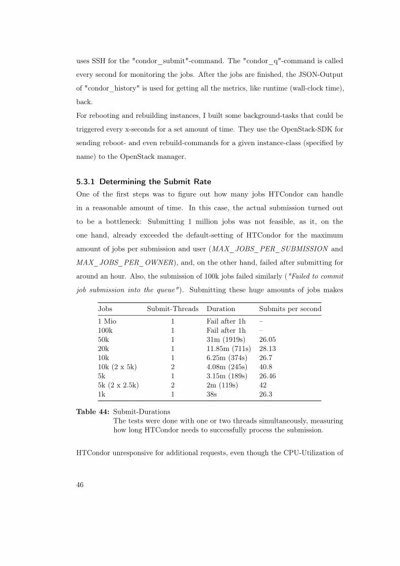
44 Submit-Durations

The tests were done with one or two threads simultaneously, measuring

how long HTCondor needs to successfully process the submission. . . 46

45 Results of the HTCondor Stresstest, which consisted of 10k jobs all

sleeping for one second . . . . . . . . . . . . . . . . . . . . . . . . . . 47

x

46 Results of the HTCondor Stresstest, which consisted of 10k jobs all

sleeping for one second . . . . . . . . . . . . . . . . . . . . . . . . . . 48

xi

1 Introduction

Figure 1: Growth of UseGalaxy.eu, the biggest public Galaxy instance in Europe 1

Galaxy is an open-source platform for scientific computations, used primarily in

data-intensive biomedical research. It offers a simple to use web-based user interface

for researchers to upload their data, select the tools, set their parameters, and simply

run the computations, without any programming knowledge needed. All the heavy

lifting, like managing infrastructure, allocating compute-resources, setting up tools,

etc. is done for them. Additionally, it enables reproducible results, as workflows can

easily be created, shared, and rerun at any point.

The platform has a modular design with the purpose of integrating easily into existing

infrastructure. For example, there are numerous ways (so-called "job-runners") for

Galaxy to submit a job to: Jobs can, among others, be just run on the local Galaxy

instance, processed on an HPC-Cluster, or run via Kubernetes. Moreover, Galaxy

can work with multiple options (also called "job-destinations") at the same time,

allowing jobs to be routed based on factors like the tool, the submitting user or other

conditions.1More statistics can be found at: https://stats.galaxyproject.eu/d/000000012/galaxy-user-statistics

1

UseGalaxy.eu, the biggest public Galaxy instance in Europe, currently runs all of its

computations in Freiburg, Germany and the de.NBI-Cloud. As the number of users

on UseGalaxy.eu and therefore the need for computational resources continuously

grows (Fig. 1), the idea of using a cloud bursting approach was considered. In this,

excess workloads are sent to "The Cloud", lowering the local processing needs. There

are a bunch of academic clouds in Europe that could be utilized for this purpose.

However, for the regular compute options, Galaxy needs a shared file system, which

is not always given and even becomes a problem for jobs that should be sent to a

different data center. For this use case, Pulsar was developed: It enables Galaxy

instances to submit jobs remotely without needing to share a file system with the

other location. Pulsar, which runs in the remote location, takes over some of the tasks

that Galaxy typically performs: It installs all the dependencies, submits the jobs to

its local cluster, collects the results after the computations have been completed and

sends them back to the Galaxy instance.

Pulsar, compared to the Galaxy Project itself, is not widely used yet, so the positive

and negative impacts of this integration need to be studied further. This means

finding out what types of workloads are suitable for outsourcing with Pulsar and

what the differences are between each cloud. The results of these tests might later

play a role in determining to which cloud a type of workload should best be routed

to. Factors that could contribute to the decision making might be the runtime of a

workflow or the utilization of a location in the sense to most efficiently utilize the

available resources. When considering using a public cloud, cost would be another

factor to keep in mind: What instance type is the most affordable one for a specific

workflow? Is it better to use a fast, expensive instance or could it be cheaper to

utilize a slower one, while also paying less per hour?

This work aims to build a general solution for benchmarking different Galaxy job-

destinations in a straightforward, reproducible, and extendable way. It primarily

focuses on benchmarking academic clouds that offer Pulsar, a server for executing

Galaxy jobs on a remote cluster, but the benchmarking framework that I built in

2

the process of this work can easily be extended to cover more options in the future.

The framework later is used to run various real-life workflows, that have different

characteristics in terms of resource usages, on several academic clouds to see if there

are significant performance differences depending on the workload. The results of this

work may help UseGalaxy.eu to determine which workloads are suitable for cloud

bursting and which cloud a specific workload should be best routed to.

3

2 Related Work

The term "benchmarking" has a broad definition and has been in use for a long

time already. In its basic form, it refers to the process of evaluating a subject using

some metrics to determine its performance in comparison to others. In the business

sector, for example, this can mean analyzing the own cost of production for a product

compared to the competition. In the case of this work and also in the more broad

sense of the IT sector, benchmarking is concerned about comparing and evaluating

components or even whole systems to one another using some specific metrics. As

a simple example, that could mean, measuring and comparing the runtime for the

same tool and data on different hardware, or study the behavior, like latency or

throughput, of a system in high load.

Benchmarking the cloud is still a relatively new sector on its own. Up to now,

the components and conditions of a subject to benchmark were mostly well known.

However, today an auditor might not even know what infrastructure really lies

behind a cloud offering - it is more or less a black box. This is, of course, true for

"Software as a Service" (SaaS) offerings like a managed database, but even if an

auditor controls the software, the underlying hardware is often hidden. At the same

time, the infrastructure, that for, examples, runs a compute instance, can be shared

with other users, which may lead to a varying performance depending on different

factors, making the general conditions for benchmarking more difficult [1].

Now, benchmarking Galaxy job-destinations even is a completely new sector. To the

best of my knowledge, there is currently no solution for benchmarking Galaxy or a

5

comprehensive test for comparing different job-destinations. So in the beginning, it

was not clear what the best strategy would be for a benchmark, what metrics to look

at and how to even perform such a test. For that reason, I could not build much

on previous work but had to develop a whole framework more or less from scratch.

However, the basic principles for building a solid benchmark still apply.

6

3 Background: Used tools and services

There are a lot of tools and services involved in performing a benchmark. First of all,

the underlying infrastructure needs to be built and managed, meaning starting all the

necessary instances and configuring them correctly in the cloud. The Galaxy instance

itself needs to be deployed and provisioned properly to work with the benchmarking

framework. Later, requirements for workflows have to be met and they need to be

scheduled somehow. And in the end, the resulting metrics need to be gathered, stored,

processed and visualized to make the most out of them. The following is a summary

with some short explanations for each software and service that was used in the

process of this work. For a more elaborate description, I refer to each projects site.

3.1 "The Cloud"

The term "cloud" today is used in a broad sense describing many different types of

services. In essence, it is about the usage of infrastructure (like compute or storage

resources) and services (like managed databases or DNS servers, but also end-user

faced applications like online text editing) on an on-demand basis, mostly as a self-

service offering. Additionally, cloud offerings can be divided into two kinds: public

and private clouds. Providers like Amazon Web Services (AWS), Google Cloud, or

Microsoft Azure can be ranged into this category. Essentially, this type is available to

the public and can be used by everyone. In most cases, it is priced on a pay-as-you-use

basis, only paying for the resources that are actually needed, which makes it very

7

flexible. On the other hand, a private cloud is run and managed by an institution

with its own data centers and only meant to be offered to its internal users. The

academic clouds benchmarked in this work can be classified into this latter category,

as they are run by different universities and not meant to be available to the general

public.

In cloud computing, users typically share the underlying hardware, which means that

a virtual CPU (vCPU) of an instance might not necessarily map to one physical CPU

core that is reserved for one user only. Overbooking is a common thing, meaning a

provider offers more vCPUs than physically available. If balanced properly, this does

not necessarily mean a problem, as not every user typically runs its instance at 100

percent utilization all the time. However, if it is, on purpose or not, off-balanced, it

can lead to lower or varying performance depending on factors like the time of day.

3.1.1 OpenStack - Building Cloud Infrastructure

OpenStack is an open-source platform for building a cloud infrastructure, similar to

services offered by AWS, Azure or Google Cloud. It lets data center operators offer

their users a self-service platform for compute, storage, and other resources with a

common web-interface, CLI, and API across all operators [2].

OpenStack is the de facto standard for the academic clouds, which is also used on

clouds that I benchmarked in this work.

3.1.2 Terraform - Infrastructure as Code

The idea behind Terraform 1 is to define Infrastructure as Code (IaC), describing it

in a high-level configuration syntax. "Infrastructure" in this sense can mean low-level

components like compute instances or storage, but also high-level components like

DNS entries. Terraform can be used for building a simple application, but also to

describe a whole data center. The advantage of this approach is the ability to use

existing version control systems for the description of the infrastructure. In that

way, the process of building the infrastructure can become similar to shipping regular1https://www.terraform.io/intro/index.html

8

software. Also, Terraform is able to work with a variety of different cloud providers

like Google Cloud, AWS or OpenStack using the same "language", allowing it to

combine multiple providers, but also to quickly move from one to the other if wanted

[3].

Terraform, in our case, is used for spinning up the VMs that are needed for the

benchmarking on the OpenStack Clouds.

3.1.3 Ansible - Server Provisioning

Ansible is a provisioning tool that enables consistent configuration of machines. One

of the differences compared to other tools like Puppet is that it is agentless, e.g.,

there is no need to pre-install additional tools, as Ansible uses SSH for configuring a

machine.

A configuration is defined in states that a system should be in, like a folder should

exist with the given user mode, a configuration file should contain this line, a service

should be running, a software tool should be installed in the following version, etc.

Ansible will make sure that the state is met by SSH-ing into the system, evaluating the

current state and running the needed commands to get the system to the appropriate

condition [4].

In our case, Ansible is used for configuring the VMs and services, while the bench-

marking framework also makes use of Ansible for automatically configuring Galaxy to

use various job-destinations, cleaning up servers or sending needed files to a server.

3.2 Scientific Workbench

3.2.1 Galaxy - Scientific Framework

Galaxy is a platform for data-intensive scientific computations, primarily used via a

web-interface. It is built with Python and is highly extendable in various ways.

The usage of Galaxy is based around community-developed tools, that can process

and work on all kinds of data, not limited to biomedical research only. Those tools

9

Figure 2: Example of a Galaxy workflowWorkflows can be edited inside the browser (left) and run after defining parameters and inputs (right).

process the given data with user-defined parameters and can be combined into work-

flows - a series of tools that further process the inputs (Fig. 2). An administrator

can customize Galaxy to its needs by installing all the necessary tools via an open

repository, called the "ToolShed" [5].

Galaxy can use various compute-options, ranging from just running it locally on

the same instance, to using containers with Kubernetes, to scheduling jobs to a

DRM-System, like HTCondor. However, in all of these cases, it expects a shared file

system, which can be problematic when trying to use a remote compute location.

That’s where Pulsar comes in.

3.2.2 Pulsar - Remote Job RunnerPulsar is a server written in Python that allows Galaxy instances to execute jobs

remotely without the need to have a shared file system. A Galaxy instance sends all

the data necessary to execute a job to Pulsar which handles the part of installing

and preparing all the tools (also called "staging"), scheduling the jobs, etc. After the

computations have been completed, the results are sent back to Galaxy.

10

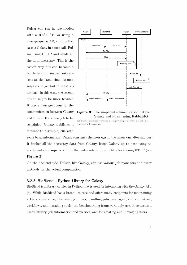
Figure 3: The simplified communication betweenGalaxy and Pulsar using RabbitMQ

Solid horizontal lines represent messages being sent, while dashed lines

represent a file transfer.

Pulsar can run in two modes:

with a REST-API or using a

message queue (MQ). In the first

case, a Galaxy instance calls Pul-

sar using HTTP and sends all

the data necessary. This is the

easiest way but can become a

bottleneck if many requests are

sent at the same time, as mes-

sages could get lost in those sit-

uations. In this case, the second

option might be more feasible.

It uses a message queue for the

communication between Galaxy

and Pulsar: For a new job to be

scheduled, Galaxy publishes a

message to a setup-queue with

some basic information. Pulsar consumes the messages in the queue one after another.

It fetches all the necessary data from Galaxy, keeps Galaxy up to date using an

additional status-queue and at the end sends the result files back using HTTP (see

Figure 3).

On the backend side, Pulsar, like Galaxy, can use various job-managers and other

methods for the actual computation.

3.2.3 BioBlend - Python Library for GalaxyBioBlend is a library written in Python that is used for interacting with the Galaxy API

[6]. While BioBlend has a broad use case and offers many endpoints for maintaining

a Galaxy instance, like, among others, handling jobs, managing and submitting

workflows, and installing tools, the benchmarking framework only uses it to access a

user’s history, job information and metrics, and for creating and managing users.

11

3.2.4 Planemo - CLI Tool for Galaxy

Planemo is a command-line utility that assists in writing tools and workflows for

Galaxy, testing and deploying them [7]. Its functionality for testing workflows is used

in the benchmarking framework for submitting workflows and making sure that the

results of a workflow run are as expected. In the background, it uses BioBlend for

the interaction with Galaxy. Hence, my framework actually uses some additional

functionalities of BioBlend indirectly.

3.2.5 Conda - Dependency and Environment Management

Conda is an open-source system for managing packages and environments. It allows

to install specific virtual environments with the necessary dependencies that a tool

might need. In that way, various environments with different and possibly even

mutually exclusive dependencies can coexist on one machine, without interfering with

each other. Conda works for any language, not limited to Python [8]. It is used in

Galaxy and Pulsar to prepare virtual environments for each used tool and installing

the necessary dependencies.

3.3 Backend software

3.3.1 RabbitMQ - Message Queue

RabbitMQ is a message-broker software that implements AMQP, the Advanced

Message Queuing Protocol. It offers a central place for distributing messages (like

a job submit) between a sender and a receiver, which allows the two sides to be

decoupled from one another [9]. In this way, both can work "at their own pace"

without the need to wait for each other. The message-broker handles the routing

and delivery of the messages while beeing able to guarantee that a message will be

handled at some point, even if the receiver is currently busy or unavailable. In our

case, RabbitMQ is used for the communication between Galaxy and Pulsar.

12

3.3.2 HTCondor - Job Scheduler

HTCondor is a batch job management software that allows the distribution of jobs

around a pool of compute-resources [10]. It handles, among other things, the queuing

and scheduling of jobs, while factoring into the decision their resource-requirements

in terms of CPU cores, memory, or others.

3.4 Monitoring and Analytics

3.4.1 InfluxDB - Time Series Database

InfluxDB is a database that is optimized for storing and analyzing time-series data.

One of the key differences compared to a relational database is, that it does not

require defining database schemas upfront. Rather it is based around points in time,

that have "measurements" (for example CPU or Memory usage), at least one "value"

and zero to many "tags" that define the metadata (like a hostname). This property

makes it easy to collect lots of metrics and analyze them later, without having to

define much at the beginning [11]. InfluxDB is used for storing all the metrics that

are collected while benchmarking.

3.4.2 Telegraf - Collecting Metrics

elegraf is used to collect metrics and sending them to an InfluxDB instance. It runs

as an agent on the machine and is plugin-driven, which means, an operator can easily

extend its usage above basic metrics like CPU utilization or network I/O [12]. For

example, UseGalaxy.eu uses a plugin to monitor the queue size of its HTCondor

cluster.

Telegraf runs on the infrastructure used for my benchmarking, allowing the monitoring

of it and giving the ability to identify problems early on.

13

3.4.3 Grafana - Monitoring and AnalyticsGrafana helps to visualize all kinds of time-series data, coming from various sources

like InfluxDB, AWS Cloudwatch, Elasticsearch, and others. It offers a web-interface

for querying those data sources and also plot the underlying data in many ways [13].

Grafana is used to analyze and visualize the metrics coming from the benchmarking

framework.

14

4 Approach

At the beginning of this work, we asked ourselves what the goals of this benchmarking

are, what type of workloads should be used, and what metrics could be meaningful.

4.1 Goals

The most important aim of this work was to use workloads that are as close to reality

as possible. Of course, in some situations, it might make sense to measure the perfor-

mance of just one part of a system, like the read and write speed of the underlying

storage system, but in the case of the Galaxy-Project, many factors might play a role

in the overall performance of a workflow. Also, the underlying characteristics of two

distinct workflows can be completely different in areas like memory usage, I/O, or

CPU needs. So from the beginning, it was clear that Galaxy Workflows would be

used that are in production traffic too.

4.2 Metrics

As the main aim of this work was on comparing destinations across Europe, the focus

laid on the metrics of the staging time, the CPU time, and the runtime, both in

terms of overall runtime per workflow run, but also runtime per tool.

15

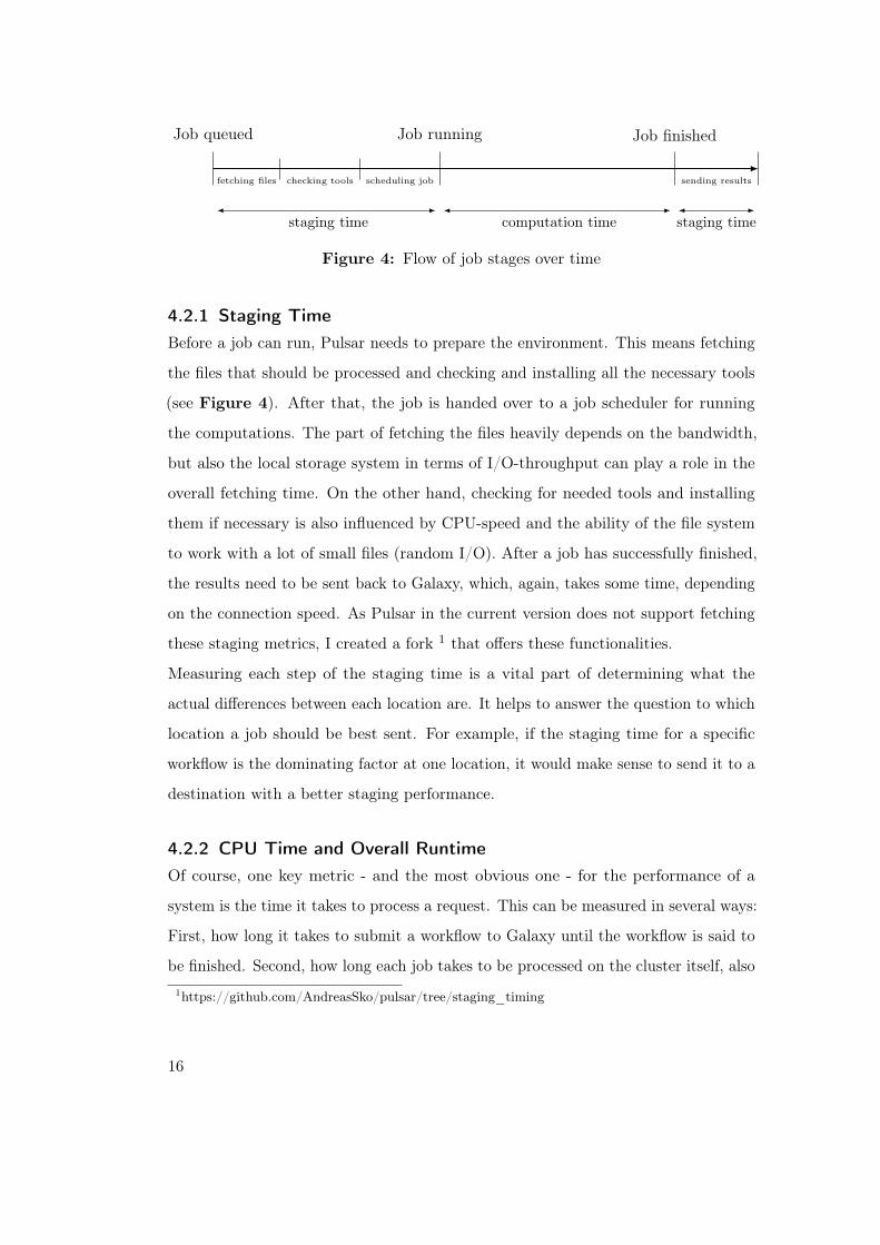
Job queued Job running

staging time computation time

fetching files checking tools scheduling job

Job finished

sending results

staging time

Figure 4: Flow of job stages over time

4.2.1 Staging TimeBefore a job can run, Pulsar needs to prepare the environment. This means fetching

the files that should be processed and checking and installing all the necessary tools

(see Figure 4). After that, the job is handed over to a job scheduler for running

the computations. The part of fetching the files heavily depends on the bandwidth,

but also the local storage system in terms of I/O-throughput can play a role in the

overall fetching time. On the other hand, checking for needed tools and installing

them if necessary is also influenced by CPU-speed and the ability of the file system

to work with a lot of small files (random I/O). After a job has successfully finished,

the results need to be sent back to Galaxy, which, again, takes some time, depending

on the connection speed. As Pulsar in the current version does not support fetching

these staging metrics, I created a fork 1 that offers these functionalities.

Measuring each step of the staging time is a vital part of determining what the

actual differences between each location are. It helps to answer the question to which

location a job should be best sent. For example, if the staging time for a specific

workflow is the dominating factor at one location, it would make sense to send it to a

destination with a better staging performance.

4.2.2 CPU Time and Overall RuntimeOf course, one key metric - and the most obvious one - for the performance of a

system is the time it takes to process a request. This can be measured in several ways:

First, how long it takes to submit a workflow to Galaxy until the workflow is said to

be finished. Second, how long each job takes to be processed on the cluster itself, also1https://github.com/AndreasSko/pulsar/tree/staging_timing

16

called wall-clock time. And third, what the CPU time for each job is, e.g., how long

each CPU core worked on the task. Combining these metrics with information about

the workflow, like how many CPU cores are used or if the workload is more CPU- or

I/O-bound, allows to make assumptions about the performance of the vCPUs and

the file system of a destination.

4.3 Benchmark Types

There are different scenarios that can be considered. For this, three benchmark types

were defined.

4.3.1 Destination ComparisonIn the destination comparison benchmark, the same workflows are run on multiple

destinations to see how each one performs compared to the others. There are several

possible ways, in which destinations can differ:

Underlying Infrastructure

Most of the time, the computing clusters will be different at each location. This

can be in the sense of the number of instances, vCPUs, or available RAM. But even

if these are the same, the underlying infrastructure of the virtual machines may

differ: different CPU vendors or versions, storage-systems, internet connectivity, and

even overbooking may play a role. All of these factors can influence the overall

performance.

Used Technologies

Pulsar enables the use of various options to run the computations. That means it

can, on the one hand, use different technologies to encapsulate the requirements like

Conda or Singularity, but also schedule and run the actual computations in many

ways (DRM-System like HTCondor or even Kubernetes). It is interesting to see

whether there are notable differences between the options, in resource-usage (like

17

memory), but also overall runtime, especially staging time. The results may help

determine what options are best for which use case.

Geographic Location

Transferring big datasets takes time. This is especially true if the computation is

not running locally but in a remote data center. Overhead may vary depending on

the physical connection between locations, the current load on the network or the

characteristics of the input - a lot of small files may take longer to transfer than a

few big ones. Figuring out what the actual overhead looks like may help to decide

in future, what kind of workloads make sens to be sent to a remote location and in

what situation it is more efficient to process it locally.

4.3.2 Cold vs. Warm

A service might perform different depending on it being used for the first time ("cold

run") versus already having performed a task multiple times ("warm run"). In the

second case, caching and already installed tools might play a role in faster execution

of a job, while a "cold" service may still need to bootstrap some tools. Therefore, it

may help to know what the usual time difference between a cold run and a warm run is.

4.3.3 Burst

Another possible scenario to look at is a traffic burst, e.g., many requests that need

to be handled at the same time. One might be interested in determining at what

point (requests per second or size of job queue) the performance starts to decrease

significantly and therefore what instance size (in terms of CPU count and available

memory) might be appropriate for production traffic.

18

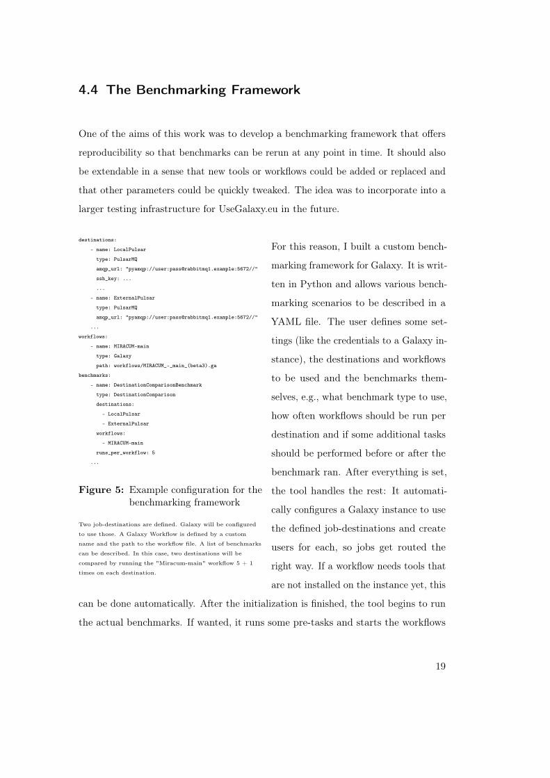
4.4 The Benchmarking Framework

One of the aims of this work was to develop a benchmarking framework that offers

reproducibility so that benchmarks can be rerun at any point in time. It should also

be extendable in a sense that new tools or workflows could be added or replaced and

that other parameters could be quickly tweaked. The idea was to incorporate into a

larger testing infrastructure for UseGalaxy.eu in the future.

destinations:

- name: LocalPulsar

type: PulsarMQ

amqp_url: "pyamqp://user:[email protected]:5672//"

ssh_key: ...

...

- name: ExternalPulsar

type: PulsarMQ

amqp_url: "pyamqp://user:[email protected]:5672//"

...

workflows:

- name: MIRACUM-main

type: Galaxy

path: workflows/MIRACUM_-_main_(beta3).ga

benchmarks:

- name: DestinationComparisonBenchmark

type: DestinationComparison

destinations:

- LocalPulsar

- ExternalPulsar

workflows:

- MIRACUM-main

runs_per_workflow: 5

...

Figure 5: Example configuration for thebenchmarking framework

Two job-destinations are defined. Galaxy will be configured

to use those. A Galaxy Workflow is defined by a custom

name and the path to the workflow file. A list of benchmarks

can be described. In this case, two destinations will be

compared by running the "Miracum-main" workflow 5 + 1

times on each destination.

For this reason, I built a custom bench-

marking framework for Galaxy. It is writ-

ten in Python and allows various bench-

marking scenarios to be described in a

YAML file. The user defines some set-

tings (like the credentials to a Galaxy in-

stance), the destinations and workflows

to be used and the benchmarks them-

selves, e.g., what benchmark type to use,

how often workflows should be run per

destination and if some additional tasks

should be performed before or after the

benchmark ran. After everything is set,

the tool handles the rest: It automati-

cally configures a Galaxy instance to use

the defined job-destinations and create

users for each, so jobs get routed the

right way. If a workflow needs tools that

are not installed on the instance yet, this

can be done automatically. After the initialization is finished, the tool begins to run

the actual benchmarks. If wanted, it runs some pre-tasks and starts the workflows

19

once without considering its metrics in the results to warmup the services. This

makes sure that metrics won’t get skewed by dependency resolution in case of a first

run. The workflows now run for the defined number of times. The metrics of the jobs

are collected after each run and saved in memory. When all the runs are finished, the

results are sent to InfluxDB for further analysis with Grafana.

The benchmarking framework supports the definition of tasks, that can be run before

or after a benchmark. It even allows to run these tasks periodically in the background.

Right now, these tasks can consist of an Ansible playbook file that should get run on

the destination, or a custom "BenchmarkerTask" that can be defined as a Python

function. These tasks could be used to, for example, install additional dependencies

or clean up a destination afterwards. Another use case is to define a function that

calls the OpenStack SDK to change the infrastructure while benchmarking.

In distributed systems, it is common to have a certain amount of arbitrarily failed

requests. The benchmarking framework is able to handle those failures by retrying

using a backoff strategy, skipping workflows if they fail a certain number of times for

a specific destination. This allows to move on with the benchmarking, without the

immediate need for intervention by the user.

The GalaxyBenchmarker 2 is written in a modular way, allowing it to be extended

for more benchmarking types or job-destinations in the future.

2The GalaxyBenchmarker can be found in my Github-Repository:https://github.com/AndreasSko/Galaxy-Benchmarker

20

5 Results

5.1 Benchmarking Pulsar Locations across Europe

Figure 6: PulsarLocations 1

For my work, I had the opportunity to benchmark sev-

eral clouds in Europe. The locations were in the cities

of Freiburg and Tübingen (both Germany), Bari (Italy),

Gent (Belgium), Lisbon (Portugal), and Didcot (United

Kingdom). All ran on Pulsar version 0.11.0, with Rab-

bitMQ as the message queue and HTCondor. The Galaxy

instance used for the benchmarking offers 16 vCPUs with

32GB RAM (m.xxlarge flavor) and is located in Freiburg.

As UseGalaxy.eu is hosted in the same data center, the

following results are realistic for this location. For other

regions, the results, especially the staging times, could

vary.

Location Worker Size # Worker Sponsor

Freiburg (Germany) 10 vCPUs, 55 GB RAM 2 BW CloudTübingen (Germany) 16 vCPUs, 32 GB RAM 3 de.NBIBari (Italy) 16 vCPUs, 32 GB RAM 5 INFN ReCaS-BariGent (Belgium) 8 vCPUs, 16 GB RAM 3 VIB, Center for Plant Systems

BiologyLisbon (Portugal) 4 vCPUs, 16 GB RAM 2 University of LisboaDidcot (United Kingdom) 60 vCPUs, 384GB RAM 2 Diamond Light Source

Table 1: Pulsar Clusters in Europe that were benchmarkedThanks to all providers of the infrastructure and the ELIXIR network!

1Image sources: "Pin" by Gregor Cresnar and "European Union" by Sergey Demushkin from theNoun Project

21

The following Workflows were used for benchmarking:

Workflow # Inputs Input sizes Output size Ø runtime

Adaboost 1 < 1kB 13kB 20sArd 1 < 1kB 3kB 20s

Docking with Vina 50 50 x 2kB = 100kB 50 x 2kB = 100kB 2-7m

Big File 1 1GB 1GB 10s

Mapping by Sequencing 3 60MB-120MB, Σ = 282MB 750MB 13-18mHiC Explorer 6 15MB - 550 MB, Σ = 1GB 10GB 2-5h

Table 2: Workflows that were used for benchmarking

Each tool within the workflows had one core available, making the comparison across

clusters with varying numbers of available vCPUs easier. I characterized the workflows

into five possible categories depending on their characteristics in the size of the input

data and the number of input files, and the total runtime:

a) Small input, few files, short runtime

b) Small input, many files, short runtime

c) Small input, long runtime

d) Big input, short runtime

e) Big input, long runtime

However, due to problems with Pulsar and Conda, I could not add a workflow that

would have been suitable for c).

If not stated otherwise, each workflow ran 1 + 15 times per destination, while the first

run per workflow and destination was not considered, as it may be skewed because

of dependency resolution and installation. The following duration values are in the

format of hours:minutes:seconds. I mainly focused on the median values, as it is

common in distributed systems to see some random spikes in the data, which can

22

skew mean values. To still notice values that might regularly fluctuate - which can

also be a quality sign in the negative sense -, I added the standard-deviation (stddev)

as a measure, together with the minimum and maximum values. Some values in the

tables are highlighted by color, representing outstanding ( green ), less than optimal

( yellow ), or bad ( red ) results. Those highlighted values are typically mentioned in

the discussion of each benchmark.

5.1.1 Benchmarking Small, Short Running Workflows

For this benchmark, I used Adaboost and Ard as they have similar characteristics in

terms of input size and overall runtime.

Ard Workflow

Description: Used in the machine learning area for comparing, validating, and

choosing parameters and models [14].

Characteristics: Low I/O, High CPU

Destination min max median mean stddev

United Kingdom 0:00:40 0:00:43 0:00:42 0:00:41 0:00:00Tübingen 0:00:43 0:00:45 0:00:44 0:00:44 0:00:00Portugal 0:00:56 0:01:08 0:01:00 0:01:01 0:00:03Freiburg 0:01:00 0:01:14 0:01:02 0:01:02 0:00:03Italy 0:01:11 0:01:42 0:01:19 0:01:20 0:00:07

Belgium 0:01:19 0:01:35 0:01:28 0:01:27 0:00:04Average: 0:01:03

Table 3: Total Workflow runtime of the Ard workflow

23

Destination median stddev

United Kingdom 0:00:04 0:00:00Tübingen 0:00:10 0:00:00Belgium 0:00:14 0:00:00Portugal 0:00:17 0:00:00Freiburg 0:00:23 0:00:00Italy 0:00:27 0:00:00

Average: 0:00:16

Table 4: Sum of CPU time of the Ard workflow


Freiburg 0:00:00 0:00:00 0:00:00 0:00:00 0:00:00Tübingen 0:00:00 0:00:00 0:00:00 0:00:00 0:00:00

United Kingdom 0:00:00 0:00:01 0:00:00 0:00:00 0:00:00Portugal 0:00:00 0:00:03 0:00:00 0:00:01 0:00:00Italy 0:00:00 0:00:03 0:00:00 0:00:01 0:00:00

Belgium 0:00:03 0:00:05 0:00:03 0:00:03 0:00:00Average: 0:00:01

Table 5: Dataset upload time of the Ard workflow


Freiburg 0:00:00 0:00:00 0:00:00 0:00:00 0:00:00Tübingen 0:00:00 0:00:00 0:00:00 0:00:00 0:00:00Portugal 0:00:00 0:00:00 0:00:00 0:00:00 0:00:00

United Kingdom 0:00:00 0:00:00 0:00:00 0:00:00 0:00:00Italy 0:00:00 0:00:01 0:00:00 0:00:00 0:00:00

Belgium 0:00:01 0:00:02 0:00:02 0:00:01 0:00:00Average: 0:00:00

Table 6: Tool installation time of the Ard workflow

24



United Kingdom 0:00:00 0:00:01 0:00:00 0:00:00 0:00:00Belgium 0:00:00 0:00:01 0:00:00 0:00:00 0:00:00Italy 0:00:00 0:00:00 0:00:00 0:00:00 0:00:00

Portugal 0:00:00 0:00:01 0:00:00 0:00:00 0:00:00Average: 0:00:00

Table 7: Sending results back time of the Ard workflow

Destination median

Freiburg 0:00:00Tübingen 0:00:00

United Kingdom 0:00:00Italy 0:00:00

Portugal 0:00:00Belgium 0:00:05Average: 0:00:01

Table 8: Median sum of staging times of the Ard workflow

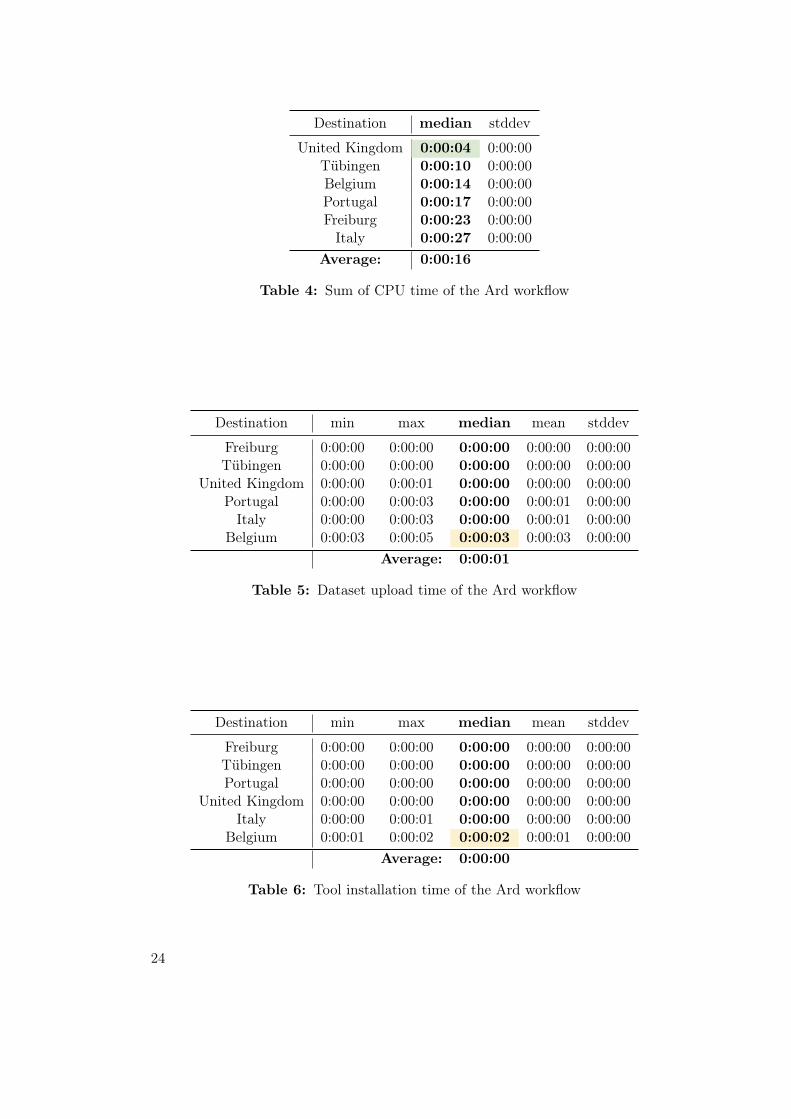
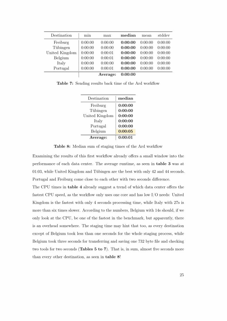
Examining the results of this first workflow already offers a small window into the

performance of each data center. The average runtime, as seen in table 3 was at

01:03, while United Kingdom and Tübingen are the best with only 42 and 44 seconds.

Portugal and Freiburg come close to each other with two seconds difference.

The CPU times in table 4 already suggest a trend of which data center offers the

fastest CPU speed, as the workflow only uses one core and has low I/O needs: United

Kingdom is the fastest with only 4 seconds processing time, while Italy with 27s is

more than six times slower. According to the numbers, Belgium with 14s should, if we

only look at the CPU, be one of the fastest in the benchmark, but apparently, there

is an overhead somewhere. The staging time may hint that too, as every destination

except of Belgium took less than one seconds for the whole staging process, while

Belgium took three seconds for transferring and saving one 732 byte file and checking

two tools for two seconds (Tables 5 to 7). That is, in sum, almost five seconds more

than every other destination, as seen in table 8!

25

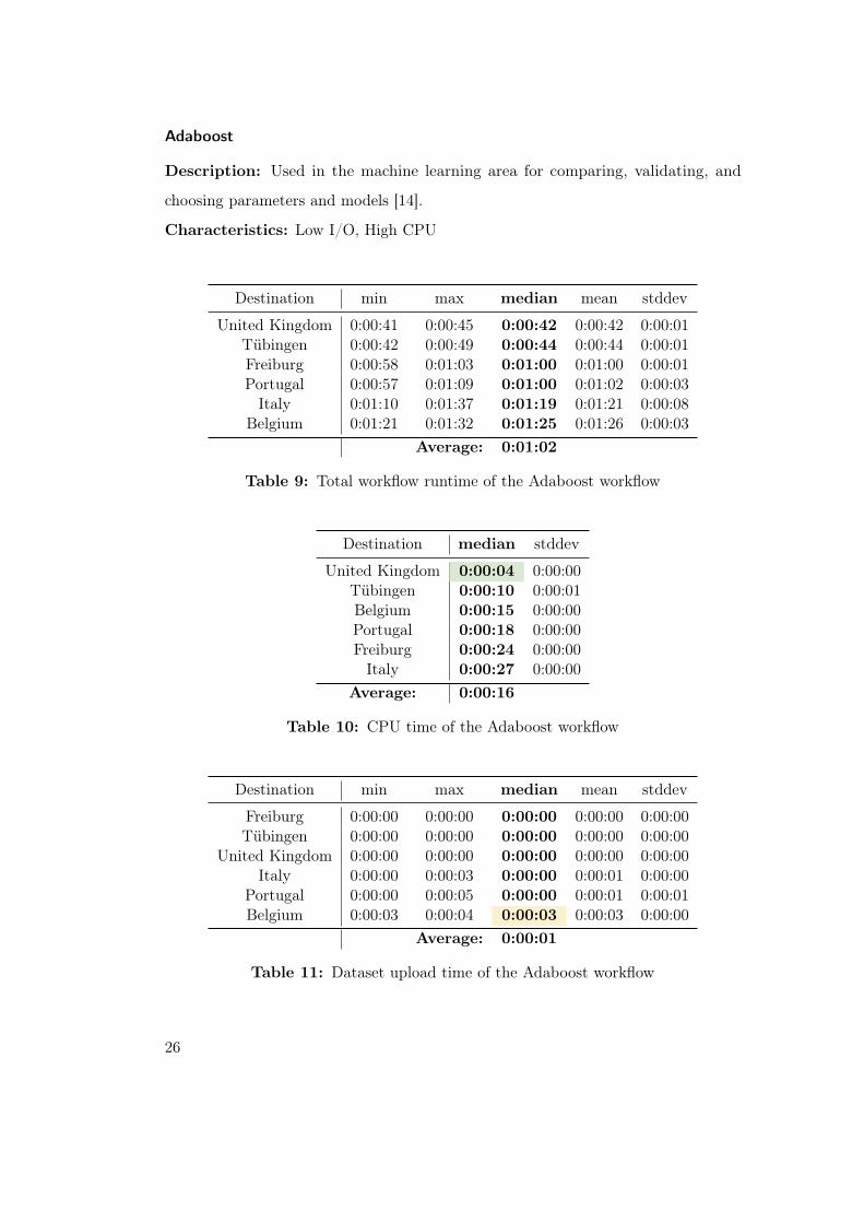
Adaboost

Description: Used in the machine learning area for comparing, validating, and

choosing parameters and models [14].

Characteristics: Low I/O, High CPU


United Kingdom 0:00:41 0:00:45 0:00:42 0:00:42 0:00:01Tübingen 0:00:42 0:00:49 0:00:44 0:00:44 0:00:01Freiburg 0:00:58 0:01:03 0:01:00 0:01:00 0:00:01Portugal 0:00:57 0:01:09 0:01:00 0:01:02 0:00:03Italy 0:01:10 0:01:37 0:01:19 0:01:21 0:00:08

Belgium 0:01:21 0:01:32 0:01:25 0:01:26 0:00:03Average: 0:01:02

Table 9: Total workflow runtime of the Adaboost workflow



Average: 0:00:16

Table 10: CPU time of the Adaboost workflow




Portugal 0:00:00 0:00:05 0:00:00 0:00:01 0:00:01Belgium 0:00:03 0:00:04 0:00:03 0:00:03 0:00:00

Average: 0:00:01

Table 11: Dataset upload time of the Adaboost workflow

26


Freiburg 0:00:00 0:00:00 0:00:00 0:00:00 0:00:00Portugal 0:00:00 0:00:00 0:00:00 0:00:00 0:00:00


Tübingen 0:00:00 0:00:00 0:00:00 0:00:00 0:00:00Belgium 0:00:01 0:00:02 0:00:01 0:00:01 0:00:00

Average: 0:00:00

Table 12: Tool installation time of the Adaboost workflow



United Kingdom 0:00:00 0:00:00 0:00:00 0:00:00 0:00:00Belgium 0:00:00 0:00:00 0:00:00 0:00:00 0:00:00Italy 0:00:00 0:00:00 0:00:00 0:00:00 0:00:00

Portugal 0:00:00 0:00:05 0:00:01 0:00:01 0:00:01Average: 0:00:00

Table 13: Sending results back time of the Adaboost workflow

Destination median


United Kingdom 0:00:00Italy 0:00:00

Portugal 0:00:01Belgium 0:00:04Average: 0:00:01

Table 14: Median sum of staging times of the Adaboost workflow

The results of the Adaboost workflow look similar to Ard. United Kingdom is again

best in total workflow runtime with 42 seconds, Tübingen second with two seconds

more, while Freiburg and Portugal are both in third place with a 1-minute workflow

runtime (Table 9). One interesting result is the standard deviation for the workflow

27

runtime of Italy with eight seconds - five seconds more than Portugal and Belgium,

the next two destinations. This result is also similar to the last workflow and may hint

a trend for the following benchmarks. Again, the staging time of Belgium suggests a

problem in their storage system (Tables 11, 12 and 14).

5.1.2 Benchmarking Bigger, Long Running Workflows

In this category, I benchmarked the destinations with the "Mapping by Sequencing"

and "HiC Explorer" workflows.

Mapping by Sequencing

Description: Used to map lots of fractions of a DNA strand to a reference genome

to combine them into a long DNA strand for further analyzation.

Characteristics: High I/O, High CPU


Tübingen 0:14:27 0:15:50 0:15:04 0:15:05 0:00:22United Kingdom 0:16:48 0:18:18 0:17:03 0:17:07 0:00:21

Freiburg 0:18:33 0:20:35 0:19:03 0:19:16 0:00:29Portugal 0:19:42 0:21:51 0:20:20 0:20:27 0:00:37Belgium 0:23:50 0:24:57 0:24:24 0:24:22 0:00:21Italy 0:28:02 0:31:50 0:30:02 0:29:45 0:01:01

Average: 0:20:59

Table 15: Total workflow runtime of the "Mapping by Sequencing" workflow

28


United Kingdom 0:14:39 0:00:08Tübingen 0:15:43 0:00:06Portugal 0:20:11 0:00:08Freiburg 0:22:18 0:04:39Belgium 0:23:12 0:00:05Italy 0:34:28 0:00:20

Average: 0:23:10

Table 16: CPU time of the "Mapping by Sequencing" workflowAs some tools within the workflow can run in parallel, a longer CPU time compared to the workflow runtime is possible.



Italy 0:01:13 0:03:12 0:01:53 0:01:59 0:00:38Belgium 0:01:55 0:02:16 0:02:08 0:02:06 0:00:06Portugal 0:01:51 0:02:59 0:02:10 0:02:15 0:00:21

United Kingdom 0:03:36 0:03:55 0:03:51 0:03:50 0:00:05

Average: 0:01:49

Table 17: Dataset upload time of the "Mapping by Sequencing" workflow


Freiburg 0:00:00 0:00:00 0:00:00 0:00:00 0:00:00Portugal 0:00:00 0:00:00 0:00:00 0:00:00 0:00:00Tübingen 0:00:00 0:00:00 0:00:00 0:00:00 0:00:00


Belgium 0:00:06 0:00:11 0:00:07 0:00:08 0:00:01

Average: 0:00:01

Table 18: Tool installation time of the "Mapping by Sequencing" workflow

29


Freiburg 0:00:21 0:00:23 0:00:22 0:00:22 0:00:00Tübingen 0:00:18 0:00:32 0:00:22 0:00:23 0:00:04Belgium 0:00:25 0:00:42 0:00:26 0:00:28 0:00:04Portugal 0:00:26 0:01:48 0:00:33 0:00:42 0:00:23Italy 0:00:28 0:01:25 0:00:43 0:00:49 0:00:19

United Kingdom 0:01:59 0:02:27 0:02:11 0:02:10 0:00:07

Average: 0:00:29

Table 19: Sending results back time of the "Mapping by Sequencing" workflow

Destination median


Italy 0:02:36Belgium 0:02:41Portugal 0:02:43

United Kingdom 0:06:02

Average: 0:01:55

Table 20: Median sum of staging times of the "Mapping by Sequencing" workflow

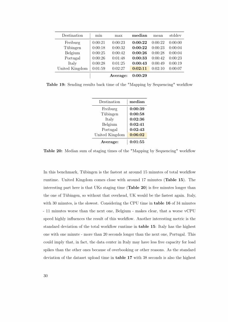
In this benchmark, Tübingen is the fastest at around 15 minutes of total workflow

runtime. United Kingdom comes close with around 17 minutes (Table 15). The

interesting part here is that UKs staging time (Table 20) is five minutes longer than

the one of Tübingen, so without that overhead, UK would be the fastest again. Italy,

with 30 minutes, is the slowest. Considering the CPU time in table 16 of 34 minutes

- 11 minutes worse than the next one, Belgium - makes clear, that a worse vCPU

speed highly influences the result of this workflow. Another interesting metric is the

standard deviation of the total workflow runtime in table 15: Italy has the highest

one with one minute - more than 20 seconds longer than the next one, Portugal. This

could imply that, in fact, the data center in Italy may have less free capacity for load

spikes than the other ones because of overbooking or other reasons. As the standard

deviation of the dataset upload time in table 17 with 38 seconds is also the highest

30

one, it could mean that there are some limitations both in bandwidth, but also on

CPU and storage.

The rest of the dataset upload times in table 17 are as expected: Transferring

750MB is the fastest for Freiburg and Tübingen, as the Galaxy instance from which

the workflows are scheduled is located in the same data center in Freiburg and

connected to the same state-wide academic network (BelWü) as Tübingen. When

the workflow runtime and datset upload time of Portugal and Freiburg are compared,

it is reasonable to conclude that Portugal would probably be faster than Freiburg

if it weren’t for the worse dataset upload time. This information can be a hint for

future routing: Smaller, but long-running jobs may be better send to Portugal than

Freiburg. United Kingdom has the longest total staging time (Table 20) with over

six minutes, so the connection between UK and Freiburg seems to be the slowest.

The fact that United Kingdom, despite the worst staging time, still is in the second

place emphasizes its actual performance lead. Overall, the staging time is dominated

by the dataset upload time.

The tool installation time of Belgium in table 18 with seven seconds, compared to

zero seconds in every other destination, again hints a storage system problem.

HiC Explorer

Description: Used to explore the 3D structure of a DNA strand and how this

structure influences RNA expressions. Applied, among others, in tumor analysis.

Characteristics: High I/O, High Memory, High CPU

Unfortunately, Portugal could not run the workflow properly, as it had problems with

CVMFS (used for some datasets). Because of some work in Tübingen, the staging

time could not be measured at this location. The rest of the locations worked fine.

In this benchmark, 1 + 8 runs were performed.

31



UnitedKingdom 2:12:56 2:40:26 2:21:54 2:23:05 0:07:57Belgium 2:59:05 12:42:09 3:02:39 4:16:36 3:24:24Italy 4:04:58 5:25:16 4:23:01 4:29:09 0:24:53

Average: 2:44:56

Table 21: Total workflow runtime of the "HiC Explorer" workflow


UnitedKingdom 1:49:41 0:03:20Tübingen 2:52:27 0:04:27Freiburg 3:01:51 0:08:08Belgium 4:07:46 0:01:32Italy 6:12:08 0:10:31

Average: 3:36:47

Table 22: CPU time of the "HiC Explorer" workflow


Freiburg 0:03:42 0:04:27 0:03:59 0:04:00 0:00:15Italy 0:22:51 1:21:01 0:38:08 0:40:44 0:18:28

Belgium 0:36:03 0:49:09 0:39:01 0:39:54 0:03:59UnitedKingdom 0:49:43 0:58:13 0:52:33 0:53:44 0:03:17

Tübingen - - - - -

Average: 0:33:25

Table 23: Dataset upload time of the "HiC Explorer" workflow


UnitedKingdom 0:00:37 0:01:36 0:00:48 0:00:54 0:00:19Freiburg 0:01:19 0:01:58 0:01:29 0:01:35 0:00:14Belgium 0:01:23 9:27:53 0:01:53 1:12:39 3:20:06Italy 0:01:42 0:03:47 0:02:03 0:02:15 0:00:40

Tübingen - - - - -

Average: 0:01:15

Table 24: Tool installation time of the "HiC Explorer" workflow

32


Freiburg 0:11:14 0:12:28 0:11:58 0:11:53 0:00:22Belgium 0:14:03 0:40:28 0:15:31 0:18:32 0:08:56Italy 0:27:15 0:58:34 0:41:17 0:41:46 0:11:23

UnitedKingdom 1:00:36 1:53:00 1:04:18 1:10:18 0:17:40Tübingen - - - - -

Average: 0:33:16

Table 25: Sending results back time of the "HiC Explorer" workflow

Destination median

Freiburg 0:17:26Belgium 0:56:25Italy 1:21:28

UnitedKingdom 1:57:39Tübingen -

Average: 1:08:15

Table 26: Median sum of staging times of the "HiC Explorer" workflow

Figure 7: Results of the benchmarkingTotal workflow runtime (left) and total staging time (right) of the "HiCExplorer" workflow per destination.

The results of this benchmark clearly show the impact that the staging time can

have in the case of big datasets. Freiburg with 1:54:32 of total workflow runtime in

table 21 is the fastest, while Tübingen comes close with an eight minutes difference.

United Kingdom is the third fastest, but already takes 2:21:54. However, looking

at the CPU times in table 22 presents a completely opposite picture: This time,

33

United Kingdom is by far the fastest with only 1:49:41, while Freiburg took over

one hour more to process! The total staging time in table 26 explains the reason,

as United Kingdom needed almost two hours for staging, versus Freiburg with only

17:26. If UK had a similar bandwidth like Freiburg, it probably would have a total

workflow runtime of less than an hour. This makes clear that the staging time can

make a huge difference in the overall performance of a workflow!

The rest of the CPU times are as expected: Italy took the longest to process

with 6:12:08, two hours more than Belgium with 4:07:46, which again confirms the

assumption that Italy has the slowest vCPUs. Interestingly, United Kingdom took

the least amount of time for checking the needed tools (Table 24) with only 48

seconds. This result may hint a good performing storage system, which would also

partly explain the good CPU time of United Kingdom, as I/O-wait is included in

this measure.

5.1.3 Benchmarking Workflows with many Files

Docking with Vina

Description: Used to simulate and explore the interaction between a molecule (for

example a possible drug candidate) with a protein.

Characteristics: Low I/O, Lot of files, High CPU


United Kingdom 0:02:00 0:02:18 0:02:10 0:02:09 0:00:05Freiburg 0:03:02 0:03:18 0:03:11 0:03:10 0:00:04Tübingen 0:03:04 0:03:20 0:03:12 0:03:12 0:00:05

Italy 0:03:47 0:06:09 0:04:26 0:04:27 0:00:35Portugal 0:06:09 0:06:40 0:06:22 0:06:21 0:00:07Belgium 0:07:55 0:17:13 0:09:01 0:09:36 0:02:16

Average: 0:04:44

Table 27: Total workflow runtime of the "Docking with Vina" workflow

34



Average: 0:41:03

Table 28: CPU time of the "Docking with Vina" workflow



United Kingdom 0:00:24 0:00:29 0:00:26 0:00:26 0:00:01Portugal 0:00:43 0:01:30 0:00:44 0:00:47 0:00:11Italy 0:00:29 0:02:41 0:01:05 0:01:15 0:00:37

Belgium 0:02:35 0:03:58 0:02:56 0:02:59 0:00:23Average: 0:00:55

Table 29: Dataset upload time of the "Docking with Vina" workflow


Freiburg 0:00:02 0:00:02 0:00:02 0:00:02 0:00:00Portugal 0:00:02 0:00:24 0:00:02 0:00:03 0:00:05

United Kingdom 0:00:03 0:00:03 0:00:03 0:00:03 0:00:00Tübingen 0:00:04 0:00:13 0:00:07 0:00:07 0:00:03

Italy 0:00:03 0:01:21 0:00:29 0:00:30 0:00:22Belgium 0:02:06 0:03:24 0:02:33 0:02:35 0:00:22

Average: 0:00:33

Table 30: Tool installation time of the "Docking with Vina" workflow

35




Portugal 0:00:23 0:00:29 0:00:24 0:00:24 0:00:01Belgium 0:00:21 0:00:56 0:00:30 0:00:32 0:00:09

Average: 0:00:19

Table 31: Sending results back time of the "Docking with Vina" workflow

Destination median


United Kingdom 0:00:49Portugal 0:01:10Italy 0:01:55

Belgium 0:05:59Average: 0:01:47

Table 32: Median sum of staging times of the "Docking with Vina" workflow

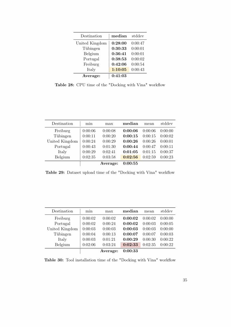
United Kingdom is the fastest in total workflow runtime, see table 27, with only

02:10, Freiburg and Tübingen are slightly slower with 03:11 and 03:12. The number of

available cores for the whole cluster is one of the dominating factors in this workflow,

as it can be seen by the comparison of the performance of Italy (80 cores) with 04:26

versus Portugal (8 cores) with 06:22.

This workflow offers an almost perfect view into the performance of the vCPUs at

each location, as the I/O needs of the used tools and therefore the I/O-wait times

are very low: Belgium, being in the third place of the CPU times in table 28, shows

that their vCPUs are comparably fast to the other destinations - again a hint for a

bad-performing file system. Freiburg, on the other hand, seems to have one of the

less performant CPUs compared to the others. The CPU time of Italy, with 01:10:05,

again shows that their vCPUs are the slowest performance-wise.

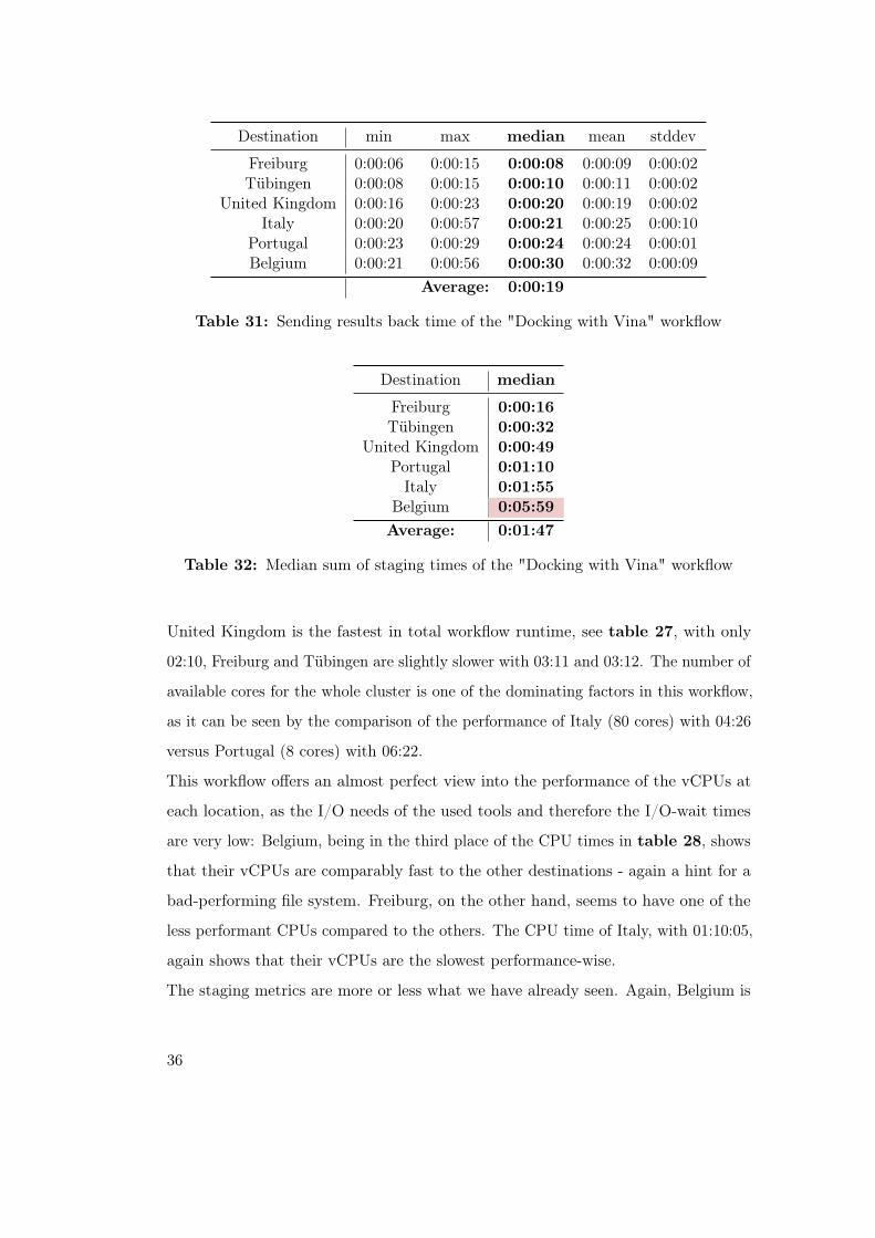
The staging metrics are more or less what we have already seen. Again, Belgium is

36

in the last place with almost three minutes for just receiving the datasets (Table 29)

and two and a half minutes for checking tools that are already installed (Table 30) -

again, a clear sign of a bad file system performance. The tool installation time of

Tübingen is the other interesting result with seven seconds - five more than Freiburg

and Portugal. As this metric is I/O-bound, it could be a sign, that the file system

performance of Freiburg and Portugal is a bit better than the one of Tübingen and

that Freiburg and Portugal have similar performance characteristics.

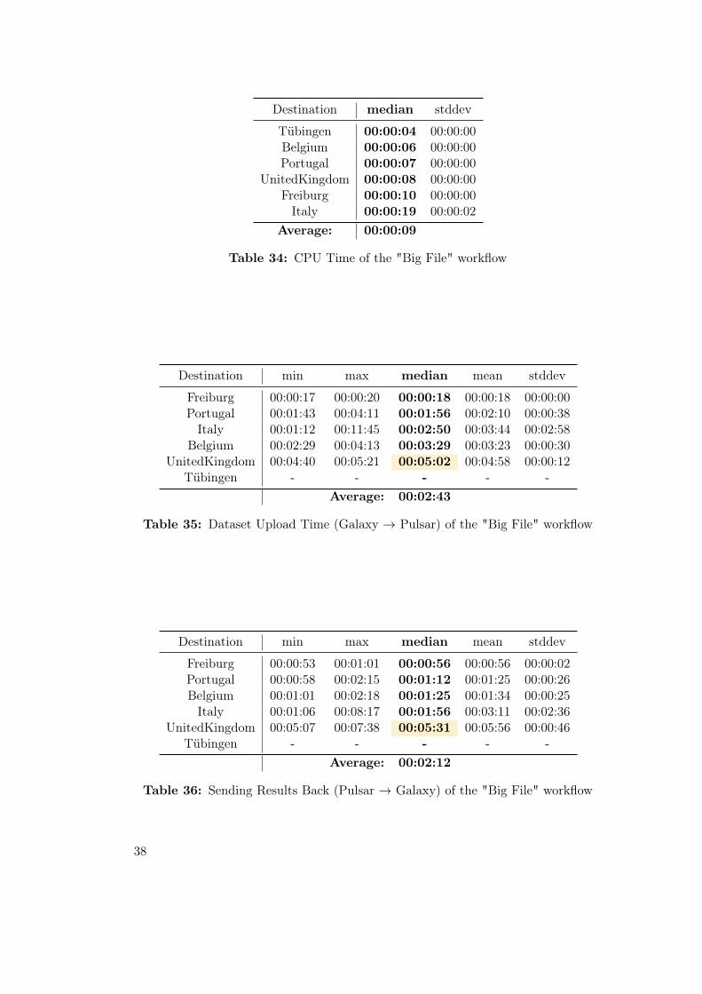
5.1.4 Benchmarking the Connection Speed of Destinations

To test the connection speeds between the Galaxy instance in Freiburg and the other

destinations, I build a very simple workflow, that sends a 1GB file to the destinations

and returns it back to Galaxy. In this way, we can approximate the transfer speeds.

While doing this benchmark, Tübingen had a problem with returning the staging

times. Therefore, the speed of Tübingen is an approximation using the workflow

runtime and the results of the other destinations. As Galaxy further processes datasets

to determine the metadata like file type (which takes some additional time and is

included in this metric), the speed of Pulsar → Galaxy won’t reflect the full potential

of the connection.


Freiburg 00:01:57 00:02:27 00:02:19 00:02:18 00:00:06Tübingen 00:03:14 00:04:10 00:03:27 00:03:33 00:00:15Portugal 00:03:22 00:06:26 00:03:46 00:04:19 00:00:59Italy 00:03:23 00:21:25 00:05:16 00:08:00 00:05:36


Average: 00:05:28

Table 33: Total Workflow Runtime of the "Big File" workflow

37


Tübingen 00:00:04 00:00:00Belgium 00:00:06 00:00:00Portugal 00:00:07 00:00:00

UnitedKingdom 00:00:08 00:00:00Freiburg 00:00:10 00:00:00Italy 00:00:19 00:00:02

Average: 00:00:09

Table 34: CPU Time of the "Big File" workflow


Freiburg 00:00:17 00:00:20 00:00:18 00:00:18 00:00:00Portugal 00:01:43 00:04:11 00:01:56 00:02:10 00:00:38Italy 00:01:12 00:11:45 00:02:50 00:03:44 00:02:58


Tübingen - - - - -Average: 00:02:43

Table 35: Dataset Upload Time (Galaxy → Pulsar) of the "Big File" workflow


Freiburg 00:00:53 00:01:01 00:00:56 00:00:56 00:00:02Portugal 00:00:58 00:02:15 00:01:12 00:01:25 00:00:26Belgium 00:01:01 00:02:18 00:01:25 00:01:34 00:00:25Italy 00:01:06 00:08:17 00:01:56 00:03:11 00:02:36

UnitedKingdom 00:05:07 00:07:38 00:05:31 00:05:56 00:00:46Tübingen - - - - -

Average: 00:02:12

Table 36: Sending Results Back (Pulsar → Galaxy) of the "Big File" workflow

38

Destination Galaxy → Pulsar Pulsar → Galaxy

Freiburg 55.56 MB/s 17.86 MB/sTübingen ≈ 10 MB/s ?Portugal 8.62 MB/s 13.89 MB/sItaly 5.88 MB/s 8.62 MB/s

Belgium 4.78 MB/s 11.76 MB/sUnited Kingdom 3.31 MB/s 3.02 MB/s

Table 37: Approximate transfer speeds based on staging times of the "Big File"workflow

The results in table 37 look similar to the previous results of the other benchmarks.

The transfer to Freiburg is because of the locality the fastest. Transferring one big

file seems to perform similarly in Tübingen and Portugal, even though Tübingen is

better connected. United Kingdom clearly has the slowest connection speed, but as

the other tests have shown, most of the time its overall performance advantage can

compensate for that.

5.1.5 Conclusions of the Destination Comparison

Figure 8: Results of the benchmarkingTotal workflow runtime (left) and total staging time (right) by workflowand destination.

A chart of the "HiC Explorer" workflow can be found in figure 7.

Considering the overall workflow runtime of all the benchmarks that were done,

United Kingdom is the fastest overall. Especially the CPU times were always the

lowest, which indicates a very good CPU performance, but also a good storage

39

system performance, as I/O-wait time is included in this measure too. Even though

United Kingdom has the slowest connection speed of all tested destinations, its overall

performance advantage could mostly compensate for that. However, for workflows

that have very big datasets like "HiC Explorer", a location with better transfer

speeds should be considered. Tübingen, the second-fastest destination according to

the tests, comes close to the performance of United Kingdom. The vCPUs and the

storage system are similarly performant, but it has one advantage: Since Freiburg

(the hosting location of UseGalaxy.eu) and Tübingen are well connected, the dataset

transfer part of the staging time is one of the best. So Tübingen might be a good

fit for workflows that are big in file size, compute- and I/O-intensive. If the size of

the dataset is smaller, Portugal should be considered: The vCPUs seem to be in a

similar performance-range as Tübingen, but the connection and therefore the staging

time is less optimal.

Italy, in fifth place, has a moderate performance, which can vary a bit sometimes.

The CPU time has in all benchmarks been the longest (by up to two hours longer in

the case of "HiC Explorer") even in cases where the I/O-needs were low, so we can

conclude that their vCPUs are the slowest, or that they at least offer the lowest mean

speed for a vCPU because of overbooking or other factors. The destination could

be useful for workflows with a lot of small requests, as, in total, the cluster in Italy

currently has the second most number of vCPUs currently available. In these cases,

a workflow (like "Docking with Vina") can still be processed faster, even though the

vCPUs are slower.

Belgium is the slowest. The results from Belgium suggest that this performance has

something to do with the storage system, as tool installation times (which is highly

I/O bound) were mostly a few seconds behind every other destination. Another

indicator were the benchmarks with the Ard and Adaboost workflows: Both have low

I/O needs and in these cases, the CPU time of Belgium was in the second place both

times. So probably the available vCPUs are not bad at all, but the I/O-performance

drags everything else down. However, for workloads where I/O is less of a priority

40

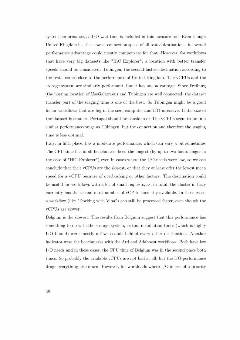
and datasets are moderately sized, Belgium can still be a good fit.

Destination Pros ↑ Cons ↓ Best for

United Kingdom CPU, StorageSystem

Connection Medium Datasets,High I/O, High CPU

Tübingen CPU, StorageSystem, Connection(well connected toFreiburg)

Big Datasets, HighI/O, High CPU

Freiburg Storage System,Connection (samedata center)

Big Datasets, HighI/O, High CPU

Portugal CPU, StorageSystem

Connection Small/MediumDatasets, High I/O,High CPU

Italy Storage System,vCPU count

CPU High I/O,Low/Medium CPU,

Belgium CPU Storage System(I/O-Performance),Connection

Small Datasets, LowI/O, High CPU

Table 38: Summary of the Destination Comparison

41

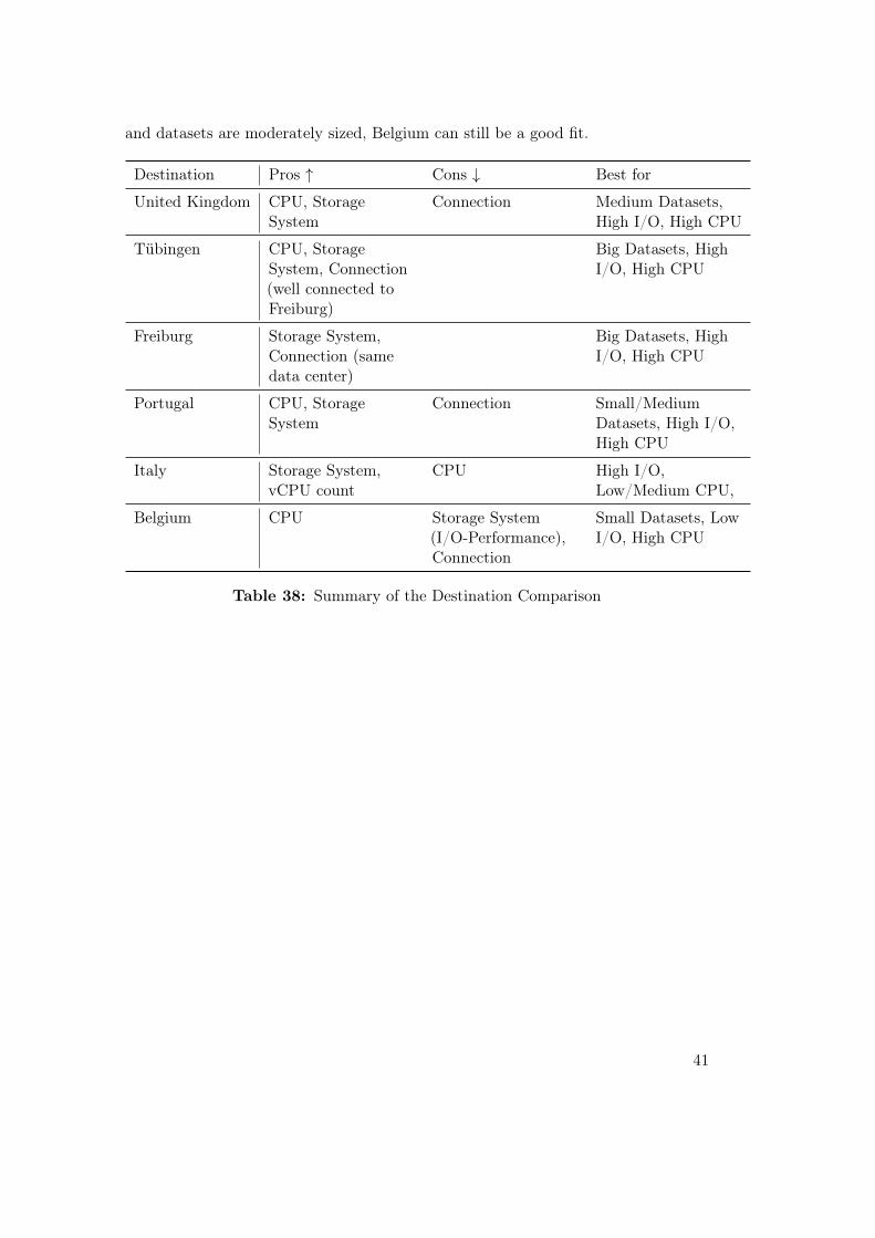
5.2 Determining Staging Time on a Freshly Installed

Pulsar Instance

To figure out, what the overhead for a Pulsar instance that is started for the first

time is, I created a "Cold vs Warm" benchmark. While preparing, I thought of some

possible scenarios of a cold start benchmark:

a) Remove all virtual environments and dependencies ("tools"-folder on Pulsar)

b) Clear the cache of CVMFS and remove all files persisted to Pulsar

c) Do a) and b) combined

a) measures the additional time needed to install tools for the first time, while

b) focuses on the situations where everything is installed, but new datasets are

processed and therefore need to be downloaded for the first time. Unfortunately,

because of the long runtime of this kind of benchmark together with the focus on the

destination comparisons, I did not have the time to benchmark b) and c), so I only

benchmarked the tool installation times. Additionally, due to problems with Conda,

not all workflows from the previous benchmark could be used. In the end, I focused

on Ard, Adaboost, and Mapping by Sequencing.

The following setup was used:

Type Quantity Flavour vCPU RAM

Galaxy Server 1 m1.xxlarge 16 32GBPulsar Sever 1 m1.xlarge 8 16GBNFS 1 m1.large 4 8GBCentral Manager 1 m1.medium 2 4GBExecute Node 2 m1.large 4 8GB

Table 39: Instances used in Cold vs Warm Benchmark

42

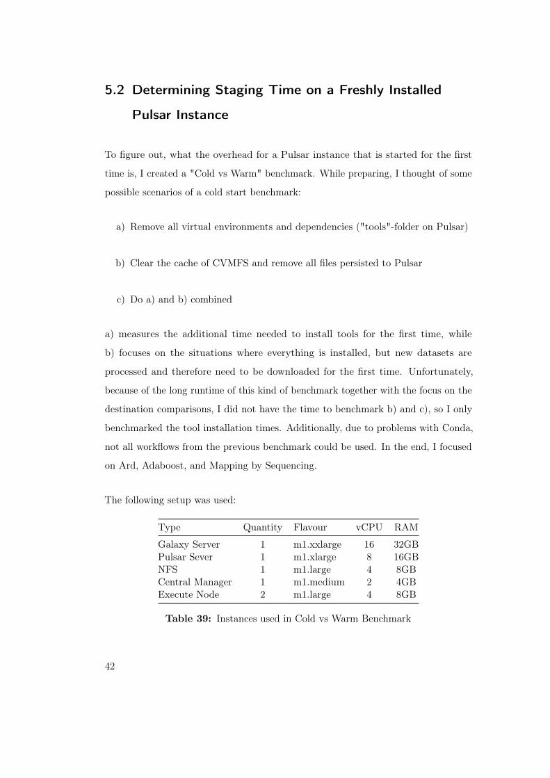
For every workflow, a cold benchmark was performed 15 times by replacing the

"_conda" folder (which contains all the dependencies) with a fresh one, where no

dependencies except the basic ones are installed. After that, the workflow ran for 1 +

15 times in the "warm" state, while the results of the first run were not considered.

5.2.1 ResultsWorkflow Cold Warm Difference Factor

Adaboost 0:08:10 0:00:47 0:07:23 10.43Ard 0:08:20 0:00:45 0:07:35 11.11Mapping by Sequencing 0:27:53 0:17:52 0:10:01 1.56

Table 40: Median total workflow runtimes of the Cold vs Warm benchmark

Workflow Cold Warm Difference

Adaboost 00:00:16 00:00:14 00:00:02Ard 00:00:15 00:00:14 00:00:01

Mapping by Sequencing 00:20:21 00:20:10 00:00:11

Table 41: Median CPU time of the Cold vs Warm benchmark

Workflow Cold Runtime Difference - Tool Installation Time

Adaboost 00:07:18 0:00:05Ard 00:07:29 0:00:06

Mapping by Sequencing 00:09:50 0:00:11

Table 42: Median Tool Installation Time of the Cold vs Warm benchmark"Runtime Difference - Tool Installation Time" means the overhead left, after the mediantool installation time is subtracted from the median total runtime differences between a coldand a warm run.

The differences of the median total workflow runtimes in table 40 are between seven

to ten minutes. As Ard and Adaboost consist of only two tools, seven minutes can

probably be seen as a rough lower bound of the dependency resolution. For more or

bigger dependencies, ten minutes could presumably easily be surpassed. Looking at

the differences of the CPU times in table 41, only Mapping by Sequencing seem to

43

have a noticeable overhead, but as I just tested three workflows, we can not clearly

confirm, that this overhead really stems from the cold run. However, looking at the

values from table 42 at least hint an additional overhead somewhere.

44

5.3 Stress Testing HTCondor Clusters

Besides benchmarking Pulsar, a stress test of HTCondor was performed. The aim was

to see how it handles huge amounts of small jobs and what happens if some instances,

like an execution node or even the central manager, fail while processing: Will all

jobs still complete? The purpose of this type of test was to figure out if Galaxy needs

to handle those cases or if it could solely rely on HTCondor to restart failed jobs.

The following scenarios were tested, while n amount of jobs were scheduled:

• Repeatedly reboot the central manager at 5-minute intervals

• Kill and replace the central manager during the test

• Repeatedly reboot a random execution node

• Repeatedly kill and replace a random execution node

#!/bin/bash

sleep 1

echo "$(hostname)"

Figure 9: Simple test-job

The actual jobs were quite simple, consisting of sleeping

for one second and writing the hostname of the execution

node to the output.

The setup consisted of the following instances:

Type Quantity Flavour # vCPUs RAM

Central Manager 1 m1.medium 2 4GBSubmit Node 1 m1.medium 2 4GBNFS 1 m1.medium 2 4GBExecute Node 4 m1.small 1 2GB

Table 43: Instances used in HTCondor stresstest

The "Burst" benchmark type (see Chapter 4.3.3) was used in this test, allowing to

submit multiple jobs at the same time via my benchmarking framework. For the

submission and monitoring part, I extended the GalaxyBenchmarker to use a "Condor-

Destination". It sends the job file to the submit-node using an Ansible-Playbook and

45

uses SSH for the "condor_submit"-command. The "condor_q"-command is called

every second for monitoring the jobs. After the jobs are finished, the JSON-Output

of "condor_history" is used for getting all the metrics, like runtime (wall-clock time),

back.

For rebooting and rebuilding instances, I built some background-tasks that could be

triggered every x-seconds for a set amount of time. They use the OpenStack-SDK for

sending reboot- and even rebuild-commands for a given instance-class (specified by

name) to the OpenStack manager.

5.3.1 Determining the Submit RateOne of the first steps was to figure out how many jobs HTCondor can handle

in a reasonable amount of time. In this case, the actual submission turned out

to be a bottleneck: Submitting 1 million jobs was not feasible, as it, on the

one hand, already exceeded the default-setting of HTCondor for the maximum

amount of jobs per submission and user (MAX_JOBS_PER_SUBMISSION and

MAX_JOBS_PER_OWNER), and, on the other hand, failed after submitting for

around an hour. Also, the submission of 100k jobs failed similarly ("Failed to commit

job submission into the queue"). Submitting these huge amounts of jobs makes

Jobs Submit-Threads Duration Submits per second

1 Mio 1 Fail after 1h –100k 1 Fail after 1h –50k 1 31m (1919s) 26.0520k 1 11.85m (711s) 28.1310k 1 6.25m (374s) 26.710k (2 x 5k) 2 4.08m (245s) 40.85k 1 3.15m (189s) 26.465k (2 x 2.5k) 2 2m (119s) 421k 1 38s 26.3

Table 44: Submit-DurationsThe tests were done with one or two threads simultaneously, measuringhow long HTCondor needs to successfully process the submission.

HTCondor unresponsive for additional requests, even though the CPU-Utilization of

46

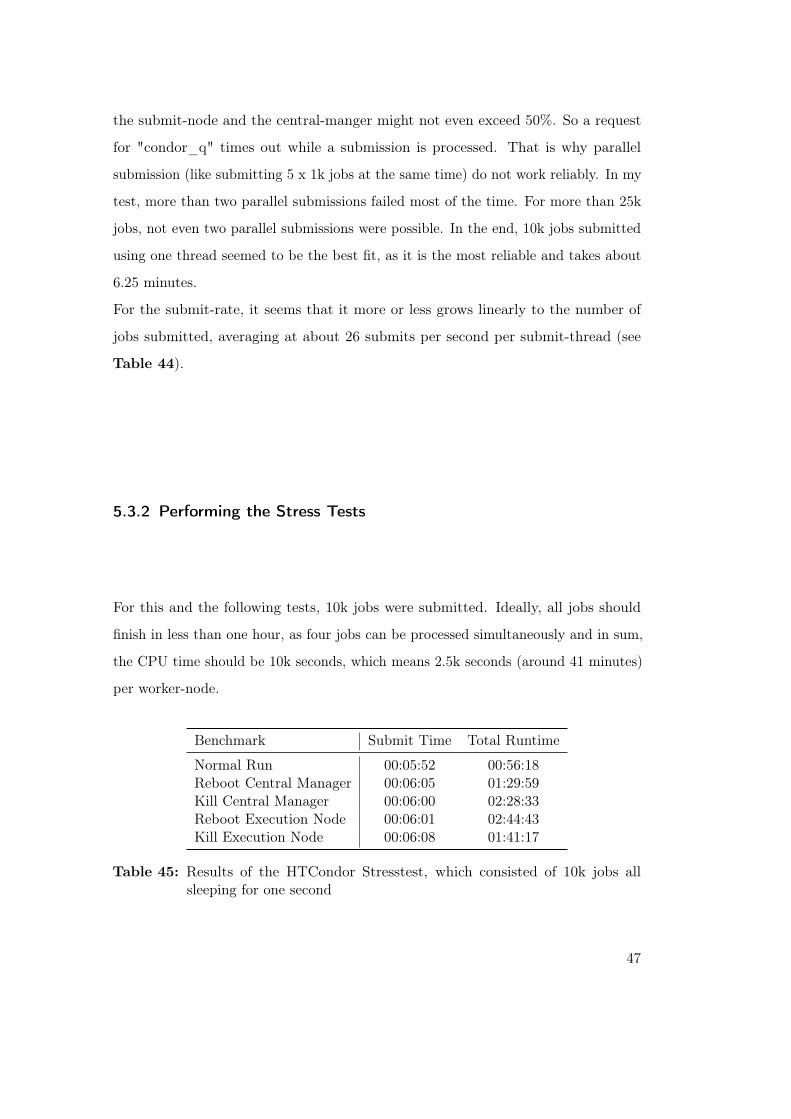
the submit-node and the central-manger might not even exceed 50%. So a request

for "condor_q" times out while a submission is processed. That is why parallel

submission (like submitting 5 x 1k jobs at the same time) do not work reliably. In my

test, more than two parallel submissions failed most of the time. For more than 25k

jobs, not even two parallel submissions were possible. In the end, 10k jobs submitted

using one thread seemed to be the best fit, as it is the most reliable and takes about

6.25 minutes.

For the submit-rate, it seems that it more or less grows linearly to the number of

jobs submitted, averaging at about 26 submits per second per submit-thread (see

Table 44).

5.3.2 Performing the Stress Tests

For this and the following tests, 10k jobs were submitted. Ideally, all jobs should

finish in less than one hour, as four jobs can be processed simultaneously and in sum,

the CPU time should be 10k seconds, which means 2.5k seconds (around 41 minutes)

per worker-node.

Benchmark Submit Time Total Runtime

Normal Run 00:05:52 00:56:18Reboot Central Manager 00:06:05 01:29:59Kill Central Manager 00:06:00 02:28:33Reboot Execution Node 00:06:01 02:44:43Kill Execution Node 00:06:08 01:41:17

Table 45: Results of the HTCondor Stresstest, which consisted of 10k jobs allsleeping for one second

47

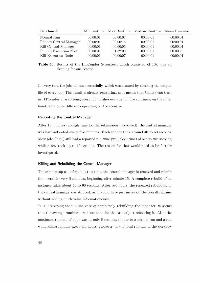
Benchmark Min runtime Max Runtime Median Runtime Mean Runtime

Normal Run 00:00:01 00:00:07 00:00:01 00:00:01Reboot Central Manager 00:00:01 00:00:16 00:00:01 00:00:01Kill Central Manager 00:00:01 00:00:06 00:00:01 00:00:01Reboot Execution Node 00:00:01 01:32:09 00:00:01 00:00:25Kill Execution Node 00:00:01 00:00:07 00:00:01 00:00:01

Table 46: Results of the HTCondor Stresstest, which consisted of 10k jobs allsleeping for one second

In every test, the jobs all ran successfully, which was ensured by checking the output-

file of every job. This result is already reassuring, as it means that Galaxy can trust

in HTCondor guaranteeing every job finishes eventually. The runtimes, on the other

hand, were quite different depending on the scenario.

Rebooting the Central Manager

After 15 minutes (enough time for the submission to succeed), the central manager

was hard-rebooted every five minutes. Each reboot took around 40 to 50 seconds.

Most jobs (9961) still had a reported run time (wall-clock time) of one to two seconds,

while a few took up to 16 seconds. The reason for that would need to be further

investigated.

Killing and Rebuilding the Central-Manager

The same setup as before, but this time, the central manager is removed and rebuilt

from scratch every 5 minutes, beginning after minute 15. A complete rebuild of an

instance takes about 50 to 60 seconds. After two hours, the repeated rebuilding of

the central manager was stopped, as it would have just increased the overall runtime

without adding much value information-wise.

It is interesting that in the case of completely rebuilding the manager, it seems

that the average runtimes are lower than for the case of just rebooting it. Also, the

maximum runtime of a job was at only 6 seconds, similar to a normal run and a run

while killing random execution nodes. However, as the total runtime of the workflow

48

is, with 02:28:33, almost one hour longer than just rebooting the central manager,

the reason for the shorter runtimes could be because of losing track of some jobs and

their runtime, while still being able to complete the job.

Rebooting Execution Nodes

After minute 15, a random execution node was hard-rebooted every 30 seconds. After

a reboot, the node began accepting new jobs as usual, while jobs that failed due

to the reboot stayed in the run-state for around 40 to 45 minutes. Therefore most

of the jobs completed within one second, but some (81 jobs) report a runtime of

around 46 minutes. One poor job even had a runtime of 01:32:09: It probably was

scheduled two times on nodes that were rebooted at that moment. This behavior

indicates that HTCondor allows jobs to run for a set amount of time without needing

to communicate back. If this time is exceeded, the job will be resubmitted. My

observations confirm the behavior of the so-called "Job Leases". The manual [15]

describes them as the following:

A job lease specifies how long a given job will attempt to run on a remote

resource, even if that resource loses contact with the submitting machine.

Similarly, it is the length of time the submitting machine will spend

trying to reconnect to the (now disconnected) execution host, before the

submitting machine gives up and tries to claim another resource to run

the job.

The default configuration-value of JobLeaseDuration is set at 40 minutes, which also

comes close to the observed 40 to 46 minutes of jobs stuck after a reboot.

Killing and Rebuilding Execution Nodes

In the last test, after minute 15, an arbitrary execution node was killed and rebuilt

every 30 seconds. The results are a bit confusing, as they differ to the last test of

just rebooting the nodes: The total runtime is more than one hour less with 01:44:17

and the maximum runtime per job at only seven seconds. Apparently, a complete

49

kill is better for the runtime than just rebooting an execution-node. The reason for

that is unclear and would need to be further investigated.

50

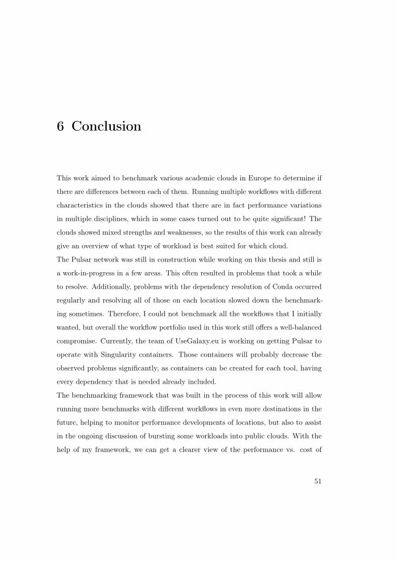
6 Conclusion

This work aimed to benchmark various academic clouds in Europe to determine if

there are differences between each of them. Running multiple workflows with different

characteristics in the clouds showed that there are in fact performance variations

in multiple disciplines, which in some cases turned out to be quite significant! The

clouds showed mixed strengths and weaknesses, so the results of this work can already

give an overview of what type of workload is best suited for which cloud.

The Pulsar network was still in construction while working on this thesis and still is

a work-in-progress in a few areas. This often resulted in problems that took a while

to resolve. Additionally, problems with the dependency resolution of Conda occurred

regularly and resolving all of those on each location slowed down the benchmark-

ing sometimes. Therefore, I could not benchmark all the workflows that I initially

wanted, but overall the workflow portfolio used in this work still offers a well-balanced

compromise. Currently, the team of UseGalaxy.eu is working on getting Pulsar to

operate with Singularity containers. Those containers will probably decrease the

observed problems significantly, as containers can be created for each tool, having

every dependency that is needed already included.

The benchmarking framework that was built in the process of this work will allow

running more benchmarks with different workflows in even more destinations in the

future, helping to monitor performance developments of locations, but also to assist

in the ongoing discussion of bursting some workloads into public clouds. With the

help of my framework, we can get a clearer view of the performance vs. cost of

51

different cloud providers and instance types and determining if there are advantages

in utilizing a public cloud. Additionally, there are already ideas to benchmark dif-

ferent implementations of Galaxy job-runners for performance improvements and to

benchmark other features of Galaxy to determine if they may have a negative impact

on the overall performance. These are just some of many imaginable use cases of this

framework in the future.

The stress test of HTCondor strengthens the trust in its ability to recover from failures:

In all of the tests, each submitted job successfully ran at some point. However, the

runtimes of each test varied. The reason for that would need to be further studied,

but as the main focus was on benchmarking the Pulsar locations, I did not have

enough time for this task.

52

7 Acknowledgments

I would like to thank everyone who has helped me with this thesis:

• Björn Grüning as my advisor for always being open to questions and explaining

tools and methods that were new to me, but also for suggestions that clearly

helped to get my thesis to this state.

• Gianmauro Cuccuru for always helping with Pulsar and Galaxy, supporting me

in finding the bugs in my configurations or fixing problems when, again(!), a

workflow arbitrarily failed at one Pulsar location.

• Björn Grüning, Anika Erxleben and Dominik Aigner for proofreading this thesis,

finding a bunch of mistakes and unclear sentences, that I would have probably

overread on my own.

• The whole team of Galaxy Freiburg for being very welcoming to this new

bachelor student.

• Also, the sponsor and providers of the infrastructure used in this thesis. Espe-

cially the ELIXIR network. But also the BW Cloud and the Rechenzentrum of

the University of Freiburg for providing resources generously.

53

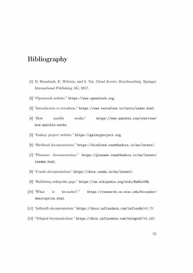
Bibliography

[1] D. Bermbach, E. Wittern, and S. Tai, Cloud Service Benchmarking. Springer

International Publishing AG, 2017.

[2] “Openstack website.” https://www.openstack.org.

[3] “Introduction to terraform.” https://www.terraform.io/intro/index.html.

[4] “How ansible works.” https://www.ansible.com/overview/

how-ansible-works.

[5] “Galaxy project website.” https://galaxyproject.org.

[6] “Bioblend documentation.” https://bioblend.readthedocs.io/en/latest/.

[7] “Planemo documentation.” https://planemo.readthedocs.io/en/latest/

readme.html.

[8] “Conda documentation.” https://docs.conda.io/en/latest/.

[9] “Rabbitmq wikipedia page.” https://en.wikipedia.org/wiki/RabbitMQ.

[10] “What is htcondor?.” https://research.cs.wisc.edu/htcondor/

description.html.

[11] “Influxdb documentation.” https://docs.influxdata.com/influxdb/v1.7/.

[12] “Telegraf documentation.” https://docs.influxdata.com/telegraf/v1.12/.

55

https://www.openstack.org

https://www.terraform.io/intro/index.html

https://www.ansible.com/overview/how-ansible-works

https://www.ansible.com/overview/how-ansible-works

https://galaxyproject.org

https://bioblend.readthedocs.io/en/latest/

https://planemo.readthedocs.io/en/latest/readme.html

https://planemo.readthedocs.io/en/latest/readme.html

https://docs.conda.io/en/latest/

https://en.wikipedia.org/wiki/RabbitMQ

https://research.cs.wisc.edu/htcondor/description.html

https://research.cs.wisc.edu/htcondor/description.html

https://docs.influxdata.com/influxdb/v1.7/

https://docs.influxdata.com/telegraf/v1.12/

[13] “Grafana documentation.” https://grafana.com/docs/v4.3/.

[14] “scikit-learn - homepage.” https://scikit-learn.org/stable/.

[15] “Htcondor manaual - special environment considerations.”

https://htcondor.readthedocs.io/en/v8_9_2/users-manual/

special-environment-considerations.html#job-leases.

56

https://grafana.com/docs/v4.3/

https://scikit-learn.org/stable/

https://htcondor.readthedocs.io/en/v8_9_2/users-manual/special-environment-considerations.html#job-leases

https://htcondor.readthedocs.io/en/v8_9_2/users-manual/special-environment-considerations.html#job-leases

benchmarking big-data workflows across european academic

Documents