benchmarking of several material constitutive models for
TRANSCRIPT

1
Benchmarking of several material constitutive models for
tribology, wear, and other mechanical deformation
simulations of Ti6Al4V
Cen Liua, Saurav Goela*, Iñigo Llavorib, Pietro Stolfc, Claudiu Giuscaa, Alaitz
Zabalab, Joern Kohlscheend, Jose Mario Paivac, Jose L Endrinoa, Stephen C.
Veldhuisc and German S. Fox Rabinovichc
aSchool of Aerospace, Transport and Manufacturing, Cranfield University, MK430AL, UK bSurface Technologies, Mondragon University, Loramendi 4, 20500 Arrasate, Mondragon, Spain
cMcMaster Manufacturing Research Institute, (MMRI), McMaster University, Hamilton, Ontario, Canada dKennametal Shared Services Gmbh, Altweiherstr 27-31, Ebermannstadt 91320, Germany
* Corresponding author. Tel.: +44-1234-754132; E-mail address: [email protected]
Abstract
Use of an alpha-beta (multiphase HCP-BCC) titanium alloy, Ti6Al4V, is ubiquitous in
a wide range of engineering applications. The previous decade of finite element analysis
research on various titanium alloys for numerous biomedical applications especially in
the field of orthopedics has led to the development of more than half a dozen material
constitutive models, with no comparison available between them. Part of this problem
stems from the complexity of developing a vectorised user-defined material subroutine
(VUMAT) and the different conditions (strain rate, temperature and composition of
material) in which these models are experimentally informed. This paper examines the
extant literature to review these models and provides quantitative benchmarking against
the tabulated material model and a power law model of Ti6Al4V taking the test case of
a uniaxial tensile and cutting simulation.
Keywords: Ti6Al4V; Material models; Johnson-Cook model; Zerilli Armstrong
model; Voyiadjis-Abed model; tensile test; cutting

2
1. Introduction
The ubiquitous use of titanium alloys in disparate fields like aerospace, automotive and
the biomedical industry makes research on material characteristics of Ti6Al4V
rewarding. In addition to achieving lighter weight, high corrosion resistance and high
specific strength makes titanium alloys an ideal choice for biomedical manufacturing
(Inagaki, Takechi et al. 2014). However, machining titanium alloys is a daunting task
and they are generally referred to as “difficult to machine” materials. As a continuous
research effort in improving our understanding on the material response of Ti6Al4V
under different loading conditions, finite element analysis (FEA) has become an
established simulation tool for predictive assessment of different kinds of
manufacturing and material characterisation processes.
This kind of research is helpful in identification of the right combination of tooling
material, optimisation of the processing window and development of strategies for
suppressing tool wear which are all major research drivers in manufacturing.
In modern competitive markets, many industries have developed commercial softwares
to perform FEA, each having their own advantages. Beside many others, the most
common FEA software packages that are used to simulate machining processes are
DEFORM, AdvantEdge, Abaqus, ANSYS and LS-DYNA. Usually, these codes have
their own material library database built on an experimentally observed understanding
of the material’s behaviour under a given set of stress-strain conditions. In many
situations, where complex material models are proposed, user subroutines are to be
coded to work in these packages as incorporation of all material models within one
package will make the software extremely bulky and complicated. Moreover, it is a
continuous process, for instance over the past few years, more than half a dozen
material constitutive models have been proposed for Ti6Al4V alone and it is high time
3
that these models be benchmarked and compared to assert their proximity with each
other. Some of the notable material models proposed for Ti6Al4V are the Arrhenius-
type constitutive equation (Mosleh, Mikhaylovskaya et al. 2017), the Field-Backofen
model, the Khan-Huang-Liang model, the Mechanical Threshold Stress model
(Kotkunde, Deole et al. 2014), the Johnson-Cook model (Yadav, Bajpai et al. 2017),
the Multi-Branch model (Yameogo, Haddag et al. 2017), the Tangent hyperbolic model
(Xiulin, Shiguang et al. 2015), the Voyiadjis-Abed model (Tabei, Abed et al. 2017), the
Zerilli-Armstrong model (Che, Zhou et al. 2018), the Baker Modification of EI-Magd
model (Alvarez, Domingo et al. 2011) and the Cuitino and Ortiz model (Man, Ren et
al. 2012).
However, it may be noted that these material models are developed under different
experimental conditions and due to this, it is challenging to say which particular
material model is the best. It is also worth noting that the implementation of all these
complex material models is not that straightforward and developing the user subroutine
like VUMAT consumes significant time for testing each of the models. Consequently,
the motivation of this paper was to compare several of these material models to
establish the variation in the results presented by them for a given problem and then to
benchmark the models against the predictions made by commercial codes like
AdvantEdge and DEFORM. These two are commercially popular codes used by the
machining community and have their own way of describing the material constitutive
model, AdvantEdge, for example, implements the Cuitino and Ortiz model (Man, Ren
et al. 2012) while DEFORM implements a tabulated material model of the form 𝜎 =𝜎(𝜀,̅ 𝜀̇, 𝑇), where 𝜎, 𝜀 ,̅ 𝜀̇ and T refer to flow stress, equivalent plastic strain, equivalent
plastic strain rate and temperature respectively. What’s interesting is that AdvantEdge
calculates the dynamic equilibrium in time by an explicit time integration method using

4
a Lagrangian finite element formulation whilst DEFORM is an Implicit solver
employing the Newton Raphson technique, although both software can use tetrahedron
(3D), and rectangle (2D) element types.
2. Literature review on Ti6Al4V
Ti6Al4V, an α+β titanium alloy which was first developed in the 1950s (Leyens and
Peters 2003), is composed of five main chemical elements: Ti, Al, V, Fe, C and the
percentage of each element varies depending on the material sample (Cai, Wang et al.
2016, Che, Zhou et al. 2018). The research on the material behaviour of Ti6Al4V has
primarily focused on how temperature, strain rate or microstructure of the alloy
influences the elastic-plastic behaviour. It has also been reported that Ti6Al4V shows
a high temperature sensitivity and strain hardening (Lee and Lin 1998). Based on these
experiments, material constitutive models of Ti6Al4V are developed, incorporating
these different effects and three basic forms of constitutive equations namely the
Johnson-Cook (JC) model, the Zerilli-Armstrong (ZA) model and the Voyiadjis-Abed
(VA) model are most notably proposed. As for the JC model, there are two variants
(different parameters) reported in the literature which are henceforth termed as JC-1
and JC-2, this way the paper compares these four material models and benchmarks them
against the Cuitino and Ortiz model, and tabulated material model as implemented in
commercial codes AdvantEdge and DEFORM respectively.
2.1. Description of the material constitutive models
2.1.1. Johnson-Cook (JC) model
The Johnson-Cook (JC) model is the most widely used model used to describe metal
plasticity in machining. Also, the JC model needs only a few parameters to describe the
material behaviour, which has made it a popular choice.

5
The basic form of the JC material model is described as follows (Rashid, Goel et al.
2013):
𝜎 = (𝐴 + 𝐵𝜀�̅�) (1 + 𝐶 [ln ( �̇�𝜀0̇)]) ( �̇�𝜀0̇)𝛼 (𝐷 − 𝐸𝑇∗𝑚) (1)
where 𝑇∗m = 𝑇−𝑇𝑟𝑒𝑓𝑇𝑚𝑒𝑙𝑡−𝑇𝑟𝑒𝑓 and 𝐷 = 𝐷0𝑘(𝑇−𝑇𝑏)𝛽
The above universal form of the JC model reduces to the following equation by taking
D0 and E as 1 and α as 0.
σ = (𝐴 + 𝐵𝜀𝑛)(1 + 𝐶 ln 𝜀̇∗)(1 − 𝑇∗𝑚) (2)
where 𝜀̇∗and 𝑇∗𝑚 refer to strain rate and homologous temperature respectively while,
A, B, C, n, m represents relevant material constants respectively, so that the terms, (𝐴 + 𝐵𝜀𝑛) represents the strain hardening effect, (1 + 𝐶 ln 𝜀̇∗) describes the strain rate
effect and (1 − 𝑇∗𝑚) refers to the thermal softening effect. The equation for 𝜀̇∗ is as
follows:
𝜀̇∗ = 𝜀̇𝜀0̇ (3)
In the past, there have been two different parametrisations (shown in Table 1) proposed
for Ti6Al4V by two different research groups and both these variants are included as a
comparison in this work. These two variants of the JC model are based on different
conditions. The JC-1 constants were obtained at a temperature of 323 K and at a strain
rate of 0.01/s and the JC-2 constants were based on Hopkinson bar data and the
determined at a temperature 298 K and at constant strain rates of 5000/s and 1/s.

6
Table 1 Different variants of JC model proposed for Ti6Al4V (KOTKUNDE 2012) (Gu, Dong et al.
2015)
2.1.2. Zerilli-Armstrong (ZA) model
As a physically based material model, the Zerilli-Armstrong (ZA) model can predict
stress in material with different microstructures such as the face centred cubic (FCC)
or the body-centred cubic (BCC) structure. It is also straightforward to implement, and
material constants can be obtained from the published literature. The basic form of the
ZA model is as follows with the parameters tested in this work, to describe Ti6Al4V
shown in Table 2:
𝜎 = 𝛼 + 𝐶1𝑒𝑥𝑝(−𝐶3𝑇 + 𝐶4𝑇 ln 𝜀̇) + 𝐶5𝜀�̅� (4)
Table 2 Constants used in general Zerilli-Armstrong (ZA) model (Özel and Karpat 2007)
Subsequently, (Cai, Wang et al. 2016, Che, Zhou et al. 2018) proposed a modified ZA
model in order to predict the flow stress of Ti6Al4V alloy in the α+β phase region and
the model formula was expressed as follows with the parameter values shown in Table
3:
σ = (𝐶1 + 𝐶2𝜀𝑛)𝑒𝑥𝑝{−(𝐶3 + 𝐶4𝜀)𝑇∗ + (𝐶5 + 𝐶6𝑇∗) ln 𝜀̇∗} (5)
where C1, C2, C3, C4, C5, C6 are parameters of this material model, and they are related
to different effects which influence the material behaviour.
Model A
(MPa) B
(MPa) n m C
𝜀0̇(s-1)
Tref(K) Tmelt(K) Reference
JC-1 896.4 649.5 0.3867 0.7579 0.0093 1 323 1923 (KOTKUNDE
2012)
JC-2 1098 1092 0.93 1.1 0.014 1 298 1878 (Gu, Dong et
al. 2015)
Parameter α (MPa) C1(MPa) C3(1/K) C4(1/K) C5 (MPa) n
value 740 240 0.0024 0.00043 656 0.5
7
Table 3 Constants used in ZA model (KOTKUNDE 2012, Cai, Wang et al. 2016)
Parameter C1 C2 C3 C4 C5 C6 n
value 869.4 640.50 0.0013 -9.57×10⁻⁴ 0.0095 6.94×10⁻⁶ 0.3867
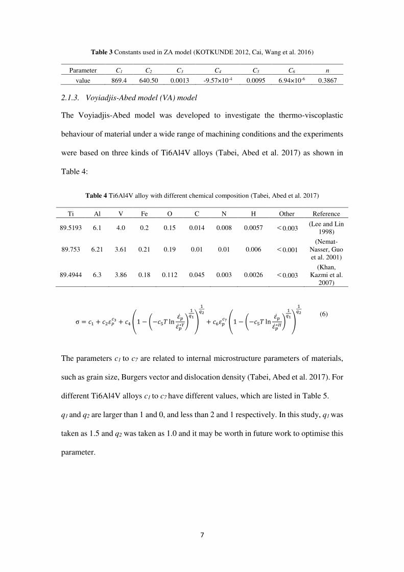
2.1.3. Voyiadjis-Abed model (VA) model
The Voyiadjis-Abed model was developed to investigate the thermo-viscoplastic
behaviour of material under a wide range of machining conditions and the experiments
were based on three kinds of Ti6Al4V alloys (Tabei, Abed et al. 2017) as shown in
Table 4:
Table 4 Ti6Al4V alloy with different chemical composition (Tabei, Abed et al. 2017)
Ti Al V Fe O C N H Other Reference
89.5193 6.1 4.0 0.2 0.15 0.014 0.008 0.0057 <0.003 (Lee and Lin
1998)
89.753 6.21 3.61 0.21 0.19 0.01 0.01 0.006 <0.001 (Nemat-
Nasser, Guo et al. 2001)
89.4944 6.3 3.86 0.18 0.112 0.045 0.003 0.0026 <0.003 (Khan,
Kazmi et al. 2007)
σ = 𝑐1 + 𝑐2𝜀𝑃𝑐3 + 𝑐4 (1 − (−𝑐5𝑇 ln 𝜀�̇�𝜀�̇�∗𝑌) 1𝑞1) 1𝑞2 + 𝑐6𝜀𝑝𝑐7 (1 − (−𝑐5𝑇 ln 𝜀�̇�𝜀�̇�∗𝐻) 1𝑞1) 1𝑞2
(6)
The parameters c1 to c7 are related to internal microstructure parameters of materials,
such as grain size, Burgers vector and dislocation density (Tabei, Abed et al. 2017). For
different Ti6Al4V alloys c1 to c7 have different values, which are listed in Table 5.
q1 and q2 are larger than 1 and 0, and less than 2 and 1 respectively. In this study, q1 was
taken as 1.5 and q2 was taken as 1.0 and it may be worth in future work to optimise this
parameter.
8
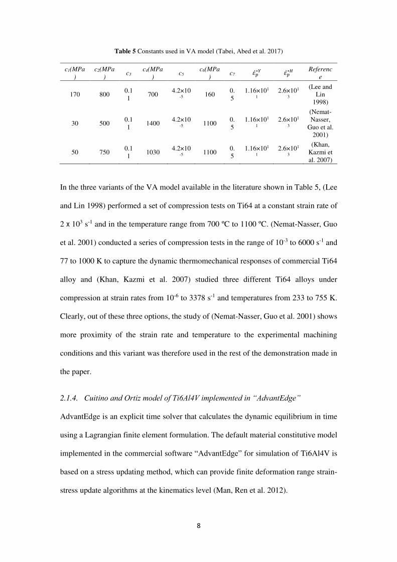
Table 5 Constants used in VA model (Tabei, Abed et al. 2017)
c1(MPa
)
c2(MPa
) c3
c4(MPa
) c5
c6(MPa
) c7 𝜀�̇�∗𝑌 𝜀�̇�∗𝐻
Referenc
e
170 800 0.11
700 4.2×10
-5 160
0.5
1.16×101
1 2.6×101
3
(Lee and Lin
1998)
30 500 0.11
1400 4.2×10
-5 1100
0.5
1.16×101
1 2.6×101
3
(Nemat-Nasser,
Guo et al. 2001)
50 750 0.11
1030 4.2×10
-5 1100
0.5
1.16×101
1 2.6×101
3
(Khan, Kazmi et al. 2007)
In the three variants of the VA model available in the literature shown in Table 5, (Lee
and Lin 1998) performed a set of compression tests on Ti64 at a constant strain rate of
2 х 103 s-1 and in the temperature range from 700 ºC to 1100 ºC. (Nemat-Nasser, Guo
et al. 2001) conducted a series of compression tests in the range of 10-3 to 6000 s-1 and
77 to 1000 K to capture the dynamic thermomechanical responses of commercial Ti64
alloy and (Khan, Kazmi et al. 2007) studied three different Ti64 alloys under
compression at strain rates from 10-6 to 3378 s-1 and temperatures from 233 to 755 K.
Clearly, out of these three options, the study of (Nemat-Nasser, Guo et al. 2001) shows
more proximity of the strain rate and temperature to the experimental machining
conditions and this variant was therefore used in the rest of the demonstration made in
the paper.
2.1.4. Cuitino and Ortiz model of Ti6Al4V implemented in “AdvantEdge”
AdvantEdge is an explicit time solver that calculates the dynamic equilibrium in time
using a Lagrangian finite element formulation. The default material constitutive model
implemented in the commercial software “AdvantEdge” for simulation of Ti6Al4V is
based on a stress updating method, which can provide finite deformation range strain-
stress update algorithms at the kinematics level (Man, Ren et al. 2012).

9
As per this model, the flow stress is defined as follows:
σ(α, 𝛼,̇ 𝑇) = g(𝛼)𝜃(𝑇)г(�̇�) (7)
where 𝑔(𝛼), 𝜃(𝑇) and г(�̇�) refer to the isotropic strain hardening function, thermal
softening and rate sensitivity respectively. The equations used to describe these three
parts are shown in (8), (9) and (10).
𝐺(𝛼) = σ0 (1 + 𝛼𝛼0)1𝑁 (8)
𝜃(𝑇) = 𝑐0 + 𝑐1𝑇 + ⋯ + 𝑐5𝑇5 (9)
г(�̇�) = (1 + �̇��̇�0) 1𝑀
(10)
where 𝜎0 refers to the initial yield stress, 𝛼0 represents the reference strain and �̇�0 is
reference strain rate.
2.1.5. Tabulated flow stress model of Ti6Al4V implemented in “DEFORM”
DEFORM is an Implicit solver employing the Newton Raphson technique. The default
material model of Ti6Al4V used in DEFORM follows an equation 𝜎 = 𝜎(𝜀,̅ 𝜀̇, 𝑇),
where 𝜎, 𝜀,̅ 𝜀̇ and T refer to flow stress, equivalent plastic strain, equivalent plastic
strain rate and temperature respectively. In order to reflect the true material behaviour
of Ti6Al4V, the data of these parameters at several data point are fed using a tabular
data format and a linear weighted average interpolation method is used to calculate the
data at unknown points between existing flow stress data points. The stress-strain curve
based on this tabulated model is shown in Fig. 1.

10
Fig. 1. Tabulated flow stress model of Ti6Al4V
3. FEA methodology
In order to perform the FEA simulation, a VUMAT code in Abaqus was developed so
that each of the aforementioned material models can readily be described to study the
material behaviour of Ti6Al4V. The idea was to first compare the VUMAT results
against the standard results predicted by the software for a typical material model like
the JC model, which is readily available in every software and thus, the VUMAT sub-
routine validity and reliability was established. The process to call the code in Abaqus
followed the flowchart shown in Fig. 2.

11
Fig. 2. Flowchart of calling VUMAT in Abaqus as implemented in this work
3.1. Tensile testing
3.1.1. Testing considerations
Prior to performing the FEA analysis on Ti6Al4V, we benchmarked our model by
comparing uniaxial tensile test stress-strain plots using the same VUMAT sub-routine
but merely by changing the parameters to be for silicon instead of Ti6Al4V. The same
conditions and material constants were used to reproduce the strain-stress curve. This
step helped us validate the results against the previously published paper by the authors
of this paper (Goel, Llavori et al. 2018). It may be noted that the microscale and
nanoscale properties are affected by the so called “size effect” and hence they cannot
be extrapolated readily but the idea to simulate the nanoscale tensile test is merely to
benchmark the model.
Accordingly, the work began by first performing the tensile test on silicon using the
built-in JC model provided by Abaqus as a default choice and it was then compared
with the tensile test of silicon using VUMAT code. The material properties used to
Input material constants, current stress, and strain
increment
Calculate the trial stress
Calculate the hydrostatic stress,
deviatoric stress and von mises stress
Yielding occur
Update stress, strain, energy
End and go back to main routine
Start Bisection iteration method to find the
real equivalent plastic strain
increment
Calculate the true stress
Accumulate the damage factor w
Damage initiation
occur
Accumulate the stiffness degradation
factor D
Fully degradation
Delete element
Yes
No
Yes
No
Yes
No

12
perform the simulation on silicon are listed in Table 6 while the material constants used
in the JC model are listed in Table 7.
Table 6 Material properties of silicon (Goel, Llavori et al. 2018)
Density(kg/m3) Poisson’s ratio Elastic modulus (GPa)
2330 0.23 98
Table 7 Constants used in JC model for silicon (Goel, Llavori et al. 2018)
A (MPa) B (MPa) N m C 𝜀0̇(s-1) Troom (K) Tmelt (K)
896.394 529.273 0.3758 1 0.4242 1 293 1688
3.1.2. Boundary conditions and model development
As for the tensile testing, a cylindrical workpiece of diameter 20.68 nm and length 48.98
nm was used to maintain the traceability with the literature (Goel, Llavori et al. 2018).
Fig. 3. FEA model of the workpiece
A 10-node modified quadratic tetrahedron (C3D10M) element was used in this study
and dynamic explicit analysis was chosen. As Fig.3 shows (on the left), the displacement
in the z direction was restricted and therefore the transverse contraction of the
workpiece was allowed in both the x and y direction. On the right side, the velocity load
was applied. In order to research the effect of different strain rates, the test strain rate
was taken in the range of 1×10⁻³/ps to 1×10⁻⁵/ps according to the recent paper
researching nanoscale tensile testing (Zhang, Han et al. 2007). The strain rate was
converted into an equivalent velocity in order to define the appropriate boundary
condition as follows:

13
𝜀̇ = 𝜀𝛥𝑡 = 𝛥𝑙𝑙0𝛥𝑡 = 𝜈𝑙0 (11) 𝜈 = 𝑙0 × 𝜀̇ = 48.98 × 10−6 × 5 × 108 = 24490 𝑚𝑚/𝑠 (12)
where 𝜈 is equivalent velocity, l0 is the initial length of the objective workpiece, 𝛥𝑙 is
the change of length. When the length l0 was taken as 48.98 nm (48.98×10⁻⁹ m) and
strain rate 𝜀̇ was taken as 0.0005/ps (5×10⁸ s), a fixed velocity load 24490 mm/s was
applied on the workpiece during the simulation. A good overlap (shown in the later
section) was found confirming reliability of the model.
Table 8 Material properties of Ti6Al4V (Gu, Dong et al. 2015)
Density(kg/m3) Poisson’s ratio Elastic modulus (GPa)
4430 0.33 110
Table 9 Constants used in different models (Gu, Dong et al. 2015)
After performing a satisfactory comparison for silicon, the material description was
changed from silicon to Ti6Al4V and this way a well calibrated tensile testing model
Model Parameter Reference
ZA
C1 C2 C3 C4 C5
(KOTKUNDE 2012)
869.4 640.50 0.0013 -9.57×10⁻⁴ 0.0095
C6 N
6.94×10⁻⁶ 0.3867
VA
C1 (MPa) C2(MPa) C3 C4 (MPa) C5
(Tabei, Abed et al. 2017)
30 500 0.11 1400 4.2×10⁻⁵
C6(MPa) C7 𝜀�̇�∗𝑌 𝜀�̇�∗𝐻
1100 0.5 1.16×10¹¹ 2.6×10¹³
JC-1
A (MPa) B (MPa) N m C
(KOTKUNDE 2012)
896.4 649.5 0.3867 0.7579 0.0093 𝜀0̇(s-1) Tref (K) Tmelt (K)
1 323 1923
JC-2
A (MPa) B (MPa) N m C
(Gu, Dong et al. 2015)
1098 1092 0.93 1.1 0.014 𝜀0̇(s-1) Tref (K) Tmelt (K)
1 298 1878
14
was obtained for Ti6Al4V. We then performed the predictive work via this model to
compare the different material models under uniaxial stress conditions as well as to
probe the influence of the strain rate effects on the resulting stress-strain plots. The
material properties and other constants used to perform the tensile test simulation on
Ti6Al4V using JC, ZA and VA models are shown in Table 8 and Table 9.
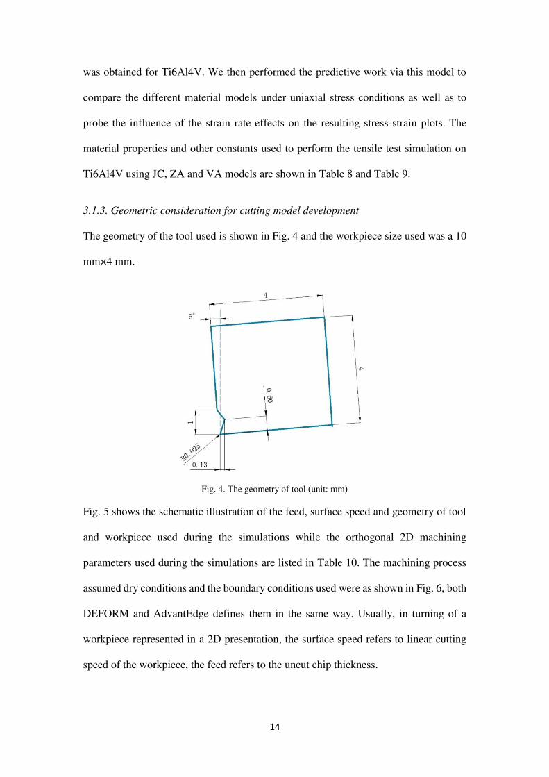
3.1.3. Geometric consideration for cutting model development
The geometry of the tool used is shown in Fig. 4 and the workpiece size used was a 10
mm×4 mm.
Fig. 4. The geometry of tool (unit: mm)
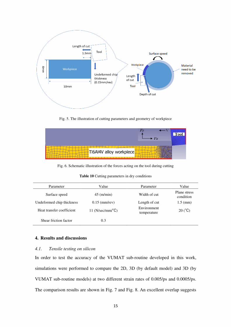
Fig. 5 shows the schematic illustration of the feed, surface speed and geometry of tool
and workpiece used during the simulations while the orthogonal 2D machining
parameters used during the simulations are listed in Table 10. The machining process
assumed dry conditions and the boundary conditions used were as shown in Fig. 6, both
DEFORM and AdvantEdge defines them in the same way. Usually, in turning of a
workpiece represented in a 2D presentation, the surface speed refers to linear cutting
speed of the workpiece, the feed refers to the uncut chip thickness.
15
Fig. 5. The illustration of cutting parameters and geometry of workpiece
Fig. 6. Schematic illustration of the forces acting on the tool during cutting
Table 10 Cutting parameters in dry conditions
Parameter Value Parameter Value
Surface speed 45 (m/min) Width of cut Plane stress condition
Undeformed chip thickness 0.15 (mm/rev) Length of cut 1.5 (mm)
Heat transfer coefficient 11 (N/sec/mm/℃) Environment temperature 20 (℃)
Shear friction factor 0.3
4. Results and discussions
4.1. Tensile testing on silicon
In order to test the accuracy of the VUMAT sub-routine developed in this work,
simulations were performed to compare the 2D, 3D (by default model) and 3D (by
VUMAT sub-routine models) at two different strain rates of 0.005/ps and 0.0005/ps.
The comparison results are shown in Fig. 7 and Fig. 8. An excellent overlap suggests

16
that the developed VUMAT worked well on silicon and thus became the basis for
testing various material models of Ti6Al4V in the next section.
Fig. 7. Comparison between built-in model and VUMAT subroutine (0.005/ps)
Fig. 8. Comparison between built-in model and VUMAT subroutine (0.0005/ps)
0
1
2
3
4
5
6
7
8
9
10
11
12
0 0.01 0.02 0.03 0.04 0.05 0.06 0.07 0.08 0.09 0.1 0.11 0.12 0.13 0.14
Tru
e s
tre
ss (
GP
a)
Strain
Stress-strain curve (0.005/ps)
2D FEA result
3D FEA result
3D FEA result (VUMAT)
0
1
2
3
4
5
6
7
8
9
10
11
0 0.01 0.02 0.03 0.04 0.05 0.06 0.07 0.08 0.09 0.1 0.11 0.12 0.13 0.14
Tru
e s
tre
ss (
GP
a)
Strain
Stress-strain curve (0.0005/ps)
2D FEA result
3D FEA result
3D FEA result (VUMAT)
17
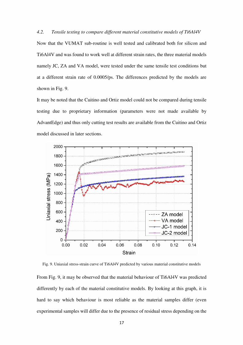
4.2. Tensile testing to compare different material constitutive models of Ti6Al4V
Now that the VUMAT sub-routine is well tested and calibrated both for silicon and
Ti6Al4V and was found to work well at different strain rates, the three material models
namely JC, ZA and VA model, were tested under the same tensile test conditions but
at a different strain rate of 0.0005/ps. The differences predicted by the models are
shown in Fig. 9.
It may be noted that the Cuitino and Ortiz model could not be compared during tensile
testing due to proprietary information (parameters were not made available by
AdvantEdge) and thus only cutting test results are available from the Cuitino and Ortiz
model discussed in later sections.
Fig. 9. Uniaxial stress-strain curve of Ti6Al4V predicted by various material constitutive models
From Fig. 9, it may be observed that the material behaviour of Ti6Al4V was predicted
differently by each of the material constitutive models. By looking at this graph, it is
hard to say which behaviour is most reliable as the material samples differ (even
experimental samples will differ due to the presence of residual stress depending on the

18
processing history) but Fig. 9 mainly highlights the extent of differences between these
various material models. The nanoscale yield stress of Ti6Al4V, revealed by the ZA,
VA, JC-1, JC-2 models were 1531.03 MPa, 1455.71 MPa, 1077.55 MPa, 1234.54 MPa
respectively. The variations in the subsequent plastic behaviour are well evident. One
may note here that the JC-2 model was developed at room temperature (25 ºC) while
the JC-1 model was developed at a slightly higher temperature (50 ºC). Interestingly,
the VA model showed more noise whilst the other three models provided a smoother
plot.
4.3. Tensile testing on Ti6Al4V at different strain rates using JC-2 model
This section shows the effect of strain rate on Ti6Al4V using JC-2 model while varying
the strain rates between 0.001/ps, to 0.00001/ps (see fig 10). At higher strain rates, the
value of stress was observed to be higher. It signified that the strain rate has a marked
influence on the plastic response of Ti6Al4V especially in the deformation zone i.e.
higher strain rate was accompanied by an increase in the strain energy absorbed by
Ti6Al4V before rupture. The slope of the linear curve in the elastic regime refers to
elastic modulus of the material, here obtained as 110 GPa for Ti6Al4V.
Fig. 10. The influence of strain rate on the uniaxial stress-strain behaviour of Ti6Al4V
00.10.20.30.40.50.60.70.80.9
11.11.21.31.41.51.61.7
0.00 0.01 0.02 0.03 0.04 0.05 0.06 0.07 0.08 0.09 0.10 0.11 0.12 0.13 0.14
Str
ess
(GP
a)
Strain
Stress-strain (Built-in model)
0.001/ps
0.0005/ps
0.0001/ps
0.00005/ps
0.00001/ps

19
4.4. Cutting test simulations
4.4.1 Stress and temperature
A snapshot captured from the cutting simulations of Ti6Al4V while using the same
cutting parameters but different material constitutive equations, namely the tabulated
stress model (used as benchmark) compared with the JC-1, JC-2, ZA and Cuitino and
Ortiz models (obtained from AdvantEdge) - see Fig 11 to Fig 15. These cutting
simulations assumed an uncoated carbide cutting tool to investigate stress and
temperature in the cutting zone during the machining process.
Fig. 11. The effective stress and temperature during machining process obtained from DEFORM using
tabulated stress model (benchmark)
Fig. 12. The effective stress and temperature obtained from DEFORM using JC-1 model

20
Fig. 13.The effective stress and temperature obtained from DEFORM using JC-2 model
Fig. 14. The effective stress and temperature obtained from DEFORM using ZA model
Fig. 15. The effective stress and temperature obtained from AdvantEdge using Cuitino and Ortiz model

21
Table 11 Summary of cutting results showing stress and temperature peak in the cutting zone of Ti6Al4V
obtained from the simulations
Material model name Peak stress (MPa) in the cutting
zone of Ti6Al4V Peak temperature (°C) in the
cutting zone of Ti6Al4V
Tabulated stress model (Benchmark)
1470 641
JC-1 1190 570
JC-2 1400 800
ZA model 1710 917
Cuitino and Ortiz model (obtained from AdvantEdge)
1600 600
A summary of the results obtained from different models highlighting peak stress and
temperature is provided in Table 11. Similar to the observations noted from the uniaxial
stress test, the peak von Mises stress in the cutting zone of Ti6Al4V was seen as
consistent with the peak uniaxial stress. Most of these results suggest that the ZA model
predicts the peak temperature and peak temperature in the cutting zone as much higher
than the predictions made by the other models, while the JC-1 model underestimates
these. In general, the peak maximum stress during cutting of Ti6Al4V was about 1470
MPa while the peak machining temperature in the cutting zone was of the order of 600
ºC.
The chip morphology observed in the simulations showed the Saw-tooth chip
characteristic which is unique to Ti6Al4V and many reports are published in the
literature verifying the simulation based observations reported in this work (Gente,
Hoffmeister et al. 2001, Hua and Shivpuri 2004, Calamaz, Coupard et al. 2008). The
cutting chips are widely recognised as being the fingerprint of the metal machining
process and are broadly classified in two categories: steady state continuous chips and
cyclic chips (Saw-tooth chips are one kind of cyclic chip) (Vyas and Shaw 1999).
Extant literature on the formation of Saw-tooth chips (as evidenced by the FEA
simulations in this work while cutting Ti6Al4V) proposes two broad theories (i)

22
adiabatic shear theory and (ii) cyclic crack theory (Calamaz, Coupard et al. 2011). A
new theory combining both of these was also proposed and Saw-tooth chip formation
is said to be due to adiabatic shear sensitivity of the material i.e. Saw-tooth chips of
sensitive materials are formed due to thermoplastic instability whereas chips of
insensitive materials are formed due to crack initiation and propagation (Upadhyay,
Jain et al.). The chip morphology could be affected by many factors, such as cutting
parameters, mechanical properties (Fu, Chen et al. 2017), and material constitutive
models. The cutting speed and feed rate had the opposite effect on Saw-tooth chip
morphology. While an increase in cutting speed reduces the peak height of Saw-tooth
chips, a higher feed rate increases this peak height (Bai, Sun et al. 2017). The material
constitutive models influence thermoplastic shear as well as the hot mechanical
properties. From the results shown in Table 11, it may be seen that high temperature is
accompanied by an increased cutting force indicating that work hardening is less
influential at temperatures around 900 ºC. Meanwhile, when plastic strain reached a
critical value, a shear band was formed and the chip segmentation occurred, so the
periodic shear bands were observed in the FEA to be due to the periodic nature of this
cycle resulting in the Saw-tooth chip-formation process, causing fluctuations in the
force curve (Bai, Sun et al. 2017).
4.4.2. Variation in the forces during cutting
The simulation results were used to extract the cutting forces in the two principal
directions, Fc or Fx acting in the X direction (shown earlier in Figure 6) referred to as
axial cutting force or feed force in machining context or a friction force during a normal
scratch test whilst Ft or acts in the Y direction referred to as tangential cutting force or
thrust force in machining and as normal force in the scratching literature. The ratio of
Fx/Fy (friction force/normal force) during cutting is referred to as “coefficient of kinetic

23
friction” (COF) and is a useful indicator to compare simulation against experiments
(Goel, Stukowski et al. 2013). A comparison of results obtained for Fx and Fy is shown
in Fig. 16 and Fig. 17. As it may be seen, the JC-2 model showed the closest proximity
with the tabulated stress model in comparison to the JC-1 model. Also, the Cuitino and
Ortiz model results extracted from AdvantEdge showed wide fluctuations and larger
values of forces compared to the other three models. It is obvious that the forces are
much higher in the case of AdvantEdge.
Fig. 16. Comparison of cutting force in x direction
Fig. 17. Comparison of cutting force in y direction
-200
-100
0
100
200
300
400
500
600
700
0 0.2 0.4 0.6 0.8 1 1.2 1.4 1.6
Cut
ting
for
ce (
N)
Length of cut (mm)
Cutting force in X direction
Cuitino Ortiz (Fx) JC-1 (Fx) JC-2 (Fx) Benckmark (Fx) ZA (Fx)
-200
-100
0
100
200
300
400
500
0 0.2 0.4 0.6 0.8 1 1.2 1.4 1.6
Cut
ting
for
ce (
N)
Length of cut (mm)
Cutting force in Y direction
Cuitino Oritz (Fy) JC-1 (Fy) JC-2 (Fy) Benckmark (Fy) ZA (Fy)

24
Table 12 Simulation results comparing various material models tested in this work
A summary of these results is presented in Table 12 showing quantitative differences
in the forces revealed by the material models. At this point, it becomes an intellectual
curiosity to survey the literature to see how the values of COF obtained from the
simulations in this work compare with the literature. In that spirit, several papers were
reviewed from the literature which have looked at machining Ti6Al4V both using
simulations and experiments and the values of COF were extracted to compare with the
current simulations shown in Figure 18.
Figure 18: Comparison of simulation wise obtained values of COF against the surveyed
wealth of literature reporting various values of COF as a function of cutting speed
Material
Model
Friction
force (Fx)
(N)
Percentage
difference
(%)
Thrust
force (Fy)
(N)
Percentage
difference
(%)
COF
(Fx/Fy)
Percentage
difference
(%)
Tabulated
flow stress
(Benchmark)
219.1486 64.3060 3.4079
JC-1 166.7175 23.9 42.9255 33.2 3.8839 -14.0
JC-2 212.875 2.9 62.5376 2.8 3.4040 0.1
ZA 185.4594 15.4 66.6738 -3.7 2.7816 18.4
Cuitino Ortiz 298.812 -36.4 150.147 -133.5 1.9901 41.6
25
In preparation of Figure 18 the works reviewed were that of (Dorlin, Fromentin et al.
2016), (Bahi, List et al. 2016), (Bai, Sun et al. 2017), (Li, Qiu et al. 2016), (Ruibin and
Wu 2016), (Shalaby and Veldhuis 2018) and (Vosough, Schultheiss et al. 2013). There
are a number of other works reported on machining Ti6Al4V but we draw this brief
comparison merely for the purpose of comparing the results we obtained from our
models rather than consolidating the entire series of experimental trials performed on
Ti6Al4V to date. From Figure 18, it is evident that the COF during machining of
Ti6Al4V is larger than unity i.e. friction force is higher than the thrust force. It was,
however, not immediately clear from this comparison to say which model makes the
best prediction. We however note that the work of (Vosough, Schultheiss et al. 2013)
has an inherent advantage for comparing the results reported in the simulation study
presented here. They compared their experimental results readily against the JC model
and obtained very close proximity between their simulations and experiments. It
alluded to the fact that the proposed benchmarked tabulated stress model and the JC-2
model performed fairly consistently with their reported experimental results.
4.5. Comparison of peak stress during tensile testing and during cutting
As a final step, a comparison was made to examine the peak stress obtained from the
tensile test and von Mises equivalent stress obtained during machining (see Table 13).
This comparison shows that the von Mises flow (deviatoric strain energy or J2 theory)
criterion in a ductile metal like Ti6Al4V follows the uniaxial stress consistently across
all the material models tested in the work. Also, if the tabulated material model is to be
considered as a good benchmark then the JC-2 model seems to be a more consistent
model in predicting the material response of Ti6Al4V under a wide variety of stress
behaviours during tribology, wear, machining and other contact loading conditions.
This observation is also supported by the work of (Vosough, Schultheiss et al. 2013)

26
who have validated the JC-2 model for a wide range of uncut chip thicknesses with
their experiments on Ti alloy.
Table 13 Comparison of flow stress of different testing with different models
Model
Tensile testing Cutting
Uniaxial (true)
stress (MPa)
Percentage
difference (%)
von Mises stress
(MPa)
Percentage
difference (%)
Tabulated flow
stress model of
Deform
/ / 1470 0
JC-1 model 1180 19.7 1190 19.0
JC-2 model 1420 3.4 1400 4.8
ZA model 1670 -13.6 1710 -16.3
Cuitino Ortiz 1600 -8.8
5. Conclusions
This paper aims to elucidate quantifiable differences between a wide range of material
constitutive models available for simulation of the important biomaterial and aerospace
material Ti6Al4V. In the past, more than a dozen material models have been proposed
(e.g. the Arrhenius-Type model, the Field-Backofen model, the Khan-Huang-Liang
model, the Mechanical Threshold Stress model, the Johnson-Cook model, the Multi-
Branch model, the Tangent hyperbolic model, the Voyiadjis-Abed model, the Zerilli-
Armstrong (ZA) model, the Baker Modification of the EI-Magd model, the Cuitino and
Ortiz model and the tabulated material model) to perform finite element analysis of
contact loading simulations on Ti6Al4V alloys. Several of these material models are
widely used and implemented commercially, such as the Johnson-cook model,
tabulated flow stress model and ZA model.
Taking the examples of a uniaxial tensile test and cutting tests, these models were
compared to draw a quantifiable comparison. This study in its present form will help
researchers in addressing more specific engineering issues like wear, tribology and

27
contact loading which are critical for delicate biomedical applications. From the various
simulation test cases performed and reported in this study, the following may be
concluded:
(i) Strain rate has a marked influence on the plastic response of Ti6Al4V especially in
the deformation zone i.e. within the range of strain rates tested, higher strain rate was
accompanied by an increase in the strain energy absorbed by Ti6Al4V before rupture.
(ii) Across various material models reported in the literature, one variant of the
Johnson-Cook model seems to provide the most consistent values for the uniaxial
tensile simulations and scratch tests. As is known for macroscopic cutting, the friction
force (Fx) was observed to be higher than the normal force (Fy) during cutting of
Ti6Al4V. The coefficient of kinetic friction reported in the literature during various
cutting tests varies so widely that makes it difficult to say which particular material
model will be the best for a given material. However, the results compared to the
tabulated flow stress model used as a benchmark showed a proximity within an error
of 5% in predicting the peak von Mises stress and cutting forces obtained from the JC-
2 model as opposed to other material models that showed variations beyond 40% in the
cutting force predictions and up to 20% in estimating the peak stress in the cutting zone.
(iii) All material models revealed the phenomenon of Saw-tooth kind of chips being the
characteristic feature of Ti6Al4V deformation during scratching. Moreover, the
instantaneous change in the friction force reflected the process of chip formation i.e. an
increase in the friction force reflected the deformation occurring in the area of contact
between the cutter’s attack angle causing a shear slip when the stress reached beyond a
threshold value. The cycle repeats, and this leads to periodic formation of the chips

28
which appears to be like Saw-tooth chips. In the past this has been proposed to be due
to the adiabatic shear and subsequent crack initiation.
(iv) The cutting forces extracted from two commercial softwares (i.e. DEFORM-2D
and AdvantEdge) were found to be different and incomparable not just due to the way
the two different material models are implemented but also the way in which the
numerical calculations are performed in estimating the cutting forces, stresses and
temperature. In particular, AdvantEdge calculates the dynamic equilibrium in time by
an explicit time integration method using a Lagrangian finite element formulation
whilst DEFORM is an Implicit solver employing the Newton Raphson technique.
Acknowledgements:
This work was motivated by the necessity to understand material models to enable
working on grants supported by various funders, such as the RCUK (Grant No.
EP/S013652/1), H2020 (EURAMET EMPIR A185 (2018)) and Royal Academy of
Engineering (Grant No. IAPP18-19\295). The work was carried out in the Centre for
Doctoral Training in Ultra-Precision at Cranfield University which is supported by the
RCUK via Grants No.: EP/K503241/1 and EP/L016567/1. CL is deeply indebted to the
financial support from China Scholarship Council and AECC as well as the technical
inputs from Dr Ravi Kant (IIT Ropar), Dr Gasser Abdelal (QUB, Belfast) and Dr Ping
Zhou (Dalian, China). Part of this work used ARCHER UK National Supercomputing
Service (http://www.archer.ac.uk).
References
Alvarez, R., R. Domingo and M. A. Sebastian (2011). "The formation of saw toothed chip in a titanium alloy: influence of constitutive models." Strojniški vestnik-Journal of Mechanical Engineering 57(10): 739-749. Bahi, S., G. List and G. Sutter (2016). "Modeling of friction along the tool-chip interface in Ti6Al4V alloy cutting." The International Journal of Advanced Manufacturing Technology 84(9-12): 1821-1839.

29
Bai, W., R. Sun, A. Roy and V. V. Silberschmidt (2017). "Improved analytical prediction of chip formation in orthogonal cutting of titanium alloy Ti6Al4V." International Journal of Mechanical Sciences 133: 357-367. Cai, J., K. Wang and Y. Han (2016). A Comparative Study on Johnson Cook, Modified Zerilli–Armstrong and Arrhenius-Type Constitutive Models to Predict High-Temperature Flow Behavior of Ti–6Al–4V Alloy in α + β Phase. High Temperature Materials and Processes. 35: 297. Calamaz, M., D. Coupard and F. Girot (2008). "A new material model for 2D numerical simulation of serrated chip formation when machining titanium alloy Ti–6Al–4V." International Journal of Machine Tools and Manufacture 48(3-4): 275-288. Calamaz, M., D. Coupard, M. Nouari and F. Girot (2011). "Numerical analysis of chip formation and shear localisation processes in machining the Ti-6Al-4V titanium alloy." The International Journal of Advanced Manufacturing Technology 52(9-12): 887-895. Che, J., T. Zhou, Z. Liang, J. Wu and X. Wang (2018). "Serrated chip formation mechanism analysis using a modified model based on the material defect theory in machining Ti-6Al-4 V alloy." The International Journal of Advanced Manufacturing Technology 96(9-12): 3575-3584. Dorlin, T., G. Fromentin and J.-P. Costes (2016). "Generalised cutting force model including contact radius effect for turning operations on Ti6Al4V titanium alloy." The International Journal of Advanced Manufacturing Technology 86(9-12): 3297-3313. Fu, X., G. Chen, Q. Yang, Z. Sun and W. Zhou (2017). "The influence of hydrogen on chip formation in cutting Ti-6Al-4V alloys." The International Journal of Advanced Manufacturing Technology 89(1-4): 371-375. Gente, A., H.-W. Hoffmeister and C. Evans (2001). "Chip formation in machining Ti6Al4V at extremely high cutting speeds." CIRP Annals-Manufacturing Technology 50(1): 49-52. Goel, S., I. Llavori, A. Zabala, C. Giusca, S. C. Veldhuis and J. L. Endrino (2018). "The possibility of performing FEA analysis of a contact loading process fed by the MD simulation data." International Journal of Machine Tools and Manufacture 134: 79-80. Goel, S., A. Stukowski, X. Luo, A. Agrawal and R. L. Reuben (2013). "Anisotropy of single-crystal 3C–SiC during nanometric cutting." Modelling and Simulation in Materials Science and Engineering 21(6): 065004. Gu, X., C. Dong, J. Li, Z. Liu and J. Xu (2015). "MPM simulations of high-speed and ultra high-speed machining of titanium alloy (Ti–6Al–4V) based on fracture energy approach." Engineering Analysis with Boundary Elements 59: 129-143. Hua, J. and R. Shivpuri (2004). "Prediction of chip morphology and segmentation during the machining of titanium alloys." Journal of Materials Processing Technology 150(1-2): 124-133. Inagaki, I., T. Takechi, Y. Shirai and N. Ariyasu (2014). "Application and features of titanium for the aerospace industry." Nippon steel & sumitomo metal technical report 106: 22-27. Khan, A. S., R. Kazmi, B. Farrokh and M. Zupan (2007). "Effect of oxygen content and microstructure on the thermo-mechanical response of three Ti–6Al–4V alloys: experiments and modeling over a wide range of strain-rates and temperatures." International Journal of Plasticity 23(7): 1105-1125. Kotkunde, N., A. D. Deole, A. K. Gupta and S. K. Singh (2014). "Comparative study of constitutive modeling for Ti–6Al–4V alloy at low strain rates and elevated temperatures." Materials & Design 55: 999-1005.

30
KOTKUNDE, N. R. (2012). "Experimental and Numerical Investigations of Forming Behavior in Ti 6Al 4V Alloy at Elevated Temperatures." Lee, W.-S. and C.-F. Lin (1998). "High-temperature deformation behaviour of Ti6Al4V alloy evaluated by high strain-rate compression tests." Journal of Materials Processing Technology 75(1-3): 127-136. Leyens, C. and M. Peters (2003). Titanium and titanium alloys: fundamentals and applications, John Wiley & Sons. Li, P.-n., X.-y. Qiu, S.-w. Tang and L.-y. Tang (2016). "Study on dynamic characteristics of serrated chip formation for orthogonal turning Ti6Al4V." The International Journal of Advanced Manufacturing Technology 86(9-12): 3289-3296. Man, X., D. Ren, S. Usui, C. Johnson and T. D. Marusich (2012). "Validation of finite element cutting force prediction for end milling." Procedia CIRP 1: 663-668. Mosleh, A., A. Mikhaylovskaya, A. Kotov, T. Pourcelot, S. Aksenov, J. Kwame and V. Portnoy (2017). "Modelling of the Superplastic Deformation of the Near-α Titanium Alloy (Ti-2.5 Al-1.8 Mn) Using Arrhenius-Type Constitutive Model and Artificial Neural Network." Metals 7(12): 568. Nemat-Nasser, S., W.-G. Guo, V. F. Nesterenko, S. Indrakanti and Y.-B. Gu (2001). "Dynamic response of conventional and hot isostatically pressed Ti–6Al–4V alloys: experiments and modeling." Mechanics of Materials 33(8): 425-439. Özel, T. and Y. Karpat (2007). "Identification of constitutive material model parameters for high-strain rate metal cutting conditions using evolutionary computational algorithms." Materials and manufacturing processes 22(5): 659-667. Rashid, W. B., S. Goel, X. Luo and J. M. Ritchie (2013). "The development of a surface defect machining method for hard turning processes." Wear 302(1–2): 1124-1135. Ruibin, X. and H. Wu (2016). "Study on cutting mechanism of Ti6Al4V in ultra-precision machining." The International Journal of Advanced Manufacturing Technology 86(5): 1311-1317. Shalaby, M. A. and S. C. Veldhuis (2018). "Some observations on flood and dry finish turning of the Ti-6Al-4V aerospace alloy with carbide and PCD tools." The International Journal of Advanced Manufacturing Technology 99(9): 2939-2957. Tabei, A., F. Abed, G. Voyiadjis and H. Garmestani (2017). "Constitutive modeling of Ti-6Al-4V at a wide range of temperatures and strain rates." European Journal of Mechanics-A/Solids 63: 128-135. Upadhyay, V., P. Jain and N. Mehta "Comprehensive study of chip morphology in turning of Ti-6Al-4V." International Journal of Machining and Machinability of Materials 12: 358-371. Vosough, M., F. Schultheiss, M. Agmell and J.-E. Ståhl (2013). "A method for identification of geometrical tool changes during machining of titanium alloy Ti6Al4V." The International Journal of Advanced Manufacturing Technology 67(1): 339-348. Vyas, A. and M. Shaw (1999). "Mechanics of saw-tooth chip formation in metal cutting." Journal of Manufacturing Science and Engineering 121(2): 163-172. Xiulin, S., Z. Shiguang, G. Yang and C. Bin (2015). 3-D Finite Element Simulation Analysis of Milling Titanium Alloy Using Different Cutting Edge Radius. 2015 Sixth International Conference on Intelligent Systems Design and Engineering Applications (ISDEA), IEEE. Yadav, A. K., V. Bajpai, N. K. Singh and R. K. Singh (2017). "FE modeling of burr size in high-speed micro-milling of Ti6Al4V." Precision Engineering 49: 287-292.

31
Yameogo, D., B. Haddag, H. Makich and M. Nouari (2017). "Prediction of the cutting forces and chip morphology when machining the Ti6Al4V alloy using a microstructural coupled model." Procedia CIRP 58: 335-340. Zhang, Y., X. Han, K. Zheng, Z. Zhang, X. Zhang, J. Fu, Y. Ji, Y.-j. Hao, X.-y. Guo and Z. Wang (2007). "Direct observation of super‐plasticity of beta‐SiC nanowires at low temperature." Advanced Functional Materials 17(17): 3435-3440.