benchmarking the collocation stand- alone library … · benchmarking the collocation stand-alone...

BENCHMARKING THE COLLOCATION STAND-

ALONE LIBRARY AND TOOLKIT (CSALT)STEVEN HUGHES*

JEREMY KNITTEL*

WENDY SHOAN*

YOUNGKWANG KIM+

CLAIRE CONWAY^

DARREL CONWAY^

INTERNATIONAL SYMPOSIUM ON SPACE FLIGHT DYNAMICS

JUNE 8TH, 2017

*+ ^

https://ntrs.nasa.gov/search.jsp?R=20170005482 2020-03-23T05:53:48+00:00Z

AGENDA

Motivation

Optimal Control Problems

CSALT

General Optimal Control Benchmarking Results

Low-Thrust Trajectory Design Benchmarking Results

Summary/Future Work

MOTIVATION

Physical systems which involve time varying control decisions can rarely be solved analytically

Low-thrust spacecraft trajectories cannot be designed using intuition

NASA Goddard’s General Mission Analysis Toolkit (GMAT) has limited capability to solve low-thrust

problems

Goals:

Demonstrate that CSALT can solve industry-standard optimal control problems

Demonstrate that CSALT can solve optimal control low-thrust trajectory problems

Compare CSALT execution efficiency to other optimal control software packages

AGENDA

Motivation


CSALT



Summary/Future Work

OPTIMAL CONTROL PROBLEMS

Minimize a cost function of the form:

Subject to the following set of ordinary differential equations:

Subject to algebraic path constraints:

Subject to boundary conditions:

AGENDA

Motivation


CSALT



Summary/Future Work

COLLOCATION STAND-ALONE LIBRARY AND TOOLKIT

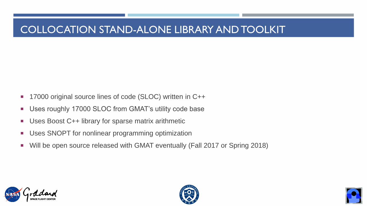
17000 original source lines of code (SLOC) written in C++

Uses roughly 17000 SLOC from GMAT’s utility code base

Uses Boost C++ library for sparse matrix arithmetic

Uses SNOPT for nonlinear programming optimization

Will be open source released with GMAT eventually (Fall 2017 or Spring 2018)

CURRENT CSALT CAPABILITY

Multiple collocation transcriptions

Trapezoid

Hermite-Simpson

Lobatto IIIa of order 4,6 and 8

Radau Orthagonal

Multiple cost-function formulations

Mayer

Lagrange

Bolza

Algebraic path and point constraints

Decision vector, cost and constraint scaling

Analytical collocation derivatives with finite differenced user point and path functions

Automatic sparsity pattern determination

Mesh refinement (Radau transcription only)

AGENDA

Motivation


CSALT



Summary/Future Work

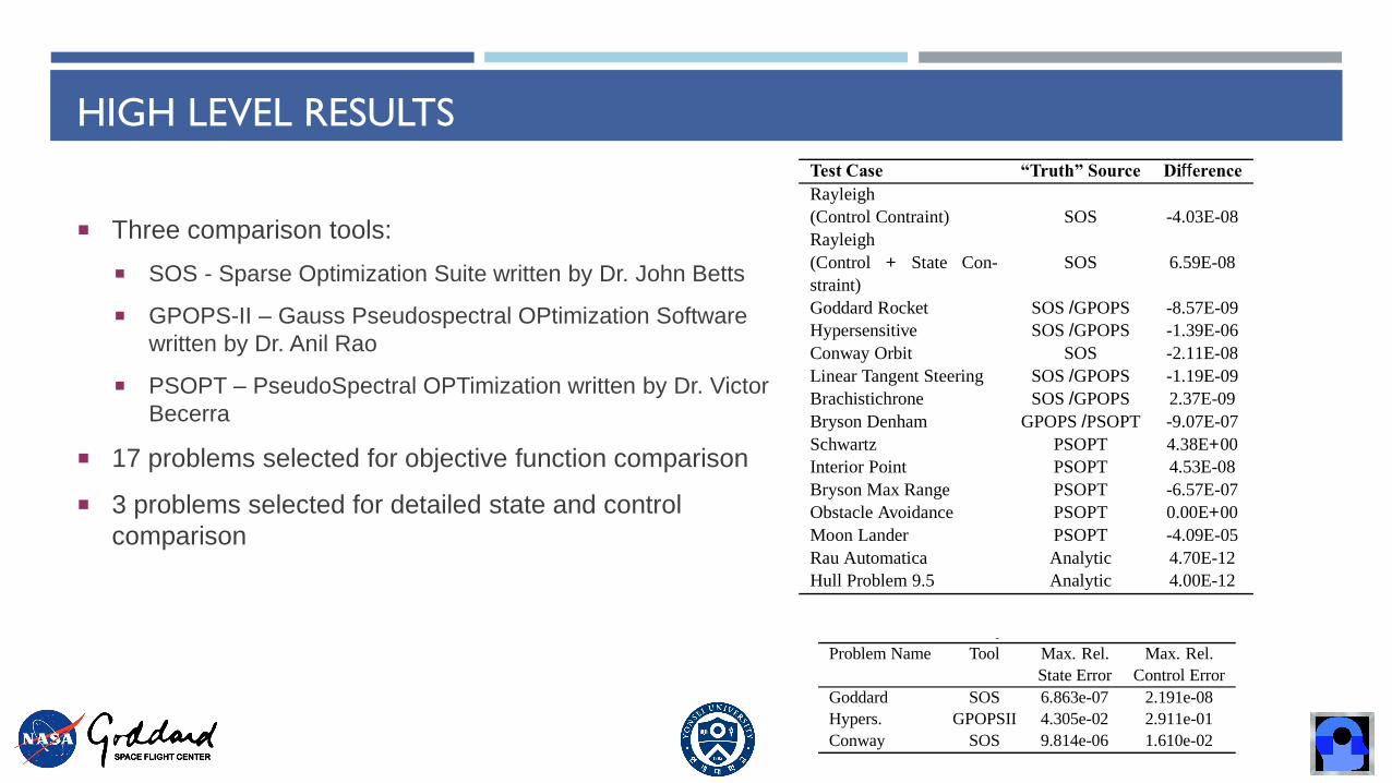
HIGH LEVEL RESULTSTable 2. High level optimal control comparisons

Test Case “Truth” Source Difference

Rayleigh

(Control Contraint) SOS -4.03E-08

Rayleigh

(Control + State Con-

straint)

SOS 6.59E-08

Goddard Rocket SOS /GPOPS -8.57E-09

Hypersensitive SOS /GPOPS -1.39E-06

Conway Orbit SOS -2.11E-08

Linear Tangent Steering SOS /GPOPS -1.19E-09

Brachistichrone SOS /GPOPS 2.37E-09

Bryson Denham GPOPS /PSOPT -9.07E-07

Schwartz PSOPT 4.38E+00

Interior Point PSOPT 4.53E-08

Bryson Max Range PSOPT -6.57E-07

Obstacle Avoidance PSOPT 0.00E+00

Moon Lander PSOPT -4.09E-05

Rau Automatica Analytic 4.70E-12

Hull Problem 9.5 Analytic 4.00E-12

Table 3. CSALT Comparison to Exact Solutions

Problem Max. State Error Max. Control Error

Hull Problem 9.5 2.876e-09 2.817e-08

Rao Automatica 5.109e-08 2.391e-06

0 0.5 1 1.5 2

Time, non-dim.

0

1

2

Sta

te,

no

n-d

im.

CSALT

Exact

0 0.5 1 1.5 2

Time, non-dim.

0

0.5

1

Co

ntr

ol, n

on

-dim

.

CSALT

Exact

Fig. 1. State and Control Comparison for Rao Automatica

control differences between CSALT and the solution generated

by either SOS or GPOPSII. Note, comparison of the cost solu-

tion was discussed in the problem overview section.

Figures 2 and 3 show relevant portions of the state and con-

trol history for the Hypersensitive orbit problem computed by

CSALT and GPOPSII. For the hypersensitive problem, the dy-

namics change rapidly at the beginning and end of the time

window, and are nearly constant for the middle portions of the

window and the solutions between CSALT and GPOPSII are

similar. Table 4 shows the maximum relative state and control

difference of 4.305e-02 and 2.911e-01 respectively. These are

larger than desirable. We believe the difference is due to inter-

polation to common discretization times and this is supported

by comparing the agreement between SOS and GPOPS-II solu-

tions where the maximum relative state and control differences

are 3.54e-01 and 1.037 respectively when interpolated to com-

mon discretization times using cubic splines.

0 5 10 15 20 25

Time, Non-Dim.

0

0.5

1

Sta

te,

No

n-D

im.

CSALT

GPOPSII

Fig. 2. State Comparison for Hypersensitive Problem

0 10 20 30

Time, Non-Dim.

-0.4

-0.3

-0.2

-0.1

0

Co

ntr

ol N

on

-Dim

.

CSALT

GPOPSII

Fig. 3. Control Comparison for Hypersensitive Problem

Figures 4 and 5 show the state and control history for the

Conway orbit problem computed by CSALT and SOS. The

problem is a finite thrust orbit raising problem, and the solu-

tion results in three orbital revolutions. The solutions are qual-

itatively similar and differences cannot be seen on the scale of

the graphics. Table 4 contains data illustrating the maximum

state and control differences between the two systems. The

state agreement is excellent with a maximum relative difference

of 9.814e-06, while the maximum relative control difference is

1.610e-02.

The state and control histories for the Goddard Rocket Prob-

lem from CSALT and SOS are shown in Figures 6-8. The prob-

lem contains three phases and the solutions are qualitatively

consistent. The control is discontinuous and has a bang-off

structure for the first and third phase, and in the second phase

thrust is varied to maintain terminal velocity (in the upward di-

rection!). The maximum relative difference for state and control

agreement is excellent, with maximum differences of 6.863e-07

and 2.191e-08, respectively.

Table 4. CSALT Comparison to Other Collocation Tools

Problem Name Tool Max. Rel. Max. Rel.

State Error Control Error

Goddard SOS 6.863e-07 2.191e-08

Hypers. GPOPSII 4.305e-02 2.911e-01

Conway SOS 9.814e-06 1.610e-02

4

Table 2. High level optimal control comparisons


Rayleigh


Rayleigh


straint)

SOS 6.59E-08
















Hull Problem 9.5 2.876e-09 2.817e-08


0 0.5 1 1.5 2

Time, non-dim.

0

1

2

Sta

te,

no

n-d

im.

CSALT

Exact

0 0.5 1 1.5 2

Time, non-dim.

0

0.5

1

Co

ntr

ol, n

on

-dim

.

CSALT

Exact



















0 5 10 15 20 25

Time, Non-Dim.

0

0.5

1

Sta

te,

No

n-D

im.

CSALT

GPOPSII


0 10 20 30

Time, Non-Dim.

-0.4

-0.3

-0.2

-0.1

0

Co

ntr

ol N

on

-Dim

.

CSALT

GPOPSII











1.610e-02.













Goddard SOS 6.863e-07 2.191e-08


Conway SOS 9.814e-06 1.610e-02

4

Three comparison tools:

SOS - Sparse Optimization Suite written by Dr. John Betts

GPOPS-II – Gauss Pseudospectral OPtimization Software

written by Dr. Anil Rao

PSOPT – PseudoSpectral OPTimization written by Dr. Victor

Becerra

17 problems selected for objective function comparison

3 problems selected for detailed state and control

comparison

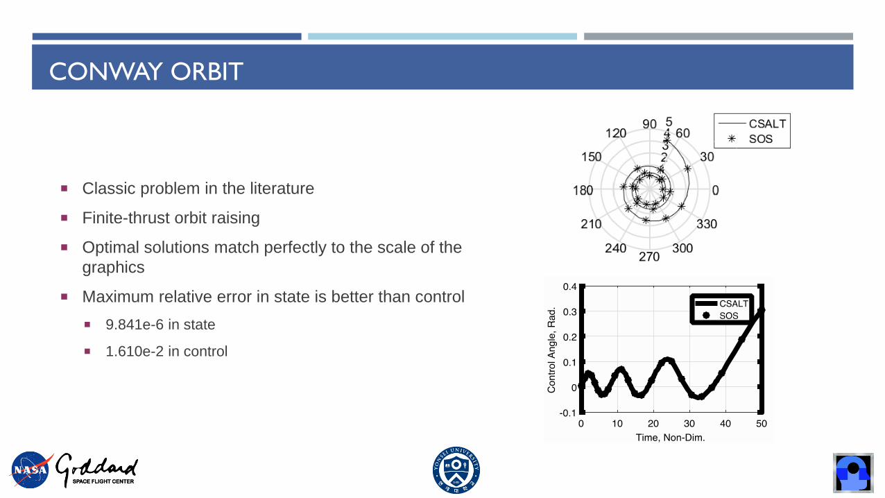
CONWAY ORBIT

Classic problem in the literature

Finite-thrust orbit raising

Optimal solutions match perfectly to the scale of the

graphics

Maximum relative error in state is better than control

9.841e-6 in state

1.610e-2 in control

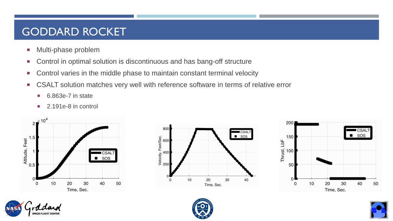
GODDARD ROCKET

Multi-phase problem

Control in optimal solution is discontinuous and has bang-off structure

Control varies in the middle phase to maintain constant terminal velocity

CSALT solution matches very well with reference software in terms of relative error

6.863e-7 in state

2.191e-8 in control

HYPERSENSITIVE PROBLEMTable 2. High level optimal control comparisons


Rayleigh


Rayleigh


straint)

SOS 6.59E-08
















Hull Problem 9.5 2.876e-09 2.817e-08


0 0.5 1 1.5 2

Time, non-dim.

0

1

2

Sta

te,

no

n-d

im.

CSALT

Exact

0 0.5 1 1.5 2

Time, non-dim.

0

0.5

1

Co

ntr

ol, n

on

-dim

.

CSALT

Exact



















0 5 10 15 20 25

Time, Non-Dim.

0

0.5

1

Sta

te,

No

n-D

im.

CSALT

GPOPSII


0 10 20 30

Time, Non-Dim.

-0.4

-0.3

-0.2

-0.1

0

Co

ntr

ol N

on

-Dim

.

CSALT

GPOPSII











1.610e-02.













Goddard SOS 6.863e-07 2.191e-08


Conway SOS 9.814e-06 1.610e-02

4

Stressing case to the mesh refinement algorithm

Dynamics rapidly change near the boundary conditions,

but are nearly constant in between

Relative errors are larger than desirable

4.305e-2 in state

2.911e-1 in control

Believed to be due to interpolation to common discretization

times (and away from the collocation points)

This is supported by the relative error between SOS and

GPOPS-II (3.54e-1 and 1.037 in state and control

respectively)

AGENDA

Motivation


CSALT



Summary/Future Work

MARS TRANSFERTable 5. Earth to Mars solutions comparison

Parameter Malto HILTOP CSALT

Launch date 3/29/2022 4/7/2022 4/4/2022

Launch C3 (km2/s2) 32.26 32.57 35.06

Launch declination (deg) -5.1 -3.776 -5.067

Launch mass (kg) 2,105.4 2,187.3 2,143.0

Cruise flight time (days) 458.2 455.7 452.0

Cruise propellant (kg) 324.3 338.7 336.9

Mars Arrival date 7/1/2023 7/6/2023 7/1/2023

Table 6. Dawn mission solutions comparison


Leg 1 Earth-Mars

Launch date 9/27/2007 9/27/2007 9/27/2007

Launch C3 (km2/s2) 5.1529 5.2285 1.4819

Launch declination (deg) 28.5 28.5 11.7803

Launch mass (kg) 1,114.4 1,105.2 1243.0

Flight time (days) 510 510 527

Arrival mass (kg) 1,039.8 1,032.7 1180.2

Propellant used (kg) 74.6 72.4 62.8

Leg 2 Mars-Vesta

Swingby date 2/18/2009 2/18/2009 3/7/2009

Swingby v∞ (km/s) 4.10 4.11 4.49

Passage altitude (km) 300 300 300

Flight time (days) 894 827.7 903.1

Arrival date 8/1/2011 5/26/2011 8/27/2011

Arrival mass (kg) 907.3 901.4 1,079.0


Stay time (days) 270 336.3 270

Leg 3 Vesta-Ceres

Departure date 4/27/2012 4/27/2012 5/23/2012

Flight time (days) 1,038 1,038 1,230

Arrival date 2/28/2015 2/28/2015 10/4/2015

Arrival mass (kg) 807.2 802.3 960.1


Total Propellant (kg) 307.2 302.8 282.9

Mission duration (days) 2,711 2,711 2,930

optimization of the Dawn spacecraft’s trajectory. Recall that the

Dawn spacecraft launched on September 27th of 2007, com-

pleted a Mars flyby and rendezvous with Vesta, before a final

rendezvous with Ceres. Again, the full problem set-up is not

repeated here, and can be found in Ref. 12).

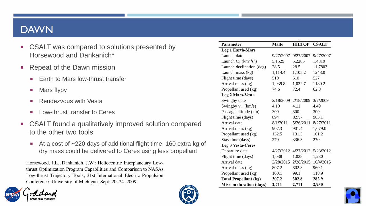
Table 6 compares the trajectories found in the same three op-

timal control solvers. In this case, CSALT found a qualitatively

different trajectory. Whereas, both Malto and HILTOP deter-

mined that a higher energy (C3 < 5 km2/s2) launch at the max-

imum allowable declination was optimal, CSALT proscribes a

much lower energy launch to a relatively low declination. De-

spite the lower launch energy, the CSALT trajectory arrives at

Mars using less propellant, at the cost of only 17 days extra

flight time. Once again, in the second leg of the journey, CSALT

found a control history capable of using roughly 30 kg less pro-

pellant in reaching a rendezvous with Vesta. The flight time was

comparable to the Malto solution, but longer than the HILTOP

solution. The final leg of the flight was somewhat different, as

the CSALT trajectory required a greater amount of propellant

to reach Ceres, in addition to an appreciably longer flight time.

However, the increased propellant on this final leg was not suffi-

Table 7. IRK Solution Comparisons

Rao Automatica Conway Orbit Interior Point

Trap. -6.3978783E-3 9.3879865E-2 9.2193588E-1

HS -8.9985093E-3 9.5179464E-2 9.2053151E-1

RK4 -8.9985093E-3 9.5179464E-2 9.2053151E-1

RK6 -8.9636726E-3 9.5127025E-2 9.2053144E-1

RK8 -8.9637968E-3 9.5123433E-2 9.2053144E-1

Truth -8.9637970E-3 9.5123383E-2 9.2053140E-1

Table 8. IRK Solution Comparisons Using Different Mesh Configurations

Solution Rao Conway Interior Point

Coarse -6.3978783E-3 9.3879865E-2 9.2193588E-1

Fine -8.9621440E-3 9.5132015E-2 9.2056672E-1

Truth -8.9637970E-3 9.5123383E-2 9.2053140E-1

cient to compensate for savings elsewhere, and CSALT found a

solution that would deliver almost 160 kg greater mass to Ceres,

using at least 20 kg less propellant, at a cost of slightly less than

220 days of additional mission duration.

4.5. Selected IRK Problems

In this section we present high level comparison results for

the implicit Runge-Kutta (IRK) methods in CSALT. The meth-

ods implemented are Trapezoid, Hermite-Simpson, and Runge-

Kutta 4/6/8-th order algorithms all of type Lobatto IIIa. Table 7

presents the CSALT solutions for the Rao Automatica, Conway

Orbit Example, and Interior Point problems obtained without

mesh-refinement. Mesh-refinement for IRK methods is under-

way but is not complete at the time of writing. The truth data

for the problems illustrated here is contained in Table 2.

In the absence of mesh-refinement, the quality of the solu-

tion is heavily affected by both the user-defined mesh points

and the order of the collocation method. We expect that when

employing the same mesh configuration, higher order methods

will provide more accurate solutions than lower order methods

and that is confirmed by the data in Table 7. CSALT solutions

converge to the truth data as the order of the method increases

when employing the same mesh. Note, the Hermite-Simpson

method is a fourth order method similar to the Runge-Kutta 4th

order method. Consequently, the results from Hermite-Simpson

and the Runge-Kutta 4th order methods are effectively the same.

Table 8 contains test results for the trapezoidal method for

Rao Automatica, Conway Orbit, and the Interior Point prob-

lems with the original mesh configuration, and a more dense

mesh configuration expected to improve solution quality (effec-

tively by-hand mesh refinement). The original solutions for Rao

Automatica, Conway Orbit, and Interior Point use six, twenty,

and ten, mesh points respectively. The improved solutions for

Rao Automatica, Conway Orbit, and Interior Point use two hun-

dred, two hundred, and sixty, mesh points respectively.

5. Future Work

To date, CSALT development needs were prioritized based

on the needs of low thrust interplanetary missions. Future work

will address other capabilities required for solving more general

optimal control problems, including static and integral decision

parameters and integral constraints. We also plan to implement

second derivatives and interfaces to NLP solvers that support

6

CSALT was compared to solutions presented by

Horsewood and Dankanich*

Direct transfer from Earth to Mars using 2 ion engines

Qualitatively indentical solutions were found using all 3

software tools

The final solutions all match to the expected margin of

error of the modeling techniques

*

DAWN

Table 5. Earth to Mars solutions comparison


Launch date 3/29/2022 4/7/2022 4/4/2022

Launch C3 (km2/s2) 32.26 32.57 35.06

Launch declination (deg) -5.1 -3.776 -5.067

Launch mass (kg) 2,105.4 2,187.3 2,143.0

Cruise flight time (days) 458.2 455.7 452.0

Cruise propellant (kg) 324.3 338.7 336.9

Mars Arrival date 7/1/2023 7/6/2023 7/1/2023

Table 6. Dawn mission solutions comparison


Leg 1 Earth-Mars

Launch date 9/27/2007 9/27/2007 9/27/2007

Launch C3 (km2/s2) 5.1529 5.2285 1.4819

Launch declination (deg) 28.5 28.5 11.7803

Launch mass (kg) 1,114.4 1,105.2 1243.0

Flight time (days) 510 510 527

Arrival mass (kg) 1,039.8 1,032.7 1180.2


Leg 2 Mars-Vesta

Swingby date 2/18/2009 2/18/2009 3/7/2009

Swingby v∞ (km/s) 4.10 4.11 4.49

Passage altitude (km) 300 300 300

Flight time (days) 894 827.7 903.1

Arrival date 8/1/2011 5/26/2011 8/27/2011

Arrival mass (kg) 907.3 901.4 1,079.0


Stay time (days) 270 336.3 270

Leg 3 Vesta-Ceres

Departure date 4/27/2012 4/27/2012 5/23/2012

Flight time (days) 1,038 1,038 1,230

Arrival date 2/28/2015 2/28/2015 10/4/2015

Arrival mass (kg) 807.2 802.3 960.1


Total Propellant (kg) 307.2 302.8 282.9

Mission duration (days) 2,711 2,711 2,930

optimization of the Dawn spacecraft’s trajectory. Recall that the

Dawn spacecraft launched on September 27th of 2007, com-

pleted a Mars flyby and rendezvous with Vesta, before a final

rendezvous with Ceres. Again, the full problem set-up is not

repeated here, and can be found in Ref. 12).

Table 6 compares the trajectories found in the same three op-

timal control solvers. In this case, CSALT found a qualitatively

different trajectory. Whereas, both Malto and HILTOP deter-

mined that a higher energy (C3 < 5 km2/s2) launch at the max-

imum allowable declination was optimal, CSALT proscribes a

much lower energy launch to a relatively low declination. De-

spite the lower launch energy, the CSALT trajectory arrives at

Mars using less propellant, at the cost of only 17 days extra

flight time. Once again, in the second leg of the journey, CSALT

found a control history capable of using roughly 30 kg less pro-

pellant in reaching a rendezvous with Vesta. The flight time was

comparable to the Malto solution, but longer than the HILTOP

solution. The final leg of the flight was somewhat different, as

the CSALT trajectory required a greater amount of propellant

to reach Ceres, in addition to an appreciably longer flight time.

However, the increased propellant on this final leg was not suffi-

Table 7. IRK Solution Comparisons

Rao Automatica Conway Orbit Interior Point

Trap. -6.3978783E-3 9.3879865E-2 9.2193588E-1

HS -8.9985093E-3 9.5179464E-2 9.2053151E-1

RK4 -8.9985093E-3 9.5179464E-2 9.2053151E-1

RK6 -8.9636726E-3 9.5127025E-2 9.2053144E-1

RK8 -8.9637968E-3 9.5123433E-2 9.2053144E-1

Truth -8.9637970E-3 9.5123383E-2 9.2053140E-1

Table 8. IRK Solution Comparisons Using Different Mesh Configurations

Solution Rao Conway Interior Point

Coarse -6.3978783E-3 9.3879865E-2 9.2193588E-1

Fine -8.9621440E-3 9.5132015E-2 9.2056672E-1

Truth -8.9637970E-3 9.5123383E-2 9.2053140E-1

cient to compensate for savings elsewhere, and CSALT found a

solution that would deliver almost 160 kg greater mass to Ceres,

using at least 20 kg less propellant, at a cost of slightly less than

220 days of additional mission duration.

4.5. Selected IRK Problems

In this section we present high level comparison results for

the implicit Runge-Kutta (IRK) methods in CSALT. The meth-

ods implemented are Trapezoid, Hermite-Simpson, and Runge-

Kutta 4/6/8-th order algorithms all of type Lobatto IIIa. Table 7

presents the CSALT solutions for the Rao Automatica, Conway

Orbit Example, and Interior Point problems obtained without

mesh-refinement. Mesh-refinement for IRK methods is under-

way but is not complete at the time of writing. The truth data

for the problems illustrated here is contained in Table 2.

In the absence of mesh-refinement, the quality of the solu-

tion is heavily affected by both the user-defined mesh points

and the order of the collocation method. We expect that when

employing the same mesh configuration, higher order methods

will provide more accurate solutions than lower order methods

and that is confirmed by the data in Table 7. CSALT solutions

converge to the truth data as the order of the method increases

when employing the same mesh. Note, the Hermite-Simpson

method is a fourth order method similar to the Runge-Kutta 4th

order method. Consequently, the results from Hermite-Simpson

and the Runge-Kutta 4th order methods are effectively the same.

Table 8 contains test results for the trapezoidal method for

Rao Automatica, Conway Orbit, and the Interior Point prob-

lems with the original mesh configuration, and a more dense

mesh configuration expected to improve solution quality (effec-

tively by-hand mesh refinement). The original solutions for Rao

Automatica, Conway Orbit, and Interior Point use six, twenty,

and ten, mesh points respectively. The improved solutions for

Rao Automatica, Conway Orbit, and Interior Point use two hun-

dred, two hundred, and sixty, mesh points respectively.

5. Future Work

To date, CSALT development needs were prioritized based

on the needs of low thrust interplanetary missions. Future work

will address other capabilities required for solving more general

optimal control problems, including static and integral decision

parameters and integral constraints. We also plan to implement

second derivatives and interfaces to NLP solvers that support

6

CSALT was compared to solutions presented by

Horsewood and Dankanich*

Repeat of the Dawn mission

Earth to Mars low-thrust transfer

Mars flyby

Rendezvous with Vesta

Low-thrust transfer to Ceres

CSALT found a qualitatively improved solution compared

to the other two tools

At a cost of ~220 days of additional flight time, 160 extra kg of

dry mass could be delivered to Ceres using less propellant

AGENDA

Motivation


CSALT



Summary/Future Work

SUMMARY AND FUTURE WORK

CSALT is a mature software package capable of solving a variety of optimization problems with high

accuracy

CSALT has been successfully benchmarked against industry standard tools in both general engineering

problems and for the solution of low-thrust trajectories

Future Work

Static and integral decision parameters and integral constraints

Second derivatives of the collocation

Improve performance

Full integration into GMAT

benchmarking the collocation stand- alone library … · benchmarking the collocation stand-alone...

Documents