bending - ddd.uab.cat · pdf filebehavior study of pipes after forming, coating and bending...
TRANSCRIPT

Behavior Study of Pipes after Forming, Coating and Bending
Page 1 of 85
The down sign NOTIFY that the present project with the title:
Behavior Study of Pipes after Forming, Coating and Bending and determined for Jordi Marquez Llinás by eligibility for the qualification of the Degree in Materials
Engineering in Universitat Autònoma de Barcelona, has been made under the university management being all
the results and procedures in the present documentation done for the above mentioned.
For this purpose, the present certificate is signed by:
PHd. Baró M.D Head of Materials Physics II Department
Universitat Autònoma de Barcelona

Behavior Study of Pipes after Forming, Coating and Bending
Page 2 of 85
Acknowledgements
It is my sincerely wish to dedicate this project without any order of importance to:
My parents and part of the family, especially my cousin Ramon and Ana for all the truly and unconditional
love and support to my person in the good and not so good moments.
Moi my childhood friend for all these years by my side offering me always the best of himself.
Núria to change much of my life and for all the love and understanding towards me.
Edu for the unconditional and sincerely help and support both in Spain and Belgium and all the good
moments lived always.
Cristiane for returning to the faith in many things and offer me the best of yourself sincerely and
selflessly.
Dolors Baró, to trust in me allowing and opening this quite desired way to do this project abroad.
OCAS for giving me the opportunity of these 6 months of internship.
CFGS my Sabadell teachers, especially Santandreu and Rafa, infusing me new hopes for returning to finish
my studies and career.
Tania and Carlos for their support and patience in some really bad moments.
Marga and Pau for your sincerity and all the entire conversations and great moments shared.
And in memory of my aunt, Luisa, who taught me so much offering the best of herself without asking
anything in return, with her best smile, happiness and energy.
Gratefully thanks to all of you with my whole heart.

Behavior Study of Pipes after Forming, Coating and Bending
Page 3 of 85
Table of Contents
1 INTRODUCTION ............................................................................................................................................... 5
1.1 HISTORY OF PIPELINES ............................................................................................................................. 5
1.2 PIPELINES LOCATIONS AND ENVIRONMENTS .......................................................................................... 6
1.3 PROCEDURES OF PIPELINES MANUFACTURING ...................................................................................... 7
1.3.1 SEAMLESS ........................................................................................................................................ 7
1.3.2 LONGITUDINALLY WELDING USING ELECTRICAL RESISTANCE WELDING (ERW) ............................. 8
1.3.3 LONGITUDINALLY WELDING USING SUBMERGED ARC WELDING (SAW) ........................................ 9
1.3.4 HELICAL OR SPIRAL WELDED ......................................................................................................... 11
1.4 PIPELINES STEELS ................................................................................................................................... 11
1.5 PIPELINES COATINGS ............................................................................................................................. 15
2 JUSTIFICATION AND OBJECTIVES ................................................................................................................... 16
3 EXPERIMENTAL METHODOLOGY ................................................................................................................... 17
3.1 SAMPLING AND COATING RECREATION ................................................................................................ 17
3.2 TENSILE TEST .......................................................................................................................................... 18
3.2.1 MECHANICAL PROPERTIES ............................................................................................................ 19
3.2.2 EXPERIMENTAL TENSILE TEST DESCRIPTION ................................................................................. 23
3.3 HEAT TRANSFERS IN CHARPY V‐NOTCH ................................................................................................ 24
3.3.1 ENERGY TRANSFER ........................................................................................................................ 24
3.3.2 ANALYTICAL DESCRIPTION ............................................................................................................. 27
3.3.3 EXPERIMENTAL HEAT TRANSFER CHARPY V‐NOTCH PROCEDURE ................................................ 33
3.4 CHARPY V‐NOTCH IMPACT TEST ............................................................................................................ 35
3.4.1 CHARPY TEST METHOD .................................................................................................................. 36
3.4.2 MECHANICAL FRACTURES AND DBTT IN CHARPY ......................................................................... 37
3.4.3 EXPERIMENTAL CHARPY V‐NOTCH PROCEDURE ........................................................................... 39

Behavior Study of Pipes after Forming, Coating and Bending
Page 4 of 85
3.5 FEM SIMULATION .................................................................................................................................. 41
3.5.1 GENERAL SIMULATION STRUCTURE STUDY CASE ......................................................................... 41
3.5.2 PREPROCESSING AND MODEL SET‐UP........................................................................................... 47
4 RESULTS AND DISCUSSION ............................................................................................................................ 60
4.1 SAMPLING AND COATING RECREATION ................................................................................................ 60
4.2 TENSILE TEST .......................................................................................................................................... 61
4.3 HEAT TRANSFERS IN CHARPY V_NOTCH TEST ....................................................................................... 66
4.3.1 ANALYTICAL PROCEDURE .............................................................................................................. 66
4.3.2 EXPERIMENTAL PROCEDURE ......................................................................................................... 72
4.4 CHARPY V‐NOTCH IMPACT TEST ............................................................................................................ 74
4.5 FEM SIMULATION .................................................................................................................................. 77
5 CONCLUSIONS ............................................................................................................................................... 81
6 FUTURE WORKS ............................................................................................................................................. 82
7 ENVIRONMENTAL ASPECTS ........................................................................................................................... 82
8 COSTS ............................................................................................................................................................. 83
9 REFERENCES................................................................................................................................................... 85

Behavior Study of Pipes after Forming, Coating and Bending
Page 5 of 85
1 INTRODUCTION
1.1 HISTORY OF PIPELINES
The first pipeline was built in the United States in 1859 for the transport of the crude oil [1]. Through the one‐
and‐a‐half century of pipeline operating services, the petroleum industry, which has been acquiring each year
more importance, has proven that pipelines are by far the most economical means of large scale overland
transportation for crude oil, natural gas, and their products versus rail, ship and truck transportation.
According to the industrialization age, these types of products to obtain energy are demanded in more large
quantities to be moved on a regular basis, being this differences more clear every year.
Due to the transport of petroleum fluids with pipelines is a continuous and reliable operation, and the ability
to adapt to a wide variety of environments such remotes areas, hostile environments, etc. the use of pipelines
have been increased and nowadays, are used to connect countries and continents with the areas where is
extracted and the refineries so offshore pipelines can be classified as follows (Figure 1.1):
Fig.1.1 – Offshore subsea pipeline use
• Flowlines transporting oil and/or gas from satellite subsea Wells to subsea manifolds.
• Flowlines transporting oil and/or gas from subsea manifolds to production facility platforms.
• Infield Flowlines transporting oil and/or gas between production facility platforms to shore.
• Flowlines transporting water or chemicals from production facility platforms through subsea injection
manifolds to injection wellheads.
• Flowlines transporting oil and/or gas from shore to refineries to be treated and distributed.

Behavior Study of Pipes after Forming, Coating and Bending
Page 6 of 85
1.2 PIPELINES LOCATIONS AND ENVIRONMENTS
Nowadays, exist a global worldwide wire of pipelines for the crude distribution around the world, in fact,
usually the oil fields are placed so far from the consumption areas. In example, Occidental Europe exports 97%
of its necessities mainly from Africa or Western Asia (Figure 1.2). Other countries such Russia, EEUU, Canada,
etc., also need to export crude oil from very far regions.
Fig. 1.2 – European and Western Asia crude oil and gas pipelines connection
Each earth region, has specific environmental conditions and also quite different geography conditions, from
the crude source to final destination so the needed locations of the pipelines routes have to be adapted
according the geography and land possibilities as well the most beneficial economical factors. Different
locations are shown below (Figure 1.3 a, b, & c):
Fig. 1.3 – a) Extreme cold environment(Alaska) b)Moderate environment c)Extreme hot environment (Desert of
Arabia)

Behavior Study of Pipes after Forming, Coating and Bending
Page 7 of 85
1.3 PROCEDURES OF PIPELINES MANUFACTURING
Nowadays, for oil and gas industry, the pipes are commonly made by one of following four fabrication
procedures [2]:
1.3.1 SEAMLESS
Seamless pipe is formed by hot working steel to form a pipe without a welded seam. This procedure can be
done by different ways.
The initially formed pipe may be subsequently cold worked to obtain the required diameter and wall thickness
and after heat treated to modify the mechanical properties. To obtain the pipe, a solid steel bar is firstly drilled
from a slab and is subsequently heated and formed by rollers around a piercer to produce the length of the
pipe (Figure 1.4).
Fig. 1.4 – Seamless pipe process
The main disadvantages of this procedure are: higher costs to obtain in comparison with alternative
procedures, although the process is quite slow (rollers usually turning between 100‐150RPM in function of
diameter), other disadvantages are a fairly wide variation of wall thickness (around 15%) and out of roundness
and straightness.

Behavior Study of Pipes after Forming, Coating and Bending
Page 8 of 85
1.3.2 LONGITUDINALLY WELDING USING ELECTRICAL RESISTANCE WELDING (ERW)
ERW pipe is formed from coiled plate steel. The plate is uncoiled and sheared to the required width, flattened
and the edges are dressed. The plate is passed through a sequence of rolls to form the pipe, crimping the
edges of the plate and then progressively bending the plate into a circular final form, ready for welding in the
longitudinal direction (Figure 1.5):
Fig. 1.5 – ERW Process
The welding step, consist on applying electrical current across the interface of the steel pipe needed to be
heated for welding, obtaining a heating in both pipe faces to be welded. Once heated the faces are pressed
together to produce the longitudinal seam weld using induction coils operating at low frequency (60‐360Hz of
AC) or induced into the steel with induction coils operating at high frequencies of above 400KHz, termed High
Frequency Induced (HFI) ERW procedure.
HFI, is commonly used for submarine pipelines due to HAZ (Heat Affected Zone) is slower than the other
methods, because of the electrons that carry the current tend to flow increasingly at the outer surface of the
conductor and at high frequencies the electron movement is exclusively in the outer 1mm or less of the
conductor, allowing to the pipe walls to melt in a very small area long to longitudinal direction.

Behavior Study of Pipes after Forming, Coating and Bending
Page 9 of 85
1.3.3 LONGITUDINALLY WELDING USING SUBMERGED ARC WELDING (SAW)
The pipe is formed from individual plates of steel and subsequently applying 4 steps once the plate is trimmed.
For the forming steps it is also commonly named, U‐O‐E process [3].
• FIRST STEP
First forming step involves crimping of the edges of the plate into circular arcs over a width of about one radius
on each side pressing the ends between two shaped dies applying it in several steps due to the high pressure
that is needed (Figure 1.6):
Fig. 1.6 – First step forming
• SECOND STEP FORMING
On second step forming process the plate moves to U‐press where centered the U‐punch moves down and
bens the entire plate through three‐point bending. The U‐punch is held in place and the side rollers are moved
inwards (Figure 1.7):
Fig. 1.7 – Second forming process

Behavior Study of Pipes after Forming, Coating and Bending
Page 10 of 85
• THIRD FORMING STEP
In the third forming step, the skelp is then conveyed to the O‐press consisting of two semi‐circular stiff dies
(Figure 1.8). The top die is actuated downwards forcing the skelp into a nearly circular shape.
Fig. 1.8 – Third forming process
• FOURTH FORMING STEP
On this step the skelp is welded and a final expansion step is accomplished by an internal mandrel achieving
low ovality due that the pipe is expanded from 0.8 to 1.3% from its diameter after the O‐step (Figure 1.9):
Fig. 1.9 – a) SAW Longitudinal Welding b)Fourth forming Expansion step

Behavior Study of Pipes after Forming, Coating and Bending
Page 11 of 85
1.3.4 HELICAL OR SPIRAL WELDED
For this procedure, a coil of hot‐coiled plate is uncoiled, straightened, flattened and edges dressed. Then the
plate is helical wound to form a pipe which its diameter depends of the width of the strip and the angle of
coiling. Once is formed, the helical internal seam is welded using SAW or inert gas, and as the seam rotates to
the top position, the external weld is made (Figure 1.10), obtaining a continuous length of pipe which is passed
through a sequence of rollers to enhance circularity. Finally the pipe is tested using radiography or ultrasonic
testing and finally cutted to the required lengths.
Fig. 1.10 – Spiral Welded Pipe Process
1.4 PIPELINES STEELS
Pipeline steel must have high strength while retaining ductility, fracture toughness and weldability [1][4].
• Strength is the ability of the pipe steel and the associated welds, to resist longitudinal and transverse
tensile forces imposed on the pipe in service and during installation.
• Ductility is the ability of the pipe to absorb overstressing by deformation.
• Toughness is the ability of the pipe material to withstand impacts or shock loads and the behavior of
the material is very important, indeed, brittle or ductile fracture manner.
• Weldability is the ability and ease of production of a quality weld with an adequate strength and
toughness in the HAZ.
The balance of properties (strength, toughness and weldability) required depends on the intended use of the
pipeline. Due to the increasingly energetic demand in last decades, since mid 1960s, the requirements become
more exigent and also the transport reduction costs. For these reasons more standards (regulated by API,
American Petroleum Institute, ASME, American Society of Mechanical Engineers, ISO, International Standards
Organization, etc…) have been developed to standardize the entire pipelines world.

Behavior Study of Pipes after Forming, Coating and Bending
Page 12 of 85
Due to the higher operating pressures the diameter of the pipes was increased and also in service
requirement. For this purposes thicker wall pipes were needed.
The primary design parameter for this effort is the Yield Strength (YS) because as the YS increases, the wall
thickness requirement decreases. It is needed to take into account also the environmental effects, pipe
manufacturing procedures, the type of fluids and the in service operating conditions.
Engineering materials have four essential characteristics that are closely interrelated:
• Chemistry: The primary element (Fe), alloying elements (Ni, Cr, etc. with ferrous metals), unintended elements and impurities of other elements.
• Physical properties: Density, modulus of elasticity, coefficient of thermal expansion, electrical and heat conduction, etc.
• Microstructure: Atomic structure, metallurgical phases, type and size of grains.
• Mechanical properties: YS (ultimate elongation at rupture), toughness (Charpy nil ductility transition temperature, fracture toughness).
The materials used in pipelines systems can be classified in two large categories: metallic and non‐metallic.
Focusing on metallic exist also two internal categories: ferrous (Fe based) or non‐ferrous (Cu, Ni or Al based).
Nowadays, the most widely steel grades used are x65, x70, x80 and x100. This project is focused only in x65.
Regarding standard API 5L for pipelines, the maximum component amount allowed for x65 pipeline steel
grades are shown following (Table 1.1):
Maximum Chemical % of Weight in X65 Steel Grade welded
CMAX Mn P
SMAX Min Max Min Max
0.30 ‐‐‐‐ 1.8 0.045 0.08 0.03
Tab. 1.1 – Maximum Chemical %Weight for x65 (API 5L)
This standard also fix the minimum YS in (PSI) that corresponds to the number used to define the steel grade,
in this case 65PSI (448MPa).
Behavior Study of Pipes after Forming, Coating and Bending
Page 13 of 85
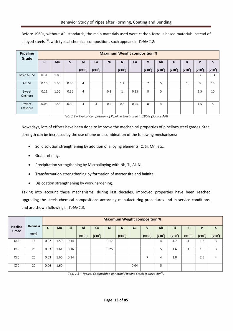
Before 1960s, without API standards, the main materials used were carbon‐ferrous based materials instead of
alloyed steels [5], with typical chemical compositions such appears in Table 1.2:
Pipeline Grade
Maximum Weight composition %
C Mn Si Al
(x102)
Ca
(x103)
Ni N
(x102)
Cu V
(x102)
Nb
(x102)
Ti
(x102)
B
(x103)
P
(x102)
S
(x102)
Basic API 5L 0.31 1.80 3 0.3
API 5L 0.16 1.56 0.35 4 1.2 7 5 1 3 15
Sweet Onshore
0.11 1.56 0.35 4 0.2 1 0.25 8 5 2.5 10
Sweet Offshore
0.08 1.56 0.30 4 3 0.2 0.8 0.25 8 4 1.5 5
Tab. 1.2 – Typical Composition of Pipeline Steels used in 1960s (Source API)
Nowadays, lots of efforts have been done to improve the mechanical properties of pipelines steel grades. Steel
strength can be increased by the use of one or a combination of the following mechanisms:
• Solid solution strengthening by addition of alloying elements: C, Si, Mn, etc.
• Grain refining.
• Precipitation strengthening by Microalloying with Nb, Ti, Al, Ni.
• Transformation strengthening by formation of martensite and bainite.
• Dislocation strengthening by work hardening.
Taking into account these mechanisms, during last decades, improved properties have been reached
upgrading the steels chemical compositions according manufacturing procedures and in service conditions,
and are shown following in Table 1.3:
Pipeline Grade
Thickness
(mm)
Maximum Weight composition %
C Mn Si Al
(x102)
Ca
(x103)
Ni N
(x102)
Cu V
(x102)
Nb
(x102)
Ti
(x102)
B
(x103)
P
(x102)
S
(x102)
X65 16 0.02 1.59 0.14 0.17 4 1.7 1 1.8 3
X65 25 0.03 1.61 0.16 0.25 5 1.6 1 1.6 3
X70 20 0.03 1.66 0.14 7 4 1.8 2.5 4
X70 20 0.06 1.60 0.04 5
Tab. 1.3 – Typical Composition of Actual Pipeline Steels (Source API[6])

Behavior Study of Pipes after Forming, Coating and Bending
Page 14 of 85
The chemical compositional changes from 60s until now are due to the role of each element in the material
properties, the most important are:
• C – Increases strength (yield and ultimate) and also hardness, but reduces ductility (elongation and rupture) and notch toughness (using high amounts, Charpy tests exhibits nil brittle‐ductile transition temperature, BDTT). It also affects weldability, being more difficult to control in the process.
• Mn – Deoxidizes and desulfurizes steel avoiding brittle iron‐sulfides, refining the grain and improving hot‐workability. It is demonstrated that if ratio Mn/C>3 the Mn improves impact toughness and above 0.8% Mn tends to harden steel.
• Si – Improves castability because of is a deoxidizer that captures dissolved oxygen avoiding porosities.
• Ni – Causes a significant improvement in fracture toughness and fatigue resistance.
• Cu – Improve atmospheric corrosion resistance.
• V – Refines steel grains, improving its mechanical properties and its resistance to H attack.
• S – Is contained in the steel and is considered as an impurity that forms brittle crack‐prone iron sulfide.
• P – Increases ultimate strength (US) of the steel. Otherwise is considered an impurity because forms brittle, crack‐prone iron‐phospite during heat‐treatments or at high temperature services.

Behavior Study of Pipes after Forming, Coating and Bending
Page 15 of 85
1.5 PIPELINES COATINGS
Pipelines need to be protected under corrosion effects [1][7](CD DOCUMENTATION/COATINGS). The main
purpose of coating is to isolate the pipe steel from the environment: soil, seawater, rain, etc. and to present a
high resistance path between anodic and cathodic areas. Table 1.4, summarizes the different steps with its
range of temperatures to apply on coatings processes:
NAME PIPE TEMPERATURE (ºC) TIME (s) OBSERVATIONS
SURF
ACE
Water washing Hot water or steam ‐‐ ‐‐
Dry and Preheating In function of subsequently coating ‐‐ ‐‐
Blast cleaning ‐‐ ‐‐ Can affect to mechanical properties
Coating adhesion 120 At least 20
Chemical pretreatment (phosphoric acid) and chromate conversion coating
COATING
Asphalt Enamel 250 *1(maximum) Inner preheat at 40ºC ‐‐ After coating, quenched. Ts= 65‐75ºC
FBE[8] 220 ‐‐ Electrostatically heated; Ts=70ºC
PE/PU/PP 220 ‐‐ Electrostatically heated and water quenched at 80ºC. PE Ts=85ºC; PU Ts=100ºC; PP Ts=75‐140ºC
Elastomeric Coating (Neoprene) 145 2 (hours)
P=500 KPa (vulcanization)
Thermal Insulation 220 ‐‐ Electrostatically heated
Ts : Temperature in service; P : Pressure; NOTE: Pipe temperature is the temperature of the pipe when the coating is applied. *1 is the maximum reachable temperature of the coating
product and not the steel temperature. Tab. 1.4 – Pipe surface preparation and coatings summary
As can be observed in Table 1.4 a previous surface treatment is required for the assurance a good steel surface
and to avoid defects on the coating process. Dry and pre‐heat stage, is function of the subsequent coating
process.
Blast cleaning can affect the mechanical properties of the steel being similar than a micro shoot‐penning
process, indeed, higher pre‐strain value can be induced, Figure 1.11 , although the heat applied during the
coating steps can help to recover partially its initial values.
Fig. 1.11– Blast cleaning process
The maximum temperature reached by the pipe steel is 220ºC by electrostatically heating. In the case of
Asphalt Enamel maximum temperature of 250ºC can be reached by the coating product directly applied to the
pipe steel.

Behavior Study of Pipes after Forming, Coating and Bending
Page 16 of 85
2 JUSTIFICATION AND OBJECTIVES
Arcelor Mittal delivers hot rolled products from coil for the energy market, which are subsequently formed
and welded to produce pipelines for oil and gas transportation. The guaranteed mechanical properties such as
yield stress, tensile strength, toughness, elongation, tend to decrease due the forming procedures from coil to
pipe. These mechanical properties can be predicted using numerical models capable of describing its evolution
during pipe manufacturing. Nonetheless, this guarantee cannot take into account the evolution of the pipe
properties during downstream processing. Indeed, once the pipe is sold, it needs to be coated, installed,
welded and sometimes bent.
The objective of the project is obtain a better understanding of the influence of the coating, which is a thermal
cycle, straining and in field‐bending in the mechanical properties of the material.
For this purpose, a study of coating methods has been done, in order to define the industrial pipe thermal
cycles. Experimental tests are also carried out to provide a better understanding of the influence of the
thermal cycles on the base material once is prestrained due the UOE pipe forming process.
Experimental tests consist on tensile test, to obtain the mechanical properties in both conditions: as received
material, it means without coating, and once the material is coated. Energetic test, Charpy V‐Notch (CVN)
impact test is also necessary for a better understanding of the capability of the material to absorb impact
energy and for the determination of the Brittle‐Ductile Transition Temperature (BDTT) of the coated material.
CVN impact tests are usually done in a very low range of temperatures. Due that the samples are handled from
the freezer to the test machine until hammer impacts on it, only the initial temperature is well known. To
know the final CVN sample temperature once the hammer impact an analytical heat transfer model have been
developed and validated to predict the temperature. It also means the increase in order to assure the
experimental quality on this test.
A Finite Element Model (FEM) simulation is carried out to simulate a general cold bending process to predict
the final mechanical properties of x65 steel grade under a cold bending process.

Behavior Study of Pipes after Forming, Coating and Bending
Page 17 of 85
3 EXPERIMENTAL METHODOLOGY
3.1 SAMPLING AND COATING RECREATION
To perform the tests all the samples have been heat treated to recreate using a conventional industrial furnace
similar heat conditions that are applied in a real coating industrial pipes processes.
The specimens are taken out in transversal direction, opposite side of the weld, being a base not welded
material (Figure 3.12), and finally machined by milling.
Fig. 3.12 – Samples area base material location
According coating processes, two different temperatures (minimum and maximum) and two different times of
application (quickly and slower coating process) have been selected, as can be seen in the following Table 3.1:
Heat treatment ID Time [s] Temperature [ºC] T1 30±2 140±1 T2 300±2 140±1 T3 30±2 245±1 T4 300±2 245±1
Table 3.1: Sample identification
The samples have been introduced inside the industrial furnace, and heated up to selected temperature. At
the same time a dummy sample of X65 according standard ISO148‐1 for the Charpy sample dimension
equipped with a type K thermocouple have been connected to a computer to control the real temperature of
the samples and register it. Notice that the tensile samples, have been treated together with the Charpy
samples.

Behavior Study of Pipes after Forming, Coating and Bending
Page 18 of 85
3.2 TENSILE TEST
The experimental tests that can be applied to the materials to know their properties can be [9]:
• Physical Tests. Hardness, Stress, Impact toughness, Fatigue, Heat transfer, etc.
• Chemical Tests. To know qualitative and quantitative composition, corrosion, etc.
• Physical‐Chemical Tests. Macro and microscopically tests with chemical attacks and subsequently
physical tests, etc.
• Electrical Tests. Magnetism behaviour, Dielectric breakdown voltage, etc.
Also experimental tests can be categorized in: Destructive or Non‐ Destructive Tests.
The tensile test is a destructive physical test and is typical used to determine the basic physical properties of
the materials that constitute the basic principles of deformation and fracture.
In general, tensile tests are performed on cylindrical specimens (see Figure 3.16) or parallel‐piped specimens
(sheet and plate). The samples are loaded uniaxially along the length of the specimen being the applied load
and extension (change in length) of the sample simultaneously measured [10].
The recorded strain and stress depict a typical curve such is following (Figure 3.13):
Fig. 3.13 – Typical Engineering Strain‐Stress curve
In the elastic and uniform plastic flow areas, the deformation in the sample is homogenously in the whole
cross section despite in Non Uniform plastic flow Area the deformation appears focused in the central section
of the sample due the material striction exhibiting the classical neck form (according to Schmidt’s Law), where
the sample broke.

Behavior Study of Pipes after Forming, Coating and Bending
Page 19 of 85
3.2.1 MECHANICAL PROPERTIES
The main mechanical properties to obtain from tensile test are:
3.2.1.1 ENGINEERING STRESS AND ENGINEERING STRAIN
Engineering stress is defined like the quotient between the applied uniaxial force and the initial sample
cross section:
(Eq. 1)
Where:
• P : Applied force [N] • Ao : Initial Sample Cross Section [m2]
• σ N K Pa
Engineering strain ( ) is defined like the quotient between length increment (change of length) and the initial
length:
∆
(Eq. 2)
Where:
• lo : Initial length of the sample • lf : Final length of the sample
This analysis facilitates the comparison of results obtained when testing samples that differ in thickness or
geometry.
3.2.1.2 TRUE STRESS ANS TRUE STRAIN
Although engineering values are adequate, the best measures of the response of a material to loading are the
true stress (σ) and true strain (ε) determined, in this case, by the instantaneous dimensions of the tensile
specimen due to the changes while the force is applied. It consists in the increase of the length in the axial
direction with a parallel decrease, however and in the same time, in the cross section.
Because the instantaneous dimensions of the specimen are not typically measured, the true stress and true
strain may be estimated using the engineering stress and engineering strain. It is noted that these estimations
are only valid during uniform elongation and are not applicable throughout the entire deformation range.

Behavior Study of Pipes after Forming, Coating and Bending
Page 20 of 85
True strain is defined like the quotient between the changes in the length and the instant length:
So:
ln ln 1
(Eq. 3)
And assuming that the sample has not any change in its volume, using equation 3, true stress can be defined as
follows:
1
(Eq. 4)
3.2.1.3 TENSILE STRENGTH
The tensile strength is a term which refers to the amount of tensile stress that a material can withstand just
before the effective fracture or failure. It is equivalent to the maximum load (PMAX) that can be carried by one
square millimeter of cross‐sectional area when the load is applied as uniaxial stress, and can be defined using
the following expression:
(Eq. 5)
3.2.1.4 YIELD STRENGTH
In the initial stages of deformation, generally stress changes linearly with the strain. In this region, all
deformation is considered to be elastic because the sample will return to its original shape (initial dimensions)
when the applied stress is removed. If, however, the sample is not unloaded and deformation continues, the
stress‐versus strain curve becomes nonlinear causing a permanent elongation named plasticity.
The stress at which a permanent deformation occurs is called the elastic (or proportional) limit; however,
offset yield strength (0.2% and 0.5% of offset) are typically used to quantify the onset of plastic deformation
due to the ease and standardization of measurement.

Behavior Study of Pipes after Forming, Coating and Bending
Page 21 of 85
3.2.1.5 DUCTILITY
Ductility is the ability of a material to deform plastically without fracturing. The test sample elongates during
the tension test and correspondingly reduces its cross‐sectional area. These two measures of the ductility of a
material are the amount of elongation and reduction in area that occurs during the tension test and can be
expressed like the following equation:
% 100
(Eq. 6)
3.2.1.6 STRAIN‐HARDENING EXPONENT
The flow curve of many metals in the region of uniform plastic deformation can be expressed by the following
simple power curve expression:
(Eq. 7)
Where:
• n : Strain‐hardening exponent • K: Strength coefficient to reach ε=1.
3.2.1.7 RESILIENCE [11]
Resilience is the property of a material to absorb energy when it is deformed elastically recovering it once
unloading. In other words, it is the maximum energy per unit volume elastically stored. It is represented by the
area under the curve in the elastic region in the Stress‐Strain diagram (Figure 3.14) and can be expressed as
follows:
Fig. 3.14 – Typical Engineering Strain‐Stress curve

Behavior Study of Pipes after Forming, Coating and Bending
Page 22 of 85
3.2.1.8 TOUGHNESS
The toughness of a material is its ability to absorb energy in the plastic range [12]. Toughness may be
considered to be the total area under the stress‐strain curve (Figure 3.15) which is referred to as the modulus
of toughness (UT) is an indication of the amount of work per unit volume that can be done on the material
without causing it to rupture.
Fig. 3.15 – Typical Engineering Strain‐Stress curve
As can be observed in the Figure 3.15 two different main groups of toughness are showed referenced with the
most important types of fractures (see Chapter 3.4.2), brittle and ductile fracture. The ductile fracture (green
curve) corresponds with the higher area indicating that more amount of energy can be absorbed for the
material before fracture. It is due the high plasticity of the material.
The orange curve corresponds with the opposite case, the brittle fracture with quite less area showing clearly
that lower plasticity is supported.
The ability to withstand occasional stresses above the yield stress without fracturing is particularly desirable in pipelines (ductile fracture behavior).

Behavior Study of Pipes after Forming, Coating and Bending
Page 23 of 85
3.2.2 EXPERIMENTAL TENSILE TEST DESCRIPTION
All tensile tests are performed on an electro‐mechanical testing machine Zwick Z250.
During the tensile test 2 crosshead speeds are used, namely:
• First traverse speed: position controlled 20MPa/s from: start until Rp0.2.
• Second traverse speed: position controlled 0.00025/s from Rp0.2 until fracture.
Each tensile test is made for each heat treatment and for it, 3 different specimens have been tested,
identifying (ID) each specimen.
The sample description is given in Table 3.2:
Sample ID Description Material Base‐x Base material Material x65 Pipe #3 After PWHT
Diameter 24", Wall thickness 14.8 mm
Pipe ID H473/6‐52 5/11 Coil 1737040
T1‐x Simulation 1 T2‐x Simulation 2 T3‐x Simulation 3 T4‐x Simulation 4
x: repetition 1 to 3 Table 3.2: Sample identification
The tensile tests are performed on round API specimens (Figure 3.16), according to standard ASTM A370, with
a nominal diameter of 6.300±0.005 mm, Lc = 30.000±0.010 mm and reference length Lo = 25.000±0.050 mm.
Fig. 3.16 – Tensile test ASTM A370 sample

Behavior Study of Pipes after Forming, Coating and Bending
Page 24 of 85
3.3 HEAT TRANSFERS IN CHARPY V‐NOTCH
Charpy Impact tests are very common and usefully to obtain information of the materials subjected to
dynamic loads [13][14] (see Chapter 3.4) being very interesting to know the value of the temperature in the
sample during the whole test. To solve this issue, is necessary previous basic knowledge of thermodynamics.
Two bodies at different temperature tend to compensate it, until the same temperature is reached for both[15].
This is accomplished by the transfer of energy from the warm medium to the cold one so the energy transfer is
always from the higher temperature medium to the lower temperature one. The temperature difference is the
driving force for heat transfer.
The rate of heat transfer in a direction depends on the magnitude of the temperature gradient (the
temperature difference per unit length, ΔT) in that direction. The larger ΔT, the higher the rate of heat transfer.
Energy can exist in numerous forms, such as thermal, kinetic, potential, etc. and their sum constitutes the total
energy (E) of a system. The forms of energy related to the molecular structure of a system and the degree of
the molecular activity are referred to as the microscopic energy. The sum of all microscopic forms of energy is
called the internal energy of a system, U [J].
The internal energy may be viewed as the sum of the kinetic and potential energies of the molecules. The
average velocity and the degree of activity of the molecules are proportional to the temperature. Thus, at
higher temperatures the molecules will possess higher kinetic energy, and as a result, the system will have a
higher internal energy. This internal energy is also associated with the intermolecular forces between the
molecules of a system, forces that bind the molecules to each other in each matter.
3.3.1 ENERGY TRANSFER
Heat transfer between matters implies energy transferring. This energy can be transferred from a given mass
by two mechanisms: heat (Q) and work (W).
In case of a closed system, without mass exchange, first law of thermodynamics of the conservation of energy
defines that the states that energy can neither be created nor destroyed; it can only change forms:
And can be defined as the follow equation:
(Eq. 8)

Behavior Study of Pipes after Forming, Coating and Bending
Page 25 of 85
In the absence of significant electric, magnetic, motion, gravity, and surface tension effects, W=0, the change
in the total energy of a system during a process is simply the change in its internal energy (U).
∆ ∆ = Q [J]
(Eq. 9)
The heat is transferred by the mechanisms of conduction, convection and radiation (Figure 3.17) [16]:
Fig. 3.17 – Heat transference mechanisms
And the total amount of Q in the global system can be expressed as:
Q = QCOND + QCONV + QEMIT,MAX
(Eq. 10)
• CONDUCTION
Is the transfer of energy from the more energetic particles of a substance to the adjacent less energetic ones
as a result of interactions between the particles. In solids, heat conduction is due two effects: the lattice
vibrational waves induced by the vibrational motions of the molecules positioned at relatively fixed positions
in a periodic manner called a lattice, and the energy transported via the free flow of electrons in the solid.
The rate of heat conduction through a medium depends on the geometry of the medium, its thickness, and the
material of the medium, as well as the temperature difference across the medium.
Fourier’s law defines the heat conduction as follows:
(Eq. 11)
Where: • k : thermal conductivity of the material, which is a measure of the ability of a material to conduct
heat (constant with dependence of the temperature). • dT/dx : the temperature gradient. • A : heat transfer area ‐ always normal to the direction of heat transfer [m2].

Behavior Study of Pipes after Forming, Coating and Bending
Page 26 of 85
• CONVECTION
Is the mode of energy transfer between a solid surface and the adjacent liquid or gas that is in motion, and it
involves the combined effects of conduction and fluid motion. The faster the fluid motion, the greater the
convection heats transfer.
Two possible cases of convection are possible depending on the fluid motion:
• Natural convection ‐ when the fluid motion is caused by buoyancy forces that are induced by density differences due to the variation of temperature in the fluid
• Forced convection – when the fluid is forced to flow over the surface by external means such as a fan, pump, or the wind.
Newton’s law defines the heat convection as follows:
∞ [W] (Eq. 12)
Where: • h: the convection heat transfer coefficient [W/m2 °C]. • A: the surface area through which convection heat transfer takes place [m2]. • Ts: the surface temperature [K]. • T∞: the temperature of the fluid sufficiently far from the surface [K].
• RADIATION
Is the energy emitted by matter in the form of electromagnetic waves as a result of the changes in the
electronic configurations of the atoms. Unlike conduction and convection, the transfer of energy by radiation
does not require the presence of an intervening medium.
Heat transfer studies are focused in thermal radiation, which is the form of radiation emitted by bodies
because of their temperature.
Stefan‐Boltzmann law defines the heat radiation as follows:
, [W] (Eq. 13)
Where: • σ = 5.67*10‐8 [W/m2*K4] (Stefan‐Boltzmann constant) • Ts : Absolute temperature of the surface [K] • As : Surface area [m
2]
Radiation is usually significant relative to conduction or natural convection, but negligible relative to forced
convection. Thus radiation in forced convection applications are usually disregarded, especially when the
surfaces involved have low emissivities and also from low to moderated temperatures.

Behavior Study of Pipes after Forming, Coating and Bending
Page 27 of 85
3.3.2 ANALYTICAL DESCRIPTION
Following, an analytical description to solve the heat transfer is described. Previously, is needed to ensure
which are the mechanisms present in each phase of the test.
Knowing that heat transfer envolves the mechanisms of conduction, convection and radiation and focusing on
the equation 8 the W=0 and Q=QCOND+QCONV+QEMIT,MAX , then can be assumed that:
3.3.2.1 CONDUCTION MECHANISM
In the first phase of the test the sample is taking out of the fridge, and do not have physical contact with any
solid conductible surface (see Figure 3.20 in following Chapter 3.3.3). It means that:
QCOND=0W
3.3.2.2 RADIATION MECHANISM
According to Stefan‐Boltzmann law for radiation definition, at an initial temperature of ‐150ºC (123K), the heat
transmitted by the system can be calculated as follows:
,
, 5.67 10 2.20 10 123 0.028
As can be seen above, the term temperature (T) is more important as the temperature increase, so considering
a maximum significant value of the temperature of ‐50ºC (223K) the heat transmitted reaches a value of:
, 0.308
Following the approximate value of Qconv is calculated for natural and forced convection:
, 9 ; , 134
, 2 ; , 13
As it is known, natural convection is the case with less heat transfer, and as can be seen, the value of heat
transfer is much higher than the obtained value for radiation heat transfer, representing a maximum
discrepancy of 15%.
It means that heat transfer by radiation will be neglected because the DBTT in the Charpy tests for X65 is often
lower than ‐30ºC due the difference in the Q for radiation versus convection cases.

Behavior Study of Pipes after Forming, Coating and Bending
Page 28 of 85
3.3.2.3 CONVECTION MECHANISM
Has been determined that only convection mechanism is the main driver force for the heat transfer in CVN
Impact Test. Following the procedure to predict the final sample temperature in function of time by
convection, is descripted:
Considering the next hypothesis when W=0, equation 8 can be rewritten as:
And the energetic balance equilibrium as:
Ein – Eout = ∆U
Neglecting the contribution of the radiation:
Qtotal = Qcond + Qconv
Then the losses of heat in the sample have to be the same than the fluid wins:
∆Qsample = ‐∆Qair
Meaning that the heat that loses the sample by conductivity is the same that the heat won by the air by
convection:
(Heat transfer into the body during dt = Increase in the energy of the body during dt)
Qcond=Qconv
Knowing that a constant pressure, the amount of energy transferred to air is the change in its enthalpy (ΔH):
∆H = mCp∆T (Eq. 14)
Where:
• m : mass of the body [Kg]. • Cp : Specific heat of the body [J/KgK]. • ∆T : Increment of temperature (Tinitial‐T∞(room)).

Behavior Study of Pipes after Forming, Coating and Bending
Page 29 of 85
And assuming that:
- T∞ > Ti. - dt = d(T‐T∞) and T∞=constant value.
The expression Q cond = Q conv can be written as:
(Eq. 15)
Grouping terms and isolating the variables:
Then knowing that m=ρV:
Where:
• ρ : density [Kg/m3]. • V : volume [m3].
And taking the limits for the integration as: to t and Ti T=T(t) and grouping the constants:
(Eq. 16)
It can be simplified as:
Obtaining:
And finally obtaining heat transfer general equation:
(Eq. 17)
Once it is know the procedure to calculate the heat transfer in convection, it is strongly dependent of the type
of convection in the system that can be natural or forced convection.

Behavior Study of Pipes after Forming, Coating and Bending
Page 30 of 85
3.3.2.3.1 NATURAL CONVECTION
Natural convection appears when the fluid motion occurs by natural means such as buoyancy involving,
usually, very low fluid velocities. The buoyancy force is caused by the density difference between the heated
or cooled fluid adjacent to the surface and the fluid surrounding it, and is proportional to this density
difference and the volume occupied by the warmer fluid. The gravitational acceleration causes the fluid
movement because of the density difference.
The flow regime in natural convection is governed by the dimensionless Grashof number, which represents the
ratio of the buoyancy force to the viscous force acting on the fluid.
This number provides also the main criterion in determining whether the fluid flow is laminar or turbulent in
natural convection because of the h constant dependence. The Grashof number can be calculated as:
∆
(Eq. 18)
Where:
• g : Gravitational acceleration [m/s2]. • β : Coefficient of volumetric thermal expansion [1/K]. • ∆T : Increment of temperature [K]. • X : Characteristic length of the geometry [m]. • ν : Kinematic viscosity of the fluid [Kg/m s].
Assuming that:
• β = 1/T for ideal gases, will be assumed that in air environment, β=1/Tf being Tf=T∞.
• X : the characteristic length for the rectangular sample case, will be .
• ν: the kinematic viscosity of the air at | | , will be considered in function of the changes in the
increment of the temperature between the sample and the room.
Once the Grashof number is determined, according experimental standard values for these geometrical
conditions is needed to know which the flow regime is, it means laminar or turbulent flow.
For this purpose, it is necessary to calculate the Rayleigh number (Ra):
(Eq. 19)
Where:
• Gr : Grashof dimensionless number. • Pr: Prandtl dimensionless number, which takes into account the relation between heat transfer and
the quantity of movement transfer.

Behavior Study of Pipes after Forming, Coating and Bending
Page 31 of 85
And if:
10 Laminar flow
10 Turbulent flow
Then, knowing the type of flow, Nusselts (Nu) number can be calculated as:
(Eq. 20)
Where:
• k : Fluid thermal conductivity [W/mºC]. • C and n : constants dependent of the geometry of the surface and flow regime:
N=1/4 : Laminar flow N=1/3 : Turbulent flow
• K : Dimensionless correction function.
Finally the value of the h can be calculated to know the B value in the main heat transfer equation described
above (Equation 16):
(Eq. 21)

Behavior Study of Pipes after Forming, Coating and Bending
Page 32 of 85
3.3.2.3.2 FORCED CONVECTION
In forced convection, is quite noticeable, since a fan or a pump can transfer enough momentum to the fluid to
move it in a certain direction.
The convection heat transfer coefficient is strongly dependent of the velocity: the higher the velocity, the
higher the convection heat transfer coefficient, being much higher in forced convection than in natural
convection. In this case, as in natural convection, difference in the densities is present, but affected primarily
by the forced velocity at which is obligated to flow the fluid.
As it expect, the h values for forced convection will be higher for forced convection than for natural
convection.
Same considerations than natural convection have to be taken into account, however, some other parameters
needs to be added.
For these cases, according to the geometrical conditions, rectangular cross section, and the standards
definitions, Re can be calculated as:
(Eq. 22)
Where:
- V: Velocity of the fluid [m/s].
- X: Characteristic length of the geometry [m].
- ν’: Dynamic viscosity of the fluid [m2/s].
Knowing the Re constant value, the standards defines the following equation to calculate Nu for cylinders of
others cross sections different than circular cylinders:
0.43
(Eq. 23)
Where:
- C and m: Dimensionless constant
And finally the h value can be obtained using the equation 21.

Behavior Study of Pipes after Forming, Coating and Bending
Page 33 of 85
3.3.3 EXPERIMENTAL HEAT TRANSFER CHARPY V‐NOTCH PROCEDURE
The experimental procedure for this test, have been manage recreating the same conditions needed to
conduct a Charpy V‐Notch test according to the standard ISO 148‐1: Charpy pendulum impact test "Part1: Test
method".
The Charpy samples (Figure 3.18) have been made according standard ISO 148‐1:
Fig. 3.18 – Charpy V‐Notch ISO 148‐1 Samples dimensions
The tests are conducted at different temperatures (between ‐100 ° C and 0 ° C using 20ºC of each increment).
For lower temperatures (up to 50 ° C or higher) than the room temperature samples are cooled using chilled
Thermo Electron Cryomed Freezer nitrogen refrigerator. From the moment the dummy sample (equipped with
thermocouple Type K) has reached the desired temperature is maintained that at least 30 minutes before
proceeding to testing (Figure 3.19).
Fig. 3.19 – Thermo Electron Cryomed freezer

Behavior Study of Pipes after Forming, Coating and Bending
Page 34 of 85
The dummy with thermocouple type K (Figure 3.18) is connected to a computer, and using Picolog Recorder
software, the temperature of the sample is registered in each time instant. The time step for each data
recording defined is 10ms.
The registered time has been until 9 seconds, due that the maximum time needed for the sample, until
fracture is in the worst case, 7 seconds.
After this time, the sample is handled and positioned in the Charpy Test Machine. According to a previous
internal OCAS study [17], the samples have been handled using isolated tongs as can be seen below (Figure
3.20):
Fig. 3.20 – Isolated tongs specification
The isolated tongs, are cooled at the same temperature than the samples, so it can be concluded that the
conductivity can be neglected in the analytical model (as mentioned above in Chapter 3.3.2.1).

Behavior Study of Pipes after Forming, Coating and Bending
Page 35 of 85
3.4 CHARPY V‐NOTCH IMPACT TEST
Toughness has been defined as the ability of a material to absorb energy (see Chapter 3.2.1.8). Using tensile‐
strain tests, the toughness can be determined in static or quasi‐static conditions due to the load is applied
gradually by slow and progressive procedure. Regarding this type of experimental tests, it only reflects also
planar stress system, because the uniaxial applied stresses.
Nowadays, it is well known that lots of fractures in materials happens when dynamic loads are applied not
predicted only using static load experimental test to know the behaviour of the material.
A proper use of fracture‐mechanics methodology for fracture control of structures necessitates the
determination of fracture toughness for the material at the temperature and loading rate representative of
the intended application.
Charpy tests, is one of the most common test to introduce 3D stress, not only planar stresses, applied in
dynamical condition, giving results more closed to the real in service conditions. This application is very useful
to determine the non‐uniform plasticity behaviour of the material using micro‐mechanical mathematical
models, to predict elastic‐plastic non‐linear fracture behaviour of the material taking into account energetic
criteria.
The Charpy V‐notch impact specimen is the most widely used specimen for material development,
specifications, and quality control.
The values that can be obtained with these tests are not directly easy to use like in tensile tests to know
physical constants for engineering calculations; however all of these values provide predictable conclusions
once the material is subjected to real conditions: Ductile‐Brittle Transition Temperature (DBTT), Toughness in
dynamic conditions.
This project is focused in the DBTT and toughness of the material and not in elastic‐plastic linear and non‐
linear fractures methods.
Behavior Study of Pipes after Forming, Coating and Bending
Page 36 of 85
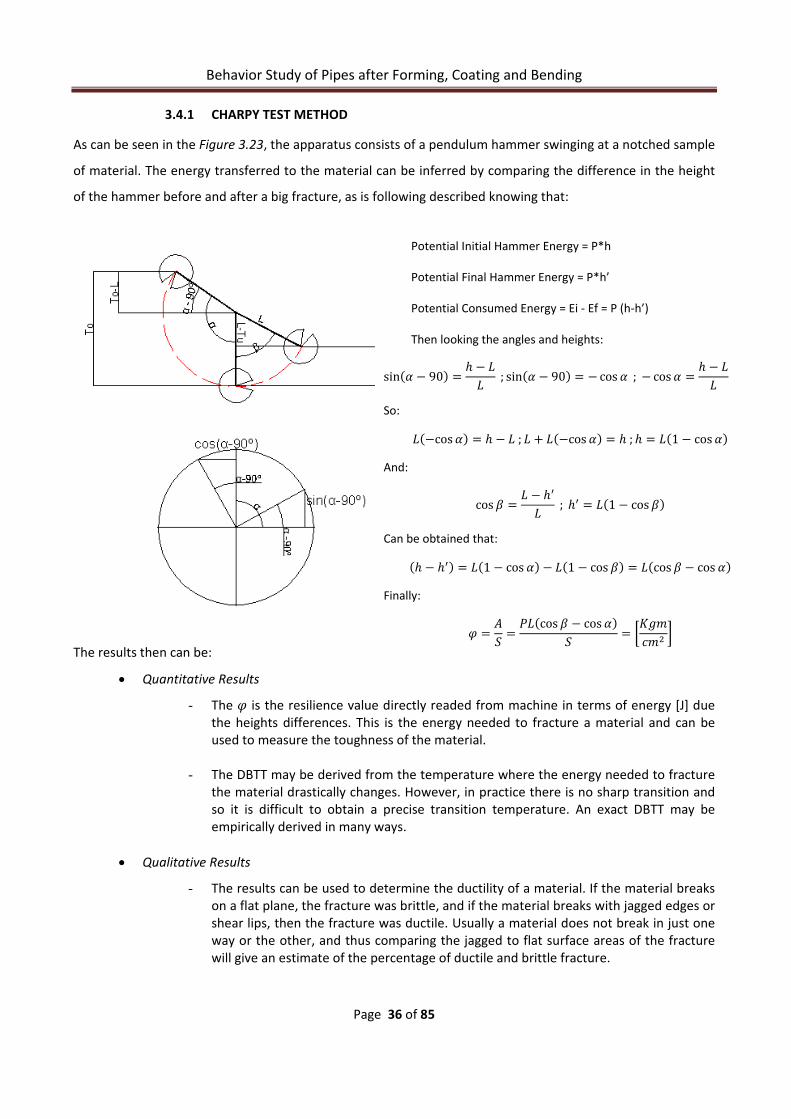
3.4.1 CHARPY TEST METHOD
As can be seen in the Figure 3.23, the apparatus consists of a pendulum hammer swinging at a notched sample
of material. The energy transferred to the material can be inferred by comparing the difference in the height
of the hammer before and after a big fracture, as is following described knowing that:
The results then can be:
• Quantitative Results
- The is the resilience value directly readed from machine in terms of energy [J] due the heights differences. This is the energy needed to fracture a material and can be used to measure the toughness of the material.
- The DBTT may be derived from the temperature where the energy needed to fracture
the material drastically changes. However, in practice there is no sharp transition and so it is difficult to obtain a precise transition temperature. An exact DBTT may be empirically derived in many ways.
• Qualitative Results
- The results can be used to determine the ductility of a material. If the material breaks on a flat plane, the fracture was brittle, and if the material breaks with jagged edges or shear lips, then the fracture was ductile. Usually a material does not break in just one way or the other, and thus comparing the jagged to flat surface areas of the fracture will give an estimate of the percentage of ductile and brittle fracture.
sin 90 ; sin 90 cos ; cos
cos ; cos ; 1 cos
cos ; 1 cos
1 cos 1 cos cos cos
cos cos
Potential Initial Hammer Energy = P*h
Potential Final Hammer Energy = P*h’
Potential Consumed Energy = Ei ‐ Ef = P (h‐h’)
Then looking the angles and heights:
So:
And:
Can be obtained that:
Finally:

Behavior Study of Pipes after Forming, Coating and Bending
Page 37 of 85
3.4.2 MECHANICAL FRACTURES AND DBTT IN CHARPY
Fracture can be defined as the mechanical separation of a solid due to the application of stress. Fractures of
engineering materials are broadly categorized as ductile or brittle [18].
DUCTILE FRACTURE
This type of fracture is characterized by high strain rates (high amount of plasticity) before the fracture. These
high strain rates can be localized near the cracks and its propagation is usually very stable, stress need to be
increased for the crack propagation.
Ductile fracture is caused by the formation and growth of the voids that eventually comprise the fracture
surface. Thus, the toughness of ductile metals is related to the factors that influence the nucleation and
growth of voids. Voids nucleate preferably at second‐phase particles, such as inclusions and precipitates and as
a result of interfacial separation, fracture of the particle or matrix separation is caused by strain concentration
near the particle.
Voids grow and coalesce by ductile tearing of the matrix. Ductile tearing resistance is a function of the strength
and ductility of the matrix. As matrix strength increases, less energy is dissipated by plastic deformation during
tearing, and toughness is reduced. Increased matrix strength also tends to activate additional void nucleation
sites. Consequently, yield strength is inversely proportional to fracture toughness
BRITTLE FRACTURE
Brittle fracture requires less energy for surface formation than ductile fracture. Lower energy fracture modes
include cleavage and intercrystalline (grain‐boundary) fracture.
Cleavage is a fracture mode in which material separation proceeds along preferred crystallographic planes
without sizable plastic deformation prior to fracture. Metals subject to cleavage usually have a large increase
in yield strength as temperature is decreased.
Cleavage occurs when the cleavage fracture stress is reached before the energy required for void formation is
exceeded. Intercrystalline fracture occurs when the cohesive strength of the grain boundary is exceeded
before cleavage or ductile fracture occurs. As matrix strength increases with decreasing temperature,
intergranular failure may occur more readily in a susceptible alloy.
A fracture surface failed in a brittle manner, shows glittering crystalline appearance because of the flat facet
produced by failure across the planes in the material.

Behavior Study of Pipes after Forming, Coating and Bending
Page 38 of 85
BDTT
Some materials exhibit brittle fracture behaviour at low temperatures rates. Above a certain limit temperature
value this behaviour turns into ductile fracture, increasing ductility values up to high values.
This temperature is well known like Brittle‐Ductile Temperature Transition (BDTT) and in steels this transition
is associated to a change in fracture mechanisms.
The rate of change from ductile to brittle behaviour depends on many parameters, including strength and
composition of the material. Because the transition occurs over a range of temperatures, it has been normal to
define a single temperature within the transition range that reflects the behaviour of the steel under
consideration.
Crystal structure is a reliable guide for qualitative prediction of temperature dependence:
• Face‐centered cubic (FCC) alloys typically exhibit high toughness throughout the ambient very low
range of temperature.
• Body‐centered cubic (BCC) alloys exhibit precipitous decreases in fracture toughness at critical
transition temperatures.
• Hexagonal close‐packed (HCP) alloys are noted for comparatively low toughness at all temperatures.
Then this transition in BCC and HCP crystal structures becomes at low temperatures, typically below ‐20ºC,
when the crystal lattice becomes closer together as the material shrinks. The closer packing of the BCC lattice
restricts the degree of shrinkage that is possible. A lower bound is reached beyond which further shrinkage is
not possible and as consequence the material has no residual elasticity remaining to absorb the impact energy
and fails in a brittle manner by cleavage between the crystal planes.
Typical CVN Fracture Energy Transition is following showed (Figure 3.21 ) with the main 3 test parameters:
Fig. 3.21 – CVN Fracture Energy Transition Curve
• USE – Upper Shelf Energy – Maximum value of the impact energy at entirely ductile material behaviour.
• LSE – Lower Shelf Energy – Low level of energy featured with cleavage fracture with low energy demands.
Entirely brittle material behaviour.
• DBTT – Ductile‐Brittle Transition Temperature – Transition zone with mixed material behaviour.

Behavior Study of Pipes after Forming, Coating and Bending
Page 39 of 85
3.4.3 EXPERIMENTAL CHARPY V‐NOTCH PROCEDURE
The delivered samples took from X65 base material have been ID as can be seen in Table 3:
Cycle Samples ID Base 3 11 16 21 49 55 60 69 70 87 91 T1 2 5 6 10 12 14 30 31 32 36 40
45 46 48 57 58 61 71 74 77 79 96 T2 15 23 24 25 27 37 42 56 62 64 65
73 75 76 80 83 88 89 92 94 95 99 T3 1 8 9 22 26 29 33 34 38 39 41
44 47 51 52 53 54 63 66 67 97 98 T4 4 7 13 17 18 19 20 28 35 43 50
59 68 72 78 81 82 84 85 86 90 93 Table 3.3 – Charpy V‐Notch Samples Identification
The Charpy samples are sawn and grinded transverse to the pipe into ISO148‐1 dimensions (Figure 3.22 &
Table 3.4) with subsize dimensions (6.7mm width). The V‐notch itself is applied by grinding.
Fig. 3.22 – Charpy sample dimensions
Dimensions Nominal dimension (mm) Tolerance (mm) Minimum dimension (mm) Maximum dimension (mm)
Length 55.0 ±0.6 54.4 55.6
Height 10.000 ±0.075 9.925 10.075
Width 10.000 ±0.11 9.89 10.11
Notch Angle 45º ±2º 43º 47º
Height below Notch 8 ±0.075 7.925 8.075
Radius 0.250 ±0.025 0.225 0.275
Notch Position 27.5 ±0.42 27.08 27.92
Table 3.4 – Charpy V‐Notch Samples Dimensions
BB
55 mm
10 mm
10 mm
45°
Radius: 0,25-mm
Section B-B

Behavior Study of Pipes after Forming, Coating and Bending
Page 40 of 85
As mentioned above the Charpy impact tests are conducted according to the standard according to ISO 148‐1:
Charpy pendulum impact test "Part1: Test method".
The tests have been done following the same procedure described in Chapter 3.3.3 also with the same
equipment and conditions. The range of temperatures used has been from 0ºC until ‐100ºC using increments
of ‐20ºC. For each temperature, 3 samples have been tested.
The tests are carried out using 750J Charpy hammer (Figure 3.23):
Fig. 3.23 – Charpy test Machine
Once the samples are tested and the results plotted as in Figure 3.21 an exponential fitting can be done in
order to quantify the energy that can be absorbed by the sample in function of the temperature.

Behavior Study of Pipes after Forming, Coating and Bending
Page 41 of 85
3.5 FEM SIMULATION
Nowadays the Finite Elements Methods simulation (FEM) has become one of the most important procedures
for multi‐physical linear and non‐linear computational cases of study.
To use any of the actual software existing for these purposes, the main starting point consists assuming the
continuum mechanical behavior which consists in a finite number of parts or elements which at the same time,
are connected with the surrounding elements by a discrete number of nodes in function of its particular
geometrical boundaries.
In this project ABAQUS® FEM software is used to study the physical behavior of a pipe under cold bending
conditions.
3.5.1 GENERAL SIMULATION STRUCTURE STUDY CASE
To perform a simulation three main steps have to be concluded as can be seen following (Figure 3.24):
Fig. 3.24 – FEM Simulations Flow Diagram
PREPROCESSING
Input file
To generate
SIMULATION
Standard/Explicit Solver
To obtain
Output
POSTPROCESSING
• Preprocessing (Abaqus/CAE)
In this stage the model is completely physically defined (Geometry, material, boundary conditions, loads, etc) close to reality.
• Simulation (Abaqus/Standard or Abaqus/Explicit)
The simulation is the stage in which Abaqus/Standard or Abaqus/Explicit solves the numerical problem defined previously. The output from a stress analysis includes displacements and stresses that are stored in binary files ready for postprocessing. It may take from seconds to days to complete a whole analysis.
• Postprocessing (Abaqus/CAE)
Once the simulation has been completed the final results can be evaluated because the displacements, stresses, or other fundamental variables have been calculated.

Behavior Study of Pipes after Forming, Coating and Bending
Page 42 of 85
3.5.1.1 STANDARD VERSUS EXPLICIT SOLVER
Abaqus® Standard is general‐purpose analysis computational software that can solve a wide range of linear
and nonlinear problems involving the static, dynamic, thermal, and electrical response of components.
For these purposes, solver solves a system of equations implicitly at each solution “increment”, it means must
iterate to determine the solution to a nonlinear problem.
The unconditionally stable implicit method will encounter some difficulties when a complicated three‐
dimensional model is considered. The reasons are as follows:
• As the reduction of the time increment continues causing divergence.
• Local instabilities cause force equilibrium to be difficult to achieve.
Abaqus® Explicit is a special‐purpose analysis solver that uses an explicit dynamic finite element formulation.
The solver tries to reach a solution forward through time in small time increments without solving a coupled
system of equations (implicit solver) at each increment. It determine the solution without iterating by
explicitly advancing the kinematic state from the previous increment
The explicit techniques are thus introduced to overcome the disadvantages of the implicit method. For the
explicit method, the CPU cost is approximately proportional to the size of the finite element model and does
not change as dramatically as the implicit method.
The problem of the explicit method is that it is conditionally stable. The stability limit for an explicit operator is
that the maximum time increment must be less than a critical value of the smallest transition times for a
dilatational wave to cross any element in the mesh.

Behavior Study of Pipes after Forming, Coating and Bending
Page 43 of 85
3.5.1.2 GENERAL SOLVERS SOLUTION DESCRIPTION [19]
The implicit procedure uses an automatic increment strategy based on the success rate of a full Newton
iterative solution method based:
(Eq. 24)
Where:
• F : Applied load. • m : Mass of the object. • a : Acceleration.
It can be rewrite more complex using constitutional equations and taking into account the nodal displacements as follows:
∆ ∆
(Eq. 25)
Where:
• Kt : Current tangent stiffness matrix. • I : Internal Force Vector. • Δu : Increment of displacement.
Implicit dynamic procedure consists step by step in the subsequently analytical steps:
ü 1
(Eq. 26)
Where:
• M : Mass matrix. • K : Stiffness matrix. • F : Vector of applied loads. • u : Displacement vector.
∆ ∆12
(Eq. 27)
And:
∆ 1
(Eq. 28)

Behavior Study of Pipes after Forming, Coating and Bending
Page 44 of 85
With:
14 1 ,
12 ,
13 0
Being α, the damping parameter by default ‐0.05 to remove the high frequency noise without having a
significant effect on the meaningful results.
In other hand, the explicit procedure is based on the implementation of an explicit integration rule along with
the use of diagonal elements mass matrices. The equation of motion for the body is integred then using an
explicit central difference integration rule being stable governed if the time increments satisfy:
∆
(Eq. 29)
Where
• : Element maximum eigenvalue.
Also the above time increment can be geometrically limited to reach the stability using the following expression:
∆
(Eq. 30)
Where:
• Le : Characteristic element dimension. • Cd : Effective dilatational wave speed of the material.
Table 3.5, summarizes and compares the main remarkable characteristics of each solver:
Item Abaqus/Standard Abaqus/Explicit
Element lib. Offers an extensive element library. Offers an extensive library of elements subset of Standard.
Analysis General and linear perturbation procedures. General procedures.
Material
models
Offers a wide range of material models. Similar to those available in Abaqus/Standard; a notable
difference is that failure material models are allowed.
Contact
formulation
Has a robust capability for solving contact problems. Has a robust contact functionality that readily solves even the
most complex contact simulations.
Solution
technique
Uses a stiffness‐based solution technique that is
unconditionally stable.
Uses an explicit integration solution technique that is
conditionally stable.
Disk space
and memory
Due to the large numbers of iterations possible in an
increment, disk space and memory usage can be large.
Disk space and memory usage is typically much smaller than that
for Abaqus/Standard.
Table 3.5 – Solvers comparison

To create a
part has to
properties c
Rigid bodie
interested i
Only the fin
• Fapu
Each one ha
this project
• Deg
The degree
Table 3.6). F
each node.
B
ny FEM simu
be firstly de
change durin
es are usuall
n the study o
nite elements
amily – Eachurposes. The
as its own fo
solid and sh
grees Of Free
es of freedom
For a stress/
Other DOF c
Behavior St
3.5.1.3 RI
ulation, all o
efined like a
ng it) or finite
ly used to m
of its physica
s need to be
h element tywhole famil
Fig
ormulation a
hell elements
edom (direct
m (DOF) are
/displacemen
can be added
udy of Pipe
GID AND DE
of the parts p
a rigid body
e element (d
model the t
al changes d
characterize
ype belongs y for stress a
g. 3.25 – Solid a
nd is prefera
s have been
tly related to
e the fundam
nt simulation
d like a varia
Fig. 3.26 – D
es after Form
Page 45 of
EFORMABLE
playing a role
(body which
deformable b
ools and th
uring the sim
ed by the fol
into a mainanalysis is sh
and shell Family
able to use in
studied to ca
o the elemen
mental varia
n the 6 degre
ble in other
DOF Diagram &
ming, Coatin
f 85
BODIES
e on it are n
h moves thro
body in funct
e finites ele
mulated proc
lowing main
n family elemhowed in the
y Finite elemen
n specific cas
arry out the
t family)
ables calcula
ees of freedo
cases of stud
DOF
1
2
3
4
5
6
& Table 3.6 – DO
ng and Bend
needed to de
ough space w
tion of consti
ements are
cess.
n aspects:
ments speci Figure 3.25:
nt types
ses accordin
simulations.
ted during t
om are the t
dy like in the
Displac
Translation in
Translation in
Translation in
Rotation abo
Rotation abo
Rotation abo
OF
ding
efine. For thi
without shap
itutional equ
used to disc
fically desig:
ng the proble
the analysis
ranslations a
ermo‐mecha
cement
n direction 1
n direction 2
n direction 3
out the 1‐axis
out the 2‐axis
out the 3‐axis
is purpose ea
pe and phys
uations).
crete the bo
ned for spe
em to solve.
(Figure 3.26
and rotations
nicals cases.
ach
ical
ody
cial
For
6 &
s at

• Num
Displaceme
the deform
The followin
(2
T
(3
Q
(4,
TE
(4
H
(8,
P
(6
• For
The elemen
forces and r
• Inte
Numerical
Gaussian q
point in eac
B
mber of nod
ents, rotation
able elemen
ng table show
ELEMENT
POINT
(1 node)
LINEAR
2 or 3 nodes)
TRIANGULAR
3 or 6 nodes)
QUADRATIC
, 8 or 9 nodes)
ETRAHEDRAL
4 o 10 nodes)
HEXAHEDRAL
20 o 27 nodes)
PRISMATICAL
6 o 15 nodes)
rmulation
nt's formulat
reactions inc
egration
techniques
uadrature fo
ch element (s
Behavior St
des
ns, temperat
nt depending
ws the finite
)
tion is refer
cluding displa
are used to
or most elem
see Chapters
udy of Pipe
tures, and th
g relate on th
e elements th
Table 3
ring to the
acements.
o integrate
ments, the s
s 3.5.1.1 & 3.
es after Form
Page 46 of
he other deg
he element g
hat can be us
ELEMENT IM
3.7 – Allowable
mathematica
various qua
software eva
.5.1.2).
ming, Coatin
f 85
rees of freed
geometry.
sed in each f
MAGE
e elements and
al theory us
antities over
aluates the
ng and Bend
dom are calc
family with it
nodes
sed to define
r the volum
material res
ding
culated only
ts nodal desc
USE LOC
POIN
LIN
SHE
SHE
VOLU
VOLU
VOLU
e the eleme
me of each e
sponse at ea
at the nodes
cription:
CATION
NTS
ES
LLS
LLS
UMES
UMES
UMES
ent's behavio
element. Us
ach integrat
s of
our,
sing
tion

Behavior Study of Pipes after Forming, Coating and Bending
Page 47 of 85
3.5.1.4 CONSISTENT SISTEM UNITS
Abaqus® software does not use specific units, however the units must be consistent throughout the model.
Regarding the different units systems, is needed to define it in the design simulation phase taking into account
this consistent criterion. Table 3.8 shows the main system units commonly used:
QUANTITY SI SI (mm) US Unit (ft) US Unit (inch) Length m mm ft in Force N N lbf lbf Mass Kg Tonne (103Kg) Slug lbf s2/ in Time s s s s Stress Pa(N/m2) MPa(N/mm2) lbf/ft2 psi (lbf/in2) Energy J mJ (10‐03J) ft lbf in lbf Density Kg/m3 tonne/mm3 slug/ft3 lbf s2/in4
Table 3.8 – Consistent units
3.5.2 PREPROCESSING AND MODEL SET‐UP
As described above in Chapter 3.5.1 the first step is the pre‐processing. Following, the FEM simulation model
of pipeline bending cold process using ABAQUS® is described. Notice that only the main features to set‐up the
model will be described, not step by step.
The whole simulation consists on several steps as happens in the real process. In order to assess the right
results, in this project will be carried out a cold bending pipe procedure to evaluate and check the final results.
Subsequently more steps and/or modifications can be included obtaining a final simulation closed to the
reality.
3.5.2.1 REAL PROCEDURE
This project is focused primarily in the cold bending process definition, using only mechanical modules of
calculation, to ensure the physics of the model, being also one of the objectives of it.
In future works, out of this project objectives, thermo‐mechanical module will be added to recreate the whole
heat induction bending process[20][21](see CD/Bending), taking into account the applied heat treatment at the
same time of the bending process.

Behavior Study of Pipes after Forming, Coating and Bending
Page 48 of 85
Cold bending process consists on placing the whole pipe in the bending machine (Figure 3.27). Diminishing the
induction coil around the pipe, the pipe passes through the induction coil at a slow, gradual rate as the
bending force applied. An exterior arm clamped to the pipe, with only rotational DOF, follows the desired
bending radius at which the pipe have to be bent. The clamp located in the beginning of the bending radius,
remains fixed all the time, to provide the necessary bending moment to deform the pipe.
Fig. 3.27 – Heat‐induction bending
The real process interested of study, is the case of 5D bend (48”x24mm of x65 Steel Grade). Being D the
diameter of the pipe, 5D fix the bending radius (R=6096mm).
To optimize FEM simulations, the case have been scaled to half all the parameters in order to reduce the
computational time costs, obtaining the same results in terms of stresses and deformations with lower times.
The main parts to complete the cold bending process in the real process required are:
• Pipe desirable to bend.
• Mobile clamp (with arm) to provide the bending.
• Fixed Clamp in future the heated area and also the beginning of the bending moment.
• Pusher to reduce or avoid frictions between machine (bending machine rollings) and pipe.

Behavior Study of Pipes after Forming, Coating and Bending
Page 49 of 85
3.5.2.2 FEM MODEL SET‐UP
PARTS DESIGN AND MESH MODULE
The 4 parts needed to define FEM definition are following showed and describing design and mesh criteria:
• PART 1 ‐ PIPE
Type of body • 3D Deformable solid
extruded body
Dimensions • Øexternal = 305mm
• Øinternal=293mm
• Length = 5000mm
Material
Definition
• Mass density = 7.85E‐
009 Tn/mm3
• Elasticity : Isotropic
• E = 210000 GPa
• Poisson’s ratio = 0.3
• Plasticity : Isotropic
• Homogenous
Mesh criteria • Approximate Global
Element Size = 50 mm
• Cordal error = 0.1mm
• Element type :
Hexahedral 8 node full
integration
PART DESCRIPTION:
Pipe is the deformable part interested to simulate to know deeply the material behavior during the bending and its final mechanical
properties.
COMMENTS:
• Plasticity is defined using experimental x65 data values from tensile test. Strain = 0.2% correspond Stress = 533.83 MPa

Behavior Study of Pipes after Forming, Coating and Bending
Page 50 of 85
• PART 2 ‐ FIXED CLAMP
Type of body • 3D Discrete solid revolved
body
Dimensions • Øexternal = 405mm
• Øinternal=295.05mm
• Length = 200mm
• Wall inclination = 135º
Material
Definition
• Mass density = 7.85E‐005
Tn/mm3
• Elasticity : Isotropic
• E = 99999999 GPa
• Poisson’s ratio = 0.3
• Plasticity : Isotropic
• Homogenous
Mesh criteria • Approximate Global Size =
27 mm
• Cordal error = 0.1mm
• Element type :
Hexahedral 8 node full
integration
DESCRIPTION:
Fixed clamp is the part where the pipe has to flow during the bending and in conjunction with the mobile clamp, and due this parte
have each 6 DOF constrained like an encastre (U1=U2=U3=UR1=UR2=UR3=0), providing the initial bending support.
COMMENTS:
• Material was scale‐up to recreate a solid discrete rigid body due software forbidden capabilities to create the model (contact
conditions and also constrain and interactions between parts).
• Density has been increased to help avoiding deformations, indeed, the rest of constants.
• Plasticity defined using experimental x65 data values from tensile test. Strain = 0.0% correspond Stress = 9999999999MPa.
• Offset of 0.05mm is needed in the inner diameter to avoid initial distortions due to overclosures.

Behavior Study of Pipes after Forming, Coating and Bending
Page 51 of 85
• PART 3 ‐ MOBILE CLAMP
Type of body • 3D Discrete solid
extruded body
Dimensions • Øexternal = 405mm
• Øinternal=295.05mm
• Length = 100mm
Material
Definition
• Mass density = 7.85E‐
010 Tn/mm3
• Elasticity : Isotropic
• E = 99999999 GPa
• Poisson’s ratio = 0.3
• Plasticity : Isotropic
• Homogenous
Mesh criteria • Approximate Global
Size = 50 mm
• Cordal error = 0.1mm
• Element type :
Hexahedral 8 node full
integration
DESCRIPTION:
Mobile clamp is the part which will gobernate the rotational movement followed by the pipe to apply the bending.
To describe the rotational movement, a reference point has been created at 1500mm from the center in X direction, being the axial
reference, and the bending radius definition.
COMMENTS:
• Material was scale‐up to recreate a solid discrete rigid body due software forbidden capabilities to create the model (contact
conditions and also constrain and interactions between parts).
• Density has been decreased to avoid inertial contributions.
• Plasticity defined using experimental x65 data values from tensile test. Strain = 0.0% correspond Stress = 9999999999MPa.
• Offset of 0.05mm is needed in the inner diameter to avoid initial distortions due to overclosures.

Behavior Study of Pipes after Forming, Coating and Bending
Page 52 of 85
• PART 4 ‐ PUSHER
Type of body • 3D Discrete solid
extruded body
Dimensions • Øexternal = 405mm
• Øinternal=295.05mm
• Length = 400mm
Material
Definition
• Mass density = 7.85E‐
010 Tn/mm3
• Elasticity : Isotropic
• E = 99999999 GPa
• Poisson’s ratio = 0.3
• Plasticity : Isotropic
• Homogenous
Mesh criteria • Approximate Global
Size = 50 mm
• Cordal error = 0.1mm
• Element type :
Hexahedral 8 node full
integration
DESCRIPTION:
Pusher is the part which will help to avoid and minimize flector moments contributions in the bending process in the tail of the pipe
describing only a linear movement.
COMMENTS:
• Material was scale‐up to recreate a solid discrete rigid body due software forbidden capabilities to create the model (contact
conditions and also constrain and interactions between parts).
• Density has been decreased to minimize inertial contributions and being a linear support guide for the tail of the pipe
imposing this movement and avoiding any other resulting movement due the bending moments and stresses.
• Plasticity defined using experimental x65 data values from tensile test. Strain = 0.0% correspond Stress = 9999999999MPa.
• Offset of 0.05mm is needed in the inner diameter to avoid initial distortions due to overclosures.

Behavior Study of Pipes after Forming, Coating and Bending
Page 53 of 85
PARTS ASSEMBLY MODULE
Once the different parts have been designed and modelled, each one needs to place all in the virtual space,
taking into account the geometrical conditions and real constrains that are also required in the initial FEM
step. For this purpose, using the assembly module, one or several instances of each part is created, rotated
and/or translated to its correct position in order to locate it with respect to each other.
The assembled model is presented below (Figure 3.28):
Fig. 3.28 – Assembled FEM model
The position constrains used in this model have been:
• Coaxial – To place coaxially the pusher and both clamps regarding the pipe.
• Face to face – To place each part in trough the Z pipe axis in the correct length position:
- Pusher – Have been placed at 1000mm from the rear face of the pipe. - Mobile clamp – Have been placed at 0mm from the front face of the pipe. - Fixed clamp – Have been placed at 0mm subsequently from the mobile clamp part.
PIPE
PUSHER
FIXED CLAMP
MOBILE CLAMP

Behavior Study of Pipes after Forming, Coating and Bending
Page 54 of 85
STEPS MODULE
FEM simulations can be divided into different steps, depending on the physical process wanted to simulate.
In the actual model, the cold bending process will be simulated creating 2 different steps:
• STEP 1 : Dynamic explicit step – Named “Gravity” during this step, gravity force is applied to ensure the
proper contacts of each part before proceeding the bending. The step time have to be enough to
affects and move each part in case of unconstrained parts, that can conclude in a model failure due
the bad constrain definition.
The defined time step is: 0.001s
• STEP 2: Dynamic explicit step – Named “Bending” during this step, all the movements are defined to
carry out the bending FEM simulation process.
This time is calculated in function of the linear velocity needed to describe a specific radius of the pipe
bending, according the following equation:
(Eq. 31)
Where: • : Angular rotational displacement [rad]. • : Angular velocity [rad/s].
Previously to the performance of this simulation, some calculations have to be taking into account. Firstly a
linear velocity of 0.45 m/s (450mm/s) for the pipe has been defined.
Using this value, and knowing that the radius of bending is R=1500mm, the angular velocity is calculated
obtaining VR2= 0.3 rad/s.
The maximum angular rotational displacement UR2, discriminating the amplitude effect, is 1.53 rad (87.6º).
And finally, the time needed for the simulation can be solved, using the equation 31:
1.530.3
5.1

Behavior Study of Pipes after Forming, Coating and Bending
Page 55 of 85
INTERACTIONS
Although the parts have been assembled, more information is needed for the software to define the
interactions between the different meshed surfaces during the simulation. To define it master‐slave contact
pairs have to be defined for all the surfaces in contact with each other.
Abaqus provides two algorithms to model contact interactions: The general contact interactions allow
defining contact between many or all regions of the model with a single interaction and surface‐to‐surface
contact interactions describe contact between two deformable surfaces or between a deformable surface and
a rigid surface.
In this model, surface‐to‐surface contact definition has been used. It requires the definition of all the surfaces
in contact with each other (Figure 3.29). The master and the salve surfaces should be defined for each
interaction set, being considered the fixed clamp inner surface as the “master surface” while considering the
outer pipe surface as the “slave surface”.
Fig. 3.29 – Assembled FEM model
PIPE ‐ SLAVE
FIXED CLAMP ‐ MASTER

Behavior Study of Pipes after Forming, Coating and Bending
Page 56 of 85
Also the kinematic constrain formulation has to be applied using “kinematic contact” or “penalty contact”:
• Kinematic contact ‐ First advances the kinematic state of the model into a predicted configuration
without considering the contact conditions. After, the slave nodes in the predicted configuration that
are penetrating the master surfaces are defined and the depth of each slave node’s penetration, the
mass associated with it, and the time increment are used to calculate the resisting force required to
oppose penetration
• The penalty contact algorithm searches for slave node penetrations in the current configuration.
Contact forces that are a function of the penetration distance are applied to the slave nodes to oppose
the penetration, while equal and opposite forces act on the master surface at the penetration point
The penalty contact algorithm results in less severe enforcement of contact constraints than the kinematic
contact algorithm, but the penalty algorithm allows for treatment of more general types of contact, being used
for this model. Also, a very important aspect is that Coulomb friction is defined like μ=0 in this contact pair, to
minimize the pipe distortion due frictional effects once is flowing through the fixed clamp.

Behavior Study of Pipes after Forming, Coating and Bending
Page 57 of 85
CONSTRAINS
Despite interactions in the whole contact surfaces is the commonly way to perform a FEM model, in this case
several contact problems have appeared difficulting it.
Due the intrinsical characteristics of the simulation, however, an alternative way has been defined to provide a
successfully method to define the rest of the contacts using constrains options.
MOBILE CLAMP
To describe properly and control the mobile clamp rotational movement, a reference point with an offset of
the desired bending radius (R=1500mm) respect the axial pipe coordinates (Y axis) straight on the X axis, has
been created as can be see following (Figure 3.30):
Fig. 3.30 – Mobile Clamp Constrains
As can be seen in this reference point (RP), the angular velocity DOF (VR2‐Red arrow in figure 3.29) is applied,
so a coupling constrain involving RP and all the nodes from the mesh of the mobile clamp is applied forcing all
its nodes to follow exactly the same movement of the RP, defining the bending rotational movement.
This rotational movement only affects the mobile clamp, regarding that no interaction between the mobile
clamp and the pipe has been yet create. For this reason another constrain is required to “weld” the nodes of
the inner clamp surface and the pipe outer surface.
VR2

Behavior Study of Pipes after Forming, Coating and Bending
Page 58 of 85
Figure 3.31 shows a tied constrain between the surfaces which is defined recreating a “weld” condition and
guarantying that pipe is following the movement of the mobile clamp.
Fig. 3.31 – Mobile Clamp & Pipe Tie and Coupling Constrains
PUSHER
Same procedure is used to define the linear translational pusher movement (Figure 3.32), creating firstly its
own RP and after a coupling constrain between RP and the nodes finishing with another constrain to “weld”
coupling both interacting surfaces.
Fig. 3.32 – Pusher & Pipe Tie and Coupling Constrains

Behavior Study of Pipes after Forming, Coating and Bending
Page 59 of 85
AMPLITUDE ASSIGNEMENTS
In order to avoid accelerations problems, product to change the velocity (from 0 mm/s until X mm/s) value in
the same time step and due the partial derivation used by the solver for each increment of time, the solver can
reach an infinite or very high final value, which may lead to unexpected time and force instabilities.
To avoid the instabilities, is very helpfully the application of an initial smooth step within the main step in
gravity as in bending.
This initial smooth step is applied where the velocity increases gradually till the required bending velocity and
then, a constant velocity step is employed. Finally, a deceleration step is applied towards the end of the
bending process until a velocity equal to zero is reached.

Behavior Study of Pipes after Forming, Coating and Bending
Page 60 of 85
4 RESULTS AND DISCUSSION
4.1 SAMPLING AND COATING RECREATION
The recorded real temperature evolution of the samples during the coating simulation process in the furnace is following plotted (Figure 4. 1 & Figure 4. 2):
0 200 400 600 800 1000 1200 1400 1600 1800 200050
60
70
80
90
100
110
120
130
140
150
T1 and T2 140ºC Heat CycleTe
mpe
ratu
re (º
C)
Time (s)
T1-30s T2-300s
Fig. 4. 1 – T1 and T2 Heat Treatment
0 500 1000 1500 2000 2500 3000 3500100110120130140150160170180190200210220230240250260
T3 and T4 245ºC Heat Cycle
Tem
pera
ture
(ºC
)
Time (s)
T3-30s T4-300s
Fig. 4. 2 – T3 and T4 Heat Treatment
Due the nature of the furnace, the maximum value of temperature that can be reached is 245ºC, and taking into account the heating power high values of time are needed to reach the desired temperature in the samples longer than the applied in the coating processes if quenched is applied (Table 1.4 & CD/COATINGS).
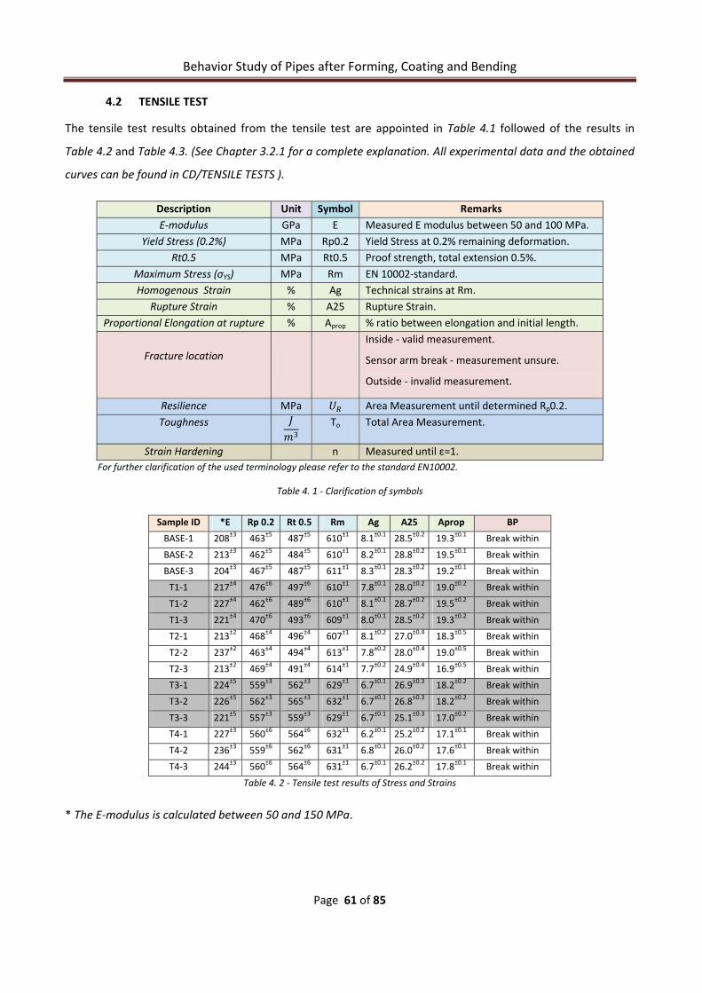
Behavior Study of Pipes after Forming, Coating and Bending
Page 61 of 85
4.2 TENSILE TEST
The tensile test results obtained from the tensile test are appointed in Table 4.1 followed of the results in
Table 4.2 and Table 4.3. (See Chapter 3.2.1 for a complete explanation. All experimental data and the obtained
curves can be found in CD/TENSILE TESTS ).
Description Unit Symbol Remarks E‐modulus GPa E Measured E modulus between 50 and 100 MPa.
Yield Stress (0.2%) MPa Rp0.2 Yield Stress at 0.2% remaining deformation. Rt0.5 MPa Rt0.5 Proof strength, total extension 0.5%.
Maximum Stress (σYS) MPa Rm EN 10002‐standard.Homogenous Strain % Ag Technical strains at Rm.
Rupture Strain % A25 Rupture Strain.Proportional Elongation at rupture % Aprop % ratio between elongation and initial length.
Fracture location
Inside ‐ valid measurement.
Sensor arm break ‐ measurement unsure.
Outside ‐ invalid measurement.
Resilience MPa Area Measurement until determined Rp0.2. Toughness
To Total Area Measurement.
Strain Hardening n Measured until ε=1.For further clarification of the used terminology please refer to the standard EN10002.
Table 4. 1 ‐ Clarification of symbols
Sample ID *E Rp 0.2 Rt 0.5 Rm Ag A25 Aprop BP
BASE‐1 208±3 463±5 487±5 610±1 8.1±0.1 28.5±0.2 19.3±0.1 Break within
BASE‐2 213±3 462±5 484±5 610±1 8.2±0.1 28.8±0.2 19.5±0.1 Break within
BASE‐3 204±3 467±5 487±5 611±1 8.3±0.1 28.3±0.2 19.2±0.1 Break within
T1‐1 217±4 476±6 497±6 610±1 7.8±0.1 28.0±0.2 19.0±0.2 Break within
T1‐2 227±4 462±6 489±6 610±1 8.1±0.1 28.7±0.2 19.5±0.2 Break within
T1‐3 221±4 470±6 493±6 609±1 8.0±0.1 28.5±0.2 19.3±0.2 Break within
T2‐1 213±2 468±4 496±4 607±1 8.1±0.2 27.0±0.4 18.3±0.5 Break within
T2‐2 237±2 463±4 494±4 613±1 7.8±0.2 28.0±0.4 19.0±0.5 Break within
T2‐3 213±2 469±4 491±4 614±1 7.7±0.2 24.9±0.4 16.9±0.5 Break within
T3‐1 224±5 559±3 562±3 629±1 6.7±0.1 26.9±0.3 18.2±0.2 Break within
T3‐2 226±5 562±3 565±3 632±1 6.7±0.1 26.8±0.3 18.2±0.2 Break within
T3‐3 221±5 557±3 559±3 629±1 6.7±0.1 25.1±0.3 17.0±0.2 Break within
T4‐1 227±3 560±6 564±6 632±1 6.2±0.1 25.2±0.2 17.1±0.1 Break within
T4‐2 236±3 559±6 562±6 631±1 6.8±0.1 26.0±0.2 17.6±0.1 Break within
T4‐3 244±3 560±6 564±6 631±1 6.7±0.1 26.2±0.2 17.8±0.1 Break within
Table 4. 2 ‐ Tensile test results of Stress and Strains
* The E‐modulus is calculated between 50 and 150 MPa.

Behavior Study of Pipes after Forming, Coating and Bending
Page 62 of 85
Following a comparison of the average tensile test results is following plotted (Figure 4. 3 & Figure 4. 4):
BASE T1 T2 T3 T4 --0
50
100
150
200
250
300
350
400
450
500
550
600
650
Average Stresses ComparisonSt
ress
[MPa
]
Sample Condition ID
Rp0.2 Rt0.5 Rm
Fig. 4. 3 – Average Stresses Comparison
BASE T1 T2 T3 T40
5
10
15
20
25
30
35
Average Strains Comparison
Stra
in %
Sample Condition ID
Ag% A25 Aprop
Fig. 4. 4 – Average Strains Comparison

Behavior Study of Pipes after Forming, Coating and Bending
Page 63 of 85
Looking stresses (Table 4.2 and Figure 4.3), heated simulations T1 and T2 do not exhibit any significant change
in stress compared to the base material. Heated simulations T3 and T4 however show significant higher
ultimate tensile strength (Rm) and yield strength (Rp0.2 and Rt0.5).
Taking into account that long times have been needed to reach the desired temperature, as can be seen in
Figures 4.1 & 4.2, the time has no influence in the results, being the temperature the main factor that alters
the mechanical properties.
The E has no significant change in any case, because of the ratio that reflect (stress‐strain slope in the elastic
region) is almost the same despite tends to increase in T3 and T4 heated simulations. Taking into account that
the values have been obtained using a range of stress between 50 and 150 MPa, is means that the higher slope
the lower strain is obtained.
On the other hand, Figure 4.4, shows clearly that the rupture strain (A25) is lower for simulations T3 and T4
than for the Base material and both T1 and T2 heated simulations.
The ductility (APROP) tends to decrease in heated simulations T3 and T4 compared to Base material, which has
the greater values, and also with T1 and T2 heated simulations, which have closed lower values than the last
one.
Sample ID UR To n Rt0.5/Rm
BASE‐1 1.025±0.010 155.8±0.6 0.61 0.79±0.30
BASE‐2 0.964±0.010 157.2±0.6 0.61 0.79±0.30
BASE‐3 0.969±0.010 154.7±0.6 0.61 0.79±0.30
T1‐1 1.008±0.015 152.3±0.4 0.65 0.81±0.35
T1‐2 1.005±0.015 156.9±0.4 0.63 0.80±0.35
T1‐3 0.922±0.015 155.2±0.4 0.57 0.81±0.35
T2‐1 0.915±0.018 146.8±0.2 0.39 0.82±0.25
T2‐2 0.948±0.018 153.7±0.2 0.62 0.81±0.25
T2‐3 0.981±0.018 137.5±0.2 0.68 0.79±0.25
T3‐1 1.277±0.014 150.5±0.8 0.72 0.89±0.20
T3‐2 1.258±0.014 149.0±0.8 0.66 0.89±0.20
T3‐3 1.237±0.014 139.9±0.8 0.62 0.88±0.20
T4‐1 1.254±0.021 140.0±0.4 0.61 0.89±0.35
T4‐2 1.254±0.021 146.0±0.4 0.72 0.89±0.35
T4‐3 1.228±0.021 148.0±0.4 0.72 0.89±0.35
Table 4. 3 – Extracted results from Tensile Test
In Table 4.3 the values of the UR are higher than the base material and T1 and T2 heated simulations so more
energy can be absorbed in the elastic region. In other hand, although do not have significant changes, tends to
decrease in T3 and T4 heated simulations. It means that the total area under the stress‐strain curve is less due
the higher stress values and lower A25 values.

Behavior Study of Pipes after Forming, Coating and Bending
Page 64 of 85
The n obtained values from the total of tested samples are higher than the standard values for x65 steel grade
(between 0.40 and 0.45). As explained in Chapter 3.2.1 the higher the value is the higher is the applied strain in
the material. These higher values show that in the UOE process, the tested area is prestrained.
Prestrain means introduce plasticity in the material, so the Rp0.2 is passed. Regarding the UOE process (see
Chapter 1.3.3)[3] in the second process step forms the U, on the down of the U, the material need to resists the
stresses once the material is drawing and conforming the U adapting to the punch geometry. In a previous
FEM simulation of the UOE process the U step forming was simulated as can be seen in the following
sequences (Figure 4. 5):
Fig. 4. 5 – FEM U Step Process Sequence
As can be seen in 4th sequence, the Von‐Misses stresses reach values up to 70000psi (482MPa) approximately,
so the material has been deformed plastically and n value is higher than standard values for x65 steel grade.
1ST Sequence 2ND Sequence 3RD Sequence
4TH Sequence

Behavior Study of Pipes after Forming, Coating and Bending
Page 65 of 85
It important to notice, that the UOE process begins using plates of steel. This plates are also Thermo‐
Mechanically Cooled Processed (TMCP) in order to control the mechanical properties taking into account the
mainly grain boundary preferably misorientation control the grain size and the steel constituents such as
Acicular Ferrite (AF), Granular Bainite (GB), Martensite‐Austenite (MA), etc. that is strongly dependent of the
steel grade. As the steel plates are finally laminated in TMCP, have been demonstrated different mechanical
properties comparing the longitudinal direction versus the transverse direction. Despite several research
projects are also studying this effects, nowadays all of them reflects that the worst mechanical properties are
in the transverse direction and strain hardening could be summed being, then not only UOE process the single
way to introduce strain.
Pipe steels have also different chemical constituents, and once the steel is melted and cooled, the hardening
can increase due the precipitation of carbides, nitrides, etc. which remains pinned in the ferritic matrix of the
steel. Also, the strain applied in the UOE process increases the number of dislocations in the material because
of the relative lattice movement of the grains.
The temperatures applied in the simulated heat treatment are so far from the recrystallization temperatures
of the steels, typically 0.4TMELTING (above 550ºC), and it means that the material has not enough energy to
create new equiaxial grains explaining the reason of the decrease in the strain rates showed in Table 4.2 and
Figure 4.4.
In other hand, the greater value of heat is enough to provide energy to unpinned some of dislocations,
increasing the mechanical properties (Rp0.2 and Rt0.5) as appear in the Table 4.2 and Figure 4.3. Due the long
time needed to reach the temperature using this furnace, any significant difference between T3 and T4 heated
simulations appear.
Finally, in the Table 4.3 a ratio between Rt0.5/Rm is presented. This ratio is very important in pipelines,
defined also in the Standard API 5L. This value is very important in the design criteria of the pipelines because
have a significant relation with the buckling in pipes. As higher is the value, less is the possibility of buckling
failure and longer the length of the pipe depending on the over collapse pressure. According to the API
definitions, minimum values of 0.8 guaranties high standards of applications.
Due the increase of the mechanical properties, in T3 and T4 heated simulations, this ratio is increased.

Behavior Study of Pipes after Forming, Coating and Bending
Page 66 of 85
4.3 HEAT TRANSFERS IN CHARPY V_NOTCH TEST
4.3.1 ANALYTICAL PROCEDURE
For analytical procedure, has been needed to find and extrapolate some values of different constants and
apply them into the required equations to obtain the values of convective factor h.
The data treatment and results will be presented in the CD/CSTT/CSTT.xls.
The analytical procedure will be focused in the two mechanisms described above, natural and forced
convection, due to while the Charpy experimental test, the sample is firstly homogeneously cooled into a
fridge, and then the sample is picked out and placed into the test Charpy machine. During this procedure is
considered that:
- First stage – Forced convection is acting because the sample is picked and placed in the test machine.
In this stage a constant velocity of 2m/s is assumed during 5 seconds.
- Second stage – Natural convection is acting because the sample has been placed in the machine, and
remains waiting for the hammer impact. Initially is assumed that the contact area is very small, and
conduction effects can be neglected. The approximate time is around 2 seconds.
The sum of the two mechanisms, determines the heat transfer of the sample in the system and knowing it the
final temperature in function of time can be calculated, taking into account the initial temperature of the
sample, because of the temperature dependence of different physical magnitudes involved in this
thermodynamic study.
4.3.1.1 ANALYTICAL PROCEDURE FOR NATURAL CONVECTION
To solve the heat transfer equation, is needed to know the B value. This parameter includes the h value and to
know it, previously the Grashof dimensionless number has to be calculated according to the equation:
∆
For this equation be assume that:
•
• 12.5 10
• : Kinematic viscosity is function of the temperature. As can be seen in the Annex1‐Figure 13 according standard values, the evolution has been fitted to obtain an equation for a complete range of temperatures:

Behavior Study of Pipes after Forming, Coating and Bending
Page 67 of 85
The obtained 4th polynomial fitted equation is:
4.565 7.2098 1.1138 0.0865 13.318
(Values can be found in CD/CSTT/time‐temp dependence.xls; sheet “kine visco AIR”)
For each temperature, from ‐160ºC to 20ºC, fixing temperature increments with value of 10ºC, and using the
previous equation, Gr dimensionless number have been found.
Same procedure has been done to find the Prandtl dimensionless number (Pr), according to the equation:
To obtain fitted values to determine, for each incremental step of temperature, the values of Cp and k (see
CD/CSTT/Air K Fitting & Air Cp Fitting).
The obtained polynomial equations are:
Cp 4.3207 1.16296 1.00575
k 2.72436 0.07477 24.01686
(Values can be found in CD/CSTT/time‐temp dependence.xls; sheets “Cp AIR” and “K Air” respectively and
CD/CSTT/Cp Air Fitting)
Once Pr is obtained (see CD/CSTT/time‐temp dependence.xls; sheet “Pr”), the product of Gr*Pr dimensionless
numbers, is the Rayleigh dimensionless number which determine the type of flow regime.
As can be seen in CD/CSTT/time‐temp dependence.xls; sheet “h Natural Conv f(T)” the maximum results is
1,112E+05, being less than 109, concluding that in the case of the maximum difference between temperatures
(‐160ºC to 21ºC), the flow regime is laminar. The constants can be fixed, according standards, to calculate the
Nu dimensionless number and finally obtain the h value for each incremental step of temperature.
Finally using the equation of the energetic balance, the B parameter is obtained, for each step. The Cp for X65
steel has been fitted (see CD/CSTT/time‐temp dependence.xls; sheet “Cp Steel”), to obtain an equation to
define its evolution in function of temperature (CD/CSTT/Cp Steel Fitting):
0.44 450
Where: y represents Cp of the steel and x the temperature [J/KgK].

Behavior Study of Pipes after Forming, Coating and Bending
Page 68 of 85
Fixing the initial temperature Ti, the final temperature in function of time can be determined. The results are plotted in the Figure 4. 6:
0.1 1 10 100 1000-160-150-140-130-120-110-100-90-80-70-60-50-40-30-20-10
01020
Natural Convection T(t) Evolution
Tem
pera
ture
[ºC
]
Time [s]
T(-160ºC) T(-150ºc) T(-140ºC) T(-130ºC) T(-120ºC) T(-110ºC) T(-100ºC) T(-90ºC) T(-80ºC) T(-70ºC) T(-60ºC) T(-50ºC) T(-40ºC) T(-30ºC) T(-20ºC) T(-10ºC) T(0ºC)
Fig. 4. 6 – Temperature evolution in function of time for each incremental step of temperature for natural convection
The main thermodynamics behaviors in case of natural convection that can be observed are:
- Long times are needed to reach the room temperature, so the heat transfer is very small because of h.
- In function of initial temperature, the temperature versus time evolution is different, however, in the
initial times, from 0 to 20 seconds, the behavior is strongly similar in each initial temperature case.

Behavior Study of Pipes after Forming, Coating and Bending
Page 69 of 85
In Figure 4. 7 the initial evolution is zoomed showing the temperature evolution of the sample:
0.1 1 10-160-150-140-130-120-110-100-90-80-70-60-50-40-30-20-10
01020
Natural Convection T(t) Evolution
Tem
pera
ture
[ºC
]
Time [s]
T(-160ºC) T(-150ºc) T(-140ºC) T(-130ºC) T(-120ºC) T(-110ºC) T(-100ºC) T(-90ºC) T(-80ºC) T(-70ºC) T(-60ºC) T(-50ºC) T(-40ºC) T(-30ºC) T(-20ºC) T(-10ºC) T(0ºC)
Fig. 4. 7 – Plotted zoom of temperature evolution for natural convection
4.3.1.2 ANALYTICAL PROCEDURE FOR FORCED CONVECTION
In case of forced convection, the same steps have been followed. In this case, but, the influence of the velocity
is the main factor which permit increase the h value, and consequently the heat transfer in the system.
For this case, a velocity of 2.5m/s has been considered as the mean velocity required moving the sample from
the fridge to the Charpy test machine, assuming that the velocity is not constant in all the procedure. This step
needs around 5 seconds.
Using previous data fitted, when is required, the Re dimensionless number has been calculated for each
increment of temperature (see CD/CSTT/time‐temp dependence.xls; sheet “h Forced Conv f(T)”).

Behavior Study of Pipes after Forming, Coating and Bending
Page 70 of 85
Then considering a rectangular case and the flux situation as described in the Figure 4. 8 for the cross section,
the standard constants to be taken into account, can be seen below:
Fig. 4. 8 – Forced convection flux for rectangular cross section definition
• C = 0.227 • m = 0.731
•
As described previously and using the equation for cylinders of other cross sections different than circular
cylinders, the Nu dimensionless number for each step of temperature have been found, and finally the h value
for forced convective mechanism.
Fixing the initial temperature Ti, the final temperature in function of time can be determined, which results are
plotted in the Figure 4. 9:
0.1 1 10 100 1000-160-150-140-130-120-110-100
-90-80-70-60-50-40-30-20-10
01020
Forced Convection T(t) Evolution
Tem
pera
ture
[ºC
]
Time [s]
T(-160ºC) T(-150ºc) T(-140ºC) T(-130ºC) T(-120ºC) T(-110ºC) T(-100ºC) T(-90ºC) T(-80ºC) T(-70ºC) T(-60ºC) T(-50ºC) T(-40ºC) T(-30ºC) T(-20ºC) T(-10ºC) T(0ºC)
Fig. 4. 9 – Temperature evolution in function of time for each incremental step of temperature for forced convection
Flow direction

Behavior Study of Pipes after Forming, Coating and Bending
Page 71 of 85
The main thermodynamics behaviors in case of forced convection that can be observed are:
• The times needed to reach the room temperature are quite lower than in natural convection. It can be deduced that the heat transfer is higher due the effects of the friction between fluid and the sample.
• In function of initial temperature, the temperature versus time evolution is different, in this case, in the graph appears different behaviors for each initial temperature.
• The initial time, is very important due that in few seconds, the heat transfer is very high, and the sample wins heat very fast from the air.
Figure 4. 10 shows the plotted graph zoomed in the initial times showing more clearly the temperature
evolution of the sample in forced convection:
0.1 1 10-160-150-140-130-120-110-100-90-80-70-60-50-40-30-20-10
01020
Forced Convection T(t) Evolution
Tem
pera
ture
[ºC
]
Time [s]
T(-160ºC) T(-150ºc) T(-140ºC) T(-130ºC) T(-120ºC) T(-110ºC) T(-100ºC) T(-90ºC) T(-80ºC) T(-70ºC) T(-60ºC) T(-50ºC) T(-40ºC) T(-30ºC) T(-20ºC) T(-10ºC) T(0ºC)
Fig. 4. 10 – Plotted zoom of temperature evolution in function of time for each incremental step of temperature for forced convection

Behavior Study of Pipes after Forming, Coating and Bending
Page 72 of 85
4.3.2 EXPERIMENTAL PROCEDURE
Following, the temperature recorded temperature evolution is plotted (Figure 4. 11):
100 1000 10000-100
-90
-80
-70
-60
-50
-40
-30
-20
Experimental Temperature (t) Evolution
Tem
pera
ture
[ºC
]
Time [ms]
100ºC 80ºC 60ºC 40ºC 20ºC
Fig. 4. 11 –Experimental Temperature vs. Time dummy evolution
Summarizing the recorded evolution of temperature in function of the time, as specified above, Table 4.4
shows the main important obtained data:
T[ºC] T1 (in freezer)[ºC] T2 (hit) [ºC] ΔT [ºC]‐20 ‐19.9±0.1 ‐19.1±0.1 0.8±0.1
‐40 ‐39.7±0.1 ‐38.7±0.1 1.0±0.1
‐60 ‐59.4±0.1 ‐58.1±0.1 1.3±0.1
‐80 ‐79.5±0.1 ‐78.0±0.1 1.5±0.1
‐100 ‐99.0±0.1 ‐97.2±0.1 1.8±0.1
Table 4. 4 ‐ Recorded data summary
Where:
• T: Real temperature expected to reach. • T1 : Real dummy temperature after 30 minutes. • T2 : Real dummy temperature once the hammer impact. • ΔT : Increment of temperature between T2‐T1.
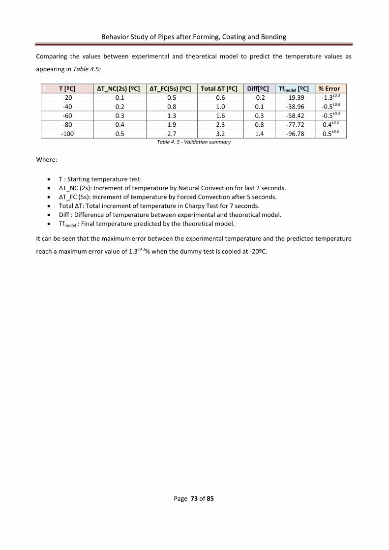
Behavior Study of Pipes after Forming, Coating and Bending
Page 73 of 85
Comparing the values between experimental and theoretical model to predict the temperature values as
appearing in Table 4.5:
T [ºC] ΔT_NC(2s) [ºC] ΔT_FC(5s) [ºC] Total ΔT [ºC] Diff[ºC] Tfmodel [ºC] % Error ‐20 0.1 0.5 0.6 ‐0.2 ‐19.39 ‐1.3±0.3 ‐40 0.2 0.8 1.0 0.1 ‐38.96 ‐0.5±0.3 ‐60 0.3 1.3 1.6 0.3 ‐58.42 ‐0.5±0.3 ‐80 0.4 1.9 2.3 0.8 ‐77.72 0.4±0.3 ‐100 0.5 2.7 3.2 1.4 ‐96.78 0.5±0.3
Table 4. 5 ‐ Validation summary
Where:
• T : Starting temperature test. • ΔT_NC (2s): Increment of temperature by Natural Convection for last 2 seconds. • ΔT_FC (5s): Increment of temperature by Forced Convection after 5 seconds. • Total ΔT: Total increment of temperature in Charpy Test for 7 seconds. • Diff : Difference of temperature between experimental and theoretical model. • Tfmodel : Final temperature predicted by the theoretical model.
It can be seen that the maximum error between the experimental temperature and the predicted temperature
reach a maximum error value of 1.3±0.3% when the dummy test is cooled at ‐20ºC.

Behavior Study of Pipes after Forming, Coating and Bending
Page 74 of 85
4.4 CHARPY V‐NOTCH IMPACT TEST
The results of CVN tests are shown following (Figure 4. 12 until Figure 4. 15):
Fig. 4. 12 –T1 CVN Results
Fig. 4. 13 –T1 CVN Results

Behavior Study of Pipes after Forming, Coating and Bending
Page 75 of 85
Fig. 4. 14 –T3 CVN Results
Fig. 4. 15 –T1 CVN Results

Behavior Study of Pipes after Forming, Coating and Bending
Page 76 of 85
Table 4.6 summarizes the main values obtained from CVN Impact test:
T1 T2 T3 T4 USE [J] 242 212 238 313
LSE [J] 0 14 9 5
DBTT [ºC] ‐54 ‐53 ‐48 ‐35 Table 4. 6 – CVN Summarized Results
As can be observed in Table 4.6 the USE has a notably increase in T4 heated simulation. The rest of the heated
simulations do not show any significant result of the ductility behavior of the material. It can be explained due
the higher temperature and also higher time applied to the sample due to allow the material to unpin more
dislocations and consequently the material can absorb more impact energy.
DBTT depends upon a number of factors, including the microstructure, the composition, the loading rate, and
the test environment. The strain plays an important role one it, the higher the strain rate the higher the DBTT.
In this heated simulations, the temperature was below of recrystallization temperature, so no effects on strain
can be expected, no changes in the dislocations global amount density. However, at higher temperatures and
times, the unpinned number of dislocations is higher, than at lower temperatures and treatment times, so it
can be seen in DBTT that tends to decrease at higher temperatures and also treatment times (T1DBTT = ‐54ºC
and T4DBTT = ‐35ºC).

Behavior Study of Pipes after Forming, Coating and Bending
Page 77 of 85
4.5 FEM SIMULATION
POSTPROCESSING
As showed in Figure 3.24 the last step once the FEM simulation is finished consists on the postprocessing
analysis of the virtual obtained results.
Following the main steps of cold bending FEM simulation are showed (Figure 4. 16 until Figure 4.18):
Fig. 4. 16 –Bending step at t=0s.
Fig. 4. 17 –Bending step at t=2.1s.
Fig. 4. 18 –Bending step finished.

Behavior Study of Pipes after Forming, Coating and Bending
Page 78 of 85
It can be observed how the pipe is bended according the rotational movement described by the mobile clamp.
The pusher helps the pipe to flow according rotational velocity and also avoid bending moments of the pipe
tail.
The fixed clamp then, is the part when the pipe starts to bend remaining encastred during the whole
simulation.
FEM software has different options to analyze the resultant simulated body. Figure 4.19 & Figure 4.20 shows
the Von‐Misses stresses results:
Fig. 4. 19 –Intrados Pipe Von‐Misses Stresses
Fig. 4. 20 –Extrados Pipe Von‐Misses Stresses
Pictures show stresses corresponding to the compression and tension stresses due the cold bending process.

Behavior Study of Pipes after Forming, Coating and Bending
Page 79 of 85
From previous experimental test, same case was tested to know the mechanical properties of the material as
can be seen in the following Figure 4.21. Using a software option “query information at integration node” Von‐
Misses stresses values from the FEM simulation can be known accurately in the same regions (values obtained
from the simulation are showed together with the Figure 4.21. Green boxes correspond to the cases that great
accuracy within the results has obtained; Red boxes correspond to results with a discrepancy of ± 25MPa that
are assumed like bad results):
Fig. 4. 21 –Pipe Experimental Stresses and FEM Von‐Misses Stresses
As can be seen, stresses values in section 1 and 2 are closed to the experimental values.
Closed to Section 3 the results show higher discrepancies, and section 4 due the use of not rigid tool to define
the mobile clamp, the obtained results cannot be taking into account.

Behavior Study of Pipes after Forming, Coating and Bending
Page 80 of 85
It can also be plotted the final strain state of the pipe after cold bending Figure 4.22 and Figure 4.23:
Fig. 4. 22 –Extrados Logarithmic Strain
Fig. 4. 23 –Intrados Logarithmic Strain
The Figure 4.22 shows higher strain values due the extension of the material (extrados). On the other hand
Figure 4.23 shows lower strain values in the compression zone (intrados).
Strain values cannot be contrasted neither previous FEM validated model nor experimental test.

Behavior Study of Pipes after Forming, Coating and Bending
Page 81 of 85
5 CONCLUSIONS
The study of the coating processes has been done, and time and temperature range (minimum and maximum)
has been also fixed.
Tensile tests have demonstrated that the UOE forming process, increase the strain in the pipe compared to
base material. They also have showed the influence of strain in the mechanical properties of the x65 steel
grade with and without the application of the coatings heated simulations, increasing the yield strength
(Rp0.2) and reducing the rupture strain (A25).
Charpy V‐Notch impact tests have demonstrated the behaviour of the x65 steel grade with heated simulations
under the application of dynamical loads showing how steel tends to increase the upper shelf energy (USE)
and decrease the brittle‐ductile temperature transition (BDTT), winning in ductility but loosing however in the
range of in service temperature.
Charpy V‐Notch Samples Temperature Test have provide a better understanding of heat transfer in this type of
steel, and a analytical procedure have been defined and parameterized in order to use with other steel data.
This model has also been validated using experimental measurement and is helpfully in order to guarantee the
quality of Charpy V‐Notch experimental standards.
Finite Element Method (FEM) simulation of the cold bending pipe process have been done and also have been
parameterized in order to be able to simulate different bending conditions changing some parameters such
material, bending radius, thickness of the pipe, etc.

Behavior Study of Pipes after Forming, Coating and Bending
Page 82 of 85
6 FUTURE WORKS
The effects of pre‐strain in the base material need to be strongly considered due the direct impact on the mechanical properties in the pipelines steel grades.
Firstly, a better knowledge of the actual strain state of pipe circumferentially around itself has to be studied. After and once defined the actual strain ratios due the UOE forming process, a complete test program will include the application of strain into the samples from base material until strain % higher than the obtained in the pipe forming process.
All these samples will need to be heat treated more closely to the real process, in terms of heat application times.
All this tests can be carried out using the Gleeble simulator, a thermo‐mechanical machine that can apply strain and controlled heated program.
Tensile and Charpy V‐Notch tests will bring a deep knowledge of the mechanical properties of the steel due the coating recreations.
The FEM simulations need to be validated so experimental tests are required in order to ensure it. In other hand FEM simulations need to be coupled with the thermo‐mechanical module to recreate and simulate the hot bending procedure.
Once the FM model will be validated, a parametric study will be carried out to predict the mechanical and/or thermo‐mechanical behavior of the pipe under bending conditions in function of different parameters such: changes in thickness, in the material, in the heat treatment, in the bending radius.
7 ENVIRONMENTAL ASPECTS
The most remarkable environmental effect in the present project is the use of FEM simulation. Once the FEM
model will be finished and validated, the final mechanical properties will be predicted. It means less amount of
material, so can be translated directly into less contamination and energy save because of the less necessity to
create the pipe and samples for testing.

Behavior Study of Pipes after Forming, Coating and Bending
Page 83 of 85
8 COSTS
The costs of the present project have been divided in specific budgets:
BUDGET 1 CONCEPT: FEM Software
REF. DESIGNATION UNIT PRICE UNIT (€) AMOUNT TOTAL (€)
1.1 Abaqus ® 6.9.1 License Ut. 25.000 1 25.000
1.2 Abaqus ® 6.9.1 Maintenance Ut. 7.000 1 7.000
1.3 Computational equipment
- PC - Operative System
Ut.
2.500 1 2.500
Total Budget: 34.500 Price Year Hour 3.93
BUDGET 2 CONCEPT: Sample Preparation Machinery REF. DESIGNATION UNIT PRICE UNIT (€) AMOUNT TOTAL (€) 1.1 Drill Ut. 40000 1 40000
Price Hour 22.7 1.2 Lathe Ut. 28000 1 28000
Price Hour: 15.9
BUDGET 3 CONCEPT: Staff REF. DESIGNATION UNIT PRICE UNIT (€) AMOUNT TOTAL (€) 1.1 Technician Ut. 39000 1 39000
Price Hour 22.15 1.2 Research Engineer Ut. 48250 1 48250
Price Hour: 27.41 1.3 Trainee Ut. 7500 (6 Month) 1 7500
Price Hour: 8.52
BUDGET 4 CONCEPT: FEM Simulation REF. DESIGNATION UNIT PRICE UNIT (€)*1 AMOUNT TOTAL (€) 1.1 Preprocessing (Design and modelling) h. 12.45 5 62.25 1.2 CPU Time (Solver calculation) h. 12.45 6 74.7 1.3 Postprocessing h. 12.45 1 12.45
Total Standard FEM Simulation Cost: 149.4 *1 Price unit includes: Price hour FEM simulations + Trainee Price Hour = 3.93 + 12.52 = 12.45€/h
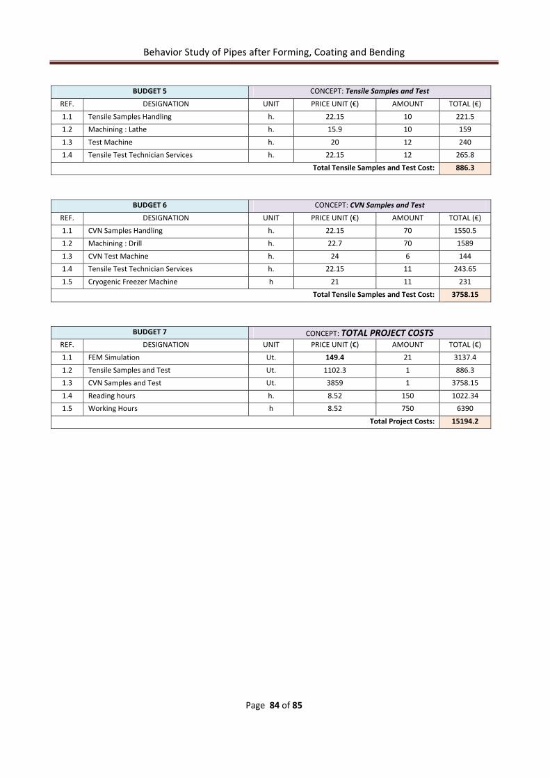
Behavior Study of Pipes after Forming, Coating and Bending
Page 84 of 85
BUDGET 5 CONCEPT: Tensile Samples and Test
REF. DESIGNATION UNIT PRICE UNIT (€) AMOUNT TOTAL (€)
1.1 Tensile Samples Handling h. 22.15 10 221.5
1.2 Machining : Lathe h. 15.9 10 159
1.3 Test Machine h. 20 12 240
1.4 Tensile Test Technician Services h. 22.15 12 265.8
Total Tensile Samples and Test Cost: 886.3
BUDGET 6 CONCEPT: CVN Samples and Test
REF. DESIGNATION UNIT PRICE UNIT (€) AMOUNT TOTAL (€)
1.1 CVN Samples Handling h. 22.15 70 1550.5
1.2 Machining : Drill h. 22.7 70 1589
1.3 CVN Test Machine h. 24 6 144
1.4 Tensile Test Technician Services h. 22.15 11 243.65
1.5 Cryogenic Freezer Machine h 21 11 231
Total Tensile Samples and Test Cost: 3758.15
BUDGET 7 CONCEPT: TOTAL PROJECT COSTS REF. DESIGNATION UNIT PRICE UNIT (€) AMOUNT TOTAL (€)
1.1 FEM Simulation Ut. 149.4 21 3137.4
1.2 Tensile Samples and Test Ut. 1102.3 1 886.3
1.3 CVN Samples and Test Ut. 3859 1 3758.15
1.4 Reading hours h. 8.52 150 1022.34
1.5 Working Hours h 8.52 750 6390
Total Project Costs: 15194.2

Behavior Study of Pipes after Forming, Coating and Bending
Page 85 of 85
9 REFERENCES
[1] ‐ Guo B., Song S., Chacko J., Ghalambor A., Offshore Pipelines, Elsevier (2005).
[2] ‐ Mikael W.Braestrup, Jan Bohl Andersen, Design and Installation of Marine Pipelines, Blackwell Science Editorial 2005.
[3] ‐ Herynk M.D, Kyriakides S., Onoufriou A., Yun H.D., Effects of the UOE/UOC pipe manufacturing processes on pipe collapse pressure, International Journal of Mechanical Science, 533‐553, (2007).
[4] ‐ Braestrup M.W, Andersen J.B, Andersen L.W., Bryndum M., Christensen C.J., Rishoj Nielsen N.J., Design and installation of Marine Pipelines, Blackwell Science (2005).
[5] ‐ Palmer A.C., King R.A, Subsea Pipeline Engineering, Pennwell Editorial 2004.
[6] ‐ American Petroleum Institute, API 5L Specification for Line Pipe, Exploration and Production Department (1995).
[7] ‐ Escoe A.K., Piping and Pipeline Assessment Guide, Elsevier (2006).
[8] ‐ Standard Specification for Epoxy‐Coated Steel Reinforcing Bars, ASTM A 775/A 775M‐97, American Society of Testing and Materials, 1997.
[9] ‐ Montalà F., Materials selection and treatments, EUETIT(2003).
[10] ‐ Dieter G.E., Mechanical Behavior Under Tensile and Compressive Loads, University of Maryland (1986)
[11] ‐ H.E. Davis, G.E. Troxell, and G.F.W. Hauck, The Testing of Engineering Materials, McGraw‐Hill, New York (1964).
[12] ‐ J.M. Gere and S.P. Timoshenko, Mechanics of Materials, 4th ed., PWS Publishing Co., (1997).
[13] ‐ A.A. Griffith, The Phenomena of Rupture and Flow in Solids, Philos. Trans. Soc. (London) A, Vol 221 (1920).
[14] ‐ S.T. Rolfe and J.M. Barsom, Fracture and Fatigue Control in Structures—Applications of Fracture Mechanics, Prentice‐Hall (1977).
[15] ‐ Holman J.P., Heat transfers, CECSA (1999).
[16] ‐ Cengel Y.A., Heat Transfer a practical Approach, Mc. Graw Hill (2003).
[17] ‐ Internal OCAS Project : OE0201020246 Charpy equipment; Number: 41783F2
[18] ‐ J.M. Barsom, Effect of Temperature and Rate of Loading on the Fracture Behavior of Various Steels, Dynamic Fracture Toughness, The Welding Institute (1976).
[19] ‐ Users Abaqus® 6.9.1 Theory Manual, Simulia (2009).
[20] ‐ Source: “ Fabrication of hot induction bends from LSAW large diameter pipes manufactured from TMCP plate”; Microalloyed Steels for the Oil & Gas Industry International Symposium; January 22‐27, 2006
[21] ‐ Source: “First x80 Pipeline section in Italy”; PRCI/EPRG/APIA, Technical Conference May 15‐20, 2005 Orlando‐USA; Europipe.

ABSTRACT
A study of the main types of coatings and its processes that modern industry commonly apply to prevent to the corrosion due to the environmental effects to energetic market pipelines have been done.
Extracting main time and temperature range values, coating heat treatment recreation have been applied to x65 pipelines steel grade samples obtained from a pipe which was formed using UOE forming process.
Experimental tensile tests and Charpy V‐Notch Impact test have been carried out for a deeply knowledge of the influence on the steel once this recreations are applied. The Yield Strength and toughness have been improved despite lower values in rupture strain and ductile‐brittle temperature transition have been obtained.
Finite Element Method have been applied to simulate the entirely pipe cold bending process to predict the mechanical properties and behaviour of the pipe made from x65 steel grade under different conditions.
RESUM
L’estudi dels tipus de recobriments y processos principals que la industria moderna actual aplica per tal de prevenir la corrosió degut als efectes mediambientals sobre les tuberies usades en el sector energètic ha sigut realitzat.
Extraient els principals rangs de valors de temps i temperatura, la recreació dels tractaments tèrmics dels processos de recobriment han sigut aplicats sobre acer de tuberies x65 obtingut d’una tuberia fabricada utilitzant el procés UOE de fabricació.
Tests experimentals de tracció i d’impacte Charpy amb entalla en V han sigut realitzats per tal d’obtenir un profund coneixement de la seva influencia en l’acer un cop aplicats aquests tractaments tèrmics. El límit elàstic i la tenacitat han sigut millorades malgrat valors més baixos de deformació ultima i de temperatura de transició fragil‐dúctil han sigut obtinguts.
Mètodes d’elements Finits han sigut aplicats per tal de simular el procés complet de flexió en fred de tuberies per tal de predir les propietats mecàniques finals així com el comportament de la tuberia feta d’acer x65 sota diferents condicions.