benefit cost model user guide - alberta · alberta transportation benefit cost model - user guide...

Applications Management Consulting Ltd. 2220 Sunlife Place 10123 - 99 Street Edmonton, Alberta T5J 3H1

T 780-425-6741 www.think-applications.com

Benefit Cost Model

User Guide

ATBCMUserGuideV2.PDF

http://www.think-applications.com/

Alberta Transportation Benefit Cost Model - User Guide to ATBenefitCostModelV2.xlsx

Applications Management Consulting Ltd. 2220 Sunlife Place

10123 - 99 Street Edmonton, Alberta T5J 3H1

T 780-425-6741 www.think-

applications.com

Benefit Cost Model User Guide

ATBCMUserGuideV2.PDF

ORIGINAL PREPARED BY: Darryl Howery, Principal, Applications Management Consulting WITH REVISIONS BY: Design Project Management and Training Section, Technical Standards Branch, Alberta Transportation Version 1: April 8, 2015 Version 2: February 3, 2017

ABSTRACT & SUMMATION: This User Guide is a companion document to the Alberta Transportation Benefit Cost Model – ATBenefitCostModelV2.xlsx




Contents Glossary

Section 1: Overview ................................................................................................................... 1

Purpose of the Model ............................................................................................................................................. 1

Analysis Components ............................................................................................................................................. 1

Model Features ....................................................................................................................................................... 1

Limitations of the Model.......................................................................................................................................... 3

Model Components ................................................................................................................................................ 4

Valuation of Analysis Components ......................................................................................................................... 5

Section 2: How to Work with the Model ...................................................................................... 7

Where to Enter Information .................................................................................................................................... 7 Entered Information ............................................................................................................................................................. 7 Cell Protection ..................................................................................................................................................................... 7

Section 3: Completing an Analysis ............................................................................................. 8

Preparing for an Analysis ....................................................................................................................................... 8

Project Definition .................................................................................................................................................... 8 Vehicle Running Costs ‐ Choosing an Approach ................................................................................................................. 8 Project Name ....................................................................................................................................................................... 9 Project Definition ................................................................................................................................................................. 9 Construction Start/End Year ................................................................................................................................................ 9 Vehicle Occupancy & Unit Costs for Time (Default Value Change) ..................................................................................... 9 Vehicle Operating Costs (Default Value Change) ................................................................................................................ 9

Defining Project Alternatives ................................................................................................................................ 10 Project Type ...................................................................................................................................................................... 10 Alternative Name ............................................................................................................................................................... 10 Construction Start/End ...................................................................................................................................................... 10 Historical Capital Investment ............................................................................................................................................. 10 Construction Costs ............................................................................................................................................................ 11 Operating & Maintenance Costs ........................................................................................................................................ 11 Collision Rates by Collision Severity (Default Value Change) ........................................................................................... 12 Applying Collision Modification Factors (CMFs) ................................................................................................................ 12 Collision Costs by Type (Default Value Change) ............................................................................................................... 13 Project Segment Definition ................................................................................................................................................ 13 Project Segment Traffic Mix............................................................................................................................................... 14 Intersection Definition ........................................................................................................................................................ 14 Trip Purpose by Vehicle Type............................................................................................................................................ 15


Emission Costs .................................................................................................................................................................. 15

Project Costs Alt# Tab .......................................................................................................................................... 15

Section 4: How to Interpret the Results of an Analysis ............................................................. 16

Project Cost Summary.......................................................................................................................................... 16 Project Cost Graphs .......................................................................................................................................................... 16

Results .................................................................................................................................................................. 17

Summary .............................................................................................................................................................. 18 Internal Rate of Return ...................................................................................................................................................... 18 Break Even Point ............................................................................................................................................................... 19 Discounted Total Cumulative Costs (in Present Values) ................................................................................................... 19 Discounted Investment Costs (in Present Values) ............................................................................................................. 19 Discounted Benefits [Non‐Investment Cost Savings] (in Present Values) ......................................................................... 20 Benefit/Cost Ratio .............................................................................................................................................................. 21

Section 5: How to Update the Model ........................................................................................ 22

Administrator and User Updates .......................................................................................................................... 22

Model Components .............................................................................................................................................. 22 Base Year .......................................................................................................................................................................... 22 Analysis Definition Factors ................................................................................................................................................ 22 Project Type Categories .................................................................................................................................................... 23 Construction Cost Categories ............................................................................................................................................ 23 Operating & Maintenance Cost Categories (Specified Maintenance) ................................................................................ 23

Maintenance Cost Categories by Surface Type (Scheduled Maintenance) ....................................................................... 24 Vehicle Default Values ...................................................................................................................................................... 24 Road User Gradient Factor Categories (Texas [Curvature & Gradient] Vehicle Operating Costs) .................................... 27 Collisions ........................................................................................................................................................................... 27 Emission Costs by Type .................................................................................................................................................... 29

Appendix 1: Summary of Model Variables

Appendix 2: Alberta Traffic Collision Data


Glossary (Ordered alphabetically)

Note: the previous Alberta Transportation and Utilities (ATU) Benefit Cost Model published in 1991 is available as a separate document on the Department’s website.

Benefit Cost Analysis1

Benefit cost analysis is the exercise of evaluating a planned action by determining what new value it will have. Benefit cost analysis finds, quantifies, and adds all the positive factors. These are the benefits. Then it identifies, quantifies, and subtracts all the negatives, i.e. the costs. The difference between the two indicates whether the planned action is advisable. The key to doing a successful cost-benefit analysis is making sure to include all the costs and all the benefits and properly quantify them. Where the benefits of a project exceed costs, it can be determined it would be beneficial to undertake the project. Where more than one project is considered, the alternative where benefits exceed costs the most would be the preferred project.2

Benefit Cost Ratio3

Typically the results of a benefit/cost analysis are summarized in a Benefit/Cost Ratio (BCR). This calculation compares a stream of cost savings (benefits) over time compared to the costs, or investment in the project. The benefit cost ratio is the present value of benefits divided by the present value of costs. The benefits (in the numerator) associated with each Alternative are equal to the non-investment cost savings for that Alternative as compared to the ’do minimum’ alternative (Alternative 1). Costs are reflected in the denominator, and are obtained by comparing the Total Discounted Investment Costs of each alternative to the Total Discounted Investment Costs for Alternative 1. Where the BCR is greater than 1, benefits exceed costs and the project provides overall benefits. This measure however, does not consider the scale of expenditures. For example, a small project may produce a greater BCR but have a smaller overall benefit.4. Note: Since everything is compared against it, Alternative 1 will not have a BCR because the benefits (cost savings) cannot be calculated. Benefits

The Discounted Benefits are calculated by taking all the Non-Investment Costs for the Alternative considered and subtracting the Non-Investment Costs estimated for the ‘do minimum’ option (Alternative 1). As a result, Benefits associated with Alternative 1 are nil. These benefits have been used as the numerator in the BCR calculation.

Break Even Point5

The Break Even Point, also known as the payback period, refers to the period in time when funds expended in an investment are recuperated, i.e. the project has “paid for itself.” If the project alternative always has a higher net cost (including any cost savings in road user costs), there is no break-even point in the analysis timeframe.

1 Appendix 3: Benefit Cost Analysis Guide, ATU (1991) page 1 2 http://www.inc.com/encyclopedia/cost-benefit-analysis.html 3 Appendix 3: Benefit Cost Analysis Guide, ATU (1991) page 31 4 Appendix 3: Benefit Cost Analysis Guide, Treasury Board of Canada Secretariat, 2007, page 27 5 Appendix 3: Benefit Cost Analysis Guide, ATU (1991) page 20

i

http://www.inc.com/encyclopedia/cost-benefit-analysis.html

Alberta Transportation Benefit Cost Model - User Guide to ATBenefitCostModelV2.xlsx Discount Rate6

The discount rate is the real rate of interest (nominal rate of interest minus inflation). It is also described as the real cost of long-term borrowing, as the purchasing power of money normally decreases over any given period of time due to inflation and uncertainty. A discount rate adjusts the value of money for time, expressing expected future monetary quantities in terms of their worth today. The Discount Rate used in Alberta Transportation analyses is selected by the department as it is a choice made by the client as a matter of policy. Currently Alberta Transportation’s Discount Rate is set at 4%. Other agencies may use different Discount Rates for various reasons however the practices of other agencies do not affect the Alberta rate. The costs are discounted because money has a time value, known as an opportunity cost, which means that money invested today could earn interest elsewhere. To compensate, future payments need to be higher so that they equal today's dollars. Additionally, time value accounts for the cost of capital, the cost for a company to borrow investment money, over time, at a specific interest rate. In the model, Total Discounted Costs indicate the value of a project as a cumulative total of both costs and cost savings over a project’s life in today's dollar terms The more savings an alternative produces, the lower the total cost.

Internal Rate of Return (IRR)7

The Internal Rate of Return is the rate of discount that makes the present value of the benefits minus the costs over time equal to zero8. Specifically, the IRR considers the difference in costs and cost savings between an Alternative and the ‘do minimum’ option over the project’s life. When there are no cost savings associated with that Alternative compared to the ‘do minimum’ for a particular year, the resulting value will be negative; in this case, an error message will appear as the IRR function in excel cannot perform on a set of all negative numbers. Where the IRR is greater than the discount rate, the benefits of the project are greater than the expected or required return on the investment.9

Note: - There will never be an IRR value for the ‘do minimum’ option as it is not being compared to anything. - The standard time frame used for the IRR is 20 years.10

Investment Costs (in Present Values)

Investment Costs are defined as Construction Costs plus any Rehabilitation costs that are invested in the project over the forecast period, discounted to their present values.11 To calculate a BCR, benefits (cost savings from one alternative to another) need to be compared to an investment.

Undiscounted Cost Comparison

This is the comparison of the total undiscounted costs between the selected Alternative and Alternative 1 for each year.

6 Appendix 3: Benefit Cost Analysis Guide, ATU (1991) page 21 7 Appendix 3: Benefit Cost Analysis Guide, ATU (1991) page 31 8 Appendix 3: Benefit Cost Analysis Guide, Treasury Board of Canada Secretariat, 2007, page 27 9 The Principles of Practical Cost-Benefit Analysis, Sugden, R & Williams, A, Oxford University Press 1978, page 20. 10 Twenty years is a reasonable timeframe over which a public investment can be expected to provide a positive payback. 11 This differs from the Discounted Total Costs in that they include all costs.

ii

Alberta Transportation Benefit Cost Model - User Guide to ATBenefitCostModelV2.xlsx Net Present Value (NPV)

The NPV calculation consists of two financial concepts that evaluate a set of costs and benefits over time: The “net” is the difference between all costs and all benefits (savings in user costs), discounted to present

values. The present value takes into account the time value of money; this adjusts to expenditures and cost

savings, as they occur over time, so they can be evaluated equally Note: Since Alternative 1 does not have any calculated benefits (as described above) it will not produce a value for NPV. Sunk Costs 12

Sunk costs, or expenditures that have occurred in the past and are therefore not recoverable, are not relevant for consideration in benefit-cost analysis. Benefit cost analysis is forward looking with the aim of providing information about future investment decisions.

Total Cumulative Costs (in Present Values)13

The cumulative total of all costs and benefits (in the form of cost savings) of one alternative over the project’s life, discounted to today’s dollars.

12 Appendix 3: Benefit Cost Analysis Guide, ATU (1991) page 20 13 Appendix 3: Benefit Cost Analysis Guide, ATU (1991) page 30

iii

Alberta Transportation Benefit Cost Model - User Guide to ATBCmodelV2.xlsx

Section 1: Overview Purpose of the Model

Benefit cost analysis is an analytical tool that provides information about the economic merits of a proposed investment or alternative investment options. With regards to transportation project evaluation, benefit cost analysis measures the changes in benefits and costs over time arising from an investment in one of several alternatives, as compared to a “do minimum” option.

A benefit cost analysis determines whether a proposed project is economically desirable (when benefits exceed costs). Benefit cost analysis can also be used with other information to select which project among competing project alternatives should be funded given a budget constraint, and to compare the effects of projects that may accomplish different objectives.

The purpose of the Alberta Transportation Benefit Cost Model is to determine which road or bridge project, given a number of project alternatives, provides the best return on investment. NOTE: All costs are inputted into the model at their present estimated value, meaning the effects of inflation are ignored for all costs.

Analysis Components

The Alberta Transportation Benefit Cost Model evaluates the impact of various project alternatives in each of the following areas:

Initial Construction Project Costs (Investment)

Maintenance and Operating Costs

Rehabilitation Costs (capital costs required to maintain the asset at a specified condition)

Road User Costs: Vehicle operating costs – see model features for two different calculation approaches.

Important: It is recommended the California (Fuel & Non-Fuel) approach be used for all projects unless the curvature or gradient varies significantly between alternatives, in which case the Texas (Curvature & Gradient) approach would be used.

Travel time costs Collision costs, and

Environmental costs associated with vehicle emissions.

Other Costs It is noted that other cost types may be relevant for some projects. For example, there may be costs associated with the protection of environmental assets, or costs associated with the mitigation of potential negative environmental impacts of a project. These costs can be defined in user defined categories as either a capital cost or an on-going operating cost, whichever is most appropriate.

Model Features

The Alberta Transportation Benefit Cost Model includes a number of features that allow for flexibility in evaluating different types of projects under different circumstances. The key features of the model include the following:

1


Up to eighty (80) year timeframe for the analysis.14

Analysis of up to three Alternatives (including a ‘do minimum’ alternative). These Alternatives refer to different or alternative projects that could be undertaken, which are usually compared to a ‘do minimum’ alternative. The ‘do minimum’ alternative (Alternative 1 in the model) involves the least work; even if one option is to leave the asset in its current condition, there would still be some costs associated with maintaining the asset. Other alternatives should represent reasonable options to the ‘do minimum’ alternative that are technically feasible, but likely to have different costs and potential cost savings. While three alternatives will likely suffice for most instances, if additional alternatives need to be considered, it is recommended to duplicate the model file with the Alternative 1 data contained in the file. Two additional alternatives to the ‘do minimum’ (Alternative 1) can be specified in the new duplicate model file.

Sensitivity analysis of each Alternative: variations on the Alternatives with some parameters that can be modified using a percentage adjustment. The following external factors can be modified: the discount rate, capital costs, operating and maintenance costs, road user costs (vehicle operating costs, travel time costs and collision costs) and emission costs.

Flexible project definition categories: The user can define up to 10 different types of projects for analysis.

Flexible construction cost categories: The user can define up to 8 different types of project construction cost categories. This will allow for the definition (and separation) of costs that might be specific or unique to a project, such as environmental impact mitigation costs.

Flexible construction period: The construction period is defined for each Alternative.

Flexible operating and maintenance cost categories: The user can define up to 5 operating and maintenance cost categories.

Flexible vehicle definition categories: The user can define up to 10 different types of vehicles.

Vehicle Operating Costs, which can be calculated in one of two ways:

Important: It is recommended the California (Fuel & Non-Fuel) approach be used for all projects unless the curvature or gradient varies significantly between alternatives.

1. California (Fuel/Non-Fuel Option): Utilizes average fuel and non-fuel vehicle operating costs by vehicle type similar to the CalTrans model. This approach should be used where horizontal and vertical geometry is not a factor (does not vary significantly) between alternatives. The vehicle operating costs for the California option are currently based on a value of $0.505/km/passenger. This is the current calibration to suit Alberta conditions. The calibration may be changed by the Administrator if warranted based on changing conditions. In the user guide and model, this option will be referred to as California (Fuel & Non-Fuel) approach.

2. Texas (Curvature & Gradient Option): This option utilizes curvature and gradient cost factors that were originally estimated by the Texas Research Development Foundation for the Federal Highway Administration (1982 US). These costs were adjusted for inflation to reflect the Alberta context in 1989.15 This option should be used when the curvature and gradient of some or all of the alternatives vary significantly. In the user guide and model, this option will be referred to as Texas (Curvature & Gradient) approach.

14 The analysis results can be viewed for any time period, up to 80 years, including the construction period. For example, if the construction period is 5 years, the operation of the project would be projected for a total of 75 years. The results for any individual year in the forecast period can be viewed in the ‘Results’ tab of the model. 15 Benefit Cost Analysis - Vehicle Running Costs, Alberta Transportation & Utilities, Traffic Engineering Branch, January 1989.

2


Vehicle Operating Cost and Collision default values can be redefined for specific projects where the default values are not appropriate.

Benefit Cost Analysis Results: The model uses the following standard Benefit Cost Analysis indicators to measure the relative desirability of each alternative. For an explanation of terms, refer to the Glossary.

Benefit Cost Ratio Benefits [Non-Investment Cost Savings] (in Present Values) Break Even Point (Payback Period) Internal Rate of Return (IRR) Investment Costs (in Present Values) Total Discounted Costs (in Present Values) Net Present Value: NPV is the difference between the benefits and costs, discounted to present values

Limitations of the Model The Benefit Cost Model has the following known limitations that should be understood by the analyst.

As with all models, the quality of the analysis and results will depend on the quality of the information used to conduct the analysis.

The model is limited to evaluating individual projects and not the infrastructure system.

There are limited benefit cost analysis indicators for Alternative 1 (‘do minimum’ alternative) as most indicators require the estimation of benefits. The benefit cost analysis indicators available for Alternative 1 are: Discounted Total Cumulative Costs; and Discounted Investment Costs. Example situation: a low volume road that meets the requirement for grade widening. In this case the “do minimum” (Alternative 1) is the minimum that the department can tolerate, which would be “no widening”. Depending on the project, this may result in a narrower shoulder or narrower lane but likely no reduction in road user costs unless the posted speed has to be reduced. The alternative under consideration (grade-widening) would have considerable cost and very little benefit as road user costs would not be reduced very much except due to the addition of shoulder rumble strips and possibly flatter side slopes. Consequently, the return on investment would likely be very low due mostly to the low volume nature of the project. Furthermore, if there is an absence of collision history, no quantifiable benefits would be produced in the form of collision cost savings. The ‘do minimum’ option may produce the most desirable numbers in the model even though an improvement may be warranted for safety reasons. Engineering judgment should be exercised in such situations. The department is willing to look at departures from normal practices on low volume roads. This should be undertaken as a Design / Practice Exception or documented as a “Project Requirement” in advance by AT.

The 80 year time frame for analysis may be limiting for some cases, e.g. the expected life of a bridge is typically 100 years.16 However, any benefits or costs expected beyond year 80 may be discounted back to 80 years and entered for that year (year 80). For example, for year 81 all benefits or costs would be multiplied by F81:

Benefits or Costs Year 81

F81 = ------------------------------------------------------ (1 + discount rate)81-80

16 As the length of the analysis increases, the discounted value of these future values becomes increasingly smaller. For example, the discounted value of a $100 investment 50 years in the future discounted at an annual rate of 4% is equal to $7.85.

3


Model Components The Alberta Transportation Benefit Cost Model has four main components as follows:

Model Parameters: This section of the model consists of 9 tabs as follows:

Parameters: This tab contains default information, including Sensitivity Analysis Adjustments, Project Type Categories, and various Cost Categories. Some of these variables can be altered for specific analyses (in the Project Definition tab) where the default values are not appropriate. This tab does not need to be updated for each analysis, but should be reviewed periodically. The user should also understand what default values are being utilized for their project. If the default values are inappropriate, it is up to the user to modify them accordingly.

Maintenance: This tab provides the Maintenance costs for each of the three Scheduled Maintenance categories and calculates the associated costs for each segment of the project alternative. NOTE: This is different from Specified Maintenance costs, which are user-defined maintenance costs and can be used on their own or in addition to Scheduled Maintenance costs.

RUC Alt# (3 tabs): This tab calculates the road user costs (per day) associated with vehicle running costs, travel time costs and emission costs. These costs are estimated by vehicle type for each segment of the project defined by the user in the ‘Project Definition’ area. A separate tab exists for each Alternative (up to three alternatives can be defined by the analyst).17

Collision Rates: This tab provides the rate of collisions (per 100 million vehicle kms) by varying AADT for different road types. NOTE: If the user has project-specific information available, these should be used first. If not, then the user has the option of using the information from the charts in this tab, which must be input manually into ‘Project Specific Values,’ or using the default values if the applicable rates are not available. Collision Rates adjusted with Collision Modification Factors (CMFs) must be entered as Project Specific Values also in the individual Alt# tabs.

Emissions: This tab provides the rate of emissions (gms/km) by the speed of vehicle for each vehicle type and for each emission type defined by the user in Parameters. NOTE: If new vehicle types are added, the emissions tab (gms/km) will need to be updated to reflect the new categories defined by the user.

Fuel Consumption: The California (Fuel & Non-Fuel) approach to estimating running costs (vehicle operating costs) by fuel and non-fuel costs per km takes into account an estimate of fuel consumption by speed and vehicle type. This tab provides a cost factor from the average cost defined in Parameters.18 The fuel consumption per vehicle type is estimated based on current information published in the California model. This is one of the items taken into account in the calibration of the model to an Alberta value.

Project Definition: This section of the model consists of 7 tabs as follows:

Project Definition (Defn): This tab contains information specific to the project being analyzed. This includes the labels that will be used for the model, the definition of the project type and possible changes to default values that have been set in the Parameters tab.

17 Note that the Texas (Curvature & Gradient) approach to estimating Road User Costs using definitions and values of gradient and curvature for different road surfaces (pavement/gravel) and vehicle type have not been updated to reflect changes in fleet composition in this model. Figures from the Texas (Curvature & Gradient) analysis have been adjusted to reflect change in inflation over the period from when the original figures were produced (1989) to 2013. 18 This factor is built into the model and is set by the Department.

4

Alberta Transportation Benefit Cost Model - User Guide to ATBCmodelV2.xlsx Alt# (3 tabs): This tab contains information specific to the alternative being analyzed. This tab requires

inputs about each Alternative that will be considered in the analysis. Alternative 1 is the option against which other Alternatives are evaluated, and therefore it should be defined as the ‘do minimum’ option.

TrafficAlt# (3 tabs): This tab calculates the traffic projected for each Alternative and applies this forecast to the unit costs for vehicle operations, travel time, emissions and collisions. It does not require any inputs.

Analysis Results: This section of the model provides a summary of the costs calculated for the analysis, and the benefit-cost analysis results.

Project Costs # (3 tabs): This tab summarizes the costs associated with each Alternative defined by the user over the 80 year analysis timeframe. IMPORTANT: rehabilitation costs must be manually entered by the user into the rehab costs column for each year at their present estimated values.

Results: This tab calculates the detailed benefit-cost analysis results for each year and each of the Alternatives defined by the user.

Summary: This tab provides a summary of the benefit-cost analysis results for each of the Alternatives defined by the user.

Analysis Support Data: A number of worksheets (located in a separate file) have been used to calculate data input to the model. The user does not have access to these worksheets. These worksheets will be modified by the Department if warranted. These include:

Emissions Conversion Table: This table takes the CalTrans Benefit Cost19 model’s vehicle emissions estimates (as input by the user) and converts the imperial measures for speed and volume to metric. This data is imported into the Emissions tab in the model.

Value Updates Table: This spreadsheet uses historical cost indexes to update various values used in the model.

Valuation of Analysis Components At the core of any benefit cost analysis is the valuation of incremental changes in expenditures or revenues that may be associated with a project or its alternatives. How these expenditures or revenues are evaluated and incorporated in the analysis is a critical consideration. Real Dollars This benefit cost model deals with all values expressed in real base year dollars which do not include inflation; i.e. their present estimated values. As a result, all base values and expenditure data used in the model will need to be expressed in these terms. Where expenditures include inflation or are expressed in real values for another year, other than the base year, these values will need to be converted to the base year dollars (present estimated value) using an appropriate factor. Real Discount Rate As this benefit cost model does not include inflation, the discount rate used to account for the time value of money, and bring all future dollar values back to the base year, must be a ‘real’ discount rate.20 The default value used in the model is 4% per annum, as per AT’s typical practice.

19 California Life-Cycle Benefit/Cost Analysis Model (Cal-B/C). February 2009. 20 Appendix C: Benefit Cost Analysis Guide ATU (1991), page 22

5

Alberta Transportation Benefit Cost Model - User Guide to ATBCmodelV2.xlsx Perspective The components of a benefit cost analysis and the valuation of these components depends upon the perspective, or point of view defined for the analysis. For this benefit-cost model, the perspective is the social point of view for the Province of Alberta. This social perspective should consider all relevant expenditures and costs for society’s point of view, limited to Alberta. Inputted Values - Shadow Prices21 In some instances the market does not provide values for some components that are relevant for this analysis. In other cases, the market value may not reflect the ‘social’ value of these components from the perspective discussed above. As a result, where this is relevant, there may need to be adjustments to the values used in the analysis. In other instances, where these values are not available from market information, inputted values or shadow prices should be considered. For example, the travel time associated with passengers has no ‘market’ value. However, studies have been conducted into the ‘social’ value of travel time for passengers. The most relevant of these estimates should be used in the analysis to quantify this component. The most significant examples of factors that are currently used in the model include the costs for passenger travel time and emission costs. The model provides ‘default values’ that may be over-written by the user where warranted. Direct Expenditures and Costs22 The undertaking of new economic activities, such as construction, not only contribute to the growth in the economy through the funds spent on the project, but also create the potential for additional expenditures on indirect and induced economic activities. These additional indirect and induced expenditures are associated with upstream purchases of goods and supplies required to support the project and the subsequent income effects generated by the project. In this benefit cost model, only the direct expenditures and costs have been included in the analysis. Transfers23 Some types of revenues and expenditures, from a social perspective, do not represent real change, but are rather transfers from one group of economic agents in the economy to others. This typically includes subsidies, grants and taxes, all which are transfers from taxpayers to other groups in the economy. Transferring benefits or costs from one economic agent to another has no effect on economic efficiency.

21 Appendix C: Benefit Cost Analysis Guide ATU (1991), page 13 22 Appendix C: Benefit Cost Analysis Guide ATU (1991), page 12 23 Appendix C: Benefit Cost Analysis Guide ATU (1991), page 18

6


Section 2: How to Work with the Model Where to Enter Information

The model has been designed so that all user inputs are entered in cells with the following formatting:

In some instances, a drop down menu has been built into the model with pre-defined selections for the user to choose from. To get the drop down menu, click in the cell and the selection options will become visible.

The model has pre-selected Vehicle Running Costs to be calculated by the California (Fuel & Non-Fuel) method. When selection of the Texas model is warranted, the user may select it from the drop-down menu. If changed, the selected method will be shown after the user hits ‘return’.

Reminder: It is recommended the California (Fuel & Non-Fuel) approach be used for all projects unless the curvature or gradient varies significantly between alternatives, in which case the Texas (Curvature & Gradient) approach would be used.

Entered Information

Information that has been entered in the model and used elsewhere in the model is displayed as orange text in either a white or grey background as follows:

In this example, each of the vehicle types (e.g. Passenger, RV, etc.) have been entered by the user elsewhere in the model (Parameters tab) and are shown here in orange text. Similarly, the Default Values for Occupancy, Work/Bus $/hr and Other $/hr were entered in the Parameters tab. In many cases, the default specified values may be modified when data is available at a project level. However, the changes to default values should only be made in the user input cells. This process is outlined in more detail below.

Cell Protection All cells that do not require an input from the user have been 'locked' and 'protected'. This will ensure that these cells are not accidentally altered. Altering cells that do not require information from the user may affect the integrity of the calculations in the model.

7


Section 3: Completing an Analysis

Preparing for an Analysis Before working with the model, it may be valuable to review the required information so it can be collected and/or generated prior to starting the analysis. Every analysis will require the development of information for a ‘do minimum’ (Alternative 1) option and at least one (up to two) Alternative options. The same information will be required for each of these Alternatives.

NOTE: It is important that Alternative 1 be defined as the ‘do minimum’ alternative for the calculation of the economic indicators as shown in the Summary tab. This is because the determination of some of the economic indicators is based on a comparison of values associated with each alternative against those of Alternative 1.

Project Definition The Project Definition tab includes the definition of variables that will affect the evaluation of the project as a whole. The Alternatives to be analyzed are defined in the Alt # tabs.

Vehicle Running Costs ‐ Choosing an Approach The model contains two approaches to estimate vehicle running costs. The California (Fuel & Non-Fuel) approach, which is the default approach, is centered on the CalTrans model and is based on distance-related fuel and non-fuel costs. The California (Fuel & Non-Fuel) vehicle running costs are estimated using fuel and non-fuel vehicle operating costs for each vehicle type based on the segment length and running speed, not considering the effect of gradient or curvature specified in the model.

The Texas (Curvature & Gradient) approach relies on the definition of segment curvature and gradient for each segment of the project, and the unit costs by vehicle type associated with the gradients and curvature. It is recommended that the Texas approach only be used if the curvature or gradient varies significantly between alternatives. The factors used in the Texas (Curvature & Gradient) approach originated in part from data compiled by the Texas Research and Development Foundation in 1982 for the Federal Highway Administration. For the original Alberta Transportation Benefit Cost Model (published in 1991), these numbers were converted to 1988 Canadian dollars using Alberta consumer prices for items such as fuel, oil, tires, depreciation, etc. These were then updated from 1988 to 2012 based on the Transportation Price Index. These 2012 factors are used in the new version of the model.24

Either approach can be used to estimate vehicle running costs. When gradient and/or curvature improvements are an important feature of an alternative being evaluated, it is recommended that the Texas (Curvature & Gradient) approach be used. Sensitivity analysis can be conducted using either the Texas (Curvature & Gradient) or California (Fuel & Non-Fuel) approaches to see how the benefit-cost results vary with each approach.

The desired approach to estimating road user costs can be implemented by clicking on the cell to the right of Road User Cost and selecting either California (Fuel & Non-Fuel), which the model is set to by default, or Texas (Curvature & Gradient).

24 Benefit Cost Analysis - Vehicle Running Costs, Alberta Transportation & Utilities, Traffic Engineering Branch, January 1989.

8

Alberta Transportation Benefit Cost Model - User Guide to ATBCmodelV2.xlsx Reminder: It is recommended the California (Fuel & Non-Fuel) approach be used for all projects unless the curvature or gradient varies significantly between alternatives, in which case the Texas (Curvature & Gradient) approach would be used.

Project Name

The project being evaluated should be labeled by entering a Project Name.

Project Definition

This table provides an overview of the Alternatives’ names. Up to three alternatives can be defined for each project being evaluated. The names are defined in the Alt # tab(s).

Construction Start/End Year

This table provides an overview of the construction start and end dates, and when the project would begin operations. The timing of construction is defined in the Alt # tab(s).

Vehicle Occupancy & Unit Costs for Time (Default Value Change)

The default values for vehicle occupancy and the unit costs (from the Parameters tab) can be modified for the project by entering the desired value in the ‘Project Specific Values’ field. This updated value is then reflected in the ‘Values Used in the Model’ portion of the table.

Vehicle Operating Costs (Default Value Change)

The default values for vehicle operating costs used for the California (Fuel & Non-Fuel) approach to estimating vehicle running costs (from the Parameters tab) can be modified for the project by entering the desired value in the ‘Project Specific Values’ field. This updated value is then reflected in the ‘Values Used in the Model’ portion of the table.

9


Defining Project Alternatives

The Alternatives to be evaluated are defined in the Alt # tab (i.e. Alt 1, Alt 2, Alt 3). To conduct an analysis, at least 2 Alternatives must be defined. It is strongly recommended that Alt 1 be the ‘Do Minimum’ alternative against which other alternatives (that involve more work) are evaluated.

Project Type

Select an option from the list of project type categories. The project type has default values for running speed and project life associated with it (see Parameters tab). It is particularly important to select a Project Type for Intersection – New or Upgrade when applicable so that the model applies the correct time delay costs. The project should also be given a locale - either rural or urban.

The project type categories can be modified in the Parameters tab. The process for modifying the project type categories is described in Section 5: Project Type. Alternative Name

Enter a name that reflects an identifiable characteristic of the Alternative.

Construction Start/End

Define the years over which construction of the Alternative will take place. The year following the end of the construction period is assumed to be the first year of operation.

Historical Capital Investment

Defining the original (historical) cost of the project is required only when no significant construction costs are needed for the alternative being examined. It is intended to only be used as an informational value and will not affect the end results. If a reasonably accurate historical capital investment value is not available, this cell may be left blank. In benefit cost analysis terms, any costs incurred prior to the analysis are considered to be ‘sunk costs’ and not relevant to the future investment decision making.

10


Construction Costs

The construction cost categories (defined in the Parameters tab) and construction period will define the cells that are available to enter the associated construction costs (orange cells). The total cost by category is provided in each column and total cost by year in each row.

Operating & Maintenance Costs

There are two approaches to determining the operating and maintenance costs: Specified Operating and Maintenance costs that are defined by the user; and Scheduled Maintenance Costs that are from Alberta Transportation’s RODA model. It is possible to use either of these options, or a combination of the two.

The user Specified operating and maintenance cost categories are used to enter the associated costs (orange cells); the costs are annual for the entire roadway project. The total operating and maintenance costs for the first year of operation are totaled in the year 1 row. Should the user wish to not use one or all of these categories, a zero can be entered in the relevant cell(s). The cost will increase proportionately with the traffic growth rate defined by the user in the project segment definition section.

IMPORTANT: If any Specified operating and maintenance costs are entered, they will be added to Scheduled operating and maintenance costs identified by segment as discussed below. If the user wishes to only use Scheduled operating and maintenance costs, a zero should be entered in each of the Specified operating and maintenance cost categories. If the user wishes to add to or adjust the Scheduled operating maintenance costs, the adjusted amounts should be entered in the Specified operating and maintenance cost categories.

The Scheduled operating and maintenance costs are defined by segment in the ‘Project Segment Definition’ table. The Scheduled operating and maintenance costs are unique to each segment in the project and must be specified for each segment to be used in the analysis. See Maintenance Cost Categories by Surface Type (Scheduled Maintenance) below.

11

Alberta Transportation Benefit Cost Model - User Guide to ATBCmodelV2.xlsx IMPORTANT: If the user wishes to only use Specified operating and maintenance costs, costs should be specified as described above and ‘Do Not Use’ should be selected for each Project Segment in the Maintenance Cost Category column of the ‘Project Segment Definition’ table (Scheduled Maintenance). Collision Rates by Collision Severity (Default Value Change) The default values for the collision rate and distribution of collisions by collision severity (from the Parameters tab) can be modified for the Alternative by entering the desired value in the ‘Project Specific Values’ field. This updated value is then reflected in the modified ‘Values Used in the Model’ portion of the table. It would be most appropriate to use actual collision rates if they are available for the project area. If these are not available, collision rates from 2012 for various road types at varying levels of AADT can be obtained from the charts in Appendix 2 or in the Collision Rates tab in the model, and may be entered as ‘Project Specific Values’. Lastly, if the charts do not contain data that applies to the situation, the default values should be used.

Applying Collision Modification Factors (CMFs)

When comparing alternatives, there is generally an improvement completed from one to the other which may result in a change in the expected collision rate. A crash modification factor is a multiplicative factor used to compute the expected number of collisions after implementing a given countermeasure at a specific site. The Crash Modification Factors Clearinghouse25 is a web-based database of CMFs along with supporting documentation to help transportation engineers evaluate the most appropriate countermeasure for their safety needs. Some improvements (such as roundabouts) may reduce the collision severity significantly while leaving the number of collisions unchanged or perhaps increased. The analyst needs to take into account both the collision rate and collision severity associated with any proposed improvements compared to the ‘do minimum’ alternative (Alt 1). After the new collision rate is calculated by applying a CMF, it can be entered as a Project Specific Value as shown in the screenshot below. E.g. Applying a CMF of 0.8 (an expected 20% decrease in collisions) to the default 2 Lane paved road collision rate of 117.33 would result in a Project Specific Value of 93.9. The analyst should use project specific collision history information where available and applicable rather than the default values for the network.

25 Crash Modification Factors Clearinghouse. U.S. Department of Transportation, Federal Highway Administration. www.cmfclearinghouse.org 12

Alberta Transportation Benefit Cost Model - User Guide to ATBCmodelV2.xlsx Collision Costs by Type (Default Value Change)

The default values for the cost of collisions by type of collision (from the Parameters tab) can be modified for the project by entering the desired value in the ‘Project Specific Values’ field as shown in the screenshot below. This updated value is then reflected in the modified ‘Values Used in the Model’ portion of the table.26

Project Segment Definition

The project segment definition is required to calculate various components of road user costs. The inputs on this table support both the California (Fuel & Non-Fuel) and Texas (Curvature & Gradient) approaches to estimating vehicle running costs, as well as other road user cost components including generating a forecast of traffic volumes for an alternative.

Before entering data into this table, depending on the complexity of the project being analyzed, it may be necessary to plan how the inputs are best defined. While there are 20 possible segments that can be defined for the project, for very complex projects, it may be necessary to combine components that have common features, such as gradient and curvature. Where components of a project are combined it will be important to also combine other relevant information, such as length and traffic volume. Another important consideration is to combine only components of a project into segments that share common features, such as surface type or traffic direction.

The individual data items contained in this table include:

Segment Name: Enter a unique identifying name for each segment of the project.

Length: Enter the length of the segment in km.

Surface Type: Select either Paved or Gravel.27

Road Type: Select one of: 2 lane, 4-lane undivided, 4-lane divided expressway or 4-lane divided freeway.28

Gradient (Texas [Curvature & Gradient] Vehicle Running Costs Only): Enter a grade that best reflects the average for the segment (an integer between -8 to +8).

Traffic Direction (Texas [Curvature & Gradient] Vehicle Running Costs Only): Select either 1 Way or 2 Way.29

Curvature Radius (Texas [Curvature & Gradient] Vehicle Running Costs Only): Enter the value that best reflects the average for the segment.

26 Note that the threshold for reporting Property Damage Only (PDO) collisions increased from $1,000 to $2,000 on January 1, 2011. 27 Different gradient unit costs for the Texas (Curvature & Gradient) approach to estimating vehicle running costs as well as collision costs for both California and Texas approaches. 28 Allows for differentiation of maintenance costs and collision rates by Road Type. 29 In determining gradient costs, 1 Way assumes all traffic goes in the direction of the assigned gradient. 2 Way assumes traffic is evenly split.

13


Curvature Superelevation (Texas [Curvature & Gradient] Vehicle Running Costs Only): Enter the value that best reflects the average for the segment.

Traffic Growth Driver: Select either Linear or Exponential.

Traffic Growth Rate: Enter a growth rate for traffic on the selected segment.

Average Running Speed: Enter the average vehicle speed on the selected segment.

Maintenance Cost Category (Scheduled Maintenance): Select the appropriate road maintenance cost category for the selected segment (e.g. Gravel, Paved Base, Paved 2nd). These maintenance cost categories were set up using information from Alberta Transportation’s RODA model. If it is more appropriate to define specific road maintenance costs for this project, use the Operating & Maintenance Cost definitions defined in the Parameters tab and specify the appropriate costs for the option in the Alt # tab. When using this option, select ‘Do Not Use’ for each road segment Maintenance Cost Category.

Age of Surface: When using the road maintenance costs from the RODA model, it is necessary to specify the age of the surface. Enter the age of the surface for each segment of the Alternative.

Project Segment Traffic Mix

The mix of traffic by Vehicle Type must be allocated for each segment. The Traffic Mix must add up to 100% for each segment; if it does not, an error message will appear.

Intersection Definition

When comparing intersection improvements, the user can enter estimated delay times (from capacity analysis software) in seconds per vehicle for AM Peak, PM Peak, and Off-Peak averages (both daytime and nighttime). Volumes on each approach should also be entered. These volumes and delays are converted into time loss costs based on the time values for money embedded in the model. The time loss costs are reflected in the TrafficAlt# tabs for each alternative.

This is applicable to Project Types of “Intersection – New” or “Intersection – Upgrade” only. When these project types are chosen, the time cost of travel will not be accounted into the road user costs – rather the time loss costs will instead.

NOTE: This method assumes that the growth rate of the delay is equal to the traffic growth rate. Therefore, the user should ensure that the traffic growth rate is selected correctly under project segment definition. The model uses the traffic growth driver and rate, as well as AADT, as indicated for Segment 1.

14


Trip Purpose by Vehicle Type

The share of traffic by trip purpose (work/business or other) must be set for each Vehicle Type. When the share of trips that are ‘Work/Business’ are entered for a Vehicle Type, the share of ‘Other’ trips is calculated by the model.

Emission Costs

Emission costs are estimated based on the fuel consumption as per the number of vehicle kilometres travelled by each vehicle type and running speed on each segment of the defined project. These calculations are based on data from the California Life-Cycle Benefit/Cost Analysis Model, including the emission values.30 The calculation of emission costs depends on data entered and estimated in the model for other variables and as a result, there is no additional data required to complete these calculations. A ‘factor’ has been incorporated in the model that can be used to adjust all the emission calculations up or down so they may better reflect Alberta values. This factor is located in cell CN8 of each of the ‘Traffic Alt#’ tabs of the model.31 A value of 1 uses the values provided in the Cal-B/C model. The user does not have access to modify this factor. The factor will be modified by the Department if warranted.

Project Costs Alt# Tabs

While the majority of this tab is a visual representation of the costs over the project’s life, the user must manually enter the expected rehabilitation costs for each expected occurrence when applicable. These should be estimated to the best of the users’ knowledge given factors such as the current state of the asset, expected costs and timeline of upgrading, expected costs and timeline of replacement, etc. The expected future rehab costs should be consistent with Alberta Transportation’s experience for similar infrastructure historically as recorded in the Project Management Application (PMA) and/or Bridge Management Database. For bridge projects, further guidance on estimating life cycle costs is provided in the Bridge Assessment Guidelines and Strategy Guidelines on the AT website32. There are no other inputs required for this tab. Note: costs entered should be entered as their present estimated values, as the effects of inflation are ignored throughout the model.

30 California Life-Cycle Benefit/Cost Analysis Model (Cal-B/C), Version 4.0, February 2009 31 This factor will be modified at the discretion of the Department. 32 Alberta Transportation. Bridges and Structures. http://www.transportation.alberta.ca/4824.htm

15


Section 4: How to Interpret the Results of an Analysis Project Cost Summary

The costs for each Alternative defined for the project are summarized in the Project Costs tabs. A separate tab is provided for each Alternative (e.g. Project Costs Alt 1, Project Costs Alt 2, Project Costs Alt 3).

The costs are provided over the 80 year forecast period for each of the major project cost categories:

Construction Costs: This includes the following cost components.

Historical Project Cost: Where there are no initial capital investment requirements associated with an existing asset, a historical project cost can be entered in the Alt # tab to use as a reference. This value is reported in the Project Costs tab but NOT included in the Total Construction Costs.

Construction Costs by category, as defined by the user, and Rehab Costs (calculated in the model).

Operating and Maintenance Costs by category, including user-Specified Maintenance costs as well as Scheduled Maintenance costs.

Road User Costs including: Vehicle Running Costs, Travel Time Costs and Collision Costs. For intersection project types, these will include Time Delay (Loss) costs instead of Travel Time costs.

Emission Costs include all cost estimates related to vehicle emissions associated with the Alternative.

Total Costs include each of the costs as defined above:

Total Construction Costs (excluding Historical Project Cost)

Roadway Operating and Maintenance Costs

Road User Costs

Emission Costs REMINDER: Rehabilitation Costs must be entered manually in the Project Cost Alt tabs for each Alternative. The cost profile should be composed using knowledge of the asset rehabilitation cycle.

Project Cost Graphs For each Alternative two graphs of costs are provided. These graphs are provided at the bottom of each of the corresponding ProjectCostsAlt# tabs. As described below, there are two charts for each Alternative.

The first includes Infrastructure costs and related Life Cycle and Reinvestment costs over the forecast period.

16


The second chart includes all the other costs associated with the selected Alternative.

Results

The detailed results of the benefit-cost analysis are summarized in the Results tab. This includes results for each Alternative (up to three Alternatives). Results are provided for each year of the analysis for Discounted Total Cumulative Costs, Undiscounted Cost Comparison, IRR, and Break Even Point. Refer to the Glossary at the beginning of the user guide for an explanation of the terms.

-

500,000

1,000,000

1,500,000

2,000,000

2,500,000

3,000,000

3,500,000

4,000,000

4,500,000

5,000,000

2015

2020

2025

2030

2035

2040

2045

2050

2055

2060

2065

2070

2075

2080

2085

2090

2095

Project - Increasing Curve Radius / Alt2 - Flatter Curve: Other Costs

Emission Costs

Collision Costs

Travel Time Costs

Veh Op Costs (California)*

Veh Op Costs (Texas)*

*Only applicable Veh Op Costs will show on graph

(3,000,000)

(2,000,000)

(1,000,000)

-

1,000,000

2,000,000

3,000,000

4,000,000

5,000,00020

1420

1620

1820

2020

2220

2420

2620

2820

3020

3220

3420

3620

3820

4020

4220

4420

4620

4820

5020

5220

5420

5620

5820

6020

6220

6420

6620

6820

7020

7220

7420

7620

7820

8020

8220

8420

8620

8820

9020

9220

94

Project - Increasing Curve Radius / Alt2 - Flatter Curve: Investment Costs

Life Cycle Costs Current Capital Investment

17


Summary

An overview of the benefit cost analysis results is provided in the Summary tab. This includes Internal Rate of Return, Break Even Point, Discounted Total Cumulative Costs, Discounted Investment Costs, Discounted Benefits (Non-Investment Cost Savings), Net Present Value and Benefit Cost Ratio. Refer to Glossary at the beginning of the user guide for an explanation of the terms. The results for the analysis can be viewed for any point in the 80 year analysis time frame by entering the selected period as shown below. The results provided in the Results Summary will be updated and reflect the selected Period of Analysis.

All of the economic indicators presented on the Summary page should be taken into consideration when analyzing the results, and professional judgment should be used to make a recommendation considering all of the results. Internal Rate of Return

The IRR calculation is as outlined below:

Where N = time period selected (in years)

n = the number of years passed to reach the year for which IRR is being analyzed r = IRR and,

Cn is {Total Costs (undiscounted)33 of Alt1}n – {Total Costs (undiscounted) of Alt#}n

IRR function in Excel: IRR at year x = IRR ([net cost comparisons of Alt1 – Alt# from year 0 to year x], rate) Where net cost comparison = Total Project Costs of Alt1 – Total Project Costs of Alt# The Internal Rate of Return (IRR) is summarized by project alternative. Each of the results is compared to Alternative 1. The IRR results presented here provide the maximum return over the 80 year forecast period. These results may vary over the forecast period, so the Results tab should be reviewed. Since everything is being compared against it, there will never be an IRR value presented for Alternative 1.

The Internal Rate of Return represents the break even interest rate of return on the investment. The higher the Internal Rate of Return result, the better the option. Generally, if the IRR is higher than the discount rate, this means the option is economically feasible.

33 Cumulative Costs include all costs (Investment and Other) from the first year of operation to the selected year. 18

Alberta Transportation Benefit Cost Model - User Guide to ATBCmodelV2.xlsx Note: Depending upon the information specific to the Alternative being analyzed, there may not be a solution, or a unique solution to the IRR calculation in a particular year, or for any years in the analysis timeframe. Remember that the IRR is calculated based on a comparison between the total costs of one alternative compared to Alternative 1 (‘do minimum’). In some cases, the Alternative never does as well as the ‘do minimum’ alternative over the analysis period. Or, if the cost savings are very small, the IRR function may still not be able to converge to a value and a #NUM! error message may appear. Realizing this, the result of no IRR can be used in the decision-making process. Technical Note: In Excel, the rate may be guessed by the user. The guess should be the expected internal rate of return. Otherwise, Excel uses a default rate of 10%. To change the IRR guess select the Results tab and modify the Guess cell (J95 and/or J183).

Break Even Point

The Break Even Point formula is shown below: Minn where (Cumulative Costs Alt1)n > (Cumulative Costs Alt#)n

A shorter period to recover the investment in the project is better than a longer period. In some cases, the Alternative never does as well as the base alternative, and a break-even point is not achieved in the timeframe.

Technical Note: In some cases, it will not be possible to calculate a Break Even Point. In this case, an N/A error will occur in the relevant cell. Similar to the result of achieving no IRR, a result of N/A for break-even point should also be used in the recommendation as an indicator of the feasibility of a particular alternative.

Discounted Total Cumulative Costs (in Present Values)

The Discounted Total Cumulative Costs calculation evaluates the cumulative total of all costs and benefits (in the form of cost savings) over the specified period of analysis, discounted to the base year. A low total discounted cost indicates an economically good Alternative.

Discounted Investment Costs (in Present Values) The Discounted Investment Costs calculation is as outlined below: Investment Costsn = (Construction Costs Alt#)n + (Rehab/Life Cycle Costs Alt#)n

19

Alberta Transportation Benefit Cost Model - User Guide to ATBCmodelV2.xlsx Where costs are discounted to their present values at the selected discount rate.

Discounted Investment Costs are used for the calculation of the Benefit/Cost Ratio, where Discounted Investment Costs are the denominator of the Benefit Cost Ratio calculation (see below).

Discounted Benefits [Non‐Investment Cost Savings] (in Present Values) The Benefits [Non-Investment Cost Savings] (in Present Values) calculation is as outlined below:

Benefits [Non-Investment Cost Savings] (in Present Values)n = - [(Discounted Total Cumulative Costs34 Alt#n – Sum of Investment Costs Alt#) – (Discounted Total Cumulative Costs Alt1 – Sum of Investment Costs Alt1)n]

35 Where costs are discounted to their present values at the selected discount rate.

As with Investment Costs, the Benefits (Non-Investment Cost Savings) are discounted and are used as the numerator of the Benefit/Cost Ratio calculation (see below). Net Present Value (NPV)

NPV = Present Value of Benefits – Present Value of Costs NPV of Alt# = Benefits [Non-Investment Cost Savings] (in Present Values) of Alt# - Investment Costs (in Present Values) of Alt# The higher the Net Present Value, the more economically feasible the alternative.

34 Construction and Rehabilitation Costs are subtracted from the Total Costs in the formula as they are non-investment costs (in which totals the benefits would not be reflected) 35 If the Non-Investment Costs (Operating and Maintenance Costs, Road User Costs, and Emission Costs) for an alternative are less than those for Alt1, the benefits (as measured by cost savings) will be positive.

20

Alberta Transportation Benefit Cost Model - User Guide to ATBCmodelV2.xlsx Benefit/Cost Ratio

The Benefit Cost Ratio calculation is as outlined below:

(Benefits [Non-Investment Cost Savings]36 of Alt#)n BCR =

[(Investment Costs Alt#)n - (Investment Costs Alt1)n]37

Where costs are discounted to their present values at the selected discount rate.

A Benefit/Cost Ratio greater than 1 indicates that the benefits of the alternative are greater than the costs at the specified time period and that the investment will produce positive results. The greater the Benefit/Cost Ratio, the better the return on the investment for the specified time period. NOTE: If the Investment Costs of an Alternative # are lower than those of Alternative 1, the benefit cost ratio will not calculate.

36 Benefits are reflected by Non-Investment (Construction/Rehabilitation) Costs: Operating & Maintenance Costs, Road User Costs, and Emission Costs. 37 The denominator is the incremental investment required for the alternative as compared to Alt1.

21


Section 5: How to Update the Model Administrator and User Updates Many of the updates described in this section are intended to be performed by the Administrator of the model. It is expected that all of the variables discussed below will be reviewed and updated on a periodic basis. In some cases, the information will need to be updated on an annual basis to reflect values for the Base Year. In other cases, the values may be updated as either more current or better information is available. The user of the model has the option of modifying analysis definition factors, project type categories, initial construction cost categories, operating and maintenance cost categories, vehicle default values in the Parameters tab (as described below).

Model Components The Parameters tab includes the definition of model variables that are applied across each project. Model Parameters should be set to apply to a wide array of projects, and should be updated periodically. It is recommended that this tab be reviewed annually to determine what information may need to be updated. In several cases, an update to some information in the Parameters tab will require an update to information located elsewhere in the model. The necessary changes are outlined below. IMPORTANT: Failing to update all the relevant inputs associated with the new or updated categories will lead to erroneous results.38

If the information in this tab has been updated, there is no need to review this tab for new analyses. Any individual changes to default values can be made in the Project Definition tab of the model. An itemized list of the variables found in the Parameters tab, as well as a summary of how to update these variables can be found in Appendix 1. Base Year Some of the default values requiring periodic updates include values that were estimated for a particular year. It is important that all these values be brought to current year values (Base Year). In each case discussed below, the Consumer Price Index (CPI) has been used to bring historic values to their estimated 2014 value.

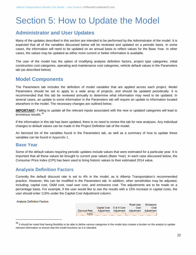
Analysis Definition Factors Currently the default discount rate is set to 4% in the model, as is Alberta Transportation’s recommended practice. However, this can be modified in the Parameters tab. In addition, other sensitivities may be adjusted, including: capital cost, O&M cost, road user cost, and emissions cost. The adjustments are to be made on a percentage basis. For example, if the user would like to see the results with a 15% increase in capital costs, the user should enter 115% under the Capital Cost Adjustment column.

38 It should be noted that having flexibility to be able to define various categories in the model also creates a burden on the analyst to update relevant information to ensure that the model functions as it is intended.

22

Alberta Transportation Benefit Cost Model - User Guide to ATBenefitCostModelV2.xlsx Discount Rate (4% Default)

The discount rate used to calculate the Discounted Total Cumulative Costs (in Present Values) and Breakeven Point is set by the user. There is no ‘right’ discount rate. However, the rate should reflect the risk and time value of money from the perspective of the provincial government. If there is an official discount rate that the GOA adopts, this should be used for the analysis. At the time of writing (2016) the default discount rate for all Alberta Transportation projects is 4%. Generally, the public sector uses a lower discount rate than the private sector because it is argued that generally the public sector can be more patient to receive a return on investment than the private sector. In choosing a discount rate, current economic conditions, inflation and risk of the investment should be considered. At the time of writing (2016), inflation is low reducing the time value of money costs. As a result, a relatively historically low discount rate of 4% could be used for the ‘do minimum’ alternative.

It has long been the practice of Alberta Transportation to use a 4% discount rate for projects. This is in contrast to the Canadian Federal Treasury Board Benefit Cost Guidelines that recommend 10%.39 Project Type Categories

There are default values for running (or design) speed and asset life for each project type. Defaults provided are intended to be a guide to assist with estimating timeline of rehabilitation and reinvestment costs. However, the analyst may alter these values if necessary. Up to 10 different project types may be defined.

Initial Construction Cost Categories The analyst can define up to 8 different types of construction costs. The Construction Cost Categories are linked to the Alt # tabs. In the Alt # tabs, the analyst may enter the construction costs for each construction cost category. The user should define Construction Cost categories that will be useful for each analysis.

Operating & Maintenance Cost Categories (Specified Maintenance) The user may use these defined categories, the fixed Scheduled Maintenance categories described below, or a combination of the two. Cost category usage is defined in the Alt # tabs. A description of how to define the categories can be found in Section 3: Operating and Maintenance Cost.

39 The Treasury Board's 1976 Benefit-Cost Analysis Guide states that the discount rate for federal government projects is 10% in real terms (i.e., when using constant dollars). The Guide also calls for sensitivity analysis (see Section 9.4.1) using real discount rates of 5% and 15%. GUIDE TO BENEFIT-COST ANALYSIS IN TRANSPORT CANADA, Transport Canada, TP11875E, September 1994.

23

Alberta Transportation Benefit Cost Model - User Guide to ATBenefitCostModelV2.xlsx The analyst can define up to 5 different types of operating and maintenance costs. The Operating & Maintenance Cost Categories are linked to the Alt # tabs. The analyst will enter the operating and maintenance costs for each category. If using Specified Maintenance, the analyst should define Operating and Maintenance Cost categories that will be useful for each analysis.

Maintenance Cost Categories by Surface Type (Scheduled Maintenance)

There are three fixed Scheduled Maintenance Cost Categories. These cost categories are used to calculate maintenance costs given the surface type. The Maintenance Cost Categories are linked to the Alt # tabs. The Administrator should check to ensure that the most current values for these Maintenance Cost categories are in the model. These values are contained in the Maintenance tab (array G15:I134).40

Vehicle Default Values

The analyst can define up to 10 different vehicle types in the Parameters tab. There are 7 default vehicles currently in the model, and should be left as is unless the analyst has differing project specific information. For each vehicle type, the following information is required: average vehicle occupancy, business and non-business costs/hr, fuel and non-fuel operating costs, fuel efficiency and an assigned vehicle type (auto/truck). The analyst should define the vehicle types to reflect the mix of vehicles using Alberta roads.

The Traffic Alt # tabs, Project Definition tab, and Alt # tabs use the Vehicle Type definitions to perform various calculations. No updates are required in these tabs as a result of a change in the Vehicle Type definitions. Occupancy

Average occupancy rate for light vehicles as reported by Natural Resources Canada (2009)41 is 1.68. This has been applied to each of the passenger vehicle, RV, single unit truck vehicles.

40 It is not expected that the Maintenance Cost categories will change. 41 2009 Canadian Vehicle Survey Summary Report, Natural Resources Canada, Office of Energy Efficiency, page 54. http://oee.rncan.gc.ca/publications/statistics/cvs09/index.cfm

24

http://oee.rncan.gc.ca/publications/statistics/cvs09/index.cfm


Occupancy information for other vehicle types, including medium and heavy vehicles and buses are ‘assumed’ values.

Work Business Cost $/hr

The Work Business Cost per hour reflects the cost of traveller time for work related trips. The average hourly wage rate in Alberta has been used for non-commercial vehicles ($24.84)42 adjusted for inflation to 2014 ($26.00), the truck driver rate (24.69)43 adjusted for inflation to 2014 ($26.00) has been used for commercial trucking and bus driver rate ($20.11)44 adjusted to 2014 ($21.00) for buses.45 All data has been drawn from Alberta Learning Information Service (ALIS) WageInfo website.46

Other/Leisure Cost $/hr The travel time costs for non-business travel associated with leisure or other trips is typically lower than for

business or work trips. It has been estimated by the US Department of Transport that non-business travel time values range between 50% and 70% of wages (or the business/work value of travel time).47 The lower end of this range is supported by a more recent study prepared for Transport Canada where the ‘overall or base Valuation of Travel Time Savings would be 50% of the average wage rate’.48 As a result, it has been assumed that ‘other’ (leisure) travel time costs would be 50% of the rate used for ‘business/work’ travel time.

Non Fuel Vehicle Operating Cost (California [Fuel & Non-Fuel]) Calculation

The California (Fuel & Non-Fuel) Vehicle Operating Cost calculation is based on the approach used in the CalTrans Benefit Cost Model. In this model vehicle operating costs are broken into fuel and non-fuel operating costs. Non-fuel operating costs include all vehicle operating costs, as measured by the average cost per distance (km).49 Values are reported for two vehicle classes: autos and trucks. These values reported by the CalTrans model have been modified to reflect metric units and updated to 2012 values.

For example, if the non-fuel vehicle cost per mile is 0.239 $/mi for 2007, it is multiplied by 0.621 (1km = 0.621 mi) to get 0.148 $/km. This value is then updated to 2014 by multiplying 0.148 $/km by the inflation index (CPI), yielding a final value of 0.159 $/km. The non-fuel costs of heavy vehicles is reported by Barton & Associates to be approximately 0.2154 per tonne-km or passenger-km.50 While the cost per tonne-km or passenger-km is similar to the converted CalTrans estimate for trucks, it is noted that the units are not an exact match. The Barton & Associates figure has been updated to 2014 using the CPI inflation index, yielding a final value of 0.0244 $/km.

42 http://alis.alberta.ca/pdf/wageinfo/2011_AWSS_Wages_By_Industry_and_Region.pdf 43 http://alis.alberta.ca/wageinfo/Content/RequestAction.asp?SearchContent=truck +driver&aspAction=GetWageKeyWordSearchResult&format=html&Page=SearchKeyword&RegionID=20 44 http://alis.alberta.ca/wageinfo/Content/RequestAction.asp? aspAction=GetWageDetail&format=html&RegionID=20&NOC=7412 45 All values have been rounded to the nearest dollar. 46 http://alis.alberta.ca/wageinfo/Content/RequestAction.asp?format=html&aspAction=GetWageHomePage&Page=Home 47 USDOT (1997), Departmental Guidance on the Evaluation of Travel Time in Economic Analysis, memo, USDOT (www.fhwa.dot.gov); used in STEAM software (www.ota.fhwa.dot.gov/steam). 48 Anming Zhang, Anthony E. Boardman, David Gillen and W.G. Waters II, Towards Estimating the Social and Environmental Costs of Transportation in Canada, Transport Canada, Aug 2004, page 20. 49 California Life-Cycle Benefit/Cost Analysis Model (Cal-B/C), Version 4.0, February 2009 50 Estimation of Costs of Heavy Vehicle Use per Vehicle-Kilometre in Canada, Transport Canada T80808-05-0326, by Barton & Associates in association with Logistics Solution Builders Inc., December 2006, page 61. This cost estimate is for tractor-trailer operations in uncongested conditions. The calculations in Barton include fuel costs which have been taken out of figures reported here.

25

http://alis.alberta.ca/pdf/wageinfo/2011_AWSS_Wages_By_Industry_and_Region.pdf

http://alis.alberta.ca/wageinfo/Content/RequestAction.asp?SearchContent=truck

http://alis.alberta.ca/wageinfo/Content/RequestAction.asp

http://alis.alberta.ca/wageinfo/Content/RequestAction.asp?format=html&aspAction=GetWageHomePage&Page=Home

http://www.ota.fhwa.dot.gov/steam)

Alberta Transportation Benefit Cost Model - User Guide to ATBenefitCostModelV2.xlsx Fuel Cost/litre (California [Fuel & Non‐Fuel] Vehicle Operating Cost Calculation)

Gasoline: Fuel costs have been sourced from AlbertaGasPrices.com, which provides a compendium of gas prices across Alberta. The current average cost of gasoline is $1.15 per litre and it has averaged approximately $1.15 per litre in 2014 (January to April).51

Diesel: Using the same source, current diesel prices have been tracking above gasoline prices by about 10¢ per litre. As a result, fuel costs for vehicles types that primarily use diesel have been updated to $1.25 per litre.52

Calibration to Department Rate The vehicle operating costs for the California (Fuel and Non-Fuel) approach have been calibrated to the Department’s vehicle operating cost pay rate of $0.505/km. Alberta Transportation’s Finance Director has advised that the rate is established by the Treasury Board and Finance, and that the factors that went into obtaining the rate include fuel, maintenance, insurance, and amortization cost.

Fuel Taxes/litre (California [Fuel & Non‐Fuel] Vehicle Operating Costs) As taxes are a transfer53 they cannot be included in the benefit cost analysis. Using retail fuel prices thus requires

that taxes be deducted. The current tax rates for fuel in Alberta are 24.554 cents per litre plus GST.54

Fuel Efficiency (litre/100 km) (California [Fuel & Non‐Fuel] Vehicle Operating Costs)

Average fuel consumption is reported by Natural Resources Canada (NRCan) (2009)55 for three vehicle classes56 (Light Vehicles, Medium Trucks and Heavy Trucks) as follows nationally (and regionally). The Alberta rates are used in the model as follows:

Light Vehicles (Gasoline): 10.7 litres/100 km (Alberta Rate 11.3)57 Light vehicles include: cars, station wagons, vans, SUVs, pickup trucks, and other vehicles (straight trucks, tractor trailers and buses),

Light Vehicles (Diesel): 10.6 litres/100 km (defined as above)

Medium Trucks (Diesel): 24.4 litres/100 km (Alberta Rate 22.0)58 (defined as above)

Medium Trucks59 (Gasoline): 25.1 litres/100 km. Medium trucks are defined as having a gross vehicle weight between 4.5 and 15 tonnes

Heavy Trucks60 (Diesel): 33.4 litres/100 km (Alberta Rate 33.1)61 Heavy trucks are defined as having a gross vehicle weight of 15 tonnes or more

51 http://www.albertagasprices.com/Retail_Price_Chart.aspx 52 Given that fuel costs can fluctuate dramatically from month to month and season to season, it is recommended that a reasonable estimate be included in the model by the Administrator and this be used for all analysis until the next update. Where the current trend in fuel prices is dramatically different that the base values used in the model, this may be run as a sensitivity to determine what the impact would be on the Benefit Cost Analysis results. 53 Taxes can be seen as a transfer from consumers to Government. If they were to be included in the analysis, the taxes would be doubly counted. For this reason, they must be subtracted from the total fuel cost. 54 http://gasbuddy.com/Can_Tax_Info.aspx 55 2009 Canadian Vehicle Survey Summary Report, Natural Resources Canada, Office of Energy Efficiency, page 9. http://oee.rncan.gc.ca/publications/statistics/cvs09/index.cfm 56 Ibid, page 23 57 Ibid, page 19 58 Ibid, page 20 59 Ibid, page 31. 60 Ibid, page 31. 61 Ibid, page 21

26

http://www.albertagasprices.com/Retail_Price_Chart.aspx

http://gasbuddy.com/Can_Tax_Info.aspx

http://oee.rncan.gc.ca/publications/statistics/cvs09/index.cfm


Fuel consumption for new passenger vehicles (2012) has been calculated for 83 vehicles using Natural Resources Canada’s Fuel Consumption Ratings.62 Of these, 10 are hybrid vehicles and have a rated average fuel consumption of 4.93 litres/100 km. The remaining new cars have a rated fuel consumption of 6.59 litres/100 km. Because the current fleet of light vehicles as defined by Natural Resources Canada is about half cars and station wagons and half vans, SUVs and pickup trucks, and about only 20% of these vehicles are less than 3 years old, the average fuel consumption for passenger vehicles can be expected to lie between 6.6 (as calculated for new non hybrid vehicles) and 10.7 as reported by NRCan. Without access to the raw data to be able to estimate the actual value, the mid-point of these two estimates is currently reported for non-hybrid passenger vehicles (8.5 litres/100 km).

Other alternative sources of fuel efficiency were also reviewed. Examples of these include the following:

Using Natural Resources Canada’s Fuel Consumption Ratings for new pickup trucks (2012) yielded an average of 9.61 litres/100 km63. This is very close to the average report for light vehicles (2009).

Fuel consumption for intercity buses is reported by Barton & Associates to be 37.5 litres/100 km.64

Road User Gradient Factor Categories (Texas [Curvature & Gradient] Vehicle Operating Costs) The Texas (Curvature & Gradient) approach to calculating road user costs uses gradient and curvature costs assigned by vehicle type. This approach uses factors that originated in part from data compiled by the Texas Research and Development Foundation in 1982 for the Federal Highway Administration. For the Texas (Curvature & Gradient) Alberta Transportation Benefit Cost Model, these numbers were converted to 1988 Canadian dollars using Alberta consumer prices for items such as fuel, oil, tires, depreciation, etc. From there further increases were applied to the numbers based on the Transportation Price Index from 1988 to 2012. These 2012 factors are used in the new version of the model.65 The calculations associated with the Texas (Curvature & Gradient) approach to estimating road user costs are completed in the RUC Alt# tabs. The data used to perform these calculations (updated to 2012) is in the RUC Alt1 tab as follows:66

Gradient Costs: RUC Alt1 beginning at A294. Curvature Costs: RUC Alt1 beginning at AY6.

Collisions67

Major Injury: 2006-2010 average (Alberta Transportation, Traffic Safety Branch) of Persons Injured divided by the number of Non-Fatal Injury Collisions (Table 1.1 page 2, 2010 Traffic Collision Summary). The proportion of injury collisions that are ‘serious’ are estimated based on national data (Canadian Motor Vehicle Traffic Collision Statistics: 2009)68 where the number of seriously injured and total injured is available. This rate has declined steadily from the early 90’s from about 10% of all injuries to 6.6% in 2009. Applying this rate to the Alberta non-fatal injury rate (the number of people in a collision with a non-fatal major injury) is 0.09.

62 Natural Resources Canada Fuel Consumption Ratings http://oee.nrcan.gc.ca/cars-light-trucks/buying/fuel- comsumption-guide/fuel-consumption-ratings/17771 63 Ibid 64 Estimation of Costs of Heavy Vehicle Use per Vehicle-Kilometre in Canada, Transport Canada T80808-05-0326, by Barton & Associates in association with Logistics Solution Builders Inc., December 2006, page 27. 65 Benefit Cost Analysis - Vehicle Running Costs, Alberta Transportation & Utilities, Traffic Engineering Branch, January 1989. 66 The calculations used for the other alternatives are linked to the source data in the RUC Alt1 tab. 67 Alberta Traffic Collision Data is contained in Appendix 2. 68 Transport Canada TP 3322 Cat. T45-3/2009 2011 http://www.tc.gc.ca/eng/roadsafety/tp- tp3322-2009-1173.htm#t6

27

http://oee.nrcan.gc.ca/cars-light-trucks/buying/fuel-

http://www.tc.gc.ca/eng/roadsafety/tp-


Minor Injury: Same average used for Minor Injury as Major/Serious Injury. As above, national data regarding the proportion of injuries that are ‘serious’ has been used to estimate the number of ‘moderate’ injuries, estimated to be 93.4% in 2009. Applying this rate to the Alberta non-fatal injury rate, the 2012 base year number of people in a collision with a non-fatal minor injury is 1.27.

Collision Rates

The collision rate information provided for 2010 was broken down into 6 categories as defined below. The rates reported here are based on 2010 data. As of 2011 the Office of Traffic Safety is reporting collision rates for Property Damage Only (PDO) when the value of the damage is $2,000 or more as compared to the previous data which used a threshold of $1,000 for reporting purposes.69

The total number of collisions in Alberta in 2010 was 151,298 (Alberta Transportation, Traffic Safety).70 The model utilizes collision rates per hundred million vehicle kilometres travelled for highway type and location (urban/rural) where this information is available.

The model can accept differing collision rates for each of 5 combinations of surface type (gravel/paved) and road type (2 lane, 4 lane undivided, 4 lane divided expressway, 4 lane divided freeway). If collision data is available for a specific road, these rates can be input into the model as project specific values. Collision rates can be obtained from the graphs included in the collision rates tab; if the rates are unavailable for the situation in question then the default values may be used. The average collision rates for Alberta in 2010 were as follows71:

Collision Costs

All collision costs used in the model have been provided by the Alberta Transportation Traffic Safety Branch. These estimates are based on work being done across Canada with Transport Canada, which is yet to be finalized. Based on the work to date, the Collision Costs by Type of collision (average for 2006-2011) have been inflated to reflect 2014 values using the CPI inflation index, resulting in values as follows: The social cost values reflect the total cost for each category of collision severity.72

69 Note that the threshold for reporting Property Damage Only (PDO) collisions increased from $1,000 to $2,000 January 1, 2011. 70 Alberta Traffic Collision Statistics 2010, Alberta Transportation, Traffic Safety, page 8. 71 Note that the Urban Collision Rate and proportion of collisions by Type of Collision for 6+ Lanes was not available and the Rural data has been used as a proxy for this data. 72 For example, a collision involving a fatality will include the estimate for the fatality, injury and property damage costs.

28

Alberta Transportation Benefit Cost Model - User Guide to ATBenefitCostModelV2.xlsx Emission Costs by Type

The vehicle emissions component was modelled after the California Life-Cycle Benefit/Cost Analysis Model73

which incorporates values for six different emission categories. The values for each emissions component were taken from this model, converted from gram/mile to tonne/km, and were updated to 2014 using CPI.

All values are cost per tonne of emissions.

CO (Carbon Monoxide): $96.50 CO2 (Carbon Dioxide): $40.00 NOx (Nitrogen Oxides): $30,000.00 PM10 (Particular Matter): $244,000.00 SOx (Sulphur Oxides): $102,000.00 VOC (Volatile Organic Compounds): $2,000.00

Note: benefits from reducing air emissions are location specific. This document uses American, urban-area values that might not accurately reflect potential benefits in Alberta. However, for this model’s purposes, the user can still use the default provided values. Emission costs vary by the average running speed of the vehicle. The Emissions tab uses the emission factors for various vehicle types defined in the California Life-Cycle Benefit/Cost Analysis Model (Cal-B/C). The CalTrans model defines emissions by speed as measured by miles/hr. These units have been converted to km/hr outside the model (emissionsConvV1b.xlsx). Example:

Total emission costs / km = summation of six emission categories / km Emission costs ($/km) = Σ $ / tonne * grams of emissions / km / 1,000,000 1. Passenger Car, Average speed of 110 km/h

The fuel consumption rate for passenger vehicles at 110 km/h is ~12.42 L/100 km, converted and rounded from the corresponding imperial value provided by CalTrans (see FuelConsump tab in the model). 110 km/h CO CO2 NOx PM SOx VOC Total grams/km 4.8380 449.620 0.5010 0.0340 0.0046 0.3640 455.3616 weighting 0.0106 0.98739 0.0011 0.000075 0.0000101 0.000799 1 cost ($/km) 0.00047 0.0180 0.0150 0.0083 0.0005 0.0007 0.0430

A passenger car travelling at 110 km/h with fuel consumption rate of 12.42 L/100km using 1000L of fuel (~$1,150) could travel 8,052 km, leading to a cost of $346 for total emissions of 3,666,572 g (3.7 T). 2. Passenger Car, Average speed of 60 km/h

The fuel consumption rate for passenger vehicles at 60 km/h is ~10.47 L/100 km, converted and rounded from the corresponding imperial value provided by CalTrans (see FuelConsump tab in the model). 60 km/h CO CO2 NOx PM SOx VOC Total gms/km 4.0012 377.16 0.4251 0.0335 0.0039 0.3153 381.9390 weighting 0.0105 0.9875 0.0011 0.0000877 0.00001 0.000826 1 cost ($/km) 0.0004 0.0151 0.0128 0.0082 0.0004 0.0006 0.0374

A passenger car travelling at 60 km/h with fuel consumption rate of 10.47 L/100km using 1000 L of fuel (~$1,150) could travel 9,551 km, leading to a cost of $357 for total emissions of 3,647,899 g (3.6 T).

73 California Life-Cycle Benefit/Cost Analysis Model (Cal-B/C), Version 4.0, February 2009 29


Appendix 1: Summary of Model Variables

The variables in the Parameters tab are itemized in the table below. Values highlighted (red) in this table indicate an external source should be consulted to determine the default value. The source and process for updating these default values is provided for each variable in the section below the table.

Component Variable Definition Information Source Links Base Year Used by the model as the

Base Year for all time sensitive calculations

Current year All components with a timeline

Analysis Definition Factors

Discount Rate Used to discount costs to their present day values.

User (4% is AT’s default value)

All discounted costs

Capital Cost Adjustment

Used to determine the change in capital costs as a sensitivity analysis.

User - optional Applied to both capital and rehab costs.

O&M Cost Adjustment

Used to determine the change in O&M costs as a sensitivity analysis.

User – optional Applied to O&M costs.

Road User Cost Adjustment

Used to determine the change in road user costs as a sensitivity analysis.

User – optional Applied to vehicle operating costs and travel time costs.

Emission Cost Adjustment

Used to determine the change in emission costs as a sensitivity analysis.

User – optional Applied to vehicle emissions costs.

Project Type Categories

Type of Project (up to 10)

Default data for running speed and project life.

User Alt# design speed (info only)

Default running speed

Provided as a guide when defining the Alternative in Alt#.

User Provided as information in Project Definition.

Project life Provided as a guide for completing rehab costs in ProjectCostsAlt# tabs.

User estimates project life. Provided as information

Construction Cost Categories

Type of construction cost (up to 8)

To separate the costs of the project into logical categories for typical projects.

User - based on typical projects & where necessary, project specific categories (e.g. enviro. mitigation)

Project Costs tabs

Operating Cost Categories

Type of operating cost (up to 5)

To separate the operating and maintenance costs of the project into logical categories for typical projects.

User - based on typical projects & where necessary, categories can be defined (e.g. on-going environmental mitigation costs)

Project Costs tabs

Vehicle Types, Occupancy & Unit Costs for Time

Vehicle Type (up to 10)

To separate the costs that are vehicle specific.

User defined All vehicle-related costs and forecasts of traffic.

Occupancy No. of people per vehicle for Travel Time Costs.

Natural Resources Canada (light vehicles)

Travel time costs

Work/Bus$/hr Value of time for work and business trips.

WageInfo (Alta) & Transportation Cost/Benefit Analysis II

Travel time costs

Other $/hr Value of time for non-work trips.

WageInfo (Alta) & Transportation Cost/Benefit Analysis II

Alberta Transportation Benefit Cost Model - User Guide to ATBenefitCostModelV2.xlsx Component Variable Definition Information Source Links Texas (Curvature & Gradient) Method

Various The Texas (Curvature & Gradient) Vehicle Operating Costs are based on work completed by AT in 1989.

Benefit Cost Analysis – Vehicle Running Costs, Alberta Transportation and Utilities.

Vehicle Values by Road Type: RUC Alt 1 (AY42:BA47)

California (Fuel & Non-Fuel) Method

Non Fuel Vehicle Cost $/hr

All user costs (except fuel) associated with operating a vehicle.

Cal-B/C February 2009 advanced to 2011 using CPI

California (Fuel & Non-Fuel) vehicle operating costs

Fuel Cost / Litre Average price of fuel typical for the vehicle type (e.g. gasoline / diesel).

2012 average Alta fuel costs (AlbertaGasPrices.com)


Fuel Efficiency (Litre/100 km)

Litres of fuel consumed per 100 km travelled at average speed of 105 km/hr (highway driving)

Natural Resources Canada


Vehicle Category Will be either Auto or Truck and used to adjust fuel consumption by average vehicle speed

User (based on the vehicle type specified by the user)


Growth Driver Types (3)

Linear, Traffic Growth, and Exponential

Categories defined in the model to project O&M costs

Cannot be changed by analyst.

Traffic Direction

Two direction categories: 1 way, 2 way

Categories defined in the model used to allocate gradient costs to traffic on each road segment


Gradient costs per road segment

Collision Categories

3 categories: fatality, serious injury, moderate injury

Categories defined in the model Cannot be changed by analyst.

Used to calculate collision costs

Collision Rates by Type of Collision

Surface Type / Road Type

The collision rate and distribution of collisions by can be varied across 5 combinations of surface and road types



Collision Rate Number of collisions per 100 million vehicle kms. See Appendix 2 for collision rate information from 2006-2011.

Traffic Safety Used to calculate collision costs

Fatality The proportion of total collisions involving a fatality.


Injury The proportion of total collisions involving an injury.


Property Damage Only

The proportion of total collisions involving only property damage.


Collision Costs by Type

Social costs (fatality/injury) and PDO costs

The average cost per person by collision type

Categories cannot be changed by analyst.


Fatality Social cost of each person involved in a fatal collision


Serious Injury Social cost of each person involved in a serious injury


Moderate Injury Social cost of each person involved in a moderate injury


Emission Costs Type

Type of Emission Label for the type or category of emission.

At Department’s discretion

Used to calculate emission costs

Cost per Tonne The social cost of each emission category.

California Life-Cycle Benefit/Cost Model

Used to calculate emission costs


Appendix 2: Alberta Traffic Collision Data

Alberta Traffic Collisions 2006-2011

Urban 2011 2010 2009 2008 2007 2006

N % N % N % N % N % N % Fatal Collisions 75 0.1 77 0.1 83 0.0 105 0.08242 130 0.1 119 0.1 Non-Fatal Injury Collisions 9897 8.8 9902 8.1 10534 0.9 12074 9.47768 13638 11.1 14267 12.8 Property Damage Collisions 102064 91.1 112155 91.8 1175579 99.1 115215 90.4399 109395 88.8 96825 87.1 Total Urban Collision 112036 100.0 122134 100.0 1186196 100.0 127394 100.0 123163 ,.. 100.0 111211 100.0

Alberta Transportation Office of Traffic Safety

August 2013

Alberta Total 2011 N

%

2010 N

%

2009 N

%

2008 N

%

2007 N

%

2006 N

%

Fatal Collisions 285 0.2 307 0.2 302 0.2 375 0.2 402 0.3 404 0.3 Non-Fatal Injury Collisions 13909 10.0 13552 9.0 14246 9.1 16153 10.2 17857 11.6 18831 13.2 Property Damage Collisions 124985 89.8 137430 90.8 142678 90.7 141527 89.5 135642 88.1 123357 86.5 Total Reportable Collisions 139179 100.0 151289 100.0 157226 100.0 158055 100.0 153901 100.0 142592 100.0

Rural Highways

2011

2010

2009

2008

2007

2006

N % N % N % N % N % N % Fatal Collisions 170 0.9 181 0.9 173 0.9 212 1.0 211 1.0 220 1.0 Non-Fatal Injury Collisions 2937 15.2 2591 13.0 2582 13.3 2834 13.7 3073 14.4 3245 15.3 Property Damage Collisions 16244 83.9 17096 86.0 16708 85.8 17655 85.3 17995 84.6 17766 83.7 Total Rural Highway Collisions 19351 100.0 19868 100.0 19463 100.0 20701 100.0 21279 100.0 21231 100.0


0.0

20.0

40.0

60.0

80.0

100.0

120.0

140.0

0 5000 10000 15000 20000 25000 30000 35000 40000 45000

Col

lisio

n R

ate

(per

100

mill

ion

vehi

cle

kms)

AADT

4-Lane Divided, at Grade, Rural Collision Rates

0.0

50.0

100.0

150.0

200.0

250.0

300.00

101

201

301

401

501

601

701

801

901

1001

1101

1201

1301

1401

1501

2001

2501

3001

3501

4001

4501

5001

5501

6001

Colli

sion

Rat

e (p

er 1

00 m

illio

n ve

hicl

e km

s)

AADT

2 Lane Paved Undivided Highway Rural Collision Rates Varying by Width of Roadway

0 to <7.5 m

7.5 to 8.5 m

8.5 to 9.5 m

9.5 to 10.5

10.5 to 11.5 m

11.5+ m


30.0

35.0

40.0

45.0

50.0

55.0

60.0

65.0

70.0

10000 15000 20000 25000 30000 35000 40000 45000

Col

lisio

n R

ate

(per

100

mill

ion

vehi

cle

kms)

AADT

Divided Highway, Not at Grade (Freeway), Rural Collision Rates

20.0

30.0

40.0

50.0

60.0

70.0

80.0

90.0

0 10000 20000 30000 40000 50000 60000 70000 80000 90000

Col

lisio

n R

ate

(per

100

mill

ion

vehi

cle

kms)

AADT

6+ Lanes (Freeway) Rural Collision Rates


0

50

100

150

200

250

300

0 2000 4000 6000 8000 10000 12000

Col

lisio

n R

ate

(per

100

mill

ion

vehi

cle

kms)

AADT

Undivided Highway Urban Collision Rates

0

50

100

150

200

250

300

0 5000 10000 15000 20000 25000 30000 35000 40000 45000 50000

Colli

sion

Rat

e (p

er 1

00 m

illio

n ve

hicl

e km

s)

AADT

Divided Highway Urban Collision Rates

benefit cost model user guide - alberta · alberta transportation benefit cost model - user guide...

Documents