lable at ScienceDirect

Renewable Energy 86 (2016) 819e830

Contents lists avai

Renewable Energy

journal homepage: www.elsevier .com/locate/renene

Benefits of solar forecasting for energy imbalance markets

Amanpreet Kaur, Lukas Nonnenmacher, Hugo T.C. Pedro, Carlos F.M. Coimbra*

Department of Mechanical and Aerospace Engineering, Jacobs School of Engineering, Center for Energy Research and Center of Excellence in RenewableResource Integration, University of California San Diego, La Jolla, CA 92093, USA

a r t i c l e i n f o

Article history:Received 24 March 2015Received in revised form30 July 2015Accepted 2 September 2015Available online xxx

Keywords:Solar forecastingReal-time marketEnergy imbalance marketReserves

* Corresponding author.E-mail address: ccoimbra@ucsd.edu (C.F.M. Coimb

http://dx.doi.org/10.1016/j.renene.2015.09.0110960-1481/© 2015 Published by Elsevier Ltd.

a b s t r a c t

Short term electricity trading to balance generation and demand provides an economic opportunity tointegrate larger shares of variable renewable energy sources in the power grid. Recently, many regulatorymarket environments are reorganized to allow short term electricity trading. This study seeks to quantifythe benefits of solar forecasting for energy imbalance markets (EIM). State-of-the-art solar forecasts,covering forecast horizons ranging from 24 h to 5 min are proposed and compared against the currentlyused benchmark models, persistence (P) and smart persistence (SP). The implemented reforecast ofnumerical weather prediction time series achieves a skill of 14.5% over the smart persistence model.Using the proposed forecasts for a forecast horizon of up to 75 min for a single 1 MW power plant re-duces required flexibility reserves by 21% and 16.14%, depending on the allowed trading intervals (5 and15 min). The probability of an imbalance, caused through wrong market bids from PV solar plants, can bereduced by 19.65% and 15.12% (for 5 and 15 min trading intervals). All EIM stakeholders benefit fromaccurate forecasting. Previous estimates on the benefits of EIMs, based on persistence model are con-servative. It is shown that the design variables regulating the market time lines, the bidding and thebinding schedules, drive the benefits of forecasting.

© 2015 Published by Elsevier Ltd.

1. Introduction

The electricity system is undergoing an inevitable change toaddress increased variability in generation and net load, introducedby intermittent generators, mainly wind and solar. Many ap-proaches to mitigate the adverse effects of ramping have beenproposed, e.g. increased storage capabilities, resource and net loadforecasting, demand response, etc. The core of all solutions forintegrating higher levels of variable wind and solar generation is toincrease the flexibility options available in the grid [1,2]. Recently,regulating authorities in several jurisdictions reorganized themarket environments to allow flexible energy trading schedules,designed to better exploit spatial and temporal diversity in gener-ation and demand. Historically, this reorganization started inNorthern Europe by allowing short-term, cross-border electricitytrading, driven by the need to integrate increasing shares of vari-able wind generation.

In October 2014, the Energy Imbalance Market (EIM) in theWestern Interconnection was opened in United States of America

ra).

interconnecting over 30 participating balancing authorities (BAs) inUSA and Canada. This allows for generation and demand balancingacross Balancing Authority Areas (BAA) on 15 min and 5 min time-scales with California Independent System Operator (CAISO) over-sight. Previous to the opening, all the Balancing Authorities (BA)were responsible to balance generation and demand for their ownarea. Now, the ISO can dispatch and share resources across theparticipating BAAs to balance energy of all BAs. All EIM marketparticipants are mandated to provide a continuous feed of specifiedforecasts to the ISO. Energy imbalances caused by errors in theforecasts and bidding are settled by the defined settling regulatione.g. according to the United States Federal Energy RegulatoryCommission (FERC) Order 890, for intermittent renewable gener-ators, imbalances greater than 7.5% or 10 MW are settled at 125%incremental cost or 75% decremental cost of providing the imbal-ance energy. In contrast to the dominance of wind as intermittentgenerator in Northern Europe, solar is the dominating intermittentenergy source in many regions in theWestern Interconnectionwithtremendous expected growth rates (e.g. California).

On this background, this study aims to analyze and quantify thebenefits of solar forecasting for EIM operations. To achieve this,solar forecasts are implemented to cover all necessary forecasthorizons for EIM operations. All implemented forecasts are state-

A. Kaur et al. / Renewable Energy 86 (2016) 819e830820

of-the-art methodologies based on broadly available methods,relying on low-cost instrumentation and publicly available data.The contributions of this study are: 1) reforecast methodology toforecast day-ahead global irradiance 2) features based optimizedshort-term solar forecasting 3) analysis of solar forecast errors forthe forecast horizons related to electricity markets, especially theshort-term EIM market in the Western Interconnection and 4)detailed analysis on the role of solar forecasting in EIM in terms ofuncertainty and estimation of flexibility reserves from theperspective of market operator and participants.

More detailed discussion on the EIM and previous work on solarresource forecasting are provided in Section 2, the data sets usedare described in Section 3, methods for solar forecasting areexplained in Section 4, results are discussed in Section 5, the valueof forecasting for EIM is shown in Section 6 and conclusions aredrawn in Section 7.

2. Energy imbalance markets

2.1. Goals

The main objective for the introduction of EIMs is to reduceimbalances between demand and generation without ancillaryservices or additional reserves by enabling regulated, short-termenergy trading between interconnected balancing areas. WithoutEIMs, resources were not shared between the balancing areas. Theindividual balancing area authorities had to schedule and keepoperating reserves to handle imbalances. For the EIM in theWestern Interconnection, after scheduling for 15 min market, the5 min market is executed to automatically procure resources tobalance expected imbalances between generation and demand in5 min time intervals. Taking the advantage of increasedgeographical diversity in generation and load profiles, the mainbenefits of this market are reduced operating reserves capacity,enhanced reliability, reduced costs and automatic dispatch, andreal-time visibility.

2.2. Previous work

This section covers a short summary of previous work, relevantfor EIMs. A review on real-time markets is presented in Ref. [3]. Anoverview of previous EIM studies can be found in Ref. [4]. Theyinclude a comparison of market regulations based on assumptions,annual benefits, and geographic scope. The study includes benefitsof the implemented EIM between ISO and PacifiCorp. The impactfor EIM, for grids with high levels of wind penetration, was studiedin Ref. [5]. They show that the introduction of EIMs enables reserverequirement reductions which is beneficial for all EIM participants.Furthermore, they show that the failure or refusal of participationby as little as one entity can reduce the benefits for all other par-ticipants in the market. Using forecasts as a decision variable thebidders and market operator can commit or de-commit in case ofhigh or low energy production [6]. An evaluation of energy balanceand imbalance settlements in Europe is presented in Ref. [7].

A general framework for analyzing various components ofmarket participation for wind generators was proposed in Ref. [8].They discuss the value of information contained in forecasts forgrids with high wind penetration. Conclusions cover that fore-casting has a high economic value for variable wind energy sources.For current status of wind penetration in CAISO, investment inshort-term wind forecasting is precarious, whereas in future sce-narios with high wind penetration levels, forecasting can evolveinto an important decision variable for real-time market operation,e.g. economic dispatch in the CAISO area [9]. A detailed analysis onorganized markets in the Western Interconnection can be found in

Ref. [10]. It highlights the factors influencing the success of EIMs,such as cost allocation, transmission rights, participation of variousBAAs, stakeholders and discusses the alternatives to organizedmarkets, for instance Intra-hour Transaction Accelerator Platform,the Dynamic Scheduling System, Balancing Authority Reliability-based Control, Area Control Error Diversity Interchange, EnhanceCurtailment Calculator, etc. While these alternative market setupsmight be beneficial in certain cases, the regulating authoritiesdecided to operate an EIM in the Western Interconnection. Thefocus of our work is the EIM in the Western Interconnection in theUnited States.

Most of the studies on the impact of EIM on Western andEastern Interconnection assume forecasts to be persistent [6].However, there has been tremendous progress in the field of solarenergy resource forecasting over the past decade. Hence, previousstudies provide a conservative estimate of reserves. In this study,we seek to quantify the benefits of state-of-art-solar solar forecastsfor the EIM. The next section covers key design variables of EIMsand current solar forecasting methods that can be utilized for EIMparticipation and operation.

2.3. Market design variables

The two fundamental concepts for energy imbalance marketsare balance responsibility and imbalance settlements [7]. Balancingresponsibility covers the processes from market opening, to bind-ing and market execution. The key variables for balance re-sponsibilities are: (1) program time unit (PTU), defined as the timewindow for which bids are submitted and base schedules areawarded. (2) Scope of balancing, defined as the magnitude ofnecessary generation change. (3) Gate closure time (GCTp/o);defining the time when the option to submit or modify a bid ex-pires. The GCTp is for market participants while the GCTo is timewhen schedules are binded from the operator. (4) Types of imbal-ances, depending on if over- or under-generation occurs. (5) Closed(zero imbalance) or open (occurring imbalance) portfolio positionsand (6) look ahead time (LAD), defining the ahead time horizonconsidered for running the optimization to schedule awards.

The design of imbalance settlements define the detailed setup ofpenalties associated with wrong forecasts and market bids. Detailsabout imbalance settlements can be found in Ref. [7]. In general, itcovers the frequency of settlements, regulations and pricing ofimbalances for each market participant.

The discussed variables allow for broadly varying market de-signs. The specific regulation of EIMs vary greatly for differentworld regions. For instance, in Norway, the first GCT of marketexecution is 7 pm local time on the day before the market isexecuted. In Sweden, it is 4 pm and in Finland it is 4:30 pm. The PTUin these regions ranges between 60 and 15 min. In the WesternInterconnection the first GTC before market execution is 40 minand PTUs are 15 to 5 min. More details for European EIMs can befound in Ref. [7] and for the Western Interconnection, the in-depthdetails are provided below.

The PTU and GCT are the key technical drivers of imbalancemarkets.

2.4. EIM in Western Interconnection

The Western Interconnection Energy Imbalance Market (WIEIM) is a centralized and coordinated real-time energy market,operating at 15 and 5 min time intervals. Before the introduction ofthe WI EIM, resources were not shared between the participatingBAAs. Each BA had to independently schedule operating reservesand backup resources. With the introduction of the WI EIM withover 30 participating BAAs, generation and demand can be

A. Kaur et al. / Renewable Energy 86 (2016) 819e830 821

exchanged between participating entities with CAISO oversight.Hence, imbalances can be corrected for within almost the fullWestern Interconnection. For instance, under-forecasts of genera-tion by wind in the Seattle area could be balanced with over-forecasts of power output from solar plants in the Mojave Desert.

The following groups actively participate in the WI EIM: EIMentity (over 30 participating BAAs) represented by an entityscheduling coordinator (ESC), the market operator (CAISO), andparticipating resources represented by a scheduling coordinator.Non-Participating resources are also playing a role in the EIM sinceit was shown that the highest benefits are achieved if all resourcesparticipate in the market [5].

2.4.1. EIM WI market operationTo determine the most economic dispatch, CAISO automatically

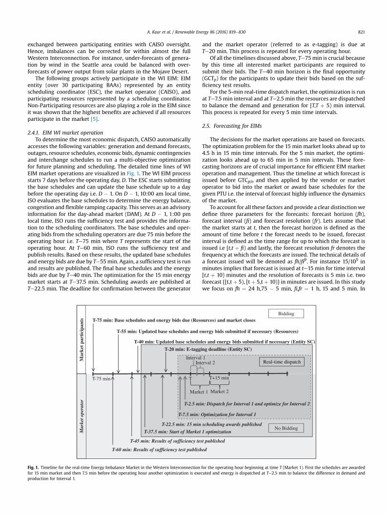
accesses the following variables: generation and demand forecasts,outages, resource schedules, economic bids, dynamic contingenciesand interchange schedules to run a multi-objective optimizationfor future planning and scheduling. The detailed time lines of WIEIM market operations are visualized in Fig. 1. The WI EIM processstarts 7 days before the operating day, D. The ESC starts submittingthe base schedules and can update the base schedule up to a daybefore the operating day i.e. D � 1. On D � 1, 10:00 am local time,ISO evaluates the base schedules to determine the energy balance,congestion and flexible ramping capacity. This serves as an advisoryinformation for the day-ahead market (DAM). At D � 1, 1:00 pmlocal time, ISO runs the sufficiency test and provides the informa-tion to the scheduling coordinators. The base schedules and oper-ating bids from the scheduling operators are due 75 min before theoperating hour i.e. Te75 min where T represents the start of theoperating hour. At Te60 min, ISO runs the sufficiency test andpublish results. Based on these results, the updated base schedulesand energy bids are due by T�55min. Again, a sufficiency test is runand results are published. The final base schedules and the energybids are due by Te40 min. The optimization for the 15 min energymarket starts at Te37.5 min. Scheduling awards are published atTe22.5 min. The deadline for confirmation between the generator

Mar

ket o

pera

tor

Mar

ket

part

icip

ants

Mark

TT-75 min

T-75 min: Base schedules and energy bids due (Reso

T-60 min: Results of sufficiency test publish

T-55 min: Updated base schedules and e

T-45 min: Results of sufficiency tes

T-40 min: Updated base schedu

T-37.5 min: Start of Market

T-22.5 min: 15 min

T-20 min: E-tagg

T-7.5 min:

T-2.5 mi

IntervalInt

Fig. 1. Timeline for the real-time Energy Imbalance Market in the Western Interconnectionfor 15 min market and then 7.5 min before the operating hour another optimization is exeproduction for Interval 1.

and the market operator (referred to as e-tagging) is due atTe20 min. This process is repeated for every operating hour.

Of all the timelines discussed above, Te75min is crucial becauseby this time all interested market participants are required tosubmit their bids. The Te40 min horizon is the final opportunity(GCTp) for the participants to update their bids based on the suf-ficiency test results.

For the 5-min real-time dispatchmarket, the optimization is runat Te7.5 min interval and at Te2.5min the resources are dispatchedto balance the demand and generation for [T,T þ 5) min interval.This process is repeated for every 5 min time intervals.

2.5. Forecasting for EIMs

The decisions for the market operations are based on forecasts.The optimization problem for the 15 min market looks ahead up to4.5 h in 15 min time intervals. For the 5 min market, the optimi-zation looks ahead up to 65 min in 5 min intervals. These fore-casting horizons are of crucial importance for efficient EIM marketoperation and management. Thus the timeline at which forecast isissued before GTCp/o and then applied by the vendor or marketoperator to bid into the market or award base schedules for thegiven PTU i.e. the interval of forecast highly influence the dynamicsof the market.

To account for all these factors and provide a clear distinctionwedefine three parameters for the forecasts: forecast horizon (fh),forecast interval (fi) and forecast resolution (fr). Lets assume thatthe market starts at t, then the forecast horizon is defined as theamount of time before t the forecast needs to be issued, forecastinterval is defined as the time range for up to which the forecast isissued i.e [t,t þ fi) and lastly, the forecast resolution fr denotes thefrequency at which the forecasts are issued. The technical details ofa forecast issued will be denoted as fh/fifr. For instance 15/105 inminutes implies that forecast is issued at te15 min for time interval[t,t þ 10) minutes and the resolution of forecasts is 5 min i.e. twoforecast {[t,t þ 5), [t þ 5,t þ 10)} in minutes are issued. In this studywe focus on fh ¼ 24 h,75 � 5 min, fi,fr ¼ 1 h, 15 and 5 min. In

Real-time dispatchReal-time dispatch

Bidding

No Bidding

et 1 Market 2

T+15 min

urces) and market closes

ed

nergy bids submitted if necessary (Resources)

t published

les and energy bids submitted if necessary (Entity SC)

1 optimization

scheduling awards published

ing deadline (Entity SC)

Optimization for Interval 1

n: Dispatch for Interval 1 and optimize for Interval 2

1erval 2 Real-time dispatch

for the operating hour beginning at time T (Market 1). First the schedules are awardedcuted and energy is dispatched at Te2.5 min to balance the difference in demand and

A. Kaur et al. / Renewable Energy 86 (2016) 819e830822

general, for market application fh � GTCp/o and fi � PTU.To be able to participate in EIM, all the participants are required

to provide their resource and load forecasts to the ISO. Since, EIM isdesigned to balance demand and resource at shorter time scales, inthis study we focus on variable energy resource i.e. solar energythat is likely to play an important role in EIM at high penetrationlevels. A brief review on current state of art of solar forecasting isprovided in the following section.

2.5.1. Solar forecastingDepending on the forecast horizon, different methods are

applied for solar forecasting. For intra-week forecasts, NumericalWeather Prediction (NWP) models are known to generate goodresults. This usually holds true for horizons greater than 4 h. Forintra-day forecasts below 4 h, mostly satellite image based pre-diction methods are used [11]. For intra-hour forecasts, local skyconditions and sky images are utilized along with other availablemeteorological data for the site [12e20]. Furthermore, the forecastmodels with no external inputs are also suggested [21] for solarpower for intra-hour forecasts where information is derived fromthe various characteristics in the time-series. Also, forecast modelsare suggested that selects inputs based on spatial and temporaldistributions [22]. A detailed review on solar forecasting method-ologies can be found in Ref. [23].

3. Data sets

3.1. NWP data

Day-ahead Global Horizontal Irradiance (GHI) forecasts gener-ated at the 00:00 coordinated universal time (UTC) are downloadedfrom National Oceanic and Atmospheric Administration (NOAA)servers for December 2012 to December 2013 and degribed forFolsom, CA. This forecast is generated with the Numerical WeatherPrediction (NWP) based on the North American Model (NAM).Forecast horizons ranging from 9 to 35 h with hourly time-resolution are used. The performance of the NAM model is exten-sively evaluated. A general over-prediction of GHI is well known[24e26]. A reforecasting technique is applied on the GHI time-series forecast to remove the bias and structured errors. To eval-uate the model performance, the data set is divided into threedisjoint data sets: training set (12-20-2012 to 1-15-2013), valida-tion set (1-16-2013 to 1-31-2013) and the test set (2-1-2013 to 12-31-2014). The training set is used to train themodels, the validationset is used for optimization as well as for feature selection for theforecast model. The test set is always kept as an independent set toaccess the model performance and report results.

3.2. Ground data

GHI and Direct Normal Irradiance (DNI) data were collected atFolsom, CA, (located at 38.63�N and 121.14�W) using a rotatingshadow-band radiometer (RSR). A CR1000 data logger fromCampbell Scientific running on a 1 min sampling rate was used tostore the data. The sensor of the RSR is a Licor-200SZ photodiode,periodically shaded to provide diffuse irradiance values. DNI valuesare calculated from GHI and diffuse irradiance values, with a pro-gram embedded in the data logger. Sky imagery was acquired withan off-the-shelf fish-eye lens security camera (Vivotek, modelFE8171V) fixed on a horizontal surface and pointed to the zenith,providing one picture every minute. The total costs for thedeployed instruments are below $10,000 USD. The data sets ofirradiance and sky imagery cover December 2012 to December2013.

3.2.1. Data preprocessingThe collected ground data and sky images are pre-processed to

represent 5 and 15min averages. Irradiance time-series and imagesare time-matched and divided into three disjoint data sets:training, validation and testing set as discussed above. In this case,each data set contains subsets of all available months to capture thefull seasonal variation and various sky conditions.

3.2.2. Feature definitionsUsing the time-series and the sky images, features are calculated

to be used an input for the forecast models. To calculate the fea-tures, the clearness index for GHI and DNI is defined as kt ¼ GHI

GHIcsand kb ¼ DNI

DNIcs. The computed features include entropy, backward

averages, and variability for both kt and kb. Entropy is defined as,

Ei ¼ �Xn

j¼1;pijs0

pijlog2�pij

�; i ¼ ð1;2;…;24Þ (1)

where pij is the relative frequency for the jth bin out of the 200 binsin the range [0,2] for data in the interval [t � id,t] and d ¼ 5 min isthe minimum window size. The index i ranges from 1 to 24, indi-cating the smallest window is 5 min and the largest is 120 min.

Backward averages are defined as,

BiðtÞ ¼1N

Xt2½t�id;t�

ktðtÞ; i ¼ ð1;2;…;24Þ (2)

where N is the number of data points in the interval [t � idt, t].Variability is defined as:

ViðtÞ ¼ffiffiffiffiffiffiffiffiffiffiffiffiffiffiffiffiffiffiffiffiffiffiffiffiffiffiffiffiffiffiffiffiffiffiffiffiffiffi1N

Xt2½t�id;t�

DktðtÞ2vuut ; i ¼ ð1;2;…;24Þ (3)

where Dkt(t) ¼ kt(t) � kt(t � dt).The imagery features include entropy, mean, and standard de-

viation for blue channel, green channel, red channel, red/blue ratio,and normalized red/blue ratio. All imagery features have minimumwindow sizes of 1 min, maximumwindow sizes of 10 min, windowincrements of 1 min, and feature length of 24. More details can befound in Ref. [27].

3.3. Solar power modeling

The PVwatts tool, available from the National Renewable EnergyLaboratory (NREL), is applied to get solar data for 1MW fixed, (openrack) array, commercial solar plant for the same location as theirradiance data sets. The characteristics chosen for the power plantare: array tilt¼ 20�, array azimuth¼ 180�, and system losses¼ 14%.The data provided by this software is hourly data. A model isderived between the solar power produced and GHI to be able towork with a higher temporal resolution.

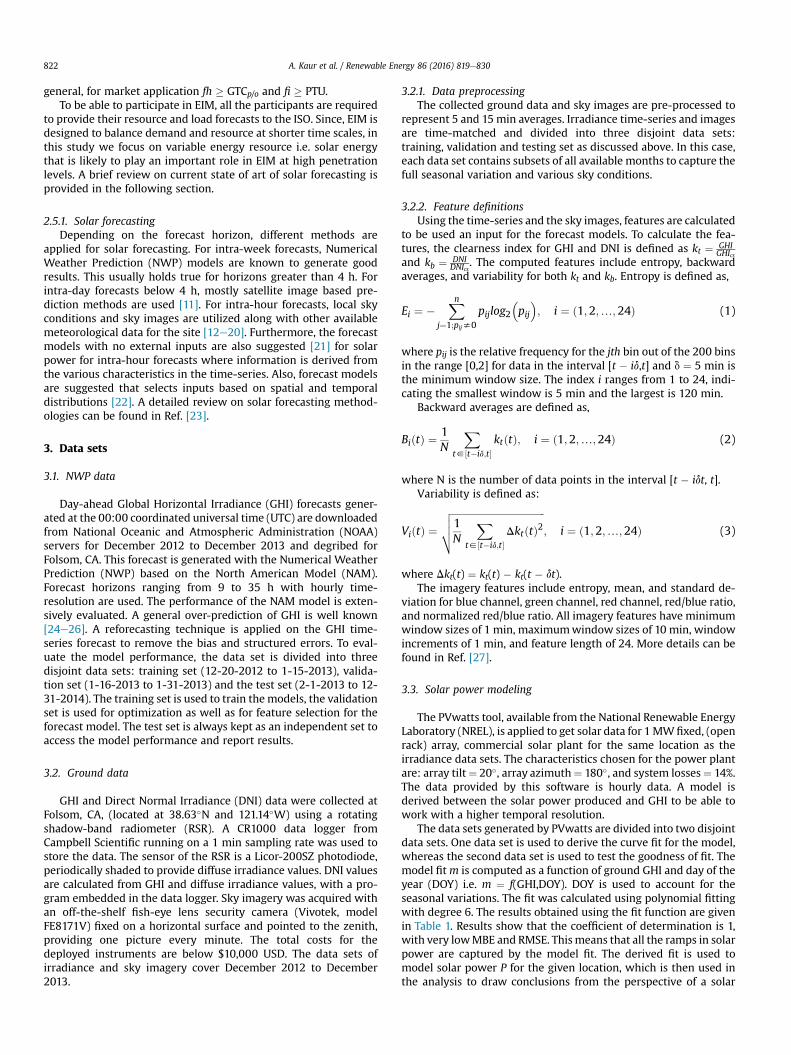
The data sets generated by PVwatts are divided into two disjointdata sets. One data set is used to derive the curve fit for the model,whereas the second data set is used to test the goodness of fit. Themodel fitm is computed as a function of ground GHI and day of theyear (DOY) i.e. m ¼ f(GHI,DOY). DOY is used to account for theseasonal variations. The fit was calculated using polynomial fittingwith degree 6. The results obtained using the fit function are givenin Table 1. Results show that the coefficient of determination is 1,with very lowMBE and RMSE. Thismeans that all the ramps in solarpower are captured by the model fit. The derived fit is used tomodel solar power P for the given location, which is then used inthe analysis to draw conclusions from the perspective of a solar

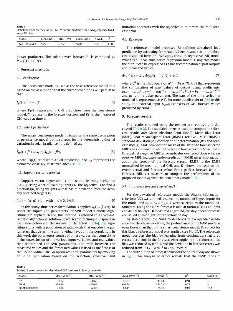
Table 1Statistical error metrics for GHI to PV output modeling for 1 MWp capacity fixed-array PV plant.

Model MAE (kW) MBE (kW) RMSE (kW) rRMSE R2

GHI-PV model 9.27 �0.71 16.81 9.21 1.00

A. Kaur et al. / Renewable Energy 86 (2016) 819e830 823

power producers. The solar power forecast P^ is computed asbP ¼ f ðdGHI;DOYÞ.4. Forecast methods

4.1. Persistence

The persistence model is used as the basic reference model. It isbased on the assumption that the current conditions will persist sothat,

bIpðt þ fhÞ ¼ IðtÞ; (4)

where I p(t) represents a GHI prediction from the persistencemodel, fh represents the forecast horizon, and I(t) is the measuredGHI value at time t.

4.2. Smart persistence

The smart persistence model is based on the same assumptionas persistence model but it corrects for the deterministic diurnalvariation in solar irradiance. It is defined as,

bIspðt þ fhÞ ¼ ktðtÞ�ICSðt þ fhÞ; (5)

where I sp(t) represents a GHI prediction, and ICS represents theestimated clear sky solar irradiance [28e30].

4.3. Support vector regression

Support vector regression is a machine learning technique[31,32]. Using a set of training inputs U, the objective is to find afunction f(u) using weights w that has 2 deviation from the actu-ally obtained targets kt

f ðuÞ ¼ ⟨w;u⟩þ b with w2U; b2ℝ: (6)

In this study, time-series formulation is applied kt(t) ¼ f(u(t)). Toselect the inputs and parameters for SVR model, Genetic Algo-rithms are applied. Hence, this method is referred to as SVR-GA.Genetic algorithm is solution space search technique inspired innatural-selection and the survival of the fittest [33,34]. The algo-rithm starts with a population of individuals that encodes the pa-rameters that determine an individual layout in the population. Inthis work the parameters consist of binary values that control theinclusion/exclusion of the various input variables, and real valuesthat determined the SVR parameters. The MSE between themeasured values and the forecasted values is used as the fitness ofthe GA individual. The GA optimizes these parameters by evolvingan initial population based on the selection, crossover and

Table 2Statistical error metrics for day-ahead GHI forecasts in hourly intervals.

Model MAE (Wm�2) MBE (Wm�2)

SP 37.04 �0.69NAM 109.86 �69.65NAM-Reforecast 31.66 �22.84

mutation operators with the objective to minimize the MSE fore-cast error.

4.4. Reforecast

The reforecast model proposed for refining day-ahead loadprediction by correcting for structured errors and bias in the fore-cast is applied here [35]. We apply the auto-regressive (AR) modelwhich is a linear, time-series regression model. Using this model,the output can be expressed as a linear combination of past outputsand measured values,

AðqÞIrðtÞ ¼ BðqÞINAMðt � nkÞðtÞ þ eðtÞ (7)

where qN is the shift operator, q±N ¼ I(t ± N), A(q) that representsthe combination of past values of output using coefficients,a1,a2,/,ana, A(q) ¼ 1 þ a1q

�1þ/þanaq�na, B(q) ¼ b1þ/þbnbq

�nbþ1

and nk is time delay parameter. The part of the time-series notmodeled is represented as e(t). For more details refer to [36]. In thisstudy, the external input INAM(t) consists of GHI forecast valuespredicted by NAM.

5. Forecast results

The results obtained using the test set are reported and dis-cussed (Table 2). The statistical metrics used to compare the fore-cast results are: Mean Absolute Error (MAE), Mean Bias Error(MBE), Root Mean Square Error (RMSE), relative RMSE (rRMSE),standard deviation (s), coefficient of determination (R2) and fore-cast skill (s). MAE provides the mean of the absolute forecast error,MBE gives information about the bias in forecast error (Measurede

Forecast). A negative MBE error indicates over prediction whereaspositive MBE indicates under-prediction. RMSE gives informationabout the spread of the forecast errors, rRMSE is the RMSEnormalized by mean annual GHI, and R2 shows the relation be-tween actual and forecast value. For a perfect forecast R2 ¼ 1.Forecast skill is a measure to compare the performance of theproposed model against the benchmark model [37].

5.1. Intra-week forecast (day-ahead)

For the day-ahead reforecast model, the Akaike informationcriterion (AIC) was applied to select the number of lagged inputs forthe model and na ¼ nb ¼ nk ¼ 1 were selected as the model pa-rameters. Using the NAM forecast issued at 00:00 UTC as an inputand actual hourly GHI measured at ground, the day-ahead forecastsare issued at midnight for the following day.

As stated above, the NAM model tends to over-predict irradi-ance. For the chosen location, the performance of the NAMmodel iseven lower than that of the smart persistence model. To correct forthis bias, a reforecast model was applied (see Fig. 2). The reforecastmodel corrects the bias by learning from continuous, structurederrors, occurring in the forecast. After applying the reforecast, thebias was reduced by 67.21% and the deviation in forecast errors wasreduced from 151.72 Wm�2 to 78.91 Wm�2.

The distribution of forecast errors for the hours of day are shownin Fig. 3. An analysis of errors reveals that the NWP tends to

RMSE (Wm�2) s (Wm�2) R2 Skill S(%)

96.07 96.08 0.91 e

166.94 151.72 0.72 e

82.14 78.91 0.93 14.5

Fig. 2. Sample day of GHI forecast by NAM and reforecast model. The reforecast model corrects for the bias in the NAM forecast. If ramps are not predicted in NAM, it is unlikely thatthe reforecast model captures them. Both, NAM and reforecast model, tend to over predict. The bottom plot shows the reduction in absolute error. For clear days, the error is close tozero. Most high magnitude errors occur during overcast and cloudy conditions.

A. Kaur et al. / Renewable Energy 86 (2016) 819e830824

overestimated GHI before noon and underestimates the GHI after14:00 PST. After the application of the reforecast model, this bias isreduced. The magnitude of bias in reforecast errors remains un-changed over the day except for sunrise and sunset times. Thisconsistent error can be accounted for duringmarket operations andreserve allocation.

5.2. Intra-hour forecast

The intra-hour forecasts are implemented using a well known,open source machine learning library (LIBSVM) [38]. For intra-hourforecasts, the optimization is performed once for one step aheadprediction. The features and lag of the features selected by the GA

Fig. 3. Mean and standard deviation of day-ahead forecast errors for GHI as a functionof hour of the day. The NAM tends to over-predict until noon and then under-predictslater. The reforecast model corrects for the bias in the forecast and achieves consistentperformance throughout the day.

are given in Table 3. General practice in forecasting is to propagatethe 1 step ahead forecast into the forecast model as an input toforecast the next steps. Doing so, the errors in the forecasts are alsopropagated into next intervals and the forecasts become correlated.To avoid this correlation between various forecasts, the featuresselected by the GA are used to train the models specific for eachforecast horizon and forecast interval. This ensures that eachforecast is independent of each other and they can be studiedindependently. The persistence and smart persistence models areimplemented according to Equations (4) and (5).

5.2.1. 15-minute Interval forecastsThe forecasts in 15 min intervals are produced for forecast ho-

rizon: 15, 30, 45, 60, and 75min. The statistics on the forecast errorsare reported in Table 4. The trend in RMSE and standard deviationof the forecast errors for persistence, smart persistence and state ofart forecast model is shown in Fig. 4. With increasing forecast ho-rizon, the RMSE and standard deviation increases linearly for the Pmodel, whereas in case of SP and SVR-GA, after the forecast horizonof 45 min, the RMSE converges with small change in magnitude.The skill achieved by SVR-GA model, with respect to the P and SPmodels, ranges from 20.26 to 40.86% and 14.53e20.11%respectively.

Table 3Features selected by GA for 15 min and 5 min forecast intervals for the SVR-GAmodel.

15-min Intervals 5-min Intervals

Features Lag Features Lag

GHI, Backward Average 6 GHI, Backward Average 2GHI, Lagged values 3 GHI, Lagged Values 1Image, Blue Average 1 Image, Blue Average 1Images, nRedBlue Entropy 2 Image, RedBlue Entropy 8Image, Red Entropy 1 Image, Red Entropy 1Image, Red Std 3 DNI, Lagged values 1DNI, Backward Average 3 DNI,Variability 1DNI, Lagged Value 3 e e

Table 4Statistical error metrics for short-term solar irradiance forecast in 15 min intervals.

Forecast horizon(min)

Persistence Smart persistence SVR-GA

MAE(Wm�2)

MBE(Wm�2)

RMSE(Wm�2)

rRMSE(�)

MAE(Wm�2)

MBE(Wm�2)

RMSE(Wm�2)

rRMSE(�)

Skill-P(%)

MAE(Wm�2)

MBE(Wm�2)

RMSE(Wm�2)

rRMSE(�)

Skill-P(%)

Skill-SP(%)

15 24.95 1.59 44.17 9.32 15.01 0.35 41.21 8.70 6.70 13.55 0.97 35.22 7.43 20.26 14.5330 36.41 2.41 57.69 12.15 19.36 0.58 51.18 10.78 11.28 16.86 0.54 42.56 8.97 26.22 16.6445 46.63 2.99 68.24 14.36 22.26 0.79 57.20 12.04 16.18 19.01 0.57 46.66 9.82 31.62 18.4260 56.18 3.35 77.61 16.32 24.38 0.99 61.19 12.87 21.16 20.53 0.04 49.25 10.36 36.54 19.5175 65.43 3.50 86.63 18.21 26.06 1.22 64.14 13.48 25.96 21.74 0.04 51.24 10.77 40.85 20.11

Fig. 4. RMSE and standard deviation for short-term GHI forecasts for the 15 minforecast interval with forecast horizon ranging from 15 to 75 min. With increasingforecast horizon, the standard deviation for the P model increases linearly. For the SPand SVR-GA model, the increase in RMSE and standard deviation is very small for the45e75 min forecast horizon.

A. Kaur et al. / Renewable Energy 86 (2016) 819e830 825

5.2.2. 5-minute Interval forecastsThe 5 min interval forecasts are produced up to a forecast ho-

rizon of 5e75 min (see Fig. 5). The error statistics for all the forecasthorizons are provided in Table 5. For the P model, the RMSE errorincreases from 40.43 to 173.61 Wm�2 as the forecast horizon in-creases from 5 to 75 min. The trend in error is linear. In case of SP,there is steep increase in RMSE from 5 to 20min and afterwards theerror magnitude starts converging and the increase in error is only10 Wm�2 as the forecast horizon changes from 25 to 75 min.Similar patterns are observed in the results for SVR-GA. Further-more, the SP always underestimates GHI irrespective of the forecasthorizonwhereas the SVR-GA initially underestimates for 5e25 min

Fig. 5. RMSE and standard deviation for short-term solar forecasts with horizons of 5e75 miincreases linearly. The error is almost constant after a 25 min forecast horizon for the Sma

forecast horizon. Afterwards, it overestimates GHI resulting in anegative bias.

Using P as a reference model, the forecast skill achieved by SPand SVR ranges between 3.41 to 56.21% and 17.86e61.74% respec-tively. Comparing the rRMSE forecast errors to evaluate the per-formance of P and SP for 5e25 min forecast horizon, theimprovements are marginal. As the forecast horizon starts to in-crease, the improvements start increasing linearly. There is clearbenefit in using smart persistence over persistence model and inusing SVR-GA over smart persistence. A skill of 14.49% can be ex-pected using SVR-GA over SP. After a forecast horizon of 40min, theimprovements achieved by the forecast model are not consistent asthe forecast age increases and ground imagery is not sufficientenough to capture cloud dynamics outside this time horizon. Forforecast horizon greater than 40 min, additional data such as sat-ellite imagery can be taken into account if higher accuracy isrequired.

The cumulative frequency distribution (CDF) for the forecasterrors is shown in Fig. 6. Using SP and SVR-GA reduce the spread inthe forecast model. Comparing all the three models, there is0.3e0.6 probability that error will be between ±1% for P, ±0.1% forSP and 0�0.2% for the forecast model. Since positive error meansunderestimation, there is excess of energy as compared to esti-mated. This kind of forecast is beneficial for the market participantas they can curtail extra energy. More details about the value ofthese forecasts for real-time energy imbalance markets is discussednext.

6. Implications on EIMs

6.1. Reserve scheduling

In the United States, all ISOs are required by FERC to keep

n in 5 min intervals. With increasing forecast horizon the error in Persistence (P) modelrt Persistence (SP) and SVR-GA forecast model.

Table 5Statistical error metrics for short-term solar irradiance forecast in 5-min intervals.

Forecast horizon(min)

Persistence Smart persistence SVR-GA

MAE(Wm�2)

MBE(Wm�2)

RMSE(Wm�2)

rRMSE(�)

MAE(Wm�2)

MBE(Wm�2)

RMSE(Wm�2)

rRMSE(�)

Skill-P(%)

MAE(Wm�2)

MBE(Wm�2)

RMSE(Wm�2)

rRMSE(�)

Skill-P(%)

Skill-SP(%)

5 19.81 1.13 40.43 8.54 13.42 0.24 39.05 8.25 3.41 12.62 1.35 33.21 7.02 17.86 14.9510 32.26 2.06 55.52 11.71 18.87 0.47 51.28 10.81 7.64 17.05 0.89 44.33 9.35 20.15 13.5515 42.77 2.75 66.25 13.95 22.17 0.68 58.06 12.22 12.36 19.40 0.83 48.45 10.20 26.87 16.5520 52.58 3.22 75.78 15.94 24.62 0.89 62.74 13.20 17.21 21.44 0.95 52.34 11.01 30.93 16.5725 61.80 3.47 84.41 17.74 26.33 1.10 65.70 13.81 22.17 22.91 0.11 55.33 11.63 34.45 15.7830 70.93 3.52 93.32 19.61 27.96 1.33 68.40 14.38 26.70 24.27 �0.37 57.45 12.08 38.44 16.0135 80.01 3.35 101.71 21.39 29.20 1.56 69.86 14.69 31.31 25.42 �0.50 59.46 12.50 41.14 14.8940 88.80 2.98 110.05 23.16 30.12 1.81 70.74 14.89 35.72 26.21 �0.72 60.37 12.70 45.14 14.6645 97.42 2.38 118.75 25.02 30.87 2.04 71.76 15.12 39.57 26.96 �0.87 61.69 13.00 48.05 14.0350 106.02 1.53 127.38 26.89 31.38 2.23 72.15 15.23 43.36 27.42 �1.47 62.49 13.19 50.94 13.3955 114.97 0.45 136.73 28.93 32.15 2.39 73.48 15.55 46.26 28.08 �0.96 63.53 13.44 53.54 13.5460 123.87 �0.86 146.02 30.98 32.81 2.52 74.48 15.80 48.99 28.43 �0.86 64.50 13.68 55.83 13.4065 132.63 �2.37 155.31 33.06 33.28 2.60 75.30 16.03 51.52 28.99 �0.94 65.07 13.85 58.10 13.5970 141.24 �4.07 164.50 35.14 33.78 2.65 75.66 16.16 54.00 29.22 �0.46 65.19 13.93 61.37 13.8475 149.79 �5.96 173.61 37.23 34.16 2.63 76.03 16.31 56.21 30.97 �0.14 66.42 14.24 61.74 12.64

Fig. 6. Cumulative frequency distribution (CDF) of the solar forecast errors in 5 min intervals for the Persistence (P), Smart persistence (SP) and forecast model (SVR-GA) for theforecast horizon ranging from 5 min to 75 min. The color bar represents the CDF ranging from 0 to 1. The spread of errors in the P model is reduced by the SP and SVR-GA. For the5 min forecast horizon, there is 0.4e0.6 probability that there will be ±1% error whereas with SP it is only ±0.1%. (For interpretation of the references to colour in this figure legend,the reader is referred to the web version of this article.)

A. Kaur et al. / Renewable Energy 86 (2016) 819e830826

additional operating reserves to account for errors and any suddenchanges in load. Reserve requirements also apply for EIMs and thecosts for backup resources effect all market participants. There arevarious methods in practice to compute reserves [39,40,4].

The dominant approach is the n-sigma method, where reservesare calculated by assessing the standard deviation in generationand demand forecast. Based on the forecast above, we can quantifythe required resources necessary to cover the uncertainty intro-duced into the EIM by solar generators with the P, SP and SVR-GAmodels. Fig. 7 shows the standard deviations and respective errorreduction achieved by SP and SVR-GA model for 1 day and 75 to5 min forecast horizons in the intervals of 1 h, 15 min and 5 minaverages. As expected, the standard deviation for 15min averages islower than for 5 min averages. A 15 min market operation disre-gards large shares of variance occurring under 5 min marketoperation, suggesting that lower reserves have to be scheduled.This is counter intuitive but can be explained by the fact thattemporal smoothing disregards large shares of variability (the so-lution is discussed further in Section 6.3). This shows that the dy-namics and operations of the market are highly influenced by the

PTUs and GCTs.Depending on GCT, reserves are scheduled. For GCT >75 min,

required relative reserve are defined. For GCT <75 min, flexibilityreserves are scheduled.

6.2. EIMs with GCT greater than 75 min

The scheduled relative reserve Rr for GCT >75 min is by defini-tion a function of standard deviation of forecast errors s(e) occur-ring for a given PTU, normalized by the mean annual solarirradiance (GHI) received on a given location i.e.,

Rr ¼ sðeÞGHI

: (8)

This approach enables to compare reserve required for differentresource forecast approaches. In practice, the standard deviation ofpower forecast errors is considered (this requires knowledge ofspecific system characteristics). Resource forecasts directly trans-late into power forecasts which validates our use of relative reserve

Fig. 7. Standard deviation in forecast error for forecast horizons ranging from 1 day to 5 min ahead forecast horizons in 1 h, 15 min and 5 min resolution. The total height of the barrepresents the standard deviation in the P forecast errors and then the stacks within a bar shows the reduction in s by the SP and SVR-GA model. For the one day-ahead forecast, thestandard deviation is the highest for the plain NAM forecast, followed by P model. The best performance is achieved by the reforecast model. This chart can be used for any solarforecast application study to design the modeling parameters for the uncertainty at various time-horizons.

A. Kaur et al. / Renewable Energy 86 (2016) 819e830 827

as an estimation for operating reserves. For large GCT, NWP pre-dictions have to be used for the resource forecast. As shown above,reforecasting significantly enhances the performance of NWP basedGHI prediction. Hence, required reserves can be significantlyreduced by the proposed reforecast method (see Section 4.4). Usingthe SPmodel the required reserve is 0.39. Using the NWP reforecastmodel it decreases to 0.32 which is a reduction of 17.84%.

6.3. EIMs with GCT less than 75 min

For markets with GCT � 75 min, the concept of flexibility re-serves allocation is used. Flexibility reserves are scheduled as afunction of change in standard deviation with respect to themagnitude of solar power production [6]. To show the comparisonwith GCT >75 min, relative reserves are also computed.

As discussed above, to account for the problem of temporalsmoothing the resolution of the forecast fr has to be considered i.e.,for a given fr and fi there will be n number of forecasts such thatn ¼ fi

fr. The forecast errors for all these n forecasts are represented asel such that l2{1,2,/,n}. Then, the standard deviation used tocompute the relative reserve has to be greater than or equal to themaximum of standard deviation of el forecast errors,

sðeÞfr � maxlðsðelÞÞ; (9)

where s(e)fr is the standard deviation in n forecast errors occurringin a given PTU with a forecast resolution fr. For example, if themarket operates on PTU ¼ 15 min, and the reserves allocated needto cover the variance up to 5 min time resolution, then n ¼ 3. Fig. 8shows the relative reserves allocation for various forecast-horizonsin 5 and 15 min intervals, considering the 5 min variance. Thereduction of reserve required using P model compared to SP andSVR-GA is shown. The grey-scale bar represents the reserve allo-cation for 15 min interval. Colored bars represent the reserveallocation for the 5 min time interval. It is beneficial for the marketoperator to allocate resources on shorter time horizons. For short-term forecast horizon (5e15 min), the reduction is smaller whereasfor the higher forecast horizons, the benefits of using SP and fore-cast model become apparent. The relative reserved can be reducedby 28.5% on average. For 45 min forecast horizon, the relativereserve required is 0.25 and it can be reduced by 40% using the SPmodel.

6.3.1. Market operator e schedulersThe computed flexibility reserves are shown in Fig. 9). The

reduction of flexibility reserves using the P model, compared to SPand SVR-GA are summarized in Table 6. Using the SP model theimprovement ranges between 5.83% and 59.97% for the 5e75 minforecast horizon, respectively. The reductions using SVR-GA rangesbetween 22.62% and 67.47%, respectively. Using SVR-GA instead ofSP, the flexibility reserves can be reduced by 21%, on average.However, reductions are lower for the 15 min forecast intervals.This is expected because at 15 min resolution the resource vari-ability is lower than for 5 min.

6.3.2. Market participant e power generatorsThe technical requirements of the power grid depend upon very

small discrepancies between generation and load. This drives theneed for imbalance settlements. For intermittent renewable gen-erators, FERC defines errors in market bids larger than 7.5% as abenchmark for penalties. Hence, we define errors larger than 7.5%as occurring imbalance. To quantify the likelihood that imbalanceswill occur, the probability of wrong bids through errors in forecastsfor 5 min intervals for a 1 MW solar plant are calculated. For5e75 min forecast, the probability ranges between 0.15 and 0.41,0.08 to 0.17, and 0.07 to 0.14 for persistence, smart persistence andforecast model, respectively (see Fig. 10). Thus, the probability ofimbalance can be reduced by 66.93% using SVR-GA instead of P (or19.65% instead of SP model). Similar results are achieved for the15 min forecast resolution, where the probability of an imbalance isreduced by 15.12% by replacing SP with SVR-GA.

6.4. Implications for the Western Interconnection EIM

Most imbalance markets around the world are operated at15 min or greater PTU, however the Energy Imbalance Market inthe Western Interconnection is a unique platform where after a15 min market, another 5 min market is operated. This sectionpresent results with respect to the timescales for Western Inter-connection from the perspective of both, the market operator andmarket participants.

Let assume the market operator starts the optimization toexecute the WI EIM at Te37.5 min to plan for the interval [T,T þ 15)using the state-of-the-art forecast issued at Te45 min. Then, in thistime interval the forecast error lies between�0.8 and 0.09 kWm�2

Fig. 8. Benefits of 5 min versus 15 min reserve allocation for real-time markets considering 5 min data interval. The grey-scale bar plots shows the relative reserve required for the15 min-time intervals whereas the colored bar represents the reserves required for the 5 min time-intervals. The total height of the bar represents the total reserve required usingthe persistence model and reduction in the magnitude of reserves is shown by the stacks within each bar. (For interpretation of the references to colour in this figure legend, thereader is referred to the web version of this article.)

Fig. 9. Flexibility reserve required for 1 MW solar plant for 5 min intervals. The total magnitude of the bar represents the flexibility reserve needed using the Persistence model andthe inner stack represents the magnitude reduction by Smart persistence and the forecast model. Beginning from forecast horizon of 5 mine55 min, the improvements in reducingflexibility reserves increase and for the forecast horizons greater than 55 min, the improvements starts decreasing due to reduced forecast skill.

A. Kaur et al. / Renewable Energy 86 (2016) 819e830828

for a 90% confidence interval. Therefore, if another state-of-the artforecast for a forecast horizon of Te10 min is added to the systembefore the optimization runs for Te7.5 min, the uncertainity ofover-prediction can be reduced from �0.6 to 0.04 kWm�2, repre-senting a 25% reduction and 41% overall reduction of variance (seeFig. 11).

For WI EIM participation, market participants are mandated tosubmit a bid at Te75 min for the [T,Tþ 15 min) time-interval. Usinga forecast model instead of SP model, the chances of gettingpenalized reduces by 15.65%. Furthermore, if the bid is updatedTe45 min, there is a 13.11% reduction in chances of getting penal-ized using SVR-GA as compared to the SP model.

7. Conclusions

A review about energy imbalance markets is presented. The keydesign variables are explained and their significance is discussed. It

is shown that the program time unit as well as the gate closure timeare the key variables controlling the market dynamics. The processof imbalance settlements are the key regulatory and economicaldrivers for market participants and the operator.

The benefits of solar resource and power forecasting are quan-tified in terms of reduction of required backup resources and theoccurrence of energy imbalances. This analysis is based on day-ahead and short-term solar resource forecasts covering forecasthorizons ranging from 1 day to 5 min in 1 h, 15 and 5 min intervals.State-of-the-art forecasts (with reforecast enhancements) areshown. The reforecast methodology reduces the bias in day-aheadforecast by 67.21% in NAM forecast and achieves a forecast skill of14.5% over the smart persistence model. The error of the persis-tence model increases linearly, whereas smart persistence and theSVR-GA model, the error converges by forecast horizon of 25 minfor 5 min resolution. The skill achieved by SVR-GA ranges between14.53e20.11% and 12.64e16.75% for 15 min and 5 min forecast

Table 6Summary of benefits of solar forecasting for the real-time energy markets with respect to the Persistence (P) and Smart persistence (SP) forecast model using solar power datafor 1 MW plant.

Forecast horizon (min) Reduction w.r.t. P model [%] Reduction w.r.t. SP model [%]

Flexibility reserve p(Error > 7.5%) FR p(Error > 7.5%)

SP SVR-GA SP SVR-GA SVR-GA SVR-GA

fr�5 min5 5.83 22.62 44.38 53.04 17.83 15.6410 11.23 26.41 53.66 62.40 17.11 18.8515 16.99 33.89 59.32 66.03 20.36 16.4820 22.18 39.76 62.01 68.20 22.59 16.3025 27.65 41.93 63.43 69.06 19.73 15.3830 31.80 46.63 63.47 69.80 21.74 17.3235 35.51 50.02 63.19 69.91 22.49 18.2540 39.31 54.70 62.35 70.20 25.36 20.8545 42.89 56.01 60.79 70.55 22.97 24.8950 46.49 57.69 59.51 68.89 20.94 24.8255 49.24 60.10 59.26 68.89 21.40 25.6460 52.69 63.43 58.65 67.88 22.71 23.3265 56.27 65.16 58.02 67.32 20.32 22.1570 58.19 67.16 57.62 66.39 21.45 20.6875 59.97 67.47 57.47 64.45 18.75 16.41

fr�15 min15 10.20 22.29 50.02 59.30 13.47 18.5730 15.72 29.27 57.43 63.38 16.09 13.9645 20.91 36.32 61.16 66.25 19.48 13.1160 26.19 42.67 63.12 68.42 22.34 14.3375 30.99 47.19 63.72 69.40 23.48 15.65

Fig. 10. Energy imbalances (probability for the error to exceed 7.5%) for 1 MW solarplant for 5e75 min and 15e75 min forecast horizon with 5 min and 15 min resolution.The probability of imbalance greater than 7.5% can be reduced by an average of 19.65%and 15.12% by using a forecast model instead of a SP model.

Fig. 11. Inverse cumulative frequency distribution of the expected forecast errors thatmarket operator has to optimize for in 5-min market after scheduling the awards for15 min market using the forecast model. Results show that if a forecast model isapplied at 10 min forecast horizon in 5 min resolution the uncertainty can be reducedfrom �0.08 to �0.06 kW m�2 and from 0.09 to 0.04 kWm�2 for 90% of the time.

A. Kaur et al. / Renewable Energy 86 (2016) 819e830 829

intervals (forecast horizons ranging from 5 to 75min). For forecasts,covering greater than or equal to 35 min forecast horizons, the skilldrops implying that more sophisticated methods e.g. includingsatellite imagery are required in addition to ground data.

The application of the discussed forecasts reduce the relativereserve requirement for participation in imbalance markets withday-ahead gate closure time by 17.84%. Similarly for EIMs withshorter gate closure time, the flexibility reserves for an explanatory1 MW solar plant can be reduced by 21% on average, for the 5 minforecast-intervals. For 15 min forecasts, the improvements are16.14% compared to the smart persistence model. The improve-ments for the 15-min intervals are smaller than for 5 min intervalsdue to variability smoothing. For participating commercial solar

producers, the probability of causing an imbalance is reduced by19.65% and 15.12% for 5 min and 15 min forecast intervals. Theimprovements achieved through forecasting depend on marketoperation time scales. Having the flexibility to operate on shorttime-horizons reduces reserve requirements and the probabilitiesof occurring imbalance settlements.

Acknowledgements

Partial funding for this research was provided by the CaliforniaPublic Utilities Commission under the California Solar InitiativePrograms CSI 3 and 4. Partial funding from San Diego Gas& Electricis also gratefully acknowledged.

References

[1] L. Bird, M. Milligan, D. Lew, Integrating Variable Renewable Energy: Chal-lenges and Solutions, Tech. Rep., Technical Report, National Renewable EnergyLaboratory, 2013. September, accessible at: http://www.nrel.gov/docs/fy13osti/60451.pdf.

[2] A. Mills, A. Botterud, J. Wu, Z. Zhou, B. M. Hodge, M. Heaney, Integrating Solar

A. Kaur et al. / Renewable Energy 86 (2016) 819e830830

pv in Utility System Operations, Tech. Rep. ANL/DIS-13/18.[3] Q. Wang, C. Zhang, Y. Ding, G. Xydis, J. Wang, J. Østergaard, Review of real-

time electricity markets for integrating distributed energy resources and de-mand response, Appl. Energy 138 (2015) 695e706.

[4] R. Orans, A. Olson, J. Moore, J. Hargreaves, R. Jones, G. Kwok, F. Kahrl, C. Woo,Energy imbalance market benefits in the west: a case study of pacificorp andCAISO, Electr. J. 26 (5) (2013) 26e36.

[5] J. King, B. Kirby, M. Milligan, S. Beuning, Flexibility Reserve Reductions from anEnergy Imbalance Market with High Levels of Wind Energy in the WesternInterconnection, Tech. rep., National Renewable Energy Laboratory (NREL),Golden, CO, 2011.

[6] M. Milligan, K. Clark, J. King, B. Kirby, T. Guo, G. Liu, Examination of PotentialBenefits of an Energy Imbalance Market in the Western Interconnection, 2013.Tech. Rep. TP-5500e57115, NREL.

[7] R.A. van der Veen, R.A. Hakvoort, Balance responsibility and imbalance set-tlement in northern european e an evaluation, in: Energy Market, 2009. EEM2009. 6th International Conference on the European, IEEE, 2009, pp. 1e6.

[8] E. Bitar, R. Rajagopal, P. Khargonekar, K. Poolla, P. Varaiya, Bringing windenergy to market, Power Syst. IEEE Trans. 27 (3) (2012) 1225e1235.

[9] B.M. Hodge, A. Florita, J. Sharp, M. Margulis, D. Macreavy, The Value ofImproved Short-term Wind Power Forecasting, 2015. Tech. rep., NREL.

[10] A. Cifor, P. Denholm, E. Ela, B.M. Hodge, A. Reed, The policy and institutionalchallenges of grid integration of renewable energy in the western UnitedStates, Util. Policy 33 (2015) 34e41.

[11] L. Nonnenmacher, C.F.M. Coimbra, Streamline-based method for intra-daysolar forecasting through remote sensing, Sol. Energy 108 (2014) 447e459.

[12] R. Marquez, C.F.M. Coimbra, Forecasting of global and direct solar irradianceusing stochastic learning methods, ground experiments and the NWS data-base, Sol. Energy 85 (5) (2011) 746e756.

[13] R. Marquez, H.T.C. Pedro, C.F.M. Coimbra, Hybrid solar forecasting methoduses satellite imaging and ground telemetry as inputs to ANNs, Sol. Energy 92(2013) 176e188.

[14] R. Marquez, C.F.M. Coimbra, Intra-hour DNI forecasting based on cloudtracking image analysis, Sol. Energy 91 (2013) 327e336.

[15] R. Marquez, V.G. Gueorguiev, C.F.M. Coimbra, Forecasting of global horizontalirradiance using sky cover indices, J. Sol. Energy Eng. 135 (1) (2012),011017e011017.

[16] Y. Chu, H.T.C. Pedro, C.F.M. Coimbra, Hybrid intra-hour DNI forecasts with skyimage processing enhanced by stochastic learning, Sol. Energy 98 (2013)592e603.

[17] Y. Chu, H.T.C. Pedro, L. Nonnenmacher, R.H. Inman, Z. Liao, C.F.M. Coimbra,A smart image-based cloud detection system for intra-hour solar irradianceforecasts, J. Atmos. Ocean. Technol. 31 (2014) 1995e2007.

[18] Y. Chu, B. Urquhart, S.M.I. Gohari, H.T.C. Pedro, J. Kleissl, C.F.M. Coimbra, Short-term reforecasting of power output from a 48 mwe solar pv plant, Sol. Energy112 (2015) 68e77.

[19] B. Akyurek, A. Akyurek, J. Kleissl, T. Rosing, Tesla: Taylor expanded solaranalog forecasting, in: 2014 IEEE International Conference on Smart GridCommunications (SmartGridComm), 2014, pp. 127e132.

[20] D. Bernecker, C. Riess, E. Angelopoulou, J. Hornegger, Continuous short-termirradiance forecasts using sky images, Sol. Energy 110 (2014) 303e315.

[21] H.T.C. Pedro, C.F.M. Coimbra, Assessment of forecasting techniques for solarpower production with no exogenous inputs, Sol. Energy 86 (7) (2012)2017e2028.

[22] A. Zagouras, H.T.C. Pedro, C.F.M. Coimbra, On the role of lagged exogenous

variables and spatio-temporal correlations in improving the accuracy of solarforecasting methods, Renew. Energy 78 (2015) 203e218.

[23] R.H. Inman, H.T.C. Pedro, C.F.M. Coimbra, Solar forecasting methods forrenewable energy integration, Prog. Energy Combust. Sci. 39 (6) (2013)535e576.

[24] R. Perez, E. Lorenz, S. Pelland, M. Beauharnois, G.V. Knowe, K.H. Jr.,D. Heinemann, J. Remund, S.C. Müller, W. Traunmüller, G. Steinmauer,D. Pozo, J.A. Ruiz-Arias, V. Lara-Fanego, L. Ramirez-Santigosa, M. Gaston-Romero, L.M. Pomares, Comparison of numerical weather prediction solarirradiance forecasts in the US, Canada and Europe, Sol. Energy 94 (2013)305e326.

[25] P. Mathiesen, J. Kleissl, Evaluation of numerical weather prediction for intra-day solar forecasting in the continental united states, Sol. Energy 85 (5) (2011)967e977.

[26] L. Nonnenmacher, A. Kaur, C.F.M. Coimbra, Verification of the SUNY directnormal irradiance model with ground measurements, Sol. Energy 99 (2014)246e258.

[27] H.T.C. Pedro, C.F.M. Coimbra, Nearest-neighbor methodology for prediction ofintra-hour global horizontal and direct normal irradiances, Renew. Energy 80(2015) 770e782.

[28] P. Ineichen, Comparison of eight clear sky broadband models against 16 in-dependent data banks, Sol. Energy 80 (4) (2006) 468e478.

[29] P. Ineichen, R. Perez, A new airmass independent formulation for the Linketurbidity coefficient, Sol. Energy 73 (3) (2002) 151e157.

[30] C. Gueymard, Clear-sky irradiance predictions for solar resource mapping andlarge-scale applications: improved validation methodology and detailedperformance analysis of 18 broadband radiative models, Sol. Energy 86 (8)(2012) 2145e2169.

[31] V. Vapnik, S.E. Golowich, A. Smola, Support Vector Method for FunctionApproximation, Regression Estimation, and Signal Processing, in: Advances inNeural Information Processing Systems, 1997, pp. 281e287.

[32] A.J. Smola, B. Scholkopf, A tutorial on support vector regression, Stat. Comput.14 (3) (2004) 199e222.

[33] J.H. Holland, Adaptation in Natural and Artificial Systems: an IntroductoryAnalysis with Applications to Biology, Control, and Artificial Intelligence, UMichigan Press, 1975.

[34] P. Castillo, J. Merelo, A. Prieto, V. Rivas, G. Romero, G-prop: global optimiza-tion of multilayer perceptrons using gas, Neurocomputing 35 (1) (2000)149e163.

[35] A. Kaur, H.T.C. Pedro, C.F.M. Coimbra, Ensemble re-forecasting methods forenhanced power load prediction, Energy Convers. Manag. 80 (2014) 582e590.

[36] L. Ljung, System Identification: Theory for the User, Prentice Hall PTR, NewJersey, USA, 1999. ISBN 0-13-881640-9 025.

[37] R. Marquez, C.F.M. Coimbra, Proposed metric for evaluation of solar fore-casting models, ASME J. Sol. Energy Eng. 135 (2013) 0110161e0110169.

[38] C.C. Chang, C.J. Lin, LIBSVM: a library for support vector machines, ACM Trans.Intell. Syst. Technol. 2 (2011) software available at: http://www.csie.ntu.edu.tw/~cjlin/libsvm, 27:1e27:27.

[39] H. Holttinen, M. Milligan, E. Ela, N. Menemenlis, J. Dobschinski, B. Rawn,R. Bessa, D. Flynn, E. Gomez Lazaro, N. Detlefsen, Methodologies to determineoperating reserves due to increased wind power, in: 2013 IEEE Power andEnergy Society General Meeting (PES), 2013, pp. 1e10.

[40] B. Mauch, J. Apt, P.M.S. Carvalho, P. Jaramillo, What day-ahead reserves areneeded in electric grids with high levels of wind power? Environ. Res. Lett. 8(3) (2013) 034013.