benford’s law and continuous dependent …€™s law and continuous dependent random variables...

BENFORD’S LAW AND CONTINUOUS DEPENDENT RANDOM VARIABLES

THEALEXA BECKER, DAVID BURT, TAYLOR C. CORCORAN, ALEC GREAVES-TUNNELL, JOSEPH R. IAFRATE,JOY JING, STEVEN J. MILLER, JACLYN D. PORFILIO, RYAN RONAN, JIRAPAT SAMRANVEDHYA,

FREDERICK W. STRAUCH, AND BLAINE TALBUT

Abstract. Many mathematical, man-made and natural systems exhibit a leading-digit bias, where a firstdigit (base 10) of 1 occurs not 11% of the time, as one would expect if all digits were equally likely, but rather30%. This phenomenon is known as Benford’s Law. Analyzing which datasets adhere to Benford’s Law andhow quickly Benford behavior sets in are the two most important problems in the field. Most previous workstudied systems of independent random variables, and relied on the independence in their analyses.

Inspired by natural processes such as particle decay, we study the dependent random variables that emergefrom models of decomposition of conserved quantities. We prove that in many instances the distribution oflengths of the resulting pieces converges to Benford behavior as the number of divisions grow, and giveseveral conjectures for other fragmentation processes. The main difficulty is that the resulting randomvariables are dependent. We handle this by using tools from Fourier analysis and irrationality exponents toobtain quantified convergence rates as well as introducing and developing techniques to measure and controlthe dependencies. The construction of these tools is one of the major motivations of this work, as ourapproach can be applied to many other dependent systems. As an example, we show that the n! entries inthe determinant expansions of n× n matrices with entries independently drawn from nice random variablesconverges to Benford’s Law.

Contents

1. Introduction 21.1. Background 21.2. 1-Dimensional Decomposition Models and Notation 31.3. Results 51.4. Sketch of Proofs 82. Proof of Theorem 1.5: Unrestricted Decomposition 82.1. Expected Value 92.2. Variance 103. Proof of Theorem 1.7: Discrete Decomposition 124. Proof of Theorem 1.9: Restricted 1-Dimensional Decomposition 145. Proof of Theorem 1.11: Fixed 1-Dimensional Proportion Decomposition 155.1. Case I: y ∈ Q. 155.2. Case II: y /∈ Q has finite irrationality exponent 175.3. Case III: y /∈ Q has infinite irrationality exponent 216. Two-Dimensional Fragmentation 216.1. Decomposition of Triangles 216.2. Decomposition of Quadrilaterals 217. Proof of Theorem 1.17: Determinant Expansion 24

Date: July 23, 2017.2010 Mathematics Subject Classification. 60A10, 11K06 (primary), (secondary) 60E10.Key words and phrases. Benford’s Law, Fourier transform, Mellin transform, dependent random variables, fragmentation.This work was supported by NSF grants DMS0850577, DMS0970067, DMS1265673, DMS1561945 and PHY1005571, a

Research Corporation Cottrell College Science Award, and Williams College. We thank Don Lemons, Charles Wohl, andparticipants of numerous Williams SMALL REUs for helpful discussions. This paper is dedicated to the memory of CoreyManack, a wonderful colleague who was generous with his time and provided many helpful comments in the course of theseinvestigations.

1

2 BECKER ET. AL.

8. Future Work 25Appendix A. Non-Benford Behavior 27Appendix B. Notes on Lemons’ Work 29References 29

1. Introduction

1.1. Background. In 1881, American astronomer Simon Newcomb [New] noticed that the earlier pagesof logarithm tables, those which corresponded to numbers with leading digit 1, were more worn than otherpages. He proposed that the leading digits of certain systems are logarithmically, rather than uniformly,distributed. In 1938, Newcomb’s leading digit phenomenon was popularized by physicist Frank Benford,who examined the distribution of leading digits in datasets ranging from street addresses to molecularweights. The digit bias investigated by these scientists is now known as Benford’s Law.

Formally, a dataset is said to follow Benford’s Law base B if the probability of observing a leading digitd base B is logB(

d+1d ); thus we would have a leading digit of 1 base 10 approximately 30% of the time, and

a leading digit of 9 less than 5% of the time. More generally, we can consider all the digits of the absolutevalue of a number. Specifically, given any x > 0 we can write it as

x = SB(x) · 10kB(x), (1.1)

where SB(x) ∈ [1, B) is the significand of x and kB(x) is an integer; note two numbers have the same leadingdigits if their significands agree. Benford’s Law is now the statement that Prob(SB(x) ≤ s) = logB(s).

Benford’s Law arises in applied mathematics [BH1], auditing [DrNi, MN3, Nig1, Nig2, Nig3, NigMi],biology [CLTF, MorSSZ], computer science [Knu], dynamical systems [Ber1, Ber2, BBH, BHKR, Rod],economics [To, V-BFJ], geology [NM], number theory [ARS, KonMi, LS], physics and astrophysics [Buc,El, MorSPZ, NiRen, NiWeRe, PTTV, ShaMa1, ShaMa2], signal processing [PHA], statistics [MN2, CLM]and voting fraud detection [Meb], to name just a few. See [BH2, Hu] for extensive bibliographies and[BH3, BH4, BH5, BH6, Dia, Hi1, Hi2, JKKKM, JR, MN1, Pin, Rai] for general surveys and explanationsof the Law’s prevalence, as well as the book edited by Miller [Mil], which develops much of the theory anddiscusses at great length applications in many fields.

One of the most important questions in the subject, as well as one of the hardest, is to determine whichprocesses lead to Benford behavior. Many researchers [Adh, AS, Bh, JKKKM, Lev1, Lev2, MN1, Rob, Sa,Sc1, Sc2, Sc3, ST] observed that sums, products and in general arithmetic operations on random variablesoften lead to a new random variable whose behavior is closer to satisfying Benford’s law than the inputs,though this is not always true (see [BH5]). Many of the proofs use techniques from measure theory andFourier analysis, and in some special cases it is possible to obtain closed form expressions for the densitieswhich can be analyzed directly. In certain circumstances these results can be interpreted through the lensof a central limit theorem law; as we only care about the logarithms modulo 1, the Benfordness followsfrom convergence of this associated density to the uniform distribution (see for example [MN1] or Chapter3 of [Mil]).

A crucial input in many of the above papers is that the random variables are independent. In this paperwe explore situations where there are dependencies. The dependencies we investigate are different thanmany others in the literature. For example, previous work studied dynamical systems and iterates or powersof a given random variable, where once the initial seed is chosen the resulting process is deterministic; seefor example [AS, BBH, Dia, KonMi, LS]. In our systems instead of having just one random variable wehave a large number of independent random variables N generating an enormous number of dependentrandom variables M (often M = 2N , though in one of our examples involving matrices we have M = N !).This work is the compilation of many projects over the past several years of efforts to build a countingapproach to control the dependencies. To show the utility of this new perspective we successfully apply itin many systems.

Our introduction to the subject of this paper came from reading an article of Lemons [Lem] (though seethe next subsection for other related problems), who studied the decomposition of a conserved quantity;

BENFORD’S LAW AND CONTINUOUS DEPENDENT RANDOM VARIABLES 3

for example, what happens during certain types of particle decay. As the sum of the piece sizes must equalthe original length, the resulting summands are clearly dependent. While it is straightforward to showwhether or not individual pieces are Benford, the difficulty is in handling all the pieces simultaneously. Wecomment in greater detail about Lemons’ work in Appendix B.

In the next subsection we describe some of the systems we study. In analyzing these problems we developa technique to handle certain dependencies among random variables, which we then show is applicable inother systems as well.

1.2. 1-Dimensional Decomposition Models and Notation. The techniques we develop to show Ben-ford behavior for problems with dependent random variables are applicable to many systems. In the interestof space, we will describe in detail here just three variations of a stick decomposition, and later discussconjectures about other possible decomposition processes and some results in higher dimensions. As anexample of the power of this approach we also prove that the leading digits of the n! terms in the determi-nant expansion of a matrix whose entries are independent, identically distributed ‘nice’ random variablesfollow a Benford distribution as n tends to infinity.

There is an extensive literature on decomposition problems; we briefly comment on some other systemsthat have been successfully analyzed and place our work in context. Kakutani [Ka] considered the followingdeterministic process. Let Q0 = {0, 1} and given Qk = {x0 = 0, x1, . . . , xk = 1} (where the xi’s are inincreasing order) and an α ∈ (0, 1), construct Qk+1 by adding points xi + α(xi+1 − xi) in each subinterval[xi, xi+1] where xi+1 − xi = max1≤ℓ≤k−1 |xℓ+1 − xℓ|. He proved that as k → ∞, the points of Qk becomeuniformly distributed, which implies that this process is non-Benford. This process has been generalized;see for example [AF, Ca, Lo, PvZ, Sl, vZ] and the references therein, and especially the book [Bert]. Seealso [Kol] for processes related to particle decomposition, [CaVo, Ol] for 2-dimensional examples, [IV] for afractal setting, and [IMS] for some results on discrete fragmentation also inspired by Lemons’ work.

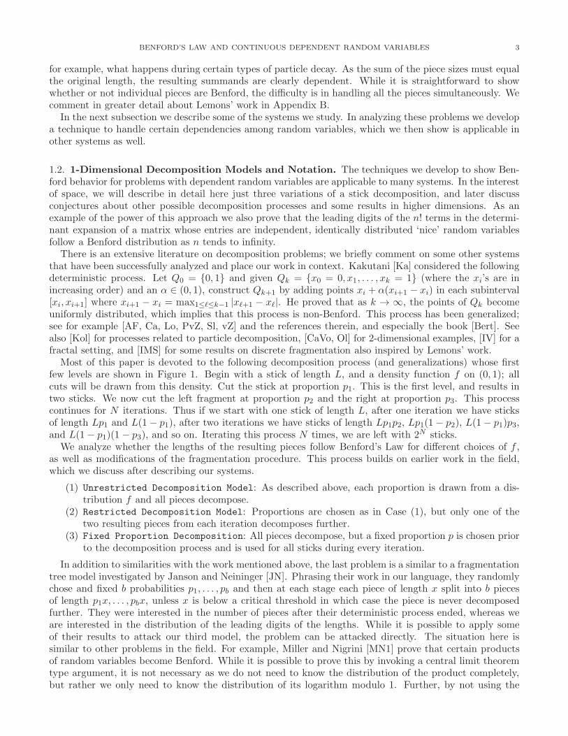
Most of this paper is devoted to the following decomposition process (and generalizations) whose firstfew levels are shown in Figure 1. Begin with a stick of length L, and a density function f on (0, 1); allcuts will be drawn from this density. Cut the stick at proportion p1. This is the first level, and results intwo sticks. We now cut the left fragment at proportion p2 and the right at proportion p3. This processcontinues for N iterations. Thus if we start with one stick of length L, after one iteration we have sticksof length Lp1 and L(1− p1), after two iterations we have sticks of length Lp1p2, Lp1(1− p2), L(1− p1)p3,and L(1− p1)(1 − p3), and so on. Iterating this process N times, we are left with 2N sticks.

We analyze whether the lengths of the resulting pieces follow Benford’s Law for different choices of f ,as well as modifications of the fragmentation procedure. This process builds on earlier work in the field,which we discuss after describing our systems.

(1) Unrestricted Decomposition Model: As described above, each proportion is drawn from a dis-tribution f and all pieces decompose.

(2) Restricted Decomposition Model: Proportions are chosen as in Case (1), but only one of thetwo resulting pieces from each iteration decomposes further.

(3) Fixed Proportion Decomposition: All pieces decompose, but a fixed proportion p is chosen priorto the decomposition process and is used for all sticks during every iteration.

In addition to similarities with the work mentioned above, the last problem is a similar to a fragmentationtree model investigated by Janson and Neininger [JN]. Phrasing their work in our language, they randomlychose and fixed b probabilities p1, . . . , pb and then at each stage each piece of length x split into b piecesof length p1x, . . . , pbx, unless x is below a critical threshold in which case the piece is never decomposedfurther. They were interested in the number of pieces after their deterministic process ended, whereas weare interested in the distribution of the leading digits of the lengths. While it is possible to apply someof their results to attack our third model, the problem can be attacked directly. The situation here issimilar to other problems in the field. For example, Miller and Nigrini [MN1] prove that certain productsof random variables become Benford. While it is possible to prove this by invoking a central limit theoremtype argument, it is not necessary as we do not need to know the distribution of the product completely,but rather we only need to know the distribution of its logarithm modulo 1. Further, by not using the

4 BECKER ET. AL.

L

L K1 LH1-K1L

L K1K2 L K1H1-K2L LH1-K1LK3 LH1-K1LH1-K3L

L K1K2K4 L K1K2H1-K4L L K1H1-K2LK5 L K1H1-K2LH1-K45L LH1-K1LK3K6 LH1-K1LK3H1-K6L LH1-K1LH1-K3LK7 LH1-K1LH1-K3LH1-K7L

Figure 1. Unrestricted Decomposition: Breaking L into pieces, N = 3.

central limit theorem they are able to handle more general distributions; in particular, they can handlerandom variables with infinite variance.

Before we can state our results, we first introduce some notation which is needed to determine which flead to Benford behavior.

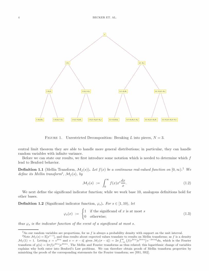
Definition 1.1 (Mellin Transform, Mf (s)). Let f(x) be a continuous real-valued function on [0,∞).1 Wedefine its Mellin transform2, Mf (s), by

Mf (s) :=

∫ ∞

0f(x)xs

dx

x. (1.2)

We next define the significand indicator function; while we work base 10, analogous definitions hold forother bases.

Definition 1.2 (Significand indicator function, ϕs). For s ∈ [1, 10), let

ϕs(x) :=

{1 if the significand of x is at most s

0 otherwise;(1.3)

thus ϕs is the indicator function of the event of a significand at most s.

1As our random variables are proportions, for us f is always a probability density with support on the unit interval.2Note Mf (s) = E[xs−1], and thus results about expected values translate to results on Mellin transforms; as f is a density

Mf (1) = 1. Letting x = e2πu and s = σ − iξ gives Mf (σ − iξ) = 2π∫∞

−∞

(

f(e2πu)e2πσu)

e−2πiuξdu, which is the Fourier

transform of g(u) = 2πf(e2πu)e2πσu. The Mellin and Fourier transforms as thus related; this logarithmic change of variablesexplains why both enter into Benford’s Law problems. We can therefore obtain proofs of Mellin transform properties bymimicking the proofs of the corresponding statements for the Fourier transform; see [SS1, SS2].


In all proofs, we label the set of stick lengths resulting from the decomposition process by {Xi}. Notethat a given stick length can occur multiple times, so each element of the set {Xi} has associated to it afrequency.

Definition 1.3 (Stick length proportions, PN ). Given stick lengths {Xi}, the proportion whose significandis at most s, PN (s), is

PN (s) :=

∑iϕs(Xi)

#{Xi}. (1.4)

In the Fixed Proportion Decomposition Model, we are able to quantify the rate of convergence iflog10

1−pp has finite irrationality exponent.

Definition 1.4 (Irrationality exponent). A number α has irrationality exponent κ if κ is the supremum ofall γ with

limq→∞qγ+1 minp

∣∣∣∣α− p

q

∣∣∣∣ = 0. (1.5)

By Roth’s theorem, every algebraic irrational has irrationality exponent 1. See for example [HS, MT-B,Ro] for more details.

Finally, we occasionally use big-Oh and little-oh notation. We write f(x) = O(g(x)) (or equivalentlyf(x) ≪ g(x)) if there exists an x0 and a C > 0 such that, for all x ≥ x0, |f(x)| ≤ Cg(x), while f(x) = o(g(x))means limx→∞ f(x)/g(x) = 0.

1.3. Results. We state our results for the fragmentation models of §1.2 and some generalizations. Whilea common way of proving a sequence is Benford base B is to show that its logarithms base B are equidis-tributed3 (see, for example, [Dia, MT-B]), as we are using the Mellin transform and not the Fouriertransform we instead often directly analyze the significand function. To show that the first digits of {Xi}follow a Benford distribution, it suffices to show that

(1) limN→∞

E[Pn(s)] = log10(s), and

(2) limN→∞

Var (Pn(s)) = 0.

Viewing Pn(s) as the cumulative distribution function of the process, the above shows that we haveconvergence in distribution4 to the Benford cumulative distribution function (see [GS]).

For ease of exposition and proof we often concentrate on the uniform distribution case, and remark ongeneralizations. In our proofs the key technical condition is that the densities satisfy (1.6) below. This is avery weak condition if the densities are fixed, essentially making sure we stay away from random variableswhere the logarithm modulo 1 of the densities are supported on translates of subgroups of the unit interval.If we allow the densities to vary at each stage, it is still a very weak condition but it is possible to constructa sequence of densities so that, while each one satisfies the condition, the sequence does not. We give anexample in Appendix A; see [MN1] for more details.

1.3.1. 1-Dimensional Results.

Theorem 1.5 (Unrestricted 1-Dimension Decomposition Model). Fix a continuous probability density fon (0, 1) such that

limN→∞

∞∑

ℓ=−∞ℓ 6=0

N∏

m=1

Mh

(1− 2πiℓ

log 10

)= 0, (1.6)

3A sequence {xn} is equidistributed modulo 1 if for any (a, b) ⊂ (0, 1) we have limN→∞1N

·#{n ≤ N : xn ∈ (a, b)} = b− a.4A sequence of random variables R1, R2, . . . with corresponding cumulative distribution functions F1, F2, . . . converges in

distribution to a random variable R with cumulative distribution F if limn→∞ Fn(r) = F (r) for each r where F is continuous.

6 BECKER ET. AL.

where h(x) is either f(x) or f(1 − x) (the density of 1 − p if p has density f). Given a stick of lengthL, independently choose cut proportions p1, p2, . . . , p2N−1 from the unit interval according to the probabilitydensity f . After N iterations we have

X1 = Lp1p2p4 · · · p2N−2p2N−1

X2 = Lp1p2p4 · · · p2N−2(1− p2N−1)

...

X2N−1 = L(1− p1)(1 − p3)(1− p7) · · · (1− p2N−1−1)p2N−1

X2N = L(1− p1)(1 − p3)(1− p7) · · · (1− p2N−1−1)(1 − p2N−1), (1.7)

and

PN (s) :=

∑2N

i=1 ϕs(Xi)

2N(1.8)

is the fraction of partition pieces X1, . . . ,X2N whose significand is less than or equal to s (see (1.3) for thedefinition of ϕs). Then

(1) limN→∞

E[PN (s)] = log10 s,

(2) limN→∞

Var (PN (s)) = 0.

Thus as N → ∞, the significands of the resulting stick lengths converge in distribution to Benford’s Law.

Remark 1.6. Theorem 1.5 can be greatly generalized. We assumed for simplicity that at each stage eachpiece must split into exactly two pieces. A simple modification of the proof shows Benford behavior isalso attained in the limit if at each stage each piece independently splits into 0, 1, 2, . . . or k pieces withprobabilities q0, q1, q2, . . . , qk (so long as q0 < 1). Furthermore, we do not need to use the same density foreach cut, but can draw from a finite set of densities that satisfy the Mellin transform condition. Interestingly,we can construct a counter-example if we are allowed to take infinitely many distinct densities satisfyingthe Mellin condition (the Pigeonhole Principle ensures that we get arbitrarily large number of copies of atleast one, which suffices for the needed decay); we give one in Appendix A.5

The discrete analogue of the unrestricted model also results in Benford behavior asymptotically.

Theorem 1.7. Consider the following fragmentation process. Start with a rod of integer length ℓ = ℓ0, initeration k select an integer Xk ∈ [1, ℓk] with uniform probability and fracture the rod so that you are leftwith a piece of length Xk and a piece of length ℓk −Xk =: ℓi+1. Continue this process until ℓk = 0. Then if{Xℓ} denotes the (random) set of the Xk, as ℓ → ∞ the distribution of {Xℓ} converges to (strong) Benfordbehavior with probability 1.

Remark 1.8. The techniques used in the proof of Theorem 1.7 generalize naturally to a wide class ofinteger-valued probability functions. In particular similar proofs should work for density functions thatproduce a large number of fragments with high probability and can be well approximated by a continuousprocess satisfying the Mellin Transform property of the previous section.

Theorem 1.9 (Restricted 1-Dimensional Decomposition Model). Start with a stick of length L, and cutthis stick at a proportion p1 chosen uniformly at random from (0, 1). This results in two sticks, one lengthLp1 and one of length L(1− p1). Do not decompose the stick of length L(1− p1) further, but cut the otherstick at proportion p2 also chosen uniformly from the unit interval. The resulting sticks will be of lengthsp1p2 and p1(1 − p2). Again do not decompose the latter stick any further. Recursively repeat this process

5The reason we need to be careful is that, while typically products of independent random variables converge to Benfordbehavior, there are pathological choices where this fails (see Example 2.4 of [MN1]).


N-1 times,leaving N sticks:

X1 = L(1− p1)

X2 = Lp1(1− p2)

...

XN−1 = Lp1p2 · · · pN−2(1− pN−1).

XN = Lp1p2 · · · pN−1. (1.9)

The distribution of the leading digits of these resulting N sticks converges in distribution to Benford’s Law.

Remark 1.10. We may replace the uniform distribution with any nice distribution that satisfies the Mellintransform condition of (1.6).

Theorem 1.11 (Fixed Proportion 1-Dimensional Decomposition Model). Choose any p ∈ (0, 1). In Stage1, cut a given stick at proportion p to create two pieces. In Stage 2, cut each resulting piece into two piecesat the same proportion p. Continue this process N times, generating 2N sticks with N + 1 distinct lengths(assuming p 6= 1/2) given by

x1 = LpN

x2 = LpN−1(1− p)

x3 = LpN−2(1− p)2

...

xN = Lp(1− p)N−1

xN+1 = L(1− p)N , (1.10)

where the frequency of xn is(Nn

)/2N . Choose y so that 10y = (1−p)/p, which is the ratio of adjacent lengths

(i.e., xi+1/xi). The decomposition process results in stick lengths that converge in distribution to Benford’sLaw if and only if y 6∈ Q. If y has finite irrationality exponent, the convergence rate can be quantified interms of the exponent, and there is a power savings.

1.3.2. 2-Dimensional Results.

The next two results are indicative of what can be done for fragmentation problems in higher dimensions.Fix a continuous probability density f on a 45◦ − 45◦ − 90◦ triangle T45−45−90. Any other triangle T is

the image of T45−45−90 under some affine transformation −→v 7→ A−→v +−→b . Because affine transformations

preserve ratios of areas, this affine transformation carries f to a continuous probability distribution fT onT . Consider the following two-dimensional decomposition process. Beginning with any triangle T0, selecta point in the interior of T0 according to the distribution fT0 and connect this point to each of the threevertices to obtain three sub-triangles. Now independently select a point in the interior of each of the threesub-triangle T1,i according to fT,i (i ∈ {1, 2, 3}) and repeat this process until there are 3N triangles. LetXN denote the set of areas of the sub-triangles that result from N iterations of the decomposition of T0

described above.

Theorem 1.12 (Unrestricted Decomposition of Triangles). Let f (1)(x) =∫(x,y)∈T45−45−90

f(x, y)dy, f (2)(y) =∫(x,y)∈T45−45−90

f(x, y)dx. If, for all choices of fm ∈ {f (1), f (2), 1− f (1) − f (2)},

limN→∞

∞∑

ℓ=−∞ℓ 6=0

N∏

m=1

Mfm

(1− 2πiℓ

log 10

)= 0, (1.11)

then the significands of the areas in X converge in distribution to Benford’s law.

Remark 1.13. We could modify the condition of (1.11) slightly. As the absolute value of the Mellintransforms are at most 1 (as we have probability densities), notice that as each fm is drawn from the same

8 BECKER ET. AL.

set of three functions that in the product at least one of these three functions appears at least N/3 times.Thus we could replace the arbitrary product of fm’s with identical fm’s.

Remark 1.14. The condition (1.11) is again quite weak, and holds if f has bounded moments. Note furtherthat there is nothing special about our use of a 45◦ − 45◦ − 90◦ triangle except that it allows us to expressthe Mellin condition relatively simply.

Affine mappings do not exist between arbitrary quadrilaterals, as affine mappings preserve parallel lines.However, there are continuous mappings from arbitrary convex quadrilaterals to squares that preserve theratio of areas; the construction of Gromov after Knothe provides such a mapping with other nice properties[Gr].

Theorem 1.15 (Unrestricted Decomposition of Quadrilaterals). Start with the unit square, a continuousprobability density f on (0, 1), and a continuous probability density g on (0, 1) × (0, 1). We independentlyselect a point on each side according to f . Call these A,B,C,D. Let Φ be a homeomorphism betweenthe quadrilateral ABCD and the unit square with the property that Φ preserves ratios of areas. We thenchoose a point E in the interior of ABCD according to g ◦Φ. We now connect E to each of A,B,C,D inorder to decompose the square into four convex quadrilaterals. We then perform the same decompositionindependently on each of these quadrilaterals, repeating this process until we obtain 4N quadrilaterals.Suppose f and g have bounded moments. Let XN denote the set of areas of the sub-quadrilaterals thatresult from N iterations of the decomposition of the unit square described above. Then, as N → ∞, thesignificands of the areas in XN converge in distribution to Benford’s law.

Remark 1.16. A more general version of Theorem 1.15 is true, with f and g satisfying a complicatedMellin condition that is implied by finite moments.

1.4. Sketch of Proofs.

We briefly comment on the proofs. We proceed by quantifying the dependencies between the variousfragments, and showing that the number of pairs that are highly dependent is small. This new technique isapplicable to a variety of other systems, and we give another example below. These dependencies introducecomplications which prevent us from proving our claims by directly invoking standard theorems on theBenfordness of products. For example, we cannot use the well-known fact that powers of an irrationalnumber r are Benford to prove Theorem 1.11 because we must also take into account how many pieceswe have of each fragment (equivalently, how many times we have rm as a function of m). We providearguments in greater detail than is needed for the proofs so that, if someone wished to isolate out rates ofconvergence, that could be done with little additional effort. While optimizing the errors is straightforward,doing so clutters the proof and can have computations very specific to the system studied, and thus we havechosen not to extract the best possible error bounds in order to keep the exposition as simple as possible.

We end with the promised example of another system where our techniques are applicable. The proof,given in §7, utilizes the same techniques as that of the stick decomposition. We again have a system witha large number of independent random variables, n, leading to an enormous number of dependent randomvariables, n!.

Theorem 1.17. Let A be an n× n matrix with independent, identically distributed entries aij drawn froma distribution X with density f . The distribution of the significands of the n! terms in the determinantexpansion of A converge in distribution to Benford’s Law if (1.6) holds with h = f .

2. Proof of Theorem 1.5: Unrestricted Decomposition

A crucial input in this proof is a quantified convergence of products of independent random variablesto Benford behavior, with the error term depending on the Mellin transform. We use Theorem 1.1 of[JKKKM] (and its generalization, given in Remark 2.3 there); for the convenience of the reader we quicklyreview this result and its proof in Appendix A of [B–] (the expanded arXiv version of this paper). Thedependencies of the pieces is a major obstruction and prevents us from simply quoting this result; we


surmount this by breaking the pairs into groups depending on how dependent they are (specifically, howmany cut proportions they share).

Remark 2.1. The key condition in Theorem 1.5, Equation (1.6), is extremely weak and is met by mostdistributions. For example, if f is the uniform density on (0, 1) then

Mf

(1− 2πiℓ

log 10

)=

(1− 2πiℓ

log 10

)−1

, (2.1)

which implies

limN→∞

∣∣∣∣∣∣∣

∞∑

ℓ=−∞ℓ 6=0

N∏

m=1

Mf

(1− 2πiℓ

log 10

)∣∣∣∣∣∣∣≤ 2 lim

N→∞

∞∑

ℓ=1

∣∣∣∣1−2πiℓ

log 10

∣∣∣∣−N

= 0 (2.2)

(we wrote the condition as∏N

m=1 Mf instead of MNf to highlight where the changes would surface if we

allowed different densities for different cuts. While this condition is weak, it is absolutely necessary toensure convergence to Benford behavior; see Appendix A.

To prove convergence in distribution to Benford’s Law, we first prove in §2.1 that E[PN (s)] = log10 s, andthen in §2.2 prove that Var (PN (s)) → 0; as remarked earlier these two results yield the desired convergence.The proof of the mean is significantly easier than the proof of the variance as expectation is linear, andthus there are no issues from the dependencies in the first calculation, but there are in the second. The keycontribution of this work is quantifying how often certain dependencies can arise, which leads to a tractableanalysis.

2.1. Expected Value.

Proof of Theorem 1.5 (Expected Value). By linearity of expectation,

E[PN (s)] = E

[∑2N

i=1 ϕs(Xi)

2N

]=

1

2N

2N∑

i=1

E[ϕs(Xi)]. (2.3)

We recall that all pieces can be expressed as the product of the starting length L and cutting proportionspi. While there are dependencies among the lengths Xi, there are no dependencies among the pi’s. A givenstick length Xi is determined by some number of factors k of pi and N − k factors of 1− pi (where pi is acutting proportion between 0 and 1 drawn from a distribution with density f). By relabeling if necessary,we may assume

Xi = Lp1p2 · · · pk(1− pk+1) · · · (1− pN ); (2.4)

the first k proportions are drawn from a distribution with density f(x) and the last N−k from a distributionwith density f(1− x).

The proof is completed by showing limN→∞ E[ϕs(Xi)] = log10 s. We have

E[ϕs(Xi)] =

∫ 1

p1=0

∫ 1

p2=0· · ·∫ 1

pN=0ϕs

(L

k∏

r=1

pr

N∏

m=k+1

(1− pm)

)

·k∏

r=1

f(pr)N∏

m=k+1

f(1− pm) dp1dp2 · · · dpN . (2.5)

This is equivalent to studying the distribution of a product of N independent random variables (chosen

from one of two densities) and then rescaling the result by L. The convergence of L∏k

r=1 pr∏N

m=k+1(1−pm)= Xi to Benford follows from [JKKKM] (the key theorem is summarized for the reader’s convenience inAppendix A in [B–], the expanded arXiv version of this paper). We find E[ϕs(Xi)] equals log10 s plus arapidly decaying N -dependent error term. This is because the Mellin transforms (with ℓ 6= 0) are alwaysless than 1 in absolute value. Thus the error is bounded by the maximum of the error from a product withN/2 terms with density f(x) or a product with N/2 terms with density f(1 − x) (where the existence of

10 BECKER ET. AL.

N/2 such terms follows from the pigeonhole principle). Thus limN→∞ E[PN (s)] = log10 s, completing theproof. �

Remark 2.2. For specific choices of f we can obtain precise bounds on the error. For example, if each cutis chosen uniformly on (0, 1), then the densities of the distributions of the pi’s and the (1 − pi)’s are thesame. By [MN1] or Corollary A.2 of [B–],

E[ϕs(Xi)]− log10 s ≪ 1

2.9N, (2.6)

and thus

E[PN (s)]− log10 s ≪ 1

2N

2N∑

i=1

1

2.9N=

1

2.9N. (2.7)

2.2. Variance. The argument below introduces our technique to handle dependencies among randomvariables.

Proof of Theorem 1.5 (Variance). For ease of exposition we assume all the cuts are drawn from the uniformdistribution on (0, 1). To facilitate the minor changes needed for the general case, we argue as generally aspossible for as long as possible.

We begin by noting that since ϕs(Xi) is either 0 or 1, ϕs(Xi)2 = ϕs(Xi). From this observation, the

definition of variance and the linearity of the expectation, we have

Var (PN (s)) = E[PN (s)2]− E[PN (s)]2

= E

(∑2N

i=1 ϕs(Xi)

2N

)2− E[PN (s)]2

= E

∑2N

i=1 ϕs(Xi)2

22N+

2N∑

i,j=1i6=j

ϕs(Xi)ϕs(Xj)

22N

− E[PN (s)]2

=1

2NE [PN (s)] +

1

22N

2N∑

i,j=1i6=j

E[ϕs(Xi)ϕs(Xj)]

− E[PN (s)]2. (2.8)

From §2.1, E[PN (s)] = log10 s+ o(1). Thus

Var (PN (s)) =1

22N

2N∑

i,j=1i6=j

E[ϕs(Xi)ϕs(Xj)]

− log210 s+ o(1). (2.9)

The problem is now reduced to evaluating the cross terms over all i 6= j. This is the hardest part of theanalysis, and it is not feasible to evaluate the resulting integrals directly. Instead, for each i we partitionthe pairs (Xi,Xj) based on how ‘close’ Xj is to Xi in our tree (see Figure 1). We do this as follows. Recallthat each of the 2N pieces is a product of the starting length L and N cutting proportions. Note Xi andXj must share some number of these proportions, say k terms. Then one piece has the factor pk+1 in itsproduct, while the other contains the factor (1− pk+1). The remaining N − k− 1 elements in each productare independent from each other. After re-labeling, we can thus express any (Xi,Xj) pair as

Xi = L · p1 · p2 · · · pk · pk+1 · pk+2 · · · pNXj = L · p1 · p2 · · · pk · (1− pk+1) · pk+2 · · · pN . (2.10)

Note that if Xi, our fixed piece, has some factors of 1− pi we can incorporate those at the cost of replacingsome f(pi) with f(1 − pi), and the argument would proceed similarly; in the special case of the uniformdistribution these are the same.


With these definitions in mind, we have

E[ϕs(Xi)ϕs(Xj)] =

∫ 1

p1=0

∫ 1

p2=0· · ·∫ 1

pN=0

∫ 1

pk+2=0· · ·∫ 1

pN=0ϕs

(L

k+1∏

r=1

pr

N∏

r=k+2

pr

)

· ϕs

(L

k∏

r=1

pr · (1− pk+1) ·N∏

r=k+2

pr

)

·N∏

r=1

f(pr)N∏

r=k+2

f(1− pr) dp1dp2 · · · dpNdpk+2 · · · dpN . (2.11)

The difficulty in understanding (2.11) is that many variables occur in both ϕs(Xi) and ϕs(Xj). The keyobservation is that most of the time there are many variables occurring in one but not the other, whichminimizes the effects of the common variables and essentially leads to evaluating ϕs at almost independentarguments. We make this precise below, keeping track of the errors. Define

L1 := L

(k∏

r=1

pr

)pk+1, L2 := L

(k∏

r=1

pr

)(1− pk+1), (2.12)

and consider the following integrals:

I(L1) :=

∫ 1

pk+2=0· · ·∫ 1

pN=0ϕs

(L1

N∏

r=k+2

pr

)N∏

r=k+2

f(pr) dpk+2dpk+3 · · · dpN

J(L2) :=

∫ 1

pk+2=0· · ·∫ 1

pN=0ϕs

(L2

N∏

r=k+2

pr

)N∏

r=k+2

f(pr) dpk+2dpk+3 · · · dpN .

(2.13)

We show that, for any L1, L2, we have |I(L1)J(L2)− (log10 s)2| = o(1). Once we have this, then all that

remains is to integrate I(L1)J(L2) over the remaining k + 1 variables. The rest of the proof follows fromcounting, for a given Xi, how many Xj ’s lead to a given k.

It is at this point where we require the assumption about f(x) from the statement of the theorem, namelythat f(x) and f(1− x) satisfy (1.6). For illustrative purposes, we assume that each cut p is drawn from auniform distribution, meaning f(x) and f(1− x) are the probability density functions associated with theuniform distribution on (0, 1). The argument can readily be generalized to other distributions; we chooseto highlight the uniform case as it is simpler, important, and we can obtain a very explicit, good bound onthe error.

Both I(L1) and J(L2) involve integrals over N − k− 1 variables; we set n := N − k − 1. For the case ofa uniform distribution, Equation (3.7) of [JKKKM] (or see Corollary A.2 in [B–]) gives for n ≥ 4 that6

|I(L1)− log10 s| <

(1

2.9n+

ζ(n)− 1

2.7n

)2 log10 s, (2.14)

where ζ(s) is the Riemann zeta function, which for Re(s) > 1 equals∑∞

n=1 1/ns. Note that for all choices

of L1, I(L1) ∈ [0, 1), and for n ≤ 4 we may simply bound the difference by 1. It is also important to notethat for n > 1, ζ(n)− 1 is O (1/2n), and thus the error term decays very rapidly.

A similar bound exists for J(L2), and we can choose a constant C such that

|I(L1) − log10 s| ≤ C

2.9n, |J(L2) − log10 s| ≤ C

2.9n(2.15)

for all n,L1, L2. Because of this rapid decay, by the triangle inequality it follows that∣∣I(L1) · J(L2) − (log10 s)

2∣∣ ≤ 2C

2.9n. (2.16)

6Our situation is slightly different as we multiply the product by L1; however, all this does is translate the distribution ofthe logarithms by a fixed amount, and hence the error bounds are preserved.

12 BECKER ET. AL.

For each of the 2N choices of i, and for each 1 ≤ n ≤ N , there are 2n−1 choices of j such that Xj hasexactly n factors not in common with Xi. We can therefore obtain an upper bound for the sum of theexpectation cross terms by summing the bound obtained for 2n−1I(L1) · J(L2) over all n and all i:

∣∣∣∣∣∣∣

2N∑

i,j=1i6=j

(E[ϕs(Xi)ϕs(Xj)]− log210 s

)∣∣∣∣∣∣∣

≤2N∑

i=1

N∑

n=1

2n−1 2C

2.9n≤ 2N · 4C. (2.17)

Substituting this into Equation (2.9) yields

Var (PN (s)) ≤ 4C

2N+ o(1). (2.18)

Since the variance must be non-negative by definition, it follows that limN→∞Var (PN (s)) = 0, complet-ing the proof if each cut is drawn from a uniform distribution. The more general case follows analogously,appealing to [MN1] (or Theorem A.1 of [B–]). �

3. Proof of Theorem 1.7: Discrete Decomposition

The main idea of the proof is to show that fragments generated for sufficiently large rods can be well ap-proximated by a corresponding continuous fragmentation process in a way that preserves Benford behavior.We formalize this notion in the following lemma.

Lemma 3.1. Suppose that the random integer on [1, ℓk] is generated first by selecting a random real numberck ∈ [0, 1], then rounding it up to the nearest multiple of 1/ℓk. Let Q denote the continuous process in whichwe start with a piece of length ℓ, and fracture it in each iteration at ck.

Let Xk denote the kth fragment generated P, and Yk denote the kth fragment generated by Q. Then

Yk ≤ Xk

1 +

k∏

j=1

(1 +

1

ℓj

)+O(1), (3.1)

where ℓj denote the remaining length of the fragment in process P after j breaks.

In practice, we use the following corollary of this lemma.

Corollary 3.2. Suppose ℓk−1,Xk > log2(ℓ) and g(ℓ) = o(√

log(ℓ)) where g(ℓ) tends to infinity with ℓ.Then for k such that k < g(ℓ) log(ℓ) we have

Xk = Yk(1 + o(1)). (3.2)

We first show the corollary contingent on Lemma 3.1.

Proof of Corollary 3.2. Using that the ℓk are monotonically decreasing, we can tightly bound how close Xk

and Yk are:

Yk ≤ Xk ≪ Yk

k∏

j=1

(1 +

1

ℓj

)+O(1). (3.3)

Here we bound the terms uniformly above by the largest term in our assumptions, raised to the maximumnumber of fragments allowed in our hypothesis giving,

Xk ≪ Yk

(1 +

1

log2(ℓ)

)g(ℓ) log(ℓ)

+O(1)

≪ Ykeg(ℓ)log(ℓ) +O(1),

where the second line follows by the limit definition of e since we are asymptotic in ℓ. Taking the limit inℓ and combining error terms gives the desired bound. �

We now turn to the lemma.


Proof of Lemma 3.1. Let hk denote the length of the fragments in process Q after k breaks, ck denote thecontinuous value on chosen on [1, hk) and dk denote the rounded version of ck used in process P. Then wehave Xk+1 = ℓk(1− dk), Yk+1 = hk(1− ck) and dk < ck < dk +

1ℓk−1

.

To prove the lemma, it suffices to show that ℓk ≤ hk∏k−1

j=1(1 +1ℓj), and then absorb the error from the

final cut into the O(1) term. Note

hk ≤ ℓk = ℓ

k∏

i=1

di ≤ ℓ

k∏

i=1

(ci +

1

ℓi−1

). (3.4)

Then since ℓk+1 = dkℓk < ckℓk, factoring out ci from each term yields

ℓ

k∏

i=1

(ci +

1

ℓi−1

)≤ ℓ

k∏

i=1

ci

k∏

i=1

(1 +

1

ℓi

)≤ hk

k∏

i=1

(1 +

1

ℓi

). (3.5)

�

We now note that if we can show that almost all of the fragments satisfy the properties laid out inCorollary 3.2, this will complete the proof of Theorem 1.7, as the pieces generated by Q are strong Benforddistributed by Theorem 1.5.

Lemma 3.3. Suppose {Yℓ}ℓ = {Y1, . . . , Ykℓ} is strong Benford as ℓ tends to infinity. Then any set {Xℓ}ℓ ={X1, . . . ,Xkℓ} such that Xi = Yi(1 + o(1)) is strong Benford as ℓ tends to infinity.

Proof. We fix a digit j and show that the distribution of the jth digit is Benford. Let Dj(a) denote thejth digit of a. Then since Xi = Yi(1 + o(ℓ)), there exists some function of ℓ tending to infinity with ℓ suchDj(Xi) = Dj(Yi), unless Dj−k(Yi) = 9 or Dj−k(Xi) = 9 for all k ≤ f(ℓ). Since the Yi are strong Benford

and are therefore Benford in each (j − k)th digit, this occurs a vanishing percentage of the time. �

We thus turn our attention to estimating the number of fragments generated by a piece of length ℓ. Thetwo following results give the necessary approximations.

Lemma 3.4. Let Fℓ denote the number of fragments generated by a piece of length ℓ. Then as ℓ → ∞,

P((log(log(ℓ)))2 < Fℓ < log(ℓ)g(ℓ)

)= 1− o(1). (3.6)

Corollary 3.5. Define ℓk to be the length of the rod after k iterations of the process. Consider Y ′ := {yk :ℓk ≫ log3(ℓ)}. Then with probability tending to 1,

limℓ→∞

|Y ′||Y | = 1. (3.7)

We show how Corollary 3.5 follows from 3.4.

Proof of Corollary 3.5. From the upper bound on Fℓ, |X\X ′| ≪ log(log3(ℓ))g(log3(ℓ)). Thus employingour lower bound on Y directly,

|X\X ′||X| ≪ log(log(ℓ))g(log3(ℓ))

(log(log(ℓ)))2≪ g(log3(ℓ))

log(log(ℓ)). (3.8)

Taking g such that g(u) = o(log(u)) completes the proof. �

All that remains is to prove Lemma 3.4.

Proof of Lemma 3.4. We first prove the upper bound. We do this by finding the expected value of Fℓ andapplying Markov’s inequality. We take the inductive hypothesis that E[F1] =

∑j≤ℓ

1j , with the base case

E[F1] = 1 being clear. Since in the first break we get a single piece of length ℓ− s for some s > 0, we havethe recurrence relation

E[Fℓ] =1

ℓ+

1

ℓ

∑

s<ℓ

(1 + E[Fs]). (3.9)

14 BECKER ET. AL.

Therefore, by the inductive hypothesis, we have that

E[Fℓ] =1

ℓ+

1

ℓ

ℓ−1∑

s=1

(1 +

s∑

i=1

1

i

). (3.10)

Each summand of the form 1/i appears in ℓ− i of the sums, so that

1

ℓ+

1

ℓ

ℓ−1∑

s=1

(1 +

s∑

i=1

1

i

)=

1

ℓ+

1

ℓ

ℓ−1∑

i=1

i+ (ℓ− i)

i=

ℓ∑

i=1

1

i∼ log(ℓ) +O(1). (3.11)

By Markov’s inequality, P (Fℓ > log(ℓ)g(ℓ)) = O(

1g(ℓ))

).

We now prove the lower bound. The probability any of log(log(ℓ))2 breaks of a piece of length greaterthan ℓ1/2 at 1/(log(ℓ)) of its original length is o(1), since

limℓ→∞

(1− 1

log(√

(ℓ))

)log(log(ℓ))2

= limℓ→∞

e2 log(log(ℓ))2

log(ℓ) = 1. (3.12)

For ℓ sufficiently large, if log(log(ℓ))2 breaks happen, none of which cut a piece down by a factor of 1/ log(ℓ),

then the piece is of length greater than ℓ1/2. This follows from,

ℓ ·(

1

log(ℓ)

)log(log(ℓ))2

≫ ℓ1/2. (3.13)

�

Proof of Theorem 1.7. The theorem follows by considering the subset X ′, defined earlier as the set of allXk such that ℓk ≥ log3(ℓ), which is strong Benford by Lemma 3.3 and Corollary 3.2. Since with probability

tending to one this X ′ is almost all of X (that is as ℓ → ∞, we have |X′||X| → 1), X also exhibits strong

Benford behavior asymptotically in ℓ with probability tending toward 1. �

4. Proof of Theorem 1.9: Restricted 1-Dimensional Decomposition

As the proof is similar to that of Theorem 1.5, we just highlight the differences below.

Proof of Theorem 1.9. We may assume that L = 1 as scaling does not affect Benford behavior. In theanalysis below we may ignore the contributions of Xi for i ∈ [1, logN ] and all pairs of Xi,Xj such thatXi and Xj do not differ by at least logN proportions. Removing these terms does not affect whether ornot the resulting stick lengths converge to Benford (because logN/N → 0 as N → ∞), but does eliminatestrong dependencies or cases with very few products, both of which complicate our analysis.

As before, to prove that the stick lengths tend to Benford as N → ∞ we show that E[Ps(N)] → log10 sand Var (Ps(N)) → 0. The first follows identically as in §2.1. We have

E[ϕs(xi)] =

∫ 1

p1=0

∫ 1

p2=0· · ·∫ 1

pi=0ϕ

((1− pi)

i−1∏

l=1

pl

)f(1− pi)

i−1∏

l=1

f(pl)dp1dp2 · · · dpi (4.1)

tends to log10 s+ o(1) as n → ∞.For the variance, we now have N and not 2N pieces, and find

Var (PN (s)) =log10 s

N2+

1

N2

N∑

i,j=1i 6=j

E[ϕs(Xi)ϕs(Xj)]

− log210 s+ o(1). (4.2)

Note that we may replace the above sum with twice the sum over i < j. Further, let A be the set

A := {(i, j) : logN ≤ i ≤ j − logN ≤ N − logN}. (4.3)


We may replace the sum in (4.2) with twice the sum over pairs in A, as the contribution from the otherpairs is o(1). The analysis is thus reduced to bounding

2∑

(i,j)∈A

E[ϕs(Xi)ϕs(Xj)], (4.4)

where

Xi = pi

i−1∏

r=1

(1− pr)

Xj = pj

i−1∏

r=1

(1− pr)

j−1∏

r=i

(1− pr); (4.5)

we write Xi and Xj in this manner to highlight the terms they have in common. Letting f(x) be thedensity for the uniform distribution on the unit interval, we have

E[ϕs(Xi)ϕs(Xj)] =

∫ 1

p1=0· · ·∫ 1

pi=0· · ·∫ 1

pj=0ϕs

(pi

i−1∏

r=1

(1− pr)

)

·ϕs

(pj

i−1∏

r=1

(1− pr)

j−1∏

r=i

(1− pr)

)·

j∏

r=1

f(pr)dp1 · · · dpj. (4.6)

The analysis of this integral is similar to that in the previous section. Let

Li :=

i−1∏

r=1

(1− pr), Lj =

j−1∏

r=i+1

(1− pr). (4.7)

That is, Li consists of the terms shared by Xi and Xj , and Lj is the product of the terms only in Xj . Weare left with showing that the integral

∫ ∞

p1=0· · ·∫ ∞

pj=0ϕs (Lipi)ϕs (Li(1− pi)Ljpj) ·

j∏

r=1

f(pr)dp1 · · · dpj (4.8)

is close to log210 s.We highlight the differences from the previous section. The complication is that here L1 appears in both

arguments, while before it only occurred once. This is why we restricted our pairs (i, j) to lie in A. Sincewe assume i ≥ logN , there are a lot of terms in the product of L1, and by the results of [JKKKM] (or seeAppendix A of [B–]) the distribution of L1 converges to Benford. Similarly, there are at least logN newterms in the product for L2, and thus Li(1−pi)Ljpj converges to Benford. An analysis similar to that in §2shows that the integral is close to log210 s as desired. The proof is completed by noting that the cardinalityof A is N2/2 + O(N logN). Substituting our results into (4.2), we see the variance tends to 0. Thus thedistribution of the leading digits converges in distribution to Benford’s Law. �

5. Proof of Theorem 1.11: Fixed 1-Dimensional Proportion Decomposition

Recall that we are studying the distribution of the stick lengths that result from cutting a stick at a fixedproportion p. We define y by 10y := 1−p

p , the ratio between adjacent piece lengths. The resulting behavior

is controlled by the rationality of y. We see this clearly in the three examples in Figures 2 through 4, wherewe show observed behavior plotted against Benford behavior.

5.1. Case I: y ∈ Q. Let y = r/q. Here r ∈ Z, q ∈ N and gcd(r, q) = 1. Let S10(xj) denote the first digitof xj. As

xj+q =

(1− p

p

)q

xj = (10y)qxj = 10rxj, (5.1)

16 BECKER ET. AL.

2 4 6 8

0.05

0.10

0.15

0.20

0.25

0.30

Figure 2. Irrational case: p = 3/11, 1000 levels; y = log10(8/3) 6∈ Q.

Figure 3. Rational case: p = 1/11, 1000 levels; y = 1 ∈ Q.

Figure 4. Rational case: p = 1/(1 + 1033/10), 1000 levels; y = 33/10 ∈ Q.

it follows that

S10(xj+q) = S10(xj). (5.2)

Thus the significand of xj repeats every q indices.7 We now show that the q different classes of leadingdigits occur equally often as N → ∞.

To do this, we use the multisection formula. Given a power series g(x) =∑∞

k=0 akxk, we can take the

multisection∑∞

ℓ=0 aℓq+jxℓq+j , where j and q are integers with 0 ≤ j < q. The multisection itself is a power

series that picks out every qth term from the original series, starting from the jth term. We have a closed

7We are interested in determining the frequency with which each leading digit occurs. It is possible that two sticks xj andxi are not a multiple of q indices apart but still have the same leading digit. Thus summing the frequency of every qth lengthtells us that for each digit d the probability of a first digit d is a/q for some a ∈ N.


expression for the multisection in terms of the original function (see [Che] for a proof of this formula):

∞∑

ℓ=0

aℓq+jxℓq+j =

1

q

q−1∑

s=0

ω−jsg(ωsx), (5.3)

where ω = e2πi/q is a primitive qth root of unity. We apply this to g(x) = (1 + x)N =∑N

k=0

(Nk

)xk. To

extract the sum of equally spaced binomial coefficients, we take the multisection of the binomial theoremwith x = 1:

∑

ℓ

(N

ℓq + j

)=

2N

q

q−1∑

s=0

(cos

πs

q

)N

cosπ(N − 2j)s

q; (5.4)

note in the algebraic simplifications we took the real part of ω(N−2j)/2, which is permissible as the left handside is real and therefore the imaginary part sums to zero.

All terms with index j mod q share the same leading digit. Therefore the probability of observing a termwith index j mod q is given by

1

2N

[(N

j

)+

(N

j + q

)+

(N

j + 2q

)+ · · ·

]=

1

q

q−1∑

s=0

(cos

πs

q

)N

cosπ(N − 2j)s

q

=1

q

(1 +

q−1∑

s=1

(cos

πs

q

)N

cosπ(N − 2j)s

q

)

=1

q

(1 + Err

[(q − 1)

(cos

π

q

)N])

, (5.5)

where Err[X] indicates an absolute error of size at most X. When q = 1, the term inside the Err vanishes.For q ∈ N, q > 1, cos(π/q) ∈ [0, 1); as that value is raised to the N th power, it approaches 0 exponentiallyfast. As N → ∞, the term inside the Err disappears, leaving us 1/q. Hence the probability of observing aparticular leading digit converges to a multiple of 1/q, which is a rational number. On the other hand, theprobability from the Benford distribution is log10(1 + 1/d) which is an irrational number. Therefore thedescribed cutting process does not result in perfect Benford behavior. �

Remark 5.1. Instead of using the multisection formula, we could use the monotonicity (as we movetowards or away from the middle) to show that the different classes of j mod q have approximately thesame probability by adding or removing the first and/or last term in the sequence, which changes whichclass dominates the other. We chose this approach as the multisection formula is useful in the proof ofTheorem 1.11 when the irrationality exponent of y is finite.

5.2. Case II: y /∈ Q has finite irrationality exponent. We prove the leading digits of the 2N sticklengths are Benford by showing that the logarithms of the piece lengths are equidistributed modulo 1(Benford’s Law then follows by simple exponentiation; see [Dia, MT-B]). The frequency of the lengths xjfollow a binomial distribution with mean N/2 and standard deviation

√N/2. As the argument is long we

briefly outline it. First we show that the contributions from the tails of the binomial distribution are small.We then break the binomial distribution into intervals that are a power of N smaller than the standarddeviation, and show both that the probability density function does not change much in each interval andthat the logarithms of the lengths in each interval are equidistributed modulo 1.

Specifically, choose a δ ∈ (0, 1/2); the actual value depends on optimizing various errors. Note that

N δ ≪√N/2, the standard deviation. Let

xℓ :=N

2+ ℓN δ, xℓ,i =

N

2+ ℓN δ + i, Iℓ := {xℓ, xℓ + 1, . . . , xℓ +N δ − 1}. (5.6)

There are N/N δ = N1−δ such intervals. By symmetry, it suffices to just study the right half of the binomial.

18 BECKER ET. AL.

5.2.1. Truncation. Instead of considering the entire binomial distribution, for any ǫ > 0 we show that wemay truncate the distribution and examine only the portion that is within N ǫ standard deviations of themean. Recall that we are only considering the right half of the binomial as well.

For ǫ > 0, Chebyshev’s Inequality8 gives that the proportion of the density that is beyond N ǫ standarddeviations of the mean is

Prob

(∣∣∣∣x− N

2

∣∣∣∣ ≥ N ǫ ·√N/2

)≤ 1

N2ǫ. (5.7)

As N tends to infinity this probability becomes negligible, and thus we are justified in only considering the

portion of the binomial from N2 −N

12+ǫ to N

2 +N12+ǫ. Thus ℓ ranges from −N

12−δ+ǫ to N

12−δ+ǫ.

5.2.2. Roughly Equal Probability Within Intervals. Let xℓ = N/2 + ℓN δ. Consider the difference in thebinomial coefficients of adjacent intervals, which is related to the difference in probabilities by a factorof 1/2N . Note that this is a bound for the maximum change in probabilities in an interval of lengthN δ away from the tails of the distribution. For future summation, we want to relate the difference to asmall multiple of either endpoint probability; it is this restriction that necessitated the truncation from theprevious subsection. Without loss of generality we may assume ℓ ≥ 0 and we find

(N

xℓ

)−(

N

xℓ+1

)=

(N

N2 + ℓN δ

)−(

NN2 + (ℓ+ 1)N δ

)

=N !

(N2 + ℓN δ)!(N2 − ℓN δ)!− N !

(N2 + (ℓ+ 1)N δ)!(N2 − (ℓ+ 1)N δ)!

=N !(N2 + (ℓ+ 1)N δ)!(N2 − (ℓ+ 1)N δ)!−N !(N2 + ℓN δ)!(N2 − ℓN δ)!

(N2 + ℓN δ)!(N2 − ℓN δ)!(N2 + (ℓ+ 1)N δ)!(N2 − (ℓ+ 1)N δ)!

=

(N

N2 + ℓN δ

)[1− (N2 + ℓN δ)!(N2 − ℓN δ)!

(N2 + (ℓ+ 1)N δ)!(N2 − (ℓ+ 1)N δ)!

]

=

(N

xℓ

)[1− (N2 + ℓN δ)!(N2 − ℓN δ)!

(N2 + (ℓ+ 1)N δ)!(N2 − (ℓ+ 1)N δ)!

]. (5.8)

Notice here that the difference in binomial coefficients is in terms of the probability at the left endpoint ofthe interval, which allows us to express the difference in probabilities relative to the probability within an

interval. Let αℓ;N =(N2+ℓNδ)!(N

2−ℓNδ)!

(N2+(ℓ+1)Nδ)!(N

2−(ℓ+1)Nδ)!

. We show that 1− αℓ;N → 0, which implies the probabilities

do not change significantly over an interval. We have

αℓ;N =(N2 + ℓN δ)!(N2 − ℓN δ)!

(N2 + (ℓ+ 1)N δ)!(N2 − (ℓ+ 1)N δ)!

≥ (N2 − (ℓ+ 1)N δ)Nδ

(N2 + (ℓ+ 1)N δ)Nδ

=

(1− 2(ℓ+1)

N1−δ

1 + 2(ℓ+1)N1−δ

)Nδ

logαℓ;N ≥ N δ

[log

(1− 2(ℓ+ 1)

N1−δ

)− log

(1 +

2(ℓ+ 1)

N1−δ

)]. (5.9)

From Taylor expanding we know log(1+u) = −u+u2/2−O(u3). Thus letting u = 2(ℓ+1)/N1−δ (which is

much less than 1 for N large as ℓ ≤ N12−δ+ǫ) in the difference of logarithms above we see the linear terms

8While we could get better bounds by appealing to the Central Limit Theorem, Chebyshev’s Inequality suffices.


reinforce and the quadratic terms cancel, and thus the error is of size O(u3) = O(ℓ3/N3−3δ) = O(N3ǫ−3/2).Therefore

log αℓ;N ≥ N δ

[−4(ℓ+ 1)

N1−δ+O(N3ǫ−3/2)

]

αℓ;N ≥ e−4(ℓ+1)N2δ−1+O(Nδ+3ǫ−3/2)

≥ 1− 4(ℓ+ 1)N2δ−1 +O(N δ+3ǫ−3/2)

1− αℓ;N ≤ 4(ℓ+ 1)N2δ−1 +O(N δ+3ǫ−3/2). (5.10)

Since we have truncated and ℓ ≤ N12−δ+ǫ, this implies (ℓ + 1)N2δ−1 ≪ N δ+ǫ− 1

2 , which tends to zero ifδ < 1/2 − ǫ. Substituting (5.10) into (5.8) yields

(N

xℓ

)−(

N

xℓ+1

)=

(N

N2 + ℓN δ

)(1− αℓ;N )

≤(N

xℓ

)(4(ℓ+ 1)N2δ−1 +O(N δ+3ǫ−3/2)

). (5.11)

Since ℓ ≤ N1/2−δ+ǫ, it follows that

∣∣∣∣(N

xℓ

)−(

N

xℓ+1

)∣∣∣∣ ≪(N

xℓ

)(N− 1

2+δ+ǫ +O(N δ+3ǫ−3/2)

). (5.12)

As δ < 1/2− ǫ, O(N δ+3ǫ−3/2) is dominated by N− 12+δ+ǫ since ǫ is small. We have proved

Lemma 5.2. Let δ ∈ (0, 1/2 − ǫ) and ℓ ≤ N12−δ+ǫ. Then for any i ∈ {0, 1, . . . , N δ} we have

∣∣∣∣(N

xℓ

)−(N

xℓ,i

)∣∣∣∣ ≪(N

xℓ

)N− 1

2+δ+ǫ. (5.13)

5.2.3. Equidistribution. We first do a general analysis of equidistribution of a sequence related to ouroriginal one, and then show how this proves our main result.

Given an interval

Iℓ :=

{xℓ,i :

N

2+ ℓN δ, . . . ,

N

2+ (ℓ+ 1)N δ − 1

}, (5.14)

we prove that log(xℓ,i) becomes equidistributed modulo 1 as N → ∞. Fix an (a, b) ⊂ (0, 1). Let Jℓ(a, b) ⊂{0, 1, . . . , N δ} be the set of all i ∈ Iℓ such that log(xℓ,i) mod 1 ∈ (a, b); we want to show its measure is

(b − a)N δ plus a small error. As the xℓ,i form a geometric progression with common ratio r = 1−pp = 10y,

their logarithms are equidistributed modulo 1 if and only if log r = y is irrational (see [Dia, MT-B]).Moreover, we can quantify the rate of equidistribution if the irrationality exponent κ of y is finite. From[KN] we obtain a power savings:

|Jℓ(a, b)| = (b− a)N δ +O(N δ(1− 1

κ+ǫ′)); (5.15)

see [KonMi] for other examples of systems (such as the 3x + 1 map) where the irrationality exponentcontrols Benford behavior. The key idea is to keep approximating general sums with simpler ones that aretractable, with manageable errors at each step.

20 BECKER ET. AL.

We now combine this quantified equidistribution with Lemma 5.2 and find (we divide by 2N later, whichconverts these sums to probabilities)

∑

i∈Jℓ(a,b)

(N

xℓ,i

)=

∑

i∈Jℓ(a,b)

[(N

xℓ

)+O

((N

xℓ

)N− 1

2+δ+ǫ

)]

=

(N

xℓ

) ∑

i∈Jℓ(a,b)

1

+O

(N− 1

2+δ+ǫN δ

)

=

(N

xℓ

)[((b− a)N δ +O

(N δ(1− 1

κ+ǫ′)))

+O(N− 1

2+2δ+ǫ

)]

= (b− a)N δ

(N

xℓ

)+N δ

(N

xℓ

)·O(N− 1

2+δ+ǫ +N−δ( 1

κ−ǫ′)). (5.16)

Notice the error term above is a power smaller than the main term. If we show the sum over ℓ of the mainterm is 1 + o(1), then the sum over ℓ of the error term is o(1) and does not contribute in the limit (it willcontribute N−η for some η > 0).

As xℓ =N2 + ℓN δ, we use the multisection formula (see (5.5)) with q = N δ, and find

N/Nδ∑

ℓ=−N/Nδ

(N

xℓ

)=

2N

N δ

(1 + Err

[N δ(cos

π

N δ

)N])=

2N

N δ+O

(2N · e−3N1−2δ

), (5.17)

where Err[X] indicates an absolute error of size at most X and the simplification of the error comes fromTaylor expanding the cosine and standard analysis:

log(cos(π/N δ)

)N= N log

(1− 1

2!

π2

N2δ+O(N−4δ)

)

= N

(− 1

2!

π2

N2δ+O(N−4δ)

)= −π2

2N1−2δ +O(N1−4δ)

cos(π/N δ) ≤ e−3N1−2δ(5.18)

for N large.

Remember, though, that we are only supposed to sum over |ℓ| ≤ N12−δ+ǫ. The contribution from the

larger |ℓ|, however, was shown to be at most O(N−2ǫ) in §5.2.1, and thus we find

1

2N

N12−δ+ǫ∑

ℓ=−N12−δ+ǫ

(b− a)N δ

(N

xℓ

)= 1 +O

(N δe−3N1−2δ

+N−2ǫ). (5.19)

As this is of size 1, the lower order terms in (5.16) do not contribute to the main term (their contributionis smaller by a power of N).

We can now complete the proof of Theorem 1.11 when y 6∈ Q has finite irrationality exponent. Conver-gence in distribution to Benford’s law is equivalent to showing, for any (a, b) ⊂ (0, 1), that

N/Nδ∑

ℓ=−N/Nδ

Nδ−1∑

i=0S10(xℓ,i)∈(a,b)

( Nxℓ,i

)

2N= b− a+ o(1); (5.20)

however, we just showed that. Furthermore, our analysis gives a power savings for the error, and thus wemay replace the o(1) with N−η for some computable η > 0 which is a function of ǫ, ǫ′ and δ. This completesthe proof of this case of Theorem 1.11. �

Remark 5.3. A more careful analysis allows one to optimize the error. We want δ(− 1

κ + ǫ′)= −1

2 +δ+ǫ,

and thus we should take δ = (12 − ǫ)/(1+ 1κ − ǫ′). Of course, if we are going to optimize the error we want a


significantly better estimate for the probability in the tail. This is easily done by invoking the Central LimitTheorem instead of Chebyshev’s Inequality.

5.3. Case III: y /∈ Q has infinite irrationality exponent. While almost all numbers have irrationalityexponent at most 2, the argument in Case II does not cover all possible y (for example, if y is a Liouvillenumber such as

∑n 10

−n!). We can easily adapt our proof to cover this case, at the cost of losing a powersavings in our error term. As y is still irrational, we still have equidistribution for the logarithms of the

segment lengths modulo 1; the difference is now we must replace O(N δ(1− 1

κ+ǫ′))with o(N δ). The rest of

the argument proceeds identically, and we obtain in the end an error of o(1) instead of O(N−η).

6. Two-Dimensional Fragmentation

In this section we prove Theorem 1.12 and Theorem 1.15, extending our results to two dimensions.

6.1. Decomposition of Triangles.

Proof of Theorem 1.12. Considering at each stage of the decomposition the proportions p(1), p(2), p(3) of

the resultant sub-triangles to their parent, we obtain a sequence of random variables {(p(1)i , p(2)i , p

(3)i )}i∈N.

Since affine transformations preserve ratios of areas, the probability density g on (0, 1)3 of the proportions

p(1), p(2), p(3) is constant with respect to the shape of the triangle and depends only on f . We may thereforereframe this two-dimensional process in terms of our one-dimensional rod decomposition, where at eachstep the rod is broken into three pieces with proportions p(1), p(2), p(3) according to the distribution g.

We give our initial triangle T45−45−90 vertices at (0, 0), (0, 1), (1, 0). If we select the point (x, y) inthe interior of our triangle, the formula area = base × height gives that the sub-triangles have areas12x,

12y,

12 (1− x− y). The proportions of the areas of the sub-triangles to the original triangle are therefore

x, y, 1−x− y (in particular, if f is uniform, then so is g.) These have distribution f (1), f (2), 1− f (1)− f (2),

for f (1), f (2) as in the statement of this theorem, and so Theorem 1.12 now follows directly from Theorem1.5. �

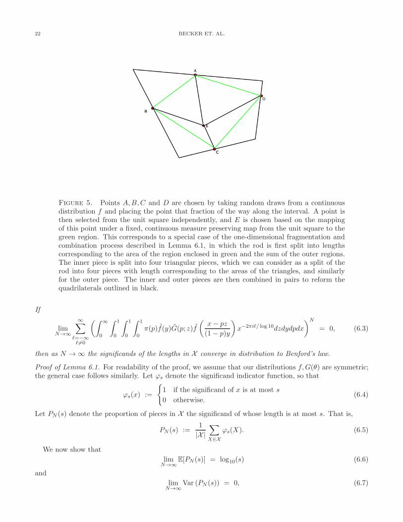
6.2. Decomposition of Quadrilaterals. We now consider our model for decomposing convex quadrilat-erals. We will describe the construction process in detail below, illustrating it in Figure 5.

We first set some notation, and then state and prove a lemma which allows us to reduce the 2-dimensionalfragmentation to 1-dimensional problems that our techniques can handle.

Let

Sk := {x ∈ (0, 1)k : x1 + · · ·+ xk = 1}, (6.1)

and for any probability distribution f on Sk let f be its first marginal, i.e.,

f(x) =

∫ 1

y2=0· · ·∫ 1

yk=0f(x, y2, . . . , yk)dy2 · · · dyk. (6.2)

A key lemma is a variant of the unrestricted fragmentation process in which pieces are allowed to rejoinafter breaks. We state and prove it in greater generality than is needed for our construction, as theadditional freedom may be of independent interest and is no harder to state and prove.

Lemma 6.1. Fix a probability density π on (0, 1), a probability density f on Sk, and a one-parameterprobability density G(θ) on Sk depending on a single random variable θ such that (6.3) below holds. Givena stick of length L, we perform the following iterated process.

1. Break the stick at a proportion p chosen according to π.2. Break one of the pieces into k sub-pieces X1, . . . ,Xk with proportions chosen according to f .3. Independently break the other piece into k sub-pieces Y1, . . . , Yk with proportions according to G(p).4. Combine each piece Xi with the piece Yi, so that we have k pieces of lengths X1 + Y1, . . . ,Xk + Yk.5. Repeat this process independently on each of the k resulting sub-pieces until there are kN pieces X .

22 BECKER ET. AL.

Figure 5. Points A,B,C and D are chosen by taking random draws from a continuousdistribution f and placing the point that fraction of the way along the interval. A point isthen selected from the unit square independently, and E is chosen based on the mappingof this point under a fixed, continuous measure preserving map from the unit square to thegreen region. This corresponds to a special case of the one-dimensional fragmentation andcombination process described in Lemma 6.1, in which the rod is first split into lengthscorresponding to the area of the region enclosed in green and the sum of the outer regions.The inner piece is split into four triangular pieces, which we can consider as a split of therod into four pieces with length corresponding to the areas of the triangles, and similarlyfor the outer piece. The inner and outer pieces are then combined in pairs to reform thequadrilaterals outlined in black.

If

limN→∞

∞∑

ℓ=−∞ℓ 6=0

(∫ ∞

0

∫ 1

0

∫ 1

0

∫ 1

0π(p)f(y)G(p; z)f

(x− pz

(1− p)y

)x−2πiℓ/ log 10dzdydpdx

)N

= 0, (6.3)

then as N → ∞ the significands of the lengths in X converge in distribution to Benford’s law.

Proof of Lemma 6.1. For readability of the proof, we assume that our distributions f,G(θ) are symmetric;the general case follows similarly. Let ϕs denote the significand indicator function, so that

ϕs(x) :=

{1 if the significand of x is at most s

0 otherwise.(6.4)

Let PN (s) denote the proportion of pieces in X the significand of whose length is at most s. That is,

PN (s) :=1

|X |∑

X∈X

ϕs(X). (6.5)

We now show that

limN→∞

E[PN (s)] = log10(s) (6.6)

and

limN→∞

Var (PN (s)) = 0, (6.7)


which together suffice to prove our theorem. The proof of (6.6) proceeds as in the proof of Theorem 1.5except that we apply Theorem 1.1 of [JKKKM] with fD(θ) = 1/(θ + p/4) as opposed to fD(θ) = 1/θ. Wetherefore concentrate our attention on showing (2.9).

We have

Var (PN (s)) = E[P 2N (s)]− E[PN (s)]2

=1

42N

∑

X,Y ∈X

E[ϕs(X)ϕs(Y )]− E[PN (s)]2

=1

4NE[PN (s)] +

1

42N

∑

X 6=Y ∈X

E[ϕs(X)ϕs(Y )]− E[PN (s)]2

=1

42N

∑

X 6=Y ∈X

E[ϕs(X)ϕs(Y )]− log10(s) + o(1). (6.8)

Now, consider two arbitrary pieces X 6= Y ∈ X . Call one iteration of the process 1–5 a “cut,” each piecein X being the result of a sequence of N cuts. We can express X,Y each as a product of terms of the form

piαi + (1− pi)βi (6.9)

representing the ith cut, where pi is the proportion chosen in step 1 of our iterated process, αi is the lengthof one of the pieces Xj obtained in step 2, and βi is the length of one of the pieces Yi obtained in step 3.Since the sequences of cuts that produced X and Y may be the same up to some k < N , we express X,Ymore precisely by

X = L (p1α1 + (1− p1)β1) · · · (pk−1αk−1 + (1− pk−1)βk−1) (pkαk + (1− pk)βk)

(pk+1αk+1 + (1− pk+1)βk+1) · · · (pNαN + (1− pN )βN )

=: La1 · · · ak−1 (pkαk + (1− βk)βk) ak+1 · · · aN=: L1ak+1 · · · aN

Y = L (p1α1 + (1− p1)β1) · · · (pk−1αk−1 + (1− pk−1)βk−1)(pkα

′k + (1− pk)β

′k

)(pk+1αk+1 + (1− pk+1)βk+1

)· · ·(pN αN + (1− pN )βN

)

=: La1 · · · ak−1

(pkα

′k + (1− pk)β

′k +

p

4

)ak+1 · · · aN

=: L2ak+1 · · · aN (6.10)

where ai, ai are independent random variables. We seek to describe their distribution.Each αi, αi is some component of an independent random variable chosen according to f ; by symmetry,

we may suppose it to be the first coordinate. Thus αi, αi are independent random variables with distributionf . Likewise, the βi, βi are independent variables chosen according to G(pi). However, α′

i and β′i are not

independent. The distribution of the ai, ai has density

h(x) =

∫ 1

0φ(p)

∫ 1

0f(y)

∫ 1

0G(p; z)f

(x− pz

(1− p)y

)dzdydp. (6.11)

As in §2, we write

I(L1) =

∫ 1

ak+1=0· · ·∫ 1

aN=0ϕs

(L1

N∏

i=k+1

ai

)N∏

i=k+1

h(ai)dak+1 · · · daN

I(J2) =

∫ 1

ak+1=0· · ·∫ 1

aN=0ϕs

(L2

N∏

i=k+1

ai

)N∏

i=k+1

h(ai)dak+1 · · · daN (6.12)

so that

E[ϕs(X)ϕ(Y )] =

∫ 1

a1=0· · ·∫ 1

ak−1=0

∫ 1

αk=0

∫ 1

βk=0I(L1)J(L2)da1 · · · dak−1dαkdβk. (6.13)

24 BECKER ET. AL.

It suffices to show that, for any L1, L2, we have |I(L1)J(L2)− (log10 s)2| = o(1) in N . This is proven in §2

if h satisfies the Mellin condition (6.3). In other words if

limN→∞

∞∑

ℓ=−∞ℓ 6=0

(∫ ∞

0

∫ 1

0

∫ 1

0

∫ 1

0π(p)f(y)G(p; z)f

(x− pz

(1− p)y

)x−2πiℓ/ log 10dzdydpdx

)N

= 0, (6.14)

which is precisely (6.3) on π,f ,G. �

We can now proceed to the proof of Benford behavior in the quadrilateral decomposition model.

Proof of Theorem 1.15. Unlike in the triangular case, affine transformations do not map between arbitraryquadrilaterals, since affine transformations must preserve parallelism. However, there are numerous con-tinuous mappings from arbitrary convex quadrilaterals to squares that preserve the ratio of areas; theconstruction of Gromov after Knothe provides such a mapping with other nice properties [Gr]. The ideaof the mapping is to send slices of the first quadrilateral to slices of the second in a continuous way; see[BrMo] for details on the specific construction. Therefore, given a probability density f on the square, weobtain a unique probability density f ′ on any convex quadrilateral, and if f is uniform then so is f ′.

We now formulate our decomposition process in precise terms. We begin with the unit square, a proba-bility density f on (0, 1), and a probability density g on (0, 1)2. We independently select a point on eachside according to f . Call these A,B,C,D. We then choose a point E in the interior of the quadrilateralABCD according to the composition of g with a mapping that preserves ratios of areas. We now connect Eto each of A,B,C,D in order to decompose the square into four convex quadrilaterals. We then perform thesame decomposition independently on each of these quadrilaterals, repeating this process until we obtain4N quadrilaterals.

Again, we consider the ratios of the areas of the sub-quadrilaterals to their parent, and use the resultingdistribution to reframe this two-dimensional process as a decomposition of the rod. Because of the existenceof continuous mappings that preserve ratios of areas, it is enough to consider the decomposition of theunit square. Each sub-quadrilateral can be thought of as having two triangular components: one outsideABCD and one inside it. We will determine the distribution of the proportions of the sub-quadrilateralsby conditioning on the area of the inner quadrilateral ABCD. In terms of the decomposition of the rod,this corresponds to the following case of Lemma 6.1. We split the rod into two pieces, one correspondingto the inner quadrilateral ABCD and one corresponding to the outer area. We then split the formerpiece according to the areas of the inner triangles, and the outer piece according to the areas of the outertriangles, and then recombine the corresponding sub-pieces.

If (a, b, c, d) are the proportions of the points on each side, then the outer triangles have areas 12a(1− b),

12b(1− c), 1

2c(1− d), 12d(1− a) and the quadrilateral ABCD has area A = 1− 1

2(a(1− b) + b(1− c) + c(1−d) + d(1− a)). Let π denote the density of the probability distribution of A. Let h1(A) denote the densityof the distribution of the areas of the outer triangles conditional on A. Note that if f is continuous, then soare π and h1. Let h2 denote the density of the distribution of the ratios of the areas of the inner trianglesto A. Pulling back using any continuous area preserving mapping, we may determine the distribution ofh2 by considering the case when ABCD is the unit square. In this case, by selecting the point (x, y) weproduce triangles of area 1

2xy,12x(1 − y), 12(1 − x)y, 12(1 − x)(1 − y). The areas of the inner triangles in

ABCD are obtained by multiplying through by A. Therefore, if f and g are both continuous, we see thath2 is continuous.

Theorem 1.15 follows from applying Lemma 6.1 with this π above corresponding to the π of the lemmaand h1 and h2 corresponding to G and f , respectively. �

7. Proof of Theorem 1.17: Determinant Expansion

The techniques introduced to prove that the continuous stick decomposition processes result in Benfordbehavior can be applied to a variety of dependent systems. To show this, we prove that the n! termsof a matrix determinant expansion follow Benford’s Law in the limit as long as the matrix entries areindependent, identically distributed nice random variables. As the proof is similar to our previous results,


we content ourselves with sketching the arguments, highlighting where the differences occur. See [MaMil]for additional examples of Benford behavior in matrix ensembles.

Consider an n×n matrix A with independent identically distributed entries apq drawn from a continuousreal valued density f(x). Without loss of generality, we may assume that all entries of A are non-negative.For 1 ≤ i ≤ n!, let Xi,n be the ith term in the determinant expansion of A. Thus Xi,n =

∏np=1 apσi(p) where

the σi’s are the n! permutation functions on {1, . . . , n}.We prove that the distribution of the significands of the sequence {Xi,n}n!p=1 converges in distribution

to Benford’s Law when the entries of A are drawn from a distribution f that satisfies (1.6) (with h = f).Recall that it suffices to show

(1) limN→∞

E[Pn(s)] = log10(s), and

(2) limN→∞

Var (Pn(s)) = 0.

We first quantify the degree of dependencies, and then sketch the proofs of the mean and variance.Fix i ∈ {1, . . . , n!} and consider the number of terms Xj,n that share exactly k entries of A with Xi,n.Equivalently: If we permute the numbers 1, 2, . . . , n, how likely is it that exactly k are returned to theiroriginal starting position? This is the well known probleme des rencontres (the special case of k = 0 iscounting derangements), and in the limit the probability distribution converges to that of a Poisson randomvariable with parameter 1 (and thus the mean and variance tend to 1; see [HSW]). Therefore, if Ki,j denotesthe number of terms Xi,n and Xj,n share, the probability that Ki,j > logN is o(1).

The determination of the mean follows as before. By linearity of expectation we have

E[Pn(s)] =1

n!

n!∑

i=1

E[ϕs(Xi,n)]. (7.1)

It suffices to show that limn→∞

E[ϕs(Xi,n)] = log10 s. We have

E[ϕs(Xi,n)] =

∫

a1σi(1)

∫

a2σi(2)

· · ·∫

anσi(n)

ϕs

n∏

p=1

apσi(p)

·n∏

p=1

f(apσi(p)) da1σi(1)da2σi(2) · · · danσi(n), (7.2)

where apσi(p) are the entries of A. As these random variables are independent and f(x) satisfies (1.6), theconvergence to Benford follows from [JKKKM] (or see Appendix A of [B–]).

To complete the proof of convergence to Benford, we need to control the variance of Pn(s). Arguing asbefore gives

Var (Pn(s)) =log10(s)

n!+

1

(n!)2

n!∑

i,j=1i 6=j

E[ϕs(Xi,n)ϕs(Xj,n)]

− log210 s+ o(1). (7.3)

We then mimic the proof from §2.2. There we used that, for a fixed i, the number of the 2N pairs (i, j)with n factors not in common was 2n−1; in our case we use Ki,j is approximately Poisson distributed toshow that, with probability 1+o(1) there are at least logN different factors. The rest of the proof proceedssimilarly.

8. Future Work

Many of our results concern continuous decomposition models in which a stick is broken at a proportionp. We propose several variations of a discrete decomposition model in which a stick breaks into pieces ofinteger length, which we hope to return to in a future paper.

Consider the following additive decomposition process. Begin with a stick of length L and uniformly atrandom choose an integer length c ∈ [1, L− 1] at which to cut the stick. This results in two pieces, one of

26 BECKER ET. AL.

length c and one of length L− c. Continue this cutting process on both sticks, and only stop decomposinga stick if its length corresponds to a term in a given sequence {an}. As one cannot decompose a stick oflength one into two integer pieces, sticks of length one stop decomposing as well.

Conjecture 8.1. The stick lengths that result from this decomposition process follow Benford’s Law formany choices of {an}. In particular, if either (i) {an} = {2n} or (ii) {an} is the set of all prime numbersthen the resulting stick lengths are Benford.

More generally one can investigate processes where the stick lengths continue decomposing if they are incertain residue classes to a fixed modulus, or instead of stopping at the primes one could stop at a sequencewith a similar density, such as ⌊n log n⌋. It is an interesting question to see, for a regularly spaced sequence,the relationship between the density of the sequence and the fit to Benford’s law. While one must of coursebe very careful with any numerical exploration, as many processes are almost Benford (see for example theresults on exponent random variables in [LSE, MN2]), Theorem 1.9 is essentially a continuous analogue ofthis problem when an = 2n, and thus provides compelling support.

Figure 6(a) shows a histogram of chi-square values from numerical simulations with a χ28 distribution

overlaid (as we have 9 first digits, there are 8 degrees of freedom). A stick of length approximately 104 wasdecomposed according to the above cutting process, where {an} = 2n. A chi-square value9 was calculatedby comparing the frequencies of each digit obtained from the simulation to the frequencies predicted byBenford’s Law. If the simulated data is a good fit to Benford’s Law, the χ2 values should follow a χ2

distribution. Examining the plot below shows that our numerical simulations support Conjecture 8.1(i).Similarly, Figure 6(b), which shows the chi-square values obtained when {an} is the set of all primes,supports Conjecture 8.1(ii).

Figure 6. (a) {an = 2n}: 2500 chi-square values of stick lengths to Benford behavior afterdecomposition of sticks of length approximately 107. (b) {an = pn} (the set of primes): 1000chi-square values of stick lengths to Benford behavior after decomposition of sticks of lengthapproximately 10500.

Conjecture 8.2. Fix a monotonically increasing sequence {an}. Consider a decomposition process wherea stick whose length is in the sequence does not decompose further. The process is not Benford if {an} isany of the following: {n2}, {2n}, {Fn} where Fn is the nth Fibonacci number.

More generally, we do not expect Benford behavior if the sequence is too sparse, which is the case forpolynomial growth in n (when the exponent exceeds 1) or, even worse, geometric growth.

Figure 7 features plots of the observed digit frequencies vs the Benford probabilities. These plots alsogive the total number of fragmented pieces, the number of pieces whose lengths belong to the stoppingsequence, and the chi-squared value. Notice that the stopping sequences in Conjecture 8.2 result in stick

9If Xi are the simulation frequencies of each digit i = 1, 2, . . . , 9 and Yi are the frequencies of each digit as predicted byBenford’s Law, where i = 1, . . . , 9, then the chi-squared value we calculated is given by

∑9i=1(XiN − YiN)2/NYi, where N is

the number of pieces.


lengths with far too high a probability of being of length 1. This fact leads us to believe that the sequencesare not “dense” enough to result in Benford behavior.

In addition to proofs of the conjectures, future work could include further exploration of the relationshipbetween stopping sequence density and Benford behavior.

Figure 7. (a) {an = n2}: Distribution of stick lengths after decomposing sticks of initiallength approximately 106. (b) {an = 2n}: Distribution of stick lengths after decomposing1000 sticks of initial length approximately 10500. (c) {an = Fn}, the Fibonacci Numbers:Distribution of stick lengths after decomposing 500 sticks of initial length approximately10500.

Appendix A. Non-Benford Behavior

We consider the following generalization of the Unrestricted Decomposition Model of Theorem 1.5,where now the proportions at level n are drawn from a random variable with density φn. If there areonly finitely many densities and if the Mellin transform condition is satisfied, then the sequence of sticklengths converges to Benford; if there are infinitely many possibilities, however, then it is possible to obtainnon-Benford behavior.

Specifically, we give an example of a sequence of distributions D with the following property: If all cutproportions are drawn from any one distribution in D then the resulting stick lengths converge to Benford’sLaw, but if all cut proportions in the nth level are chosen from the nth distribution in D, the stick lengthsdo not exhibit Benford behavior.

It is technically easier to work with the densities of the logarithms of the cut proportions. Fix δ > 0 andchoose a sequence of ǫn’s so that they monotonically decrease to zero and

ǫn < min

(√3

20π2(n+ 1)2,1

2

δ

2n,log 1

2

2,1− log 1

2

2

); (A.1)

these values and the meaning of these constants will be made clear during the construction. Consider thesequence of distributions with the following densities

φn(x) =

{1

2ǫnif∣∣x− log 1

2

∣∣ < ǫn

0 otherwise;(A.2)

these will be the densities of the logarithms of the cut proportions.If the logarithm of the cut proportion is drawn solely from the distribution φk for a fixed k, then as the

number of iterations of this cut process tends to infinity the resulting stick lengths converge to Benford’sLaw. This follows immediately from Theorem 1.5 as the associated densities of the cut proportions satisfythe Mellin condition (1.6).

We show that if the logarithms of the cut proportions for the nth iteration of the decomposition processis drawn from φn then the resulting stick lengths do not converge to Benford behavior for certain δ. Whatwe do is first show that the distribution of one stick piece (say the resulting piece from always choosing theleft cut at each stage) is non-Benford, and then we prove that the ratio of the lengths of any two final piecesis approximately 1. The latter claim is reasonable as our cut proportions are becoming tightly concentratedaround 1/2; if they were all exactly 1/2 then all final pieces would be the same length.

28 BECKER ET. AL.

Instead of studying the Mellin transforms of the cut proportions we can study the Fourier coefficientsof the logarithms of the proportions (again, this is not surprising as the two transforms are related by alogarithmic change of variables). For a function φ on [0, 1], its nth Fourier coefficient is

φ(n) :=

∫ 1

0φ(x)e−2πinxdx. (A.3)

Miller and Nigrini [MN1] proved that if R1, . . . , RM are continuous independent random variables with gmthe density of log10 S10(|Rm|), then the product R1 · · ·RM converges to Benford’s law if and only if for eachnon-zero n we have limM→0 g1(n) · · · gM (0) = 0.

We show that if we take our densities to be the φn’s that the limit of the product of the Fourier coefficientsat 1 does not tend to 0. We have

φn(1) =1

2ǫn

∫ 12+ǫn

12−ǫn

e−2πixdx = −1 +2π2ǫ2n3

+O(ǫ4n). (A.4)

As we are assuming ǫn <√

320π2(n+1)2 , we find for n large that

∣∣∣φn(1)∣∣∣ ≥ n2 + 2n

(n+ 1)2. (A.5)

As

limN→∞

N∏

n=1

n2 + 2n

(n + 1)2=

1

2, (A.6)

we see that

limN→∞

N∏

n=1

∣∣∣φ1(1) · · · φN (1)∣∣∣ > 0. (A.7)

This argument shows that the product of N random variables, where the logarithm of the nth variableis drawn from the distribution φn, is not Benford. This product is analogous to the length of one of the 2N

sticks that are created after N iterations of our cut process. To show the entire collection of stick lengthsdoes not follow a Benford distribution, we argue that all of the lengths are virtually identical because thecutting proportion tends to 1/2 (specifically, that the ratio of any two lengths is approximately 1).

Let us denote the lengths of the sticks left after the N th iteration of our cutting procedure by XN,i, where

i = 1, . . . , 2N . Each length is a product of N random variables; the nth term in the product is either pn (or1− pn), where the logarithm of pn is drawn from the distribution φn. Proving the ratio of any two lengthsis approximately 1 is the same as showing that log(XNi/XN,j) is approximately 0. If we can show thelargest ratio has a logarithm close to 0 then we are done. The largest (and similarly smallest) ratio comeswhen XN,i and XN,j have no terms in common, as then we can choose one to have the largest possible cutat each stage and the other the smallest possible cut. Thus XN,i always has the largest possible cut; as the

largest logarithm at the nth stage is ǫn + log 12 , its proportion at the nth level is eǫn+log 1

2 . Similarly XN,j

always has the smallest cut, which at the nth level is e−ǫn+log 12 . Therefore

logXN,i

XN,j= log

N∏

n=1

eǫn+log 12

e−ǫn+log 12

=

N∑

n=1

2ǫn; (A.8)

as we chose ǫn < 12

δ2n , the maximum ratio between two pieces is at most δ. By choosing δ sufficiently small

we can ensure that all the pieces have approximately the same significands (for example, if δ < 10−2014

then we cannot get all possible first digits).


Appendix B. Notes on Lemons’ Work

In his 1986 paper, On the Number of Things and the Distribution of First Digits, Lemons [Lem] modelsa particle decomposition process and offers it as evidence for the prevalence of Benford behavior, arguingthat many sets that exhibit Benford behavior are merely the breaking down of some conserved quantity.However, Lemons is not completely mathematically rigorous in his analysis of the model (which he statesin the paper), and glosses over several important technical points. We briefly mention some issues, such asconcerns about the constituent pieces in the model as well as how the initial piece decomposes. We discussour resolutions of these issues as well as their impacts on the behavior of the system.

The first issue in Lemons’ model concerns the constituent pieces. He assumes the set of possible piecesizes is bounded above and below and is drawn from a finite set, eventually specializing to the case wherethe sizes are in a simple arithmetic progression (corresponding to a uniform spacing), and then taking alimit to assume the pieces are drawn from a continuous range. In this paper, we allow our piece lengths tobe drawn continuously from intervals at the outset, and not just in the limit. This removes some, but byno means all, of the technical complications. One must always be careful in replacing discrete systems withcontinuous ones, especially as there can be number-theoretic restrictions on which discrete systems have asolution. Modeling any conserved quantity is already quite hard with the restriction that the sum of allparts must total to the original starting amount; if the pieces are forced to be integers then certain numbertheoretic issues arise. For example, imagine our pieces are of length 2, 4 or 6, so we are trying to solve2x1 + 4x2 + 6x3 = n. There are no solutions if n = 2017, but there are 85,345 if n is 2018. By consideringa continuous system from the start, we avoid these Diophantine complications; see [IMS] for an analysis ofthe discrete setting.

A second issue missing from Lemons argument is how the conserved quantity, the number of pieces,and the piece sizes should be related. The continuous limit thus requires consideration of three quantities.Without further specification of their relative scaling, the power law distribution (which leads to Benfordbehavior) is but one possible outcome. Statistical models of the fragmentation of a conserved quantitybased on integer partitioning have been constructed [ChaMek, LeeMek, Mek]. These models can lead to apower law distribution but only for special weightings for the different partitions. Whether this distributioncan be obtained from equally weighted partitions (as used in Lemons argument) is an important question,to which we hope to return.

A related issue is that it is unclear how the initial piece breaks up. The process is not described explicitly,and it is unclear how likely some pieces are relative to others. Finally, while he advances heuristics todetermine the means of various quantities, there is no analysis of variances or correlations. This meansthat, though it may seem unlikely, the averaged behavior could be close to Benford while most partitionswould be far from Benford.10

These are important issues, and their resolution and model choice impacts the behavior of the system.We mention a result from Miller-Nigrini [MN2], where they prove that while order statistics are close toBenford’s Law (base 10), they do not converge in general to Benford behavior. In particular, this meansthat if we choose N points randomly on a stick of length L and use those points to partition our rod, thedistribution of the resulting piece sizes will not be Benford. Motivated by this result and Lemons’ paper,we instead considered a model where at stage N we have 2N sticks of varying lengths, and each stick isbroken into two smaller sticks by making a cut on it at some proportion. Each cut proportion is chosenfrom the unit interval according to a density f . Dependencies clearly exist within this system as the lengthsof final sticks must sum to the length of the starting stick.

References

[Adh] A. K. Adhikari, Some results on the distribution of the most significant digit, Sankhya: The Indian Journal ofStatistics, Series B 31 (1969), 413–420.

10Imagine we toss a coin one million times, always getting either all heads or all tails. Let’s say these two outcomes areequally likely. If we were to perform this process trillions of times, the total number of heads and tails would be close to eachother; however, no individual experiment would be close to 50%.

30 BECKER ET. AL.

[AS] A. K. Adhikari and B. P. Sarkar, Distribution of most significant digit in certain functions whose arguments arerandom variables, Sankhya: The Indian Journal of Statistics, Series B 30 (1968), 47–58.

[AF] R. L. Adler and L. Flatto, Uniform distribution of Kakutanis interval splitting procedure, Z. Wahrscheinlichkeits-theorie und Verw. Gebiete 38 (1977), no. 4, 253–259.

[ARS] T. Anderson, L. Rolen and R. Stoehr, Benford’s Law for Coefficients of Modular Forms and Partition Functions,Proc. Am. Math. Soc. 139 (2011), no. 5, 1533–1541.

[B–] T. Becker, D. Burt, T. C. Corcoran, A. Greaves-Tunnell, J. R. Iafrate, J. Jing, S. J. Miller, J. D. Porfilio, R. Ronan,J. Samranvedhya, F. Strauch, and B. Talbut, Benford’s Law and Continuous Dependent Random Variables, arXivversion. http://arxiv.org/pdf/1309.5603.

[Ben] F. Benford, The law of anomalous numbers, Proceedings of the American Philosophical Society 78 (1938), 551-572.[Ber1] A. Berger, Multi-dimensional dynamical systems and Benford’s Law, Discrete Contin. Dyn. Syst. 13 (2005), 219–

237.[Ber2] A. Berger, Benford’s Law in power-like dynamical systems 5 (2005), Stoch. Dyn., 587–607.[BBH] A. Berger, Leonid A. Bunimovich and T. Hill, One-dimensional dynamical systems and Benford’s Law, Trans.

Amer. Math. Soc. 357 (2005), no. 1, 197-219.[BH1] A. Berger and T. P. Hill, Newton’s method obeys Benford’s Law, American Mathematical Monthly 114 (2007),

588–601.[BH2] A. Berger, and T. P. Hill, Benford Online Bibliography, http://www.benfordonline.net.[BH3] A. Berger and T. P. Hill, Fundamental flaws in Feller’s classical derivation of Benford’s Law, Preprint, University

of Alberta, 2010.[BH4] A. Berger and T. P. Hill, Benford’s Law strikes back: No simple explanation in sight for mathematical gem, The

Mathematical Intelligencer 33 (2011), 85–91.[BH5] A. Berger and T. P. Hill, A Basic Theory of Benford’s Law, Probab. Surv. 8 (2011), 1–126.[BH6] A. Berger and T. P. Hill, An Introduction to Benford’s Law, Princeton University Press, Princeton, 2015.[BHKR] A. Berger, T. P. Hill, B. Kaynar and A. Ridder, Finite-state Markov Chains Obey Benford’s Law, to appear in

SIAM J. Matrix Analysis.[Bert] J. Bertoin, Random fragmentation and coagulation processes, Cambridge Studies in Advanced Mathematics 102,

Cambridge University Press, Cambridge, 2006.[Bh] R. N. Bhattacharya, Speed of convergence of the n-fold convolution of a probability measure on a compact group, Z.

Wahrscheinlichkeitstheorie verw. Geb. 25 (1972), 1–10.[BrDu] M. D. Brennan and R. Durrett, Splitting intervals, Ann. Probab. 14 (1986), no. 3, 1024–1036.[BrMo] J. Brothers and F. Morgan, The isoperimetric theorem for general integrands, Michigan Math. J. 41 (1994), no. 3,

419–431.[Buc] B. Buck, A. Merchant and S. Perez, An Illustration of Benford’s First Digit Law Using Alpha Decay Half-Lives,

European Journal of Physics 14 (1993), 59–63.[Ca] I. Carbone, Discrepancy of LS-sequences of partitions and points, Ann. Mat. Pura Appl. 191 (2012), 819–844.[CaVo] I. Carbone and A. Volcic, Kakutani’s splitting procedure in higher dimension, Rend. Istit. Mat. Univ. Trieste 39

(2007), 119–126.[ChaMek] K. C. Chase and A. Z. Mekjian, Nuclear fragmentation and its parallels, Physical Review C 49 (1994), 2164.[Che] H. Chen, On the Summation of First Subseries in Closed Form, International Journal of Mathematical Education

in Science and Technology 41 (2010), no. 4, 538–547.[CLTF] E. Costasa, V. Lopez-Rodasa, F. J. Torob, A. Flores-Moya, The number of cells in colonies of the cyanobacterium

Microcystis aeruginosa satisfies Benford’s Law, Aquatic Botany 89 (2008), no. 3, 341–343.[CLM] V. Cuff, A. Lewis and S. J. Miller, The Weibull distribution and Benford’s Law, preprint.[Dia] P. Diaconis, The distribution of leading digits and uniform distribution mod 1, Ann. Probab. 5 (1979), 72-81.[DrNi] P. D. Drake and M. J. Nigrini, Computer assisted analytical procedures using Benford’s Law, Journal of Accounting

Education 18 (2000), 127–146.[El] I. Eliazar, Harmonic statistics, Annals of Physics 380 (2017), 168–187.[GS] G. R. Grimmett and D. R. Stirzaker, Probability and random processes (2009), 2nd edition, Clarendon Press,

Oxford.[Gr] M. Gromov, Isoperimetric inequalities in Riemannian manifolds, Appendix I to Asymptotic Theory of Finite

Dimensional Normed Spaces by Vitali D. Milman and Gideon Schechtman, Lecture Notes in Mathematics, No.1200. Springer-Verlag, New York, 1986.

[HSW] D. Hanson, K. Seyffarth and J. H. Weston, Matchings, Derangements, Rencontres, Mathematics Magazine 56

(1983), no. 4, 224–229.[Hi1] T. Hill, The first-digit phenomenon, American Scientists 86 (1996), 358-363.[Hi2] T. Hill, A statistical derivation of the significant-digit law, Statistical Science 10 (1996), 354-363.[HS] M. Hindry and J. Silverman, Diophantine geometry: An introduction, Graduate Texts in Mathematics 201,

Springer, New York, 2000.[Hu] W. Hurlimann, Benford’s Law from 1881 to 2006, http://arxiv.org/pdf/math/0607168.

http://arxiv.org/pdf/1309.5603

http://www.benfordonline.net

http://arxiv.org/pdf/math/0607168


[IMS] J. Iagrate, S. J. Miller and F. Strauch, Equipartitions and a distribution for numbers: A statistical model forBenford’s law, Physical Review E 91 (2015), no. 6, 062138 (6 pages).

[IV] M. Infusino and A. Volcic, Uniform distribution on fractals, Unif. Distrib. Theory 4 (2009), no. 2, 47–58.[JKKKM] D. Jang, J. U. Kang, A. Kruckman, J. Kudo and S. J. Miller, Chains of distributions, hierarchical Bayesian models

and Benford’s Law, Journal of Algebra, Number Theory: Advances and Applications, volume 1, number 1 (March2009), 37–60.

[JN] S. Janson and R. Neininger, The size of random fragmentation trees, Probab. Theory Related Fields 142 (2008),no. 3-4, 399–442.

[JR] E. Janvresse and T. de la Rue, From uniform distribution to Benford’s Law, Journal of Applied Probability 41

(2004) no. 4, 1203–1210.[Ka] S. Kakutani, A problem of equidistribution on the unit interval [0, 1], Measure theory (Proc. Conf., Oberwolfach,

1975), Lecture Notes in Math., Vol. 541, Springer, Berlin, 1976, pp. 369–375.[Knu] D. Knuth, The Art of Computer Programming, Volume 2: Seminumerical Algorithms, 3rd edition, Addison-Wesley,

MA, 1997.[Kol] A. N. Kolmogoroff, Uber das logarithmisch normale Verteilungsgesetz der Dimensionen der Teilchen bei

Zerstuckelung, C. R. (Doklady) Acad. Sci. URSS (N. S.) 31 (1941), 99–101.[KonMi] A. Kontorovich and S. J. Miller, Benford’s Law, values of L-functions and the 3x + 1 problem, Acta Arith. 120

(2005), 269–297.[KN] L. Kuipers and H. Niederreiter, Uniform Distribution of Sequences, John Wiley & Sons, 1974.[LS] J. Lagarias and K. Soundararajan, Benford’s Law for the 3x+ 1 Function, J. London Math. Soc. 74 (2006), series

2, no. 2, 289–303.[LeeMek] S. J. Lee and A. Z. Mekjian, Canonical studies of the cluster distribution, dynamical evolution, and critical tem-

preature in nuclear multifragmentation processes, Physical Review C 45 (1992), 1284.[LSE] L. M. Leemis, B. W. Schmeiser and D. L. Evans, Survival Distributions Satisfying Benford’s Law, The American

Statistician 54 (2000), no. 4, 236–241.[Lem] D. S. Lemons, On the number of things and the distribution of first digits, Am. J. Phys. 54 (1986), no. 9, 816–817.[Lev1] P. Levy, Theorie de l’Addition des Variables Aleatoires, Gauthier-Villars, Paris, 1937.[Lev2] P. Levy, L’addition des variables aleatoires definies sur une circonference, Bull. de la S. M. F. 67 (1939), 1–41.[Lo] J. C. Lootgieter, Sur la repartition des suites de Kakutani. I, Ann. Inst. H. Poincare Sect. B (N.S.) 13 (1977), no.

4, 385–410.[MaMil] C. Manack and S. J. Miller, Leading Digit Laws on Linear Lie Groups, Research in Number Theory (2015) 1:22,

DOI 10.1007/s40993-015-0024-4.[Meb] W. Mebane, Detecting Attempted Election Theft: Vote Counts, Voting Machines and Benford’s Law, Prepared for

delivery at the 2006 Annual Meeting of the Midwest Political Science Association, April 20-23, Palmer House,Chicago. http://www.umich.edu/~wmebane/mw06.pdf.

[Mek] A. Z. Mekjian, Model of a fragmentation process and its power-law behavior, Physical Review Letters 64 (1990),2125.

[Mil] S. J. Miller (editor), Theory and Applications of Benford’s Law, Princeton University Press, 2015, 438 pages.[MN1] S. J. Miller and M. Nigrini, The Modulo 1 Central Limit Theorem and Benford’s Law for Products, International

Journal of Algebra 2 (2008), no. 3, 119–130.[MN2] S. J. Miller and M. Nigrini, Order statistics and Benford’s Law, International Journal of Mathematics and Mathe-

matical Sciences, Volume 2008 (2008), Article ID 382948, 19 pages. doi:10.1155/2008/382948[MN3] S. J. Miller and M. Nigrini, Data diagnostics using second order tests of Benford’s Law, Auditing: A Journal of

Practice and Theory 28 (2009), no. 2, 305–324. doi: 10.2308/aud.2009.28.2.305[MT-B] S. J. Miller and R. Takloo-Bighash, An Invitation to Modern Number Theory, Princeton University Press, Princeton,

NJ, 2006.[MorSPZ] M. Moret, V. de Senna, M. Pereira and G. Zebende, Newcomb-Benford Law in Astrophysical Sources, International

Journal of Modern Physics C 17 (2006), no. 11, 1597–1604.[MorSSZ] M. Moret, V. de Senna, M. Santana and G. Zebende, Geometric Structural Aspects of Proteins and Newcomb-

Benford Law, International Journal of Modern Physics C 20 (2009), no. 12, 1981–1988.[New] S. Newcomb, Note on the frequency of use of the different digits in natural numbers, Amer. J. Math. 4 (1881),

39-40.[NiRen] D. Ni and Z. Ren, Benford’s Law and Half-Lives of Unstable Nuclei, European Physical Journal A 38 (2008),

251–255.[NiWeRe] D. Ni, L. Wei and Z. Ren, Benford’s Law and β-Decay Half-Lives, Communications in Theoretical Physics 51

(2009), 713–716.[Nig1] M. Nigrini, The Detection of Income Tax Evasion Through an Analysis of Digital Frequencies, PhD thesis, Univer-

sity of Cincinnati, OH, USA, 1992.[Nig2] M. Nigrini, Using Digital Frequencies to Detect Fraud, The White Paper 8 (1994), no. 2, 3–6.

http://www.umich.edu/~wmebane/mw06.pdf

32 BECKER ET. AL.

[Nig3] M. Nigrini, Digital Analysis and the Reduction of Auditor Litigation Risk. Pages 69–81 in Proceedings of the 1996Deloitte & Touche / University of Kansas Symposium on Auditing Problems, ed. M. Ettredge, University of Kansas,Lawrence, KS, 1996.

[NM] M. Nigrini and S. J. Miller, Benford’s Law applied to hydrology data – results and relevance to other geophysicaldata, Mathematical Geology 39 (2007), no. 5, 469–490.

[NigMi] M. Nigrini and L. Mittermaier, The Use of Benford’s Law as an Aid in Analytical Procedures, Auditing: A Journalof Practice & Theory 16 (1997), no. 2, 52–67.

[Ol] J. Olli, Division point measures resulting from triangle subdivisions, Geom. Dedicata 158 (2012), 69–86.[PHA] F. Perez-Gonzalez, G. L. Heileman, and C.T. Abdallah, Benford’s Law in Image Processing, Proceedings of the

IEEE International Conference on Image Processing (ICIP), San Antonio, TX, Volume 1, 2007, pp. 405–408.[PTTV] L. Pietronero, E. Tosatti, V. Tosatti and A. Vespignani, Explaining the Uneven Distribution of Numbers in Nature:

the Laws of Benford and Zipf, Physica A: Statistical Mechanics and its Applications, 2001.[Pin] R. Pinkham, On the Distribution of First Significant Digits, The Annals of Mathematical Statistics 32, no. 4 (1961),

1223-1230.[PvZ] R. Pyke and W. R. van Zwet, Weak convergence results for the Kakutani interval splitting procedure, Ann. Probab.

32 (2004), no. 1A, 380–423.[Rai] R. A. Raimi, The first digit problem, Amer. Math. Monthly 83 (1976), no. 7, 521–538.[Rob] H. Robbins, On the equidistribution of sums of independent random variables, Proc. Amer. Math. Soc. 4 (1953),

786–799.[Rod] R. Rodriguez, First significant digit patterns from mixtures of uniform digits, The American Statistician, 2004.[Ro] K. Roth, Rational approximations to algebraic numbers, Mathematika 2 (1955), 1-20.[Sa] H. Sakamoto, On the distributions of the product and the quotient of the independent and uniformly distributed

random variables, Tohoku Math. J. 49 (1943), 243–260.[Sc1] P. Schatte, On sums modulo 2π of independent random variables, Math. Nachr. 110 (1983), 243–261.[Sc2] P. Schatte, On the asymptotic uniform distribution of sums reduced mod 1, Math. Nachr. 115 (1984), 275–281.[Sc3] P. Schatte, On the asymptotic logarithmic distribution of the floating-point mantissas of sums, Math. Nachr. 127

(1986),7–20.[ShaMa1] L. Shao and B. Ma, First Digit Distribution of Hadron Full Width, Modern Physics Letters A 24 (2009), no. 40,

3275–3282.[ShaMa2] L. Shao and B. Ma, Empirical Mantissa Distributions of Pulsars, Astroparticle Physics 33 (2010), 255–262.[Sl] E. Slud, Entropy and maximal spacings for random partitions, Z. Wahrscheinlichkeitstheorie und Verw. Gebiete 41

(1977/78), no. 4, 341–352.[Son] J. Sondow, Irrationality Meausres, Irrationality Bases, and a Theorem of Jarnık. http://arxiv.org/ftp/math/

papers/0406/0406300.pdf.[SS1] E. Stein and R. Shakarchi, Fourier Analysis: An Introduction, Princeton University Press, Princeton, NJ, 2003.[SS2] E. Stein and R. Shakarchi, Complex Analysis, Princeton University Press, Princeton, NJ, 2003.[ST] M. D. Springer and W. E. Thompson, The distribution of products of independent random variables, SIAM J. Appl.

Math. 14 (1966) 511–526.[To] K-H Todter, Benford’s Law as an Indicator of Fraud in Economics, German Economic Review 10 (2009), 339–351.[vZ] W. R. van Zwet, A proof of Kakutania’s conjecture on random subdivision of longest intervals, Ann. Probability 6

(1978), no. 1, 133–137.[V-BFJ] S. B. Villas-Boas, Q. Fu and G. Judge, Benford’s law and the FSD distribution of economic behavioral micro data,

Physica A: Statistical Mechanics and its Applications 2017, 711–719.

E-mail address: [email protected]

Smith College, Northampton, MA 01063


Williams College, Williamstown, MA 01267


UCLA, Los Angeles, CA 90095


Department of Statistics, University of Washington, Seattle, WA 98195


http://arxiv.org/ftp/math/papers/0406/0406300.pdf

http://arxiv.org/ftp/math/papers/0406/0406300.pdf

mailto:[email protected]






University of Michigan, Ann Arbor, MI 48109



E-mail address: [email protected], [email protected]

Department of Mathematics and Statistics, Williams College, Williamstown, MA 01267




CUNY Ph.D. Program in Mathematics, The Graduate Center, New York, NY 10016


NC State, Raleigh, NC 27695


Department of Physics, Williams College, Williamstown, MA 01267


University of California Los Angeles, Los Angeles, CA 90095



[email protected]






benford’s law and continuous dependent …€™s law and continuous dependent random variables...

Documents