benjamin geiger from few to many particles: semiclassical
TRANSCRIPT
From few to many particles:
Semiclassical approaches to
interacting quantum systems
Benjamin Geiger
55
Dis
sert
atio
nsr
eih
e Ph
ysik
- B
and
55
Ben
jam
in G
eig
er
While modern computational methods provide a powerful approach to predict the behavior of physical systems, gaining intuition of emergent phenomena requires almost invariably the use of approx-imation methods. The ideas and methods of semiclassical physics presented in this thesis provide a systematic road to address non-per-turbative regimes, where classical information find its way into the description of quantum properties of systems of few to many inter-acting particles.
The first part of the thesis provides a semiclassical description of few-particle systems using cluster expansions and novel analytic results for short-range interacting bosons in one and three dimen-sions are derived. In the second part, complementary approaches for many-particle systems are used to study the non-equilibrium scram-bling dynamics in quantum-critical bosonic systems with large parti-cle numbers, revealing an unscrambling mechanism due to criticality that is verified in extensive numerical simulations.
ISBN 978-3-86845-164-1
Umschlag_164_Geiger_Physik.indd Alle SeitenUmschlag_164_Geiger_Physik.indd Alle Seiten 20.07.20 09:5220.07.20 09:52
Benjamin Geiger
From few to many particles: Semiclassical approaches to interacting quantum systems
Titelei_164_Geiger_Physik.indd 1Titelei_164_Geiger_Physik.indd 1 19.07.20 13:0119.07.20 13:01

Herausgegeben vom Präsidium des Alumnivereins der Physikalischen Fakultät:Klaus Richter, Andreas Schäfer, Werner Wegscheider
Dissertationsreihe der Fakultät für Physik der Universität Regensburg, Band 55
From few to many particles: Semiclassical approaches to interacting quantum systems
Dissertation zur Erlangung des Doktorgrades der Naturwissenschaften (Dr. rer. nat.)der Fakultät für Physik der Universität Regensburgvorgelegt von
Benjamin Geiger
aus Radolfzell am Bodenseeim April 2020
Die Arbeit wurde von Prof. Dr. Klaus Richter angeleitet.Das Promotionsgesuch wurde am 11.03.2020 eingereicht.Das Kolloquium fand am 29.05.2020 statt.
Prüfungsausschuss: Vorsitzender: Prof. Dr. Jascha Repp 1. Gutachter: Prof. Dr. Klaus Richter 2. Gutachter: Prof. Dr. Ferdinand Evers weiterer Prüfer: Prof. Dr. Christoph Lehner
Titelei_164_Geiger_Physik.indd 2Titelei_164_Geiger_Physik.indd 2 19.07.20 13:0119.07.20 13:01

Benjamin Geiger
From few to many particles:
Semiclassical approaches to
interacting quantum systems
Titelei_164_Geiger_Physik.indd 3Titelei_164_Geiger_Physik.indd 3 19.07.20 13:0119.07.20 13:01
Bibliografische Informationen der Deutschen Bibliothek.Die Deutsche Bibliothek verzeichnet diese Publikationin der Deutschen Nationalbibliografie. Detailierte bibliografische Daten sind im Internet über http://dnb.ddb.de abrufbar.
1. Auflage 2020© 2020 Universitätsverlag, RegensburgLeibnizstraße 13, 93055 Regensburg
Konzeption: Thomas Geiger Umschlagentwurf: Franz Stadler, Designcooperative Nittenau eGLayout: Benjamin Geiger Druck: Docupoint, MagdeburgISBN: 978-3-86845-164-1
Alle Rechte vorbehalten. Ohne ausdrückliche Genehmigung des Verlags ist es nicht gestattet, dieses Buch oder Teile daraus auf fototechnischem oder elektronischem Weg zu vervielfältigen.
Weitere Informationen zum Verlagsprogramm erhalten Sie unter:www.univerlag-regensburg.de
Titelei_164_Geiger_Physik.indd 4Titelei_164_Geiger_Physik.indd 4 19.07.20 13:0119.07.20 13:01

From few to many particles: Semiclassical
approaches to interacting quantum systems
Dissertation
zur Erlangung des Doktorgrades
der Naturwissenschaften (Dr. rer. nat.)der Fakultat fur Physik
der Universitat Regensburg
vorgelegt von
Benjamin Geiger
aus
Radolfzell am Bodensee
April 2020

Promotionsgesuch eingereicht am: 11.03.2020
Die Arbeit wurde angeleitet von: Prof. Dr. Klaus Richter

List of used acronyms:
1D – one-dimensional/one dimension3D – three-dimensional/three dimensionsBCS – Bardeen-Cooper-SchriefferBEC – Bose-Einstein-condensation/condensateBGS – Bohigas-Giannoni-SchmitEBK – Einstein-Brillouin-KellerLL – Lieb-LinigerOTOC – out-of-time-ordered correlatorQCE – quantum cluster expansionRG – renormalization groupSPA – stationary phase approximationWKB – Wentzel-Kramers-Brillouin
iii


Contents
Introduction 1
From few to many . . . . . . . . . . . . . . . . . . . . . . . . . . . . . . . . . . . 1
From many to few: the advent of ultracold atom gases . . . . . . . . . . . . . . . 4
The power of semiclassical methods . . . . . . . . . . . . . . . . . . . . . . . . . 5
Outline of the thesis 9
1. Quantum cluster expansions in short-time approximation 11
1.1. Introduction . . . . . . . . . . . . . . . . . . . . . . . . . . . . . . . . . . . 11
1.2. The quantum cluster expansion . . . . . . . . . . . . . . . . . . . . . . . . 13
1.2.1. Ursell operators and symmetrization . . . . . . . . . . . . . . . . . . 14
1.2.2. The role of (irreducible) diagrams . . . . . . . . . . . . . . . . . . . 17
1.2.3. Partial traces, recurrence relations, and expectation values . . . . . 20
1.2.4. Generalization to multiple species . . . . . . . . . . . . . . . . . . . 27
1.2.5. Resummation of clusters . . . . . . . . . . . . . . . . . . . . . . . . 29
1.3. Short times—smooth spectra—high temperatures . . . . . . . . . . . . . . 34
1.3.1. Short-time propagation and high-temperature scaling . . . . . . . . 34
1.3.2. The smooth density of states/microcanonical ensemble . . . . . . . 38
1.3.3. The QCE(n)—general results . . . . . . . . . . . . . . . . . . . . . . 40
1.3.4. The thermodynamic limit and ensemble equivalence . . . . . . . . . 44
1.3.5. The shifting method from a different viewpoint . . . . . . . . . . . . 48
1.4. Application: Nonlocal correlations in the Lieb-Liniger gas . . . . . . . . . 53
1.4.1. Nonlocal correlations . . . . . . . . . . . . . . . . . . . . . . . . . . 53
1.4.2. The model . . . . . . . . . . . . . . . . . . . . . . . . . . . . . . . . 55
1.4.3. Lieb-Liniger model for three particles—full cluster expansion . . . . 56
1.4.4. Exploiting the universal scaling of the short-time approximation . . 58
1.4.5. Truncated cluster expansion for higher particle numbers . . . . . . 59
1.4.6. The thermodynamic limit . . . . . . . . . . . . . . . . . . . . . . . . 61
1.4.7. Summary and possible further applications . . . . . . . . . . . . . . 62
1.5. Application: Short-range interaction in three dimensions . . . . . . . . . . 64
1.5.1. The QCE(1) in three dimensions . . . . . . . . . . . . . . . . . . . . 64
1.5.2. Low-energy approximations and s-wave scattering . . . . . . . . . . 66
1.5.3. The short-range interacting Bose gas . . . . . . . . . . . . . . . . . 73
1.5.4. The unitary Fermi gas—a few-particle perspective . . . . . . . . . . 78
1.6. Summary and concluding remarks . . . . . . . . . . . . . . . . . . . . . . . 84
v

Contents
2. A semiclassical treatment of quantum critical phenomena 872.1. Introduction and concepts . . . . . . . . . . . . . . . . . . . . . . . . . . . 87
2.1.1. Theoretical description of phase transitions . . . . . . . . . . . . . . 872.1.2. The quantum – classical correspondence . . . . . . . . . . . . . . . 892.1.3. Phase-Space Representations . . . . . . . . . . . . . . . . . . . . . . 912.1.4. WKB wave functions and EBK torus quantization . . . . . . . . . . 932.1.5. The out-of-time-ordered correlator . . . . . . . . . . . . . . . . . . . 94
2.2. The attractive Lieb-Liniger gas in 3-mode approximation . . . . . . . . . . 992.2.1. 3-mode approximation . . . . . . . . . . . . . . . . . . . . . . . . . 1012.2.2. Semiclassical treatment . . . . . . . . . . . . . . . . . . . . . . . . . 1022.2.3. Phase space representation: Husimi functions . . . . . . . . . . . . 1152.2.4. The out-of-time-ordered correlator close to criticality . . . . . . . . 1182.2.5. Perturbation with external potential . . . . . . . . . . . . . . . . . . 129
2.3. The attractive Lieb-Liniger gas in 5-mode approximation . . . . . . . . . . 1332.3.1. Classical phase space analysis . . . . . . . . . . . . . . . . . . . . . 1342.3.2. Quantum-mechanical treatment . . . . . . . . . . . . . . . . . . . . 1382.3.3. Separation of scales and Born-Oppenheimer-type approximations . 1402.3.4. Rigidity of (excited states) quantum phase transition . . . . . . . . 147
2.4. Summary and concluding remarks . . . . . . . . . . . . . . . . . . . . . . . 151
Conclusion 153
A. Proof of equation (1.47) 159
B. Lieb-Liniger model 161
C. Propagator for shell potential 169
D. Inverse Laplace transform of special functions 173
E. Five-mode approximation 181
vi
Introduction
A great success of theoretical physics lies in the stepwise combination of small, special-ized theories to more fundamental, unified ones, that require a smaller set of assump-tions or parameters. While the discovery of each successful unification is usually drivenby the insufficiency of older theories, their greatest value lies in the prediction of newphenomena. However, although the new theories often add important new aspects tothe theoretical description of the physical effects that had been well explained withoutthem, the “old” theory can remain equally valid in such situations. Even within a singletheoretical framework, very different (equivalent) approaches, as well as approximatemethods can be formulated, that can lead to very different (approximately) equivalentinterpretations. The practical implication of this is nicely summarized in a quote byRichard Feynman, stating that “[. . . ] every theoretical physicist who is any good knowssix or seven different theoretical representations for exactly the same physics” [1]. Thiscan, of course, not be applied to new experimental discoveries, where sometimes nota single theoretical representation is known, but it describes very well how a physicalproblem should be approached from as many different viewpoints as possible to captureall of its physical aspects. However, it is not the task of a single physicist to find all theserepresentations, and in the study of new phenomena, it is usually a whole communitythat works on very similar problems, hopefully exploring them in different ways.
This thesis tries to complement some of the standard approaches that are nowadaysused in few- and many-body systems with selected semiclassical methods. The latter are,although approximate (but not perturbative) in nature, a very useful tool when it comesto acquiring a physical intuition to otherwise “black box” exact techniques, and cancomplement the understanding gained from other (approximate) methods in otherwiseinaccessible regimes. To point out some of the advantages of semiclassical methods,a brief overview of some standard methods and stepping stones in the treatment offew- and many-body systems is given in the following. It is far from being a completesummary of methods and means only to highlight some of the common characteristicsand shortcomings that set the basis for the theoretical work in the main part.
From few to many
Single-particle problems, formally also comprising the relative motion in separable two-body problems, have clearly been of paramount importance in the early developmentof quantum mechanics. The Bohr-Sommerfeld quantization of the hydrogen atom wasone of the first steps towards a full quantum theory. Once found, the latter had to betested by applying it to the simplest and best explored kinds of systems, i.e., classicallyseparable (single-particle) systems like the harmonic oscillator, the Coulomb problem,
1
Introduction
and many other systems that can be treated exactly in quantum mechanics. However,these systems are very special and already at the level of the three-body problem, oneusually obtains classically chaotic behavior [2]. In the same way, the quantum descriptionof systems with more than two interacting particles does not allow for a fully analyticdescription in most cases1 and approximate methods have to be found.
The simplest approximations, especially used in molecular and condensed matterphysics, comprise the linear combination of atomic orbitals and tight binding approxima-tions, often combined with Born-Oppenheimer approximations to adiabatically separatethe fast electronic motion from the motion of the heavy nuclei [4–6]. A first importantstepping stone in the description of atoms and molecules that included the nontrivialeffects of the interactions between the electrons was the introduction of the Hartree-Fockmethod as a many-body variational technique [7]. By assigning a single-particle wavefunction to each of the electrons in an atom or molecule, it is one of the early imple-mentations of the idea of each particle “feeling” the other particles only in terms of amean field. It is a common feature of such mean-field approaches that the quantumcorrelations between the particles are neglected by finding an effective noninteractingtheory that then describes the excitations in the system by quasiparticles [8]. However,especially in systems with only a few particles, the correlations between the particlesare very important and the true ground state energy of the system can differ stronglyfrom the variational ground state obtained in Hartree-Fock theory, as the latter neglectsthe correlation energy. To get better approximations for such systems, more elaboratealgorithms are needed.
An early extension that takes superpositions of Slater determinants into account isthe configuration interaction method introduced in early quantum chemistry [9]. Itis, however, limited to rather small particle numbers, such that other methods havetaken its place in more recent developments2. A widely used modern tool in electronicsystems is the density functional theory (see [7] or [10] for a review) that uses the factthat, if the many-body ground state is not degenerate, its electron density uniquelydetermines the (external) potential. As this potential is the only non-universal part inthe electronic Hamiltonian, all ground state expectation values turn out to be functionalsof the electron density. Unfortunately, although the latter is guaranteed by the theoremof Hohenberg and Kohn [11], the explicit functionals are not known and already at thelevel of calculating the energy one has to use approximations for the unknown exchangeenergy functional. Moreover, the density functional theory is only capable of determiningthe ground state properties of the (possibly strongly correlated) system, to albeit goodapproximation.
A complementary approach for fermionic systems is found in the Fermi liquid theorythat can be formally derived in many-body perturbation theory [8] and deals exclusivelywith excitations in terms of fermionic quasiparticles. In fact, most macroscopic fermionicsystems, such as the electrons in metals or (fermionic) cold atom gases, are well described
1Excluding the special class of quantum integrable models [3] here.2Nevertheless, the enormous increase in computational power in the past decades has made it possi-ble to use (advanced) configuration interaction approaches using bases of several billions of Slaterdeterminants [9].
2

From few to many
within this theory, that is adiabatically connected to the case of free fermions. Usually,such mean field quasiparticle descriptions become exact in the thermodynamic limit inthe low-temperature regimes, where the corrections from quantum correlations are ofsubleading order in the system size. An important exception are systems close to phasetransitions, where the correlation length diverges, as it will be discussed in more detailin the introduction of chapter 2. In contrast to some of the other methods discussedhere, perturbative approaches are very well controlled by a small parameter, but they arealways limited to the vicinity of known limits. Moreover, they can only capture analyticeffects, such that phase transitions cannot be described. A famous example in fermionicsystems is the instability of the Fermi sea (in a Fermi Liquid or free fermionic gas) againstsmall attractive interactions, leading to the formation of the Bardeen-Cooper-Schrieffer(BCS) ground state that is non-analytic in the coupling between the fermions [12].
In bosonic systems, the mean-field description often boils down to quasi-classical fieldequations. An important example is the Gross-Pitaevskii, or nonlinear Schrodingerequation [13], that is commonly used in the theory of Bose-Einstein condensation (BEC)in the presence of short-range interactions [14]. There, collective bosonic Bogoliubovexcitations above the mean-field ground state can be found by a quadratic expansion ofthe field operators around the condensate [15]. The Bogoliubov equations that determinethe excitations are then often referred to as the Bogoliubov-de Gennes equations, as theyare the analogues to the respective equations in the BCS theory of superconductivity,however for bosonic operators. Although these mean-field methods are very powerfultools that can be used also in regimes that are not accessible by perturbative approaches(see, e.g., [16] for an application on both sides of a quantum phase transition), they arenot devised for the study of effects that stem from finite system sizes and cannot capturethe correlations among particles. Moreover, they are restricted to small excitations ofthe condensate and thus to extremely low temperatures when equilibrium properties areconcerned.
Out of the methods devised for the calculation of thermal equilibrium expectationvalues, the standard method of cluster expansions will be introduced in more detail inchapter 1, also including a brief historical overview, and is therefore not further discussedhere.
The most prominent approach to many-body equilibrium physics has been mentionedalready in the context of Fermi liquid theory, namely the many-body perturbation theory.For finite temperatures, it uses the temperature, or imaginary-time Green’s functions,equipped with diagrammatic approaches [8]. Due to the similarity to the well-knownperturbation theory in (real time) quantum field theories, this approach is also referredto as thermal field theory. But it has distinct differences like the appearance of dis-crete Matsubara frequencies due to the periodicity (or anti-periodicity in the case ofFermions) of the fields with respect to the temperature, being enforced by the trace inthe definition of the partition function [8]. The obvious drawback of the perturbativeapproach is its limited applicability, i.e., explicit calculations are restricted to pertur-bative regimes. It is, however, possible to approximately evaluate the path integralsnon-perturbatively using stochastic methods. Especially in bosonic systems, state ofthe art path integral Monte-Carlo calculations can yield predictions for tens of parti-
3

Introduction
cles [17], but the computational effort is enormous. Unfortunately, this is complicatedin fermionic systems due to the sign problems [7], that can only be overcome in selectedapplications [18]. Although these computational methods are, together with exact di-agonalization approaches, sometimes the only way to obtain accurate results in certainregimes, their more or less black-box processing does not provide very much insight intopossible underlying mechanisms (although they might help in their discovery).
Finally, one should also mention a special class of many-body systems that allows foran exact analytical treatment, i.e., the quantum integrable systems [3]. These modelsare of one-dimensional nature and they have in common that they fulfill the Yang-Baxterequation at some stage. For the one-dimensional Lieb-Liniger model [19], that will beused in this thesis, it incorporates the fact that the scattering of any number of particlesdecomposes into commuting two-particle scattering events [20].
From many to few: the advent of ultracold atomic gases
Most of the theoretical developments sketched so far have roughly followed the exper-imental demands and discoveries: The early few-particle applications were devised forfermions3, as the only experimentally relevant few-particle systems were composed ofelectrons in atoms and molecules or, in the description of nuclei, protons, and neutrons,all of them being of fermionic nature. Also in the many-particle solid state systems,the description of the electronic properties were of predominant relevance, but also thephonons, being bosonic quasiparticles of lattice vibrations, started playing an experi-mental role. Photons, as the only elementary particles of bosonic nature that are easilyobservable, do not couple directly to each other and cannot be confined to a systemwith a fixed number of particles. The same holds true for the bosonic quasiparticlesappearing in mean-field theories. Although they generically have residual interactions,their number is not conserved, thus requiring a statistical description.
The situation is different in dilute cold atomic gases, where the atoms behave similarto elementary bosons and fermions, depending on their total spin, such that these sys-tems have long been candidates for well-controlled experimental applications. Althoughcooling down gases to ultracold regimes, that are dominated by quantum effects, is astandard procedure in modern experiments ( [22,23] and references therein), it has takenmore than 70 years from the prediction to the experimental realization of a Bose-Einsteincondensate in such a system [24]. But once this breakthrough was achieved, the experi-mental progress in the field developed extremely fast. While the early experiments wereperformed with macroscopic numbers of atoms, the experimental capacities of trappingand detection have drastically improved in this respect and experiments with only afew hundred atoms [25] are now possible. Even few-particle systems with single-atomresolution have been realized in recent experiments [26,27]. Simultaneously, the adventof Feshbach resonances in cold atom gases [28, 29] has allowed to tune the two-particlescattering length in ultracold bosonic and fermionic gases to arbitrary values. Together
3However, before the discovery of the spin statistic theorem, Thomas [21] discovered that the Tritiumnucleus could collapse if the neutrons are in a symmetric state and have vanishing mutual interaction.
4

The power of semiclassical methods
with the possibility of “painting” arbitrary potentials [30] in some of these systems thishas paved the way to gain full control over a wide class of artificially designed many- andfew-particle systems that can model condensed matter or even high-energy systems onlarger scales and open the way to new kinds of physics, e.g., Bloch oscillations without alattice due to strong interactions [31] and Efimov physics in bosonic gases [32,33], to nametwo examples, accompanied with a renewed interest in correlated few-body systems [34].By using strongly anisotropic trapping potentials, effectively one-dimensional quantumgases can be realized [35–38] with arbitrarily strong interactions due to confinement in-duced resonances [39], bringing some of the formerly purely theoretical low-dimensionalmodel systems closer to experiment.
The power of semiclassical methods
It is important to stress right at the start that the meaning of the term “semiclassical”is not homogeneous among the literature. While rigorous semiclassical methods devel-oped during the last century can be used to obtain well-controlled approximate resultsin quantum mechanics, many authors abuse the term for introducing ad hoc classical
methodology in certain approximations. Some of these are extremely successful, andof great value especially in the teaching of quantum mechanics, as the human intuitionon classical systems is usually much better trained, but the way these approximationsare presented as “semiclassical arguments” have, in my opinion, created the connota-tion of semiclassical methods being a conglomeration of classical arguments that haveturned out to work miraculously well also in quantum mechanics. This might be par-tially owed to the first “old quantum theory” [40] being also referred to as semiclassicalby some authors. The respective “semiclassical” constructions have unarguably beenvery important in the development of quantum mechanics, with the Bohr model of thequantized orbits being an intermediate step between classical particle mechanics andwave mechanics. But although it seems to incorporate already the idea of the electronhaving a wavelength, this interpretation was not part of the original formulation and thepicture of an electron following a classical orbit is incompatible with modern quantummechanics.
One could take the radical view that the invention of the Schrodinger equation hasproven the concept of particles unnecessary, as one can explain everything in terms ofwaves. But calculating the orbit of a satellite orbiting earth using wave mechanics mightbe not a good idea, and one should accept that the concept of particles, though seeminglynot fundamental, is useful in many applications, especially when macroscopic objects areconcerned. Modern semiclassical physics can be understood as a bridge between the twoextremes, being applicable in regimes where both particle and wave concept are useful,when they are used in combination. Of course, this also includes certain “obvious” cases,where certain degrees of freedom can be understood fully classically, as is the case, e.g.,in the famous Stern-Gerlach experiment, where the orbital motion of the silver atomscan be understood classically, although coupled to the quantized spin. The key point is,however, that the semiclassical methods have a much broader range of applicability, as
5

Introduction
they have to be understood as rigorous approximations of quantum mechanics in caseswhere the Planck constant can be considered to be small but non-zero.
For systems with an integrable classical limit, a semiclassical quantization rule, theEinstein-Brillouin-Keller (EBK) quantization, can be derived. A detailed presentationof the method can be found in the introduction of chapter 2, where also the subtletiesof taking the “classical limit” are discussed. The EBK quantization rules yield thecorrect quantization of the hydrogen atom and many other elementary (single-particle)models [41], while being conceptually different from the Bohr model, as they use WKBwave functions (after Wentzel, Kramers, and Brillouin) as approximate orbitals with atrivial time evolution [42], and are thereby not restricted to single-particle systems. Inthe many-body context, the mean-field limit can be understood as a different type of aclassical limit, where the inverse particle number takes the role of an effective Planckconstant. A quantization of the mean field then yields finite-size corrected quantizedenergies that reduce to the Bogoliubov spectrum at low excitations, but can also beused at large energies, as will also be demonstrated in chapter 2 of this thesis, and hasbeen used in selected applications in the literature [43, 44]. The number of particlesthereby enters as a parameter and thus the complexity of the problem does not increasewith the particle number, as is the case, e.g., in exact methods. Moreover, the accuracyof the semiclassical results increases with the particle number, such that it can fill the gapbetween the regime of few particles, that might be treatable exactly, and the mean-fieldlimit.
When it comes to nonintegrable systems, where both the classical and quantum dy-namics become more complex, a simple quantization of the above form does not exist.The semiclassical analysis then shows that the classical periodic orbits, when used cor-rectly, contain (most of) the information about the positions of the discrete energy levels.This was formally derived by Gutzwiller with his famous trace formula [2] for the fluc-tuations in the density of states. It has been successfully used in various systems thatexhibit classical chaos [45–47], including the Helium atom [48] that has a mixed phasespace structure. On the one hand, although the trace formula is an asymptotic expan-sion, using the shortest periodic orbits can be sufficient in many applications where thespectrum does not have to be resolved exactly. On the other hand, by analyzing theFourier transforms of exact quantum-mechanical spectra, one can identify the dominantclassical periodic orbits, which can help understanding the underlying physics [49].
One application that is also of central relevance in this thesis is the approximationof propagators in the short-time regime. To this end, one evaluates the semiclassicalvan Vleck-Gutzwiller propagator, that is obtained from the stationary phase analysis ofthe Feynman path integral [40], only for the shortest paths. This approximation corre-sponds to replacing the discrete quantum-mechanical spectrum by a smooth function in acontrolled manner, yielding the smooth part of the density of states (DOS) as an expan-sion in terms of the dominant system characteristics, known as Weyl expansion [50,51].Its many-body version involves propagations in high-dimensional spaces, that, in thecase of noninteracting indistinguishable particles, have different contributions due to theexchange permutations. As the latter decompose into cyclic single-particle propagationsin the short-time approximation, this naturally leads to a certain cluster structure and
6

The power of semiclassical methods
a generalized Weyl law [52]. For interacting particles, this can be combined with thequantum cluster expansion, as will be discussed in more detail in chapter 1.
In the last 20 years, one semiclassical (but almost classical) method known as theTruncated Wigner Approximation [53, 54] (TWA) has emerged as a powerful tool thatis now used by a wide community, especially in the field of cold-atom gases. It isbased on the Wigner phase-space representation of an initial state of the system, thatis then reinterpreted as a classical phase-space distribution that evolves according tothe classical equations of motion, thus ignoring interference effects in the time evolutionof expectation values. This also limits its applicability to short times smaller thanthe so-called Ehrenfest time in chaotic systems [55]. Although widely used, the TWAdoes, by far, not exploit the full potential of the semiclassical methods, as the latter can
describe interference phenomena: Recent developments have shown that one can describethe quantum time evolution far beyond the Ehrenfest time using more sophisticatedsemiclassical methods of interfering (complexified) classical paths [56], also providingdetailed information on the quantum spectrum.
Apart from the use of the semiclassical techniques as powerful predictive tools, theirgreat value also lies in the relative parametric simplicity and generality of these predic-tions. The Weyl expansion shows that the mean DOS in, e.g., a billiard can be welldescribed using only a few parameters like the volume and the most important charac-teristics of the boundaries [51]. In the case of the EBK quantization, the calculation ofenergy levels is reduced to classical action integrals with clear parametric dependenciesthat are usually hard to obtain from ab initio numerical calculations. The same holdstrue when the shortest periodic orbits in chaotic systems are concerned, revealing system-specific parametrizations of the level fluctuations on large energy scales, e.g., throughbouncing-ball orbits in billiards [49]. The systematic analysis of the generic structure ofthe semiclassical approximations can also reveal universal features of certain classes ofsystems. By using the torus structure of the integrable classical dynamics, one can showthat corresponding quantum systems should, in the generic case, have poissonian quan-tum fluctuations [41]. Moreover, it was shown that in uniformly hyperbolic, i.e., purelychaotic systems, the spectral form factor calculated semiclassically from correlated pe-riodic orbits (Sieber-Richter pairs [57]) agrees with the predictions of random matrixtheory, thus providing the closest-to-proof justification of the Bohigas-Giannoni-Schmit(BGS) conjecture so far [58,59].
7


Outline of the thesis
This thesis is divided into two main chapters.
Chapter 1 presents an application of cluster expansions combined with the semiclas-sical short-time approximation. After a short introduction and historical overview insection 1.1, the general formalism of quantum cluster expansions is introduced in sec-tion 1.2, with its main focus on the canonical description. Apart from the known results,it also introduces new recurrence relations and a generalized notion of clustering for thecalculation of correlation functions. After a generalization to systems with multiplespecies it concludes with the presentation of an exact resummation for the grand canon-ical description valid for homogeneous systems. The next section 1.3 then reviews thesemiclassical short-time approximation of propagators and its implications for the gen-eral scaling properties of the cluster expansion. By presenting some general results oncertain types of cluster integrals and a rederivation of the shifting method introducedin [60] with a focus on the thermodynamic limit scaling, this section provides some of thetools that are used in the two sections that follow. The latter focus on an applicationof the methods introduced so far: Section 1.4 presents novel results for the non-localpair correlation function in the a one-dimensional Bose gas with repulsive interactionsand demonstrates the applicability of the scaling relations derived from the short-timeapproximation, as well as the potential of truncated quantum cluster expansions inhigh-temperature regimes. Section 1.5 moves on to three-dimensional applications ofthe cluster expansion. For this, some general results valid for spherically symmetricinteraction potentials are derived and an exemplary model potential is discussed thatcan be used to model general short-range interactions in low-energy regimes. Such ashort-range interaction is then implemented in a repulsive Bose gas with a few particles,presenting a novel analytic result on non-local correlations in virial expansion, and dis-cussing different approximations for the integrated smooth part of the density of statesfor a few particles as obtained from the cluster expansion. Finally, the cluster expansionis applied to a system of four fermions with resonant interaction. The chapter concludeswith a short summary and a few remarks on further applications in section 1.6.
While the methods of chapter 1 are useful for the description the thermal equilib-rium properties of quantum gases, they cannot be applied at zero temperature and innon-equilibrium situations. Chapter 2 therefore presents complementary semiclassicalmethods that enable a detailed semiclassical discussion of a specific type of quantumphase transitions. The introductory section 2.1 gives a brief introduction to the the-ory of phase transitions. It also introduces some of the concepts and methods that arerequired in the subsequent sections, i.e., the quantum-classical correspondence and thephase-space formulation of quantum-mechanics, as well as the important semiclassicalEBK quantization and a motivation of the so-called out-of-time-ordered correlators. The
9
Introduction
next two sections then give a detailed analysis of two approximations of the attractiveBose gas in one dimension that exhibits a quantum phase transition. Section 2.2 in-troduces the model and then proceeds with a momentum truncated version using threesingle-particle momentum modes. After a short review of the semiclassical results ob-tained in an earlier work [61], it supplements the semiclassical treatment of the modelwith the introduction of highly accurate WKB wave-functions and demonstrates, howthe exact dynamics can be visualized in phase space using Husimi functions. The sectionthen proceeds with a detailed semiclassical and numerical study of an out-of-time-orderedcorrelator, uncovering a mechanism of scrambling and unscrambling close to criticality,including a discussion of the rigidity of the effect with respect to a perturbation withan external potential. The next section 2.3 relaxes the truncation used in the previoussection by including two more modes. After a classical analysis of a high-symmetry man-ifold in the (effectively) six-dimensional phase space, uncovering the mixed character ofthe dynamics, the requirement of an approximate method for the quantum-mechanicaldiagonalization is discussed. The latter is then developed as a pre-diagonalization thatis motivated from a separation of scales and adiabatic (Born-Oppenheimer) approxima-tions. The numerical scheme is then extended to a characterization of the low-lyingspectrum. Finally, the scrambling properties are shown to be very similar to the in-tegrable three-mode approximation, also showing scrambling and unscrambling due tocriticality. The results of the chapter are then summarized in section 2.4 and possiblefurther extensions are sketched.
The thesis concludes with a very brief summary of the thesis and a comment aboutthe possible value of the results for a broader audience.
10

1. Quantum cluster expansions inshort-time approximation
1.1. Introduction
The description of the equilibrium properties of gases and fluids with non-negligibleinteractions has always been an outstanding problem in the field of thermodynamics.Although all gases can be well described by the ideal gas law at high temperatures andlow densities, the interactions become crucial when the temperature is lowered. A phe-nomenological description using the van der Waals equation of state, that includes theeffects of the interactions by introducing a reduced volume and pressure in the ideal gaslaw [62], has been found very early, but despite its physical appeal, it is not derivedfrom first principles. A more fundamental approach is found in the methods of quantumstatistical mechanics, also including the fundamental indistinguishability of identical par-ticles, that is not captured by the van der Waals equation. For noninteracting particles,the commonly used grand canonical approach reduces to a single particle description us-ing the thermal bosonic and fermionic distribution functions in terms of single-particleenergies, rendering the statistics of these quantum gases fundamentally different fromBoltzmann gases at low temperatures. The single-particle picture can be maintained inperturbative and mean-field approaches, but strongly correlated systems require an ex-plicit many-particle description. As the full description is not possible in general, certainapproximate methods have been introduced. Classical and quantum cluster expansionshave emerged in this context as a natural way to hierarchically order the interaction ef-fects according to the number of particles that interact in a non-separable way. Althoughit presents only a reformulation of the problem, one finds that at high temperatures (orlow densities) the few-particle clusters become dominant. This is formalized in the virialexpansion of the equation of states as [63]
p
nkBT= 1 +B(T )n+ C(T )n2 + . . . , (1.1)
where p is the pressure, n = N/V is the particle density, kB is the Boltzmann constant,and T is the temperature. The second virial coefficient B is completely defined by thetwo-body interaction, C contains the tree-body corrections, and so on. In the classicalstatistics, one can even show that it is only the irreducible part of the k-body prob-lem, that enters the kth coefficients, with the irreducibility defined by a factorizationcriterion [63]. In the quantum description, the subtleties introduced by the nontrivialcommutation relations and the indistinguishability of identical particles alter the no-tion of irreducibility, but the relation of the kth virial coefficient to the k-body problem
11

1. Quantum cluster expansions in short-time approximation
remains intact1. The virial expansion (1.1) is useful in the description of the thermo-dynamic limit of gases and liquids, but is invalid, e.g., in the statistical description of asystem of three particles, even if the coefficient C, and thus the solution of the three-body problem, is included. Therefore, for intermediate, and fixed particle numbers, oneshould use the canonical (or micro-canonical) description. Fortunately, the starting pointfor cluster expansions is the canonical description, and the grand canonical formalismis then only introduced for simplification. This has led most authors to concentrate onthe application of cluster expansions in the thermodynamic limit, where the ensemblesbecome equivalent.
The classical cluster expansion was first introduced by Ursell in 1927 [65], while thequantum extension has been first studied nine years later by Uhlenbeck and Beth [66]with a focus on the calculation of the second virial coefficient, expressing the latter onlyin terms of scattering phases, today acknowledged as the Beth-Uhlenbeck formula [67].Kahn and Uhlenbeck have then derived the general (implicit) form of the equation ofstate in the grand canonical description and discussed condensation phenomena on a for-mal level based on the analytic structure of the cluster expansion. As numerous authorshave calculated virial coefficients for several two-body potentials in the following decades(see [63] and references therein), only selected theoretical developments based on clusterexpansions are highlighted in the following. In the fifties, Lee and Yang have developeda binary collision expansion that represents all the larger clusters in terms of a seriesexpansion of two-body operators [68,69]. It was later published in a series of five articlesstarting with [70]. A generalization of the grand canonical cluster expansion to multiplespecies, with a focus on charged particles was given in [71]. Other important theoreticalworks addressed the the third virial coefficient [72–74] and the low-temperature behav-ior of higher cluster integrals and virial coefficients [75, 76]. In the nineties, a group ofauthors has reinvented the cluster expansion in an operator formulation [77–79] with anemphasis on condensation phenomena [80] and first implementations of self-consistentcalculations in the weakly-interacting regime [81,82].
The above summary shows that previous research concentrated primarily on thethermodynamic-limit properties of classical and quantum gases and their phase tran-sitions. Moreover, the research concentrated on the full cluster integrals an the reducedone-body density matrix, while few-body expectation values have not been considered(except for the formal considerations on the two-body correlation found in [78]). How-ever, with ultra-cold atom experiments being possible today not only with macroscopicparticle numbers, but even down to two or a few particles, the thermodynamic-limitequivalence of ensembles certainly breaks down, and one should naturally consider thecanonical formalism in few-particle cases with well-controlled particle-numbers. There-fore, the focus here is on the canonical description of few-body systems and the smoothdensity of states that can be extracted from it. On the other hand, general results of thecluster expansion for arbitrary correlations will be derived that are exemplarily used forthe explicit calculation of nonlocal pair correlations in selected systems.
1However, the virial coefficients do not vanish for noninteracting particles due to their indistinguisha-bility [64].
12

1.2. The quantum cluster expansion
1.2. The quantum cluster expansion
In this section the formalism of quantum cluster expansions (QCE) is reviewed and gen-eral new results will be derived, that hold irrespectively of the details of the physicalsystems. After introducing the Ursell expansion and the indistinguishability of particlesas the two important mechanisms for clustering, the combinatorial nature of the result-ing expansions will be discussed, with a focus on the derivation of recurrence relationsand the notion of irreducible clusters. Then, after generalizing the formalism to mul-tiple species of indistinguishable particles, the special case of homogeneous systems isdiscussed, where further modifications can simplify the formalism.
Let us consider a (non-relativistic) autonomous system with fixed particle number N .The dynamics of the system is then fully described by the propagator
G(N)(y,x; t) = 〈y|e− it~H |x〉 , (1.2)
where H is the N -particle Hamiltonian of the system, t is the time, and |x〉 = |x1〉⊗· · ·⊗|xN 〉 = |x1, . . . ,xN 〉 is a product of N position eigenstates. Specifically, any many-bodyquantum state Ψ(x, 0) = 〈x|Ψ(0)〉 prepared at time t = 0 will evolve such that it isgiven by
Ψ(y, t) =
∫
dNDxG(N)(y,x; t)Ψ(x, 0) (1.3)
at time t (D is the space dimension). On the other hand, evaluating the propagator inimaginary time
t = −i~β (1.4)
completely determines the equilibrium thermodynamic properties of the system, withβ = (kBT )−1 as the inverse temperature. For example, the canonical partition functionZ(N) is obtained from the integral
Z(N)(β) =
∫
dNDxG(N)(x,x;−i~β) =
∫
dNDx 〈x|e−βH |x〉 = Tr(N)e−βH. (1.5)
Integrals of the above form will be referred to as (partial) traces. To ease later notation,let us define
K(N)(y,x;β) = G(N)(y,x;−i~β) (1.6)
as the imaginary time propagator. By definition, it inherits the properties of the prop-agator and thus satisfies the equations
∂
∂βK(N)(y,x;β) = −HyK
(N)(y,x;β), (1.7)
limβ→0
K(N)(y,x;β) = δ(ND)(y − x), (1.8)
where δ(ND) is the ND-dimensional Dirac delta function and Hy is the Hamiltonian inposition representation, i.e.,
〈y| H |Ψ〉 = Hy 〈y|Ψ〉 (1.9)
for any state |Ψ〉 in the Hilbert space.
13

1. Quantum cluster expansions in short-time approximation
The interpretation of propagation in imaginary time establishes a link between thermaland dynamical approaches, where understanding of the latter can then provide betterintuition for thermodynamic properties and vice versa. For example, the imaginary timepropagator has the same convolution property
∫
dNDz K(N)(y,z;β1)K(N)(z,x;β2) = K(N)(y,x;β1 + β2) (1.10)
as the propagator, which, for the latter, is just the semigroup property of the timeevolution incorporating the intuition that the state obtained by stepwise time evolutionshould be the same as the one obtained, when the time evolution is performed in asingle step. One could, in principle, interpret the imaginary time propagation as ageneralized heat kernel that solves the “heat equation” (1.7), where the Laplace operatoris substituted by the many-body Hamiltonian (and a minus sign). However, to make theanalogy complete one should then reinterpret β as a real time and the quantum statesas classical distributions, which does not make much sense after all, even in the caseof a single, free particle. So, keeping the interpretation of the inverse temperature asimaginary time, the word “propagation” will be used in the following, keeping in mindthat the quantum statistical considerations do not depend on time.
1.2.1. Ursell operators and symmetrization
The use of the many-body propagator does not, by itself, simplify the description. More-over, it contains far more information than is needed to calculate thermodynamic quan-tities, as it contains the full information about the quantum states. So, calculating themany-body propagator is equivalent to solving the Schrodinger equation of the many-body system, which is usually not possible. One can, however, bring the propagator ina form that systematically clusters particles into subsets, such that the smaller clusterscan be treated individually.
Ursell operators
The imaginary-time evolution operator is decomposed into Ursell operators [77] in thefollowing manner. Let H(n)(i1, . . . , in) be the Hamiltonian of n ≤ N particles labeled by
i1, . . . , in ∈ 1, . . . , N and K(n)(i1, . . . , in) = e−βH(n)(i1,...,in). Here, H(n)(i1, . . . , in) hasto be thought of as an operator on the N -particle Hilbert space that has a nontrivialaction only on the n-particle subspace labeled by the ik, where it is identical to the n-particle Hamiltonian, while it reduces to the identity on the (N−n)-particle complementspace. The first three Ursell operators U (n) are then implicitly defined as
K(1)(1) = U (1)(1),
K(2)(1, 2) = U (1)(1)U (1)(2) + U (2)(1, 2),
K(3)(1, 2, 3) = U (1)(1)U (1)(2)U (1)(3)
+ U (1)(1)U (2)(2, 3) + U (1)(2)U (2)(1, 3)
+ U (1)(3)U (2)(1, 2) + U (3)(1, 2, 3). (1.11)
14
1.2. The quantum cluster expansion
All higher Ursell operators are defined in the same way by decomposing K(n) into all pos-sible partitions of particles. The intuitive picture behind this decomposition is that thekth Ursell operator contains only the additional information of the k-particle problemthat is not contained in the lower Ursell operators. For example, the second Ursell oper-ator contains only the information that exceeds the noninteracting two-particle problem.Consequently, all Ursell operators U (k) for k ≥ 2 vanish in the noninteracting case.
The Ursell decomposition above is only a reformulation of the problem and could, inprinciple, yield additional complications. However, the Hamiltonian of an N -particlesystem can always be written in the form
H(N) =N∑
i=1
H(1)(i) +N∑
i6=j=1
V (2)(i, j) +N∑
i6=j 6=k=1
V (3)(i, j, k) + . . . (1.12)
with k-body interactions V (k)(i1, . . . , ik) (k ≤ N), where the one-body operators andtwo-body interactions usually dominate the physics. In this case, the higher Urselloperators should become subdominant in certain regimes, such that the cluster expansioncan be truncated.
In many applications, the interactions can be assumed to be short-ranged. In this case,it is expected that particles that are separated far from each other will be essentiallyindependent. This means that the matrix elements
∆K(n)(y,x;β) ≡ 〈y|U (n)|x〉 (1.13)
in coordinate space vanish if the distance of any two particles in x and y is large,making the “clustering” of particles very explicit. Note that in Eq. (1.13) |x〉 and |y〉have to be understood as elements of a n-particle (sub-) Hilbert space. The propagatorK(N)(y,x;β) can then be written in terms of the matrix elements ∆K(n)(y,x;β) withn ≤ N . Let us further refer to these matrix elements as interaction contributions oforder n and identify K(1)(y,x;β) = ∆K(1)(y,x;β) for n = 1. We can now write thepropagator for N distinguishable particles as a sum of interaction contributions
K(N)(y,x;β) =∑
J⊢1,...,N
∏
I∈J∆K(|I|)(yI ,xI ;β), (1.14)
where the sum in this cluster expansion runs over all possible partitions J of the set ofN particle indices and xI = (xi1 , . . . ,xi|I|) is the shorthand notation for the (ordered)particle coordinates that are part of the same interaction contribution, represented bythe disjoint subsets I ∈ J . As noted above, this decomposition is particularly usefulwhen higher-order interaction contributions are subdominant, i.e., the dominant partsof the propagator factorize into clusters of smaller particle numbers. It is worth noting,that neglecting, e.g., interaction contributions of order n ≥ 3 is conceptually differentfrom a perturbation expansion, as two-body interactions are fully accounted for by theinteraction contributions of order n = 2, which are nonperturbative in the interactionstrength. For example, while respecting the finiteness of the system, such a truncationincludes the virial expansion to second order in the thermodynamic limit.
15

1. Quantum cluster expansions in short-time approximation
Indistinguishability
For indistinguishable particles we have to use the symmetry projected (imaginary-time)propagator,
K(N)± (y,x;β) =
1
N !
∑
P∈SN
(±1)PK(N)(Py,x;β), (1.15)
where the sum runs over the symmetric group SN operating on the particle indices, + and− stand for bosons and fermions, respectively, and (−1)P is the sign of the permutationP .
This yields an additional factorization mechanism corresponding to the decompositionof permutations into cycles [52], which is best demonstrated in the noninteracting casewhere
K(N)0 (y,x;β) =
N∏
i=1
K(1)(yi,xi;β). (1.16)
Consider a permutation P = σ1 σ2 · · · σp in its cycle decomposition, i.e., the cyclesσk act on disjoint index sets Ik such that ∪p
k=1Ik = 1, . . . , N. The correspondingcontribution to the symmetry projected propagator (1.15) is
K(N)0 (Py,x;β) =
p∏
k=1
K(|Ik|)0 (yσk(Ik),xIk ;β). (1.17)
The sum over all permutations can be rewritten as the sum of all partitions of the indexset yielding
K(N)0,± (y,x;β) =
1
N !
∑
J⊢1,...,N
∏
I∈J(±1)|I|−1
∑
σ(I)=I
K(|I|)0 (yσ(I),xI ;β), (1.18)
where the last sum runs over the (|I| − 1)! cyclic permutations of the set I and xI =(xi1 , . . . ,xi|I|) is, as in Eq. (1.14), short-hand notation for the (ordered) particle co-ordinates with index in I and yσ(I) = (yσ(i1), . . . ,yσ(i|I|)). The apparent similarity of
Eqs. (1.18) and (1.14) as a sum of all partitions shows that both, Ursell expansion andsymmetrization, can be treated as a cluster expansion in a similar fashion.
Combining the two mechanisms to cluster particles yields a grouping of particles intoclusters that are either part of the same interaction contribution or connected by per-mutation cycles (or both). This becomes important when calculating traces of the prop-agator, as each cluster of particles can then be treated independently from the rest ofthe particles while its internal dynamics is tied in a non-separable way.
Example
As an illustrative example, consider a partition of N ≥ 3 particles into one interactioncontribution of order 2 [e.g., particles one and two connected by U (2)(1, 2)] and N − 2interaction contributions of order one, together with the permutation P = (1 3). This
16
1.2. The quantum cluster expansion
is one of many combinations that appear if we symmetrize Eq. (1.14) according toEq. (1.15). It factorizes into N − 3 single-particle propagators and the term
∆K(2)((y3,y2), (x1,x2);β)K(1)(y1,x3;β), (1.19)
such that the full contribution to the cluster expansion will be
1
N !∆K(2)((y3,y2), (x1,x2);β)K(1)(y1,x3;β)
N∏
i=4
K(1)(yi,xi, β). (1.20)
So, in this example, we have a total of N − 2 clusters—one cluster comprising three par-ticles given by Eq. (1.19) and N − 3 (trivial) single-particle clusters. Even though thefactors in Eq. (1.19) are, as is, independent functions, they cannot be treated indepen-dently if we trace, e.g., the particle with index i = 3, such that the relevant criterion offactorization into independent clusters is the particle index rather than the coordinatesthemselves.
1.2.2. The role of (irreducible) diagrams
As has been argued in the example above, the index itself rather than the coordinatesdefine the clusters, as should be clear from the fact that the cluster expansion doesnot rely on a specific basis representation and can also be formulated at the level ofoperators [77–79]. If one is interested in thermodynamic quantities or reduced densitymatrices one must calculate the (partial) trace the propagator, where the indices of theparticles that are traced out can be interchanged, such that different assignments ofparticle indices can lead to the same contribution to the cluster expansion. Already formoderate particle numbers this leads to a plethora of identical contributions in Eq. (1.14)due to particle relabeling. This suggests a diagrammatic treatment of the (symmetry-projected) cluster expansion (1.14), which will be presented in the following, with anemphasize on the aspects of irreducibility.
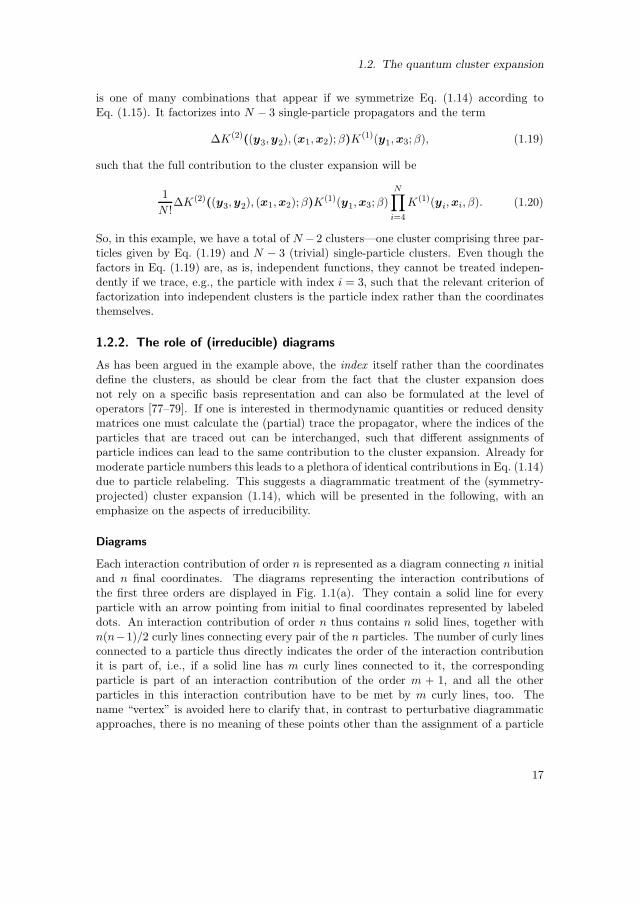
Diagrams
Each interaction contribution of order n is represented as a diagram connecting n initialand n final coordinates. The diagrams representing the interaction contributions ofthe first three orders are displayed in Fig. 1.1(a). They contain a solid line for everyparticle with an arrow pointing from initial to final coordinates represented by labeleddots. An interaction contribution of order n thus contains n solid lines, together withn(n−1)/2 curly lines connecting every pair of the n particles. The number of curly linesconnected to a particle thus directly indicates the order of the interaction contributionit is part of, i.e., if a solid line has m curly lines connected to it, the correspondingparticle is part of an interaction contribution of the order m + 1, and all the otherparticles in this interaction contribution have to be met by m curly lines, too. Thename “vertex” is avoided here to clarify that, in contrast to perturbative diagrammaticapproaches, there is no meaning of these points other than the assignment of a particle
17

1. Quantum cluster expansions in short-time approximation
Figure 1.1: (a) Diagrams representing ∆K(n)(y,x;β), Eq. (1.13), for n = 1, 2, 3. (b)Diagram representing the particular cluster Eq. (1.19) for x = y.
to a certain interaction contribution. Instead of using curly lines, one could give a labelto each particle line indicating its affiliation to an interaction contribution. However,by graphically connecting the respective particles, one can directly determine whether agiven diagram factorizes, i.e., it can be split into two diagrams without cutting any lines,or whether it is irreducible, i.e., it cannot be split up further. A full diagram representsa factorization into clusters according to Eq. (1.14) or its symmetry-projected equivalentand comprises several irreducible diagrams that represent single clusters.
The cycle structure is then either encoded in the indices of the final coordinates ascompared to the initial ones or, in the case of particles that have been traced out, bythe connection of the particle lines. By convention, each unlabeled bullet in a diagramstands for a coordinate that has been traced out. Such points have to connect two particlelines or, in the case of a one-cycle, a particle line with itself. Loose ends correspond tountraced particles with different initial and final coordinates, such that they always haveto come in pairs. As an example, the irreducible diagram corresponding to Eq. (1.19) fory = x and with x3 traced out is depicted in Fig. 1.1(b). In practice it is convenient toomit one-particle irreducible diagrams while stating the particle number of the (reduced)diagrams explicitly. As a diagram contains the full information on the cycle structureone is free to include the sign factors from exchange symmetry in the diagram values.Here, however, the convention is used that the value of a diagram is defined irrespectiveof the exchange symmetry and treat the sign factors as additional prefactors.
Let us now focus on diagrams that appear in the full trace of the cluster expansion, i.e.,the canonical partition function, with the purpose of counting only distinct diagrams,then provided with multiplicities and a sign factor that encodes the particle symmetry.Consider a full diagram in the expansion that is built out of l irreducible diagrams ofsizes n1 ≥ · · · ≥ nl. By distributing the particle indices among the irreducible diagramsin a different way one finds equivalent full diagrams. Therefore, the multiplicity of anysuch diagram contains the combinatorial factor
#NN =
1∏∞
ν=1mN(ν)!
N !∏l
i=1 ni!=
N !∏∞
ν=1mN(ν)!(ν!)mN(ν), (1.21)
where mN(ν) is the multiplicity of the number ν in N = n1, . . . , nl. It is the number ofpossible partitions of the set of the N particle indices into subsets of the sizes n1, . . . , nl.
18

1.2. The quantum cluster expansion
This holds irrespective of the structure of the irreducible diagrams, whereas an additionalfactor counts the number of ways to relabel the coordinates inside an irreducible diagramdepending on its structure. The index l for the length of N was only introduced to shortennotation and does not appear the second form of the combinatorial factor (1.21). If wecollect all full diagrams in the cluster expansion that factorize into irreducible diagramsof the sizes n1, . . . , nl their sum can be written as
(#N
N
)l∏
i=1
S(0)ni,±(β), (1.22)
where S(0)n,±(β) is the sum of all n-particle irreducible diagrams, including the multiplici-
ties from internal relabeling as well as the sign factors from symmetrization. The upperindex (k) with k ∈ N0 denotes the number of particles that are not traced over andwill be different from zero when thermal expectation values of operators, e.g., particledensities or n-point correlation functions are concerned. Using the above definitions thepartition function can be written in terms of the sums of irreducible clusters as
Z(N)± (β) =
1
N !
∑
N⊢N#N
N
∏
n∈NS(0)n,±(β). (1.23)
Note that, in contrast to Eqs. (1.14) and (1.18), the sum runs over the partitions ofthe number N instead of the partitions of the index set 1, . . . , N. To be precise, theexplicit form of Eq. (1.23) is given by
Z(N)± (β) =
1
N !
N∑
l=1
∑
n1≥···≥nl≥1∑l
i=1ni=N
#Nn1,...,nl
l∏
i=1
S(0)ni,±(β).
=N∑
l=1
1
l!
N∑
n1,...,nl=1∑l
i=1ni=N
l∏
i=1
S(0)ni,±ni!
(1.24)
In this form, the cluster expansion of the canonical partition function is organized in away that the first sum runs over the number l of irreducible clusters.
The central role of the irreducible diagrams S(0)n,± as building blocks of the theory is
better demonstrated when looking at the grand canonical partition function. As willbe shown in section 1.2.3, it is given exactly as the exponentiated sum of irreduciblediagrams, only weighted with a combinatorial factor and the fugacity z:
ZG(β, µ) = exp
( ∞∑
k=0
zk
k!S(0)k (β)
)
, z = eµβ . (1.25)
Here, the index for the symmetry class ± has been omitted to highlight the simple formof the result.
19

1. Quantum cluster expansions in short-time approximation
Figure 1.2: The sum of irreducible k-particle diagrams S(0)k for k = 1, 2, 3. Most of
the diagrams for k = 3 appear with multiplicities larger than 1. The first three dia-
grams in S(0)3,± include only the interaction contributions up to order 2, while the rest
accounts for all six possible permutations of the third-order interaction contribution.For noninteracting indistinguishable particles, only the first diagrams contribute, while
for distinguishable particles only the second diagram in S(0)2,± and the fourth diagram in
S(0)3,± contribute.
Before moving on to the implications of the combinatorial nature of the cluster ex-pansion, let us consider, as an example, the cluster expansion for three indistinguishableparticles. There are three different partitions of the particles with combinatorial factors
#31,1,1 = 1, #3
2,1 = 3, #33 = 1 (1.26)
so that the partition function is given by
Z(3)± =
1
3!
[(
S(0)1,±
)3+ 3S
(0)2,±S
(0)1,± + S
(0)3,±
]
, (1.27)
where the dependence on β has been omitted. The sums of the k-particle irreducible
diagrams S(0)k,± for k = 1, 2, 3 are shown in Fig. 1.2, also including the multiplicities of
the individual diagrams due to internal relabeling.
We are now left with the calculation of the multiplicities due to internal relabeling andthe sign factors from exchange symmetry. Let us exemplarily focus on the multiplicity
of the second diagram in S(0)3,±. It is built from one interaction contribution of order
two and one free propagation (order one). Choosing the interacting pair out of threeparticles already gives three possibilities corresponding to the Ursell decomposition, cf.,Eq. (1.11). Then, one of the interacting particles has to be linked to the free particleby a two-cycle. This can be achieved with two distinct exchange permutations, yieldingthe overall multiplicity of 6. In addition, the factor ±1 has to be introduced to accountfor the two-cycle. A detailed formal description of how the coefficients are determinedin general can be found in [61].
1.2.3. Partial traces, recurrence relations, and expectation values
The previous subsection has introduced the basic notation and the the very generalcombinatorial nature of the cluster expansion for the example of the canonical partitionfunction, i.e., the full trace of the (imaginary time) propagator. When dealing with
20
1.2. The quantum cluster expansion
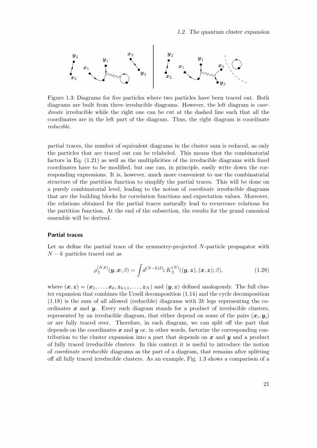
Figure 1.3: Diagrams for five particles where two particles have been traced out. Bothdiagrams are built from three irreducible diagrams. However, the left diagram is coor-
dinate irreducible while the right one can be cut at the dashed line such that all thecoordinates are in the left part of the diagram. Thus, the right diagram is coordinatereducible.
partial traces, the number of equivalent diagrams in the cluster sum is reduced, as onlythe particles that are traced out can be relabeled. This means that the combinatorialfactors in Eq. (1.21) as well as the multiplicities of the irreducible diagrams with fixedcoordinates have to be modified, but one can, in principle, easily write down the cor-responding expressions. It is, however, much more convenient to use the combinatorialstructure of the partition function to simplify the partial traces. This will be done ona purely combinatorial level, leading to the notion of coordinate irreducible diagramsthat are the building blocks for correlation functions and expectation values. Moreover,the relations obtained for the partial traces naturally lead to recurrence relations forthe partition function. At the end of the subsection, the results for the grand canonicalensemble will be derived.
Partial traces
Let us define the partial trace of the symmetry-projected N -particle propagator withN − k particles traced out as
ρ(N,k)± (y,x;β) =
∫
d(N−k)Dz K(N)± ((y,z), (x,z);β), (1.28)
where (x,z) = (x1, . . . ,xk,zk+1, . . . ,zN ) and (y,z) defined analogously. The full clus-ter expansion that combines the Ursell decomposition (1.14) and the cycle decomposition(1.18) is the sum of all allowed (reducible) diagrams with 2k legs representing the co-ordinates x and y. Every such diagram stands for a product of irreducible clusters,represented by an irreducible diagram, that either depend on some of the pairs (xi,yi)or are fully traced over. Therefore, in each diagram, we can split off the part thatdepends on the coordinates x and y or, in other words, factorize the corresponding con-tribution to the cluster expansion into a part that depends on x and y and a productof fully traced irreducible clusters. In this context it is useful to introduce the notionof coordinate irreducible diagrams as the part of a diagram, that remains after splittingoff all fully traced irreducible clusters. As an example, Fig. 1.3 shows a comparison of a
21

1. Quantum cluster expansions in short-time approximation
coordinate reducible and a coordinate irreducible diagram for five particles, where twoparticles have been traced out.
One can now proceed in the same way as in the previous subsection and define
A(k)n,±(x,y;β) as the sum of all coordinate irreducible diagrams composed of n parti-
cles. In every diagram that contributes to A(k)n,±(y,x;β), n − k particle coordinates are
traced out. The respective particle indices are drawn from the N − k coordinates thatare traced over, such that there are
(N − kn− k
)
=(N − k)!
(n− k)!(N − n)!(1.29)
equivalent diagrams in the overall sum. The remaining N − n particles will then bedistributed in all possible fully traced irreducible diagrams with their sum given by
(N − n)!Z(N−n)± , as seen in the last subsection. Thus, only by rearranging the cluster
expansion, we can write the partial trace (1.28) as
ρ(N,k)± (y,x;β) =
1
N !
N∑
n=k
(N − kn− k
)
A(k)n,±(y,x;β) · (N − n)!Z
(N−n)± (β)
=(N − k)!
N !
N∑
n=k
A(k)n,±(y,x;β)
(n− k!)Z
(N−n)± (β)
=(N − k)!
N !
N∑
n=k
a(k)n,±(y,x;β)Z
(N−n)± (β), (1.30)
where Z(0)± (β) = 1 by convention. In Eq. (1.30) the rescaled sum of coordinate irreducible
diagrams
a(k)n,±(y,x;β) =
A(k)n,±(y,x;β)
(n− k)!(1.31)
has been introduced. It is convenient to define also the rescaled sum of irreducibleclusters as
s(k)n,±(β) =
S(k)n,±(β)
(n− k − δk0)!(1.32)
where δkl is the Kronecker delta and the factorial is chosen such that it cancels theinternal multiplicity of the cyclic diagrams in the noninteracting case.
As the dependence on the inverse temperature β is clear from the definitions, it will bedropped in the following for better readability. Moreover, the label ± for the exchangesymmetry will be omitted.
For the cases k = 1 and k = 2 that will be of relevance later one obtains
a(1)n (y,x) = s(1)n (y,x), (1.33)
a(2)n (y,x) = s(2)n (y,x) +
n−1∑
l=1
s(1)l (y1,x1)s
(1)n−l(y2,x2). (1.34)
22

1.2. The quantum cluster expansion
With this notation the partial trace of the propagator for k = 1 and k = 2 is convenientlywritten as
ρ(N,1)(y,x) =1
N
N∑
n=1
s(1)n (y,x)Z(N−n), (1.35)
ρ(N,2)(y,x) =1
N(N − 1)
(N∑
n=2
s(2)n (y,x)Z(N−n)
+
N−1∑
k=1
N−k∑
l=1
s(1)k (y1,x1)s
(1)l (y2,x2)Z(N−k−l)
)
. (1.36)
Equations of this kind are of central relevance for the calculation of expectation values.However, they can also be used to derive recurrence relations as will be shown below.
Recurrence formulas
By tracing out the remaining particle in Eq. (1.35) one immediately finds the very usefulrecurrence relation for the canonical partition function
Z(N) =1
N
N∑
n=1
s(0)n Z(N−n) (1.37)
that has been long known for the noninteracting case [83]. It has also been used re-cently as a very useful tool in quantum Monte Carlo approaches [17] where the recursiveapproach drastically reduces the computational effort. Tracing Eq. (1.36) one finds adifferent recurrence relation
Z(N) =1
N(N − 1)
(N∑
n=2
(n− 1)s(0)n Z(N−n) +
N−1∑
k=1
N−k∑
l=1
s(0)k s
(0)l Z(N−k−l)
)
. (1.38)
More general, Eq. (1.30) yields a recursion formula for every k ≥ 1, but the resultingexpressions become, of course, more complicated with increasing k and their usefulnessfor practical purposes might become questionable. Nevertheless, if one wants to find
new recursion formulas, one should keep in mind that the functions s(k)n are related to
each other by
∫
dDxk+1 s(k+1)n ((y,xk+1), (x,xk+1)) = (n− k)s(k)n (y, x) (1.39)
for k > 0. Here, x denotes the k remaining coordinates x1, . . . ,xk. For k = 0 one simplyhas ∫
dDx s(1)n (x,x) = s(0)n . (1.40)
23

1. Quantum cluster expansions in short-time approximation
Expectation values
The relations for the partial traces are of use when one is interested in the thermalexpectation value
〈O〉β =1
Z(N)±
Tr(N)±[
e−βHO]
(1.41)
of an observable O, where the trace is taken in the Hilbert space sector with bosonic (+)or fermionic symmetry (−). Let us start with the simple case of a one-particle observable
O1 =
N∑
i=1
O(i)1 =
∫
dDx dDyO1(x,y)ψ†(x)ψ(y), (1.42)
where O1(x,y) = 〈x|O1|y〉 and ψ† and ψ are the bosonic or fermionic field operators.The thermal expectation value of A is then given by
〈O1〉β =
∫
dDx dDyO1(x,y)〈ψ†(x)ψ(y)〉β (1.43)
in terms of the single-particle reduced density matrix or two-point correlation function
〈ψ†(x)ψ(y)〉β =1
Z(N)± (β)
Tr(N)±[
e−βH ψ†(x)ψ(y)]
=Nρ
(N,1)± (y,x;β)
Z(N)± (β)
. (1.44)
The last identity will be shown below in a more general context. Using Eq. (1.35) for
ρ(N,1)± then yields, dropping the β-dependence,
〈ψ†(x)ψ(y)〉β =1
Z(N)±
N∑
n=1
s(1)n (y,x)Z(N−n)± . (1.45)
So, to calculate the expectation values of one-particle operators, one only needs the
additional information of the irreducible clusters s(1)n . This can be extended to arbitrary
k-particle operators. In general, the expectation value of the normal ordered product offield operators is given by
C(N,k)± (y,x) = 〈Ψ†(x1) · · · Ψ†(xk)Ψ(yk) · · · Ψ(y1)〉β (1.46)
=N !
(N − k)!
ρ(N,k)± ((y1, . . .yk), (x1, . . . ,xk);β)
Z(N)±
, (1.47)
as is shown in appendix A. Note the reversed order of the coordinates yi in (1.46) thatis important in the case of fermions. Finally, by making use of Eq. (1.30) one obtainsthe simple result
C(N,k)± (y,x) =
1
Z(N)±
N∑
n=k
a(k)n,±(y,x)Z
(N−n)± . (1.48)
24

1.2. The quantum cluster expansion
The expectation value of a k-particle operator
Ok =
N∑
i1,...,ik=1ij 6=il
O(i1,...,ik)k (1.49)
in the canonical ensemble is thus given by
〈Ok〉β =
∫
dkDx dkDyOk(x,y)C(N,k)± (y,x;β), (1.50)
where the dependence on β has been restored and Ok(x,y) is the matrix element
Ok(x,y) = 〈x|O(1,...,k)k |y〉 , (1.51)
that is calculated in a k-particle subspace of the N -particle Hilbert space. Note thataccording to Eq. (1.48) the expectation value (1.50) is expressed only using the coordinateirreducible clusters and the canonical partition functions of subsystems.
The grand canonical ensemble
We have seen that the canonical partition function is completely determined by irre-ducible clusters via recursive formulas. Moreover, correlation functions and thus the ex-pectation values they generate are completely determined by the coordinate irreduciblediagrams and the irreducible clusters that enter the partition function. This again high-lights the fact that, if the (coordinate) irreducible clusters are known, the calculation ofthe full cluster expansions is merely a combinatorial problem. The latter originates fromthe fact that the particle number N is fixed exactly in the canonical formalism. This con-dition is relaxed in the grand canonical ensemble, leading to a description that dependsonly on the (coordinate) irreducible diagrams while not suffering from any combinatorialdifficulties.
The grand canonical partition function can be expressed through the canonical parti-tion function as
ZG± (β, µ) =
∞∑
N=0
zNZ(N)± (β), (1.52)
where z = eβµ is the fugacity and µ is the chemical potential that controls the aver-age number of particles in the system. The logarithmic derivative of Eq. (1.52) withrespect to the fugacity is given by (omitting the index for the particle symmetry and thefunctional dependencies for the rest of this subsection)
∂
∂zlogZG =
1
ZG
∞∑
N=1
zN−1NZ(N) =1
ZG
∞∑
N=1
zN−1N∑
k=1
s(0)k Z(N−k)
=1
ZG
( ∞∑
m=1
zm−1s(0)m
)( ∞∑
n=0
znZ(n)
)
︸ ︷︷ ︸
ZG
=
∞∑
m=1
zm−1s(0)m , (1.53)
25
1. Quantum cluster expansions in short-time approximation
where the recurrence relation (1.37) for Z(N) and the Cauchy product formula have beenused (assuming convergence of the series). Using ZG|z=0 = Z(0) = 1 one immediatelygets
ZG = exp
( ∞∑
m=1
zm
ms(0)m
)
, (1.54)
such that the grand potential Ω is given by the sum of irreducible clusters,
Ω(β, µ) = − 1
βlogZG = − 1
β
∞∑
m=1
zm
ms(0)m . (1.55)
For the correlation functions let us first relate the expectation values in the two ensem-bles:
〈Ok〉β,µ =1
ZGTr[
e−β(H−µN)Ok
]
=1
ZG
∞∑
N=0
zN Tr(N)[
e−βHOk
]
=1
ZG
∞∑
N=0
zNZ(N)〈Ok〉β . (1.56)
Here, the first trace is over the full Fock space. Using Eq. (1.48) one finds
C(k)(y,x, β, µ) = 〈Ψ†(x1) · · · Ψ†(xk)Ψ(yk) · · · Ψ(y1)〉β,µ
=1
ZG
∞∑
N=k
zNZ(N)C(k,N)(y,x, β)
=1
ZG
∞∑
N=k
zNN∑
l=k
a(k)l (y,x)Z(N−l)
=1
ZG
( ∞∑
n=k
zna(k)n (y,x)
)( ∞∑
m=0
zmZ(m)
)
︸ ︷︷ ︸
ZG
=
∞∑
n=k
zna(k)n (y,x). (1.57)
This means that the thermal expectation values are directly determined by the coordi-nate irreducible diagrams. This is in analogy to the cancellation of vacuum bubbles inquantum field theories. The interpretation is, however, different, as there are no vacuumbubbles in a particle-conserving theory. It is rather the statistical average over systemswith different particle numbers that leads to the simplifications in the grand canonicalensemble. Another way to view the simple expressions obtained in the grand canonicalensemble is to simply take them as the generating functions of the canonical partition
26

1.2. The quantum cluster expansion
function and expectation values via
Z(N) =1
N !
[∂N
∂zNZG
]
z=0
, (1.58)
〈O〉β =1
N !Z(N)
[∂N
∂zN
(
ZG〈O〉β,µ)]
z=0
. (1.59)
1.2.4. Generalization to multiple species
In this subsection, the generalizations of the previous results for multiple species isprovided. This is of relevance not only in mixtures of fundamentally distinguishableparticles but also in systems where single-particle degrees of freedom are conserved bythe inter-particle interaction, thus making the particles effectively distinguishable. Themost important examples comprise the cases of spin-1/2 fermions with spin-conservinginteractions and composite particles with internal degrees of freedom that are robustagainst collisions.
The results of the previous sections are straightforwardly generalized using multi-indexnotation
n = (n1, . . . , nl), n! =l∏
i=1
ni!, en = (en1 , . . . , enl), (1.60)
zn =l∏
i=1
zni
i , ∂n =l∏
i0
∂ni
i ,N∑
n=k
=
l∏
i=1
Ni∑
ni=ki
, (1.61)
where l is the number of species. Let us denote the coordinates of theNi indistinguishable
particles of species i as Xi = (x(i)1 , . . . ,x
(i)Ni
) and the coordinates of all particles by
X. Using the many-body imaginary-time propagator K(N)(Y ,X;β) for N1 + · · · +Nl
particles, the symmetry-projected propagator is generalized from (1.15) to
K(N)σ (Y ,X;β) =
1
N !
∑
P∈SN
σPK(N)(PY ,X ;β), (1.62)
where the sum runs over all tuples (P (1), . . . , P (l)) ∈ SN = SN1 × · · · × SNland the
individual permutations act only on the coordinates of the respective particle speciesPY = (P (1)Y (1), . . . , P (l)Y (l)). The exchange symmetry in each particle species isencoded in the indices σi = ±1 for i = 1, . . . , l. With the same notation, the sums of
(coordinate) irreducible clusters S(k)n,σ(Y ,X ;β) and A
(k)n,σ(Y ,X ;β) can be introduced,
with the same definitions of irreducibility as before. Here, the multi-indices n and k
have to fulfill n ≥ k and k > 0 in A(k)n , making use of the partial order that can be
defined bys ≥ t ⇔ si ≥ ti for all i = 1, . . . , l. (1.63)
Note that as before, abusing notation, the arguments X and Y in S(k)n,σ and A
(k)n,σ are
defined by the tuple k in that they contain kj particle coordinates of the species j (kj = 0
27
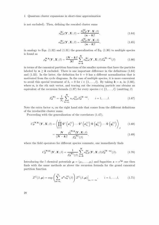
1. Quantum cluster expansions in short-time approximation
is not excluded). Then, defining the rescaled cluster sums
s(k)n,σ(Y ,X ;β) =
S(k)n,σ(Y ,X ;β)
(n − k)!, (1.64)
a(k)n,σ(Y ,X ;β) =
A(k)n,σ(Y ,X;β)
(n− k)!, (1.65)
in analogy to Eqs. (1.32) and (1.31) the generalization of Eq. (1.30) to multiple speciesis found as
ρN ,kσ (Y ,X ;β) =
(N − k)!
N !
N∑
n=k
a(k)n,σ(Y ,X;β)Z
(N−n)σ (β) (1.66)
in terms of the canonical partition functions of the smaller systems that have the particleslabeled by n ≥ k excluded. There is one important difference in the definitions (1.64)and (1.32). In the latter, the definition for k = 0 has a different normalization that ismotivated from the cycle diagrams. In the case of multiple species, it is more convenientto avoid this special treatment of ki = 0 for i ∈ 1, . . . , l. By taking k = ei in (1.66),where ei is the ith unit vector, and tracing out the remaining particle one obtains anequivalent of the recursion formula (1.37) for every species i ∈ 1, . . . , l (omitting β)
Z(N)σ =
1
Ni
N∑
n=ei
nis(0)n,σZ
(N−n)σ , i = 1, . . . , l. (1.67)
Note the extra factor ni on the right hand side that comes from the different definitionsof the irreducible cluster sums.
Proceeding with the generalization of the correlators (1.47),
C(N ,k)σ (Y ,X;β) =
⟨l∏
i=1
Ψ†(
x(i)1
)
· · · Ψ†(
x(i)ki
)
Ψ(
y(i)ki
)
· · · Ψ(
y(i)1
)⟩
β
(1.68)
=N
(N − k)!
ρ(N ,kσ (Y ,X ;β)
Z(N)σ (β)
, (1.69)
where the field operators for different species commute, one immediately finds
C(N ,k)σ (Y ,X ;β) =
1
Z(N)σ (β)
N∑
n=k
a(k)n,σ(Y ,X;β)Z
(N−n)σ (β). (1.70)
Introducing the l chemical potentials µ = (µ1, . . . , µl) and fugacities z = eβµ one thenfinds with the same methods as above the recursion formula for the grand canonicalpartition function
ZG(β,µ) = exp
( ∞∑
n=ei
zns(0)n (β)
)
ZG(β,µ)∣∣∣µi→−∞
, i = 1, . . . , l, (1.71)
28

1.2. The quantum cluster expansion
where the last factor is the grand partition function without species i. It is easily provenby taking logarithmic derivatives of ZG with respect to the fugacities. The full result isthe generalization of (1.54),
ZG(β,µ) = exp
( ∞∑
n=0
zks(0)n (β)
)
. (1.72)
Finally, the generalization of Eq. (1.57) can be given as
C(k)(Y ,X;β,µ) =∞∑
n=k
zna(k)n (Y ,X , β). (1.73)
As before, they are sufficient to calculate the expectation value of any k-particle observ-able.
1.2.5. Resummation of clusters
In this section, the important case of systems that are homogeneous in space is con-sidered. In such systems, the total momentum is conserved, such that the many-bodypropagator in momentum space is diagonal in the total momentum. Moreover, tracingout one particle fixes the initial and final momentum of the respective particle to be thesame, such that the total momentum of the remaining particles must be conserved. This
means that the n-point correlation functions C(N,k)± (y,x), Eq. (1.48), and C
(k)± (y,x),
Eq. (1.57), are diagonal in the total momentum of the k particles that are not tracedover. This does also apply to individual diagrams in the cluster expansion, and thusany coordinate irreducible diagram. In this section we will only focus on the reducedone-body density matrix, i.e., all but one particles are traced out. In this case one has
a(1)n,± = s
(1)n,± and this sum of irreducible diagrams can then be written in the as
s(1)n,±(y,x) = s
(1)n,±(y − x, 0) =
1
(2π)D
∫
dDk eik(y−x)s(1)n,±(k), (1.74)
with the momentum representation of the irreducible cluster sums
s(1)n,±(k) =
∫
dDz e−ikzs(1)n,±(z, 0). (1.75)
The reduced one-body density matrix in momentum representation is thus diagonal and,using Eq. (1.57), given by
C(1)± (k) =
∫
dDz e−ikzC(1)± (y − x, 0) =
∞∑
n=1
zns(1)n,±(k). (1.76)
Up to this point one has not gained much from the representation in momentum space.However one should note that many irreducible diagrams now factorize. To be more
specific, if a two-legged irreducible diagram in s(1)n,± can be cut into two pieces such that
29

1. Quantum cluster expansions in short-time approximation
Figure 1.4: The factorization of diagrams in the reduced one-body density matrix. Thediagram on the left can be cut into two pieces at the dashed line, and it has the samemomentum k at this point. The value of the full diagram is then the product of the twodiagrams evaluated at the same momentum k. As cutting the diagram is achieved byinterchanging two particle indices, one has to account for the exchange symmetry witha factor ±1.
one ends up with two new two-legged diagrams, the full diagram is given by the productof the latter. Figure 1.4 shows an example of such a factorization. There, insteadof labeling the initial and final coordinates, the momentum k is used and the signfactors from exchange symmetry have been included in the diagram values for simplicity(opposing the convention introduced in section 1.2.2), leading to the sign factor on theright hand side, as, on a formal level, any two-legged diagram that can be cut in theabove manner is linked by a single exchange of particle indices. This can be seen asfollows: Let (±1)PaDa and (±1)PbDb be the disconnected parts of the diagram and(±1)PabDab the connected diagram, i.e., Pa, Pb, and Pab are the permutations that enterthe diagrams and Pa and Pb act on disjoint sets of particle indices. Let P = (12) theexchange permutation of the indices 1 and 2, then
Dab(y1,x1) =
∫
dDx2Db(y1,x2)Da(x2,x1)
=
∫
dDx2 dDy2 δ
(D)(x2 − y2)Db(y1,x2)Da(y2,x1)
=
∫
dDx2 dDy2 δ
(D)(x2 − y2)Db(yP (2),x2)Da(yP (1),x1), (1.77)
such that in the connected diagram one has to account for the the additional particleexchange P as compared with the disconnected parts, giving rise to a factor (±)P = ±1for each cut. To be precise, the cycle structure of the connected diagram is given byPab = P Pa Pb and the sign factor is given by
(±1)Pab = (±1)PPaPb = ±(±1)PaPb = ±(±1)Pa(±1)Pb . (1.78)
As was explained in section 1.2.2, each irreducible diagram has a certain internalmultiplicity due to possible relabeling of the particles that have been traced out. Tomake use of the factorization of diagrams we need to explore how the multiplicity of thefull diagram is related to the multiplicities of the constituents. This can be done on apurely combinatorial level. Let us assume that we have a two-legged irreducible diagramof n = k + l particles that can be cut into two such diagrams with k and l particles,
30
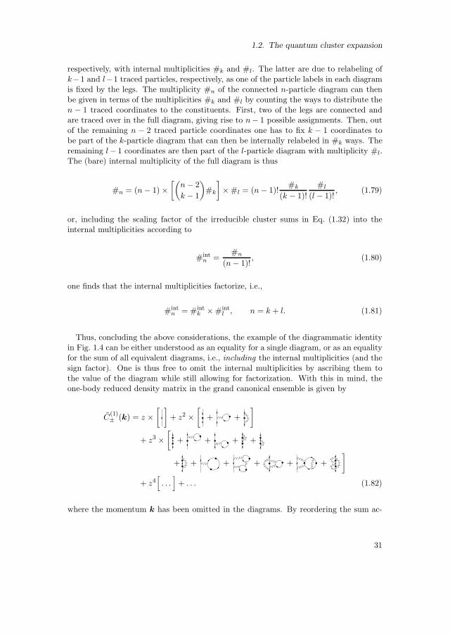
1.2. The quantum cluster expansion
respectively, with internal multiplicities #k and #l. The latter are due to relabeling ofk−1 and l−1 traced particles, respectively, as one of the particle labels in each diagramis fixed by the legs. The multiplicity #n of the connected n-particle diagram can thenbe given in terms of the multiplicities #k and #l by counting the ways to distribute then − 1 traced coordinates to the constituents. First, two of the legs are connected andare traced over in the full diagram, giving rise to n− 1 possible assignments. Then, outof the remaining n − 2 traced particle coordinates one has to fix k − 1 coordinates tobe part of the k-particle diagram that can then be internally relabeled in #k ways. Theremaining l− 1 coordinates are then part of the l-particle diagram with multiplicity #l.The (bare) internal multiplicity of the full diagram is thus
#n = (n− 1) ×[(n− 2
k − 1
)
#k
]
× #l = (n− 1)!#k
(k − 1)!
#l
(l − 1)!, (1.79)
or, including the scaling factor of the irreducible cluster sums in Eq. (1.32) into theinternal multiplicities according to
#intn =
#n
(n− 1)!, (1.80)
one finds that the internal multiplicities factorize, i.e.,
#intn = #int
k × #intl , n = k + l. (1.81)
Thus, concluding the above considerations, the example of the diagrammatic identityin Fig. 1.4 can be either understood as an equality for a single diagram, or as an equalityfor the sum of all equivalent diagrams, i.e., including the internal multiplicities (and thesign factor). One is thus free to omit the internal multiplicities by ascribing them tothe value of the diagram while still allowing for factorization. With this in mind, theone-body reduced density matrix in the grand canonical ensemble is given by
C(1)± (k) = z ×
[ ]
+ z2 ×[
+ +
]
+ z3 ×[
+ + + +
+ + + + + +
]
+ z4[
. . .]
+ . . . (1.82)
where the momentum k has been omitted in the diagrams. By reordering the sum ac-
31

1. Quantum cluster expansions in short-time approximation
cording to the number of factors in the diagrams one obtains the formal power expansion
C(1)± (k) = z ×
[
+ z ×(
+
)
+ z2(
+ . . .
)
+ . . .
]
± z2 ×[
+ z ×(
+
)
+ z2(
+ . . .
)
+ . . .
]2
+ z3 ×[
+ z ×(
+
)
+ z2(
+ . . .
)
+ . . .
]3
+ . . . . (1.83)
Thus, the full expansion can be reordered to a formal power series in the dressed Boltz-mann factor
c±(k) = = + z ×(
+
)
+ z2(
+ . . .
)
+ . . . (1.84)
that contains only diagrams that cannot be cut anymore. Note, again, that the signfactors for the exchange symmetry are included in the diagrams here, opposing theconvention of other sections. The one-body reduced density matrix can thus be formallywritten as
C(1)± (k) = ±
∞∑
n=1
[±zc±(k)]n =zc±(k)
1 ∓ zc±(k)=
1
[zc±(k)]−1 ∓ 1. (1.85)
This has the form of the Bose-Einstein (upper sign) or Fermi distributions (lower sign) forthe occupation of the single-particle states with momentum k, but with the Boltzmannfactor replaced by the dressed function c±(k). In the case of vanishing interactions onehas c±(k) → e−βE(k) with E(k) = ~
2k2/2m such that the correct noninteracting resultfor the one-particle density matrix is obtained:
C(1)± (k)
NI−→ 1
eβ(Ek−µ) ∓ 1. (1.86)
Although there is no guarantee that the dressed Boltzmann factor has a positive conver-gence radius for finite interaction, it could give much better asymptotic approximationsthan other approaches. One reason for this is the fact that even for free fermions, where
s(1)n,−(k) = (−1)n−1e−nβEk , (1.87)
the fugacity expansion (1.76) does not converge for z e−βEk ≥ 1, i.e., Ek ≤ µ ∼ EF, aregime that is, however, covered by the Fermi function (1.86) being the analytic contin-uation of the series expression.
A natural application of Eq. (1.85) is a perturbative expansion
− 1
βlog (zc±(k)) = Ek − µ+ b1γ + O(α2) (1.88)
32

1.2. The quantum cluster expansion
in a small coupling γ to obtain a mean field description in terms of a shifted single-particle energy. A more elaborate way to proceed could be a recursive calculation of thedressed Boltzmann factor c± by noting that it has a self similar structure. For example,one can generate a whole class of diagrams that only contain interaction contributionsof second order by truncating the series expansion of c±(k) after the linear term, whilereplacing the single dot in each diagram by the rule
• 7→ 1 ± C(1)± (k′) =
[1 ∓ zc±(k′)
]−1(1.89)
before integrating over the momentum k′. To be specific, one would obtain an integralequation of the form
c±(k) = e−βEk + z
∫
dDk′f(k,k′)
1 ± zc±(k′), (1.90)
with the function f being defined by the diagonal and exchange elements of the inter-action contribution ∆K(2) in momentum space. Extensions that generate a larger classof diagrams are also possible. Although all the ingredients are available, e.g., for shortrange interactions in arbitrary dimensions [84], this approach has not been taken yetand might be subject of a future project.
33

1. Quantum cluster expansions in short-time approximation
1.3. Short times—smooth spectra—high temperatures
The previous section has introduced the cluster expansion on a purely formal level,being valid for any kind of systems with fixed number of particles. However, despitethe conceptually simple formulas that one obtains in the theory, one still has to face thefact that, in almost all situations, only the simplest diagrams can be exactly calculated.Moreover, if a finite system is considered, the values of irreducible diagrams are notindependent of the external potentials or the system’s boundaries. Therefore, this sectionis dedicated to the introduction of certain approximations that help solving some of thesedifficulties.
The section is structured as follows: First, using the analogy of short-time propagationand high-temperature quantum statistics, the general short-time scaling of the quantumcluster expansion is reviewed, also introducing the (smooth) density of states that definesthe microcanonical ensemble. Then, the scaling is used for the analytical treatment of acertain class of diagrams that can be calculated whenever the interaction contributionsof second order are known explicitly, being of use for later sections. Finally, after theimplications of the high temperature scaling on the thermodynamic limit is put forward,a self-consistent method for calculating the mean energy shifts due to interaction isreviewed, with a focus on its scaling in the thermodynamic limit.
1.3.1. Short-time propagation and high-temperature scaling
This subsection gives an overview of the short-time approximation and the general di-mensional scaling properties of propagators that were introduced in [52, 61, 85]. Forfurther details, the reader is referred to the literature.
The starting point for the quantum cluster expansion was the many-body propagator.However, as was noted before, the whole theory is basis-independent and can even beformulated at the level of operators. The reason for using the (imaginary time) prop-agator is that it is very well understood at the level of single-particle systems, wherea saddle point approximation in the Feynman path integral leads to the semiclassicalVan Vleck-Gutzwiller propagator [41, 49], that comes as a sum over classical paths andadmits a systematic approximation for short times. In the context of billiard systems,the short-time approximation, that takes only into account the shortest classical paths,plays a special role as it contains the information on the smooth part of density of states,then given by Weyl’s law and the Weyl expansion [49,50].
Now, a key step is to realize that if the temperature is large enough, the discreteness ofthe many-body spectrum becomes unimportant due to its high level density. This has tobe contrasted to the assumption of a smooth single-particle level density, as the latter is,e.g., not capable of describing Bose-Einstein condensation in bosonic systems unless thesingle-particle ground state is treated separately [13]. A many-body description does notsuffer from any such problems. Therefore, the discreteness of the many-body DOS can beneglected even for temperatures inside the quantum degenerate regime or in the presenceof condensation effects as long as the number of uncondensed particles is not very small.It is then sufficient to include only the short-time information on the propagators G(N)
34

1.3. Short times—smooth spectra—high temperatures
to be specified in the following. For finite systems without external potentials all thepropagators in the calculation are replaced by their infinite space equivalents, i.e., it isassumed that the particles do not explore the whole system in arbitrarily short times.Formally, this corresponds to only taking into account the shortest classical paths in theVan Vleck-Gutzwiller propagator. The condition for this approximation to be accuratecan be estimated at the single-particle level to be
t≪ mV2D
2π~≡ tT, (1.91)
where m is the mass of the particle, V is the volume of the system, and D is thedimension. The characteristic time tT can be thought of as the typical traversal timethrough the system of a particle with momentum ~V −1/D, where the latter correspondsto the minimal uncertainty in the momentum of a wave packet in the volume V . If weswitch to imaginary time the condition (1.91) can be translated into
λDT ≪ V, (1.92)
introducing the thermal (de Broglie) wavelength
λT =
√
2π~2β
m. (1.93)
At this length scale the propagator of a single free particle decays in imaginary timet = −i~β. This gives the intuitive picture that within the regime of validity of the short-time approximation all clusters of particles have a characteristic size that scales with λTthat is much smaller than any length scale introduced from external confinement, suchthat their internal structure is essentially independent of the latter. It is worth stressingthat the short-time approximation does not require that the thermal wavelength is smallcompared to the mean inter-particle separation, i.e., one can have
NλDTV
> 1, (1.94)
in contrast to the case of high-temperature expansions in the thermodynamic limit. Thisparameter will also be referred to as the “quantum degeneracy parameter” later, as itmarks the onset of dominant quantum effects. For example, BEC sets in at Nλ3T /V =ζ(3/2) ≈ 2.61 in three dimensions [13]. The term “quantum degenerate regime” will beused when NλDT /V is of order one or larger and will thus refer to both fermionic andbosonic gases.
As the short-time approximation specified above is obtained from taking the short-est paths in the Van Vleck-Gutzwiller propagator, it can be easily extended to include,e.g., corrections from boundaries that improve the range of applicability to even smallertemperatures and energies. The short-time approximation of the propagator therebyencodes the information on the slowly varying parts of the density of states: The boundin Eq. (1.91) plays the role of a Heisenberg time tH = 2π~/∆ where ∆ is the mean single-particle level spacing2. It can be understood as a lower bound for the time needed to
2Estimated around the ground state using Weyl’s law for the smooth density of states.
35

1. Quantum cluster expansions in short-time approximation
resolve the discreteness of the spectrum. This means that the price we pay for using theshort-time approximation is the loss of all information related to this discreteness. How-ever, as the levels in noninteracting many-particle systems can be estimated to becomeexponentially dense in a certain window not very high in energy [86], the knowledge ofthe exact position of individual levels is only important very close to the ground state.
In the presence of smooth external potentials the short-time approximation can bemodified such that only the internal dynamics of a cluster is mapped to infinite space,while its center of mass evolves according to the single-particle (short-time) propagator[60, 85]. This assumes that the spatial extent of a cluster is small compared to thevariations of the external potential, which is justified by the short-range character ofthe interactions together with the short-time approximation. However, to be consistentwith the latter, the external potential has to be included only as a phase factor, hereevaluated in imaginary time,
K(n)clust(y,x;β) ≈ K
(n)clust(y,x;β)
∣∣∣Vext=0
× e−β∫ 10 ds
∑ni=1 Vext((yi−xi)s+xi) (1.95)
that can be found from the Eikonal approximation [61]. The function K(n)clust Eq. (1.95)
represents any irreducible cluster.The power of the short-time approximation lies in the high level of generality, leading
to certain general scaling properties. Let us first focus on the full trace of a cluster asit appears, e.g., in the partition function. As the internal cluster dynamics is treatedlike in homogeneous systems in the short-time approximation, it is invariant with re-spect to a translation of all the coordinates. Without external potentials this invariantdirection leads to a factor in the full trace that is proportional to the volume of thesystem, while in the case of slowly varying external potentials, their effect can be ap-proximated by evaluating Eq. (1.95) at the point where all coordinates coincide, leadingto a contribution
∫
d(N−1)DxK(n)clust(x,x;β)
∣∣∣x1=0,Vext=0
×∫
dDx1 exp (−βnVext(x1)) (1.96)
of the respective cluster to the partition function, where the first term is calculatedindependently of the external potential3. Similar approximations can be applied forpartial traces, where x1 should be one of the untraced coordinates or the center of mass.
Before further analyzing the short-time dynamics it is instructive to review the generaldimensional scaling [61,85] of the exact non-relativistic propagators, only assuming thatthe form of the Hamiltonian in position representation is given in the standard form
H =
Dtot∑
i=1
− ~2
2mii + V (x), (1.97)
where V (x) is a function that only depends on the Dtot coordinates x, an energy scaleα, a reference mass m and Planck’s constant, together with an arbitrary number of
3In the cluster expansion of the grand potential, i.e., for the fully traced clusters, this approximation isclosely related to a local density approximation [87,88], but should be considered more general whenapplied to propagators and partial traces.
36

1.3. Short times—smooth spectra—high temperatures
dimensionless parameters λ that encode, e.g., the mass ratios and different length scales.Explicitly, the potential has to be of the form
V = V (x;α,m, ~,λ). (1.98)
The latter assumption actually encodes the restriction that the potential should becompletely determined by ~ and quantities that can either be expressed in the SI units oftime, mass, and length, or can be combined to have the latter units, which is the genericsituation. This means that the strongest assumption in the form of the Hamiltonian(1.97) lies in the homogeneity of degree −2 of the kinetic energy.
With the above assumptions one can show [85] that the (imaginary time) propagatorcan be generally written as
K(y,x;β, α,m, ~,λ) =1
λDtotT
k
(y
λT,x
λT;βα,λ
)
(1.99)
with a dimensionless function k that depends only on dimensionless quantities.The potential V in (1.98) is usually the sum of external and interaction potentials with
their interplay encoded in the dimensionless parameters λ. However, in the short-timeapproximation the internal cluster dynamics is assumed to decouple from the externalpotential, such that the scaling can be applied to the interactions separately. Thus,assuming an interaction potential V of the form (1.98) one can rewrite the contributionof the internal dynamics of the irreducible clusters (1.95) as
K(n)clust(y,x;β)
∣∣∣Vext=0
=1
λnDTk(n)clust
(y
λT,x
λT;βα
)
(1.100)
as a dimensionless function k(n)clust that is invariant under the translation of all coordinates.
Approximating the external potential by evaluating all the coordinates at the same pointz then leads to
K(n)clust(y,x;β) ≈ 1
λnDTk(n)clust
(y
λT,x
λT;βα
)
e−nβVext(z). (1.101)
Here, z corresponds to the invariant direction of k(n)clust and can be understood as the
center of mass position of the cluster, but in practice any of the xi or yi can be used.Then, however, one has to keep in mind that the coordinate z should not be traced overin any partial traces. By further assuming the form (1.98) also for the external potentialone may write it as
Vext(z) = αextvext
(√
αextβz
λT
)
, (1.102)
where αext is the energy scale and possible dimensionless parameters λext have beensuppressed.
Equation (1.101) implies very generally that in the short-time approximation the func-
tions s(k)n in Eq. (1.32) factorize into λ−kD
T and a function of s = αβ for k > 0. For
37
1. Quantum cluster expansions in short-time approximation
k = 0, homogeneous potentials allow for further direct analysis: If the external potentialis homogeneous of degree η, i.e., vext(λx) = ληvext(x), the z-integration yields
1
λDT
∫
dDz e−nβαextvext
(√αextβ
zλT
)
= nD−d
2Veff
λdT, (1.103)
using the effective volume and dimension
Veff =
(2π~
mαext
)Dη∫
dDq evext(q), d = D
(
1 +2
η
)
. (1.104)
This also includes the case without external potential by taking η = ∞. To make thefactorization explicit let us define the dimensionless functions
b(k)n,±(y, x; s) = λkDT s
(k)n,±(y,x, β, α) for k > 0,
b(0)n,±(s) =
λdTVeff
s(0)n,±(β, α), (1.105)
that only depend on the rescaled coordinates x = x/λT and s = αβ. Note that the func-
tions b(0)n,± depend on the physical dimension D intrinsically and the effective dimension
d through the factor n(D−d)/2 in (1.103), i.e., they are of the form
b(0)n,±(s) = n
D−d2 b
(0)n,±(s)
∣∣∣vext=0
. (1.106)
1.3.2. The smooth density of states/microcanonical ensemble
As has been mentioned in the previous section, the discrete spectra of finite quantumsystems are approximated by smooth functions in the short-time approximation. To beprecise, the density of states (DOS) of the many-body quantum system, that is definedas
ρ(N)(E) =
∞∑
k=0
δ(
E − E(N)k
)
(1.107)
with the discrete N -particle energies E(N)k , is replaced by a smooth function ρ(N)(E).
Moreover, due to the scaling properties of the short-time approximation, it has a veryspecific dependence on the energy-like interaction parameter α. By collecting all contri-butions that have the same number of irreducible clusters one can write the full partitionfunction as a polynomial in the effective volume in units of the thermal wave length as [61]
Z(N,d)± (β) =
N∑
l=1
[
z(N,d)l,± + ∆z
(N,d)l,± (βα)
](Veff
λdT
)l
, (1.108)
where, following the notation in [61], the noninteracting clusters have been split off andthe dependence on the (effective) dimension has been made explicit. The coefficients
38

1.3. Short times—smooth spectra—high temperatures
in (1.108) can be read off from Eq. (1.24) as
[
z(N,d)l,± + ∆z
(N,d)l,± (s)
]
=1
l!
∑
n1,...,nl∑l
i=1ni=N
l∏
i=1
b(0)ni,±(s)
ni, (1.109)
where the dimensionless cluster sums defined in (1.105) have been used. For the nonin-
teracting case, where b(0)n,± = n−d/2, this was first reported in [89], where also recursion
relations for a fast calculation are provided.By using the general relation between the canonical partition function and the density
of states via the (both-sided) Laplace transformation
Z(β) = LE[ρ(E)](β) =
∫
dE e−βEρ(E), (1.110)
one can readily show that the integrated DOS, or level counting function
N (E) =
∫ E
−∞dE′ ρ(E′) (1.111)
is given by [60]
N (N,d)(E) =
N∑
l=1
z(N,d)l,± θ(E)
Γ( ld2 + 1)+ g
(N,d)l,± (E/α)
(ρeff0 E)ld2 , (1.112)
whereg(N,d)l,± (ǫ) = ǫ−
ld2 L−1
s
[
∆z(N,d)l,± (s)s−
ld2−1]
(ǫ) (1.113)
and
ρeff0 =mV
2d
eff
2π~2. (1.114)
Again, the interaction parameter α appears in a very specific way due to the assumptionsof the short-time approximation, i.e., the polynomial form of the smooth density of statesis not altered by the interaction, that only enters the coefficients (if E and E/α areconsidered as independent variables).
The smooth DOS is, of course, an important quantity by itself, as it contains a lot ofinformation about the actual (discrete) spectrum. It has, however, also a direct appli-cation as an ingredient for the microcanonical ensemble. The microcanonical partitionfunction M(E) counts the number of states in a small energy interval ∆ [62],
M(E) = N (E + ∆) −N (E). (1.115)
The nature of the interval ∆ is thereby such that the partition function M(E) should beinsensitive to small variations of the energy while its value should be sufficiently smallto allow one to consider the system as having a fixed energy. It thus plays the role of
39

1. Quantum cluster expansions in short-time approximation
smoothing the level distribution, so that, if we use the smooth counting function, onecan write M(E) as
M(E) = ρ(E)∆, (1.116)
such that it is actually smooth in the energy. This leads to the definition of the entropyas
S(E) = kB log ρ(E)∆ (1.117)
relevant for the thermodynamic properties of the system.
1.3.3. The QCE(n)—general results
As has been seen up to this point, the short-time approximation, applied to the dynamicsof individual clusters, allows one to separate the effects from external potentials andconfinement from the interaction contributions, such that the irreducible diagrams haveto be calculated only once and can then be used in different systems, giving rise toeffective dimension and volume, or boundary corrections. In most cases, however, only asmall portion of diagrams can be calculated exactly, while interaction contributions of theorders n > 2 require solving the n-body problem, which can only be achieved exactly forquantum integrable systems. In contrast, the two-body problem can be treated exactlyin most cases, e.g., for any potential in three dimensions with rotational symmetry theproblem can be reduced to solving one-dimensional Schrodinger equations, that are verywell understood. It has been shown by Beth and Uhlenbeck already in 1936 that the fulltrace of the simplest diagram containing the interaction contribution of order two canbe expressed only in terms of the scattering phases of the relative motion [67]. Differentattempts have been made to generalize this formula [77, 90], but the problem of thepractically unsolvable n-body problems persists.
However, the Ursell operator U (2) or the interaction contributions ∆K(2) contain moreinformation than the scattering phases and can be used in larger diagrams that linkdifferent particles by exchange cycles. Thus, if one treats the problems of interaction andindistinguishability separately by fully accounting for the latter while only allowing forinteraction contributions of the order two, one is not restricted to small cluster sizes as,e.g., in virial expansions. The simplest way to achieve this goal is to keep only the termsin the expansion into Ursell operators (1.11) for N particles that are a product of at leastN − n Ursell operators. This approximation has been introduced in [61] as the QCE oforder n or QCE(n), such that n = 0 is the noninteracting system, n = 1 involves (single)two-particle collisions, while the QCE(2) would include the three-particle collisions aswell as two interacting pairs. In short-time approximation for distinguishable particles,the QCE(n) is then equivalent to a truncation of the canonical partition function andthe smooth density of states as a polynomial of the effective volume Veff , keeping onlythe terms that are O(V N−n
eff ).
For indistinguishable particles, however, the clustering mechanism due to symmetriza-tion (1.15) can be fully accounted for, leading to all sizes of clusters (up to the particlenumber N). One should thus not think of the QCE(n) in terms of a brute-force high
40

1.3. Short times—smooth spectra—high temperatures
Figure 1.5: Inter-cycle (left) and intra-cycle (right) diagrams relevant for the QCE(1). Inthe inter-cycle diagrams, two cycle diagrams with n1, respective n2 particles are linkedby the interaction of two of the particles. The intra-cycle diagram is a cycle diagram ofn = n1 + n2 particles. The interaction between two of the particles divides the diagraminto n1, respective n2 particles on each side of the interaction line.
temperature expansion but rather a way to systematically correct the polynomial coeffi-cients of the smooth many-body density of states in the presence of interactions. Whencompared to a perturbative approach in a small coupling γ, the QCE(n) predictions willgive the same4 result for the first coefficients up to γn. But it also gives the exact result(within the scope of short-time approximation) for arbitrary interactions for the first nterms in an expansion in the parameter λdT /Veff in the partition function, correspondingto the high temperature regime. Thus, the QCE(n) covers a much bigger part of theparameter space and can be thought of as interpolating between the different regimes.
The QCE(1)
The diagrams in the first order QCE contain at most one interaction contribution ∆K(2),such that the irreducible diagrams are either noninteracting cycle diagrams or the inter-action links two particles within a cycle (intra-cycle) or particles in two different cycles(inter-cycle) via ∆K(2), as depicted in Fig. 1.5.
The calculation of the interacting diagrams can, of course, only be fully achieved ifthe interaction contribution ∆K(2) is known. However, a great part of the calculationscan be done for general interaction potentials without further specification. Let us firstconsider the case of interaction between different species of indistinguishable particleswith masses m1 and m2. As the two species are distinguishable, the only irreduciblediagrams within QCE(1) are then inter-cycle diagrams with n1, respective n2 particlesof each species, see Fig. 1.5. The value of the diagram is given by
Aintern1,n2
(β, α) =
∫
dn1Dx dn2Dy
n1−1∏
i=1
∆K(1)m1
(xi+1,xi;β)
n2−1∏
j=1
∆K(1)m2
(yi+1,yi;β)
× ∆K(2)m1,m2
((x1,y1), (xn1 ,yn2);β, α), (1.118)
where ∆K(1)mi = K
(1)mi is just the single-particle (imaginary time) propagator for species i
with mass mi. The explicit dependence of Aintern1,n2
on the masses mi has been suppressed
to ease notation. Making use of the convolution property (1.10) of K(1)m , all but four
4This can be seen, e.g., from expanding the Ursell operators as a path integral.
41
1. Quantum cluster expansions in short-time approximation
particles can be traced exactly, leading to
Aintern1,n2
(β, α) =
∫
d2Dx d2Dy K(1)m1
(x0,x1; (n1 − 1)β)K(1)m2
(y0,y1; (n2 − 1)β)
× ∆K(2)m1,m2
((x1,y1), (x0,y0);β, α) (1.119)
where the coordinates have been relabeled to ease notation. In short-time approxima-tion, we can replace the propagators by their free-space equivalents (excluding externalpotentials for now). Then, the interaction contribution ∆K(2) can be decomposed intothe free motion of the center of mass and the relative motion as
∆K(2)m1,m2
((x1,y1), (x0,y0);β, α) = K(1)M (R1,R0;β) δK(1)
µ (r1, r0;β, α), (1.120)
where δK(1)µ is the propagator of a particle with reduced mass µ = m1m2/(m1 + m2)
moving in the interaction potential, with the free propagator K(1)µ subtracted, M =
m1 +m2 is the total mass of the two involved particles and
Ri =m1xi +m2yi
m1 +m2, ri = xi − yi (1.121)
are center-of-mass and relative coordinates. Thus, we can write the inter-cycle diagramas
Aintern1,n2
(β, α) =
∫
dDr1 dDr0 K
(n1,n2)m1,m2
(r1, r0;β) × δK(1)µ (r1, r0;β, α) (1.122)
with K(n1,n2)m1,m2 given by
K(n1,n2)m1,m2
(r1, r0;β) =
∫
dDR1 dDR2K
(1)M (R1,R0;β)
×K(1)m1
(x0,x1; (n1 − 1)β)K(1)m2
(y0,y1; (n2 − 1)β), (1.123)
with the xi and yi depending on the Ri and ri for i = 0, 1 according to Eq. (1.121).As the free propagators in imaginary time are only normal distributions of the distance,
K(n1,n2)m1,m2 can be explicitly calculated as a Gaussian integral yielding
K(n1,n2)m1,m2
(r1, r0;β) =V
[λT (meff)]DK
(1)m (r1, r0;β), (1.124)
where the thermal wavelength λT = λT (m), Eq. (1.93), is written as a function of a massm and
meff =(m1 +m2)2
n1m1 + n2m2, m =
m1m2
m1 +m2
(m1 +m2
n1m1 + n2m2n1n2 − 1
)−1
. (1.125)
Here, everything is written in terms of the initial and final relative coordinates of thetwo interacting particles. One can get an even simpler formula if one uses the generalscaling (1.99) of the propagator,
δK(1)µ (r1, r0;β, α) =
1
[λT (µ)]Dδk(1)(r1, r0;αβ), (1.126)
42
1.3. Short times—smooth spectra—high temperatures
where ri = riλT (µ), finally yielding
Aintern1,n2
(β, α) =V
[λT (meff )]Dainterν (αβ), (1.127)
where the dimensionless function aν is given by
ainterν (s) =
∫
dDx dDy ν−De−π(x−y
ν )2
δk(1)(x,y; s), (1.128)
i.e., it is a normal distributed average of δk(1) over the distance characterized by thesingle parameter
ν =
√m1 +m2
n1m1 + n2m2n1n2 − 1. (1.129)
Note that the case n1 = n2 = 1 is included in (1.128) as the limit ν → 0, wherethe normal distribution can be replaced by a Dirac delta distribution. In the caseof external potentials, the species could, in principle, be subject to different externalpotentials, e.g., atoms in a magnetic trap will feel very different forces depending on themagnetic quantum numbers. Thus, the arguments that lead to an effective dimensionand volume can only be applied, if all the external potentials have the same degree ofhomogeneity, then leading to the same definition of the effective dimension. The effectivevolume, however, is then ambiguous and can be constructed from any of the external
potentials or combinations of them. The factor nD−d
2 in (1.103) then is replaced by amore complicated function of the ni that also depends on the choice of the effectivevolume.
For the full characterization of the diagrams, one still needs to find the internal mul-tiplicity and the sign factors of the diagram. One has to distinguish the cases of havingtwo different species, with the symmetry given by σi = ±1 or a single species. As thereare two incompatible definitions (1.32) and (1.64) of the rescaled cluster sums dependingon whether other species are involved or not, the multiplicities are given here in theirunscaled form. The prefactors of the diagrams are given as
pintern1,n2=
σn1−11 σn2−1
2 n1!n2! two species,
σn1+n2 (n1+n2)!1+δn1,n2
one species.(1.130)
Let us now turn to the intra-cycle diagram that appears only in the case of a singlespecies. However, as the calculation steps are very similar as in the case of the inter-cyclediagrams, it is convenient to use these results and setting m1 = m2 in the end. Theintra-cycle diagram is simply obtained by interchanging x1 and y1 in ∆K(2) appearingin Eq. (1.118). The only effect of this in the further calculations is that r1 has to be
replaced by −r1 in the interaction part δK(1)µ of the propagator of the relative motion.
So, the intra-cycle diagram is given by
Aintran1,n2
(β, α) =V
[λT (meff)]Daintraν (αβ) (1.131)
43

1. Quantum cluster expansions in short-time approximation
with
aintraν (s) =
∫
dDx dDy ν−De−π(x+y
ν )2
δk(1)(x,y; s), (1.132)
where the minus sign has been included in the normal distribution instead of the inter-action part and the effective mass meff , Eq. (1.125), and the parameter ν, Eq. (1.129),have to be evaluated at m1 = m2. The prefactor of the diagram is given as
pintran1,n2= σn1+n2−1 (n1 + n2)!
1 + δn1,n2
. (1.133)
Finally, for the actual computation of the partition function one has to sum up all thediagrams with the same number of irreducible diagrams. For indistinguishable particlesthis can be done using the relation (c.f., [61])
∆1z(N,d)l,± (s) = 2D
N−l+1∑
n=2
(±1)nn−d2 z
(N−n,d)l−1,±
n−1∑
n1=1
ainterν(n1,n−n1)(s) ± aintraν(n1,n−n1)
(s)
2, (1.134)
where the index on ∆1 stands for the QCE(1) and z(N−n,d)0,± = δN,n has to be defined.
Note that the effective dimension d has been used and the physical dimension entersonly in the factor 2D that could be absorbed into the definition of the inter- and intra-cycle diagrams. The factor n−d/22D is the product of the scaling factor n(D−d)/2 forhomogeneous external potentials, Eq. (1.106), and the term (4/n)D/2, that stems fromthe proportionality factor between the mass meff , Eq. (1.125), and the particle massm for m1 = m2 = m. Equation (1.134) is thus valid in short-time approximation forhomogeneous external potentials encoded in the effective dimension d and by using theinter- and intra-cycle diagrams that are calculated in free space.
1.3.4. The thermodynamic limit and ensemble equivalence
As was discussed in section 1.2.3, the dependence on the particle number N in thecluster expansion of the canonical description is of purely combinatorial nature. Thisis inherited by the microcanonical description presented in section 1.3.2, leading to a
nontrivial dependence of the functions z(N,d)l,± and g
(N,d)l,± (ǫ) on the particle number N .
For small particle numbers, it is not very hard to figure out this dependence explicitly.However, the knowledge of the large-N scaling of the individual terms in the clusterexpansion for the DOS gives an important insight on the relative importance of theircontributions. In order to find this scaling, one best starts with the grand canonicaldescription introduced in 1.2.3, that does not suffer from any combinatorial difficulties.However, as was mentioned before, the fugacity expansion of the grand potential (1.55)might not have a positive convergence radius in certain cases, even though it can thenstill serve as a generating function for the canonical description that should converge forany finite particle number.
In the following it is assumed that the grand canonical description is well defined inthe sense that the grand potential is an analytic function of its arguments. This should
44

1.3. Short times—smooth spectra—high temperatures
also be true for large volumes, i.e., phase transitions and their immediate vicinities areexcluded here. With these assumptions, there is a well defined thermodynamic limit,where the different ensembles become equivalent. The latter can be rigorously shownfor noninteracting systems by asymptotic analysis of the generating function relationsbetween the ensembles. However, this can be done formally also in the case of interactingsystems, revealing the scaling of the various parameters that describe the system in thethermodynamic limit, as is demonstrated in the following.
In short-time approximation, each irreducible cluster sum s(0)m in the grand potential
(1.55) factorizes as
s(0)m (β, α) =Veff
λdTb(0)m (αβ), (1.135)
according to the general scaling (1.105), such that the grand potential is given by
Ω(β, µ, α) = −p(β, µ, α)Veff , (1.136)
p(β, µ, α) =1
βλdT
∞∑
m=1
zm
mb(0)m (αβ), (1.137)
i.e., it factorizes into the (effective) volume and the pressure p. Here, all the parameterslike the effective dimension d and any dimensionless parameters λ that are not essentialfor the following have been dropped for a clearer presentation. The canonical partitionfunction can then be obtained from the grand canonical partition function by applyingEq. (1.58), which can be rewritten as
Z(N)(β, α) =1
2πi
∮
dzZG(β, µ, α)
zN+1(1.138)
using the Cauchy integral formula for derivatives with a contour around the origin. Thelevel counting function N (N)(E) is obtained via the inverse Laplace transformation thatcan be performed with the help of the (Bromwich) inversion integral [91]
N (N)(E,α) =1
2πi
∫ γ+i∞
γ−i∞dβ eβE
Z(N)(β, α)
β, (1.139)
where γ is chosen such that it is greater than the real values of all poles of Z(N)(β)/β,i.e., γ > 0. The divisor β in (1.139) comes from integrating the DOS to obtain the levelcounting function. Combining Eqs. (1.138) and (1.139) one gets
N (N)(E,α) =1
(2πi)2
∫ γ+i∞
γ−i∞dβ
∮
dz eβEZG(β, µ, α)
βzN+1
=1
(2πi)2
∫ γ+i∞
γ−i∞dβ
∮
dzeβE−βΩ(β,µ,α)−N log z
βz. (1.140)
Here, Ω(β, µ, α) = Ω(β, log(z)/β, α) should be considered as a function of the fugacityz instead of the chemical potential µ. The logarithm of z is understood as the analytic
45

1. Quantum cluster expansions in short-time approximation
continuation along the contour around the origin, i.e., it changes by 2π for a full cycle.The exponent in (1.140) can be rewritten as
f(E, β, z, α,N) = βE − βΩ(β, µ, α) −N log z
= βE − Veff
λdT
∞∑
m=1
zm
mb(0)m (αβ)
︸ ︷︷ ︸
w(z,αβ)
−N log z
= N
βE
N− 1
N
(ρeff0β
)d2
w(z, αβ) − log z
= N[
τEsc − τ−d2w(z, αscτ) − log z
]
≡ Nf(Esc, τ, z, αsc), (1.141)
such that the function f does not depend on N explicitly anymore. The scaled variablesare defined as
Esc =E
Nε, αsc =
α
ε, τ = βε, (1.142)
making use of the intensive unit of energy
ε =N
2d
ρeff0=
2π~2
m
(N
Veff
) 2d
. (1.143)
Note that τ can also be written as
τ =
(NλdTVeff
) 2d
, (1.144)
i.e., it is essentially the ratio between thermal wavelength and mean inter-particle sepa-ration. With the rescaled variables one can rewrite Eq. (1.140) as
N (N)(E,α) =1
(2πi)2
∫ γ′+i∞
γ′−i∞dτ
∮
dzeNf(Esc,τ,z,αsc)
τz. (1.145)
The large-N scaling can now be obtained by applying two subsequent saddle-pointapproximations to Eq. (1.145), the first giving an asymptotic relation between grandcanonical and canonical ensemble and the second relating the latter to the microcanoni-cal ensemble or level counting function. The validity of the saddle point approximationsis, of course, not guaranteed for all temperatures, but it should hold for large enoughtemperatures, where condensation effects or superfluidity do not play a dominant role5.Instead of performing the approximations stepwise, it is more straightforward to applyboth steps simultaneously. For noninteracting fermions, this leads to the famous Bethe
5But even in the BEC regime the combined saddle-point approximations give the correct result [60,supplemental material].
46
1.3. Short times—smooth spectra—high temperatures
estimate [86] for the many-body density of states6, that is valid almost down to theground state, where the latter emerges naturally as the point, where the approximationbreaks down.
The saddle point equations can be written in the form
Esc =∂
∂ττ−
d2w(z, αscτ), (1.146)
τd2 = −z ∂
∂zw(z, αscτ), (1.147)
where the second equation is equivalent to
〈N〉 = −∂Ω
∂µ= N (1.148)
known from the equivalence of grand canonical and canonical ensemble in the thermo-dynamic limit. The solution(s) of Eqs. (1.146) and (1.147) are functions
τsp ≡ τsp(Esc, αsc), (1.149)
zsp ≡ zsp(Esc, αsc), (1.150)
i.e., they can only depend on the scaled variables Esc and αsc (and the variables thathave been suppressed in the notation). The same holds true for f and the determinantof its Hessian evaluated at the saddle,
fsp(Esc, αsc) = f(Esc, τsp(Esc, αsc), zsp(Esc, αsc), αsc), (1.151)
hsp(Esc, αsc) =
∣∣∣∣∣
∂2f
∂aiaj
∣∣∣∣∣sp
, (a1, a2) = (τ, z). (1.152)
Thus, assuming a single dominant saddle point, the level counting function N (N) insaddle point approximation has the form
N (N)(E,α) =exp
(
Nfsp(Esc, αsc))
Ng(Esc, αsc), (1.153)
where the function g(Esc, αsc) is defined as
g(Esc, αsc) = 2πτsp(Esc, αsc)zsp(Esc, αsc) [hsp(Esc, αsc)]12 . (1.154)
This means that, if the scaled variables Esc and αsc are used in the level countingfunction, the remaining dependence on the particle number is very simple. Moreover,keeping the values of the scaled variables fixed such that the function hsp(Esc, αsc) is a(positive) constant, one finds
f(Esc, αsc) =1
Nlog[
g(Esc, αsc) ×NN (N)]
(1.155)
=1
Nlog[
NN (N)]
+ O(N−1), (1.156)
6It is also referred to as the stretched exponential form of the many-body DOS.
47

1. Quantum cluster expansions in short-time approximation
or, in other words, log[NN (N)] is an extensive quantity in the thermodynamic limit,provided that the scaled variables can be considered as being intensive7. This is closelyrelated to the extensivity of the microcanonical entropy defined by
S(E,α) = log[
ρ(N)(E,α)∆]
(1.157)
with an auxiliary small energy window ∆, c.f., Eq. (1.117). It is straightforward to seethat the relation between the mean DOS ρ(N) and the level counting function N (N) insaddle point approximation is given by
ρ(N)(E,α) =τsp(Esc, αsc)
εN (N)(E,α), (1.158)
such that they are related by a O(N0) factor that is unimportant in the thermody-namic limit. However, the asymptotic expression in (1.156) includes the O(log(N)/N)correction that has to be neglected to obtain an extensive microcanonical entropy [62].
1.3.5. The shifting method from a different viewpoint
Using only the QCE(n) diagrams up to a certain order n & 1 gives good results in thehigh-temperature regime. However, the approximation is poor in the low-energy sectorand, strictly speaking, can only be fully trusted to nth order in the coupling α, whereit is assumed that α → 0 corresponds to the noninteracting limit for the rest of thissubsection. As the N body problem can usually not be solved exactly for N > 2, it isdesirable to use the information contained in the QCE(1) to approximate higher orders.It has proven fruitful [60] to do this on the basis of energy shifts in the density of states,instead of using the thermodynamic functions themselves. As the presentation of thisshifting method in [60] is quite technical, the following presents a reformulation of thetechnique that tries to be clear about the individual steps of the derivation.
The general idea is to write the level counting function of the fully interacting systemas a shifted version of the noninteracting result, i.e.,
N (N)α (E) = N (N)
0
(
E − ∆(N)(E,α))
= N (N)0 (E0). (1.159)
Here, the explicit dependence on the (effective) dimension d and the effective volume Veffis omitted. Using Eq. (1.159), the problem can be reformulated such that all the infor-mation about interactions is encoded in the shift ∆(N)(E,α), and one has to find approx-imations for the latter. Figure 1.6 illustrates the quantities that appear in Eq. (1.159).One should note that, in contrast to mean-field approaches, it is the many-particle energythat is shifted, and not the single-particle energy.
If one is able to invert the relation between N (N) and the energy E, i.e., findingE(N , N), the shift can be explicitly calculated as a function of the energy excitation
index N = N (N)0 (E0) = N (N)
α (E) as
∆(N , α,N, Veff ) = Eα(N , N, Veff ) − E0(N , N, Veff ) (1.160)
7This means that the total energy E is extensive, which should be expected from the fact that thestarting point was an extensive grand potential Ω = −pV .
48

1.3. Short times—smooth spectra—high temperatures
Figure 1.6: Sketch of the shifting method using ∆α = ∆(α) as a shorthand notation,
omitting other arguments (see text). The value of the counting function N (N)α (E) can
also be found from shifting the argument of the counting function without interaction,
N (N)0 (E − ∆α) (left). Alternatively one could think in terms of the inverted functions,
all evaluated at the same “excitation index” N (right).
and can then be re-expressed in terms of the energies E or E0 by using N = N (N)α (E)
or N = N (N)0 (E0), respectively. As the latter function is known exactly (within the
scope of short-time approximation) for all energies one might hope to get better, orat least well-behaved results by approximating the shift (1.160), rather than individualcoefficients in the general form of N (N)(E), Eq. (1.112). This is emphasized by the factthat, in the case of free fermions, the polynomial coefficients have to be balanced in avery detailed way to produce small oscillations in the smooth DOS and the level countingfunction for energies below the many-particle ground state, such that the result is verysensitive to errors or truncations in the coefficients [52].
Due to the general form (1.112) of N (N)(E) one can write the level counting functionas
N (N,d)(E,α, Veff ) =N∑
l=1
c(N,d)l
(E
α
)
(ρeff0 E)ld2 , (1.161)
where the dependencies on d and Veff have been restored. The effective volume appears
only in ρeff0 , Eq. (1.114), and the functions c(N,d)l (ǫ) depend only on the ratio ǫ = E/α
between the energy E and the coupling α. By treating ǫ and ρeff0 E as independentvariables, one can formally invert the relation (1.161) with respect to ρeff0 E in the large-energy regime in terms of a series expansion. This approach can be justified by thefact that, in many situations, there exist two limits, e.g., α → 0 and α → ∞, wherethe coefficient functions become independent of the interaction parameter α while thepolynomial form of N (N)(E) is preserved, such that in these limits, the inversion givesthe right results, while finite couplings within the two limits will only renormalize thecoefficients.
Before performing this formal inversion with respect to the volume-dependent energyscale ρeff0 E, it is useful to bring the level counting function into a form that makesthe expected large-N scaling (1.156) explicit by using the scaled variables Esc and αsc,
49
1. Quantum cluster expansions in short-time approximation
Eq. (1.142), to rewrite Eq. (1.161) as
y(N,d)(Esc, ǫ) ≡[
N (N,d)(E,α)
c(N,d)N NN(1+ d
2)
]− 1N
= E− d
2sc
[
1 +
N−1∑
k=1
d(N,d)k (ǫ)
(
E− d
2sc
)k]− 1
N
, (1.162)
where the right hand side is written as a function of E−d/2sc and ǫ = NEsc/αsc, and
c(N,d)N =
1
N ! Γ(Nd2 + 1
) (1.163)
is the leading coefficient in the cluster expansion of the smooth level counting function,Eqs. (1.112) and (1.161), that does not depend on the interaction. The new coefficients
d(N,d)k are given as
d(N,d)k (ǫ) =
c(N,d)N−k (ǫ)
c(N,d)N
N−k(1+ d2). (1.164)
It is easily verified (using Stirling’s formula for the Gamma function) that c(N,d)N NN(1+d/2)
scales like N−1aN with an asymptotic constant a for large N (see below), such that theleft hand side of Eq. (1.162) is constructed in a way that it is expected to have a nontrivialfinite thermodynamic limit according to the asymptotic relation (1.156).
Now, formally inverting (1.162) shows that the scaled energy is of the form
Esc = E(N,d)sc (y, ǫ) = y−
2d
(
1 +
∞∑
k=1
a(N,d)k (ǫ) yk
)
, (1.165)
where in the second step, the function has been expanded as a series in y to make thedependence on the interaction-dependent energy scale ǫ explicit. We have thus found asystematic way to calculate the energy shift ∆ in terms of an expansion in the (intensive)quantity
y = A(N, d) × [NN ]−1N , (1.166)
that depends only on the excitation index N and the system parameters N and d in avery simple way. The explicit form of the coefficient function A is given by
A(N, d) =
[
Γ(N)Γ(Nd2 + 1
)
NN(1+ d2)
]− 1N
∼(d
2
)− d2
e1+d2(2π2d
)− 12N , (1.167)
where the last relation holds for large particle numbers N . The scaled energy shift thushas the form
∆(N,d)sc (y, ǫ) = y−
2d
∞∑
k=1
χ(N,d)k (ǫ) yk, (1.168)
with the coefficients referred to as partial shifts defined by subtracting their noninter-acting contribution:
χ(N,d)k (ǫ) = a
(N,d)k (ǫ) − a
(N,d)k
∣∣∣α=0
. (1.169)
50

1.3. Short times—smooth spectra—high temperatures
Note that the definition of the partial shifts differs slightly from the original definitionsin [60], where the first order partial shift is normalized such that it has values onlybetween zero and one. The large-N scaling is, however, the same up to a constantfactor.
The important step now is to realize that the equation (1.168) for the energy shift isactually implicit, as the shift appears also on the right hand side of the equation in thecoupling dependent energy scale ǫ that only drops out in certain limits. To actually solvefor the shift, the dependence on the energy through ǫ on the right hand side has to beeliminated such that the shift is represented as a function of the coupling α and y, i.e.,the excitation index N , only. Then, with the full knowledge of the functional dependence
of N = N (N)0 (E0) on the energy of the noninteracting problem, the problem would be
solved. Obviously, it is not that simple, and one simply cannot find such a solution.However, Eq. (1.168) can be used as the starting point for systematic approximations bytruncating the series and then solving for the shifts self-consistently. In this context, thenumber of terms included in the expansion is referred to as the order of the approximation
[60]. For example, the first order would only include χ(N,d)1 (ǫ), which is only given in
terms of the solution of the two-particle problem.As the partial shifts χ are naturally given in terms of the energy rather than the exci-
tation index N one can avoid an inversion of the noninteracting level counting functionby solving the equation for E0 = E − ∆α (see Fig. 1.6) using y = y(E0), i.e., one has tosolve the equation for the nth order shift,
∆sc =[
y(
E(0)sc
)]− 2d
n∑
k=1
χk
(N
αsc
(
E(0)sc + ∆sc
))[
y(
E(0)sc
)]k, (1.170)
where the index (N, d) has been omitted for better readability. This has been demon-strated to yield remarkably good results in the one-dimensional Bose gas, including thenonintegrable case of harmonic trapping [60]. There, the best agreement between thesemiclassical theory and the numerical simulations has been found in the partial shiftsthemselves, that turned out to be remarkably rigid against the single-particle level fluc-tuations. The latter can have a very strong effect on the noninteracting level countingfunction in the low-energy regime, as a variation δ in the single-particle ground stateleads to a shift of Nδ in the N -particle counting function (but the effect scales as δ ifthe scaled energy Esc is used).
The first partial shift is given in terms of the function g(N,d)N−1 (ǫ), Eq. (1.113), as
χ(N,d)1 (ǫ) = − 2
Nd
g(N,d)N−1 (ǫ)
N1+ d2 c
(N,d)N
= −Γ(Nd2
)N !
N1+ d2
g(N,d)N−1 (ǫ).
It can be shown to have a nontrivial scaling for large particle numbers [60], that isindependent on N . This also holds true for the higher order partial shifts, but a rigorousproof to all orders is missing. There is, however, a good argument that this shouldhold by construction, as the starting point of the inversion, Eq. (1.162), expresses theintensive quantity y(N,d) by the intensive quantity Esc, such that a series expansion of
51

1. Quantum cluster expansions in short-time approximation
the right hand side of the equation in terms of Esc should yield intensive coefficients.
The coefficients a(N,d)k are then determined by the latter, and should thus be intensive
themselves. A direct proof would thus take Eq. (1.162) as a starting point. This was,however, not possible yet in the scope of this thesis and could be part of a future project.
52

1.4. Application: Nonlocal correlations in the Lieb-Liniger gas
1.4. Application: Nonlocal correlations in the Lieb-Liniger gas
In this section, the methods introduced in sections 1.2 and 1.3 are applied to the one-dimensional Bose gas with repulsive short-range interactions, as described by the Lieb-Liniger model [19, 92], that, as it allows for an exact solution via the Bethe ansatz,can be used to systematically check the approximations. As the methods for obtainingthe smooth part of the spectrum have been discussed in much detail in this modelby [61], the focus is on the calculation of nonlocal pair correlations here, as defined inthe following, together with a brief overview of the experimental relevance. The results ofthis section have already been published in [93] by the author. Although the coauthorshave contributed to the final formulations used there (especially in the introductorypart), the entire manuscript has been written by the author of this thesis and largeparts are therefore taken over here.
1.4.1. Nonlocal correlations
The study of spatial correlations provides an intuitive and experimentally accessiblewindow to the physical properties of interacting many-body quantum systems. Thespecial role of low-order spatial correlation functions arises from the definitional propertyof multiparticle systems as having a large number of degrees of freedom. Up to the caseof two or three degrees of freedom, the spatial structure of the wave function can bedirectly visualized and efficiently computed. When the number of degrees of freedomincreases, the full description of quantum-mechanical states not only becomes highlyunintuitive, but pretty soon explicit computations become a hopeless task. This isone of the reasons for the relevance of field-theoretical descriptions in terms of fieldoperators that live in real space and provide more intuitive characterizations in terms ofcollective degrees of freedom such as particle density and correlation functions [8]. Thesetheoretical descriptions have been used to successfully describe quantities accessible tomeasurements in noninteracting ultracold atom systems [25,94–102].
For interacting systems state-of-the-art experiments [38, 103] have addressed so farmainly the local limit g2(r → 0) of the (normalized) pair correlation function8
g2(r) =〈Ψ†(0)Ψ†(r)Ψ(r)Ψ(0)〉〈Ψ†(0)Ψ(0)〉 〈Ψ†(r)Ψ(r)〉
, (1.171)
here expressed in terms of the bosonic field operators Ψ and Ψ†, while specific proposalsfor the measurement of truly nonlocal correlations with r 6= 0 are now available [105,106].
Within the program of characterizing the spatial structure of many-body states, one-dimensional (1D) systems play a special role. One reason for this is the possibility ofexperimental realization [36, 37], where now controlled access to the collective behaviorof a few dozens of constituents is possible [107]. Moreover, for this kind of systems, anddepending on the type of interaction and other properties, the corresponding mathemat-ical description may fall into the category of quantum integrable models and thus admits
8See also [104] for recent results on g3(0).
53
1. Quantum cluster expansions in short-time approximation
an explicit (but formal) solution in terms of a set of algebraic equations. A paradigmaticexample of quantum integrability is the Lieb-Liniger model [19], a many-body Hamil-tonian describing a set of N bosonic particles interacting through repulsive short-rangeforces, and confined to a region of finite length L. One of the remarkable consequencesof quantum integrability is that the many-body eigenstates and eigenenergies of thesesystems are characterized by a complete set of quantum numbers labeling the rapiditiesof the states [19,108]. The latter, although playing the role of quasimomenta, are, how-ever, genuine many-body objects that do not have a direct interpretation in terms ofquasiparticle excitations unless the particle number becomes infinite [92].
Although the theory of quantum integrable systems provides, in principle, results forany kind of spatial correlations to any order [109], it has two obvious drawbacks. First,the solutions of the equations relating the quantum numbers to the actual quantizedquasimomenta must be found numerically, even for the case of two particles, and be-comes more and more a black-box routine when the regime of a few to dozens of particlesis reached. Second, in finite systems where finite temperatures enter into consideration,the usefulness of precise quantized many-body eigenstates is even more questionable,as one expects the many-body spectra to get exponentially dense [86]. These problemsstem from the discrete character of the Bethe ansatz equations. Usually, one considersthe thermodynamic limit to overcome them in what is known as thermodynamic Betheansatz [110] or by exploiting the asymptotic equivalence to grand canonical descrip-tions. However, besides the obvious limitation to very large particle numbers, relatedapproaches to address nonlocal multiparticle correlations also suffer from restrictionsto the extreme regimes of weak or strong coupling [111, 112] and small inter-particleseparations [111].
Therefore, in this section, a different approach using cluster expansions, as introducedin the previous sections, will be used. It is thereby assumed that only short-time in-formation, i.e., approximating the many-body dynamics by its bulk contribution withsmoothed spectrum, should provide the major physical input.
This is consistent with state-of-the-art experimental measurements of nonlocal paircorrelations in ultracold He4 atomic clouds in quasi-1D geometries, as discussed in [25].In this pioneering experiment, high-order nonlocal correlators are measured, with thetwo-body correlation showing a Gaussian profile as a function of the separation, a clearindication of temperatures well above deep quantum degeneracy and negligible interac-tions. The validity of the measurement protocol in this nearly ideal Bose gas was addi-tionally confirmed by the compatibility of measured high-order correlations with Wick’stheorem, bringing nonlocal multiparticle correlations in interacting quantum gases closerto experimental reach. The approach presented here works well precisely in the regimeof weak degeneracy, where (thermal) boson bunching is still strongly pronounced butalready starts to decay into long-range coherence present in the BEC regime [95, 100].By providing accurate unified analytical formulas in the whole range from weak to stronginteractions in the following, all their nontrivial effects on the bunching behavior will becaptured in a single strike.
54

1.4. Application: Nonlocal correlations in the Lieb-Liniger gas
1.4.2. The model
The system of N bosons with zero-range repulsive interactions can be described by thewell-known Lieb-Liniger (LL) model defined by the Hamiltonian [3, 19]
H =~2
2m
N∑
i=1
− ∂2
∂xi2+ c
N∑
i,j=1i6=j
δ(xi − xj)
(1.172)
with c ≥ 0, xi ∈ [−L/2, L/2], where L is the system size, and periodic boundary con-ditions. The energy-like interaction parameter can be defined as α = ~
2c2/4m and therelevant dimensionless coupling parameter in the weakly degenerate regime is s = αβ.The symmetric, i.e., bosonic eigenfunctions of the Hamiltonian (1.172) can be foundvia a Bethe ansatz, where periodicity leads to a quantization condition in terms of Ncoupled transcendental equations [19].
In the limit L → ∞, sometimes referred to as extended LL model, the spectrum be-comes continuous. The symmetrized many-body propagator for this extended system isknown exactly from integrating over all Bethe ansatz solutions [113–115]. The respectiveresults are, however, not given in closed form but in terms of specific combinatorial rules.This can be resolved using the closed-form expressions for the wave functions introducedin [3], leading to the strikingly simple form
K(N)+ (x′,x; t) =
1
N !
∑
P∈SN
K(N)(Px′,x; t) (1.173)
with
K(N)(x′,x; t) =1
(2π)N
∫
dNk e−i~t2m
k2+ik(x′−x)∏
j>l
kj − kl − ic sgn(x′j − x′l)
kj − kl − ic sgn(xj − xl). (1.174)
A derivation of this result can be found in Appendix B.1. Note that, despite the sim-ilarity of Eqs. (1.173) and (1.15), the function K(N) is not the many-body propagatorK(N) for distinguishable particles but can be used as a substitute for bosons, as the twoobjects differ only by terms that cancel in the symmetric sum in (1.173). Since onlysymmetry-projected quantities matter eventually we are free to replace the interactioncontributions ∆K(n) in the Ursell decomposition (1.14) by their symmetry-projected
equivalents ∆K(n)+ . The corresponding expressions for n = 2, 3 can be found in Ap-
pendix B.2. The non-symmetrized expression for ∆K(2) can be calculated from thepropagator for a δ potential directly, which gives exactly the same result, as it is alreadysymmetric with respect to particle exchange (antisymmetric states are not affected bythe δ potential).
55
1. Quantum cluster expansions in short-time approximation
1.4.3. Lieb-Liniger model for three particles—full cluster expansion
Using the results of section 1.2, specifically Eqs. (1.47), (1.36), and (1.35), one canrewrite the normalized nonlocal correlation function (1.171) as
g(N)2 (r) =
1
ρ2Z(N)
n∑
k=2
s(2)k ((0, r), (0, r))Z(N−k) +
N−1∑
k=1
N−k∑
l=1
s(1)k (0, 0)s
(1)l (r, r)Z(n−k−l)
,
(1.175)where ρ = N/L is the homogeneous particle density. Here, and in the rest of thissection, the index “+” for the bosonic symmetry is omitted whenever possible to simplify
the notation. By using the rescaled cluster sums b(j)k , Eq. (1.105), for j = 1, 2 and
the polynomial form (1.108) of the partition functions one immediately finds that the
normalized pair correlation g(N)2 (r) is a rational function in L/λT with coefficients that
are dimensionless functions of the rescaled quantities r/λT and s = αβ. Moreover, due
to the homogeneity of the system the diagonal part of b(1)k (x, y), i.e., b
(1)k (r, r) does not
depend on r, leading to the identification
b(1)k (r, r) = b
(0)k ≡ bk (1.176)
that will be used in the following. It is also convenient to introduce the shorthandnotation
b(2)k (r) ≡ b
(2)k ((0, r), (0, r)) (1.177)
for a clearer presentation.Let us first address the full cluster expansion of the pair correlation for N = 3 particles
using the propagator (1.174). By expanding the general result for g(N)2 , Eq. (1.175), with
the help of Eq. (1.37) for N = 3 the nonlocal pair correlation function can be written as
g(3)2 (r) =
2
3×
1 +[
b(2)2 (r) + 2b2
λT
L
]
+ b(2)3 (r)λT
L
1 + 3b2λT
L + 2b3
(λT
L
)2 . (1.178)
The functions b(2)k (r) and bk for k = 2, 3 have been calculated from the interaction
contributions ∆K(2)+ and ∆K
(3)+ . For k = 2 this yields the simple result
b(2)2 (r) = e−r2
[
1 −√
4πc e(c+|r|)2 erfc(c+ |r|)]
, (1.179)
b2 =1√2
[
2ec2
erfc(c) − 1]
, (1.180)
where r =√
2πr/λT is the distance in terms of the thermal wavelength and
c = λT c/√
8π = sgn(c)√
αβ = sgn(c)√s (1.181)
is the dimensionless (thermal) interaction strength. The results for the two-clusters, Eqs.(1.179) and (1.180) are valid also for the attractive case c < 0, which is the reason for
56

1.4. Application: Nonlocal correlations in the Lieb-Liniger gas
Figure 1.7: Comparison of g(3)2 (r), Eq. (1.178), (solid lines) with numerical calcula-
tions (dots) for λT /L = 0.5 and various values of the thermal interaction strength c,Eq. (1.181) (labeled). The inset shows the maximum arising for c = 10, an indicator ofquasi-crystalline order.
not using the variable s introduced earlier. The corresponding expressions for k = 3 aremore complicated and can be found in Appendix B.2, Eqs. (B.17)–(B.21), and Eq. (B.24).The integrated function b2 in Eq. (1.180) is closely related to the virial coefficient foundin [116] for the spin-balanced Gaudin-Yang model. The correct normalization
∫
dr g(3)2 (r) =
2
3L (1.182)
is obtained from Eq. (1.105) only if the integration domain (−L/2, L/2) can be replacedby R in all nontrivial integrals in the spirit of the short-time approximation, i.e., if
b(2)2,3(r) ≈ 0 for |r| ≥ L/2. In the case at hand this gives the natural bound λT . L/2
for the short-time approximation to be valid, as both b(2)2,3 have a typical extent of λT .
This means that one can make predictions for very low temperatures as long as the
semiclassical result for g(N)2 (r) saturates well before r = L/2.
For comparison with numerical results the exact correlation functions have been cal-culated using the Bethe ansatz solutions similar to [109]. The details can be found inAppendix B.3. It is straightforward to show that the system size L can be eliminatedcompletely from g2 in both results using the scale transformation xi 7→ xi/L, ki 7→ kiL,c 7→ cL, β 7→ β/L2, where the ki are the quasimomenta that appear in the Bethe so-lutions. Thus, r and λT are expressed in units of L in all plots and λT is used as the
temperature parameter rather than T or β. Figure 1.7 shows 3/2 × g(3)2 (r) for various
values of c, Eq. (1.181), and for λT /L = 0.5. The absolute and relative error in the semi-classical results are smaller than 10−2 for all values of c at this temperature. For highertemperatures the results are more accurate, e.g., for λT /L = 0.3 (not shown) both theabsolute and relative error of the semiclassical result are of the order 10−6 for all valuesof c. Considering the fact that for λT /L = 0.5 the numerical calculations converge up
57

1. Quantum cluster expansions in short-time approximation
to an error of 0.1% already for a summation cutoff after only 15–30 states (dependingon the interaction strength), the accuracy of the semiclassical prediction based on acontinuous spectrum is impressive.
Interestingly, a feature that usually becomes visible only for very low temperatures, the
non-monotonicity of g(N)2 in the fermionization regime of large c [112, 117], can already
be seen in Fig. 1.7. There, the maximum value of g(3)2 (r) at r/L ≈ 1/3 for c = 10 is
highlighted in the inset and can be interpreted as a precursor of a quasi-crystalline orderin the two-particle correlations. For larger values of λT > 0.5L the approximation failsas expected.
1.4.4. Exploiting the universal scaling of the short-time approximation
The general scaling properties of the short-time approximation presented in section 1.3are not only useful to identify relevant parameters of the theory but can actually be used
as a predictive tool. Let us assume that the expressions for bn and b(2)n (r) are known up
to a certain cluster size n = l − 1. If one can find, in whatsoever way, e.g., by direct
measurement [102], find an expression for the nonlocal pair correlation function g(l)2 (r) for
fixed values of c and (small enough) λT it contains all the information needed to calculate
bl and b(2)l (r). The scaling behavior of the latter can then be used to calculate g
(l)2 (r) at
all temperatures in the range of validity of the short-time approximation with the samec or to find better approximations for higher particle numbers (see next subsection).
The interplay between the scaling of the functions b(k)n and the form of g
(N)2 as a rational
function in λT /L renders this approach nontrivial. To actually calculate b(2)l and bl from
g(l)2 , one has to note that b
(2)n (r) → 0 for r → ∞ and that the cluster expansion of g
(l)2
contains bl only in the denominator. This means that g(l)2 (r)/g
(l)2 (∞) depends on b
(2)l (r)
but not on bl, while the latter can be found independently from g(l)2 (∞). In practice, the
diverging argument r → ∞ has to be replaced by a value that lies inside the saturation
regime of g(l)2 . This explains why g
(l)2 (r) has to be known for “small” values of λT . As
the above considerations use only the homogeneity of the system, they are not restrictedto 1D or to δ-like interaction potentials.
To demonstrate the power of the method, the numerical results from the Bethe ansatz
calculations of g(4)2 (r) and g
(5)2 (r) at λT /L = 0.1 and various values of c have been used
here to calculate the clusters b(2)n and b
(0)n for n = 4, 5. The results were then used to
calculate g(5)2 (r) at λT /L = 0.4. The comparison of the respective predictions with the
numerical calculations is shown in the left part of Fig. 1.8. The nearly perfect agreementfor all values of the interaction strength shows that the method is indeed applicable tothe case at hand. Moreover, one an clearly see the first signatures of a quasi-crystallineorder in the nonlocal correlations in the fermionization regime, with maxima separatedby L/5 – a clear signature of the degenerate nature of the fermionization regime bothvisible in the numerical and semiclassical result.
The breakdown of the validity of this approach can be investigated by calculating the
58

1.4. Application: Nonlocal correlations in the Lieb-Liniger gas
1.20
1.25
1.30
1.15
Figure 1.8: Left: The nonlocal pair correlation function for N = 5 particles from Betheansatz calculations (dots) and the semiclassical result (solid lines) for λT /L = 0.4 using
the functions b(2)n (r) and b
(0)n Eq. (1.105) for n = 4, 5 that have been recursively extracted
from the numerical results for g(4)2 (r) and g
(5)2 (r) at λT /L = 0.1. The values for c (ranging
from 0.01 to 10, from top to bottom at r = 0) are the same as in Fig. 1.7. The insetshows the non-monotonous behavior in the fermionization regime for c = 10 showingtwo maxima at approximately r = L/5 and r = 2L/5 indicating quasi-crystalline order.Right: The maximum (with respect to the interaction strength c) of the mean differencebetween semiclassical and numerical results (see text). While the deviation is smallerthan the numerical precision for N = 3, λT ≤ 0.2L it increases rapidly for λT /L ≥ 0.2.
mean absolute error in the semiclassical results for g(N)2 (r) using the 2-norm
∆g(N)2 =
√
1
λT
∫ λT
0dr[
∆g(N)2 (r)
]2, (1.183)
where ∆g(N)2 (r) is the difference between the numerical and semiclassical results. The
right part of Fig. 1.8 shows the maximum of this mean error with respect to the inter-action strength ranging from 0.01 to 10 for N = 3, 4, 5 and for various values of λT /L.For N = 3 and λT /L ≤ 0.2 the error is smaller than the numerical precision (see Ap-pendix B.3). The deviation for λT = 0.1L is not shown for N = 4, 5, as this is the value
used for the extraction of the functions b(0)n , b
(2)n (r) for n = 4, 5. The large offset between
the graphs for the different particle numbers can be explained by the rather small numer-ical precision in the extracted cluster contributions, but all three curves show a roughlyexponential increase in the range of 0.1 ≤ λT /L ≤ 0.5, indicating a sudden breakdownof the short-time approximation.
1.4.5. Truncated cluster expansion for higher particle numbers
The full cluster expansion for g(N)2 , Eq. (1.175), could be calculated from the propagator
(1.174), in principle, for arbitrary particle numbers N . In practice one would have to(partially) trace not only ∆K(n) for 1 ≤ n ≤ N , which is a difficult task, but also allpermutations of different products thereof. Here, only the information from interaction
59
1. Quantum cluster expansions in short-time approximation
contributions up to third order will be used. One way to achieve this goal is to use theQCE(2) to take into account only the desired orders. This has been proven to yieldexcellent results for the canonical partition function for the QCE(1) contributions [85].The full QCE(2) has also been used in combination with the energy shifting method tosecond order in [60]. Here, the approximation is done at the level of cluster sizes n ≤ 3,i.e., not taking into account the full symmetrization but having full control over theapproximation through the parameter NλT /L as is used in virial expansions, yieldingaccurate predictions for the high temperature regime.
As shown above, the full cluster expansion is a rational function in the parameter λT /L
with coefficients that are functions of r, c, and N . With An(r) = b(2)n (r)− (n−1)bnλT /L
one can write g2 as
g(N)2 (r) =
N − 1
N
1 +
A2(r) +[(
N−21
)A3(r) +
(N−22
)b2A2(r)
]λT
L + O(2)
1 +(N2
)b2
λT
L + O(2)
, (1.184)
where O(2) stands for higher orders in λT /L. Expanding this function into a formalseries in the parameter λT /L, while treating the functions An as constants to preservenormalization, results in
g(N)2 (r) ≈ N − 1
N
1 +A2(r) +[
(N − 2)A3(r) − (2N − 3)A2(r)b2
]λTL
. (1.185)
The terms of order n in λT /L now come with coefficients that are polynomials in theparticle number N of the order n, a fact that is well hidden in the rational expression
for g(N)2 . The series expansion has a positive convergence radius for any finite particle
number, and the truncation is a good approximation if the ratio between the thermalwavelength and the mean inter-particle distance,
nT = NλT /L, (1.186)
is taken as a small parameter. The left part of Fig. 1.9 shows the comparison ofEq. (1.185) with numerical calculations for N = 5 particles and NλT /L = 0.5. Theagreement is very good for the whole range of interaction parameters c, despite theexpansion parameter being of order one. The inset shows the effect of truncating theexpansion Eq. (1.185) to single two-particle clusters (first two terms in the curly bracket)and the effect of neglecting terms of subleading order in the particle number, respectively,for c = 0.3 (the latter corresponds to the thermodynamic limit that will be addressedbelow). Clearly, there is a major improvement by using the additional information from
b(0)3 , b
(2)3 (r) and multiple clusters only if the crucial finite-size effect are accounted for.
Also note that the fermionization limit c → ∞ at r = 0 yields zero for all orders in thefull expansion, which is often referred to as antibunching. This cancellation takes placebetween different An(0), their values being fixed by equating g2(0) = 0, leading to anerror in the truncated expansion (1.185) for the fermionization limit that is of the ordern2T /N .
60
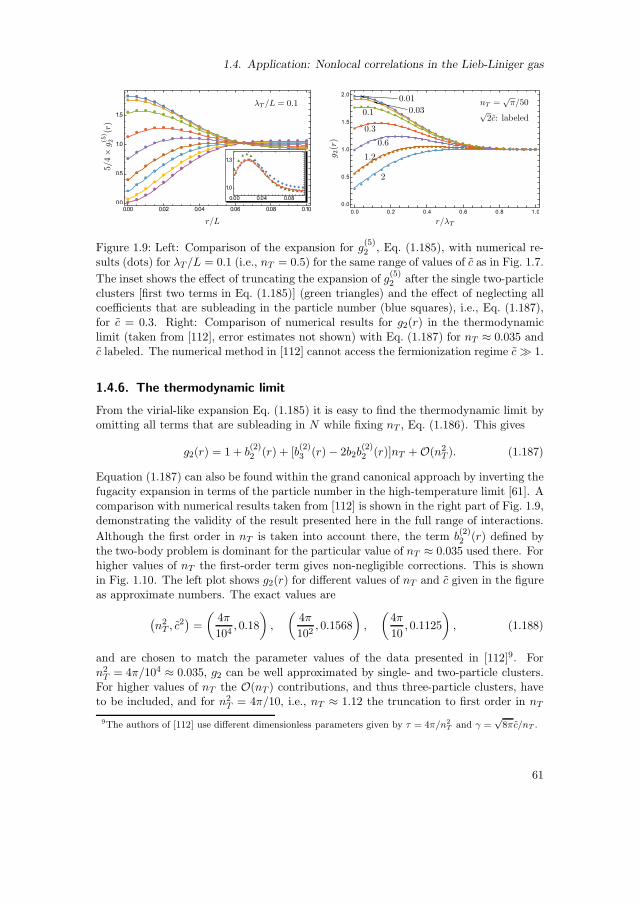
1.4. Application: Nonlocal correlations in the Lieb-Liniger gas
Figure 1.9: Left: Comparison of the expansion for g(5)2 , Eq. (1.185), with numerical re-
sults (dots) for λT /L = 0.1 (i.e., nT = 0.5) for the same range of values of c as in Fig. 1.7.
The inset shows the effect of truncating the expansion of g(5)2 after the single two-particle
clusters [first two terms in Eq. (1.185)] (green triangles) and the effect of neglecting allcoefficients that are subleading in the particle number (blue squares), i.e., Eq. (1.187),for c = 0.3. Right: Comparison of numerical results for g2(r) in the thermodynamiclimit (taken from [112], error estimates not shown) with Eq. (1.187) for nT ≈ 0.035 andc labeled. The numerical method in [112] cannot access the fermionization regime c≫ 1.
1.4.6. The thermodynamic limit
From the virial-like expansion Eq. (1.185) it is easy to find the thermodynamic limit byomitting all terms that are subleading in N while fixing nT , Eq. (1.186). This gives
g2(r) = 1 + b(2)2 (r) + [b
(2)3 (r) − 2b2b
(2)2 (r)]nT + O(n2T ). (1.187)
Equation (1.187) can also be found within the grand canonical approach by inverting thefugacity expansion in terms of the particle number in the high-temperature limit [61]. Acomparison with numerical results taken from [112] is shown in the right part of Fig. 1.9,demonstrating the validity of the result presented here in the full range of interactions.
Although the first order in nT is taken into account there, the term b(2)2 (r) defined by
the two-body problem is dominant for the particular value of nT ≈ 0.035 used there. Forhigher values of nT the first-order term gives non-negligible corrections. This is shownin Fig. 1.10. The left plot shows g2(r) for different values of nT and c given in the figureas approximate numbers. The exact values are
(n2T , c
2)
=
(4π
104, 0.18
)
,
(4π
102, 0.1568
)
,
(4π
10, 0.1125
)
, (1.188)
and are chosen to match the parameter values of the data presented in [112]9. Forn2T = 4π/104 ≈ 0.035, g2 can be well approximated by single- and two-particle clusters.For higher values of nT the O(nT ) contributions, and thus three-particle clusters, haveto be included, and for n2T = 4π/10, i.e., nT ≈ 1.12 the truncation to first order in nT
9The authors of [112] use different dimensionless parameters given by τ = 4π/n2T and γ =
√8πc/nT .
61

1. Quantum cluster expansions in short-time approximation
Figure 1.10: Left: Nonlocal pair correlation in the thermodynamic limit for differentinteraction strengths and different values of nT such that g2(0) ≈ 1. In the high-temperature or low-density regime nT ≪ 1 only two-particle clusters contribute. Forlower temperatures O(nT ) corrections cannot be neglected and larger clusters play arole. Right: Local correlations g2(0) with respect to the interaction parameter. Numer-ical data (dots) is taken from [118]. The approximation by two-particle clusters (graydashed) is sufficient for high temperatures (low densities). By including the next orderin the cluster expansion (solid line) we can see a major improvement in the regime oflower temperature.
is not sufficient anymore for a precise prediction but still gives reasonable qualitativeagreement with numerical calculations. The right part of Fig. 1.10 shows the localcorrelations g2(0) for a wide range of the interaction parameter. A major improvementin the agreement of numerical (taken from [118]) and semiclassical results can be seenwhen including the first-order correction in nT . Note that the local version g2(0) ofthe pair correlation can be calculated exactly by solving integral equations using theHellmann-Feynman theorem [118] (higher local correlation functions have been foundfrom viewing the LL model as a limiting case of the sinh-Gordon model [119]), but tothe best knowledge of the author, all published analytical results for g2(r) in the weaklydegenerate regime were derived in perturbation theory, i.e., they are only valid in thelimits of weakly or strongly interacting bosons. The result presented here, Eq. (1.187),represents the generalization of these results for arbitrary interaction strengths in themoderate- to high-temperature regime.
1.4.7. Summary and possible further applications
This section has demonstrated that the application of the short-time approximation tothe spatially dependent nonlocal pair correlation leads to essentially exact results fortemperatures well above the quantum degenerate regime while still giving good resultsclose to the latter. For the example of three particles it has been shown that the fullcluster expansion in short-time approximation remains valid up to λT ≈ L/2. In thissituation, the mean inter-particle distance L/N = 2λT /3 is already smaller than thethermal wavelength. It was then demonstrated that the universal scaling behavior in
62

1.4. Application: Nonlocal correlations in the Lieb-Liniger gas
the short-time approximation remains valid for higher particle numbers. This was doneby predicting the form of the nonlocal pair correlation function for a whole range oftemperatures using the numerically extracted values of the individual clusters at a fixedtemperature. Comparing the results obtained from this rescaling procedure to numericalcalculations shows very good agreement down to λT = 0.4L, corresponding to a thermalwavelength that is twice the mean particle separation. This underlines the validity ofthe short-time approximation also in this quantum regime with NλT /L ≥ 1.
For higher particle numbers approximations were presented that are valid well abovethe quantum degeneracy regime, i.e., NλT /L≪ 1, while still explicitly depending on theparticle number and thus explicitly accounting for its finiteness. Finally, by neglectingthe contributions that are subleading in the particle number, the exact results for thefirst two orders of the series expansion of g2(r) in the quantum degeneracy parameternT = NλT /L were calculated, and very good agreement with the numerical resultsobtained by other authors was shown. While this work awaits experimental confirmationin state-of-the-art experiments with 1D trapped quantum gases in the weak degeneracyregime, it is planned to extend the analysis to momentum correlations in the 1D Bosegas that have been measured recently [120].
Possible further applications could extend the results to the case of smooth externalpotentials, including the latter on the level of the short-time approximation. This allowsfor the transfer or the results from the quantum integrable Lieb-Liniger model to these
nonintegrable cases, where not only the analytical results for b(k)n for n = 1, 2, 3, but also
the numerically extracted results for n > 3 can be used.Another application in one-dimensional systems, apart from the straightforward mul-
tiple-species extensions that can range from dynamical impurities, to fermionic spin-1/2systems (i.e., the Gaudin-Yang model [108]) and mixtures of different species, couldbe the super-Tonks-Girardeau gas [121] that has been experimentally realized using aconfinement induced resonance [122], where the interaction changes from infinitely re-pulsive (Tonks-Girardeau) to infinitely attractive interaction (super-Tonks-Girardeau)by continuously tuning the scattering length of the three-dimensional interaction. Theidea is to use the results from the Lieb-Liniger gas also for the attractive case c < 0,however eliminating the bound states that are suppressed in the super-Tonks-Girardeaugas that gets dynamically stabilized, when approached from the Tonks-Girardeau gasregime, through the large kinetic energy in the latter. Thus, a large part of the complica-tions introduced in the calculation of the many-body propagator through the existenceof bound states is eliminated in this approach. As the smooth spectrum and nonlocalcorrelations of the Tonks-Girardeau gas mimic the respective properties of free spinlessfermions [123], one could use a fermionic model with an effective interaction to also applythe shifting method beyond the resonance.
63
1. Quantum cluster expansions in short-time approximation
1.5. Application: Short-range interaction in three dimensions
In this section, the methods of cluster expansions in short-time approximation will beapplied to three-dimensional (3D) systems. Although systems with lower dimensions cannowadays be prepared in experiments (as discussed in the last section), most systemsare three-dimensional in nature. It is probably for this reason that Beth and Uhlenbeckapplied the cluster expansion only to 3D systems when they first introduced its quan-tum formulation [66]. Their final result was the now-called Beth-Uhlenbeck formula forthe first virial coefficient that is determined by the two-particle problem and can beexpressed in terms of the scattering phases of the interaction potential. The strengthof this approach is that the scattering phases are rather simple to calculate and thusa wide variety of interaction potentials can be addressed. However, spatially resolvedquantities as well as information beyond the first virial coefficient are not included inthese results. As mentioned earlier, there have been attempts to generalize the Beth-Uhlenbeck formula either by introducing three-body scattering phases [90] or by Ursellexpansion [77], but explicit calculations beyond the perturbative regime have not beenrealized in this context. One reason for this could be the fact that the calculation ofthe single-particle propagators in three dimensions in the presence of a scattering po-tential cannot be given as a closed form expression except for very special potentialslike the Poschl-Teller potential [124]. Of course, approximations can be found usingthe general Lippmann-Schwinger equation [125], with the simplest one being the Bornapproximation, however leading to expressions that are perturbative in the potentialstrength. Here, the QCE(1) and other approximations introduced earlier in this thesis,that go beyond these approaches, will be used for short-range repulsive and attractiveinteractions by calculating the interaction contributions explicitly from the propagatorof the scattering problem in the low energy scattering limit.
1.5.1. The QCE(1) in three dimensions
When considering short-range interactions it is usually a reasonable assumption thatthe interaction potential is spherically symmetric, as is usually assumed in cold-atomquantum gases with Feshbach-tunable interactions [22, 29]. The goal is to calculate
the part of the (imaginary time) propagator of the relative motion δK(1)µ (r1, r0;β, α)
that enters the interaction contributions (1.120) and finally the reduction of the inter-and intra-cycle contributions in the QCE(1) to one-dimensional integrals. Thus, let usstart with the general treatment of two particles interacting via a spherically symmetricpotentials in an infinite volume. After separating off the motion of the center of mass,the Hamiltonian of the relative motion in position representation is simply given as
Hrel = − ~2
2µr + V (r) (1.189)
with r = |r| and the reduced mass µ and the spherically symmetric potential V (r). Theenergy eigenfunctions can then be decomposed into the spherical harmonics Ylm and the
64
1.5. Application: Short-range interaction in three dimensions
solutions ukl(r) of the radial equation as
ψklm(r) =ukl(r)
rYlm(θ, φ). (1.190)
The propagator for the relative motion can therefore be simplified using the additiontheorem for spherical harmonics [91],
K(1)µ (r1, r0;β, α) =
∞∑
l=0
l∑
m=−l
1
r1r0K
(1)µ,l (r1, r0;β, α)Ylm(θ1, φ1)Y ∗
lm(θ0, φ0)
=
∞∑
l=0
2l + 1
4πr1r0K
(1)µ,l (r1, r0;β, α)Pl(cos γ), (1.191)
where Pl is the lth Legendre polynomial and γ is the angle between r1 and r0. Theradial component of the propagator with angular momentum quantum number l is heredefined as
K(1)µ,l (r1, r0;β, α) =
∫ ∞
0dk e−β ~
2k2
2µ ukl(r1)u∗kl(r0) (1.192)
and scales like a one-dimensional propagator (c.f., Eq. (1.99) with Dtot = 1). Subtractingthe noninteracting part from the propagator will only affect the radial components, suchthat one can write it as
δK(1)µ (r1, r0;β, α) =
∞∑
l=0
2l + 1
4πr1r0δK
(1)µ,l (r1, r0;β, α)Pl(cos γ) (1.193)
or, using the general scaling (1.99) for δK, Eq. (1.126), one obtains
δk(1)(r1, r0; s) =
∞∑
l=0
2l + 1
4πr1r0δk
(1)l (r1, r0; s)Pl(cos γ) (1.194)
in terms of the dimensionless variables ri = ri/λT (µ). The dimensionless inter- andintra-cycle diagrams, Eqs. (1.128) and (1.132), are thus given as
ainter/intraν (s) =
∞∑
l=0
∫ ∞
0dx
∫ ∞
0dy δk
(1)l (x, y; s)f
inter/intraν,l (x, y) (1.195)
with
finter/intraν,l (x, y) = (2l + 1)
xy
4π
∫
dΩx dΩy1
ν3e−π(x∓y
ν )2
Pl(cos γ)
= (2l + 1)4πxy
ν3e−π
(
x2+y2
ν2
)
(∓i)ljl(
2πixy
ν2
)
. (1.196)
Here, jl is the lth spherical Bessel function (see [91] for the evaluation of the integral) andthe upper and lower sign stand for inter- and intra-cycle diagrams, respectively. Note
65
1. Quantum cluster expansions in short-time approximation
that iljl(it) is real for real values of t. The above result shows that the values of inter- andintra-cycle diagrams are the same for the even angular momentum quantum numbers lwhile they have the opposite sign for odd l. Combining this result with the multiplicities(1.130) and (1.133) of the diagrams, (1.196) shows that if the interacting particles areof the same species, their contributions vanish in the case of even(odd) values of l forfermions(bosons). This is a direct consequence of the parity of the spherical harmonicsin the case of two particles, where the exchange of the particles corresponds to theinversion of their relative coordinate. The calculation presented here thus shows thatthis property also holds in the QCE(1) as it should.
In the case of s-wave scattering, fν,0 simplifies drastically, yielding
f interν,0 (x, y) = f intraν,0 (x, y) =1
ν
[
e−π( x−yν )
2
− e−π(x+yν )
2]
. (1.197)
Remarkably, this has exactly the form of a single-particle propagator for a semi-infiniteline subject to a Dirichlet boundary condition at the origin [126].
1.5.2. Low-energy approximations and s-wave scattering
One of the assumptions that has been used in the preceding sections is the short-rangecharacter of the interaction. However, this has to be specified in terms of a differentlength scale of the system. In equilibrium systems as are considered here, one shouldcompare the range of the interaction to the thermal wavelength: If the latter is muchlarger than the extent of the interaction potential, the details of this potential cannotbe resolved by the average particle, i.e., only particles with a relative kinetic energy thatexceeds the average single-particle energy by far will be affected by the detailed formof the potential. In the partial wave analysis one would find that the scattering intowaves with l ≥ 1 is strongly suppressed, as the respective wave functions have to vanishat the center of the potential and are only slowly varying compared to the latter, thusbeing close to zero over the full range of the potential. Therefore, it is often sufficient totake only the s-wave scattering into account, especially in the low-temperature regimethat is addressed in cold atom experiments [22, 29]. One has to stress that the short-time approximation does not contradict this low-temperature assumption as long asthe thermal wavelength does not become comparable to the length scale given by thesystem size. If the latter is much larger than the range of the interaction, as is the casein almost all cold-atom experiments, there is a very big window where both short-timeapproximation and short-range interaction are perfectly consistent.
The low-energy scattering is then only determined by the s-wave scattering phase δsthat should then be consistently approximated by its low-energy (i.e., large wavelength)limit, where it is determined through the scattering length as as the only parameter. Tomodel this simple type of interaction that treats the potential as if it has no length, oneis tempted to do this with a point-like interaction by using an interaction potential ofthe form
Vint(r′, r) = “gδ(3)(r′ − r)” (1.198)
66
1.5. Application: Short-range interaction in three dimensions
with a 3D Dirac delta distribution, similar as in 1D. However, it turns out that modelingthis delta distribution, e.g., as a limiting case of a spherical step potential, its effect wouldvanish for any finite coupling strength g in the zero-range limit and it thus requiresregularization. There are different ways to achieve this, the most popular being theFermi or Fermi-Huang pseudo-potential [127–129] acting as (setting ~
2/2m = 1 for themoment)
VF(r)ψ(r) = 4πasδ(3)(r)
∂
∂r(rψ(r)) (1.199)
on the relative wave function. The effect of the derivative is to remove possible 1/rdivergences in the wave function that are forbidden in the noninteracting case, leadingto a nontrivial boundary condition
ψ(r) ∼ const ×(
1
r− 1
as
)
(1.200)
for r → 0 (The constant is nonzero only for the rotationally symmetric s-wave functions).One has to be careful, however, when interpreting the potential (1.199). Naively, onewould expect that a small attractive interaction leads to a small negative scatteringlength while the latter would be positive for repulsive interaction. However, the Fermipseudo-potential allows for a bound state solution for as > 0, with an energy that divergesfor as → 0+ (the plus sign indicating that as = 0 is approached from above), whilethis bound state is absent for negative scattering lengths. In more recent approaches,a momentum cutoff regularization [130–132] of the contact interaction is often used,however leading to the same results. This apparently unphysical behavior has led to someconfusion and inconsistency in the literature when it comes to the physical interpretationin terms of “attractive” and “repulsive” interaction.
There is, however, a perfectly meaningful interpretation of the above behavior. Inexperiments with tunable scattering length as, the latter is not a system parameter butrather a derived quantity. In cold atom experiments, the control of as is usually achievedusing Feshbach resonances [29], where the scattering length has the form
as =1
g − gres(1.201)
in the vicinity of the resonance value gres of the continuous parameter g that depends,e.g., on the magnetic field. Thus, the potential (1.199) is best interpreted as an effectivedescription around a resonance and would be better expressed in terms of a continuousparameter g, Eq. (1.201), such that the values as → 0± correspond to the regimesg → ∓∞ far to the left and far to the right of the resonance. The noninteracting casewould then correspond to the limit g → ∞, while it is natural to expect that a zeroenergy bound state appears at the resonance g = gres that has a negative energy forg < gres.
The soft-shell scattering potential
To clarify the above and to see how the resonance picture emerges naturally, it is in-structive to use a simple model potential with finite range rs to analyze the limit rs → 0.
67
1. Quantum cluster expansions in short-time approximation
This will then be used to derive the s-wave part of the propagator, i.e., Eq. (1.192) withl = 0. Let the relative potential of two particles be given as the soft-shell potential
V (r) =~2c
2µδ(1)(r − rs) (1.202)
with a finite shell radius rs and the potential strength c. It is equivalent to imposing the(mixed) boundary condition
limǫ→0
[d
drlog |ukl(r)|
]rs+ǫ
rs−ǫ
= c (1.203)
at the shell, where the left hand side means the difference of evaluating the bracketoutside and inside the shell and ukl(r) is the radial wave function defined in (1.190).Note that for the finite soft-shell potential 1.202 there is a clear definition of repulsiveand attractive interaction as c > 0 and c < 0, respectively.
It is straightforward to show that the scattering phases can be expressed as
tan δl =ck jl(krs)(
ck +
j′l(krs)
jl(krs)
)
nl(krs) − n′l(krs), (1.204)
with the spherical Bessel and Neumann functions jl and nl. Using the Wronskian [133]
n′l(x)jl(x) − nl(x)j′l(x) =1
x2(1.205)
leads to the simpler form
tan δl =j2l (krs)
jl(krs)nl(krs) − (crs · krs)−1. (1.206)
For large wavelengths compared to the potential range rs, i.e., krs ≪ 1 the knownexpansion for the Bessel and Neumann functions yield the low-energy scattering phases
tan δl = − 2l + 1
[(2l + 1)!!]2× (krs)
2l+1
1 + 2l+1crs
+ O((krs)2l+3). (1.207)
Thus, for every value of l there is a divergence at crs = −(2l+ 1) corresponding to a fastincrease of the respective scattering phase δl by π that coincides with the emergence ofa bound state, as shown in the following.
The equation for the bound states is obtained by matching the free solutions inside theshell to exponentially decaying solutions for r > rs (i.e., the spherical Hankel functionsh(1)(iκr) with imaginary argument) yielding the quantization
i j2l (iκrs)
nl(iκrs)jl(iκrs) − (crs · iκrs)−1= 1, (1.208)
68

1.5. Application: Short-range interaction in three dimensions
where the energy is given by E = −~2κ2
2µ if the solution exists. In the regime κrs ≪ 1the solutions can be found as
κrs =
[
4Γ(l + 5
2
)
Γ(l − 1
2
)
(1
crs− 1
2l + 1
)]12
, l > 0, (1.209)
κrs =1 + crscrs
, l = 0, (1.210)
where the condition for the existence is in all cases crs ≤ −(2l + 1), i.e., they appear(with zero energy) exactly at the divergences of tan δl, Eq. (1.207).
The above shows that there are many resonances already in this simple model. How-ever, as can be seen from Eq. (1.207), the s-wave scattering is dominant away from theresonances. One can directly read off the scattering length as
as = −[
limk→0
k cot δ0
]−1
=crs
crs + 1rs. (1.211)
The zero-range Fermi pseudo-potential now turns out to have exactly the same scatteringand bound states as the shell potential in the limit rs → 0, keeping the parameterc = c+ 1/rs fixed to stay in the vicinity of the s-wave resonance. The reason for this isthe different position of the resonances of scattering phases for l > 0 thus yielding thetrivial limit δl → 0 in the zero-range limit as for the Fermi pseudo-potential. However,in this limit, the parameter regime of repulsive interactions c > 0 is pushed to c = ∞and can therefore not be accessed anymore.
To conclude the above, the pseudo-potential (1.199) and equivalent regularized zero-range potentials should only be used in the vicinity of a s-wave resonance. There, itdoes not make sense to interpret a positive scattering length as > 0 as an indicator forrepulsive interaction. As the resonance is accompanied by the formation of a bound state,one should rather understand the potential as attractive for all values of the scatteringlength. In other words, a repulsive zero-range potential has no effect (if internal degreesof freedom of the particles are left unaccounted for).
However, we are now in the position to say something also for the more general case,as we do not have to take the zero-range limit as long as we stay in the low-energy regimekrs ≪ 1 to justify the description of interactions only in terms of the scattering length(1.211) (and the bound state for crs < −1).
The low-temperature imaginary-time propagator for a soft-shell potential
As was discussed earlier, we can make use of the short-time approximation of propagatorsevaluated in imaginary time while still being in a regime where the thermal wavelengthis much larger than the range of interactions, therefore having to include only the low-energy effects of the interaction. One can thus calculate an approximation of the s-wavepart of the imaginary-time propagator (1.192) for the soft-shell potential (1.202) byreplacing the radial wave functions uk0 by their low-energy approximations using
tan δ0 = kas (1.212)
69

1. Quantum cluster expansions in short-time approximation
for all k and noting that error gets suppressed at low temperatures, when λT ≫ rs.Specifically, for krs & 1 we have
βEk,rel =~2k2β
2µ=λ2T (µ)k2
4π&λ2T (µ)
4πr2s≫ 1, (1.213)
such that the respective contributions in the imaginary-time propagator are stronglysuppressed due to their weighting with exp(−βEk,rel).
To calculate the s-wave part of the propagator, Eq. (1.192) with l = 0, the relativemotion is enclosed in a finite, but large volume, e.g., a large sphere with radius R ≫rs, that quantizes the values of k and fixes the normalization and is sent to R → ∞afterwards. Here, only the results are presented, and the reader is referred to AppendixC for the detailed derivations. Also, it is assumed that the initial and final coordinateslie outside the potential shell. In this case, the correction to the s-wave part of thepropagator can be written as
δK(1)µ,0(r1, r0;β, α) =
1
λT (µ)δk
(1)0 (r1 + r0, 0; s), (1.214)
δk(1)0 (z, 0; s) = 2e−πz2
[
1 ± πseπ(z+s)2 erfc(∓√
π(z + s))]
(1.215)
with the complementary error function erfc and the scaled variables
z = r1 + r0 =r1 + r0λT (µ)
, s = −λT (µ)
2πas. (1.216)
The upper and lower sign in (1.215) correspond to the repulsive (c > 0) and attractive(c < 0) case, respectively. Note that the variable s is of the form
√αβ rather than αβ
used before, with α being an energy-like parameter. The reason for this choice is thefact that the sign of s then encodes the sign of the scattering length as.
The result for the attractive case exactly reproduces the interaction part of the (real-time) propagators found either using the (unique) self-adjoint extension of the Hamilto-nian for a point interaction [134,135] as well as for the Fermi pseudo-potential [84] andthe momentum-cutoff regularization of a delta-potential [132], showing the equivalenceof the respective approaches.
It is instructive to see how the repulsive result differs from the attractive one. Thiscan be seen by rewriting the complementary error function in (1.215) for the repulsivecase as
− erfc(−√
π(z − s))
= erfc(√π(z − s)
)− 2, (1.217)
such that the result differs from the attractive case with s > 0 by
− 4πse−πz2+π(z−s)2 = −Ψb(z, s). (1.218)
It is easily verified that this exactly cancels the bound state contribution present in theattractive regime beyond the resonance, such that the low-temperature imaginary-timepropagator for the repulsive soft-shell potential can be obtained from the known results
70

1.5. Application: Short-range interaction in three dimensions
by dropping the bound state contribution, as long as the two coordinates lie outside thepotential sphere.
If one or more of the coordinates are within the sphere, there are additional contri-butions (see Appendix C) that vanish in the limit of a point potential. One can easilyargue that, within QCE(1), the condition rs ≪ λT implies that the latter contributionsare negligible as the propagator is smeared with normal distributions according to Eqs.(1.197) and (1.195), with a width ν large compared to the potential range rs/λT ≪ 1
for any cluster size. Also in the special case ν = 0, that yields the trace of δk(1)0 , the
contribution from within the potential is negligible.This means that we can use the s-wave interaction correction (1.215) for the propagator
together with the scattering length as in terms of the potential strength c and the finiterange rs, Eq. (1.211). By neglecting the contributions from l > 0 in Eq. (1.194) thisyields the approximate interaction part of the propagator
δk(1)(r1, r0; s) ≈ 1
4πr1r0δk
(1)0 (r1, r0; s) (1.219)
that will be used in the following.One should, however, make a few comments when it comes to repulsive interactions
in the simple model used here. The scattering length of the shell potential used in thederivation is bounded by rs for the case c > 0, with rs being the scattering length ofthe hard-sphere potential obtained for c → ∞. Therefore, if one wants to stick withthe simple model, one has to keep the potential range rs finite to obtain a nontrivialresult. The low-temperature limit sketched above then corresponds to the perturbativeregime |s−1| ≪ 1 or as ≪ λT according to Eqs. (1.213) and (1.216), such that the s-wavescattering approach would be rather trivial in this regime, only yielding known results(see, e.g., [68]). But we have seen that the analytic form of the propagator for c > 0, whenexpressed through the scattering length as or equivalently s is exactly the same as for aresonance, except for the missing bound state. Therefore, one could equally well forgetabout the (hidden) dependence on the parameter c and simply use the propagator forthe “repulsive” interaction in situations, where a resonance is approached from below(as > 0) while only taking into account the scattering states that are adiabaticallyconnected to the scattering states of a weakly repulsive interaction.
This approach is actually closer to experimental setups than the use of the modelpotential introduced above: A real gas of cold atoms usually hosts molecular boundstates that actually render the gas metastable, leading to inelastic scattering and parti-cle losses in experiments that are, however, strongly suppressed due to weak coupling ofthe respective molecular and atomic states. In cold atom gases, the internal degrees offreedom of the atoms lead to many different scattering channels, with most of them beingclosed at very low temperatures, but with closed-channel bound states that can lie veryclose to the continuum threshold energy of an open channel. If such a closed channelbound state can be energetically tuned by external parameters to approach the contin-uum, even a weak coupling between this state and the open-channel scattering states caninduce a Feshbach resonance [29]. The situation of approaching such a resonance from“below” then just means that the molecular bound state in the closed channel is initially
71

1. Quantum cluster expansions in short-time approximation
Figure 1.11: Sketch of the parametrization of the interactions used in the following. Inthe attractive case, the scaled interaction s, Eq. (1.216), describes the regime around aresonance with a bound state being created at s = 0 and a bound state energy Eb ∝ −s2(sketched in dashed blue). The limit s→ ∞ corresponds to the noninteracting limit. Inthe repulsive case, s is only used as a parametrization of the scattering length, that canhave any dependence on a tunable parameter, and diverges when (another) resonanceat s = 0 is approached adiabatically from the left. Although a bound state has toexist also at this resonance (sketched in dashed red), it is not taken into account in thecalculations, assuming that it is adiabatically decoupled from the scattering states andinelastic scattering subdominant.
below the continuum threshold. The finite “background scattering length” (given by rsin the soft-shell potential model above) plays a role in the characterization of Feshbachresonances, but a universal description is applicable in the region of diverging scatteringlength [29], where the resonance has exactly the shape modeled by the shell potential atits s-wave resonance, with a (hybrid) bound state that has exactly the same propertiesbut is adiabatically connected to a closed-channel molecular state. Even though a Fes-hbach resonance is subject to enhanced particle losses and molecule formation at thisuniversal regime [29], one should expect that the scattering states dominate the physicswhen the resonance is approached from below, as the molecular state is dynamically in-accessible well below the resonance. In contrast, the bound state should not be ignored,when tuning across the resonance from above, as the molecular state then connects tothe continuum10.
The above adiabatic exclusion of the bound state is assumed in the following, when“repulsive” interaction is considered, i.e., it is assumed that one can adiabatically tunethe system from the noninteracting case to the vicinity of a resonance, where the scat-tering states are obtained adiabatically from the noninteracting states and the boundstate can be ignored. This situation is exactly described by the soft-shell propagator forthe “repulsive” interaction. Note that the parameters c and rs of the soft-shell potentialthen lose their meaning for as > rs and are therefore not further used. Figure 1.11summarizes the notion of “attractive” and “repulsive” interaction that is assumed here,and illustrates the parametrization through the parameter s ∝ a−1
s , that changes from∞ to −∞ when switching from attractive to repulsive.
10This can actually be used for adiabatic atom-molecule conversion in ultracold atomic gases [29]
72

1.5. Application: Short-range interaction in three dimensions
1.5.3. The short-range interacting Bose gas
In this section, some of the methods of the previous sections are applied to a Bose gaswith dominant s-wave scattering.
Nonlocal correlations
As a “low-hanging fruit”, one can consider the nonlocal correlation function in thethermodynamic limit to leading order in its virial expansion (1.187). The universaldensity-independent part that dominates the high-temperature regime is given by
g2(r) = 1 + b(2)2 (r) (1.220)
also in the case of three dimensions, where the first term corresponds to the “classical”
correlation being constant. The function b(2)2 (r) only depends on the distance r of the
particles and is easily calculated from (1.215) as
b(2)2 (r) = e−4πr2 +
1
πr2e−4πr2
[
1 ± πse4π(r+s/2)2 erfc(
∓√
4π(r + s/2))]
. (1.221)
Here, as before, the upper sign stands for the repulsive case (i.e., it excludes the boundstate) while the lower sign is valid for the attractive case, also across the resonance. Inthe noninteracting case (s→ ±∞ for the attractive, respective repulsive case), only thefirst term remains, corresponding to the cyclic permutation of two particles. It describesthermal bunching of bosons, increasing the local correlations at r = 0 by a factor oftwo. When interactions are switched on, the correlations diverge at the origin as anartifact of the point-like approximation of the potential. One thus has to take intoaccount a finite radius rs of the interaction potential that is used as a lower cutoff inthe distance or one can use the expression for the model shell-potential propagator forr < rs given in Appendix C to obtain a regular expression also for this regime. However,when considering the radial distribution
g(rad)2 (r) =
∫
dΩ r2g2(r) = 4πr2g2(rer), (1.222)
that is proportional to the probability of finding two particles in a distance r, the diver-gence is removed and yields finite correlations at the origin, that can only be positive,irrespective of the type of interactions, as the pair correlation has to be positive every-where.
For completeness, let us also consider the scaling of the pair correlation function inspecific limits. For an infinitesimal scattering length, one obtains
g2(r) = 1 + e−4πr2[
1 − 4asr
]
+ O(a2s ), (1.223)
valid for both attractive and repulsive regime, while first expanding g2 with respect tor reveals the short-range scaling
g2(r) ≈ 2(
1 − asr
)2(1.224)
73
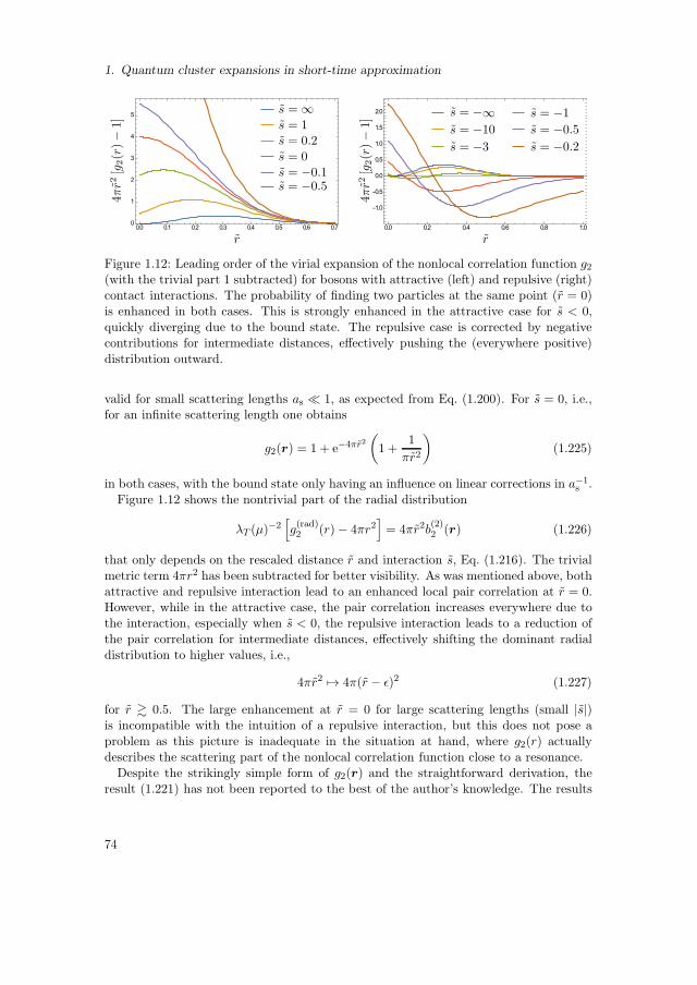
1. Quantum cluster expansions in short-time approximation
Figure 1.12: Leading order of the virial expansion of the nonlocal correlation function g2(with the trivial part 1 subtracted) for bosons with attractive (left) and repulsive (right)contact interactions. The probability of finding two particles at the same point (r = 0)is enhanced in both cases. This is strongly enhanced in the attractive case for s < 0,quickly diverging due to the bound state. The repulsive case is corrected by negativecontributions for intermediate distances, effectively pushing the (everywhere positive)distribution outward.
valid for small scattering lengths as ≪ 1, as expected from Eq. (1.200). For s = 0, i.e.,for an infinite scattering length one obtains
g2(r) = 1 + e−4πr2(
1 +1
πr2
)
(1.225)
in both cases, with the bound state only having an influence on linear corrections in a−1s .
Figure 1.12 shows the nontrivial part of the radial distribution
λT (µ)−2[
g(rad)2 (r) − 4πr2
]
= 4πr2b(2)2 (r) (1.226)
that only depends on the rescaled distance r and interaction s, Eq. (1.216). The trivialmetric term 4πr2 has been subtracted for better visibility. As was mentioned above, bothattractive and repulsive interaction lead to an enhanced local pair correlation at r = 0.However, while in the attractive case, the pair correlation increases everywhere due tothe interaction, especially when s < 0, the repulsive interaction leads to a reduction ofthe pair correlation for intermediate distances, effectively shifting the dominant radialdistribution to higher values, i.e.,
4πr2 7→ 4π(r − ǫ)2 (1.227)
for r & 0.5. The large enhancement at r = 0 for large scattering lengths (small |s|)is incompatible with the intuition of a repulsive interaction, but this does not pose aproblem as this picture is inadequate in the situation at hand, where g2(r) actuallydescribes the scattering part of the nonlocal correlation function close to a resonance.
Despite the strikingly simple form of g2(r) and the straightforward derivation, theresult (1.221) has not been reported to the best of the author’s knowledge. The results
74

1.5. Application: Short-range interaction in three dimensions
for the s-wave part of a gas of hard spheres can be calculated analytically without usingthe low-energy approximation [136, 137]. The results are equivalent for a small sphereradius compared to the thermal wavelength, i.e., in the regime where s-wave scatteringis dominant.
The density of states
We are now in the position to actually calculate all the clusters that appear within theQCE(1) by using the general formulas (1.195) and (1.197) for the inter- and intra-cyclediagrams with the s-wave interaction correction (1.215). The calculations can be short-ened a bit by using the fact that the interaction-independent part of (1.215) is exactlycanceled in the noninteracting limit (given by s → ∞ and s → −∞ in the attractiveand repulsive regime, respectively) and thus is included in the coupling-dependent term.The calculation is straightforward, yielding for the repulsive case
ainter/intraν (s) = − 1
π
ν
1 + ν2+
ν2√π√
1 + ν2
√s+
ν√π
√s es erfc
(√s)
− 1 + 2ν2s
2
[
G(ν)0
((1 + ν2)s
)+ e(1+ν2)s erfc
(√
(1 + ν2)s)]
. (1.228)
Here, to make the notation consistent, the coupling s is of the form
s = πs2 ≡ αβ > 0, α =~2
µa2s, (1.229)
and the function G(ν)0 is defined as
G(ν)0 (s) =
2√π
es∫ ∞
0dz e−(z+
√s)
2
erf(νz), (1.230)
where the index 0 is only introduced for consistency with later definitions. For ν = 0,i.e., in the case of a two-particle cluster, the expressions simplify to
ainter/intra0 (s) = −1
2es erfc(
√s). (1.231)
In the attractive case, the scattering length can be either positive or negative. As thecoupling s cannot have negative values, one has to introduce an additional parameter
η = − sgn(as) = sgn(s) (1.232)
to distinguish the two cases. Here, η = 1 represents the regime from the noninteractingcase (s → ∞) to the resonance (s = 0) while η = −1 covers the regime beyond theresonance, where the s-wave bound state is present. The result for the attractive case isthen given by
ainter/intraν (s) = − 1
π
ν
1 + ν2− η
ν2√π√
1 + ν2
√s+ η
ν√π
√s es erfc
(η√s)
− 1 + 2ν2s
2
[
G(η,ν)0
((1 + ν2)s
)− e(1+ν2)s erfc
(
η√
(1 + ν2)s)]
. (1.233)
75
1. Quantum cluster expansions in short-time approximation
The function G(η,ν)0 is defined as
G(η,ν)0 (s) =
2√π
es∫ ∞
0dz e−(ηz+
√s)
2
erf(νz). (1.234)
Again, the result simplifies drastically for ν = 0, yielding
ainter/intra0 (s) =
1
2es erfc(η
√s) = η
1
2es erfc(
√s) + Θ(−η)es. (1.235)
To obtain the density of states, one has to use these expressions to calculate first thepartition function and then its inverse Laplace transform. This leads to the functions
g(N,d)l,+ (ǫ), Eq. (1.113), that alter the coefficients in the cluster expansion of N (N,d)(E).
By using the expansion (1.134) of ∆1z(N,d)1 into clusters one directly obtains
g(N,d)l,+ (ǫ) = 8ǫ−
ld2
N−l+1∑
n=2
n−d2 z
(N−n,d)l−1,+
n−1∑
n1=1
L−1s
[
s−ld2−1aν(n1,n−n2)(s)
]
(ǫ), (1.236)
where the labels for inter- and intra-cycle diagrams have been omitted, as the respectivediagram values are the same. The inverse Laplace transforms in Eq. (1.236) can beexplicitly performed for arbitrary l, but the calculations are rather technical and havetherefore been moved to Appendix D.4, where also more general functions can be foundthat appear in the QCE(2).
The full QCE(1) can be readily applied to different particle numbers and variousinteractions for the cases of a homogeneous Bose gas (d = 3) and for harmonic trapping(d = 6). Figure 1.13 shows the repulsive case in a comparison of the QCE(1) results withthe result from the first-order shifting method described in section 1.3.5 using the scaledvariables αsc, Esc, Eq. (1.142). As the QCE(1) result for the counting function N (N,d)
takes negative values for small energies, the plots show the absolute values of N (N,d) inthe respective approximations. The noninteracting limit αsc → ∞ is presented as a solidblue line in all plots. The left plot shows the case of three particles with very stronginteractions, with αsc = 0 corresponding to an infinite scattering length. As can be seen,both methods tend to the same results for large energies, but differ quite strongly at lowenergies, with the QCE(1) result even becoming negative in a whole range of energiesthat is well covered by the shifting method. The same behavior is seen for intermediatecouplings αsc = 10 in the right plot, where the counting function for N = 8 is shownfor two different effective dimensions, with d = 3 corresponding to the homogeneouscase and d = 6 describing harmonic confinement in short-time approximation. TheQCE(1) result cannot be trusted up to very large excitations in both case, while theshifted counting function yields converged results for all relevant energies. In the caseof N = 8 and d = 6, the energy of the result from the shifting method has been cutoff at approximately Esc = 0.5, where the self-consistent solutions for the shifts start towildly oscillate. This should, however, be attributed to numerical errors, also leading tonumerically induced noise in the QCE(1) result at small energies (not shown).
When the particle number is increased, one can expect the shifts to become universalfunctions that only depend on the scaled energy Esc and interaction αsc, as well as the
76
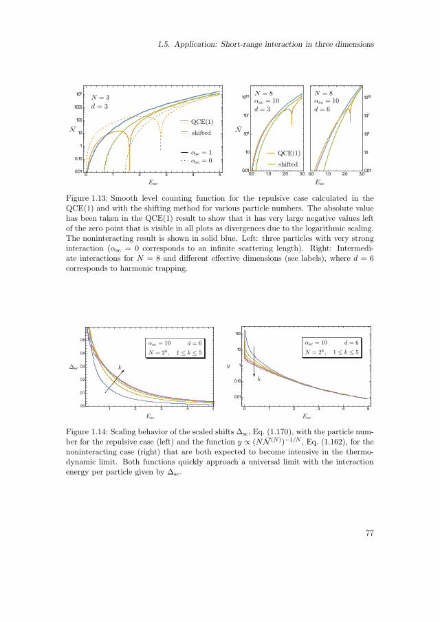
1.5. Application: Short-range interaction in three dimensions
Figure 1.13: Smooth level counting function for the repulsive case calculated in theQCE(1) and with the shifting method for various particle numbers. The absolute valuehas been taken in the QCE(1) result to show that it has very large negative values leftof the zero point that is visible in all plots as divergences due to the logarithmic scaling.The noninteracting result is shown in solid blue. Left: three particles with very stronginteraction (αsc = 0 corresponds to an infinite scattering length). Right: Intermedi-ate interactions for N = 8 and different effective dimensions (see labels), where d = 6corresponds to harmonic trapping.
Figure 1.14: Scaling behavior of the scaled shifts ∆sc, Eq. (1.170), with the particle num-ber for the repulsive case (left) and the function y ∝ (NN (N))−1/N , Eq. (1.162), for thenoninteracting case (right) that are both expected to become intensive in the thermo-dynamic limit. Both functions quickly approach a universal limit with the interactionenergy per particle given by ∆sc.
77

1. Quantum cluster expansions in short-time approximation
effective dimension d, Eq. (1.104). This has been demonstrated for the Lieb-Liniger gasand harmonically trapped bosons in 1D in [60] and also holds true for the case at hand,as the difference in the theory is only due to the different physical dimensions. Theasymptotic calculations are straightforward, but unfortunately have not been performedyet due to time constraints. To assess the applicability of the expected asymptotic uni-versal functions, Fig. 1.14 shows the tendencies of the scaled shifts ∆sc, Eq. (1.170), andthe noninteracting function y(Esc,∞), Eq. (1.162), towards their limiting functions. Thelatter is used in the shifting method and should become an intensive quantity accordingto the asymptotic ensemble equivalence discussed in section 1.3.4, being verified here fornoninteracting bosons with harmonic trapping. The calculated shifts in the left figureshow numerical noise for N = 16 and N = 32 that stems from the Gamma functions andfactorials that appear in the coefficients of the counting function, leading to large can-cellations. This could be cured by increasing the accuracy, but the preferred approachshould be the use of the asymptotic results that naturally include also the corrections ofthe function y for small energies through the amplitudes in Eq. (1.153) and should yieldcomparable results with less computational efforts.
Unfortunately, the author has not yet been able to compare the above results to full-fledged numerical calculations and/or experiments. The shifting method, in contrast tothe QCE(1) is able to predict a mean energy shift of the noninteracting levels in a waythat goes far beyond the perturbative regime, thus requiring the respective data for awide range of energies and interactions to benchmark. This could be addressed usingMonte-Carlo path integral approaches in the temperature regime similar to [17], but hasnot been done so far, and the results above have to be considered as work in progress.Also, although the results for the attractive interaction are also available here, theyhave not been used for bosons so far. However, the next subsection uses the attractiveinteraction for a small system of spin-1/2 fermions in a certain approximation.
1.5.4. The unitary Fermi gas—a few-particle perspective
A gas of spin-1/2 fermions with attractive short-range interactions in three dimensionsis known to have very interesting properties. In the noninteracting case, the gas can bedescribed by a Fermi sea with excitations above it. However, already for weak attractiveinteractions, this Fermi sea becomes unstable and the BCS theory of superconductivitypredicts a pairing of particles with opposite spin and momentum to Cooper pairs [12],that are, however, not localized in space. For stronger attractive forces, bound states ofthe relative potentials allow for the formation of molecules that get localized in space,with the most favorable configuration being the pairing of two fermions with oppositespin, i.e., singlet states, as the interaction between two fermions with the same spin issuppressed due to the Pauli principle that forces the wave function to vanish at shortdistances. If the pairing forces are strong enough, the molecules can be described ascomposite bosons with a weak residual interaction, leading to Bose-Einstein condensa-tion at low temperatures. Although the two limits seem to behave quite different atfirst glance, suggesting a transition between different types of physics, they are actuallyadiabatically connected by a crossover known as the BCS-BEC crossover [131,138]. De-
78
1.5. Application: Short-range interaction in three dimensions
spite both limits being well understood, the crossover regime hosts complicated physicsand does not allow for a mean-field description due to strong many-body correlations.One can define a special point in the crossover that is characterized by the divergenceof the two-body scattering length when a zero-energy molecular state is formed. This isreferred to as the unitary point or unitary limit, as the s-wave scattering cross section
σ0 =4π
k2sin2 δ0 →
4π
k2(1.237)
assumes its maximally allowed value, only restricted through the unitarity of the scat-tering matrix. Note that the fermions can only interact through s-wave scattering if theyhave different spin due to the Pauli principle. In the unitary limit (and at low enoughtemperatures), the physics should become independent of the length scales of the inter-action potential, such that it can be modeled by a zero-range potential. For the latter,being an effective description in terms of boundary conditions of the wave function, aseries of exact relations have been derived, known as Tan’s relations [139–141] that in-troduce a quantity known as Tan’s contact that describes the short-range correlations,but also appears in the spectral properties and can be calculated from an analogue ofthe Hellmann-Feynman theorem named as “adiabatic sweep theorem” by it’s inventor,
∂E
∂(−1/as)=
~2V C
4πm, C = lim
|k|→∞k4nk,σ. (1.238)
Here, C is Tan’s contact and nk,σ is the momentum distribution of the particles withspin σ. The energy E is thereby associated to any stationary state. The contact, as ameasurable quantity [142], has attracted a lot of attention especially in the descriptionof the crossover regime (see, e.g., [88, 143, 144] and references therein) as a nontrivialquantity in a highly correlated system.
It is, however, worth noting that the sweep relation for the contact shows that it isdirectly connected to the energy shift due to the finite inverse scattering lengths as theyappear in the applications considered here. To be specific, the shifting method used forbosons directly outputs the quantity that defines the contact for a generic eigenstate.It would thus be desirable to calculate the contact using the methods introduced here.However, this has not been done to date, but a first attempt that used the large Nasymptotic expressions (i.e., the stretch exponential form of the density of states) didnot yield satisfactory results when approaching the unitary limit, where some results areavailable in the literature. Instead, this section concentrates on the calculation of thecluster expansion for four fermions as a first testing ground for the applicability of theshifting and to reproduce the physics of the whole range of interactions (of course notobserving superconductivity in this few-particle system).
The QCE(1) is obviously not capable of producing two molecular states, as it containsonly a single two-particle bound state. Thus, to cover also the limit of two (composite)bosons interacting via a residual interaction one has to include also the QCE(2) dia-grams. However, as only the interaction contributions of second order, associated withthe second Ursell operator, is known, the higher interaction contributions are left out.They are expected to be subdominant, as they have to involve at least two identical
79
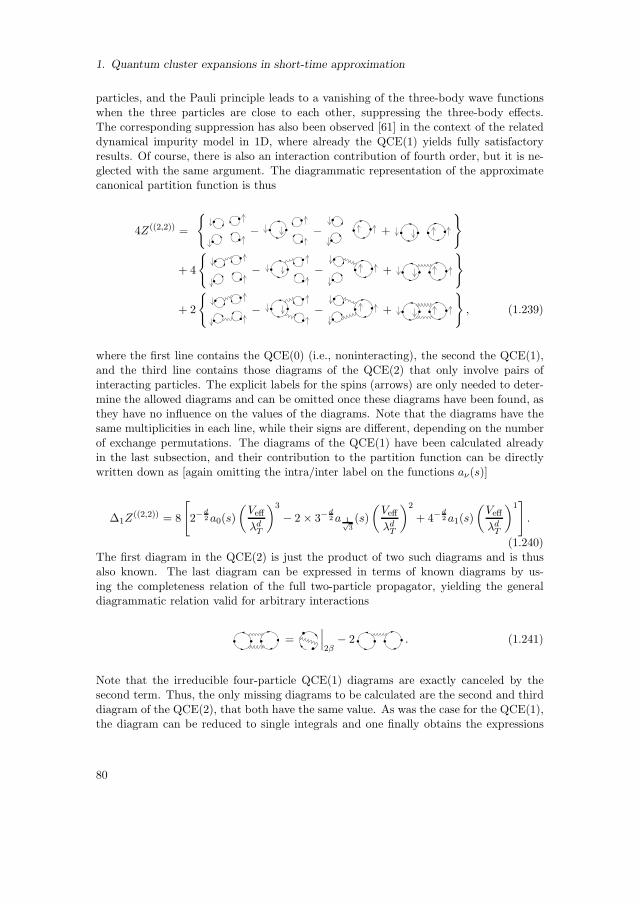
1. Quantum cluster expansions in short-time approximation
particles, and the Pauli principle leads to a vanishing of the three-body wave functionswhen the three particles are close to each other, suppressing the three-body effects.The corresponding suppression has also been observed [61] in the context of the relateddynamical impurity model in 1D, where already the QCE(1) yields fully satisfactoryresults. Of course, there is also an interaction contribution of fourth order, but it is ne-glected with the same argument. The diagrammatic representation of the approximatecanonical partition function is thus
4Z((2,2)) =
− − +
+ 4
− − +
+ 2
− − +
, (1.239)
where the first line contains the QCE(0) (i.e., noninteracting), the second the QCE(1),and the third line contains those diagrams of the QCE(2) that only involve pairs ofinteracting particles. The explicit labels for the spins (arrows) are only needed to deter-mine the allowed diagrams and can be omitted once these diagrams have been found, asthey have no influence on the values of the diagrams. Note that the diagrams have thesame multiplicities in each line, while their signs are different, depending on the numberof exchange permutations. The diagrams of the QCE(1) have been calculated alreadyin the last subsection, and their contribution to the partition function can be directlywritten down as [again omitting the intra/inter label on the functions aν(s)]
∆1Z((2,2)) = 8
[
2−d2 a0(s)
(Veff
λdT
)3
− 2 × 3−d2 a 1√
3(s)
(Veff
λdT
)2
+ 4−d2 a1(s)
(Veff
λdT
)1]
.
(1.240)The first diagram in the QCE(2) is just the product of two such diagrams and is thusalso known. The last diagram can be expressed in terms of known diagrams by us-ing the completeness relation of the full two-particle propagator, yielding the generaldiagrammatic relation valid for arbitrary interactions
=∣∣∣2β
− 2 . (1.241)
Note that the irreducible four-particle QCE(1) diagrams are exactly canceled by thesecond term. Thus, the only missing diagrams to be calculated are the second and thirddiagram of the QCE(2), that both have the same value. As was the case for the QCE(1),the diagram can be reduced to single integrals and one finally obtains the expressions
80

1.5. Application: Short-range interaction in three dimensions
for all the above QCE(2) diagrams as
= 64 × 2−da20(s)
(Veff
λdT
)2
, (1.242)
= 8Veff
λdT4−
d2 [a0(2s) − 2a1(s)], (1.243)
= −32Veff
λdT4−
d2
4 G(η,
√2)
0 (4s) − 4 H(η,1,
√2)
0 (4s)
, (1.244)
with the function G(η,ν)0 defined in Eq. (1.234) of the last subsection and the function
H(η,λ,µ)0 (s) =
2√π
es∫ ∞
0dz e−(ηz+
√s)
2
erf(λz) erf(µz). (1.245)
By reordering according to powers of Veff/λdT one obtains the coefficients ∆z
(N,d)l in
Eq. (1.108),
∆z(4,d)3 (s) = 8 × 2−
d2 a0(s), (1.246)
∆z(4,d)2 (s) = 16
[
21−da20(s) − 3−d2 a 1√
3(s)
]
, (1.247)
∆z(4,d)1 (s) = 4 × 4−
d2
a0(2s) − 8[
4 G(η,
√2)
0 (4s) − 4 H(η,1,
√2)
0 (4s)]
, (1.248)
that then define the coefficient functions g(4,d)l (ǫ) in the level counting function (1.112)
according to Eq. (1.113). The required inverse Laplace transforms can be found inAppendix D.4. Although the results above are valid also for homogeneous external po-tentials, the results for the inverse Laplace transform of s−d/2 H0 is only given as a closedform expression for odd effective dimension d. Although the case of even dimensions canbe easily implemented using a semi-analytical approach with one single numerical con-volution integral being required, only the case without external potentials is discussedhere.
Figure 1.15 shows a comparison of the QCE(1) predictions and the prediction fromincluding the diagrams from the QCE(2). There, the natural dimensionless couplingparameter
ρeffα =1
π
(
V1d
as
)2
(1.249)
is used, that emerges when the energy is expressed in terms of the energy unit ρ−1eff ,
Eq. (1.114). As can be seen, both approximations yield similar results for the regimewith negative scattering length, i.e., η = 1, where no bound states are available. This isdemonstrated in green for a rather strong coupling ρeffα = 1. Unfortunately, the QCE(2)result suffers from oscillations for small energies, yielding unphysical negative values forN there. In the presence of the bound states, i.e., for η = −1, the two results startto differ also for large excitations (orange) and when approaching the regime of large
81
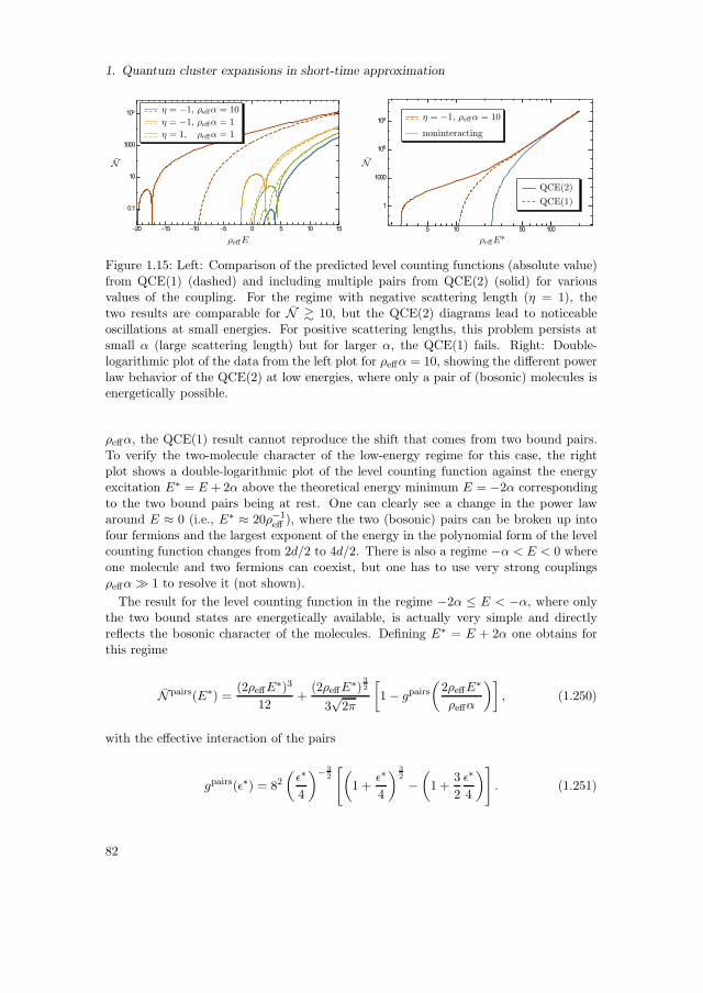
1. Quantum cluster expansions in short-time approximation
∗
Figure 1.15: Left: Comparison of the predicted level counting functions (absolute value)from QCE(1) (dashed) and including multiple pairs from QCE(2) (solid) for variousvalues of the coupling. For the regime with negative scattering length (η = 1), thetwo results are comparable for N & 10, but the QCE(2) diagrams lead to noticeableoscillations at small energies. For positive scattering lengths, this problem persists atsmall α (large scattering length) but for larger α, the QCE(1) fails. Right: Double-logarithmic plot of the data from the left plot for ρeffα = 10, showing the different powerlaw behavior of the QCE(2) at low energies, where only a pair of (bosonic) molecules isenergetically possible.
ρeffα, the QCE(1) result cannot reproduce the shift that comes from two bound pairs.To verify the two-molecule character of the low-energy regime for this case, the rightplot shows a double-logarithmic plot of the level counting function against the energyexcitation E∗ = E + 2α above the theoretical energy minimum E = −2α correspondingto the two bound pairs being at rest. One can clearly see a change in the power lawaround E ≈ 0 (i.e., E∗ ≈ 20ρ−1
eff ), where the two (bosonic) pairs can be broken up intofour fermions and the largest exponent of the energy in the polynomial form of the levelcounting function changes from 2d/2 to 4d/2. There is also a regime −α < E < 0 whereone molecule and two fermions can coexist, but one has to use very strong couplingsρeffα≫ 1 to resolve it (not shown).
The result for the level counting function in the regime −2α ≤ E < −α, where onlythe two bound states are energetically available, is actually very simple and directlyreflects the bosonic character of the molecules. Defining E∗ = E + 2α one obtains forthis regime
N pairs(E∗) =(2ρeffE
∗)3
12+
(2ρeffE∗)
32
3√
2π
[
1 − gpairs(
2ρeffE∗
ρeffα
)]
, (1.250)
with the effective interaction of the pairs
gpairs(ǫ∗) = 82(ǫ∗
4
)− 32
[(
1 +ǫ∗
4
) 32
−(
1 +3
2
ǫ∗
4
)]
. (1.251)
82

1.5. Application: Short-range interaction in three dimensions
By comparing this to the counting function for two bosons with contact interaction,
N (2)(E) =(ρeffE)3
12+
(ρeffE)32
3√
2π
[
1 − g
(E
α
)]
, (1.252)
g(ǫ) = 8ǫ−32
[
(1 + ǫ)32 −
(
1 +3
2ǫ
)]
, (1.253)
one finds that the system does, indeed, behave like two bosons with twice the mass of thefermions, as ρeff ∝ m and ρeffα is mass-independent, but with a renormalized interaction
gpairs(ǫ∗) = 8g
(ǫ∗
4
)
, (1.254)
where the factor 8 cannot be removed by a redefinition of the coupling in general. How-ever, for small scattering lengths one directly finds
apairss = 4as (1.255)
for the scattering length of the pairs. Unfortunately, this overestimates the dimer-dimerscattering length for a zero-range potential add = 0.6as close to a Feshbach resonance[145] and is moreover incompatible with the mean-field prediction add = 2as [131]. Thereason lies probably in the approximation of neglecting a whole class of diagrams. Still,the discrepancy is surprisingly large, and the fact that the two scattering lengths cannotbe directly related due to the factor 8 in (1.254) is also puzzling when considering theotherwise identical form of the interaction. However, as the above results are to be seenas work in progress, this will not be further analyzed here.
83

1. Quantum cluster expansions in short-time approximation
1.6. Summary and concluding remarks
In this part of the thesis, the general tool of quantum cluster expansions has been re-viewed, also generalizing the known results to include spatial information that is usuallynot accounted for in the applications so far. Especially with the generalization to multi-ple species, the full potential of the cluster expansion has been explored on an exact level,where all the combinatorial complexity has been reduced to simple recursive formulas.
After this exact analysis, the semiclassical short-time approximation has been intro-duced, implying a very general dimensional scaling of moderate- to high-temperatureequilibrium expectation values. The short-time approximation results in a smoothedspectrum and defines the smooth part of the density of states, but as the approximationis done on the level of propagators, it is also applicable to arbitrary correlation functions,as has been shown in later sections. However, before doing so, the expected thermody-namic limit properties of the cluster expansion and the resulting ensemble equivalencewas used to rederive a version of the “shifting method” introduced in [60], with a focuson its expected scaling in the thermodynamic limit.
As a main application, the cluster expansion for the nonlocal pair correlation functionin the extended Lieb-Liniger model has been calculated analytically up to three-bodyclusters, and its usefulness for finite systems has been demonstrated by direct compar-ison with the respective numerical results. To demonstrate the general applicability ofthe dimensional scaling in short-time approximation as a semi-analytical tool, the four-and five-body clusters have been calculated numerically and were then used to analyt-ically predict the behavior in different parameter regimes. All this was supplementedby full-fledged numerical calculations based on the Bethe ansatz solutions of the Lieb-Liniger model, and the validity of the short-time approximation was verified, showingthat it is applicable even very close to the quantum degenerate regime. Apart fromthis validation of the short-time approximation, the analytical results are of interest intheir own, as the analytical results obtained with the methods used here have not beenreported in the literature before and compare well with available numerical results forthe thermodynamic limit correlations in the respective regimes.
Although the correlations in quasi-one-dimensional systems are experimentally inreach nowadays, the rest of this part of the thesis was dedicated to the three-dimensionalapplications. First, the calculation for a certain class of irreducible diagrams was per-formed for spherically symmetric interaction potentials, reducing the effort of their cal-culation to the simpler one-dimensional radial description in partial wave decomposition.Then, a simple finite-range model potential was introduced to convey to the reader thenaively counter-intuitive implications of zero-range limits of interaction potentials inthree-dimensions. The latter naturally led to a description of resonances, with the ana-lytic behavior around their vicinity being universal to some extent, irrespective of theirphysical origin, such that the results for the model potential can be used to describe alsoFeshbach resonances, that are commonly used in experiments.
This was done in the final subsections. In a first application, a new prediction for thevirial coefficient of the normalized nonlocal pair correlation function was presented. Al-though explicitly given for bosons only, the result for fermions can be obtained straight-
84

1.6. Summary and concluding remarks
forwardly. Then, the shifting method for the density of states was applied to a system ofrepulsively interacting bosons and was compared to the more complicated calculation ofthe quantum cluster expansion of order one. This was done for translationally invariantsystems as well as for bosons that are confined by harmonic trapping. The results sug-gest that the shifting method is applicable in a larger energy regime, and noting that itis much easier to implement also renders it the preferred approach for this type of task.Nevertheless, the predictions still await numerical and experimental verification. Fi-nally, the cluster expansion (equipped with the semiclassical short-time approximation)was applied to a system of four fermions across the unitary regime of infinite scatteringlength, showing the qualitatively correct behavior in all regimes, however also revealingcertain shortcomings that stem from the introduced approximations.
Altogether, the methods presented in this chapter have proven as powerful tools thatallow for the description of the equilibrium properties of quantum gases down to verylow temperatures, also enabling the analysis of correlations that go beyond the standardthermodynamic descriptions. The neglect of the highly system-dependent level fluctua-tions in the many-body density of states has provided a unified description of regimesfrom very low to infinite temperatures that only depends on a few parameters and canthus be applied to whole classes of systems. However, the smoothness assumption is cer-tainly not fulfilled at all temperatures, and the ground-state properties become dominantin the zero-temperature limit. Although the predicted smooth many-body level densi-ties can reproduce the positions of noninteracting many-body ground states remarkablywell if subleading corrections (e.g., boundary corrections) in the Weyl expansion aretaken into account [52], the exact ground state properties are highly system-dependentand require a different approach. Moreover, methods of cluster expansion in short-timeapproximation with imaginary time are not devised for non-equilibrium (real-time) dy-namics in quantum systems. Although the short-time approximation may be applied,it is the discrete frequency spectrum that determines the long-time dynamics, whichcannot be captured in the methods of this chapter. Therefore the next chapter takesa complementary semiclassical approach that is capable of both describing individualquantum states down to the ground state in nonperturbative regimes as well as makingnontrivial predictions for the quantum time evolution.
85


2. A semiclassical treatment of quantumcritical phenomena
2.1. Introduction and concepts
One of the most interesting and important phenomena in the equilibrium physics ofmacroscopic bodies is, apart from the existence of an emergent description of the statein terms of only a few parameters, the possibility of a system behaving very differ-ently depending on macroscopic parameters, although the microscopic model and itsingredients are the same in all so-called phases. Transitions between phases range fromeveryday life examples like the melting of ice to water and vaporization of the latter,over magnetic transitions in metals, to highly nontrivial effects like the emergence ofsuperconductivity at very low temperatures. Although the existence of the differentphases is clearly evident from experience, the theoretical description of the phenomenonhas proven a difficult task. One reason for this is the emergence of nontrivial long-rangecorrelations between particles when approaching the transition, such that their mutualinteraction has to be fully accounted for (as opposed to the situation away from the tran-sitions, where effective descriptions are often sufficient). Another difficulty lies in thefact that for finite systems the thermodynamic potentials, being derived from the statis-tical ensembles, are analytic functions of the system parameters, while phase transitionsand critical phenomena are characterized by a non-analytic behavior that emerges inthe thermodynamic limit. This non-analyticity defines the order of the transition as thelowest order derivative of the thermodynamic potential that is not continuous (Ehrenfestclassification [146]).
2.1.1. Theoretical description of phase transitions
After a first phenomenological description of the liquid-gas transition was found by vander Waals in his famous equation of state (requiring the ad hoc Maxwell construction)[62], more elaborate mean-field techniques were developed. Landau’s heuristic theory forphase transitions [147], based on general assumptions on the possible analytic form of thethermodynamic potential, allows for a systematic analysis around critical points in theparameter space, also introducing the general scaling of thermodynamic susceptibilitiesclose to these points, leading to the concept of critical exponents that further characterizethe transition by introducing algebraic scaling relations of susceptibilities χ of the form
χ ∼ (T − Tc)ν , (2.1)
where Tc defines the (finite) critical temperature. A more fundamental analysis of theseexponents that directly connects to microscopic models is obtained in the framework of
87

2. A semiclassical treatment of quantum critical phenomena
the renormalization group (RG) analysis [148, 149], incorporating the intuitive pictureof macroscopic descriptions emerging from coarse-grained microscopic models. The RGanalysis also establishes a notion of universality of the critical exponents, as they can beconsidered as properties of the RG rather than being associated to a specific system.
As it turns out, the RG analysis shows that the results from mean-field theories arevalid only for dimensions above a critical dimension d∗, while thermal and/or quantumfluctuations become crucial below it [150]. However, this does not mean that fluctu-ations are not important above d∗, as they are actually the driving force behind thetransition: A phase transition can be characterized by a certain order parameter (e.g.,the magnetization) that reflects the long range correlations in the system. In the caseof an actual broken symmetry, the fluctuations provide the necessary uncertainty in themicroscopic degrees of freedom to restore this symmetry across the transition.
In the theories for critical phenomena mentioned above, it is usually the thermalfluctuations that are responsible for the critical behavior, leading to a finite criticaltemperature and a phase transition that is then said to be classical, even though theunderlying physics can be of pure quantum nature, as is the case, e.g., in supercon-ductivity. This is due to the fact that the thermal fluctuations are always dominant ifthe critical temperature is greater than zero [151]. At zero temperature, when thermalfluctuations are absent, the quantum fluctuations become important and can drive aquantum phase transition. This requires a system parameter g other than the tempera-ture to characterize the position of the critical point, and, as the system remains in itsground state at zero temperature, the effect of the variation of this parameter has tohave drastic effects on this ground state. In most cases, the formalisms of the classicalphase transitions can be directly transferred to the quantum case by treating the imag-inary time dimension, that represents the inverse temperature1, analogous to a spacedimension [151, 152]. Although this also leads to a characterization in terms of criticalexponents, the fixed points of the RG flow (i.e., the critical points) can have very differ-ent behavior in the (imaginary) time- and spatial directions and thus have a larger set ofuniversality classes [152]. On the other hand, the fact that the phase transition occurs atzero temperature can simplify the situation in that only the low-energy properties of thesystem are relevant for its characterization, such that a direct analysis of the low-lyingquantum states can be performed. In particular, the fundamental energy gap ∆ thatseparates the ground state and the first excited state can be used for a characterizationof the transition, as the way the gap closes at criticality is characterized by an exponentν
∆ ∼ (g − gc)ν , (2.2)
where gc is the critical value of a coupling g that can be tuned by varying systemparameters [152].
As a standard tool in mean field analysis, Bogoliubov theory can be applied to findlow-lying excitations above a many body ground state. It can sometimes even be usedas a tool to detect a transition as the point where Bogoliubov spectrum around the
1This formally results from the trotter decomposition of the partition function in imaginary time thatis required to write the partition function in the usual form of an exponential of an action.
88

2.1. Introduction and concepts
ground state of the system becomes imaginary [153], hence hinting at an instability ofthe respective “ground state”. But this also means that this mean-field theory, althoughapplicable on both sides of the transition, breaks down at the transition point andits influence on the dynamical properties of the system close to this point cannot beaccounted for, as they are then dominated by the quantum fluctuations beyond themean-field picture. This is where semiclassical methods can enter the game, as they canbe used to systematically improve mean field approximations by accounting for finite sizeeffects and correlations that are neglected in mean field approaches. To be specific, themean-field as a large-N approximation, where N is the particle number, can be viewed asa classical ~eff = 1/N → 0 limit of a quantum system, and semiclassical methods that arewell-established in the single-particle context, can be applied to find non-perturbativecorrections in terms of the small parameter ~eff , while treating the (real) Planck constantas a system parameter.
2.1.2. The quantum – classical correspondence
The semiclassical methods that have been introduced mainly in the context of single orfew-particle systems in the past decade rely on the quantum-classical correspondence,i.e., they use the experience and intuition from classical mechanics to get a better un-derstanding of the quantum physics. Although the starting point is often a quantumsystem in modern approaches, and classical dynamics can emerge unambiguously in cer-tain approximations, one is often faced with the problem of directly associating a classicalsystem to a quantum system (classical limit) and vice-versa (quantization). One needsto point out, however, that there is no direct correspondence of quantum and classicalsystems in general, as the commutativity of classical conjugate variables is replaced bynon-commuting operators in quantum mechanics. This does not lead to any difficultiesin the quantization of simple mechanical systems with an classical Hamiltonian functionof the form
H(q, p) =p2
2m+ V (q), (2.3)
as replacing the classical variables by quantum operators
q 7→ q, p 7→ p, q, p 7→ [q, p] = i~ (2.4)
will not lead to any mixed terms that are sensitive to ordering of operators due to thecommutator relation (the expression q, p is the Poisson bracket). This is not true ingeneral, however, and leads to a contradiction already at the level of the simple Hamiltonfunction (2.3) if a canonical transformation is applied, that mixes the coordinates q andp, e.g., by defining Q = (q−p)/
√2, P = (q+p)/
√2 and then quantizing Q and P instead.
The same can be done for any rotation of the original coordinates, leading to a continuumof classical models that are canonically equivalent, but with ambiguous quantizationrules. Moreover, one can find general examples that rule out the possibility to define aunique quantum-classical correspondence of the kind (2.4) using the Poisson bracket andthe commutator [154]. Therefore, one usually applies the convention that polynomialexpressions in the variables q, p are brought into symmetric form before quantization,
89
2. A semiclassical treatment of quantum critical phenomena
which removes the ambiguity at the level of quadratic polynomials. However, one shouldnote that this can lead to divergent terms in the quantization of field theories, that haveto be eliminated (e.g., by attributing them to an infinite vacuum energy that drops outin the calculations).
Although the quantization of classical systems was historically the first task to ac-complish when quantum mechanics was developed, it is the quantum description thatshould be viewed as the (more) fundamental one, and one should rather ask the ques-tion, whether one can define a corresponding classical model. In many cases, this canbe done unambiguously by noting that all contributions due to reordering of operatorsshould be considered as quantum corrections that depend on Planck’s constant ~ andshould thus be neglected in a classical description. This is, of course, not true for, e.g.,spin systems, where ~ sets the energy scale and thus cannot be neglected, emphasizingthe fundamentality of their quantum description.
However, simply replacing operators by classical variables and dropping the “quan-tum” terms that contain ~ oversimplifies the problem, as it completely ignores the dy-namical aspects of both theories and suggest that one can obtain classical mechanicssimply as a perturbative expansion in the small parameter ~. Instead, the unitary timeevolution in quantum mechanics turns out to be non-analytic in ~, as can directly be seenin the case of a time-independent system, where the time evolution operator assumesthe form
U(t, t0) = e−i~H(t−t0). (2.5)
Its form suggests that one should actually think of classical mechanics as emerging froman asymptotic expansion in a large parameter 1/~. This idea can be made explicitby expanding the quantum-mechanical propagator into a Feynman path integral [8][assuming a Hamiltonian of the form (2.3)]
〈qf |U(t, t0)|qi〉 =
∫ q(t)=qf
q(t0)=qi
D[q]ei~
∫ tt0
L(q,q,t)(2.6)
that can then be evaluated in a stationary phase approximation [2]. The stationary phasecondition is then equivalent to Hamilton’s principle of classical mechanics, if the functionL(q, q, t) is taken as a classical Lagrange function, showing that the classical dynamicsemerges from an asymptotic, rather than a perturbative expansion. Analogous stepscan be performed also if the Hamiltonian assumes a more complicated form, where thep-integration leading to the familiar form (2.6) cannot be performed explicitly [8]. Then,one obtains coupled stationary phase conditions (in the form of Hamilton’s equations ofmotion), that again generate the classical dynamics. Although this is not carried outin detail here, one should note that the large parameter does not have to be 1/~, butcould, in principle, be anything. For example, in bosonic many-body systems, wherethe number of particles N can be used as the relevant large parameter, one can obtaina different “classical” limit that describes the mean-field dynamics, while the reducedPlanck constant ~ is merely a parameter. To make the analogy explicit, one often definesan effective Planck constant ~eff in such situations, i.e., ~eff = 1/N for the above mean-field limit.
90

2.1. Introduction and concepts
2.1.3. Phase-Space Representations
Although the asymptotic expansion of the path integral can be used in many cases asan elegant derivation of a classical limit, common approaches use uncontrolled approxi-mations when taking the continuum limit in the path integral, i.e., continuity of certainquantities is assumed, although the latter can only be guaranteed for specific functionalforms of the Hamiltonian, thus leading to wrong results in general already at the levelof the full path integral [155]. This can be especially problematic in coherent state pathintegrals that are used in the many-body context.
A more direct approach that does not require functional analysis can be obtainedby using phase space representations of the quantum operators and their dynamicalequations. In the context of many-particle systems, this is best done using the coherentstates [156]
|α〉 =∏
i
e−|αi|2
2+αia
†i |0〉 (2.7)
satisfyingai |α〉 = αi |α〉 , (2.8)
where a†i creates particles in mode i and α = (αi) are complex numbers associated withthe coherent states of each individual mode. For simplicity, let us concentrate on thecase of a single mode here, as the operators for different modes commute and thus donot introduce complications.
The Wigner function associated to a density matrix ρ(t) is then defined as [156]
W (α,α∗, t) =1
π2
∫
d2z Tr
ρ(t) eza†−z∗a
ez∗α−zα∗ , (2.9)
with the integration being defined as d2z = dℜ(z) dℑ(z). For other operators A(a, a†),represented by the creation and annihilation operators, the Weyl transform (or Weylsymbol) is defined in the same way by replacing the density operator by πA, i.e.,
A(α,α∗, t) =1
π
∫
d2z Tr
A(t) eza†−z∗a
ez∗α−zα∗ , (2.10)
where the Heisenberg picture was used and t = 0 corresponds to the Schrdinger form ofthe operator (no explicit time dependence of A for simplicity). If the operator is of poly-nomial form in the operators a, a†, as is usually the case for many-body Hamiltonians,the resulting phase-space function can be directly obtained by symmetrically orderingall the operators and then replacing them with complex variables [154,157] according to
a 7→ α, a† 7→ α∗. (2.11)
The expectation value of the (Schrodinger) operator A is then obtained from its cor-responding (time-independent) phase space function A(α,α∗) as a phase space averageusing the Wigner quasi-distribution,
TrρA =
∫
d2z A(α,α∗)W (α,α∗, t). (2.12)
91

2. A semiclassical treatment of quantum critical phenomena
One can further formalize the phase-space description by introducing the phase spaceequivalent of the operator product, called the Moyal star product [158]. The latter isusually represented in real variables q, p, but can also be written using complex phasespace variables as
⋆ = e12
(←∂ α
→∂ α∗−
←∂ α∗
→∂ α
)
, (2.13)
where the arrows denote that the derivative operators act to the left or to the right factorin a product. With this, the time evolution of the Wigner function is given by [157]
∂tW =1
i~(H ⋆W −W ⋆H) ≡ H,W, (2.14)
were the final expression defines the Moyal bracket and H = H(α,α∗) is the Weylsymbol for the Hamiltonian. Equation (2.14) can be directly identified as the phase-space analogue of the von Neumann equation for the density matrix. By applying theWeyl transform to the Heisenberg equation of motion one directly obtains the equationof motion for arbitrary phase space functions [159]. For the time-evolved annihilationoperator, one obtains2
α = ∂tα = α,H. (2.15)
This is straightforwardly generalized to the situation of having different operators ai,leading to coupled equations of motion.
To make contact to classical dynamics, one can assume that the operators a(†) and
their phase-space analogues α(∗) are of the order ~−1/2eff . In the context of single-particle
physics, the variable α is the classical analogue of a ladder operator of a harmonicoscillator,
α =mωq + ip√
2m~ω, (2.16)
and one has ~eff = ~. On the other hand, in bosonic many-body systems, the creationand annihilation operators can be viewed as being proportional to the square-root of theoccupation of the state that they are applied to, leading to an effective Planck constant~eff ∼ 1/N by rescaling the operators and their phase space analogues with the particlenumber and treating ~ as a parameter. In both cases, the Moyal bracket with the Weylsymbol H of the Hamiltonian can be written as
f,H =~eff
~f,H + O(~2eff), (2.17)
i.e., it reduces to the Poisson bracket for ~eff → 0 and the equation of motion for theWigner function (2.14) becomes Liouville’s equation with the statistical phase-spacedistribution replaced by the Wigner function, while Eq. (2.15) becomes the classicalequation of motion for a single trajectory. Note that the Poisson bracket in Eq. (2.17)is with respect to the new (rescaled) coordinates and the factor ~eff/~ can be eliminatedby a redefinition of H.
2Note that α = α(α0, α∗0, t) is the Weyl symbol of the Heisenberg operator a(t) while the Moyal bracket
is then defined with respect to the time-independent variables α0, α∗0.
92
2.1. Introduction and concepts
2.1.4. WKB wave functions and EBK torus quantization
An important semiclassical tool applicable in integrable classical dynamics is the EBKtorus quantization [41,42,160] that is briefly summarized here for further reference.
In classical mechanics, integrable systems with a 2f -dimensional phase space are char-acterized by the existence of f constants of motion Fi (including the Hamiltonian func-tion, e.g., as H = F1) that are independent in the sense that their mutual Poissonbrackets vanish and that the tangent vectors of the (Hamiltonian) flows generated byeach of them are linearly independent in each point. To be specific, the tangent vectorsare defined as the vectors xi = (qi, pi) with
qi = q, Fi, pi = p, Fi, i = 1, . . . , f. (2.18)
The individual flows defined by these equations can then be considered as a natural localparametrization (with “times” ti) on a f -dimensional Lagrangian manifold, that is glob-ally defined by the intersection of all the manifolds obtained from fixing the individualconstants of motion Fi. If the motion is bounded in phase space, this Lagrangian mani-fold has the topology of a (possibly degenerate) f -torus, and a trajectory that starts onthis torus will stay on it forever.
Very roughly speaking, the torus quantization then breaks up the f -torus into fsimple one-dimensional tori, that are then quantized individually by a Bohr-Sommerfeldquantization, where each simple torus is characterized by an action variable
Ij =1
2π
∮
Γj
dq p(q, F1, . . . , Ff ), j = 1, . . . , f. (2.19)
Here, the contour Γj is any continuous deformation (along the torus) of a single looparound the jth one-torus in the decomposition of the f -torus, i.e., the jth irreducibleloop. Formally one finds that the WKB wave function in configuration space can bewritten as
ψ(q) = 〈q|ψ〉 = c∑
l
∣∣∣∣det
∂2Sl∂q∂I
∣∣∣∣
12
ei~Sl(q,I)+iαl , (2.20)
where Sl(q, I) are the (local) actions that generate the canonical transformation from(q,p) to the action angle variables (ϕ, I), with the latter being the natural parametriza-tion of the torus with I = 0, i.e., the f constant actions I represent a specific choice ofthe Fi, while the angles ϕ each parametrize an irreducible loop. The reason for havingdifferent actions comes from the fact that the parametrization of the torus in terms ofq can only be given as pl(q, I) with multiple local parametrizations, or layers l that areconnected at caustics, where the WKB wave function description breaks down, as onethen has ∣
∣∣∣det
∂2Sl∂q∂I
∣∣∣∣
=
∣∣∣∣det
∂pl
∂q
∣∣∣∣→ ∞. (2.21)
In the simple case of a one-dimensional system, these caustics are just the classicalturning points. The additional phases αl in Eq. (2.20) have to be introduced to account
93
2. A semiclassical treatment of quantum critical phenomena
for the correct phase relations between different layers3. These phase relations canbe found by either switching to a different local description or by finding the quantummechanical solutions in a local approximation around the caustics. This is a very difficulttask in general, requiring a full classification of caustics, and goes beyond the scope ofthis thesis.
The requirement that the WKB wave function is uniquely defined quantizes the actionvariables to
Ij(nj) =(
nj +νj4
)
~, nj = 0, 1, . . . , (2.22)
leading to a set of f quantum numbers such that all the constants of motion get quan-tized as Fi(n) = Fi(I(n)), including the energy. Fortunately, the Maslov index νj inEq. (2.22), that implements the phases αl, can be calculated by counting the orientednumber of simple folds (caustics of codimension 1) along the irreducible loops that, ingeneric situations, can be deformed in such a way that they avoid caustics with highercodimension. The orientation of the fold is thereby given by the change of sign of det ∂q
∂palong the integration path, such that the folds that can be removed by a deformation ofthe torus cancel in the overall count.
The EBK quantization rule (2.22) has been successfully applied to various mechanicalsystems, yielding the exact spectrum in many cases [41], while the application of EBKquantization to many-particle systems as a quantization of the mean field has startedonly recently [43,44,161] (with some of the authors also including tunneling corrections).However, most applications used effective descriptions and a simplified version of EBK,i.e., the Bohr-Sommerfeld quantization in effective one-dimensional phase spaces. But itturns out that in the model of interest here discussed later, special care has to be takenwhen it comes to this effective description, and the knowledge of the topology of thephase space on both sides of the phase transition that it describes is crucial for a correctdescription.
2.1.5. The out-of-time-ordered correlator
The theory of chaotic dynamics is well established in classical mechanics, with the con-cepts of phase-space mixing and ergodicity playing a crucial role [42]. However, inquantum systems, the situation is more complicated and different aspects of quantum
chaos have been found. The most straightforward approach to quantum chaos, that isrestricted to quantum systems with a well-defined classical limit, is given by defininga quantum system as chaotic, if its classical analogue shows (classical) chaos. In thesesystems, the eigenfunctions of the Hamiltonian locally look like random waves [162], andthe famous BGS conjecture states that all such systems should be well described byrandom matrix theory, leading to specific types of level statistics only characterized bythe symmetries of the system [49]. The BGS conjecture can also be applied to quan-tum systems where a classical limit cannot be defined due to the lack of a small/largeparameter. This scenario is then referred to as “many-body quantum chaos” [163].
3In general, the αl could depend on the coordinates along the caustics.
94

2.1. Introduction and concepts
Direct measures of chaos in quantum systems are not easily found. In systems witha chaotic classical analogue, one should expect that any wave function that is initiallylocalized in phase space (in the sense of the associated phase-phase distribution) shouldspread quickly due to the classical instability, becoming more and more complex withtime, until (self)interference effects start to play a crucial role. One might try to im-plement the classical philosophy of close-by trajectories diverging exponentially by cal-culating the time evolution of overlaps between two wave functions, that are initiallyclose in phase space. However, the unitarity of the quantum-mechanical time evolutionrenders this overlap constant in time, i.e.,
〈ψ1(t)|ψ0(t)〉 = 〈ψ1(0)|U †(t)U (t)|ψ0(0)〉 = 〈ψ1(0)|ψ0(0)〉 . (2.23)
More successful approaches are therefore based on operator expectation values and cer-tain (out-of-time-ordered) correlators. The introduction of the out-of-time-ordered cor-relators presented in the following shares similarities to the presentation in [164], andthe reader is referred to this publication and references therein for further reading.
To characterize the instability in a quantum system, one can ask the question, howa small perturbation of an initial state at time t = 0 affects the measurement of anobservable A at later times. This can be answered in a simplified linear response theory4
with an instant perturbation at t = 0: If the initial state is characterized by a densitymatrix ρ, the perturbed density matrix, characterized by a parameter ǫ can be given asthe unitary transformation generated by a hermitian operator B,
ρǫ = e−iǫB ρ eiǫB . (2.24)
For example, if B is the momentum operator, the perturbed density matrix gets shiftedby ǫ in its real-space representation. The change in the expectation value of A after timet is then given by
⟨
A(t)⟩
ǫ−⟨
A(t)⟩
0= Tr
(ρǫ − ρ)A(t)
= ǫ⟨
i[
A(t), B]⟩
0+ O(ǫ2), (2.25)
i.e., it is characterized by the commutator [A(t), B(0)].It is instructive to consider the case of the operators being two momentum operators
at different times. In the phase space formulation introduced in section 2.1.3, usingphase space coordinates (q0, p0), the expectation value of the commutator is then givenby the phase space average of the Moyal bracket, Eq. (2.15),
〈i [p(t), p(0)]〉 = −~
∫
dq0 dp0Wρ(q0, p0)p(q0, p0, t), p0. (2.26)
Here, Wρ is the Wigner function associated to the density matrix ρ at time t = 0 that isassumed to be local in phase space in some sense. The short time behavior can then beexpected to be well described by classical dynamics. Formally, this results again fromapproximating the Moyal bracket by its leading order in ~, i.e., the Poisson bracket, such
4See, e.g., [6] for the general formalism.
95
2. A semiclassical treatment of quantum critical phenomena
that the time evolution of p(q0, p0, t) follows a classical trajectory and the Moyal bracketin Eq. (2.26) becomes
p(q0, p0, t), p0 ≈ pcl(q0, p0, t), p0 =∂pcl(q0, p0, t)
∂q0∼ ~ c(q0, p0) eλLt, (2.27)
in terms of the classical expectation for the element ∂p(t)/∂q0 of the the stability ma-trix for a generic classical trajectory in a chaotic region, with λL being the (largest)Lyapunov exponent [164–166]. The latter is, however, typically obtained only in a long
time average of the divergence of two trajectories, as the direction q0 does usually notcoincide with the most unstable direction. This does not conflict with the short-timeassumption, in principle, as the phase space average in (2.26) can replace a time averagedue to the (assumed) classical ergodicity. However, the very same average leads to largecancellations, as the unspecified phase space function c in Eq. (2.27), that can wildlyfluctuate within the localization length of the Wigner function, leads to a trivially van-ishing result in generic situations. Especially in thermal systems, response functions ofthe type (2.26) are known to decay rapidly as a consequence of thermalization [167].
The way out of this can be seen as an analogue construction as is used in the definitionof the Lyapunov spectrum, where a positive definite matrix is constructed from thestability (or monodromy) matrix M as Λ = MTM , with its positive time-dependenteigenvalues characterizing the (in)stability in the different phase-space directions [168,169]. Similarly, one can replace the commutator M = i[p(t), p(0)] in Eq. (2.26) by theoperator M †M , which yields the original form [165] of the out-of-time-ordered correlatoror commutator (OTOC)
CA,B(t) =⟨[
A(t), B(0)] [
B(0), A(t)]⟩
= −⟨[
A(t), B(0)]2⟩
, (2.28)
again given for arbitrary (hermitian) operators. Its name comes from the unusual timeordering of two of the terms that one obtains when the commutator is expanded, namely
CA,B(t) =⟨
A(t)B(0), B(0)A(t)⟩
− 2ℜFA,B(t), (2.29)
with the curly bracket in the first expression being the anticommutator and
FA,B(t) =⟨
A(t)B(0)A(t)B(0)⟩
. (2.30)
The latter is the object that most literature now calls the out-of-time-ordered correlator(e.g., [170–174] and references therein), while the definition with the commutator is oftenused only for the classical arguments that lead to the exponential growth. It is usuallyargued that the other terms that contribute to C(t) do not show exponential behavior,as they can be written in terms of an overlap of quantum states, e.g., for a pure state5
ρ = |ψ〉 〈ψ| one has
Tr
ρA(t)B(0)B(0)A(t)
= 〈Ψ(t)|Ψ(t)〉 , |Ψ(t)〉 = B(0)A(t) |ψ〉 . (2.31)
5Thermal expectation values can be included by using the thermofield double state [175] that is ofrecent interest in high energy physics.
96

2.1. Introduction and concepts
Figure 2.1: Typical behavior of an OTOC in systems that exhibit classical chaos(adapted from [177]). For early times an exponential growth with a rate of twice theLyapunov exponent λL, represents the unstable classical dynamics, while (many-body)quantum interference starts playing a role at the Ehrenfest time τE, eventually leadingto a saturation of the OTOC in a fully scrambled regime.
However, this state is not normalized if the operators A and B are not unitary whichrequires a slightly different definition of the OTOC [173], as A and B were assumed to behermitian here. Although in many applications it is sufficient to work with the correlatorsF (t), Eq. (2.30), only the definition with the commutator, Eq. (2.28) is considered here.
By construction, the OTOC is expected to grow exponentially for short times insystems that exhibit classical chaos6. Clearly, at very short times, the behavior can bevery different (as can be seen, e.g., by using operators that commute at t = 0), andone has to wait for the (classical) ergodic time scale proportional to λ−1
L needed for theexponential growth to become dominant. The time scale that marks the breakdown ofthis exponential growth is the Ehrenfest time
τE =1
λLlog(scl~
)
, (2.32)
where scl is a typical action of the classical system that is independent on ~ [55, 176].Around the Ehrenfest time, quantum interference effects become important that eventu-ally lead to a saturation in chaotic systems [56,164,177]. Figure 2.1 shows a sketch of thetypical time evolution of the OTOC, highlighting the universal regimes of exponentialgrowth and saturation. This behavior has been demonstrated to be very well fulfilledin the quantum kicked rotor [166], being a textbook example of classical and quantumchaotic behavior, as well as in the superradiant phase of the Dicke model [178].
The Ehrenfest time (2.32) also appears in the context of scrambling in quantum sys-tems, where it describes the time needed for a perturbation to spread over the whole(finite) available phase space [179], where the Planck constant is replaced by the inversenumber of degrees of freedom (e.g., the basis size of a finite Hilbert space). Hence,the OTOC is a suitable tool to characterize the scrambling in interacting quantum sys-tems [180,181] with clear links to thermalization [167,173,182]. The logarithmic form of
6Note, however, that there is a fundamental difference in the order of averaging and taking the logarithmin the definition of the Lyapunov exponent as compared with the OTOC growth rate, such that thelatter does not have to coincide with 2λL exactly [166].
97

2. A semiclassical treatment of quantum critical phenomena
the scrambling time (as a consequence of the exponential OTOC growth) is then referredto as fast scrambling, with black holes being conjectured as being the fastest possiblescramblers in nature [170].
Although the short-time behavior can be well understood classically, it is now commonto define the (quantum) Lyapunov exponent λ via the exponential growth rate of theOTOC C(t) or F (t), which then leads to λ ≈ 2λL when compared to the classicalLyapunov exponent (if it can be defined). Surprisingly, one can show that under certaincircumstances, this “quantum” Lyapunov exponent λ is bounded from above by thetemperature as
λ ≤ 2π
~β(2.33)
in thermal systems [170], and the bound has been shown to be saturated by black holes,consistent with the aforementioned conjecture of black holes being the fastest scramblers.The only other system that is known to saturate this bound is the Sachdev-Ye-Kitaevmodel at low temperatures [171,174,183].
However, fast scrambling in the sense of an exponential growth of the OTOC doesnot necessarily require chaotic classical behavior. It has been conjectured that, if asystem shows quantum critical behavior, the quantum Lyapunov exponent exhibits amaximum at this point [184]. This has been verified for the one-dimensional Bose-Hubbard model [184] and for the Dicke model [185], and the OTOC has since beenestablished also as a tool for the detection of (excited states) quantum phase transitions[173,186–188], with a focus on its long-time behavior. The underlying classical dynamicsin these systems does not even have to be chaotic to show exponential OTOC growth,as the necessary classical instability can be generated from isolated hyperbolic fixedpoints in integrable systems [189–191]. Therefore, these types of models have evenbeen used as fast-scrambling toy models describing black holes as a condensate of softgravitons [153,192].
One of the goals of this part of the thesis is to elucidate the differences and similaritiesin the scrambling properties of critical and chaotic systems. This will be done in thefollowing sections, first using an integrable tree-mode approximation of an attractiveBose gas that is then extended to a nonintegrable case.
98

2.2. The attractive Lieb-Liniger gas in 3-mode approximation
2.2. The attractive Lieb-Liniger gas in 3-mode approximation
In this section, a simple one-dimensional model of attractively interacting bosons is usedto examine the properties of systems near quantum phase transitions in a semiclassicalapproach. When Lieb and Liniger introduced their model for the first time [19, 92],their analysis focused on the case of repulsive interaction. The fact that the attractivecase does not allow for a well-defined thermodynamic limit with fixed density led themto the conclusion that the attractive extension of the model did not have a physicalmeaning. However, recent theoretical and experimental progress has shown that the at-tractive interaction, apart from being experimentally realizable, leads to very interestingphenomena. It has been shown that the confinement in a finite volume using periodicboundary conditions leads to a quantum phase transition at a finite coupling, wherethe noninteracting many-body ground state starts to form a bright soliton [16,193,194],leading to a broken translational symmetry.
The model can be given in first-quantized form by the Hamiltonian
H =~2
2m
N∑
k=1
− ∂2
∂x2k− g
∑
i<j
δ(xi − xj)
, (2.34)
where, g > 0 is the strength of the attractive coupling and periodic boundary conditions(with period L) are assumed. It is possible to find solutions of the Schrodinger equationfor this Hamiltonian using the Bethe ansatz, leading to the same Bethe equations asin the repulsive case [195, 196]. However, finding the solutions of these equations turnsout to be a very difficult task, as the quasimomenta that enter the Bethe ansatz haveto be found in the complex plane, and even adiabatic changes in the couplings lead tobifurcations and structural changes in the sets of quasimomenta [196]. This limits theusefulness of the Bethe ansatz to small particle numbers. Only in the case of specialstring solutions, where the quasimomenta are distributed in subsets with the same realpart, a systematic treatment for large particle numbers is possible [20]. These stringsolutions can only be exact solutions if the quasimomenta are purely imaginary, asis the case for the ground state that has been treated in the limit of large particlenumbers N in [197, 198], where the quantum phase transition manifests itself also ina non-analyticity of the distribution of the quasimomenta. All other string solutionsare only exact in either the limit of an infinite line [20] or, equivalently, in the stronglyinteracting limit. As an example, they have been used to find the long time limit of localcorrelations after quenches in large systems analytically, showing that the formation ofbound pairs of particles is dominant in the strongly interacting regime [199]. However,when approaching the noninteracting regime7, this picture breaks down, giving rise tomore complicated quantum states and non-analytic behavior. This is a remnant of thequantum phase transition that occurs at an interaction value g ∼ (NL)−1, also leadingto solutions of the Bethe equations that deviate strongly from the string solutions.
7The authors of [199] use approximations valid only in large systems where the critical interaction valueapproaches zero.
99
2. A semiclassical treatment of quantum critical phenomena
The appearance of a phase transition in the mean-field description is better demon-strated in a second-quantized formulation. In the following, all lengths, energies, andtimes are measured in units of
R =L
2π, Eref =
(2π~)2
2mL2, τ0 =
~
Eref, (2.35)
respectively, i.e., the coordinates are described by an angle θ on a ring of radius R,
x = Rθ (2.36)
with 0 ≤ θ < 2π. The Hamiltonian (2.34) can then be written in terms of the fieldoperators Ψ(θ) and Ψ†(θ) as
H =
∫ 2π
0dθ
[
Ψ†(θ)
(
− ∂2
∂θ2
)
Ψ(θ) − πα
2Ψ†(θ)Ψ†(θ)Ψ(θ)Ψ(θ)
]
, (2.37)
with the dimensionless coupling α = gL/π2. The field operators satisfy the usual com-mutation relations [
Ψ(θ), Ψ†(θ′)]
= δ(θ − θ′) (2.38)
for 0 ≤ θ, θ′ < 2π and are periodic with period 2π. The mean field limit of theSchrodinger equation is then given by the Gross-Pitaevskii equation,
i∂ψ
∂t=
[
− ∂2
∂θ2+ παN |ψ|2
]
ψ, (2.39)
where ψ(θ) is the N -particle condensate wave function, normalized to one [16]. It turnsout that the stationary solution with minimal energy is then the constant wave functionfor
α ≡ Nα < 1. (2.40)
At α = 1 the Bogoliubov excitation spectrum around this solution collapses indicating adifferent solution becoming energetically favorable. This new mean field ground state isa bright soliton [16,200] centered at a point on the ring, i.e., it has broken translationalsymmetry, leading to a (zero-energy) Goldstone mode generated by the translation alongthe ring [194].
To conclude, the mean field approach, equipped with the Bogoliubov theory, providesa good understanding of the quantum phase transition. However, it neglects correlationeffects among particles and breaks down exactly at the critical point, such that it doesnot provide a way to systematically include finite size effects. Therefore, a differentapproach is taken in the following. As the mean-field solution involves only the lowestsingle-particle momentum state for α < 1 it should be possible to approximate themany-body state by using only a few single-particle states with small momentum in thisregime. The field operators are thus expanded in the momentum basis as
Ψ(θ) =
∞∑
k=−∞eikθak ≈
kmax∑
k=−kmax
eikθak, (2.41)
100
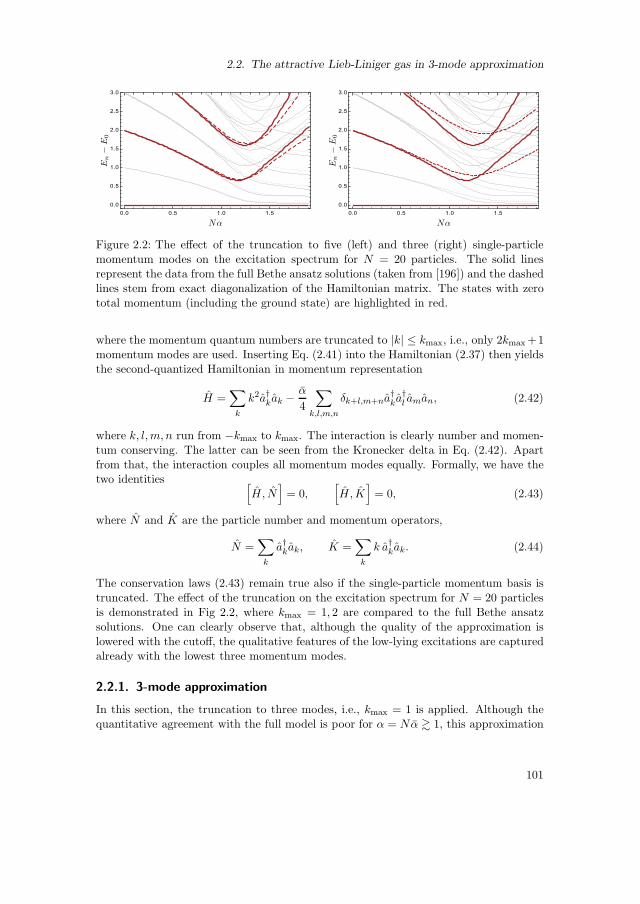
2.2. The attractive Lieb-Liniger gas in 3-mode approximation
Figure 2.2: The effect of the truncation to five (left) and three (right) single-particlemomentum modes on the excitation spectrum for N = 20 particles. The solid linesrepresent the data from the full Bethe ansatz solutions (taken from [196]) and the dashedlines stem from exact diagonalization of the Hamiltonian matrix. The states with zerototal momentum (including the ground state) are highlighted in red.
where the momentum quantum numbers are truncated to |k| ≤ kmax, i.e., only 2kmax +1momentum modes are used. Inserting Eq. (2.41) into the Hamiltonian (2.37) then yieldsthe second-quantized Hamiltonian in momentum representation
H =∑
k
k2a†kak −α
4
∑
k,l,m,n
δk+l,m+na†ka
†l aman, (2.42)
where k, l,m, n run from −kmax to kmax. The interaction is clearly number and momen-tum conserving. The latter can be seen from the Kronecker delta in Eq. (2.42). Apartfrom that, the interaction couples all momentum modes equally. Formally, we have thetwo identities [
H, N]
= 0,[
H, K]
= 0, (2.43)
where N and K are the particle number and momentum operators,
N =∑
k
a†kak, K =∑
k
k a†kak. (2.44)
The conservation laws (2.43) remain true also if the single-particle momentum basis istruncated. The effect of the truncation on the excitation spectrum for N = 20 particlesis demonstrated in Fig 2.2, where kmax = 1, 2 are compared to the full Bethe ansatzsolutions. One can clearly observe that, although the quality of the approximation islowered with the cutoff, the qualitative features of the low-lying excitations are capturedalready with the lowest three momentum modes.
2.2.1. 3-mode approximation
In this section, the truncation to three modes, i.e., kmax = 1 is applied. Although thequantitative agreement with the full model is poor for α = Nα & 1, this approximation
101

2. A semiclassical treatment of quantum critical phenomena
contains all the physics for understanding the quantum phase transition and its precur-sors for α > 1 and is thus commonly used to study finite size effects in the attractiveLL model [16, 153, 194, 196]. Moreover, it is also of direct experimental relevance, as itcan be essentially realized in a spin-1 BEC, where the spatial degrees of freedom arefrozen out and the dynamics is only in the spin degrees of freedom [201–204]. There, onecan easily control the “kinetic” energy that is actually given by the quadratic Zeemanshift by varying the magnetic field, thus effectively changing the relative strength of thecoupling.
From the theoretical perspective, the three-mode approximation is special, as the twoconstants of motion, namely the particle number N and the total momentum K, allowfor a complete characterization of all states in terms of the latter, while the remainingdegree of freedom is effectively one-dimensional, giving rise to a regular spectrum in eachsector of fixed momentum and particle number. The implications of the two constants ofmotion are clearer when looking at the (classical) mean field limit. There, they lead tointegrable dynamics that, due to the simple analytic form of N and K, can be directlyrepresented in a two-dimensional section of phase space and one-dimensional dynamics.The detailed treatment of the classical limit and its quantization have been performedin [61] and the reader is referred there for details. Here, only the most important stepsare reviewed and additional calculations are given. One important note has to be madeconcerning the presentation of this section: all the results from exact diagonalization ofthe 3-mode model that were used in [61] and [60] have been provided by the author ofthis manuscript. For this reason, some of the figures were created in close collaborationand reappear here without further reference.
2.2.2. Semiclassical treatment
In order to obtain the classical mean-field dynamics, the operators are translated intotheir Wigner symbols as phase space functions. This is done by bringing all productsof operators in symmetric order, leading to additional terms due to the commutationrelations, and then replacing them by classical variables,
ak 7→ φk =qk + ipk√
2=
√nke−iθk , a†k 7→ φ∗k =
qk − ipk√2
=√nkeiθk . (2.45)
The coordinates qk and pk are called quadrature variables [205] and are analogous to theposition and momentum of a harmonic oscillator, but have to be considered only as apair of canonical variables as they are not a physical momentum or position of anything.The polar coordinates nk and θk are related to the quadrature variables by a canonicaltransformation, but do not have an exact quantum analogue. This is, however, onlyimportant when the Maslov indices (c.f., section 2.1.4) are concerned, as they originatefrom the non-commutativity of the quantum operators. The reader is referred to [61] formore details on this issue and for the intermediate steps in the derivation of the classicalHamiltonian function. The classical analogues of the particle number N and the totalmomentum K are given by
Ncl = N − 3
2, N = n−1 + n0 + n1, Kcl = n1 − n−1, (2.46)
102

2.2. The attractive Lieb-Liniger gas in 3-mode approximation
and can be easily shown to be constants of motion of the classical system. After a pointtransformation to the variables N , Kcl and n0 the classical energy per particle can bewritten in scaled variables as
E
N= ω(ϕ, z) + α
(
−1
4+
3
2N− 9
8N2
)
− 1
N, (2.47)
where the classical dynamics is fully determined by
ω(ϕ, z) = 1 − z − α
8
[
(1 − z)(3z + 1) + 4z√
(1 − z)2 − l2 cos 2ϕ]
, (2.48)
with α = αN and the phase space coordinates
z =n0
N, ϕ = θ0 −
1
2(θ1 + θ−1) , ϕ, z =
1
N. (2.49)
In (2.48), the momentum l = Kcl/N enters only as a parameter, while the classicalanalogue to the particle number Ncl, Eq. (2.46), appears only as an effective quantumof action ~eff = 1/N in the Poisson bracket defined by ϕ and n0,
f, g =∂f
∂ϕ
∂g
∂n0− ∂f
∂n0
∂g
∂ϕ, (2.50)
while the classical equations of motion are independent of it,
ϕ =∂ω
∂z, z = −∂ω
∂ϕ. (2.51)
The full EBK quantization of the three-torus then yields the quantization rules
N = N +3
2, N = 0, 1, . . . , (2.52)
Kcl = K, K = 0,±1, · · · ±N (2.53)
for the particle number and the momentum and the numbers N and K can be iden-tified as the eigenvalues of the respective quantum operators. With this, the relationbetween the different definitions α = N α and α = Nα (the natural choice for numericalcalculations) of the coupling can be given as
α =N
Nα =
(
1 +3
2N
)
α. (2.54)
The distinction is not important in the mean field limit but should be accounted forwhen finite size effects are considered.
As the rest of the semiclassical analysis concentrates on the zero-momentum sectorthat contains the ground state, let us setK = 0 in the following. With this, the remainingquantization rule is simplified to
I(ω) =1
2π
∮
dϕ [1 − z(ω,ϕ)] =m+ 1
2
N, m = 0, 1, . . . , ⌊N/2⌋, (2.55)
103

2. A semiclassical treatment of quantum critical phenomena
Figure 2.3: Phase space portrait of the energy ω(z, ϕ), Eq. (2.56), for different valuesof the coupling α. The variable z denotes the relative occupation of the noninteractingground state and ϕ is the conjugate angle. For α > 1, a global energy minimum (cross)and a separatrix (red) connecting two hyperbolic fixed points (dots at z=1) appear. Graylines represent the orbits (tori) that fulfill the quantization condition (2.55) for N = 20.Note that the quantized orbits change their character sequentially.
where z(ϕ,ω) can be obtained from inverting the simplified energy per particle for l = 0,
ω(z, ϕ) = (1 − z)
1 − α
[1 − z
8+ z cos2 ϕ
]
. (2.56)
Figure 2.3 shows the phase space plot of the energy ω(ϕ, z) with the contour lines definedby the quantized energies obtained from the condition (2.55). It involves different typesof classical trajectories following lines of constant energy in phase space with periodicityϕ 7→ ϕ + π. For α < 1 all trajectories are deformed horizontal lines (rotations). Forα > 1 an island centered around a new minimum energy fixed point emerges with orbitsvibrating in ϕ, similar as for the pendulum. This goes along with the formation of aseparatrix at E = Esep (ω = 0) associated with two hyperbolic fixed points at z = 1 andcos2 ϕ = 1/α, characterized by (in)stability exponents
λ(1,2)s = 2√α− 1 ≡ λs. (2.57)
The energy levels that one obtains from the quantization rule (2.55) turn out to bein perfect agreement with the quantum mechanical results obtained from exact diag-onalization of (2.42), as seen in Fig. 2.4 for N = 200 particles, where the excitationenergy dependence with the coupling α is shown for the interesting regime around thecritical point α = 1. To show that also the ground state energy is correctly captured,the exact ground state has been used as a reference in both results, as can be seen inthe inset, where a closeup of the region around α = 1 is shown, revealing small errorsclose to the point where the quantized orbits cross the separatrix. The latter points are
104

2.2. The attractive Lieb-Liniger gas in 3-mode approximation
Figure 2.4: Comparison of the excitation spectrum obtained from exact diagonalization(dots) and semiclassical quantization (lines). In both cases, the exact ground stateenergy has been used as a reference. The dashed line shows the energy of the separatrixwith respect to the ground state, indicating the points where the quantized orbits crossthe separatrix.
indicated by the intersection of the respective levels with the dashed line, that shows theseparatrix energy (with respect to the ground state) defined by ω = 0. As it was alreadyseen from the phase space portraits in Fig. 2.3, the quantized orbits cross the separatrixsuccessively, and the transition for the ground state does not occur at the mean fieldvalue α = 1 for finite particle numbers. This is again verified in Fig. 2.4, where thedashed line starts only at a coupling α ≈ 1.07 > 1. This also leads to a position of theminimal gap Egap between the ground and first excited state that is shifted to a valueαgap = 1 + ∆αgap that is larger than the critical interaction. As one approaches themean field limit N → ∞, the gap energy and the deviation ∆αgap from the critical pointapproach zero in a power law behavior, and the respective exponents can be obtainedfrom an asymptotic analysis of the quantization condition (2.55) [61]8. This asymptoticgap closing is a clear evidence of a quantum phase transition that emerges in the meanfield limit. However, one can clearly see that the transition of the excited states fromone side of the separatrix to the other goes hand in hand with a bunching of levels.This suggests that the gap closing is not a feature unique to the ground an first excitedstate but happens also between higher neighboring states. This can be verified in theexcitation spectrum, where a closer analysis of the semiclassical quantization yields alogarithmic divergence in the inverse level spacing, indicating an excited state quantumphase transition [206]. For a direct evidence of the phase transition, that also givessome insight to the physics behind it, one can calculate the derivatives of the energylevel with index k with respect to the interaction and look for non-analytic behavior.
8The constant prefactors turn out to have the wrong value in this approach, as the relevant phase spaceis rescaled in this limit to stay at the gap. This was corrected by reintroducing quantum operatorsin a local description in [61].
105

2. A semiclassical treatment of quantum critical phenomena
Figure 2.5: Emerging non-analytic behavior in the pair correlation function calculatedin the kth interacting excited state. Note the different scales on the horizontal axis forthe different particle numbers N .
Let us for a moment forget about the approximation introduced by the truncation tothree modes. By means of the Hellmann-Feynman theorem applied to the Hamiltonian(2.37) and using the homogeneity of the system one obtains the relation
d
dαEk(α) = −π
2
∫ 2π
0dθ 〈ψk|Ψ†(θ)Ψ†(θ)Ψ(θ)Ψ(θ)|ψk〉 = −N
2
4g(k)2 (α), (2.58)
where the α-dependence of the kth excitation eigenstate |ψk〉 has been omitted and
g(k)2 (α) =
〈ψk|Ψ†(θ)Ψ†(θ)Ψ(θ)Ψ(θ)|ψk〉(N/2π)2
(2.59)
is the local pair correlation function normalized with the particle density, describing theprobability for finding two particles at the same point. By switching to the parameter
α = Nα and abusing the notation by using the same symbols Ek(α) and g(k)2 (α) for the
functions expressed in terms of α one gets
d2
dα2Ek(α) = −N
4
d
dαg(k)2 (α). (2.60)
The truncation does not change the calculation, but the field operators have to betruncated to three modes, such that they cannot resolve a single point on the ring.
Still, an increase of the function g(k)2 can be interpreted as a sign of particles bunching
together, as it is known to happen for the ground state of the full model. If one is not
comfortable with the interpretation in terms of correlations, one can also view g(k)2 as
the interaction energy per particle
g(k)2 (α) = − 4
αN
(
Ek(α) − 〈ψk(α)|H0|ψk(α)〉)
, (2.61)
106

2.2. The attractive Lieb-Liniger gas in 3-mode approximation
where H0 is the noninteracting Hamiltonian of the noninteracting system. Figure 2.5
shows the numerically obtained (discrete) derivative of g(k)2 (α) for the ground state and
three different excitations and increasing particle numbers, clearly showing a suddenincrease at successive “critical” interaction values, that coincide exactly with the pointswhere the respective quantized orbits cross the separatrix. When increasing the particlenumber, the step gets more narrow, approaching a discontinuity in the pair correlation.This is a clear indication of a second order quantum phase transition of the ground and
the excited states that manifests itself in the mean field limit. Moreover, this showsthat the excited state quantum phase transitions have their origin in the presence of theseparatrix in the mean field description. This means that, when tuning the interactionbeyond the critical value α = 1, there will always be states that correspond to quantizedorbits close to or at the separatrix, thus yielding critical states for any such interactionin the mean field limit. This will play an important role later, when these states turn outto be of central relevance for the quantum dynamics in certain quench scenarios. Thereis one interesting result that was not mentioned explicitly up to now: Even though thereis no phase transition for finite particle numbers, one can now define a precise finite-sizecritical coupling for every state given by the condition that the state corresponds to thequantized separatrix. There, in the classical picture, the orbit changes discontinuously
form a vibration/libration to a rotating orbit.
Separatrix dynamics
A general semiclassical analysis, that is valid for any situation, where a classical anal-ysis yields isolated hyperbolic fixed points in an effective two-dimensional phase space,has shown [60], that the quantization of orbits that come close to these paths yield alogarithmic divergence of the mean density of states. One can get a good intuition onwhy this happens by noticing that a quantization condition of the form
I(E) =(
n+ν
4
)
~eff , (2.62)
with n labeling the excitation of the states, can be interpreted on a smooth level asthe equation for the integrated density of states. Solving for the level index n anddifferentiating with respect to the energy yields
ρ(E) =1
~eff
dI(E)
dE=T (E)
~eff, (2.63)
i.e., the smooth level density is determined by the time period of the quantized orbit.This (classical) time diverges logarithmically when a hyperbolic fixed point is approachedand any orbit that is close enough to a separatrix will come close to at least one suchfixed point. Therefore, the level density will be dominated by those points through theirlogarithmically diverging time contributions.
For the three-mode approximation the calculations yields
ρ(E) ≈ 1
2πλlog
( |E − Esep|N
)
+ O(
N0)
(2.64)
107

2. A semiclassical treatment of quantum critical phenomena
with λ given by the sum of reciprocal (in)stability exponents along the way,
λ =
(∑
FP
λ−1FP
)−1
=λs2
=√α− 1. (2.65)
The second equality sign uses that the stability exponents λs, Eq. (2.57), are the samefor the two hyperbolic fixed points of the three-mode model. By using the quantizationrule (2.62) beyond the smooth level, one obtains a set of states around the separatrixwith an asymptotically constant level spacing that scales as [61,189]
∆E ∼ 2π√α− 1
log N(2.66)
thus setting a unique time scale for superpositions of the respective states given by theinverse spacing
τ =2π
∆E=
1
λlog N + O
(
N0)
. (2.67)
It is important to note that the level spacing (2.66) is only valid for a number of statesthat grows sub-algebraic with the particle number (or the inverse effective Planck con-stant) [61]. Remarkably, the timescale (2.67) has exactly the form of the Ehrenfesttime
τE =1
λLlog(scl~
)
(2.68)
defined in chaotic systems. In (2.68), λL is the Lyapunov exponent and scl is a typicalclassical action. So, the effective time scale τ can be obtained from the Ehrenfest timeby substituting the Lyapunov exponent by (half of) the stability exponent and using theeffective action scl = 1 together with the effective Planck constant ~eff = 1/N . For thisreason the time scale τ , Eq. (2.67), is further referred to as the local Ehrenfest time.
The WKB wave functions
The EBK quantization summarized above relies on the detailed knowledge of the topol-ogy of the phase space, i.e., one has to find the action-angle variables that characterizethe (degenerate) three-torus where the motion takes place. This information is then cru-cial for the determination of the Maslov index. However, the action-angle variables donot have a quantum analogue so that the actual WKB wave functions should be definedin the original coordinates qk (or pk), yielding a wave function that depends on threecoordinates. But this would be a very complicated task as one would have to find the full(multi-valued) action that wraps around the torus. Moreover, the natural basis of thequantum system is given by the Fock states (with three modes) that have a fixed particlenumber N and zero momentum, and thus can be labeled by the zero-mode occupationor occupation fraction. The latter is the quantum analogue of the variable z, so thatdefining the semiclassical WKB wave functions in the qk looks like an unnecessary de-tour. However, the number operator n0 = a†0a0 does not have an exact conjugate “phaseoperator”. The reason for this can be found in the periodicity of the phase together
108

2.2. The attractive Lieb-Liniger gas in 3-mode approximation
with the lower-boundedness of n0. In the semiclassical limit, it is however legitimateto assume that any pair of conjugate classical variables locally corresponds to conjugatequantum operators and that in the case of the action-angle variables, where the actionsare constants of motion and thus exactly fixed, the WKB wave function expressed in theangles has to look like a plane wave locally. Now, as the particle number and the totalmomentum (which can be negative) are closely related to two of the action variables,one can expect that using the action defined only in the two-dimensional phase spacespanned by z and ϕ should yield good results.
The wave functions will only be given for the rotations here, but it is expectedthat the vibrations can be treated similarly. Let us start with the definition of theϕ-representation of the Fock states with fixed momentum and particle number,
|m〉 ≡∣∣∣∣
N −K −m
2,m,
N +K −m
2
⟩
, (2.69)
where the positions stand for the occupations of the k = −1, 0, 1 modes in this orderand m has the same parity as N ±K. For K = 0 this simplifies to the symmetric states
|m〉 =
∣∣∣∣
N −m
2,m,
N −m
2
⟩
, m = N − 2j (2.70)
with 0 ≤ j ≤ ⌊N/2⌋ being an integer. One can then define a ϕ representation as
〈ϕ|m〉 =1√2π
eiϕm, 0 ≤ ϕ < 2π (2.71)
using the states
|ϕ〉 =∑
me−imϕ |m〉 (2.72)
that form an overcomplete basis in the sector of the three-mode Fock space with fixedparticle number and momentum spanned by the states (2.70). In particular we have
∫ 2π
0|ϕ〉 〈ϕ| = 1, (2.73)
〈ϕ′|ϕ〉 =1
2πei(N−⌊N/2⌋)(ϕ′−ϕ) sin [(⌊N/2⌋ + 1)(ϕ′ − ϕ)]
sin(ϕ′ − ϕ), (2.74)
i.e., the states are not orthogonal and thus cannot be eigenstates of a hermitian operator.The semiclassical WKB wave functions for the rotations with quantum number n can
then be defined as
ψn(ϕ) ≡ 〈ϕ|ψn〉 =1√2π
∣∣∣∣
∂2Sn(ϕ)
∂ϕ∂J
∣∣∣∣
12
eiNSn(ϕ)−if(ϕ), (2.75)
where the action Sn(ϕ) is given by
Sn(ϕ) =
∫ ϕ
0dϕ′z(ωn, ϕ
′) (2.76)
109

2. A semiclassical treatment of quantum critical phenomena
and the action variable J is given by
J(ω) =1
2π
∫ 2π
0dϕ z(ω,ϕ) = 1 − 2n + 1
N, (2.77)
where the second equality is the original quantization rule applying for the rotationsonly [61]. It is related to the common action variable I for both types of motion, (2.55),by J = 1 − 2I. The function f(ϕ) in (2.75) was introduced to assure the periodicity ofthe wave function, i.e., it compensates the Maslov index ν = 2 coming from two (hidden)turning points [61] such that the function f(ϕ) should fulfill
f(ϕ+ 2π) = f(ϕ) + π. (2.78)
In the noninteracting limit α→ 0 one obtains
ψn(ϕ) =1√2π
ei(N−2n+ 12)ϕ−if(ϕ). (2.79)
By matching this to the ϕ-representation of the quantum mechanical states defined in(2.71) (with m = N − 2n) one finds
f(ϕ) =ϕ
2(2.80)
in this limit, i.e., the additional phase is picked up continuously with a constant rate.Although this might not be exactly true for finite couplings, the effect of nonlinearcontributions to f(ϕ) should be subdominant. Using elementary manipulations one canfinally rewrite the WKB wave function for the rotations as
ψn(ϕ) =1√2π
∣∣∣∣
∂z
∂ω
/∂J
∂ω
∣∣∣∣
12
eiNSn(ϕ)−iϕ2 , (2.81)
Where the prefactor has to be evaluated at ω = ωn given by the quantization rule (2.55)or (2.77).
One can get a better intuition of the prefactor by identifying the time period Tn of afull cycle of the quantized orbit and the (phase) velocity vn along the trajectory as
Tn = 2π
∣∣∣∣
∂J
∂ω
∣∣∣∣ωn
=
∫ 2π
0dϕ
1
vn(ϕ), vn(ϕ) =
∣∣∣∣
∂z
∂ω
∣∣∣∣
−1
ωn
. (2.82)
With this, the semiclassical WKB wave function is conveniently written as
ψn(ϕ) =eiNSn(ϕ)−iϕ
2
√
Tnvn(ϕ). (2.83)
Also, it is clear from (2.82) that the wave function is normalized to one. From Eq. (2.83)one can directly identify situations, where the WKB wave function will not be well-behaved: First, the classical velocity vn is zero at turning points, leading to a divergence
110
2.2. The attractive Lieb-Liniger gas in 3-mode approximation
of the wave function. Second, the velocity becomes very small if the orbit comes closeto a hyperbolic fixed point, such that the probability density |ψn(ϕ)|2 is strongly peakedaround small regions around the hyperbolic fixed points, reflecting the fact that a clas-sical “particle” would be in these regions of phase space most of the time (borrowingthe intuition from the single-particle picture for a moment). As we will see later, thesemiclassical description is less accurate in these situations.
To be able to directly compare the WKB wave function (2.83) with the numericalstates one either has to use the ϕ-representation of the quantum states defined above orthe wave function has to be transformed into the Fock basis. As the latter is the naturalbasis of the many-body quantum system, we proceed by calculating the projections
a(n)m = 〈m|ψn〉 of the WKB wave functions as
a(n)m =1√2π
∫ 2π
0e−imϕψn(ϕ) =
1√2πTn
∫ 2π
0dϕ
ei(NSn(ϕ)−ϕ2−mϕ)
√
vn(ϕ). (2.84)
Switching to the action
Sn(ϕ) = ϕ− Sn(ϕ) =
∫ ϕ
0dϕ′ (1 − z(ωn, ϕ
′)) (2.85)
that is closer related to the variable I, (2.55), and writing m = N − 2k then yields
a(n)N−2k =
4√2πTn
∫ π2
0dϕ
1√
vn(ϕ)cos(
N Sn(ϕ) − (2k + 1)ϕ)
. (2.86)
Here, the identity Sn(ϕ+π) = Sn(ϕ)+2πI, that follows from the π-periodicity of z(ωn, ϕ)in ϕ, and leads to a π-periodicity of the exponential, as well as the antisymmetry of theexponent with respect to ϕ = 0 have been used.
Before comparing the semiclassical with the exact quantum-mechanical results, let usderive a simplified result obtained from evaluating the integral (2.86) in stationary phaseapproximation (SPA). The condition for the stationary phase is given by
z(k)s ≡ z(ωn, ϕ(n,k)s ) = 1 − 2k + 1
N=m+ 1
2
N, (2.87)
with m = N−2k. It describes the point where the quantized orbit crosses the horizontal
line at z(k)s = (m+ 1/2)/N , which are exactly the quantized orbits corresponding to the
noninteracting states. This is true also for overlaps of eigenstates with any two differentcouplings α1 and α2, and leads to a general criterion for a non-vanishing overlap betweenstates: if the corresponding classical orbits cross, they have a finite overlap characterizedby the crossing angle (in SPA), while the overlap is exponentially small otherwise.
In the case at hand we have α1 = α and α2 = 0 and the solution of (2.87) is given by
x(n,k)s ≡ cos2 ϕ(n,k)s =
1
z(k)s
[
1
α
(
1 − ωn
1 − z(k)s
)
− 1 − z(k)s
8
]
. (2.88)
111

2. A semiclassical treatment of quantum critical phenomena
The slope of z(ωn, ϕ) at this point defines the curvature of the action Sn and is given by(omitting the n and k index)
(∂z
∂ϕ
)
ωn,ϕs
= −(∂ω
∂ϕ
)
zs,ϕs
(∂ω
∂z
)−1
zs,ϕs
, (2.89)
where the right hand side is easily calculated from the Hamiltonian function (2.56).However, the second term does not have to be evaluated further, as it can be identifiedas the velocity vn(ϕs) and is canceled in the SPA. Combining the above yields theeigenvector components in SPA
a(n)N−2k ≈
4 cos(
N Sn
(
ϕ(n,k)s
)
− (2k + 1)ϕ(n,k)s − π
4
)
√
Tn × f(k)n
, (2.90)
where, as before, Tn is independent on k and f(k)n is the analogue to vn(ϕ) given by
f (k)n =
(∂ω
∂ϕ
)
zs,ϕs
= 2αz(k)s
(
1 − z(k)s
)√
x(n,k)s
(
1 − x(n,k)s
)
, (2.91)
with z(k)s and x
(n,k)s given in (2.87) and (2.88), respectively.
A few remarks concerning the validity of these results should be made: First, duringthe calculation, one finds that using the depletion of the zero-mode, i.e., 1−z is more nat-ural for the lower excitations, as some highly oscillating terms cancel out. This suggeststhat one could start off directly from the description using ζ = 1− z as a canonical vari-able and defining the quantum states accordingly. For the calculation of the WKB wavefunctions for the vibrations, this approach is probably better suited, as the actions belowand above the separatrix energy are then expected to have a smooth transition. Second,one immediately sees that approaching the noninteracting limit, where the quantizedorbits approach horizontal lines (see Fig. 2.3), the integral in Eq. (2.86) should not be
approximated by a stationary phase approximation. Finally, the vectors (a(n)m ) are not
necessarily normalized, as they are projected to a very specific set of plane waves: Thewavenumbers m = N − 2k in Eq. (2.71) are non-negative, they have a cutoff mcut = N ,and they have the same parity as the particle number N . As the WKB wave function hasexactly the same behavior ψn(ϕ+ π) = (−1)Nψn(ϕ) as the respective plane waves, thelast condition is not a restriction at all, while the cutoffs can have a non-negligible effect.The stationary phase condition gives a good hint on what can happen: if the quantizedorbit crosses the horizontal line at zs = (m + 1/2)/N , the respective wavenumber m isrelevant for the stationary phase analysis. If there is no such crossing, the point withstationary phase bifurcates into two saddle points in the complex plane giving rise toevanescent contributions that drop off exponentially with the distance of from a turningpoint in z. As long as the classical orbit stays away from the phase space boundaries0 ≤ z ≤ 1 (within a distance given by the penetration depth ∼ 1/N of the classicallyforbidden region) one can safely ignore any out-of-bound wavenumbers. Unfortunately,
112

2.2. The attractive Lieb-Liniger gas in 3-mode approximation
Figure 2.6: Comparison of the full semiclassical eigenvectors, Eq. (2.86), (lower panels),and the SPA result, Eq. (2.90), (upper panels), with the exact eigenvectors (green)for N = 200 and α = 2. The curves show the squares of the (real) eigenvectors ofthe respective results. The solid lines connecting the discrete eigenvector componentsare only drawn for better visibility. Left: Excitation with n = 40 well above the theseparatrix energy. The results from the full integration and the exact diagonalizationare indistinguishable (lower panel) while the SPA approximation fails at the turningpoints as expected. Right: Smallest energy eigenstate above the separatrix energy (n =21). The normalization of the semiclassical results deviates from the exact values, butthe overall agreement is still good. Surprisingly, the SPA result is much better thanthe the full integration and can be renormalized such that it fits the numerical resultalmost everywhere (not shown), while the full integration yields larger or smaller valuescompared with the exact vector components depending on k.
when one approaches the separatrix energy, the quantized orbit will be very close to theline z = 1 for both types of motion and the results for the rotational orbits closest to theseparatrix with ω ≈ 0 turn out to be less accurate than the ones with sufficiently largeω > 0, also leading to non-normalized eigenvectors. In all other cases, the normalization
of the a(n)n obtained from the numerical integration of (2.86) are very close to one down
to small particle numbers of the order of N ∼ 10.
There is one further remark that should be made. It turns out that using the SPAresult also in the classically forbidden regime, i.e., at one of the complex saddles, thereal part of the resulting expression leads to the correct evanescent behavior, which isexploited in the figures discussed below.
Let us now turn to the actual comparison of the semiclassical and quantum-mechanicalresults, the latter being obtained from exact-diagonalization of H, Eq. (2.42) withkmax = 1. Figure 2.6 shows the comparisons of the semiclassical eigenvectors fromthe full calculation, Eq. (2.86), and the result in SPA, Eq. (2.90), with the exact eigen-vectors for two different excitations. For the state with n = 40 well above the separatrix(ωn ≈ 0.125), the full semiclassical result is indistinguishable from the exact one, witha normalization that is one to machine precision (approx. 10−16). The SPA fails at theturning points where ∂z/∂ϕ = 0 and can diverge for fine-tuned values of the interac-tion (if a turning point in z coincides with zs for one of the values of k), while it gives
113

2. A semiclassical treatment of quantum critical phenomena
Figure 2.7: The comparison of the semiclassical and quantum mechanical eigenvectorsanalogous to Fig. 2.6. Left: N = 10, α = 1.8, and n = 1 (blue), 2 (orange), and 4 (green).The full full integration of (2.86) still yields good results for n > 1 (lower panel), butthe SPA is not justified anymore and gives poor approximations of the quantum states(upper panel). Right: N = 2000, α = 1.7, and n = 280. Both upper and lower panelshow the semiclassical results (green) above the exact quantum states (red). However,the full semiclassical result completely shadows the latter. Only in the SPA result,deviations can be seen at the classical turning points. This is highlighted in the rightpart of the figure, that shows as closeup of the turning point in z at ϕ = 0, see Fig. 2.3.
perfect results in the central part. For the lowest state above the separatrix energy(n = 21, ωn ≈ 1.27 × 10⁻⁴) both semiclassical results yield a wrong normalization. Thefull integration of Eq. (2.86) gives values that are too small or too large depending onthe value k and thus will not be much improved by renormalization. This is probablyalso connected to the fact that the semiclassical quantization is not perfect close to theseparatrix, and ωn deviates from the exact value ωn ≈ 1.62 × 10⁻⁴ in the case at hand.Surprisingly, the SPA result is much more accurate and can be renormalized such thatit coincides with the exact result everywhere except at few values around the turningpoints. This might be due to the fact that the ϕ representation of the WKB wavefunction has a divergence at the hyperbolic fixed points, i.e., for ω = 0 and that thisdivergence strongly affects all the integrals, while the divergent term is absent in the SPAresult, that is only determined by the crossing points of the quantized orbits with thehorizontal lines and is thus insensitive to the hyperbolic fixed point almost everywhere.
For small particle numbers, i.e., a large effective Planck’s constant, the semiclassi-cal result and especially the SPA are expected to be poor approximations. Figure 2.7demonstrates the effect of small and large particle numbers on the results. As it turnsout, the full semiclassical result is still very good even for N = 10 (left part of the figure),as long as one is far enough above the separatrix energy. However, the stationary phaseapproximation does not give good results and cannot be justified anymore. The rightpart of Fig. 2.7 shows the comparison of the results for N = 2000. As expected, thesemiclassical approximations give essentially exact results, except for the SPA divergingat the classical turning points as is typical for WKB wave functions, but can be fixed bymeans of uniform approximations [42].
114
2.2. The attractive Lieb-Liniger gas in 3-mode approximation
To conclude, the semiclassical WKB wave function defined in the angle-representationfor the rotating classical orbits captures essentially the full quantum state even downthe few-particle case, as long as its energy is well above the separatrix energy. There,using the exact projection to the noninteracting states, one can obtain the full quantummechanical eigenstates in the Fock basis, also capturing the transition from oscillatory toevanescent behavior at the turning points (in the condensate fraction z) of the quantizedorbits. Moreover, the resulting states are correctly normalized.
Away from the classical turning points in z, the SPA works equally well for largeparticle numbers, however giving rise to the typical breakdown close to them.
One drawback of the WKB wave functions introduced here is that they cannot beused to extract the overlap of the states close to the separatrix energy with the low-lyingnoninteracting states that play an important role in quench scenarios. One way out ofthis dilemma could be a requantization of a local description around the hyperbolic fixedpoints as was used for the analysis of the fundamental gap between the ground stateand the first excited state [61].
2.2.3. Phase space representation: Husimi functions
The semiclassical WKB wave functions investigated so far are analytic approximationsto the actual quantum states. One can, however, directly visualize the quantum states byusing one of the phase-space representations, i.e., the Wigner, Husimi Q and GlauberSu-darshan P distributions [156]. Here, due to its simple computability, the Husimi functionis calculated for the exact quantum states. For this one first has to calculate the coherentstates in the 3-mode model. They are given in normalized form by
|α−1α0α1〉 = e−12(|α−1|2+|α0|2+|α1|2) eα−1a
†−1+α0a
†0+α1a
†1 |0〉 , (2.92)
where |0〉 is the vacuum state and the αi = qi + ipi are complex numbers. One caneasily show that the expectation values for the particle number and the momentum in acoherent state are given by
〈N 〉 = |α−1|2 + |α0|2 + |α1|2 ≡ N , 〈K〉 = |α1|2 − |α−1|2 ≡ K. (2.93)
Coherent states are superpositions of Fock states with different total particle number Nand momentum K. The Husimi function is however given by the expectation value
Qρ(α−1, α0, α1) =1
π3〈α−1α0α1|ρ|α−1α0α1〉 (2.94)
of the density matrix of the quantum state that can (and should) be chosen to havefixed N and K. So, only the information of the projections of the coherent states tospecific particle numbers and momenta is used. But these projections actually allowfor a parametrization using only four independent variables, one of them being only arenormalization, such that the quantum state can be represented in a tree-dimensionalsubspace of the six-dimensional phase space spanned by the αi.
115
2. A semiclassical treatment of quantum critical phenomena
Let us denote the projection of the coherent state to the sector of Fock space with Nparticles and momentum K by
|α−1α0α1〉N,L = PN,L |α−1α0α1〉 , (2.95)
where PN,L is the projector to the respective subspace. The full coherent state is thenjust the sum of the projected states.
By expanding the projected state into Fock states, changing to polar coordinatesαi =
√nie
iϑi , and expressing it in terms of the expectation values N and K, Eq. (2.93),one finds that the fixed particle number and momentum lead to the U(1) symmetries intwo of the angles, i.e., two of the angles contribute only a phase, such that the projectedcoherent state is given by
|α−1α0α1〉N,K = eiNϕN+iKϕK [PN (N)]12 |z, ϕ, l〉N,K , (2.96)
where the new angles and scaled parameters z and l are given by
ϕ = ϑ0 −ϑ1 + ϑ−1
2, ϕN =
ϑ1 + ϑ−1
2, ϕK =
ϑ1 − ϑ−1
2(2.97)
and
z =n0N
∈ [0, 1], l =K
N∈ [−(1 − z), 1 − z]. (2.98)
This is in complete analogy to the transformations that are used to eliminate the con-stants of motion in the classical analysis of the 3-mode model, thus the individual stepsare not repeated here. The function PN (N) in Eq. (2.96) is the Poisson distribution ofthe number N with parameter N and reflects the probability distribution of the particlenumber N in the coherent state. As the phases and the normalization with the Poissondistribution do not have a physical meaning, the projected coherent state is reduced toa superposition of coherent single-particle excitations
|z, ϕ, l〉N,K =1
2π√N !
∫ 2π
0dθ eiKθ
[
bz,ϕ,l(θ)†]N
|0〉 , (2.99)
with the parametrized single-particle modes
bz,ϕ,l(θ) =
√
1 − z − l
2e−iθa−1 +
√ze−iϕa0 +
√
1 − z + l
2eiθa1. (2.100)
The integration over the angle θ has only been introduced to simplify the notation andensures the correct total momentum K of the state. The states (2.99) are not normalizedto one but they fulfill the completeness relation (omitting the index N,K on the states)
(N + 2)(N + 1)
2π
∫ 1
0dz
∫ π
0dϕ
∫ 1−z
−(1−z)dl |z, ϕ, l〉 〈z, ϕ, l| = PN,K , (2.101)
116

2.2. The attractive Lieb-Liniger gas in 3-mode approximation
i.e., they form a complete basis on the sector with particle number N and momentumK. With this, one can define the normalized Husimi Q representation of the states withfixed particle number N and fixed momentum K as
Q(N,K)ρ (z, ϕ, l) =
(N + 2)(N + 1)
2π〈z, ϕ, l|ρN,K |z, ϕ, l〉 (2.102)
for a density matrix with fixed particle number and momentum.
To obtain a two-dimensional representation one has to either trace out the phase spacevariable l associated with momentum or look at fixed values of l. As one might expect,the phase space density in l obtained from tracing out z and ϕ then peaks at l = K/Nwith the peak getting more pronounced with higher N . It is thus reasonable to expectthat using this value for a projection will contain most of the physics. This approachis used in the following, however with a modification. First, one defines the normalizedcoherent states as
|z, ϕ〉l ≡ c(z, l) |z, ϕ, l〉 (2.103)
with
|c(z, l)|−2 =1
2π
∫ 2π
0dθeiKθ
[1 − z − l
2eiθ + z +
1 − z + l
2e−iθ
]N
(2.104)
and then numerically checks, whether these states have a completeness relation. Thisyields, using K > 0 for simplicity,
∫ 1−l
0dz
∫ π
0dϕ |z, ϕ〉 〈z, ϕ| =
⌊N−K2
⌋∑
k=0
ak(l) |k〉 〈k| , (2.105)
where the states |k〉 are the three-mode Fock states with occupations n−1 = k, n1 =k + K, and n0 = N − K − 2k, that span the sector with fixed particle number andmomentum. One then finds numerically that th coefficients ak(l) are almost uniformfor l = K/N such that the states |z, ϕ〉K/N form an (almost) complete set and (2.105)
is approximately proportional to the projection operator PN,K , with the approximationgetting better with higher particle numbers, as expected.
Figure 2.8 shows the Husimi functions obtained in this way for N = 100, K = 0, andα = 1.9. The left figure shows four different eigenstates, starting from the ground statewith index k = 0 being localized at the classical energy minimum. The state with k = 3then resembles a vibrational orbit while the state with k = 9 is energetically close to theseparatrix in classical phase space and shows signatures of both kinds of classical orbits.Higher excitations (k = 15 is shown) clearly have the signature of rotational classicalorbits. The right part of Fig. 2.8 shows the time evolution of the noninteracting groundstate after a quench of the interaction to α = 1.9. The time is given in units of the [finite-size corrected, see Eq. (2.141)] local Ehrenfest time scale τ , Eq. (2.67). The distributionfirst approaches the region where one of the classical fixed points is located, then followsthe lower branch of the separatrix and comes back very close to the initial distribution
117

2. A semiclassical treatment of quantum critical phenomena
Figure 2.8: Plots of the Husimi functions for N = 100 and α = 1.9. In each plot, thevalues of z range from 0.3 to 1 and the values of ϕ range from −π/2 to π/2. Left: thekth eigenstates for k = 0, 3, 9, 15. Right: Time evolution of the noninteracting groundstate after a quench to the coupling α = 1.9 for times t = 0, 0.4τ, τ, 1.4τ , showing arevival of the initial state at t ≈ τ . For t = 1.4τ , interference can be seen, as a part ofthe wave packet is split off.
at t = τ . However, this revival is not perfect and one can see interference effects at latertimes, where a small part of the wave packet splits off (see plot for t = 1.4τ). Also,the distribution is stretched stronger than one “period” before at t = 0.4τ . However,one can still observe large parts of the distribution being concentrated at the boundaryz = 1 for multiples of τ (not shown), which leads to the oscillations in the one-bodyentropy found in [61]. The implications of these oscillations for the out-of-time-orderedcorrelator are investigated in the next section.
2.2.4. The out-of-time-ordered correlator close to criticality
In this subsection, a specific quench scenario is applied and the subsequent non-equilib-rium time dynamics is studied. As has been mentioned above, the semiclassical quan-tization around the separatrix gives rise to a very specific local level spacing given (toleading order in N) by
∆Esep ≈ 2π√α− 1
log N. (2.106)
This scaling is however only valid for a certain number of states where the classicaldynamics is dominated by the vicinity of the hyperbolic fixed points. It turns out that thelow-lying noninteracting states have exactly this property. Thus, if the noninteractingsystem is prepared at very low temperatures and the interaction is then quenched to afinite value α > 1, the subsequent time dynamics will be strongly dominated by the localEhrenfest time τ , Eq. (2.67). This has been verified in [61] for the reduced one-bodydensity matrix, where increasing the particle number has led to a quasi-periodic timeevolution of the von Neumann entropy calculated from the time evolution of the reduceddensity matrix. As it turns out, the conservation of the momentum renders the reducedone-body density matrix diagonal, and the only nontrivial dynamics is captured by the
118
2.2. The attractive Lieb-Liniger gas in 3-mode approximation
time evolution of the mean condensate depletion that undergoes distinct oscillationsthat have also been found experimentally in the spin-1 Bose gas [204]. Here, the moreintricate evolution of a certain OTOC will be studied and discussed.
The OTOC that is used here is defined by the expectation value of the squared com-mutator of the condensate fraction n0/N at different times:
C(t) = −N−4 〈Ψ|[n0(0), n0(t)]2|Ψ〉 . (2.107)
Here, n0 = a†0a0, and the expectation value is taken with respect to the noninteracting
condensate |Ψ〉 = 1/√N !(a†0)N |0〉, with |0〉 being the vacuum state. The operator choice
in Eq. (2.107) is the simplest nontrivial choice of operators in this model and it is worthnoting that, due to the conservation of particle number N and momentum K, Eq. (2.44),and [n0(t), N ] = [n0(t), K] = 0, the seemingly more general definition of the OTOC
Cij(k) = −N−4 〈Ψ|[ni(0), nj(t)]2|Ψ〉 , i, j ∈ −1, 0, 1, (2.108)
is completely equivalent to (2.107), i.e., one has
Cij(t) = cij C(t) (2.109)
with real constants cij .
Semiclassical short-time analysis of the OTOC
The short-time mean-field (classical) dynamics of the OTOC can be obtained by notingthat the operator n0/N corresponds to the variable z and by taking only the fist non-vanishing order in N−1 (here identifying N ≈ N) yields the phase space average of thePoisson bracket
C(t) ≈ 1
N2
⟨z(0), z(t)2
⟩
PS=
1
N2
⟨(∂z(t)
∂ϕ(0)
)2⟩
PS
, (2.110)
where the average should be taken using the Wigner quasi-distribution function of thecondensate. This is in complete analogy to the considerations in subsection 2.1.5 of theintroduction of chapter 2 with ~eff = 1/N , which is why the steps are not reproducedhere. Note that the Poisson bracket used here is defined by the phase space variables(ϕ, z) instead of (ϕ, n0) [c.f., Eq. (2.50)]. Without calculation, one can now expect thatthe Wigner function of the non-interacting ground state will be exponentially localizedat the upper boundary of the phase space, with a localization length that scales as 1/Nin order to be compatible with the quantized orbit z = 1/N that exactly reproducesthe ground state in EBK torus quantization. This is also supported by the WKB wavefunction analysis presented earlier in this section, where the overlap of the interactingstates with the noninteracting condensate was exponentially small if the correspondingquantized orbits did not meet, such that only the classical phase space close to theupper boundary can contribute to the quantum-mechanical short-time dynamics thatare described by the truncated Wigner-like approach taken here.
119
2. A semiclassical treatment of quantum critical phenomena
With this line of arguing, only the classical dynamics close to the separatrix play a rolefor short times. There, the hyperbolic fixed points dominate the dynamics, introducingan exponential sensitivity to changes in the initial conditions with a divergence rate givenby the stability exponent λs of the fixed points. One can thus expect C(t) to behave like
C(t) ≈ c
N2e2λst (2.111)
for short times, with a constant c that is to be determined. This is indeed true, butthere is one crucial point that was skipped in the arguments. The dynamics around ahyperbolic fixed point is actually decoupled such that for a trajectory starting close tothe fixed point one obtains
z(t) = z(0)e±λst ⇒ ∂z(t)
∂ϕ(0)= 0, (2.112)
if a local approximation is assumed. This would render those local contributions triviallyzero. Therefore, a closer analysis of the classical dynamics is required that covers thewhole range of relevant initial conditions.
Let us thus approximate the Hamiltonian function for small distances ζ = 1 − z fromthe upper boundary, while keeping the full dependence on ϕ:
ω(ϕ, z) = ζ(1 − α cos2 ϕ). (2.113)
This linear approximation in ζ is only valid if (1− α cos2 ϕ) ≫ ζ. As we are interested inthe case α > 1, where the ϕ-coordinates ϕc of the hyperbolic fixed points are determinedby 1−α cos2 ϕc = 0 this exactly excludes the fixed points. The philosophy of the approachhere is to approximate the classical dynamics away from the fixed point by the linearapproximation in ζ and switching to the local hyperbolic description when the ϕ − ϕc
becomes comparable to ζ, i.e., the fixed point is approached. This can be summarizedin writing
∂z(t)
∂ϕ(0)=
∂z(t)
∂z(tc)
∂z(tc)
∂ϕ(0)≈ eλs(t−tc) × ∂z(tc)
∂ϕ(0)
∣∣∣∣lin
(2.114)
with some intermediate time tc where the linearization breaks down and with the secondfactor evaluated using the linearized Hamiltonian function ω. Here, it has been assumedthat the initial angle ϕ(0) is not at one of the fixed points. Then, the trajectory willapproach the fixed point that is attractive in ϕ and thus repulsive in ζ. Therefore, onlythe diverging solution from (2.112) close to the fixed point is used.
Let us now solve the linearized problem with the Hamiltonian function (2.113). Byusing the distance ζ = 1 − z from the boundary as a variable, the equations of motion(2.51) are modified to
ζ =∂ω
∂ϕ, ϕ = −∂ω
∂ζ= α cos2 ϕ− 1 (2.115)
subject to the initial conditions ζ(0) = ζ0 and ϕ(0) = ϕ0. As can be seen, the equationof motion for ϕ completely decouples from ζ. It can be solved by separation as
t(ϕ,ϕ0) =
∫ ϕ
ϕ0
dϕ′
α cos2 ϕ− 1. (2.116)
120

2.2. The attractive Lieb-Liniger gas in 3-mode approximation
Before solving this equation, let us express ζ(t) and its derivative with respect to ϕ0 byϕ(t). For the former, the energy conservation directly yields
ω = −ζϕ ⇒ ζ(t) = ζ(0)ϕ(0)
ϕ(t)= ζ0
α cos2 ϕ0 − 1
α cos2 ϕ(t) − 1. (2.117)
To get the derivative of ζ(t) with respect to ϕ0 one can make use of the general form ofthe solution of (2.116) with
(∂ϕ
∂ϕ0
)
t
= −(∂ϕ
∂t
)
ϕ0
(∂t
∂ϕ0
)
ϕ
= −ϕ(t)
(
− 1
ϕ(0)
)
=ϕ(t)
ϕ(0)=
ζ0ζ(t)
(2.118)
which can be used to evaluate the derivative of ζ(t) with respect to ϕ0, leading to
∂ζ
∂ϕ0
∣∣∣∣lin
= ζ0sin 2ϕ− sin 2ϕ0
cos2 ϕ− α−1, (2.119)
where the explicit time dependence has been suppressed for simplicity. This solutionmust be cut off at a certain distance δ from the fixed point located at ϕc = arccos(1/
√α),
where the solution of (2.116) will end up eventually. We can thus set ϕ = ϕc + δ andexpand the the above result for small δ. To leading order, this yields
∂ζ
∂ϕ0
∣∣∣∣lin
≈ ζ02 cos(ϕ0 + ϕc) sin(ϕ0 − ϕc)
sin(2ϕc)δ−1. (2.120)
The exact solution to (2.116) can be expressed as
sin(ϕ+ ϕc)
sin(ϕ− ϕc)=
sin(ϕ0 + ϕc)
sin(ϕ0 − ϕc)eλst. (2.121)
By expanding also this at t = tc, where tc defines the cutoff ϕ(tc) = ϕc + δ one obtains
e−λstc ≈ 1
sin(2ϕc)
sin(ϕ0 + ϕc)
sin(ϕ0 − ϕc)δ. (2.122)
Finally, combining Eqs. (2.114), (2.120), and (2.122), one obtains the simple formula forthe classical instability
∂ζ
∂ϕ0= ζ0
sin(2(ϕ0 + ϕc))
sin2(2ϕc)eλst. (2.123)
There are two details that have been put under the carpet here. First, although theresult does not depend on tc anymore, the calculation assumes that t > tc for giveninitial conditions, i.e., one has to wait a certain time tc ∼ 1/λs given by Eq. (2.122),until an exponential growth can be expected. Second, if one uses Eqs. (2.121) and (2.120)evaluated at t = tc in (2.114) without further approximation, one finds a prefactor of theexponential that depends on the cutoff δ explicitly. This prefactor has a singular limit forδ → 0: for any finite δ, the prefactor vanishes when the initial angle ϕ0 approaches thecutoff, a property that is not shared by the simple limiting expression (2.123). However,
121
2. A semiclassical treatment of quantum critical phenomena
the initial value ζ0 can be chosen arbitrarily small, such that, although we must haveζ ≪ δ, the cutoff can also become arbitrarily small. Moreover, comparing with thenumerically integrated classical dynamics (not shown), one finds that the result (2.123)gives the correct prediction also for very small cutoffs (after waiting for the exponentialbehavior to set in). One intuitive explanation could be that the trajectory stays closeto the fixed point for a longer time, such that the very small nonlinear contributionshave a longer time to grow to notable size. The actual reason is, however, that thehyperbolic fixed points of the Hamiltonian ω, that is only linear in ζ, have the samestability properties as the original ones and can be transformed to the latter by a localcanonical transformation.
We are now in the position to predict the short-time behavior of the OTOC. However,we need to have an estimate for the Wigner distribution for the noninteracting groundstate. Let us assume that the noninteracting ground state is exponentially localized atz = 1 and uniform in ϕ, i.e., the Wigner function has the form
W0(ϕ, z) =a
πe−a(1−z) (2.124)
with a parameter a ≫ 1, such that the function drops off quickly and is normalized toone (restricting ϕ to an interval of length π). On the other hand, the semiclassical quan-tization rule (2.55) is exact in the free case and gives the quantized orbit correspondingto the ground state as
1 − z =1
N. (2.125)
For this to be consistent with the Wigner function above we have to fix the correctclassical limit by setting
∫ π2
−π2
dϕ
∫ 1
0dz W0(ϕ, z) z = 1 − 1
N⇒ a = N ≈ N. (2.126)
So, as expected, the localization length given by 1/a scales as 1/N . With this, one canestimate the phase space average in Eq. (2.110), assuming that the trajectories stay closeto the hyperbolic fixed points for a time that is long enough that all the initial conditionscan contribute to the exponential. This cannot be guaranteed for the initial conditionsthat start off close to the other fixed point at −ϕc, where the dynamics slows downexponentially, but these contributions have a vanishing weight in (2.123), thus justifyingthe average
⟨(∂z(t)
∂ϕ0
)2⟩
PS
=
⟨(∂ζ(t)
∂ϕ0
)2⟩
PS
=
∫ π2
−π2
dϕ0
∫ 1
0dζ0W0(ϕ0, 1 − ζ0)
[
ζ0sin(2(ϕ0 + ϕc))
sin2(2ϕc)eλst
]2
=1
N2
e2λst
sin4(2ϕc)=
1
N2
(α
λs
)4
e2λst. (2.127)
122

2.2. The attractive Lieb-Liniger gas in 3-mode approximation
The short-time behavior of the OTOC is thus estimated semiclassically as
C(t) ≈(
α
Nλs
)4
e2λst. (2.128)
So, the OTOC for the interaction quench considered here is expected to grow expo-nentially for short times (with t & 1/λs), and moreover, by a thorough analysis of theclassical phase space, even the proportionality factor has been calculated. However, asin chaotic systems, quantum interference will become important after a certain time. Inchaotic systems, this leads to a saturation regime after the Ehrenfest time. In contrast,in the integrable system at hand, and with the quench of the noninteracting condensateto the supercritical regime, one could expect that the time dynamics will be dominatedby the local Ehrenfest time (2.67) defined by the local level spacing close to the separa-trix energy (i.e., the excited state quantum phase transition). Moreover, as the latter isthe definitional property of the Heisenberg time that sets the timescale for quantum re-vivals, one might expect to see strong oscillations in the OTOC rather than a saturation,even enhanced by the very regular and asymptotically equidistant spectrum.
It is, however, not obvious that only the states close to the excited state quantum phasetransition contribute to the OTOC, and this is certainly not the case for arbitrary longtimes. As the classical phase-space stability analysis can be expected to become invalidquickly after the local Ehrenfest time, the long-time dynamics can only be obtained fromquantum calculations.
Numerical simulation of the OTOC’s dynamics
For the diagonalization of the OTOC (2.107), the states
|n−1, n1, n0〉 , nj = 0, 1, . . . (2.129)
spanning the three-mode Fock space are used. Restricting to the sector with the particlenumber N and total momentum K = 0 one can label the states by a single quantumnumber as
|k〉 = |k,N − 2k, k〉 , k = 0, 1, . . . , ⌊N/2⌋. (2.130)
These states are the energy eigenstates of the noninteracting system with energy Ek =2k, with the condensate state now given by |0〉. The sectors with different K 6= 0 canbe treated similarly, but they are of no relevance here, as the ground state is a zeromomentum state and the operators used in the OTOC are momentum conserving.
The OTOC can then be expanded by inserting the completeness relation between thecommutators as
C(t) = − 1
N4〈0|[n0(t), n0(0)]2|0〉 =
1
N4
⌊N/2⌋∑
k=0
|〈k|[n0(t), n0(0)]|0〉|2
=
(2
N
)4 ⌊N/2⌋∑
k=0
k2 |〈k|n1(t)|0〉|2 , (2.131)
123

2. A semiclassical treatment of quantum critical phenomena
where switching to the operator n1 (that is identical to n−1 in the zero-momentumsector) yields a more natural description using
n1 |k〉 ≡ n |k〉 = k |k〉 . (2.132)
It is thus clear that the central objects that characterize the OTOC are the time-dependent matrix elements
nk0(t) = 〈k|n(t)|0〉 (2.133)
with k > 0, as the case k = 0 does not contribute to the OTOC (2.131). Thus, asnkl(0) ≡ nkl = kδkl and therefore nk0(0) = 0 for k 6= 0, the whole time dynamics of theOTOC is due to the operator n(t) losing its diagonal form. A different interpretationcan be obtained by switching to the Schrodinger picture by introducing the propagator
Klm(t) =⟨
l∣∣∣e−iHt
∣∣∣m⟩
, (2.134)
leading to forward and backward-in-time propagations,
nk0(t) =∑
l,m
K∗lk(t)nlmKm0(t) =
∑
l
Kkl(−t) l Kl0(t). (2.135)
Here, the asterisk denotes complex conjugation. The matrix elements nk0(t) can thusbe understood as a forward propagation of the condensate, then perturbing the state byapplying the number operator n and propagating back in time to a different (noninter-acting) state, which is only possible due to the “perturbation”.
One might think that, although the semiclassical analysis for short times requiredtaking into account the nonlinearities in the equations of motion, quantum mechanicalinterference could still yield nontrivial results in a local description using a Hamiltonian
Hloc = γz2 + ν(zϕ+ ϕz), (2.136)
with real parameters γ, ν, that one would obtain from the quantization of a local de-scription of the fixed points. Note that this Hamiltonian is a variant of the so-calledxp-model that is conjectured to have a close relation to the Riemann zeros [207]. It isstraightforward to show that the propagator for the Hamiltonian (2.136) is given by9
K(z′, z; t) = 〈z′| exp(−iHloct)|z〉 = e−i γνsinh(νt)zz′δ
(
z′eνt2 − ze−
νt2
)
. (2.137)
In other words, any basis state |z〉 is just accelerated away from or to the fixed pointwithout dispersion (depending on the sign of ν), i.e.,
|ψ(0)〉 = |z0〉 =⇒ |ψ(t)〉 = A(t, z0)eνt2 |z0eνt〉 , (2.138)
with a time dependent phase A(t, z0). Identifying z = k/N in the mean-field limit onewould then obtain
nk′k(t) ∝ 〈z′eνt|zeνt〉 ∝ δ(z′ − z), (2.139)
such that the OTOC would become zero in this approximation.
9The derivation was performed using the Feynman path integral. As the propagators for quadraticHamiltonians are well-understood, the proof is omitted here.
124

2.2. The attractive Lieb-Liniger gas in 3-mode approximation
One should thus work either with the full semiclassical approximation for the propaga-tors Kkl as in [177] or with the exact numerical solutions, which requires the calculationof the eigensystem of the interacting Hamiltonian for the time evolution. Here, the sec-ond approach will be taken. As the matrix elements nkl are only needed for l = 0, theycan then be very efficiently calculated by successive multiplications of matrices with asingle vector, where only the matrix for the change between the noninteracting and in-teracting basis is not sparse (but is needed four times). For moderate particle numbersN . 104 this can be done on a normal desktop computer without approximation. If oneneeds to go to higher particle numbers one can do so by truncating both bases in a waythat is inspired by the semiclassical analysis. For this one first uses the fact that thecondensate state |0〉 only overlaps with a number of states around the separatrix thatscales logarithmically with the particle number, such that the time evolution of this staterequires only a few interacting states that lie close to the separatrix. In a phase spacepicture, the Wigner function of the time evolved state will then only be spread alongthe separatrix, dropping off quickly away from it. Now, the application of the numberoperator n could, in principle, smear out this phase-space distribution. However, thehighest order effect in the effective Planck constant is a multiplication of the phase-spacedistribution with z, i.e., a redistribution of the weight, but not changing the shape ofthe Wigner function, such that it is still exponentially small away from the separatrix.One should thus expect that the overlap of the so-obtained state with interacting statesaway from the separatrix is small such that in the overall calculation, only the statesclose to the separatrix play a role.
This way of arguing might sound inconsistent for the following two reasons: First,the Wigner function does not represent the state itself but the density matrix that itdefines. This is cured by the fact that we are actually only interested in the absolutevalues |nk0(t)|2, which can be written as the expectation value via
|nk0(t)|2 = Tr ρ0(t)nρk(t)n , (2.140)
with the density matrices ρk(t) of the time evolved states e−iHt |k〉, such that a Wignermapping is well defined. Second, one should be very careful using an argument based ona small Planck constant in a calculation that aims on the effects beyond the semiclassicalregime. However, one can put the argument in a different way by stating that for any(fixed) time t, the quenched time evolution of the noninteracting states is calculatedexactly (for all k), but the contributions of the interacting states far from the separatrixare projected out in a final overlap calculation, such that they could have been droppedfrom the beginning. Moreover, one sees that only the states |k〉 that have a non-vanishingoverlap with the states close to the separatrix contribute, such that one can introduce acutoff in k, that can be estimated semiclassically from the minimum in z of the separatrix.This cutoff is very efficient for couplings α & 1, where the separatrix is small. However,as it scales linearly with the particle number, it is less important than the cutoff in theinteracting basis, that can be chosen logarithmic in N . The actual number of states thathave to be used has to be determined by varying the cutoff. Figure 2.9 shows the relativeerror ri(t) in the OTOC when the number of states is truncated to Ni = ⌊i logN⌋ for
125

2. A semiclassical treatment of quantum critical phenomena
Figure 2.9: The relative error in the OTOC when using only Ni = ⌊i logN⌋ energyeigenstates around the separatrix energy. The left three plots show the error for α = 1.9,having acceptable convergence already for i = 1. For α = 1.05, where the separatrix issmall, one needs to take more states into account.
different particle numbers and two different values of the coupling. The truncation isperformed by shifting the whole spectrum with the separatrix energy by subtractingEsep from the Hamiltonian and then calculating the Ni smallest eigenvalues and thecorresponding states. For the calculation of the error, the full diagonalization of theHamiltonian has also been calculated. As can be seen, the relative error decreasesexponentially with i, which allows for a remarkable reduction of computational effort.This works best if α is well beyond the critical value, where i = 1 gives already reasonableresults for later times. For α & 1, one should take into account a larger number ofinteracting states (note the different scales of the vertical axes). But in the latter case,the separatrix has only a very small extent in the classical phase space, c.f. Fig. 2.3, suchthat one can use a small cutoff in the states |k〉.
The OTOC can thus be calculated very efficiently in this model for quite large particlenumbers, the bottleneck being the approximate diagonalization around the separatrix.Due to the simple form of the Hamiltonian as a tridiagonal matrix, it has been pushedup to N = 107. Although it would be possible to go to even larger numbers, theparticle numbers N ≤ 106 seem to be sufficient to uncover the nontrivial large-N scalingbehavior. Figure 2.10 shows the OTOC, Eq. (2.107) for various particle numbers rangingfrom N = 10 to N = 106 and for α = 2. The time is measured in units of the localEhrenfest time scale (2.67) including finite-size corrections [61],
τ =1√α− 1
[
logN + 1 + log
(128(α − 1)2
α2(8 − α)
)
− α− 1
αlog(α− 1)
]
, (2.141)
and the number of states around the separatrix has been cutoff to ⌊15 logN⌋, which isexpected to be much larger than required. After a fast initial growth, the OTOC reachesa maximum, but then, at around the local Ehrenfest time, it drops down several ordersof magnitude. This behavior repeats in a quasiperiodic pattern, getting more and morepronounced with increasing particle number. As the first (exponential) growth of theOTOC is commonly viewed as a signature of scrambling of information, one can view
126
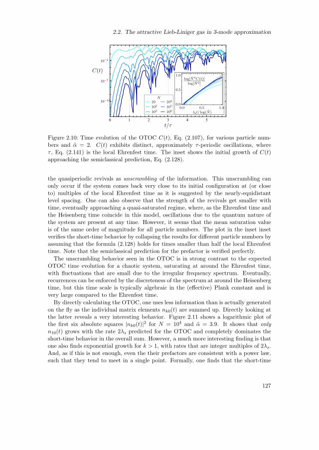
2.2. The attractive Lieb-Liniger gas in 3-mode approximation
Figure 2.10: Time evolution of the OTOC C(t), Eq. (2.107), for various particle num-bers and α = 2. C(t) exhibits distinct, approximately τ -periodic oscillations, whereτ , Eq. (2.141) is the local Ehrenfest time. The inset shows the initial growth of C(t)approaching the semiclassical prediction, Eq. (2.128).
the quasiperiodic revivals as unscrambling of the information. This unscrambling canonly occur if the system comes back very close to its initial configuration at (or closeto) multiples of the local Ehrenfest time as it is suggested by the nearly-equidistantlevel spacing. One can also observe that the strength of the revivals get smaller withtime, eventually approaching a quasi-saturated regime, where, as the Ehrenfest time andthe Heisenberg time coincide in this model, oscillations due to the quantum nature ofthe system are present at any time. However, it seems that the mean saturation valueis of the same order of magnitude for all particle numbers. The plot in the inset insetverifies the short-time behavior by collapsing the results for different particle numbers byassuming that the formula (2.128) holds for times smaller than half the local Ehrenfesttime. Note that the semiclassical prediction for the prefactor is verified perfectly.
The unscrambling behavior seen in the OTOC is in strong contrast to the expectedOTOC time evolution for a chaotic system, saturating at around the Ehrenfest time,with fluctuations that are small due to the irregular frequency spectrum. Eventually,recurrences can be enforced by the discreteness of the spectrum at around the Heisenbergtime, but this time scale is typically algebraic in the (effective) Plank constant and isvery large compared to the Ehrenfest time.
By directly calculating the OTOC, one uses less information than is actually generatedon the fly as the individual matrix elements nk0(t) are summed up. Directly looking atthe latter reveals a very interesting behavior. Figure 2.11 shows a logarithmic plot ofthe first six absolute squares |nk0(t)|2 for N = 104 and α = 3.9. It shows that only
n10(t) grows with the rate 2λs predicted for the OTOC and completely dominates theshort-time behavior in the overall sum. However, a much more interesting finding is thatone also finds exponential growth for k > 1, with rates that are integer multiples of 2λs.And, as if this is not enough, even the their prefactors are consistent with a power law,such that they tend to meet in a single point. Formally, one finds that the short-time
127

2. A semiclassical treatment of quantum critical phenomena
Figure 2.11: Left: Short-time behavior of the squared matrix elements |n0k(t)|2,Eq. (2.133), for N = 104 and α = 3.9 and for 1 ≤ k ≤ 6 (dots connected by solidlines) on a logarithmic scale. The dashed lines are given by N−2(α/λs)
4e2kλst, showingthat the matrix elements n0k(t) grow with a rate proportional to k. Right: Collapse ofthe n0k(t) for 1 ≤ k ≤ 8 using Eq. (2.143). The finite constant values at t = 0 for k ≥ 5(and beyond) are due to the numerical precision (∼ 10−16) of the matrix elements n0k(t)and indicate that the respective values are effectively zero there.
behavior of the matrix elements of the number operator n is very well described by
(4
N
)2
|nk0(t)|2 =
[(4
N
)2
|n10(t)|2]k
, (2.142)
such that they are not independent for short times. The last equation can be rewrittenin in the scaling form
[(4
N
)2
|nk0(t)|2] 1
k
=
(4
N
)2
|n10(t)|2 ∼ 1
N2
(α
λs
)4
e2λst, (2.143)
such that only the left hand side of the equation depends on k. The last scaling in(2.143) originates from the dominance of the k = 1 term for short times t . logN/λsand the short-time prediction for the OTOC, Eq. (2.128), together with the expansionof C(t) into the functions n0k(t). Thus, a more accurate short-time approximation ofthe OTOC (2.107) is given by
C(t) ≈ 1
N2
kcut∑
k=1
k2[
4
N|n01(t)|
]2k
≈kcut∑
k=1
k2
[(α
Nλs
)4
e2λst
]k
, (2.144)
where a cutoff kcut ≤ ⌊N/2⌋ was introduced that controls the “order” of approximation.The second approximation is only valid for some intermediate times, where the expo-nential approximation is justified. So, in this respect, the semiclassical short-time result(2.128) is just the first order approximation with kcut = 1 of an expansion into powersof exponential functions.
128
2.2. The attractive Lieb-Liniger gas in 3-mode approximation
Unfortunately, a theoretical explanation of this behavior has not been found yet.However, there are some hints that might help solving this problem. The reader mighthave noticed the large value of the interaction used in Fig. 2.11. One reason for this valueis to demonstrate that also the semiclassical prediction for the prefactor (α/λs)
4 ≈ 1.72in the equations is accurate. This could be better demonstrated at couplings close toα = 1, where this prefactor diverges. However, the universal behavior breaks down (atleast for N ≤ 104) when approaching this point (not shown). As this is the point wherethe two hyperbolic fixed points in the classical phase space come close to each other, anylocal description would have to take into account both fixed points. Conversely, the factthat the scaling (2.143) is valid for larger couplings, where the hyperbolic fixed pointsare well separated, could hint at a general feature of (isolated) hyperbolic fixed points.
The form of the short-time behavior of C(t) as a power series in eλst strongly resemblesthe Ansatz
F (t) = 〈χi(t)ρ14χj(0)ρ
14χi(t)ρ
14χj(0)ρ
14 〉 ≈ C0 + C1
eλt
N+ C2
(eλt
N
)2
+ . . . (2.145)
for the (regularized) thermal OTOC of Majorana operators χk in a (quenched) disorderaverage in the Sachdev-Ye-Kitaev model [174], that is motivated from a diagrammaticapproach that includes summing up certain classes of diagrams [208]. A closer analysis ofthe applicability of the approach to the model at hand could shed light on the mechanismleading to the observed behavior of the matrix elements n0k.
2.2.5. Perturbation with external potential
We have seen in the last subsection, that an interaction quench of the noninteractingcondensate leads to a quasi-periodic behavior of the out-of-time-ordered correlator thatcan be interpreted as successive scrambling and unscrambling of the information aboutthe initial configuration of the system. However, as the retrieval of the information onthe initial state is due to the dynamics close to a separatrix, one should ask the questionabout the robustness of the phenomenon against integrability breaking. In the classicalmean-field description one should expect that a small external perturbation of the systemshould manifest itself dominantly in the vicinity of the separatrix [42]. To be morespecific, if a trajectory comes close to a hyperbolic fixed points, the classical forces in theequations of motion get arbitrarily small, while the dynamics slow down exponentially,such that a small perturbation can have a large effect, leading to a stochastic layeraround the separatrix. On the other hand, a hidden renormalization group, that existsaround the (perturbed) hyperbolic fixed points [209], suggests that the local Ehrenfesttime τ , Eq. (2.67) might still play an important role, as it has exactly the analytic formof the required time renormalization.
The simplest way to get a nonintegrable extension of the 3-mode model consideredhere is obtained by breaking the conservation of the momentum K, Eq. (2.43). This canbe done by adding the perturbation
γV =γ
2
[
a†0(a1 + a−1) + (a†1 + a†−1)a0
]
(2.146)
129
2. A semiclassical treatment of quantum critical phenomena
to the Hamiltonian (2.42). It corresponds to an external potential of the form cos(θ) onthe ring in three-mode approximation. This perturbation has also been used to studythe finite-size effects on the collapse of the wave function [194], as for finite particlenumbers, the lowest energy eigenstates of the different momentum sectors have a finitegap with the unperturbed ground state, such that a finite perturbation is needed for alocalization of the state. If this finite critical perturbation value γc ∼ N−2 is exceeded, aGaussian momentum distribution is assumed, centered around the unperturbed groundstate with K = 0. However, for the excited state quantum phase transition, the effectof such a perturbation has not been investigated in detail, and it is not clear, how thedynamics after an interaction quench as considered above are affected. One possiblescenario is that the number of states that have a finite overlap with the noninteractingground state is strongly increased by the additional degree of freedom and the extensionof the quantum mechanical eigenstates along the stochastic layer in classical phase space.However, for finite perturbations, there should also be a regime, where the effect of theperturbation can be included via a perturbative expansion.
In the following, only a few results are presented that were obtained in a Bachelorproject by Dominik Hahn under supervision of the author of this thesis. In the classicalanalysis, the perturbation leads to an additional term in the scaled Hamiltonian (2.48),
∆ωγ(ϕ, z, ϕl, l) = γ
√z
2
[√1 − z + l cos(ϕ− ϕl) +
√1 − z − l cos(ϕ+ ϕl)
]
, (2.147)
such that the conjugate angle ϕl to l = Kcl/N is not cyclic anymore and the momentuml is not conserved. To investigate the classical dynamics one can make use of Poincaresections, i.e., by plotting only the (directed) intersections of the classical trajectorieswith a manifold of codimension one in phase-space (that is not parallel to the flow) [42].There are different choices for the surface, with the most common one being the planedefined by the cyclic angles from the unperturbed model that corresponds to the brokensymmetry in the perturbed model, usually guaranteeing (point-like) intersections in theunperturbed case. This would suggest that one should take the plane defined by ϕl = ϕl,0
and find all the points on a trajectory where the angle ϕl crosses this plane in the samedirection. However, this choice is not very good in the case at hand, as the angle ϕl isstationary in the unperturbed case for l = 0, as can be seen from the equation of motionfor ϕl in the unperturbed case
ϕl =∂ω
∂l=α
2
l cos 2ϕ√
(1 − z)2 − l2l→0−→ 0. (2.148)
For this reason, a different choice was made that is also better suited for comparisonwith the unperturbed case. By choosing the surface l = 0 for the Poincare map theunperturbed case is degenerate, as the trajectory does not leave this plane. However,any finite perturbation γ renders the intersections point-like due to ∆ωγ and is thussuited for the analysis. Figure 2.12 shows an overlay of many Poincare maps for differentenergies and for α = 1.9 and γ = 0.01. The reason for showing many different energiesis that the available regions in the surface of section with constant energy are small for
130

2.2. The attractive Lieb-Liniger gas in 3-mode approximation
Figure 2.12: Overlay of different Poincare surfaces of section. Different colors correspondto different energies. The initial values are l = 0 and random initial values in z, ϕ andϕl. As the random initial conditions did not hit the chaotic region, more random initialvalues were used in a ǫ = 0.1 window around the right fixed point, two of them beingshown in the plot.
γ ≪ 1 and become one-dimensional for γ → 0, reproducing the integrable case. This isthe drawback of using the unconventional surface of section l = 0. One can clearly see,that the perturbation is so small that most of the invariant tori are preserved. However,in the region around the separatrix of the unperturbed model, one can see a small chaoticlayer, as expected. This should manifest itself in the OTOC that is very sensitive to thisregion.
The OTOC has been calculated for various values of the perturbation γ and for N =100 and α = 1.8. A comparison is shown in Fig. 2.13. It shows that the oscillationsof the OTOC are very sensitive to the perturbation and get damped strongly for allthe values of γ shown in the plot. One has to stress, however, that the oscillationsseen in the nonperturbative result in Fig. 2.13 are not directly associated with the localEhrenfest time τ , Eq. (2.67), as the number of particles is not large enough to clearlysee its signatures, c.f., Fig. 2.10. Although the perturbation is varied over one order ofmagnitude, the mean value of the OTOC for later times seems to be rather insensitiveto the strength of the perturbation for the times shown in the plot. The inset showsthe short-time behavior of the ratio between the perturbed and unperturbed results forthe same values of γ, indicating that the perturbation leads to faster initial scrambling,reflected in a larger growth rate. However, the latter is still dominated by the classical(in)stability exponent λs ≈ 1.9 of the hyperbolic fixed points of the unperturbed system.This can be seen from the right part of Fig. 2.13, that shows the fitted difference ∆λ inthe growth rate from the ansatz
Cγ(t) ≈ C0(t)e2∆λt ∝ e2(λs+∆λ)t, (2.149)
showing that it is one order of magnitude smaller than λs. For the fits, a window
131

2. A semiclassical treatment of quantum critical phenomena
10 20 30 40 50
1.×10-4
5.×10-4
0.001
0.005
0
5.×10-5
0 2 4
1
2
4
0.00 0.05 0.10 0.150.0
0.1
0.2
0.3
0.4
Figure 2.13: Left: Out-of-time ordered correlator in the perturbed model for N = 100,α = 1.9 and various values of the perturbation γ (data of Dominik Hahn is used). Forlarger values of the perturbation, the oscillations of the OTOC are damped, but themagnitude of γ does not have a large effect on the saturation value for the times shown.The inset shows the short-time behavior of the ratio of perturbed and unperturbedOTOC, showing an additional increase due to the perturbation. Right: Comparison ofthe fitted growth rate with the classical Lyapunov exponent.
around the inflection points of the ratio Cγ(t)/C0(t) has been used. The ansatz (2.149)is motivated from the observation that, although the dynamics is not regular in thestochastic layer that emerges from the separatrix, it is still the dominant feature in thel = 0 surface, dividing two regular regions of phase space from each other. Classicallyevolving an ensemble of trajectories, characterized by a phase-space distribution, closeto this region, one can expect that the distribution eventually fills a three-dimensionalregion of phase space only constrained by the energy conservation and bounded bythe regular regions. But this can happen on very different time scales in the differentdirections, i.e., the divergence of two nearby trajectories due to the perturbation couldbe much smaller than the divergence due to the instability along the former fixed points.This should then manifest itself in a separation of scales in the OTOC, leading to twoindependent contributions to the initial scrambling rate.
This picture is strongly supported by the fact that the additional instability seems tocoincide very well with the (maximal) classical Lyapunov exponent λL (see Fig. 2.13)found from a long-time average over the divergence rate of two neighboring trajectoriesinitialized at z = 1/N and l = 0 (and maximizing with respect to the initial conditionsin ϕ, ϕl). The error bars come from a very slow convergence of the Lyapunov exponentdue to the strong influence of the instability around the hyperbolic fixed points. Ifthis apparent separation of scales persists also for larger particle numbers N , one mightexpect to see signatures of the unscrambling mechanism given by the local Ehrenfesttime τ for N → ∞, that should manifest itself in a significant decrease of the OTOC att ∼ τ . Unfortunately, the necessary numerical simulations have not been performed yetand are left for future analysis.
132
2.3. The attractive Lieb-Liniger gas in 5-mode approximation
2.3. The attractive Lieb-Liniger gas in 5-mode approximation
Up to this point, we have seen that the presence of a separatrix in the mean-field pictureof the Lieb-Liniger model in three-mode approximation gives rise to an excited statequantum phase transition that leads to an emergent universal time scale for processesthat dominantly involve the states in its vicinity. This time scale plays an importantrole in the post-quench time evolution, when the system is prepared as a noninteractingcondensate state and is then quenched to finite couplings above the mean-field criticalinteraction. The reason for this was found in the fact that the initial state did onlyoverlap with a few states around the classical separatrix energy, such that the dynamicsis dominated by the classical hyperbolic fixed points. However, all of the analysis hasbeen performed in the context of integrable systems, where the classical dynamics isconstrained to Lagrangian surfaces, which is also reflected the quantum dynamics. Al-though the influence of a perturbation has been studied very briefly, adding an externalpotential with a finite strength actually changes the system drastically: The quantumphase transition in the attractive Lieb-Liniger gas breaks the translational symmetry.Destroying this symmetry would lead to a localization of the eigenstates already withoutinteraction. As the (excited state) quantum phase transition is an essential ingredientfor the emergence of the universal quench dynamics found in the previous sections, oneshould find a nonintegrable extension that is critical.
The three-mode approximation is the simplest nontrivial approach to uncover thephysics of the quantum phase transition of the continuum model. As one should getbetter approximations by including more modes, one should also expect these refinedmodels to show critical behavior. Therefore, this section is dedicated to the analysis ofthe extension of the model by increasing the momentum cutoff in the field operators,Eq. (2.41), to kmax = 2, leading to a total of five modes that have to be included in theHamiltonian (2.42). As the conservation of the total particle number and momentum,Eq. (2.43), is robust under the truncation, one can still restrict the quantum and (classi-cal) mean-field analysis to fixed particle number and momentum, but the two additionaldegrees of freedom render the quantum and classical dynamics much more difficult. Infact, it is long known that, although the full model is quantum integrable, the cutoffsintroduce signatures of chaotic behavior in the nonlinear Schrodinger equation [210],i.e., the mean field equation of the model. This also manifests itself in level repulsionin the quantum-mechanical spectrum that can eventually lead to Wigner-Dyson levelstatistics in some parts of the spectrum [211]. It should be clear that these numerically-induced signatures of chaotic behavior are not the subject of interest here, as they haveno physical meaning. Obviously, the five-mode approximation should not be used for aquantitative analysis of the attractive Lieb-Liniger model whenever the variation of thecutoff introduces changes in the predictions. Therefore, as in the three-mode approxima-tion, the analysis of the five-mode model performed here aims at a better understandingof quantum phase transitions in a more general context, as an example of a quantumphase transition in a model that is not completely integrable in the mean field limit.
133

2. A semiclassical treatment of quantum critical phenomena
2.3.1. Classical phase space analysis
As discussed in subsection 2.1.2 of the introduction of this chapter, the mean-field equa-tions can be found as the classical equations of motion defined by the Hamiltonianfunction that is obtained by taking the classical limit of the quantum Hamiltonian. Forthis, one should replace the quantum operators by classical variables. However, to keeptrack of O(N−1) corrections one should first bring all the operator products in sym-metric order. This yields the Wigner phase space representation of the operator(s) (orWigner symbol), and the classical N → ∞ limit can be studied in a controlled way.The corrections should not have an influence on the classical dynamics, as the classicalequations of motion should be independent on the (effective) Planck constant, but theyplay an important role in the quantization of the classical system. Although this willnot be done for the five-mode model, the corrections from symmetrization are includedhere for completeness.
Symmetrizing products of creation and annihilation operators can become a very cum-bersome task when the number of operators grow. Already at the stage of a product offour bosonic operators, as needed to describe interactions, the direct calculation becomesquite lengthy and should be avoided. Fortunately, one can formulate a variant of a Wicktheorem to calculate symmetrized products [212]. The statement is as follows: For nbosonic operators A1, . . . , An, the symmetrization of their product is defined as
A1 · · · An
s=
1
n!
∑
P∈Sn
AP (1) · · · AP (n), (2.150)
where Sn is the symmetric group. Defining the contraction
A•i A
•j = AiAj − AiAjs =
1
2[Ai, Aj ], (2.151)
where [·, ·] is the commutator, one can define the sum of k-fold contractions of a productof operators as Ck(A1A2 · · · An). For example for k = 2, n = 4 one obtains three fullcontractions,
C2(A1A2A3A4) = A•1A
•2A
••3 A
••4 + A•
1A••2 A
•3A
••4 + A•
1A••2 A
••3 A
•4, (2.152)
where the double bullet is only used to distinguish the two contractions. With thesedefinitions the following theorem holds:
A1A2 · · · An =
⌊n/2⌋∑
k=0
Ck(A1A2 · · · An)
s, (2.153)
i.e., the product can be symmetrized in one step by summing over all possible (multiple)contractions.
134

2.3. The attractive Lieb-Liniger gas in 5-mode approximation
Using this Wick theorem on the Hamiltonian (2.42) with the usual commutation re-lations yields
H =∑
k
k2
a†kak
s− α
4
∑
k,l,m,n
δk+l,m+n
a†ka†l aman
s
+α
2
∑
k,l
(
a†kak
s− 1
4
)
−∑
k
k2
2. (2.154)
The second line contains the corrections due to the symmetric ordering of the operatorsand requires regularization if the cutoff is removed as is often the case in continuumsystems. Using the cutoff kmax = 2 and replacing the symmetrically ordered operatorsby products of (complex) classical variables, c.f., Eq. (2.45), one obtains the classicalHamiltonian function of the five-mode approximation as
H(cl)5 =
2∑
k=−2
(
k2 +5α
2
)
φ∗kφk −α
4
2∑
k,l,m,n=−2
δk+l,m+nφ∗kφ
∗l φmφn − 25α
8− 5. (2.155)
with the variables φk =√nke−iθk . The operators for the particle number and the
momentum can be treated in the same way by symmetrizing them and then replacingthe operators by complex numbers. However, as in the three-mode model, it is moreconvenient to define the classical constants of motion without the quantum correctionsas
N =2∑
k=−2
nk, K =2∑
k−2
knk. (2.156)
One can now proceed by eliminating the constants of motion with the linear pointtransformation
nN2K2
N
K
=
0 0 1 0 01/2 0 0 0 1/2−1/2 0 0 0 1/2
1 1 1 1 1−2 −1 0 1 2
︸ ︷︷ ︸
A
n−2
n−1
n0n1n2
, (2.157)
θ = ATϕ, (2.158)
where A was chosen such that the Jacobian is one and the angles ϕ can be chosen inan interval of length 2π. Note that the transformation is canonical, i.e., the angles ϕare the conjugate angles to the new variables. Due to the conservation of N and K,
their conjugate angles drop out from H(cl)5 . The explicit inversion of the transformation
(2.157) then yields
n0 = n, n±2 = N2 ±K2, n±1 =N − n− 2N2
2± K − 4K2
2. (2.159)
135
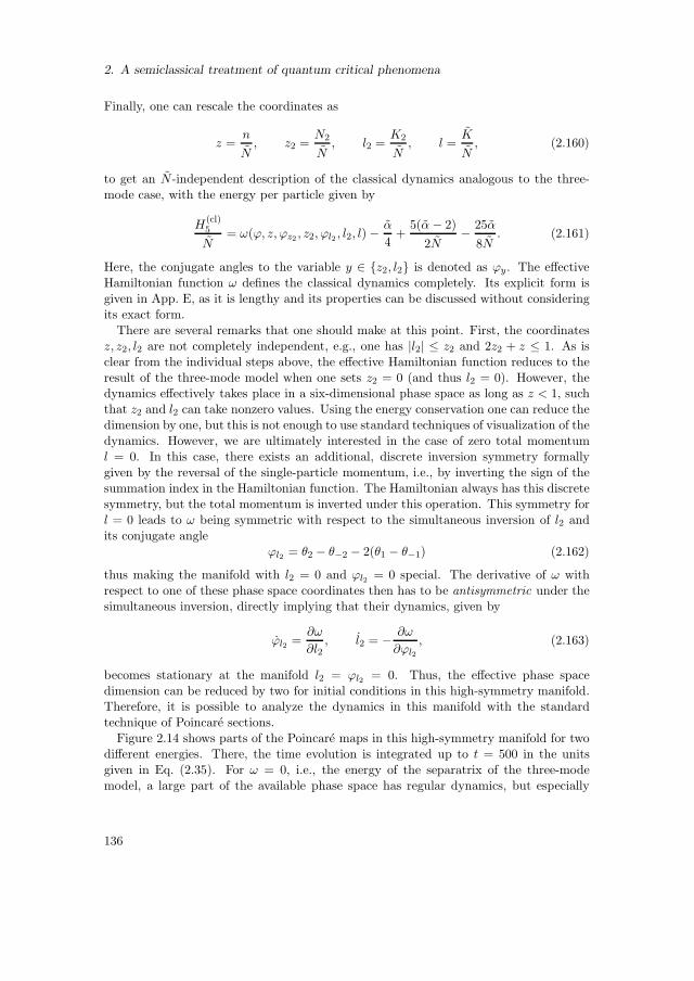
2. A semiclassical treatment of quantum critical phenomena
Finally, one can rescale the coordinates as
z =n
N, z2 =
N2
N, l2 =
K2
N, l =
K
N, (2.160)
to get an N-independent description of the classical dynamics analogous to the three-mode case, with the energy per particle given by
H(cl)5
N= ω(ϕ, z, ϕz2 , z2, ϕl2 , l2, l) −
α
4+
5(α − 2)
2N− 25α
8N. (2.161)
Here, the conjugate angles to the variable y ∈ z2, l2 is denoted as ϕy. The effectiveHamiltonian function ω defines the classical dynamics completely. Its explicit form isgiven in App. E, as it is lengthy and its properties can be discussed without consideringits exact form.
There are several remarks that one should make at this point. First, the coordinatesz, z2, l2 are not completely independent, e.g., one has |l2| ≤ z2 and 2z2 + z ≤ 1. As isclear from the individual steps above, the effective Hamiltonian function reduces to theresult of the three-mode model when one sets z2 = 0 (and thus l2 = 0). However, thedynamics effectively takes place in a six-dimensional phase space as long as z < 1, suchthat z2 and l2 can take nonzero values. Using the energy conservation one can reduce thedimension by one, but this is not enough to use standard techniques of visualization of thedynamics. However, we are ultimately interested in the case of zero total momentuml = 0. In this case, there exists an additional, discrete inversion symmetry formallygiven by the reversal of the single-particle momentum, i.e., by inverting the sign of thesummation index in the Hamiltonian function. The Hamiltonian always has this discretesymmetry, but the total momentum is inverted under this operation. This symmetry forl = 0 leads to ω being symmetric with respect to the simultaneous inversion of l2 andits conjugate angle
ϕl2 = θ2 − θ−2 − 2(θ1 − θ−1) (2.162)
thus making the manifold with l2 = 0 and ϕl2 = 0 special. The derivative of ω withrespect to one of these phase space coordinates then has to be antisymmetric under thesimultaneous inversion, directly implying that their dynamics, given by
ϕl2 =∂ω
∂l2, l2 = − ∂ω
∂ϕl2
, (2.163)
becomes stationary at the manifold l2 = ϕl2 = 0. Thus, the effective phase spacedimension can be reduced by two for initial conditions in this high-symmetry manifold.Therefore, it is possible to analyze the dynamics in this manifold with the standardtechnique of Poincare sections.
Figure 2.14 shows parts of the Poincare maps in this high-symmetry manifold for twodifferent energies. There, the time evolution is integrated up to t = 500 in the unitsgiven in Eq. (2.35). For ω = 0, i.e., the energy of the separatrix of the three-modemodel, a large part of the available phase space has regular dynamics, but especially
136

2.3. The attractive Lieb-Liniger gas in 5-mode approximation
Figure 2.14: Poincare sections in the high-symmetry manifold with l2 = ϕl2 = 0 for twodifferent energies and α = 1.9. The section is taken at the points ϕz2 = 0 (mod 4π) withϕz2 > 0 and different colors correspond to different trajectories. For ω = 0 the dynamicsin the symmetry manifold has large regular structures that resemble the typical KAMscenario of broken rational tori [42], but the dynamics close to the hyperbolic fixed pointof the three mode model (red dot) is chaotic. For ω = 0.2 a large chaotic layer exists,verifying the non-integrability of the model. The apparently missing parts of the leftplot are probably due to the detection algorithm, but this has not been checked.
when approaching the hyperbolic fixed point of the 3-mode model (red dot in the upperright corner), one finds a chaotic layer. One should note that the plots show only asmall part of the Poincare section. The motion in ϕ is now 2π periodic instead of π-periodic, as would be the case for z2 = 0 (three-mode model). Also, one importantdetail has been omitted so far: Instead of fixing the angle ϕl2 to zero, one finds the samestationary behavior for ϕ = 2πn with n being any integer. But for odd n this is not thesame physical point, as shifting ϕl2 by 2π shifts the original angles θ±2 only by π. Thiscan also be seen in the Hamiltonian function (see App. E), where setting ϕl2 = 0 andϕl2 = 2π lead to different Hamiltonian functions. However, shifting both ϕl2 and ϕz2
by 2π yields the same physical point, c.f., Eq. (2.158), such that ϕl2 = 0 and ϕl2 = 2πdescribe the same manifold, with ϕz2 ranging over an interval of 4π. Therefore, fixingϕl2 = 0 or ϕl2 = 2π in the calculation only leads to solutions that are shifted by 2π inϕz2 . To demonstrate that the π-periodicity of the three-mode model is lost, Fig. 2.15shows the full Poincare section for ω = 0.2 and α = 1.9, i.e., the same values as in theright plot of Fig. 2.14.
Concluding, we have found that the classical dynamics in the special manifold thatis invariant under the mirror symmetry operation, is mixed, i.e., it contains regularand chaotic regions. Therefore, one can exclude that the five-mode model is classicallyintegrable and it is expected that the additional degree of freedom ϕl2 will render therest of the phase space such that there is no further (global) constant of motion forα 6= 0 and the dynamics will take place in the six-dimensional phase space in general10.When the coupling approaches the mean-field critical value of the interaction α = 1,
10However, one can get arbitrarily close to integrability in the limit α → 0.
137
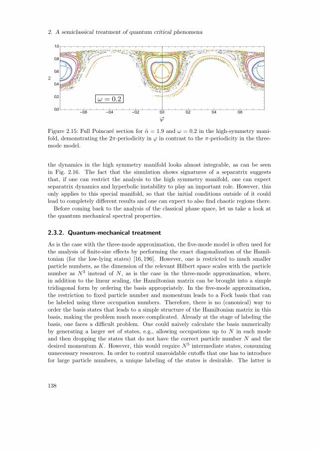
2. A semiclassical treatment of quantum critical phenomena
Figure 2.15: Full Poincare section for α = 1.9 and ω = 0.2 in the high-symmetry mani-fold, demonstrating the 2π-periodicity in ϕ in contrast to the π-periodicity in the three-mode model.
the dynamics in the high symmetry manifold looks almost integrable, as can be seenin Fig. 2.16. The fact that the simulation shows signatures of a separatrix suggeststhat, if one can restrict the analysis to the high symmetry manifold, one can expectseparatrix dynamics and hyperbolic instability to play an important role. However, thisonly applies to this special manifold, so that the initial conditions outside of it couldlead to completely different results and one can expect to also find chaotic regions there.
Before coming back to the analysis of the classical phase space, let us take a look atthe quantum mechanical spectral properties.
2.3.2. Quantum-mechanical treatment
As is the case with the three-mode approximation, the five-mode model is often used forthe analysis of finite-size effects by performing the exact diagonalization of the Hamil-tonian (for the low-lying states) [16, 196]. However, one is restricted to much smallerparticle numbers, as the dimension of the relevant Hilbert space scales with the particlenumber as N3 instead of N , as is the case in the three-mode approximation, where,in addition to the linear scaling, the Hamiltonian matrix can be brought into a simpletridiagonal form by ordering the basis appropriately. In the five-mode approximation,the restriction to fixed particle number and momentum leads to a Fock basis that canbe labeled using three occupation numbers. Therefore, there is no (canonical) way toorder the basis states that leads to a simple structure of the Hamiltonian matrix in thisbasis, making the problem much more complicated. Already at the stage of labeling thebasis, one faces a difficult problem. One could naively calculate the basis numericallyby generating a larger set of states, e.g., allowing occupations up to N in each modeand then dropping the states that do not have the correct particle number N and thedesired momentum K. However, this would require N5 intermediate states, consumingunnecessary resources. In order to control unavoidable cutoffs that one has to introducefor large particle numbers, a unique labeling of the states is desirable. The latter is
138
2.3. The attractive Lieb-Liniger gas in 5-mode approximation
Figure 2.16: Poincare section for α = 1.05 and ω = 0.01. The dynamics looks regularand one can clearly see evidence of a separatrix separating two different regions in phasespace. The Trajectories are sampled more frequently when they approach one of thehyperbolic points, indicating a slowdown of the (ϕ, z)-dynamics.
a tedious task, but it can be performed to full generality and is given in Appendix E.One then finds that the size of the basis in the K = 0 sector scales roughly as N3/36.Therefore, the bottleneck for the exact diagonalization is of the order of hundreds ofparticles. For larger particle numbers, one has to find schemes for approximations.
Figure 2.17 shows the low-lying spectrum for K = 0 and N = 30 (left) and N = 250(right). One immediately sees that one obtains a much richer spectrum as comparedwith the three-mode model, that only produce a series similar to the lowest states seenin the right plot (N = 250), that can be adiabatically connected to the lowest levels ofthe rays starting at α = 0. On first glance, one might think that the additional levels cancross these three-mode-type level series, which would hint at an additional symmetry.However, a closer analysis of these level “crossings” reveals a small, but finite levelrepulsion. This has been checked for several particle numbers and many different states,revealing avoided crossings in all cases (although some of the gaps turned out to beof the order 10−8 and below, however still well above machine precision). Althoughthe gaps are very small for the low-lying spectrum, the higher excited states have amore pronounced level repulsion and one can expect the level statistics to be far fromPoissonian, the latter characterizing generic integrable systems. In fact, it has beenshown that even in the repulsive Lieb-Liniger gas, the level statistics agree remarkablywell with the Wigner-Dyson distribution in the middle of the spectrum due to the cutoff,i.e., the levels are essentially distributed according to random matrix theory [211]. Thisagrees very well with the classical analysis of the mirror-symmetric manifold, where thechaotic regions grow when the energy is increased. However, in the low-energy regime,the spectrum looks rather regular.
139

2. A semiclassical treatment of quantum critical phenomena
Figure 2.17: Low-lyings spectrum of the five-mode model for K = 0. Left: N = 30particles. A new type of states exists, that was absent from in the three-mode model.The states seem to cross, hinting at a symmetry, however a closer analysis reveals avoidedcrossings. Right: N = 250 particles. The spectrum gets more complicated at higherexcitations but seems to have a clear structure. Certain levels get quasi-degenerate atα > 1.
2.3.3. Separation of scales and Born-Oppenheimer-type approximations
The fact that the classical dynamics is rather regular around the separatrix energyω = 0 even for very strong interactions, c.f., Fig. 2.14, with only a small stochasticlayer that seems to emerge from the separatrix of the three-mode model, suggests thatthe dynamics in the coordinates (ϕ, z) will be strongly affected by a (coarse-grained)hyperbolic dynamics. This means that the dynamics in (ϕ, z) is expected to slow downdue to this hyperbolicity, rendering the dynamics in the other coordinates much faster (ifthey do not share the same hyperbolic behavior). This motivates a Born-Oppenheimertype ansatz for separation of scales between the slow hyperbolic dynamics associated tothe separatrix and the fast dynamics in the other directions.
This can be viewed in a more general context for other systems that allow for amean-field description in terms of classical dynamics. A quantum phase transition is notexpected to take place in a completely chaotic, and therefore structureless phase space.One can, at least, expect an regular “skeleton” that can separate different regions inphase space. A phase transition should then be associated with changes in these regularstructures, i.e., the state has to be associated to different regions of phase space on eitherside of the transition in order to have different quantum mechanical properties. Thiscould be the transition from a regular to a chaotic region, or, as is the case in the three-mode model and will be argued to hold also for the five-mode model, is the transitionbetween two regular regions in phase space that are separated by a (weakly disturbed)separatrix. Even if a separation of scales is possible, the hardest part is to identify thefast and slow degrees of freedom. In the standard application of Born-Oppenheimerseparation of scales in molecules or solids, the very different masses of electrons andnuclei, together with the standard form of the Hamiltonian as a quantized mechanicalproblem with the position operators appearing only in the potential, render the choices
140
2.3. The attractive Lieb-Liniger gas in 5-mode approximation
rather obvious. Moreover, the quantum mechanical solutions of the (fast) electronicproblem is only parametrized by the positions of the nuclei, but not their momentum.
However, the classical dynamics obtained in mean-field descriptions can have a verydifferent structure, often with potentials that depend on both conjugate classical vari-ables. Still, the situation can be special for critical systems. If one of the classical phasespace variables can be used as an order parameter, it has to behave differently on bothsides of the transition and, assuming that the transition is due to a separatrix, should besensitive to the exponential slowdown due to the hyperbolic dynamics at the transition.Therefore, the idea is to use the variable z, that can be used as an order parameterin the three-mode and the full model, as well as its conjugate angle as a slow degreeof freedom. This is expected to work well close to the ground state phase transitionat α ≈ α = 1. As was seen in Fig. 2.14 for α = 1.9, the separatrix is replaced by achaotic layer for strong coupling. However, for α = 0.05 the dynamics is more regular,and a clear signature of a separatrix can be found close to ω = 0. Another reason tochoose a value close to α = 1 is the numerical observation that the series of states thathave a counterpart in the three-mode model develop a bunching of energy levels at anenergy that lies below the other level series and are thus energetically separated, as itcan already be seen in Fig. 2.17 for N = 250.
Up to this point, classical arguments have been used to identify a slow degree offreedom. A quantum mechanical generalized Born-Oppenheimer type approach couldbe applied by using the framework of adiabatic perturbation theory [213, 214]. Here,however, the insights gained from the classical picture are used to simplify the quan-tum calculations. The essence of the idea used here is that the characteristic energyscale introduced by the fast dynamics is larger than the ones from the slow dynamics,which is perfectly consistent with the level bunching at excited state quantum phasetransitions, leading to a very small energy spacing. By assuming that the fast degreesof freedom, i.e., z2, l2 and the conjugate angles get quantized to a ground state energy
E(fast)0 (ϕ, z) depending on the values of the slow variables z, ϕ, one could, in principle,
derive an effective model for the slow variables for finite N (being the effective inversePlanck constant) by using the phase space representations of the states corresponding to
E(fast)0 (ϕ, z). However, if one is interested in the mean field limit N → ∞, the situation
is simpler, as the respective states localize at the energy minimum of the fast degrees of
freedom (for fixed ϕ, z) with the energy given by the classical minimum E(fast)min (ϕ, z). As
this energy minimum can only be obtained numerically, a further refinement for finiteparticle numbers, e.g., by a semiclassical quantization of the fast degrees of freedom in alocal approximation, can only be performed semi-analytically and has not been achievedyet. Still, already at the level of the effective mean-field description and using only the
energy minimum E(fast)min (ϕ, z), one can extract nontrivial information. Figure 2.18 shows
a phase space portrait of this effective description for α = 1.05 obtained from replac-ing the phase space coordinates z2, l2 and their conjugate angles by the position of theenergy minimum. The minimization has been obtained by noticing that ϕl2 = l2 = 0solves two of the stationary conditions for a minimum and then minimizing with respectto the coordinates ϕz2 , z2 for fixed (ϕ, z). This leads to a unique choice of (ϕz2 , z2) for
141
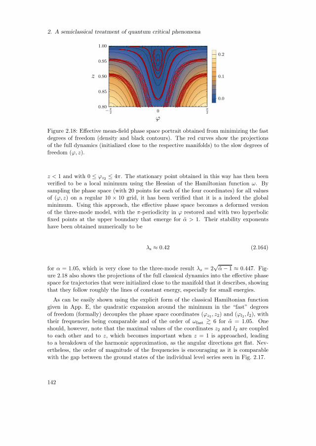
2. A semiclassical treatment of quantum critical phenomena
Figure 2.18: Effective mean-field phase space portrait obtained from minimizing the fastdegrees of freedom (density and black contours). The red curves show the projectionsof the full dynamics (initialized close to the respective manifolds) to the slow degrees offreedom (ϕ, z).
z < 1 and with 0 ≤ ϕz2 ≤ 4π. The stationary point obtained in this way has then beenverified to be a local minimum using the Hessian of the Hamiltonian function ω. Bysampling the phase space (with 20 points for each of the four coordinates) for all valuesof (ϕ, z) on a regular 10 × 10 grid, it has been verified that it is a indeed the globalminimum. Using this approach, the effective phase space becomes a deformed versionof the three-mode model, with the π-periodicity in ϕ restored and with two hyperbolicfixed points at the upper boundary that emerge for α > 1. Their stability exponentshave been obtained numerically to be
λs ≈ 0.42 (2.164)
for α = 1.05, which is very close to the three-mode result λs = 2√α− 1 ≈ 0.447. Fig-
ure 2.18 also shows the projections of the full classical dynamics into the effective phasespace for trajectories that were initialized close to the manifold that it describes, showingthat they follow roughly the lines of constant energy, especially for small energies.
As can be easily shown using the explicit form of the classical Hamiltonian functiongiven in App. E, the quadratic expansion around the minimum in the “fast” degreesof freedom (formally) decouples the phase space coordinates (ϕz2 , z2) and (ϕl2 , l2), withtheir frequencies being comparable and of the order of ωfast & 6 for α = 1.05. Oneshould, however, note that the maximal values of the coordinates z2 and l2 are coupledto each other and to z, which becomes important when z = 1 is approached, leadingto a breakdown of the harmonic approximation, as the angular directions get flat. Nev-ertheless, the order of magnitude of the frequencies is encouraging as it is comparablewith the gap between the ground states of the individual level series seen in Fig. 2.17.
142

2.3. The attractive Lieb-Liniger gas in 5-mode approximation
Numerical implementation
To implement the adiabatic separation on a quantum-mechanical level, simply replacingthe creation and annihilation operators corresponding to the zero mode by complexvariables leads to a U(1)-symmetry-broken effective description for the fast degrees offreedom with an infinite-dimensional Hilbert space, rendering this approach not suitablefor numerical diagonalization. Thus, a different approach has been taken here thatconsists of a pre-diagonalization of the projections of the Hamiltonian to subspaces ofthe Hilbert space H with a fixed mean condensate fraction z = n0/N . In particular, a“good” basis is found using the subspaces
Rk = H2k−1 ⊕H2k (2.165)
with k = 1, . . . , N/2 (and N even for simplicity), where
Hn = |ψ〉 ∈ H : a†0a0|ψ〉 = n|ψ〉 (2.166)
is the subspace with fixed particle number N , total momentum K = 0 and zero-modeoccupation n. This choice is motivated by the structure of the three-mode model, whereincrements of the occupations n0 are restricted to even numbers, and it is the minimalchoice that can capture the interplay between all the degrees of freedom. The latterfollows from the fact that fixing the occupation n0 exactly, projects out all the (off-diagonal) parts of the Hamiltonian that couple to this mode and thus misses the wholecomplexity of the problem. In the classical picture, this would correspond to dropping allterms that depend on the corresponding angle ϕ, completely decoupling the dynamics.So, combining two different occupations of the zero mode provides the minimal necessaryinformation about the phase ϕ.
The dimension of the space Rk scales as (N − 2k)2, such that the projections of theHamiltonian to Rk can be effectively diagonalized for large particle numbers, yielding
a k-dependent eigenbasis v(k)ν : ν = 0, 1, . . . (ordered by energy) that spans Rk. The
space span(v(k)ν : k = 0, 1 . . . ) may then be referred to as the ν-th band. An effectiveHamiltonian is found by restricting the full Hamiltonian to the space
Sζη =
ζ⊕
k=1
span(v(k)ν : ν ≤ η), (2.167)
where a cutoff 2ζ ≤ N in the condensate depletion has been introduced, as well as acutoff η controlling the number of excitations in the fast degrees of freedom taken intoaccount via inter-band coupling. It turns out that already for η = 0, where the effectiveHamiltonian has the same structure as for the 3-mode approximation, the low-lyingexcitation spectrum around the critical point α = 1 is well described. For the numerical
calculations of the vectors v(k)ν two further cutoffs
Σ2 = n2 + n−2 ≤ Σmax2 , ∆2 = |n2 − n−2| ≤ ∆max
2 (2.168)
143

2. A semiclassical treatment of quantum critical phenomena
were introduced, where n2, n−2 are the occupations of the ±2 single-particle momentummodes. The quantities Σ2 and ∆2 correspond directly to the classical variables z2 andl2, respectively.
For K = 0, the inversion symmetry of the system allows for a further reduction ofthe dimension by using the symmetric and antisymmetric states that cannot couple viathe parity-preserving Hamiltonian. For this, before diagonalizing the Rk-projections, aprojection to the symmetric subspace that contains both the interacting and noninter-
acting ground state has been performed, resulting in the vectors v(k)ν being only of this
symmetry class.
Characterization of the low-lying spectrum
As has been seen in Fig. 2.17, the different level series, or bands, can be identified byadiabatically relating them to the rays in the perturbative α≪ 1 regime. Although thenumerical scheme sketched above allows one to get to very large particle numbers, thecomputational effort is still very high, such that calculating an energy flow diagram, i.e.,the dependence of the spectrum with respect to the coupling, cannot be done for largeparticle numbers to high precision, as all calculations have to be repeated if the couplingα changes. Moreover, the adiabatic connection can only be made by coarse graining(i.e., “by eye”), as the actual energy levels do not cross. Therefore, and for the sake of adeeper physical understanding, it is desirable find a way to distinguish states in differentbands without knowing their functional dependence on the coupling α.
Unfortunately, due to the pre-diagonalization in the numerical scheme, the resultingeffective Hamiltonian and its eigenfunctions contain random sign factors, as the numer-
ically obtained vectors v(k)ν are only defined up to a phase or, restricting to real vectors,
up to its sign, that is randomly picked by the Arnoldi algorithm used for diagonalization.
The final eigenstates are thus useless for any further analysis, if the vectors v(k)ν are not
known, but keeping the latter quickly produces very large amounts of data that containfar too much information. However, one can perform the stepwise projections to thespaces Sζ
η for many operators simultaneously without significantly increasing the com-putational effort (as long as they are sparse in the Fock basis), imprinting the randomsigns also in these projected operators, that can then be used to analyze the propertiesof the final eigenstates.
The obvious choice is to calculate, together with the effective Hamiltonian, the pro-jected versions of the number operators. But only three of them are independent dueto the number and momentum conservation, and the restriction to inversion-symmetricstates reduces the number of independent number operators to two, e.g., n0 and n2. Agood choice of simple operators is given by
n0, N2 =n2 + n−2
2, K2
2 = (n2 − n2)2, (2.169)
as these operators are parity-symmetric, such that no information is lost due to thesymmetry projection. Note that these operators correspond to the variables z, z2 andl22 used in the classical analysis. For more generality, one might also want to include
144

2.3. The attractive Lieb-Liniger gas in 5-mode approximation
−25 −20 −15 −10 −5 0energy
0.00
0.05
0.10
0.15
0.20
0.25
0.30
mea
n_n2
0.05
0.10
0.15
0.20
0.25
0.30
0.35
mea
n_l2sq
0.1 0.2 0.3 0.4 0.5mean_n2
0.000
0.025
0.050
0.075
0.100
0.125
0.150
0.175
0.200
mea
n_l2sq
0.000001
0.000002
0.000003
0.000004
0.000005
0.000006
0.000007
var_n1
Figure 2.19: Left: Scatter plot of the energies and the the expectation values of N2 forthe first 100 energy levels and for N = 100, α = 1.1. The color represents the expectationvalues of K2
2 . Right: Scatter plot of the expectation values of N2 and K22 for the same
states with the variance of (n1 + n−1)2 as color code. The different scale of the latter is
due to rescaling with the particle number and is of no importance here.
products of the operators 2.169, but this has not been done, as the above operators haveturned out as a good choice to characterize the eigenstates already on the basis of theenergy eigenstate expectation values
meank(N2) = 〈ψk|N2|ψk〉 ,vark(K2) = 〈ψk|K2
2 |ψk〉 , (2.170)
vark(N1) = 〈ψk|(n1 + n−1)2|ψk〉 ,
where k is a label of the eigenstate. The last variance in Eq. (2.170) has been calculatedfrom the projected operators (2.169) using
n1 + n−1 = N − 2N2 − n0 (2.171)
and is thus not exact, but this has turned out to be irrelevant in the following.
Figure 2.19 shows scatter plots of the energy and the expectation values (2.170) forthe first 100 levels for N = 100 and α = 1.1. The left plot clearly shows that the stateshave very different mean occupations in the side modes, characterized by meank(N2),leading to distinct series in the scatter plot. However, the colors show that including thevariance in the side-mode imbalance, vark(K2), can distinguish states that lie on top ofeach other. This is clarified in the right plot, where the aforementioned quantities areplotted against each other, revealing distinct series that were lying on top of each otherin the left plot. As some of the series can overlap in the two-dimensional scatter plots,the variance vark(N1) can be used to lift this into three dimensions.
Using the cluster detection algorithm DBSCAN implemented in Python [215,216], thedifferent series have then be labeled automatically (cutting off noisy parts). The resultcan be seen in Fig. 2.20, where each series of states has been given a label. Note the twooutliers that have been characterized as noise. They correspond to hybrid states close
145

2. A semiclassical treatment of quantum critical phenomena
−28 −26 −24 −22 −20 −18 −16 −14energy
0.0
0.2
0.4
0.6
0.8
1.0
mean_n2
−1
0
1
2
3
4
5
band
s
Figure 2.20: Result of automatic state labeling using the cluster detection algorithmDBSCAN. The cluster detection works better if the particle number is increased. Right:Sketch of the harmonic oscillator spectrum analogy of the level series, with the gray-shaded area representing the band structure.
to an avoided crossing. The quality of the result needed some fine-tuning for N = 100,but for higher particle numbers, the cluster detection is quite reliable, allowing one todirectly select the states from a specific band.
One observation is that the states in the low-lying spectrum can be characterized bythree “good” quantum numbers (N2,K2,m). The first two can be used to label the bandand the excitation within each band is then labeled by m. To be specific, the quantumnumber N2 = 0, 1, 2, . . . labels the series of degenerate bands seen in the left part ofFig. 2.19 according to meank(N2), starting from the bottom. Then, for given N2, thequantum number K2 can be chosen as
L2 =
0, 2, . . . , N2 N2 even
1, 3, . . . , N2 N2 odd(2.172)
that are assigned to each of the degenerate bands with the same label N2 according tothe mean value of [vark(K2)]1/2 in each band. The index m then just labels the stateswithin each band (N2, L2).
The above characterization of the bands with two numbers (N2, L2) reminds of atwo-dimensional harmonic oscillator spectrum that is given by the sum of two quantumnumbers Eho = ~ω(k1 + k2 + 1) being highly degenerate. Instead of using k1, k2 onecan label the states by Nho
2 = k1 + k2 and Lho2 = k1 − k2. The energy then depends
only on N2, as is the case in the five-mode model, while the eigenstates will dependalso on L2. The analogy is further underlined by the following two observations: First,the energy of the lowest state [k = (N2, L2,m = 0)] of each band depends linearly onthe N2 ∼ meanN2,L2,0(N2) (see left part of Fig. 2.19) as is the case for the harmonicoscillator. Second, by rescaling the vertical axis in the right part of Fig. 2.19 by plottingthe square-root of L2 ∼ var(K2) will give a pattern very similar to the sketch in the rightpart of Fig. 2.20 that shows the pattern of quantum numbers in the two-dimensionalharmonic oscillator. Finally, by not distinguishing between positive and negative values
146

2.3. The attractive Lieb-Liniger gas in 5-mode approximation
of Lho2 one ends up exactly with the observed rules for the quantum numbers N2 and L2
of the fast degrees of freedom in the five-mode model.
Therefore, this section concludes with the claim that the fast degrees of freedomare basically two-dimensional harmonic oscillator states. Due to the mirror symmetrythat holds for K = 0, these states are combined to symmetric (and antisymmetric)superpositions that correspond to the superpositions of harmonic oscillator states withthe same |Lh0
2 | = |k1 − k2|. It is expected that including the antisymmetric states inthe analysis will fill up the gap of the apparently missing bands, then leading to anindexation of the bands similar to a two-dimensional harmonic oscillator using N2, theabsolute value |L2| and a symmetry index ±1 that can distinguish the states with L2 6= 0according to their mirror symmetry. The last point is supported by the observation thatthe energies of the antisymmetric states are almost degenerate with a set of levels of thesymmetric class (not shown).
2.3.4. Rigidity of (excited states) quantum phase transition
Now, being able to push the particle numbers in the five-mode model to much higher val-ues of the order of 104 particles, we are in the position to analyze the large-N asymptoticbehavior and answer the question of whether an excited state quantum phase transitionis expected to appear in the mean-field limit. The existence of the latter led to thedistinct local Ehrenfest time scale in the three-mode model and dominated the quenchdynamics of the noninteracting condensate there. The goal here is to show that the ex-cited state phase transition exists also in the five-mode model and that it also implies thelocal Ehrenfest time as the dominant time scale in the aforementioned quench scenarios.
As a major result, the individual sub-spectra have a regular level spacing as expectedfrom 1D systems, with a peak in the density of states at the energy of the separatrix of theeffective phase space. This is demonstrated in Fig. 2.21, where the inverse level spacingwithin the lowest sub-spectrum is shown and compared to the result from the three-mode model. Moreover, the noninteracting condensate overlaps dominantly with stateswithin this peak (gray shaded curve in Fig. 2.21), indicating that the quench dynamicsof this state is dominated by only a few states around an excited state quantum phasetransition with level spacings that can be expected to be asymptotically equidistant. Thisis because of the evident and remarkable similarity of the results from the three-modeand five-mode model, that allows to transfer the analytical results of the three-modemodel to the five-mode model in this special situation of the excited state quantumphase transition. One should note, however, that there are clearly differences in thetwo models, that can already be seen from Fig. 2.21. First, the inverse level spacingis enhanced by approximately 10% in the five-mode model. Second, and much moreimportant, one has more levels below the peak in the five-mode model and the groundstate of the three-mode model (not shown, as k ≥ 1 in the plot) is approximately at theenergy of the k = 9 excited state in the five-mode model.
The dominance of a local Ehrenfest time scale similar to the three-mode model case isdemonstrated in Fig. 2.22, where the quench dynamics after an interaction quench fromthe noninteracting condensate to a coupling of a = 1.05 is shown for different particle
147

2. A semiclassical treatment of quantum critical phenomena
Figure 2.21: Comparison of the inverse level spacing in the three-mode model (orange)and the first level series/band in the five-mode model for N = 5000, α = 1.05. The dotsrepresent the actual energy levels, and the solid lines are for better visibility (but canbe interpreted as the smooth density of states). Both models show the characteristiclogarithmic peak in the density of states. The yellow/gray shaded plot shows the squaredoverlaps (multiplied by 20) of the eigenstates |ψk〉 with energy Ek of the three-/five-modemodel with the noninteracting ground state.
Figure 2.22: Comparison of the quench dynamics of the entropy of the reduced one-body density matrix (top) and the OTOC (2.107) (bottom) in the five-mode (left) andthree-mode (right) model for α = 1.05 and different particle numbers. The constant C0
facilitates the comparison in the case of the five-mode model.
148

2.3. The attractive Lieb-Liniger gas in 5-mode approximation
Table 2.1: Cutoffs that were used in the numerical calculations.
N 100 500 1000 1500 5000 10000
ζ 40 100 200 300 1000 2000
∆max2 20 30 20 30 50 50
Σmax2 40 60 40 60 100 100
numbers. The top panel shows the time evolution of the von Neumann entropy
S(t) = −Tr ρ(t) log ρ(t) (2.173)
of the reduced one-body density matrix
ρij(t) = 〈Ψ(t)|a†i aj|Ψ(t)〉 , (2.174)
where |Ψ(t)〉 is the noninteracting condensate evolved for the time t in the interactingsystem. One can clearly see the emergence of the first revival at the local Ehrenfest timeτ , that has been estimated from the average level spacing around the separatrix, withthe number of states taken into account scaling like log(N). The latter is consistentwith the original derivation of the local Ehrenfest time in the three-mode model [189].Fitting the obtained values for τ to
τ =logN
λ+ c (2.175)
for the different particle numbers, where c accounts for O(1) corrections, one finds λ ≈0.21, being in excellent agreement with the stability exponent λs = 0.42, Eq. (2.164),found in the classical analysis of the effective phase space. Although the dynamics ofthe entropies look very similar, the additional modes in the five-mode approximationlead to higher absolute values. The three-mode result uses the finite-size-corrected localEhrenfest time (2.141). The lower panel of Fig. 2.22 shows the out-of-time-orderedcorrelator C(t), Eq. (2.107), for the five- and three-mode model, clearly showing thesignatures of unscrambling in both cases with very similar time dynamics. Althoughthe quantum revivals seem to be much weaker, the comparison with the OTOC in thethree-mode model shows that this is rather due to the choice of parameters leading to asmall separatrix. However, one can expect the revivals to become more pronounced forlarger particle numbers even in the OTOC, as can be seen for N = 50000 in the three-mode case that behaves very similar to the five mode model for the particle numbers upto N = 5000.
For the plots in Fig. 2.22, all cutoffs have been varied to check the convergence of theresults. The data presented here uses the cutoffs shown in table 2.1, where η = 80 for allthe values of N . The time evolution was approximated using the first 2000 eigenstatesof the effective Hamiltonian matrix for particle numbers N ≥ 500 (for N = 100 alleigenstates were used). The convergence of the results with respect to this approximationhas been checked, again, by varying the number of eigenstates.
149
2. A semiclassical treatment of quantum critical phenomena
At this point it is not clear whether the results obtained so far for the five-mode modelcan be extended to stronger couplings, where the stochastic layer around the separatrixcould lead to faster scrambling and weaker revivals.
150
2.4. Summary and concluding remarks
2.4. Summary and concluding remarks
In this chapter, a semiclassical approach to (quantum) phase transitions of the groundstate, but also excited states has been presented. After introducing the necessary tools,the attractive one-dimensional Bose gas in three mode approximation was studied bymeans of the semiclassical torus quantization of its integrable classical dynamics. It hasbeen shown that the ground and excited state quantum phase transitions have theirorigin in the emergence of a separatrix in the classical phase space. With this, a criticalinteraction can be defined – even for the finite size precursors of the phase transitions –as the point where the associated quantized classical torus changes its structure. Thisclassically non-analytic change in topology eventually leads to a second order phasetransition for quantum states in the mean-field limit that can be characterized by asudden change in the pair correlations and the interaction energy.
For a further analysis of the system and in order to provide a tool for the direct calcula-tion of quantum states, a simplified WKB wave-function approach was then introduced.The latter is capable of accurately describing the states well above the transition (and isexpected to work well also well below), where it provides essentially exact results for thequantum states, only requiring the input of a desired excitation index. As this simplifiedapproach breaks down exactly at the transition, a visualization of the exact quantumdynamics in phase space has been performed using the Husimi-Q representation, show-ing that the quantum states clearly reflect the expected quantized orbit structure awayfrom the separatrix, while superposition of different kinds of motion takes place close tothe separatrix. It has also been demonstrated that the non-equilibrium dynamics closelyfollows the mean-field dynamics, but with clear interference phenomena showing up atlater times.
To characterize the scrambling properties of the three-mode model, the out-of-timeordered correlator of the condensate fraction at different times has been calculated, show-ing clear revivals after multiples of a local Ehrenfest-type time scale that can be derivedfrom the semiclassical quantization. These revivals reflect a mechanism of unscram-bling at criticality, which is absent in chaotic systems and thus presents a remarkabledifference between critical behavior and chaos, despite both types of systems showinga similar short-time behavior. In a semiclassical Truncated-Wigner type calculation, aprediction of the exponential short-time behavior in the model has been derived ana-lytically, that reproduces the quantum evolution almost perfectly, while being the firstterm in a quickly converging power expansion of the short-time evolution of the OTOC.While this power series has been discovered numerically, a theoretical explanation hasnot been obtained yet and is the subject of further research. The analysis of the three-mode model concluded with a short summary of the effects of an integrability-breakingperturbation on the short- and long-time behavior of the OTOC.
In the rest of the chapter, a mainly numerical analysis of the non-integrable extensionof the previous model, obtained by taking a total of five modes into account, has beenpresented and compared to the results found for the three-mode model. By analyzingthe classical mean-field limit of this model, it has been shown that there exists a four-dimensional high-symmetry manifold that can be analyzed with the tool of Poincare
151
2. A semiclassical treatment of quantum critical phenomena
surfaces. One finds that the phase-space is mixed and shows large chaotic regions espe-cially at large energies and strong coupling. In the quantum-mechanical simulations, anumerical scheme based on the idea of an adiabatic Born-Oppenheimer type approxima-tion has been found, that is valid in the regime close to the mean-field critical couplingand allows for a full characterization of the low-lying states. With this, it was possibleto calculate the OTOC and the von Neumann entropy of the reduced one-body den-sity matrix for up to N ∼ 104 particles. The results clearly show a similar behaviorof scrambling and unscrambling dynamics, with the dominant time scale being of thesame form as the local Ehrenfest time found in the fully integrable three-mode model.It is therefore concluded that the oscillatory time evolution of the OTOC and the corre-sponding unscrambling mechanism is expected to be not a feature that is unique to themodel at hand, but applies to a wider class of systems that allow for a similar mean-fielddescription, and thus a specific class of of excited state quantum phase transitions.
152

Conclusion
Summary
The two main chapters of this thesis have successfully implemented different semiclassicalmethods with their individual strengths lying in different aspects.
The first chapter has put a focus on the unified description of certain classes of inter-acting systems in thermal equilibrium using only a few parameters, however dropping therestriction to the thermodynamic limit that is usually assumed in this context. Beforeintroducing semiclassical approximations, the theoretical method of quantum clusterexpansions has been reviewed at a high level of detail, with a focus on the canonicaldescription of few-particle systems that have been brought into experimental reach inrecent years. Although the canonical description, when compared to grand canonicalapproaches, has the drawback of a combinatorial problem being introduced by the fixedparticle number, the latter is essential in few-particle systems where the equivalence ofensembles is not valid. By reducing the combinatorial problem to recurrence formulas, asimple way to resolve this complexity has been provided. Thereby, a generalized frame-work for the calculation of arbitrary correlation functions in terms of finite expansions innonperturbative cluster diagrams has been developed that does not suffer from any com-binatorial problems and applies also to interacting systems with multiple species. Thesenew techniques have then been combined with the semiclassical short-time approxima-tion of (many-body) propagators that neglects the fluctuations in the many-body leveldensity, being formally valid in situations where the thermal wavelength is much smallerthan the typical extent of the system – but can be comparable to the inter-particle sepa-ration and even exceed it, thus not limiting the approximation to the high-temperatureregime.
As a benchmark application that allows for an exact numerical treatment due to itsquantum integrability, the one dimensional repulsive Bose gas with contact interactionhas been studied in this framework. There, the nonlocal pair correlation function hasbeen addressed for up to five particles in the few-body regime, treating the problemfully analytically for up to three particles. The theory has thereby proven to be veryaccurate when the full cluster expansion is taken into account, being applicable down toextremely small temperatures where the thermal wavelength becomes comparable to thesystem size. The general scaling of cluster expansion in the short-time approximationhas also been demonstrated to be a powerful predictive tool: By extracting the valuesof individual clusters from the numerical data of the nonlocal correlations at a single(moderate) temperature with fixed coupling, it has been possible to accurately predictthe nonlocal correlations for all temperatures (and the same coupling) within the rangeof validity, i.e., even down to the quantum degenerate regime for five particles. Apart
153

Conclusion
from the conceptual novelty, the fully analytical results that cover the whole rangeof interactions in the model are original, and even the simplest thermodynamic limitpredictions were first reported by the author, being in excellent agreement with thenumerical simulations performed by other authors.
In a second application, the cluster expansion for bosons and fermions in three di-mensions has been addressed in nonperturbative regimes. By using only the analyticalinput from the solution of the two-body problem, the mean many-body energy shifts ina system of bosons has been predicted for moderate repulsive to resonant interactionswith a diverging scattering length. The used method has been proven to yield verygood results in the one-dimensional case with and without external confinement [60].As the prediction is almost fully analytical it can be applied to different interactionsand particle numbers, as well as smooth external potentials with ease. Therefore, onlybenchmark examples with up to 32 particles are presented in the thesis that await nu-merical verification. As a side product, the exact result for the first virial coefficient forthe nonlocal correlations for resonant interactions has been obtained. The author is notaware of this result having been reported in the literature. In the case of fermions ashort analysis of a spin-balanced system of four spin-1/2 fermions has been presented.The preliminary non-perturbative results show that the transition from noninteractingfermions across the unitary regime to the case of deeply bound bosonic molecules canbe – at least qualitatively – described on the level of the smooth level density. Thequantitative analysis requires further attention.
The focus of the second chapter has been on the semiclassical treatment of a certainclass of quantum critical systems and, in particular, the study of the homogeneous one-dimensional Bose gas with attractive zero-range interaction. The latter is known to havea critical coupling beyond which the translational symmetry gets broken by the formationof a bright soliton. A similar transition occurs also in the momentum-truncated approx-imations to the full model, with the simplest consisting of three momentum modes. Theclassical mean field limit of this integrable three-mode model has been quantized ear-lier [61, 189] using the semiclassical torus quantization in close collaboration with theauthor yielding nonperturbative analytical results on the spectral properties, also pre-dicting a distinct Ehrenfest-type time scale that dominates the non-equilibrium timedynamics of a quench across the quantum phase transition. Using this as a startingpoint, this thesis has then further analyzed the properties of this system and some of itsextensions. A simplified but highly accurate WKB wave function approach based on thesemiclassical quantization has been developed. It is capable of reproducing the essen-tially exact many-body quantum states in a wide energy range and for particle numbersranging from only ten to arbitrarily many, thus essentially solving the Schrodinger equa-tion. The main part of the chapter was dedicated to the non-equilibrium time-dynamicsof a certain out-of-time-ordered correlator in a quench scenario starting from the nonin-teracting condensate. A thorough analysis of the short-time behavior of this correlatorwithin a quasi-classical Truncated Wigner-like phase-space calculation has been used toanalytically predict an exponential growth of this out-of-time-ordered correlator. Sucha behavior is referred to as fast scrambling in the literature and is analogous to theexpected behavior in chaotic systems. But due to the existence of the distinct local
154

Ehrenfest time that is expected to dominate the quantum time evolution as the singlerelevant time scale, a mechanism of unscrambling has been predicted and verified ina numerical simulation of this system, also validating the analytical prediction of theshort-time evolution. Due to the very general underlying mechanism that can be under-stood semiclassically, this effect is conjectured to be present in a wide class of criticalmodels where an excited state quantum phase transition is driven by structural changesin a mean-field classical phase space.
To provide further evidence of this conjecture, the nonintegrable extension of the themodel using two more single-particle momentum modes has been studied both in its(classical) mean-field dynamics and quantum mechanically. Using a separation of scalesthat was inspired by the insights from the classical dynamics, a sophisticated numericalstudy with particle numbers well beyond the limits of brute-force diagonalization meth-ods has shown that this nonintegrable critical model exhibits almost the same scramblingand unscrambling dynamics, hence underlining the generality of the identified unscram-bling mechanism.
Thus, the second chapter, on the one hand, presented high-accuracy semiclassicalresults on a specific critical system in a regime that can otherwise only be treated by theexact diagonalization method. On the other hand, it demonstrated how the knowledgeof the classical mean-field dynamics can help pushing numerical methods to otherwiseinaccessible regimes. Similar to the first chapter, it also established a certain notionof universality in predicting a specific kind of quantum time evolution characterized byout-of-time-ordered correlators in a whole class of systems that exhibit a similar locallyhyperbolic mean-field behavior.
Outlook
As one could think of numerous extensions to this work only the most promising are high-lighted here. Some of them have already been outlined in more detail in the main text,while some of the results presented here are still work in progress, especially the three-dimensional applications of the cluster-expansion in short-time approximation. Withthe first steps done into the direction of such higher-dimensional systems, the number ofpossible applications has become much larger, but the additional degrees of freedom alsolimit the possibility of numerical validation of the approximations. A possible way toproceed is the numerical simulation of selected interaction potentials to compare someof the semiclassical predictions to the full quantum theory. This could also lead to asemi-analytical description of few-particle systems by using the numerically obtainedresults for the irreducible clusters to predict the thermal expectation values for wholeclasses of observables, parameter regimes, and even systems with different external po-tentials by using the general scaling properties of the semiclassical results. With this, thecomparison with experimental and numerical findings reported in the literature could beperformed with much less effort due to the usually relatively small number of parameterscharacterizing the interactions, the latter then being the only parameters that have tobe adapted. This is, of course, not possible irrespective of the system parameters, but
155
Conclusion
covers a wide regime from close to quantum degeneracy up to high temperatures, thuscovering a large regime that is of experimental relevance.
A more direct and less ambitious extension of the results presented in the first chap-ter could be the transfer of the (coordinate-dependent) clusters calculated in the Lieb-Liniger model to the nonintegrable case of an external trapping potential in the spiritof the short-time approximation. This has already been successfully implemented onthe level of the density of states [60] but the implications for the nonlocal correlationfunctions have not been studied so far. Similarly, the influence of hard-wall boundaryconditions can be studied, with the advantage that this system falls again in the cate-gory of quantum integrable systems [217], thus being a perfect benchmark system forexploring boundary-effects on the nonlocal correlations. The generalization to multi-ple species is less straightforward when going beyond the two-body contributions in thesemiclassical theory, as these clusters have not been calculated. But as this situation isdescribed by the integrable Gaudin-Yang model [108], the calculation of higher clustersin this model should be possible with the same methods as presented here.
One should also note that the two-particle propagators in one and three dimensionsused in this work can be represented in momentum space in closed form. This can bevery useful when addressing larger homogeneous systems and could be used in the exactcluster resummation of the single-particle density matrix presented in the end of thefirst chapter. By using the full two-particle propagators in the self-consistent approachsketched there, one might be able to obtain non-perturbative results on the momentumdistribution in the one- and three-dimensional systems at hand.
In the context of the scrambling dynamics in the three-mode model, a very interestingbehavior has been found: Although the semiclassical analysis in the three-mode modelwas able to accurately predict the short-time exponential growth of the OTOC, thenumerical analysis of the model has revealed that the semiclassical result is only thefirst order in a power expansion of an exponential (see section 2.2.4). This behaviorhas been found recently also in the Sachdev-Ye-Kitaev model [174], despite the twomodels having a very different scrambling dynamics. The theoretical description of thisbehavior might therefore be of relevance in a more general context and further research isplanned. In this respect, a first step could be the systematic comparison of the behaviorfound in the three-mode model to other simple critical models to find the necessaryconditions for the effect. One candidate could be a pseudo-relativistic model introducedby the author [218] that shows similar critical behavior. This model, although beingnonintegrable, allows for a separation of scales due to criticality on an analytical level,such that it might give deeper insights also on this subject.
Finally, the numerical analysis of the five-mode model has concentrated on the regimeclose to the mean-field value of the critical coupling of the quantum phase transition.This has been due to numerical constraints, as higher excited states are required forlarger couplings and it has proven difficult to directly access a specific energy rangein the spectrum without calculating all the states below. As the classical phase spacelooks rather regular in this regime, this has, on the one hand, restricted the analysisto a quasi-integrable case, and the question of whether excited state quantum phasetransitions exist also at larger couplings has thus not been answered to satisfaction.
156

On the other hand, a quasi-integrable classical motion could also pave the way to ananalytical quantization scheme using a characterization of periodic orbits, as has beensuccessfully applied to the quasi-integrable configurations of the Helium atom [48].
A final conclusion
Although the most important results of this thesis have already been summarized above,it is worth to comment on the relevance of the thesis on a different level. Naturally, someof the new results presented in this thesis could be considered as important contributionsto the theory of few- and many-body quantum systems in their own right. Especiallysome of the remarkably simple analytical results obtained here, e.g., for the non-localcorrelations can be considered as an important addition to the rather small numberof available analytical results. However, the ingredients that led to some of the simpleresults have been around for decades – but it required an less conventional (semiclassical)approach to establish their direct connections. This has hopefully conveyed to the readerthe general relevance of the semiclassical methods used here: They should be considered avaluable complement to other (standard) approaches by highlighting different aspects ofthe same physics and offering new connections between otherwise (seemingly) unrelatedphysical situations.
157

A. Proof of equation (1.47)
To derive Eq. (1.47) we perform the trace in 〈O〉 = Tr(N)± e−βHO/Z(N)
± in the positionbasis of the Hilbert space of (anti)symmetric N -particle states
|x) =1
N !
∑
P∈SN
|Px〉 =1√N !
Ψ†(x1) . . . Ψ†(xN )|0) (A.1)
and insert a closure relation to rewrite Eq. (1.46) as
C(N,k)± (y,x;β) =
1
Z(N)±
∫
dNz dNz′ (z′|e−βH |z)
× (z|Ψ†(x1) · · · Ψ†(xk)Ψ(yk) · · · Ψ(y1)|z′). (A.2)
The first term in the integral is exactly the symmetry-projected many-body propagator
K(N)± (z′,z;β) defined in Eq. (1.15), as the symmetry projection commutes with H and
is idempotent. The matrix element
M(z,z′,x,y) = (z|Ψ†(x1) · · · Ψ†(xk)Ψ(yk) · · · Ψ(y1)|z′)
=1
N !(0|Ψ(zN ) · · · Ψ(z1)Ψ†(x1) · · · Ψ†(xk)Ψ(yk) · · · Ψ(y1)Ψ
†(z′1) · · · Ψ†(z′
N )|0) (A.3)
can be evaluated using Wick’s theorem with the definition of a contraction A•B• =AB− :AB:, where :AB: stands for normal ordering of the field operators A, B. The onlynonvanishing contractions are then
Ψ(u)•Ψ†(v)• = δ(D)(u− v), (A.4)
and Wick’s theorem states that M(z,z′,x,y) is given by the sum of all full contractionsof all the field operators. For a nonvanishing contribution, Ψ(yi), i = 1, . . . , k, has to becontracted to the right while Ψ†(xj), j = 1, . . . , k, has to be contracted to the left. Thesimplest full contraction is
[k∏
i=1
Ψ(zi)•Ψ†(xi)
•][
k∏
i=1
Ψ(yi)•Ψ†(z′
i)•][
N∏
i=k+1
Ψ(zi)•Ψ†(z′
i)•]
=
k∏
i=1
δ(D)(zi − xi)δ(D)(yi − z′
i)
N∏
i=k+1
δ(D)(zi − z′i), (A.5)
159
A. Proof of equation (1.47)
where adjacent operators are successively contracted, giving rise to the contribution
1
N !Z(N)±
∫
dN−kzK(N)± ((y,z), (x,z);β) =
1
N !Z(N)±
ρ(N,k)± (y,x) (A.6)
in Eq. (A.2). All other full contractions can be brought to the same form under theintegral by
1. relabeling the integration variables zi and z′i such that the individual contractions
have matching coordinate indexes as in (A.5) and
2. simultaneously reordering operators and coordinates in the (anti)symmetric prop-agator, such that the minus signs in the fermionic case cancel.
Note here that the reordering of the operators is only done on a formal level to work outthe correct signs. This shows that all the N(N − 1)N ! full contractions give exactly thesame contribution (A.6) to (A.2), which proves Eq. (1.47).
160

B. Lieb-Liniger model
B.1. Derivation of the propagator for the extended
Lieb-Liniger gas
The symmetric wave functions of the continuum limit of the LL model are known andcan be written as [3, 108]
χk(x) =1
√
(2π)NN !
∑
P∈SN
(−1)P f(Pk,x)ei(Pk)x. (B.1)
Here, SN is the symmetric group acting on the index set, P is the N × N matrixrepresentation of the permutation P such that (Pk)i = kP (i), (−1)P is the sign of thepermutation P , and
f(k,x) =∏
j>l
kj − kl − ic sgn(xj − xl)
[(kj − kl)2 + c2]12
. (B.2)
They obey the Schrodinger equation
Hχk(x) =~2k2
2mχk(x) (B.3)
for the LL Hamiltonian defined in Eq. (1.172), but now with xi ∈ R. It has been provenin [108] that the wave functions χk form a complete set in the domain x1 < · · · < x1 ifwe choose k1 < · · · < kN and that they are normalized such that
∫
RN
dxχk′(x)χk(x) =∏
j
δ(k′j − kj), (B.4)
where the bar denotes complex conjugation. The symmetric many-body propagator isthus given as
K(N)+ (x′,x; t) =
∫
Ddk e−
i~t2m
k2
χk(x′)χk(x)
=1
N !
∫
RN
dk e−i~t2m
k2
χk(x′)χk(x), (B.5)
where D is the domain with k1 < · · · < kN . The second line follows from the fact thatχk(x) is an antisymmetric function with respect to exchange of any two of the ki so that
161
B. Lieb-Liniger model
the integrand is a symmetric function (k2 is invariant under permutations). Using thetransitivity of the symmetric group it is straightforward to show that
∑
R,Q∈SN
(−1)RQf(Rk,x′)f(Qk,x)ei(Rk)x′−i(Qk)x
=∑
P,Q∈SN
(−1)P f(P−1Qk,x′)f(Qk,x)ei(Qk)(Px′−x), (B.6)
where the substitution R = Q P−1 was used. Note that the matrix representation oftwo successive permutations R S is SR, i.e., the order is reversed. The integrand inEq. (B.5) thus depends only on Qk so that the sum over the permutations Q gives justa factor of N ! as one can relabel the ki in each integral. The key step now is to realizethat the function f satisfies
f(Pk, Px) = (−1)P f(k,x) (B.7)
for all permutations P . This will be proven at the end of the paragraph. A simplecalculation then shows that
(−1)P f(P−1k,x′)f(k,x) = f(k, Px′)f(k,x)
=∏
j>l
kj − kl − ic sgn(x′P (j) − x′P (l))
kj − kl − ic sgn(xj − xl)(B.8)
Putting everything together one finds that the symmetric many-body propagator can bewritten as in Eq. (1.173) with the effective many-body propagator (1.174).
To complete the proof one still has to show the identity (B.7). The proof is trivialif we can show this for a permutation that interchanges only two successive numbersm,m + 1 for m = 1, . . . , N − 1, as any permutation can be written as a compositionof such exchange operations. The product of the denominators in the definition of f ,Eq. (B.2), is invariant under permutations of the ki. So one only has to consider theproduct of the numerators, that one can split [after fixing m and P = (m m+ 1)] intothe factor where j = m+ 1, l = m
kP (m+1) − kP (m) − ic sgn(xP (m+1) − xP (m))
= −[km+1 − km − ic sgn(xm+1 − xm)] (B.9)
and all the other factors. One now has to prove that the product of the latter is invariantunder P , as (−1)P = −1 is already accounted for in the first factor (B.9). Let us definethe set
ΩP = kP (j) − kP (l) − ic sgn(xP (j) − xP (l))|j > l, (B.10)
where the factor that has j = m + 1, l = m is excluded. The proof is completed byshowing that ΩP = Ωid: Let us choose an element in ΩP . As P interchanges the sign ofj− l if and only if both j = m+ 1 and l = m, it is also an element of Ωid. Together withthe fact that both sets are of the same size, this shows their identity.
162

B.2. Second- and third-order interaction contributions
B.2. Second- and third-order interaction contributions
The second-order interaction contribution can easily be calculated from the propagatorfor a 1D δ potential V (x) = (~2c/m) δ(x) [219,220]:
Kδ(x′, x; t) = K0(x
′, x; t) +Kc(x′, x; t) (B.11)
with
K0(x′, x; t) =
√m
2πi~te−
m2i~t
(x′−x)2 (B.12)
and
Kc(x′, x; t) = −
∫ ∞
0du e−uK0
(
|x′| + |x| +u
c, 0; t
)
. (B.13)
Introducing center of mass and relative coordinates this results in
∆K(2)(x′,x; t) = K0,M (R′, R; t)Kc,µ(r′, r; t), (B.14)
where the additional indices M and µ stand for the total and reduced mass that shouldbe used in the expressions.
The result for the third-order interaction contribution was calculated for the funda-mental domain F defined as the region where x1 < x2 < x3. The result for x or x′ inanother domain is then obtained by projecting both coordinates into F (i.e., orderingthem by size). Expressing relative and center-of-mass coordinates in units of the thermalwavelength λT =
√
2π~2β/m through
(r1, r2, R) =
√2π
λT(r1, r2, R) =
√2π
λT
(
x2 − x1, x3 − x2,x1 + x2 + x3
3
)
, (B.15)
where the bar denotes the projection to F , the simplified result in dimensionless coor-dinates and interaction parameter is
∆K(3)+ (x′,x; t = −i~β) =
1
3λ3Texp
[
−3
2
(
R′ − R)2] ∫ ∞
0du
∫ u
−udv
×
exp
[
−u− 1
4
(
r1 − r′2 +v
2c
)2− 1
12
(
r1 + r′2 + 2(r′1 + r2) +3u
2c
)2]
+ [ri ↔ r′i]
− exp
[
−u− 1
4
(
r1 + r′2 +v
2c
)2− 1
12
(
r1 + r′2 + 2(r′1 + r2) +3u
2c
)2]
+ [ri ↔ r′i]
+3 exp
[
−u− 1
4
(
r1 + r′2 + r′1 + r2 +u
2c
)2− 1
12
(
(r1 + r′2) − (r′1 + r2) +3v
2c
)2]
.
(B.16)
Here, the interaction strength has been rescaled to c = λT c/√
8π. The above resultgets simplified if one is interested in the diagonal elements x′ = x, as is the case for
163

B. Lieb-Liniger model
b(2)3 (r), where one has to set x1 = 0, x2 = r and integrate x3 in Eq. (B.16) over full
space. Due to the symmetry of the problem one can choose r > 0 and thus only hasto consider three different regimes x3 < 0, 0 < x3 < r, and x3 > r. This leads todifferent assignments of the variables ri in Eq. (B.15) due to the projection onto thefundamental domain. By performing all the integrations and combining the result withthe contributions from the diagrams of lower orders in the interaction contributions one
obtains b(2)3 (r) = d1(r) + d2(r) + d3(r) with
d1
(λT√2πr
)
=√
2e−34r2 , (B.17)
d2
(λT√2πr
)
= −2√
2e−r2
e(r2)2 erfc
(r
2
)
+ (rc− 1)e(c+r2)2 erfc
(
c+r
2
)
(B.18)
− 8√
2[Fc(r/2,−r/2) + Fc(0, r)], (B.19)
d3
(λT√2πr
)
= 8√
2
Fc(0, r) +
[
2 + 2cr +8
3c2]
Fc(r/2, r/2) (B.20)
−[
2rc+8
3c2]
Fc(r/2, r/2) + [2rc− 1]Gc(r)
+4
3c2e−r2
[
e(r2)2 erf
(r
2
)
+ e(c+r)2 erfc(c+ r) − e(c+r2)2 erfc
(
c+r
2
)]
.
(B.21)
The functions Fc and Gc are defined as
Fc(x, y) = c
∫ ∞
0du e−4cu−3(u+x)2 erfc(u+ y), (B.22)
Gc(x) =√
3c
∫ ∞
0du e−4cu−(u+x)2 erf(
√3u). (B.23)
The indices n of the functions dn stand for the order of the interaction contributions thatare involved, such that, e.g., d1 is the result for free bosons. The function b3 = b
(0)3 is
obtained from b(2)3 (r) by using Eq. (1.39). As many of the resulting terms from second-
and third-order interaction contributions cancel after integration, only the sum of allcontributions is presented here, which is given by
b3 =1√3
+3
2
√3
[
e(2c)2
erfc(2c) − F 1√3(c) − F√
3(c)
]
(B.24)
with
Fν(c) =2√π
e(1+ν2)c2∫ ∞
0du e−(u+
√1+ν2c)2 erfc(νu). (B.25)
Note that Fν(0) = 1−π/2 arctan(ν), which can easily be proven by differentiating Fν(0)with respect to ν, so that Fν(0) + Fν−1(0) = 1 for ν > 0 and thus b3 = 1/
√3 for c = 0.
164

B.3. Numerical calculation and error estimates
B.3. Numerical calculation and error estimates
B.3.1. Numerical scheme for calculation of the pair correlation function
For the numerical calculation of the nonlocal pair correlation function the Bethe ansatzsolutions [108]
χk(x) = C(k)∑
P∈SN
(−1)P f(Pk,x)ei(Pk)x, (B.26)
were used, with the function f defined in (B.2) and a (real) normalization constant C(k)that depends on the quasimomenta that solve the coupled transcendental equations
eikjL = −N∏
i=1
kj − ki + ic
kj − ki − ic, j = 1, . . . , N. (B.27)
Let us focus only on the case c > 0. In this case the logarithm of the equations (B.27) canbe taken directly and the quasimomenta are determined by a set of N ordered quantumnumbers that represent the branch of the logarithm that is used in the respective equation(for more details see, e.g., [3,19]). The solution is then easily found via Newton’s method.The energy of the eigenstate χk is given by
E(k) =~2k2
2m. (B.28)
The nonlocal pair correlation function can now be written as
g(N)2 (r) =
N − 1
N
1
Z(N)
∑
k1<···<kN
e−βE(k)g(N)2,k (r), (B.29)
with
g(N)2,k (r) = L2
∫ L
0dx3 . . . dxN |χk(0, r, x3, . . . , xN )|2. (B.30)
The absolute square of the wave functions involves (N !)2 terms and one could nowintegrate them directly as was done in [109]. But one can reduce the problem to N ! suchintegrations with the help of similar manipulations as were used in Appendix B.1. Thisenables one to write the absolute square of the wave function as
|χk(x)|2 = C2(k)∑
Q∈SN
ΨQk(x), (B.31)
where Q is the matrix representation of the permutation Q and
Ψk(x) =∑
P∈SN
ℜ
(−1)P∏
j>l
kP (j) − kP (l) − ic
kj − kl − icei(Pk−k)PF (x)
. (B.32)
Here, PF (x) is the projection of x to the fundamental domain F with x1 < · · · < xNand one can take the real part as the imaginary parts have to vanish in the overall
165
B. Lieb-Liniger model
sums. The plane waves have to be integrated over full space in x3, . . . , xN , which leadsto different projections in the fundamental domain. Due to the translational invarianceand inversion symmetry one can restrict the analysis to the cases where 0 < · · · < xj <r < xj+1 < · · · < L. A simple algorithm has been implemented that correctly traces outx3 to xN symbolically. The final expression that was used for the numerical calculationis
g(N)2,k (r) = L
∑
Q∈SNFQk
(r)∑
Q∈SNGQk
, (B.33)
with the functions
Fk(r) =∑
P∈SN
ℜ
f(P )k h
(P )k (r)
, (B.34)
Gk =∑
P∈SN
ℜ
f(P )k
∫ L
0dr h
(P )k (r)
, (B.35)
with the definition
f(P )k = (−1)P
∏
j>l
kP (j) − kP (l) − ic
kj − kl − ic, (B.36)
h(P )k (r) =
∫ L
0dx3 . . . dxN ei(Pk−k)PF (x)
∣∣x1=0,x2=r
. (B.37)
One has to take care, as some of the sets of ki obey certain symmetries leading to
divergences in the symbolic expressions for h(P )
Qkfor certain permutations Q. These cases
have to be treated separately, leading to a piece-wise definition of the functions Gk andFk with respect to k. For the computation, the length L of the system can be completelyeliminated by rescaling the variables according to k 7→ kL,E 7→ EL2, x 7→ x/L, c 7→cL, β 7→ β/L2. One may note that for N = 3 particles the integral of a plane wave canbe written
∫ b
adx eiκx = (b− a)ei
b+a2
κ sinc
(b− a
2κ
)
, (B.38)
which is well defined for all values of κ and thus one can use this integral for κ = kP (i)−kifor all permutations P and the respective indices i.
B.3.2. Error estimation
This appendix aims at finding an estimate for the error that occurs if the summationover quasi-momenta is truncated to a certain cutoff energy. Let us therefore write thenonlocal pair correlation function as
g(N)2 (r) =
N − 1
N
A(N)(r)
Z(N), (B.39)
166

B.3. Numerical calculation and error estimates
with A(N) defined by Eq. (B.29), and let us denote a cutoff in the energy by a bar at therespective quantities. Both A(N)(r) and Z(N) are positive and monotonically increasingwith the cutoff energy. Let us further write
A(N)(r) = [1 − ǫA(r)]A(N)(r), Z(N) = (1 − ǫZ)Z(N) (B.40)
with the positive relative errors ǫA(r) and ǫZ . The relative error of g(N)2 (r) is then
ǫg(r) =1 − ǫA(r)
1 − ǫZ− 1 = [ǫZ − ǫA(r)][1 + O(ǫZ)]. (B.41)
Using the normalization∫ L
0dr A(N)(r) = LZ(N), (B.42)
which also holds for the truncated objects, it is easily shown that the absolute error of
g(N)2 (r) averages out,
∫ L
0dr ǫg(r)g
(N)2 (r) = 0. (B.43)
Now define
ǫ>g (r) =
ǫg(r) ǫg(r) > 0
0 else(B.44)
ǫ<g (r) = ǫg(r) − ǫ>g (r). (B.45)
As ǫA(r) is positive, ǫ>g (r) is bound from above by ǫZ [1 + O(ǫZ)] and one has
1
L
∫ L
0dr ǫ>g (r)g
(N)2 (r) =
1
L
∫ L
0dr |ǫ<g (r)|g(N)
2 (r) <N − 1
NǫZ [1 + O(ǫZ)] (B.46)
for the absolute error of ǫg(r)g(N)2 . Thus, even though the latter could, in principle, take
large negative values down to ǫg(r)g(N)2 (r) = −g(N)
2 (r) at certain points, this can only bethe case in a small region that scales with the inverse of this value and with ǫZ , meaningthat the absolute error is smaller than ǫZ everywhere else. However, such peaked dropsin the pair correlation-function are not expected (and do not observed), as they can beregarded as unphysical.
In order to have an estimate for the relative error ǫZ of Z(N) one can use the obser-vation that the mean density of states ρ(N)(E, c) in the LL model obeys ρ(N)(E, 0) ≥ρ(N)(E, c) ≥ ρ(N)(E,∞) and use the two limits for an estimate of the error in Z(N).As we are mainly interested in the approximation error for high temperatures, wherethe sum over the exact states in the partition function converges slowly, one can makeuse of the semiclassical approximations. The mean density of states is given by theinverse Laplace transform with respect to β of the semiclassical partition function Z(N),
167

B. Lieb-Liniger model
Eq. (1.37). For the limits of free bosons and fermionization this can be written as
Z(N)± (β) =
1
N !
N∑
l=1
(±1)N−lz(N)l
(L
λT
)l
=1
N !
N∑
l=1
(±1)N−lz(N)l
(ρ0β
) l2
, (B.47)
with ρ0 = mL2/(2π~2), where the sign stands for the limits of free bosons (+) and
fermionization (−), respectively. The numbers z(N)l contain the sum of diagrams cor-
responding to the partitions of N particles into l clusters and are independent of thetemperature, as bn = (±1)n−1/
√n for the two limits. The mean density of states is
ρ(N)± (E) = Lβ[Z
(N)± (β)]E
=1
N !
N∑
l=1
(±1)N−lz(N)l ρ
l20
El2−1
Γ( l2), (B.48)
with the gamma function Γ(x). The relative error in the partition function is thenapproximated by the semiclassical error
ǫZ±(x, β) =1
Z(N)±
∫ ∞
x/βdE ρ
(N)± (E)e−βE
=
∑Nl=1 z
(N)l
(
±λT
L
)N−lQ( l
2 , x)
∑Nl=1 z
(N)l
(
±λT
L
)N−l,
(B.49)
where Q(a, x) is the regularized incomplete gamma function
Q(a, x) =Γ(a, x)
Γ(a)=
∫∞x dt ta−1e−t
∫∞0 dt ta−1e−t
. (B.50)
We are interested in the regime λT ≤ 0.5L and, for reasonably small errors, x & 10.The Numerator in Eq. (B.49) is then dominated by the l = N term, and the error islargest if we minimize the denominator by using the result for the fermionization limit.This may also be seen from the fact that the ground-state energy is maximized in thislimit, maximizing the ratios e−β(Ek−E0) in Z = e−βE0(1 + e−β(E1−E0) + . . . ). Thus, thesemiclassical error estimate in the fermionization limit was used as a bound for the errorat arbitrary couplings. The numerical calculations use the cutoff x = 20 for N = 3, 4,leading to ǫZ− < 4 × 10⁻⁸ and ǫZ− < 8 × 10⁻⁷, respectively (for all temperatures). Theresults for N = 5 use x = 14 for λT = 0.1L (ǫZ− < 6.2 × 10⁻⁵, approximately 1.4 × 10⁵
to 2.5 × 10⁵ states) and x = 22 for λT = 0.4L (ǫZ− < 8.2 × 10⁻⁷, approximately 250 to1330 states), respectively, in the corresponding semiclassical approximation.
168

C. Propagator for shell potential
Here, the propagator for a shell potential centered at the origin is derived for a particleof mass µ. The radial wave functions uk0 for the shell potential
V (r) =~2c
2µδ(1)(r − rs) (C.1)
centered in a sphere of radius R > rs can be written as
uk0(r) = Ak(R, rs) ×
sin(k(R−rs))sin(krs)
sin(kr), r ≤ rs
sin(k(R − r)), rs < r ≤ R, (C.2)
with a normalization constant Ak that depends on the details of the potential and thequantization condition. The latter can be written in terms of the scattering phase δ0found in the main text as
tan(kR) = − tan(δ0). (C.3)
The propagator (1.192) contains the product of the wave functions evaluated at differentpositions, giving rise to four different contributions that have either both coordinateson the same side or at different sides of the shell potential. It is possible to rewrite theproduct of the wave functions (choosing a real normalization constant) for the differentcontributions by using the quantization condition for all terms that involve trigonometricfunctions of kR. This yields
• for r1, r0 > rs:
uk0(r1)uk0(r0)
A2=
1
2ℜ[
eik(r1−r0) + eik(r1+r0) − 2eik(r1+r0)
1 − i tan δ0
]
, (C.4)
• for (r1 − rs)(r0 − rs) < 0:
uk0(r1)uk0(r0)
A2=
[
1 +tan δ0tan krs
]1
2ℜ[
eik|r1−r0| − eik(r1+r0)
1 − i tan δ0
]
, (C.5)
• for r1, r0 < rs:
uk0(r1)uk0(r0)
A2=
1
1 + tan2 δ0
[
1 +tan δ0tan krs
]2 1
2ℜ[
eik(r1−r0) − eik(r1+r0)]
. (C.6)
169

C. Propagator for shell potential
Here ℜ[z] denotes the real part of z. Note that the expressions are the same for δ0 = 0as they should. The normalization constant is given by
Ak(R, rs) =√
2
sin2(k(R − rs))
sin2(krs)rs
[
1 − sin(2krs)
2krs
]
+ (R− rs)
[
1 − sin(2k(R − rs))
2k(R − rs)
]− 12
. (C.7)
The trigonometric functions could also be rewritten independently of R using the quanti-zation condition, yielding lengthy expressions for finite R. However, as the limit R→ ∞is taken eventually (carefully respecting the boundary conditions), one can replace Ak
by√
2/R in this limit independently of the details of the potential.By approximating tan δ0 = −ask and tan krs = krs in the limit krs ≪ 1 one can then
follow similar steps as in [221] to replace the sum over discrete quantum numbers k byan integral using
∑
k
A2k × (·) → 2
π
∫
dk (·), (C.8)
such that the problem reduces to the calculation of integrals of the form
Il(z, β, as) =1
π
∫ ∞
0dkℜ
[eikz
1 − (−ikas)l]
e−β ~2k2
2µ , l = 0, 1, 2. (C.9)
Taking the real part under the integral is equivalent (up to a factor of two) to expandingthe integration to the real axis. The results for the integrals are then given in terms ofthe propagator
K(1)µ (y, x;β) =
õ
2π~2βe− m
2~2β(y−x)2
(C.10)
of a free particle of mass µ in one dimension as
I0(z, β, as) = K(1)µ (z, 0;β), (C.11)
I1(z, β, as) =
∫ ∞
0du e−uK(1)
µ (z, asu;β), (C.12)
I2(z, β, as) =
∫ ∞
0du e−uK(1)
µ
(
z, 0;β +2µua2s~2
)
. (C.13)
The full s-wave part of the propagator in short-range approximation is then
K(1)µ,0(r1, r0;β, as) =
I0(r1 − r0) + I0(r1 + r0) − 2I1(r1 + r0), r1, r0 > rs,(
1 − asrs
)
[I1(|r1 − r0|) − I1(r1 + r0)] ,r1−rsr0−rs
< 0,(
1 − asrs
)2[I2(r1 − r0) − I2(r1 + r0)] , r1, r0 < rs.
(C.14)
However, for consistency, one should approximate also, e.g., r0/λT ≪ 1 if r0 < rs. Onlyin this limit, the three expressions are the same at the boundaries that connect them.
170

C.1. Connection to 1D delta-propagator
The bound state solution with energy E = −~2κ2/2m can be analytically given as
u(b)κ,0(r) = Aκ ×
e−κrs sinhκrsinhκrs
, r < rs
e−κr, r ≥ rs,(C.15)
where the normalization is dominated by the region outside the sphere for κrs ≪ 1 andcan be replaced by Aκ =
√2κ. Using κ = 1/as, valid for this regime, the contribution
of the bound state to the imaginary time propagator can be written as
eβ ~
2
2ma2s u(b)1as
(r1)u(b)1as
(r0) (C.16)
with the wave function defined above.Using the above it is straightforward to show that in the case r0, r1 > rs the s-wave
interaction correction to the propagator is given by
δK(1)µ,0(r1, r0;β, as) = 2
[
K(1)µ (r1 + r0, 0;β) −
∫ ∞
0du e−uK(1)
µ (r1 + r0, asu;β)
]
(C.17)
+ Θ(−1 − crs)2
ase
~2β
2ma2s e−r1+r0
as , (C.18)
where the bound state exists only for crs < −1. This can be further simplified to
δK(1)µ,0(r1, r0;β, as) = 2K(1)
µ (r1 + r0, 0;β) × [1 − s gη (r1 + r0 + s)] (C.19)
with ri = ri/λT (µ), s = −λT (µ)/2πas, and the function
gη(z) = ηπeπz2
erfc(η√πz). (C.20)
Here, η = 1 and η = −1 correspond to the attractive and repulsive case, respectively,i.e., is given by η = − sgn(c). The bound state is included here automatically in theattractive case. It is combined with the complementary error function by using theidentity
erfc(−z) = 2 − erfc(z). (C.21)
It is important to also note that, as found for the repulsive case by other authors, the
scaled interaction correction δk(1)0 can be written as a spatial derivative:
δk(1)0 (z, 0; s) = 2e−πz2 [1 − s gη(z + s)] = − 1
π
∂
∂ze−πz2gη(z + s). (C.22)
This relation can be very helpful in integrals.
C.1. Connection to 1D delta-propagator
The imaginary time propagator for a particle of mass µ in a potential
Vδ(x) =~2c
2µδ(1)(x) (C.23)
171

C. Propagator for shell potential
is found to be
K(1)δ,µ(x1, x0;β, c) = K(1)
µ (x1, x0;β) + δK(1)µ (x1, x0;β, c), (C.24)
with
δK(1)µ (x1, x0;β, c) = −
∫ ∞
0du e−uK(1)
µ (|x1| + |x0|,−2u/c;β)
− Θ(−c) c2
e~2βc2
8µ ec2(|x1|+|x0|)
= −K(1)µ (x1 + x0, 0;β) × s g+(x1 + x2 + s), (C.25)
with s = cλT (µ)/4π. This gives the relation between the s-wave (attractive) interactioncorrection in 3D and the interaction correction in 1D as
δK(1)µ,0(r1, r0;β, as) = 2
[
δK(1)µ (r1, r0;β,−2/as) − δK(1)
µ (r1, r0;β,∞)]
. (C.26)
172

D. Inverse Laplace transform of specialfunctions
This appendix derives the inverse Laplace transformations for the functions that appearin the QCE.
D.1. Function definitions
The following functions appear in the cluster expansions:
• Fcn(s) = s−nes erfc(√s),
• G(η,ν)n (s) =
2√πs−nes
∫ ∞
0dz e−(ηz+
√s)
2
erf(νz),
• H(η,λ,µ)n (s) =
2√πs−nes
∫ ∞
0dz e−(ηz+
√s)
2
erf(λz) erf(µz).
The parameter η could be any real number, but its absolute value can be absorbedinto ν, λ, and µ by substitution, such that one only has to perform the calculationsfor η = ±1. The above functions cannot be further simplified. However, their inverseLaplace transform can be given in terms of elementary functions.
D.2. Laplace transform identities and recursive formula
The following identities for the two-sided (inverse) Laplace transform of a function F (s)are useful
• L−1s
[
F (n)(s)]
(t) = (−t)nL−1s [F (s)] (t),
• L−1s [eαsF (s)] (t) = L−1
s [F (s)] (t+ α),
• L−1s [F (αs)] (t) =
1
|α|L−1s [F (x)]
(t
α
)
.
Here, F (n)(s) denotes the nth derivative with respect to s. An useful explicit identityfor the inverse Laplace transform for rational exponents of s can be given as
L−1s
[s−n
](t) =
tn−1
Γ(n), n > 0. (D.1)
173

D. Inverse Laplace transform of special functions
There is another, nonstandard identity that is used in the following at several stages.Consider any function of the form
Fn(s) = s−nF0(s), n > 0. (D.2)
Then one easily finds the recursion
Fn+1(s) =1
n
(−F ′
n(s) + s−nF ′0(s)
)≡ 1
n
(−F ′
n(x) + F •n(s)
), (D.3)
introducing the definition
F •n(s) ≡ s−n ∂
∂s[snFn(s)] . (D.4)
The recursion relation (D.3) is solved by
Fn(s) =1
Γ(n)
Γ(γ)
[(
− d
ds
)n−γ
Fγ(s)
]
+
n−1∑
l=γ
Γ(l)
[(
− d
ds
)n−l−1
F •l (s)
]
, (D.5)
where the sum runs over real numbers in steps of one and
γ = n+ 1 − ⌈n⌉ =
1, n ∈ N,
n− ⌊n⌋, n /∈ N.(D.6)
Here, ⌈·⌉ and ⌊·⌋ are the ceiling and floor functions, respectively. If the inverse Laplacetransform of the functions are denoted by their lower case symbols, this is translatedinto
fn(t) =1
Γ(n)
Γ(γ)tn−γfγ(t) +
n−1∑
l=γ
Γ(l)tn−l−1f•l (t)
(D.7)
or, written as a sum over integer numbers,
fn(t) =1
Γ(n)
Γ(γ)tn−γfγ(t) +
n−γ∑
k=1
Γ(n− k)tk−1f•n−k(t)
. (D.8)
This identity is useful if the inverse Laplace transforms f•n(t) of the functions F •n(s) are
known. Then the inverse Laplace transform fn(t) is expressed only in terms of knownfunctions and the single function fγ(t). In the QCE only γ = 1 and γ = 1/2 are relevant,corresponding to integer and half integer values of n.
D.3. Calculation of the inverse Laplace transforms
The steps for calculation the inverse Laplace transforms are the same for all the cal-culations. First, for each function, one defines the related function (Fn standing forFcn /Gn /Hn)
Fn(·) = e−sFn(·) (D.9)
that comes without the factor es. Then, equation (D.8) is used for those functions.Finally, the result is re-expressed in terms of the inverse Laplace transforms of theoriginal functions.
174

D.3. Calculation of the inverse Laplace transforms
D.3.1. The function Fcn
The function Fcn has been treated already in [221]. However, with the definitions aboveone can directly give the result here and the steps are thus repeated here to show thegeneral line of calculation. The function Fcn satisfies
Fc•l (s) = s−l ∂
∂serfc(
√s) =
1√πs−l− 1
2 e−s. (D.10)
The inverse Laplace transform is thus
fc•l (t) = L−1
s
[
Fc•l (s)
]
(t) = − 1√πL−1s
[
s−l− 12
]
(t− 1) = −Θ(t− 1)√π
(x− 1)l−12
Γ(l + 1
2
) (D.11)
and the inverse Laplace transform fcn(ǫ) of Fcn(s) is given by
fcn(t) = L−1s
[
Fcn(s)]
(t) (D.12)
=1
Γ(n)
Γ(γ)tn−γ fcγ(t) +
n−γ∑
k=1
Γ(n− k)tk−1 fc•n−k(t)
. (D.13)
Finally, the inverse Laplace transform of Fcn(s) is given by
fcn(ǫ) = L−1s
[
es Fcn(s)]
(ǫ) = L−1s
[
Fcn(s)]
(ǫ+ 1)
=1
Γ(n)
Γ(γ)(ǫ + 1)n−γ fcγ(ǫ) +
n−γ∑
k=1
Γ(n− k)(ǫ + 1)k−1 fc•n−k(ǫ + 1)
=1
Γ(n)
Γ(γ)(ǫ + 1)n−γ fcγ(ǫ) − Θ(ǫ)√π
n−γ∑
k=1
Γ(n− k)
Γ(n− k + 1
2
)(ǫ + 1)k−1ǫn−k− 12
.
(D.14)
For (half) integer n the function fcγ is given by
fc 12(ǫ) =
1√π
Θ(ǫ)√ǫ+ 1
, fc1(ǫ) =2
πarctan(
√ǫ)Θ(ǫ). (D.15)
D.3.2. The function Gn
Let us first identifyG(+1,ν)
n (s) ≡ G(ν)n (s) (D.16)
and start with the inverse Laplace transform of this function. As the steps are identical
to the steps for Fcn(s), only the results are presented. The function G(ν)n (s) satisfies
es[
e−s G(ν)n (s)
]•= − 1√
π
ν
1 + ν2Fcn+ 1
2
(s
1 + ν2
)
. (D.17)
175
D. Inverse Laplace transform of special functions
With this one can perform the same steps as above to find
g(ν)n (ǫ) =1
Γ(n)
Γ(γ)(ǫ + 1)n−γ gγ(ν, ǫ)
− ν√π
n−γ∑
k=1
Γ(n− k)(ǫ + 1)k−1fcn−k+ 1
2
((1 + ν2)ǫ
)
(1 + ν2)n−k
, (D.18)
with
g(ν)γ (ǫ) =
1√π
Θ(ǫ)√ǫ+1
× 2π arctan
(
ν√
ǫǫ+1
)
, γ = 12 ,
2π
[
arctan(ν) − arctan
(
ν√1+(1+ν2)ǫ
)]
Θ(ǫ), γ = 1.(D.19)
For the case η = −1 one finds
G(−1,ν)n (s) = G(ν)
n +2ess−n erf
(√
ν2s
1 + ν2
)
(D.20)
= G(ν)n +2ess−n − 2e
s
1+ν2
(ν2
1 + ν2
)n
Fcn
(ν2s
1 + ν2
)
(D.21)
leading to the general result
g(η,ν)n (ǫ) = g(ν)n (ǫ)
+ 2Θ(−η)
Θ(ǫ+ 1)
Γ(n)(ǫ + 1)n−1 −
(ν2
1 + ν2
)n−1
fcn
((1 + ν2)ǫ+ 1
ν2
)
.
(D.22)
Note that the last term is not defined for ν = 0, but in this case one has g(η,ν)n (ǫ) = 0
by definition.
D.3.3. The function Hn
The function H(η,λ,µ)n (s) can be either treated directly for both η by using
es[
e−s H(η,λ,µ)n (s)
]•= − η√
π
λ
(1 + λ2)n+1G
(η,µ/√1+λ2)
n+ 12
(s
1 + λ2
)
+ [λ↔ µ], (D.23)
however, it should be computationally cheaper to represent it directly in terms of theknown functions and
H(+1,λ,µ)n (s) ≡ H(λ,µ)
n (s). (D.24)
This yields after a few pages of calculation
H(η,λ,µ)n (s) = ηH(λ,µ)
n (s) + 2θ(−η)[
ess−n +D(λ,µ)n (s) +D(µ,λ)
n (s)]
, (D.25)
176
D.3. Calculation of the inverse Laplace transforms
with
D(λ,µ)n (s) =
(λ2 + µ2
1 + λ2 + µ2
)n
es
1+λ2+µ2 G(µλ
√1+λ2+µ2)
n
((λ2 + µ2)s
1 + λ2 + µ2
)
−(
λ2
1 + λ2
)n
es
1+λ2 Fc
(λ2s
1 + λ2
)
(D.26)
The inverse Laplace transform for H(λ,µ)n (s) yields
h(λ,µ)n (ǫ) = h
(λ,µ)n (ǫ) + h
(µ,λ)n (ǫ) (D.27)
as the symmetric combination of
h(λ,µ)n (ǫ) =
1
Γ(n)
Γ(γ)(ǫ + 1)n−γ h(λ,µ)γ (ǫ)
− λ√π
n−γ∑
k=1
Γ(n− k)(ǫ + 1)k−1g(µ/
√1+λ2)
n−k+ 12
((1 + λ2)ǫ
)
(1 + λ2)n−k
. (D.28)
The function h(λ,µ)γ (ǫ) has only been calculated for γ = 1/2 so far, yielding
h(λ,µ)12
(ǫ) =Θ(ǫ)√π√ǫ+ 1
× 2
π
[
arctan(µ
λ
)
− arctan
(
µ
λ
√
1 + ǫ
1 + (1 + λ2 + µ2)ǫ
)]
. (D.29)
Finally, the inverse Laplace transform of the function D(λ,µ)n (s) is given by
d(λ,µ)n (ǫ) =
(λ2 + µ2
1 + λ2 + µ2
)n−1
g
(
µλ
√1+λ2+µ2
)
n
(1 + (1 + λ2 + µ2)ǫ
λ2 + µ2
)
−(
λ2
1 + λ2
)n−1
fcn
(1 + (1 + λ2)ǫ
λ2
)
. (D.30)
Thus, putting everything together, the inverse Laplace transform of H(η,λ,µ)n (s) is given
by
h(η,λ,µ)n = η
[
h(λ,µ)n (ǫ) + h
(µ,λ)n (ǫ)
]
+ 2Θ(−η)
[Θ(ǫ+ 1)
Γ(n)(ǫ + 1)n−1 + d(λ,µ)n (ǫ) + d(µ,λ)n (ǫ)
]
. (D.31)
D.3.4. Other transforms
One can also find the inverse Laplace transform of the square of the functions Fc, relevantfor the QCE(2). Defining
Fcn,2(s) ≡ s−n Fc20(s), (D.32)
177

D. Inverse Laplace transform of special functions
one obtains with the same methods as above for its inverse Laplace transform
fcn,2(ǫ) =1
Γ(n)
Γ(γ)(ǫ + 2)n−γ fcγ,2(ǫ) − 2√π
n−γ∑
k=1
Γ(n− k)(ǫ + 2)k−1 fcn−k+ 12(ǫ)
,
(D.33)with the starting functions for half integer and integer n being
fcγ,2(ǫ) =
[1 − 4
π arctan(√ǫ+ 1
)]Θ(ǫ) γ = 1,
Θ(ǫ)√π√ǫ+2
× 2π arctan
(√
ǫ(ǫ + 2))
γ = 12 .
(D.34)
These starting functions can be found by convolution of the functions fcγ with each
other. The same can be done for arbitrary k for the functions Fc(k)n defined analogously,
relating the powers k to lower powers k−1 recursively, with the only complication beingin the starting functions, that might not be closed form expressions but have to becalculated numerically.
D.4. Application to the cluster expansion
D.4.1. QCE(1)
As the inter- and intra-cycle diagrams have the same value, they do not have to be
calculated separately. The coefficient functions g(N,d)l,± , Eq. (1.236), involve functions
b(k)ν (ǫ) = L−1s
[
s−k−1aν(s)]
(ǫ), k =ld
2. (D.35)
By using the relations derived above one directly obtains
b(k)ν (ǫ) =
[
− 1
π
ν
1 + ν2ǫk
Γ(k + 1)± η√
π
ν2√1 + ν2
ǫk−12
Γ(k + 1
2
)
]
Θ(ǫ) +ην√π
fc(η)
k+ 12
(ǫ)
− 1
2
(1 + ν2
)k[
g(η,ν)k+1
(ǫ
1 + ν2
)
± fc(η)k+1
(ǫ
1 + ν2
)]
− ν2(1 + ν2
)k−1[
g(η,ν)k
(ǫ
1 + ν2
)
± fc(η)k
(ǫ
1 + ν2
)]
, (D.36)
where the upper sign, together with η = 1 represents the repulsive case, and the lowersign represents the attractive case above (η = 1) and below (η = −1) the resonance. For
simplicity, the new function fc(η)n has been defined as
fc(η)n (ǫ) = η fcn(ǫ) + 2Θ(−η)(ǫ + 1)n−1
Γ(n)Θ(ǫ+ 1). (D.37)
178

D.4. Application to the cluster expansion
D.4.2. QCE(2) for 4 particles
The QCE(2) parts of the functions ∆z(N,d)l in 1.5.4 that are not trivially given by QCE(1)
diagrams are
δz(4,d)2 (s) = 32 × 4−
d2 a20(s), (D.38)
δz(4,d)1 (s) = −32 × 4−
d2
[
4 G(η,
√2)
0 (4s) − 4 H(η,1,
√2)
0 (4s)]
. (D.39)
They contribute to the functions g(N,d)l as
δg(4,d)2 (ǫ) = 8ǫ−d
fcd+1,2(ǫ) + Θ(−η)
[
η fcd+1(ǫ+ 1) +(ǫ + 2)d
Γ(d+ 1)Θ(ǫ + 2)
]
(D.40)
δg(4,d)1 (ǫ) = −128ǫ−
d2
[
g(η,
√2)
d2+1
( ǫ
4
)
− h(η,1,
√2)
d2+1
( ǫ
4
)]
, (D.41)
in terms of the functions defined in the previous sections.
179


E. Five-mode approximation
E.1. Classical Hamiltonian function
The classical Hamiltonian function in five mode approximation can be explicitly writtenin terms of the variables nk, θk as
Hcl =2∑
k=−2
k2nk +α
4
2∑
k=−2
n2k −N(N − 5)α
2− 25α
8− 5
−α[
+ n−1√n−2n0 cos(θ−2 + θ0 − 2θ−1) + n0
√n−2n2 cos(θ−2 + θ2 − 2θ0)
+ n0√n−1n1 cos(θ−1 + θ1 − 2θ0) + n1
√n0n2 cos(θ0 + θ2 − 2θ1)
+ 2√n−1n1n0n2 cos(θ0 + θ1 − θ2 − θ−1)
+ 2√n−1n1n−2n2 cos(θ1 + θ−1 − θ2 − θ−2)
+ 2√n−1n1n0n−2 cos(θ−1 + θ0 − θ1 − θ−2)
]
(E.1)
By using the coordinate transformation given in the main text one obtains
ω = 1 − z + 6z2 +α
2
[
z2 − 1
2+ z22 + l22 +
(1 − z − 2z2
2
)2
+
(l − 4l2
2
)2]
− α
2
[1 − z − 2z2 − (l − 4l2)]√
z(z2 − l2) cos
(
ϕ+ϕz2 − ϕl2
2
)
+ [1 − z − 2z2 + (l − 4l2)]√
z(z2 + l2) cos
(
ϕ+ϕz2 + ϕl2
2
)
+ 2z√
z22 + l22 cos(2ϕ − ϕz2)
+√
(1 − z − 2z2)2 − (l − 4l2)2×[
z cos(2ϕ) + 2√
z22 + l22 cos(ϕz2)
+ 2√
z(z2 − l2) cos
(
ϕ− ϕz2 − ϕl2
2
)
+ 2√
z(z2 + l2) cos
(
ϕ− ϕz2 + ϕl2
2
)]
(E.2)
181

E. Five-mode approximation
Setting l = l2 = ϕl2 = 0 yields
ω = 1 − z + 6z2 −α
4
[
1 − z2 − 2z22 −1
2(1 − z − 2z2)2
]
− αzz2 cos(2ϕ − ϕz2)
− α(1 − z − 2z2)[z
2cos(2ϕ) + z2 cos(ϕz2)
+√zz2 (cos(ϕ+ ϕz2/2) + 2 cos(ϕ− ϕz2/2))
]
(E.3)
for the effective Hamiltonian in the high-symmetry surface discussed in the main text.
E.2. Basis characterization for numerical diagonalization
The basis in the five-mode approximation can become extremely large even when theconservation of particle number N and momentum K is taken into account. Therefore itis very useful to have a direct prescription for building the basis that does not produce anyadditional Fock states, especially when one can apply truncations on the fly. Moreover,when one wants to calculate only a certain block of the Hamiltonian or another operator,this prescription can speed up the calculation enormously. Two such prescriptions havebeen developed that are equivalent, but lead to different ordering and allow for directtruncation in different ways. It is assumed that K ≥ 0, as the basis for K < 0 can beobtained from this case by changing nk 7→ n−k for all −2 ≤ k ≤ 2.
The ordering n2 → n−2 → n1
This prescription is very useful for direct hierarchical truncations in the modes n±2,followed by n1. Any allowed state is obtained by successively choosing
max0,K −N ≤ n2 ≤⌊
N + K2
2
⌋
, (E.4)
max0, 3n2 −K −N ≤ n−2 ≤⌊N −K + n2
3
⌋
, (E.5)
max 0,K − 2(n2 − n−2) ≤ n1 ≤⌊N +K + n−2 − 3n2
2
⌋
. (E.6)
182
E.2. Basis characterization for numerical diagonalization
The ordering n0 → n2 → n1/n−2
This prescription is useful in the calculation of individual blocks of constant n0. Definen = N − n0, then, for K > 0 one has to successively choose
⌈K
2
⌉
≤ n ≤ N, (E.7)
max δn,L+1,K − n ≤ n2 ≤⌊
n+ K2
2
⌋
− δ2(n−1),K , (E.8)
max
0,
⌈n+K − 3n2
2
⌉
≤ n1 ≤⌊
2n+K − 4n23
⌋
. (E.9)
Here, δa,b is the Kronecker delta. These rules are also valid for K = 0 if the case n = 1is excluded in the first line. The last line can be replaced by
max γ, 3n2 −K − n ≤ n−2 ≤ 2
⌊n−K + n2
6− γ
2
⌋
+ γ, (E.10)
where n−2 has to increase in steps of two and
γ = n+K + n2 (mod 2) (E.11)
takes the values 0 and 1.As one might expect, the proofs of these relations are tedious, involving many different
cases. The proof will be omitted here, but can be performed by writing down thenormal-ordered generators of all particle and momentum conserving operators that arenot diagonal (they are given by products of four bosonic operators) and then appliesthem to an allowed state to find all possible states.
183


Bibliography
[1] R. Feynman, The Character of Physical Law (The MIT Press, London, 1965).
[2] M. C. Gutzwiller, Chaos in Classical and Quantum Mechanics, InterdisciplinaryApplied Mathematics (Springer, New York, 1990).
[3] V. E. Korepin, N. M. Bogoliubov, and A. G. Izergin, Quantum Inverse Scatter-
ing Method and Correlation Functions, Cambridge Monographs on MathematicalPhysics (Cambridge University Press, Cambridge, 1997).
[4] M. Born and R. Oppenheimer, “Zur Quantentheorie der Molekeln”, Ann. Phys.389, 457 (1927).
[5] J. C. Slater, Quantum Theory of Molecules and Solids, International Series in pure
and applied Phyiscs, volume 1 (McGraw-Hill Book Company, New York, 1963).
[6] W. Nolting, Fundamentals of Many-body Physics (Springer-Verlag, Berlin, 2009).
[7] E. Lipparini, Modern Many-Particle Physics (World Scientific Publishing, Singa-pore, 2008), 2nd edition.
[8] J. W. Negele and H. Orland, Quantum Many-Particle Systems, Frontiers in Physics(Addison-Wesley, Redwood City, 1988).
[9] D. Cremer, “From configuration interaction to coupled cluster theory: Thequadratic configuration interaction approach”, WIREs Comput. Mol. Sci. 3, 482(2013).
[10] K. Capelle, “A bird’s-eye view of density-functional theory”, Braz. J. Phys. 36,1318 (2006).
[11] P. Hohenberg and W. Kohn, “Inhomogeneous Electron Gas”, Phys. Rev. 136,B864 (1964).
[12] J. Bardeen, L. N. Cooper, and J. R. Schrieffer, “Theory of Superconductivity”,Phys. Rev. 108, 1175 (1957).
[13] F. Dalfovo, S. Giorgini, L. P. Pitaevskii, and S. Stringari, “Theory of Bose-Einsteincondensation in trapped gases”, Rev. Mod. Phys. 71, 463 (1999).
[14] N. P. Proukakis and B. Jackson, “Finite-temperature models of Bose–Einsteincondensation”, J. Phys. B 41, 203002 (2008).
185
Bibliography
[15] A. L. Fetter, “Nonuniform states of an imperfect Bose gas”, Ann. Phys. (NewYork) 70, 67 (1972).
[16] R. Kanamoto, H. Saito, and M. Ueda, “Quantum phase transition in one-dimensional Bose-Einstein condensates with attractive interactions”, Phys. Rev.A 67, 013608 (2003).
[17] B. Hirshberg, V. Rizzi, and M. Parrinello, “Path integral molecular dynamics forbosons”, PNAS 116, 21445 (2019).
[18] F. Bruckmann and J. Wellnhofer, “Diagrammatic representation of scalar QCDand sign problem at nonzero chemical potential”, Phys. Rev. D 97, 014501 (2018).
[19] E. H. Lieb and W. Liniger, “Exact Analysis of an Interacting Bose Gas. I. TheGeneral Solution and the Ground State”, Phys. Rev. 130, 1605 (1963).
[20] J. B. McGuire, “Study of exactly soluble one-dimensional N -body problems”, J.Math. Phys. 5, 622 (1964).
[21] L. H. Thomas, “The Interaction Between a Neutron and a Proton and the Structureof H3”, Phys. Rev. 47, 903 (1935).
[22] I. Bloch, J. Dalibard, and W. Zwerger, “Many-body physics with ultracold gases”,Rev. Mod. Phys. 80, 885 (2008).
[23] T. Langen, R. Geiger, and J. Schmiedmayer, “Ultracold Atoms Out of Equilib-rium”, Annu. Rev. Cond. Mat. Phys. 6, 201 (2015).
[24] M. H. Anderson, J. R. Ensher, M. R. Matthews, C. E. Wieman, and E. A. Cornell,“Observation of Bose-Einstein Condensation in a Dilute Atomic Vapor”, Science269, 198 (1995).
[25] R. G. Dall, A. G. Manning, S. S. Hodgman, W. RuGway, K. V. Kheruntsyan, andA. G. Truscott, “Ideal n-body correlations with massive particles”, Nat. Phys. 9,341 (2013).
[26] A. N. Wenz, G. Zurn, S. Murmann, I. Brouzos, T. Lompe, and S. Jochim, “FromFew to Many: Observing the Formation of a Fermi Sea One Atom at a Time”,Science 342, 457 (2013).
[27] P. M. Preiss, R. Ma, M. E. Tai, A. Lukin, M. Rispoli, P. Zupancic, Y. Lahini,R. Islam, and M. Greiner, “Strongly correlated quantum walks in optical lattices”,Science 347, 1229 (2015).
[28] S. Inouye, M. R. Andrews, J. M. H.-J. Stenger, D. M. Stamper-Kurn, and W. Ket-terle, “Observation of Feshbach resonances in a Bose–Einstein condensate”, Nature392, 151 (1998).
186

Bibliography
[29] C. Chin, R. Grimm, P. Julienne, and E. Tiesinga, “Feshbach resonances in ultra-cold gases”, Rev. Mod. Phys. 82, 1225 (2010).
[30] K. Henderson, C. Ryu, C. MacCormick, and M. G. Boshier, “Experimental demon-stration of painting arbitrary and dynamic potentials for Bose-Einstein conden-sates”, New J. Phys. 11, 043030 (2009).
[31] F. Meinert, M. Knap, E. Kirilov, K. Jag-Lauber, M. B. Zvonarev, E. Demler, andH.-C. Nagerl, “Bloch oscillations in the absence of a lattice”, Science 356, 945(2017).
[32] T. Kraemer, M. Mark, P. Waldburger, J. G. Danzl, C. Chin, B. Engeser, A. D.Lange, K. Pilch, A. Jaakkola, H.-C. Nagerl, and R. Grimm, “Evidence for Efimovquantum states in an ultracold gas of caesium atoms”, Nature 440, 315 (2006).
[33] P. Naidon and S. Endo, “Efimov physics: a review”, Rep. Prog. Phys. 80, 056001(2017).
[34] C. H. Greene, P. Giannakeas, and J. Perez-Rıos, “Universal few-body physics andcluster formation”, Rev. Mod. Phys. 89 (2017).
[35] H. Moritz, T. Stoferle, M. Kohl, and T. Esslinger, “Exciting Collective Oscillationsin a Trapped 1D Gas”, Phys. Rev. Lett. 91, 250402 (2003).
[36] T. Kinoshita, T. Wenger, and D. S. Weiss, “Observation of a One-DimensionalTonks-Girardeau Gas”, Science 305, 1125 (2004).
[37] B. Paredes, A. Widera, V. Murg, O. Mandel, S. Foelling, I. Cirac, G. V. Shlyap-nikov, T. W. Hansch, and I. Bloch, “Tonks-Girardeau gas of ultracold atoms in anoptical lattice”, Nature 429, 277 (2004).
[38] T. Kinoshita, T. Wenger, and D. S. Weiss, “Local pair correlations in one-dimensional Bose Gases”, Phys. Rev. Lett. 95, 190406 (2005).
[39] M. Olshanii, “Atomic Scattering in the Presence of an External Confinement anda Gas of Impenetrable Bosons”, Phys. Rev. Lett. 81, 938 (1998).
[40] M. Brack and R. K. Bhaduri, Semiclassical Physics, Frontiers in Physics (WestviewPress, Boulder, 2003).
[41] F. Haake, Quantum Signatures of Chaos, Springer Series in Synergetics (Springer-Verlag, Berlin, 2001), 2nd edition.
[42] A. M. Ozorio de Almeida, Hamiltonian Systems: Chaos and Quantization, Cam-bridge Monographs on Mathematical Physics (Cambridge University Press, Cam-bridge, 1988).
[43] E.-M. Graefe, M. Graney, and A. Rush, “Semiclassical quantization for a bosonicatom-molecule conversion system”, Phys. Rev. A 92, 012121 (2015).
187

Bibliography
[44] E. M. Graefe and H. J. Korsch, “Semiclassical quantization of an N-particle Bose-Hubbard model”, Phys. Rev. A 76, 032116 (2007).
[45] D. Wintgen, “Semiclassical path-integral quantization of nonintegrable Hamilto-nian systems”, Phys. Rev. Lett. 61, 1803 (1988).
[46] M. Sieber and F. Steiner, “Quantization of chaos”, Phys. Rev. Lett. 67, 1941(1991).
[47] G. Tanner, P. Scherer, E. B. Bogomolny, B. Eckhardt, and D. Wintgen, “Quantumeigenvalues from classical periodic orbits”, Phys. Rev. Lett. 67, 2410 (1991).
[48] D. Wintgen, K. Richter, and G. Tanner, “The semiclassical helium atom”, Chaos2, 19 (1992).
[49] H.-J. Stockmann, Quantum Chaos (Cambridge University Press, Cambridge,1999).
[50] R. Balian and C. Bloch, “Distribution of Eigenfrequencies for the Wave Equationin a Finite Domain. I. Three-dimensional problem with smooth boundary surface”,Ann. Phys. (NY) 60, 401 (1970).
[51] M. Sieber, H. Primack, U. Smilansky, I. Ussishkin, and H. Schanz, “Semiclassicalquantization of billiards with mixed boundary conditions”, J. Phys. A 28, 5041(1995).
[52] Q. Hummel, J.-D. Urbina, and K. Richter, “The Weyl expansion for systems ofindependent identical particles”, J. Phys. A 47, 015101 (2013).
[53] M. J. Steel, M. K. Olsen, L. I. Plimak, P. D. Drummond, S. M. Tan, M. J. Collett,D. F. Walls, and R. Graham, “Dynamical quantum noise in trapped Bose-Einsteincondensates”, Phys. Rev. A 58, 4824 (1998).
[54] A. Sinatra, C. Lobo, and Y. Castin, “The truncated Wigner method for Bose-condensed gases: limits of validity and applications”, J. Phys. B: At. Mol. Opt.Phys. 35, 3599 (2002).
[55] P. G. Silvestrov and C. W. J. Beenakker, “Ehrenfest times for classically chaoticsystems”, Phys. Rev. E 65, 035208(R) (2002).
[56] S. Tomsovic, P. Schlagheck, D. Ullmo, J.-D. Urbina, and K. Richter, “Post-Ehrenfest many-body quantum interferences in ultracold atoms far out of equi-librium”, Phys. Rev. A 97, 061606 (2018).
[57] M. Sieber and K. Richter, “Correlations between periodic orbits and their role inspectral statistics”, Phys. Scr. 2001, 128 (2001).
[58] D. Ullmo, “Bohigas-Giannoni-Schmit conjecture”, Scholarpedia 11, 31721 (2016).
188

Bibliography
[59] F. Haake, S. Gnutzmann, and M. Kus, Quantum Signatures of Chaos, SpringerSeries in Synergetics (Springer Nature Switzerland, Cham, 2018), 4th edition.
[60] Q. Hummel, J. D. Urbina, and K. Richter, “Partial Fermionization: Spectral Uni-versality in 1D Repulsive Bose Gases”, Phys. Rev. Lett. 122, 240601 (2019).
[61] Q. Hummel, Semiclassical Theory of Few- and Many-body Quantum Systems with
Short-range Interactions, Ph.D. thesis, Universitat Regensburg (2018).
[62] K. Huang, Statistical mechanics (John Wiley & Sons, Hoboken, 1987), 2nd edition.
[63] W. T. Grandy, Foundations of statistical mechanics (D. Reidel, Dordrecht, 1987).
[64] B. Widom, “The Virial Series of the Ideal Bose-Einstein Gas”, Physical Review96, 16 (1954).
[65] H. D. Ursell, “The evaluation of Gibbs’ phase-integral for imperfect gases”, Math.Proc. Cambridge Philos. Soc. 23, 685 (1927).
[66] G. E. Uhlenbeck and E. Beth, “The Quantum Theory of The Non-Ideal Gas I.Deviations from The Classical Theory”, Physica 3, 729 (1936).
[67] E. Beth and G. E. Uhlenbeck, “The quantum theory of the non-ideal gas. II.Behaviour at low temperatures”, Physica 4, 915 (1937).
[68] T. D. Lee and C. N. Yang, “Many-Body Problem in Quantum Mechanics andQuantum Statistical Mechanics”, Phys. Rev. 105, 1119 (1957).
[69] A. J. F. Siegert and E. Teramoto, “Simplified Derivation of the Binary CollisionExpansion and Its Connection with the Scattering Operator Expansion”, Phys.Rev. 110, 1232 (1958).
[70] T. D. Lee and C. N. Yang, “Many-Body Problem in Quantum Statistical Mechan-ics. I. General Formulation”, Phys. Rev. 113, 1165 (1959).
[71] F. Mohling and W. T. Grandy, “Quantum Statistics of Multicomponent Systems”,J. Math. Phys. 6, 348 (1965).
[72] A. Pais and G. E. Uhlenbeck, “On the Quantum Theory of the Third Virial Coef-ficient”, Phys. Rev. 116, 250 (1959).
[73] B. J. Baumgartl, “Second and third virial coefficient of a quantum gas from two-particle scattering amplitude”, Z. Phys. 198, 148 (1967).
[74] S. Y. Larsen and P. L. Mascheroni, “Quantum-Mechanical Third Virial Coefficientand Three-Body Phase Shifts”, Phys. Rev. A 2, 1018 (1970).
[75] P. L. Mascheroni, “Low-Temperature Behavior for the Quantum Virial Coeffi-cients”, Phys. Rev. Lett. 25, 726 (1970).
189

Bibliography
[76] S. K. Adhikari and R. D. Amado, “Low-Temperature Behavior of the QuantumCluster Coefficients”, Phys. Rev. Lett. 27, 485 (1971).
[77] P. Gruter and F. Laloe, “Ursell operators in statistical physics I: Generalizing theBeth Uhlenbeck formula”, J. Phys. I 5, 181 (1995).
[78] P. Gruter and F. Laloe, “Ursell Operators in Statistical Physics II: MicroscopicProperties of a Dilute Quantum Gas”, J. Phys. I 5, 1255 (1995).
[79] P. Gruter, F. Laloe, A. E. Meyerovich, and W. Mullin, “Ursell Operators in Sta-tistical Physics III: Thermodynamic Properties of Degenerate Gases”, J. Phys. I7, 485 (1997).
[80] M. Holzmann, P. Gruter, and F. Laloe, “Bose-Einstein condensation in interactinggases”, Eur. Phys. J. B 10, 739 (1999).
[81] G. Baym, J.-P. Blaizot, M. Holzmann, F. Laloe, and D. Vautherin, “Bose-Einsteintransition in a dilute interacting gas”, Eur. Phys. J. B 24, 107 (2001).
[82] J. N. Fuchs, M. Holzmann, and F. Laloe, “Ursell operators in statistical physicsof dense systems: the role of high order operators and of exchange cycles”, Eur.Phys. J. B 25, 463 (2002).
[83] P. Borrmann and G. Franke, “Recursion formulas for quantum statistical partitionfunctions”, J. Chem. Phys. 98, 2484 (1993).
[84] K. Wodkiewicz, “Fermi pseudopotential in arbitrary dimensions”, Phys. Rev. A43, 68 (1991).
[85] Q. Hummel, J. D. Urbina, and K. Richter, “Canonical description of 1D few-bodysystems with short range interaction”, (2016), arXiv:1603.02775.
[86] H. A. Bethe, “An attempt to calculate the number of energy levels of a heavynucleus”, Phys. Rev. 50, 332 (1936).
[87] X.-J. Liu, H. Hu, and P. D. Drummond, “Virial Expansion for a Strongly Corre-lated Fermi Gas”, Phys. Rev. Lett. 102, 160401 (2009).
[88] H. Hu, X.-J. Liu, and P. D. Drummond, “Universal contact of strongly interactingfermions at finite temperatures”, New J. Phys. 13, 035007 (2011).
[89] Q. Hummel, J. D. Urbina, and K. Richter, “The Weyl expansion for systems ofindependent identical particles”, J. Phys. A: Math. Theor. 47, 015101 (2014).
[90] S. Y. Larsen, M. Lassaut, and A. Amaya-Tapia, “A generalized Uhlenbeck andBeth formula for the third cluster coefficient”, Ann. Phys. 374, 291 (2016).
[91] I. S. Gradshteyn and I. M. Ryzhik, Table of Integrals, Series, and Products (Else-vier, Burlington, 2007), 7th edition.
190

Bibliography
[92] E. H. Lieb, “Exact Analysis of an Interacting Bose Gas. II. The Excitation Spec-trum”, Phys. Rev. 130, 1616 (1963).
[93] B. Geiger, Q. Hummel, J. D. Urbina, and K. Richter, “Nonlocal pair correlationsin Lieb-Liniger gases: A unified nonperturbative approach from weak degeneracyto high temperatures”, Phys. Rev. A 97, 063612 (2018).
[94] M. Yasuda and F. Shimizu, “Observation of two-atom correlation of an ultracoldneon atomic beam”, Phys. Rev. Lett. 77, 3090 (1996).
[95] A. Ottl, S. Ritter, M. Kohl, and T. Esslinger, “Correlations and counting statisticsof an atom laser”, Phys. Rev. Lett. 95, 090404 (2005).
[96] M. Schellekens, R. Hoppeler, A. Perrin, J. Viana Gomez, D. Boiron, A. Aspect, andC. I. Westbrook, “Hanbury Brown Twiss Effect for Ultracold Quantum Gases”,Science 310, 648 (2005).
[97] T. Jeltes, J. M. McNamara, W. Hogervorst, W. Vassen, V. Krachmalnicoff,M. Schellekens, A. Perrin, H. Chang, D. Boiron, A. Aspect, and C. I. Westbrook,“Comparison of the Hanbury Brown–Twiss effect for bosons and fermions”, Nature445, 402 (2007).
[98] S. Manz, R. Bucker, T. Betz, C. Koller, S. Hofferberth, I. E. Mazets, A. Imam-bekov, E. Demler, A. Perrin, J. Schmiedmayer, and T. Schumm, “Two-pointdensity correlations of quasicondensates in free expansion”, Phys. Rev. A 81,031610(R) (2010).
[99] A. G. Manning, S. S. Hodgman, R. G. Dall, M. T. Johnsson, and A. G. Truscott,“The Hanbury Brown-Twiss effect in a pulsed atom laser”, Opt. Express 18, 18712(2010).
[100] S. S. Hodgman, R. G. Dall, A. G. Manning, K. G. H. Baldwin, and A. G.Truscott, “Direct Measurement of Long-Range Third-Order Coherence in Bose-Einstein Condensates”, Science 331, 1043 (2011).
[101] W. RuGway, A. G. Manning, S. S. Hodgman, R. G. Dall, A. G. Truscott, T. Lam-berton, and K. V. Kheruntsyan, “Observation of transverse Bose-Einstein con-densation via hanbury brown-twiss correlations”, Phys. Rev. Lett. 111, 093601(2013).
[102] T. Schweigler, V. Kasper, S. Erne, I. Mazets, B. Rauer, F. Cataldini, T. Langen,T. Gasenzer, J. Berges, and J. Schmiedmayer, “Experimental characterization ofa quantum many-body system via higher-order correlations”, Nature 545, 323(2017).
[103] A. Vogler, R. Labouvie, F. Stubenrauch, G. Barontini, V. Guarrera, and H. Ott,“Thermodynamics of strongly correlated one-dimensional Bose gases”, Phys. Rev.A 88, 031603(R) (2013).
191

Bibliography
[104] E. Haller, M. Rabie, M. J. Mark, J. G. Danzl, R. Hart, K. Lauber, G. Pupillo,and H. C. Nagerl, “Three-body correlation functions and recombination rates forbosons in three dimensions and one dimension”, Phys. Rev. Lett. 107, 230404(2011).
[105] T. J. Elliott and T. H. Johnson, “Nondestructive probing of means, variances, andcorrelations of ultracold-atomic-system densities via qubit impurities”, Phys. Rev.A 93, 043612 (2016).
[106] M. Streif, A. Buchleitner, D. Jaksch, and J. Mur-Petit, “Measuring correlationsof cold-atom systems using multiple quantum probes”, Phys. Rev. A 94, 053634(2016).
[107] H. Bernien, S. Schwartz, A. Keesling, H. Levine, A. Omran, H. Pichler, S. Choi,A. S. Zibrov, M. Endres, M. Greiner, V. Vuletic, and M. D. Lukin, “Probingmany-body dynamics on a 51-atom quantum simulator”, Nature 551, 579 (2017).
[108] M. Gaudin, The Bethe Wavefunction (Cambridge University Press, Cambridge,2014).
[109] J. C. Zill, T. M. Wright, K. V. Kheruntsyan, T. Gasenzer, and M. J. Davis, “Acoordinate Bethe ansatz approach to the calculation of equilibrium and nonequi-librium correlations of the one-dimensional Bose gas”, New J. Phys. 18, 17 (2016).
[110] C.-N. Yang and C. Yang, “Thermodynamics of a One-Dimensional System ofBosons with Repulsive Delta-Function Interaction”, J. Math. Phys. 10, 1115(1969).
[111] E. J. K. P. Nandani, R. A. Roemer, S. Tan, and X.-W. Guan, “Higher-order localand non-local correlations for 1D strongly interacting Bose gas”, New J. Phys. 18,055014 (2016).
[112] P. Deuar, A. G. Sykes, D. M. Gangardt, M. J. Davis, P. D. Drummond, and K. V.Kheruntsyan, “Nonlocal pair correlations in the one-dimensional Bose gas at finitetemperature”, Phys. Rev. A 79, 043619 (2009).
[113] C. A. Tracy and H. Widom, “The dynamics of the one-dimensional delta-functionBose gas”, J. Phys. A: Math. Theor. 41, 485204 (2008).
[114] V. Dotsenko, “Replica Bethe ansatz derivation of the Tracy–Widom distribution ofthe free energy fluctuations in one-dimensional directed polymers”, J. Stat. Mech.2010, P07010 (2010).
[115] S. Prolhac and H. Spohn, “The propagator of the attractive delta-Bose gas in onedimension”, J. Math. Phys. 52, 122106 (2011).
[116] M. D. Hoffman, P. D. Javernick, A. C. Loheac, W. J. Porter, E. R. Anderson,and J. E. Drut, “Universality in one-dimensional fermions at finite temperature:Density, pressure, compressibility, and contact”, Phys. Rev. A 91, 033618 (2015).
192
Bibliography
[117] A. Y. Cherny and J. Brand, “Polarizability and dynamic structure factor of theone-dimensional Bose gas near the Tonks-Girardeau limit at finite temperatures”,Phys. Rev. A 73, 023612 (2006).
[118] K. V. Kheruntsyan, D. M. Gangardt, P. D. Drummond, and G. V. Shlyapnikov,“Pair Correlations in a Finite-Temperature 1D Bose Gas”, Phys. Rev. Lett. 91,040403 (2003).
[119] M. Kormos, Y. Z. Chou, and A. Imambekov, “Exact three-body local correlationsfor excited states of the 1D Bose gas”, Phys. Rev. Lett. 107, 230405 (2011).
[120] B. Fang, A. Johnson, T. Roscilde, and I. Bouchoule, “Momentum-Space Correla-tions of a One-Dimensional Bose Gas”, Phys. Rev. Lett. 116, 050402 (2016).
[121] G. E. Astrakharchik, J. Boronat, J. Casulleras, and S. Giorgini, “Beyond theTonks-Girardeau Gas: Strongly Correlated Regime in Quasi-One-DimensionalBose Gases”, Phys. Rev. Lett. 95, 190407 (2005).
[122] E. Haller, M. Gustavsson, M. J. Mark, J. G. Danzl, R. Hart, G. Pupillo, and H.-C. Nagerl, “Realization of an Excited, Strongly Correlated Quantum Gas Phase”,Science 325, 1224 (2009).
[123] M. Girardeau, “Relationship between Systems of Impenetrable Bosons andFermions in One Dimension”, J. Math. Phys. 1, 516 (1960).
[124] R. E. Crandall, “Exact propagator for reflectionless potentials”, J. Phys. A: Math.Gen. 16, 3005 (1983).
[125] B. A. Lippmann and J. Schwinger, “Variational Principles for Scattering Processes.I”, Phys. Rev. 79, 469 (1950).
[126] H. P. Baltes and E. R. Hilf, Spectra of Finite Systems (B-I Wissenschaftsverlag,Mannheim, 1976).
[127] E. Fermi, “Motion of neutrons in hydrogenous substances”, Ricerca Scientifica 7,13 (1936).
[128] G. Breit, “The Scattering of Slow Neutrons by Bound Protons. I. Methods ofCalculation”, Phys. Rev. 71, 215 (1947).
[129] K. Huang and C. N. Yang, “Quantum-mechanical many-body problem with hard-sphere interaction”, Phys. Rev. 105, 767 (1957).
[130] M. Randeria, J. M. Duan, and L. Y. Shieh, “Superconductivity in a two-dimensional Fermi gas: Evolution from Cooper pairing to Bose condensation”,Phys. Rev. B 41, 327 (1990).
[131] C. A. Sa De Melo, M. Randeria, and J. R. Engelbrecht, “Crossover from BCS toBose superconductivity: Transition temperature and time-dependent Ginzburg-Landau theory”, Phys. Rev. Lett. 71, 3202 (1993).
193

Bibliography
[132] C. Grosche, “Path integrals for two- and three-dimensional δ-function perturba-tions”, Ann. Phys. (NY) 506, 283 (1994).
[133] M. Abramowitz and I. A. Stegun (eds.), Handbook of mathematical functions
(Dover Publications, New York, 1965), 9th edition.
[134] S. Albeverio, F. Gesztesy, R. Hoegh-Krohn, and H. Holden, Solvable models in
quantum mechanics (Springer Science & Business Media, New York, 1988).
[135] S. Scarlatti and A. Tea, “Derivation of the time-dependent propagator for thethree-dimensional Schrodinger equation with one point interaction”, J. Phys. A:Math. Gen. 23, L1033 (1990).
[136] S. Y. Larsen, “Quantum-mechanical pair-correlation function of hard spheres”, J.Chem. Phys. 48, 1701 (1968).
[137] M. Holzmann and Y. Castin, “Pair correlation function of an inhomogeneous in-teracting Bose-Einstein condensate”, Eur. Phys. J. D 7, 425 (1999).
[138] M. Randeria and E. Taylor, “Crossover from Bardeen-Cooper-Schrieffer to Bose-Einstein Condensation and the Unitary Fermi Gas”, Annu. Rev. Condens. MatterPhys. 5, 209 (2014).
[139] S. Tan, “Energetics of a strongly correlated Fermi gas”, Ann. Phys. 323, 2952(2008).
[140] S. Tan, “Large momentum part of a strongly correlated Fermi gas”, Ann. Phys.323, 2971 (2008).
[141] S. Tan, “Generalized virial theorem and pressure relation for a strongly correlatedFermi gas”, Ann. Phys. 323, 2987 (2008).
[142] J. T. Stewart, J. P. Gaebler, T. E. Drake, and D. S. Jin, “Rification of universalrelations in a strongly interacting fermi gas”, Phys. Rev. Lett. 104 (2010).
[143] F. Werner and Y. Castin, “General relations for quantum gases in two and threedimensions: Two-component fermions”, Phys. Rev. A 86, 13626 (2012).
[144] S. Jensen, C. N. Gilbreth, and Y. Alhassid, “The contact in the unitary Fermi gasacross the superfluid phase transition”, (2019), arXiv:1906.10117.
[145] J. Levinsen and D. S. Petrov, “Atom-dimer and dimer-dimer scattering in fermionicmixtures near a narrow Feshbach resonance”, Eur. Phys. J. D 65, 67 (2011).
[146] G. Jaeger, “The Ehrenfest Classification of Phase Transitions: Introduction andEvolution”, Arch. Hist. Exact Sci. 53, 51 (1998).
[147] L. D. Landau and E. M. Lifschitz, Lehrbuch der theoretischen Physik (Akademie-Verlag, Berlin, 1970), 2nd edition.
194
Bibliography
[148] K. G. Wilson and J. Kogut, “The renormalization group and the ǫ expansion”,Phys. Rep. 12, 75 (1974).
[149] S.-k. Ma, Modern Theory of Critical Phenomena, Frontiers in Physics (W. A.Benjamin, Massachusetts, 1976).
[150] P. M. Chaikin and T. C. Lubensky, Principles of condensed matter physics (Cam-bridge University Press, Cambridge, 1995).
[151] T. Vojta, “Quantum phase transitions in electronic systems”, Ann. Phys. 9, 403(2000).
[152] S. Sachdev, Quantum Phase Transitions (Cambridge University Press, Cambridge,2011), 2nd edition.
[153] G. Dvali, D. Flassig, C. Gomez, A. Pritzel, and N. Wintergerst, “Scrambling inthe black hole portrait”, Phys. Rev. D 88, 124041 (2013).
[154] H. J. Groenewold, “On the Principles of Elementary Quantum Mechanics”, Phys-ica 12, 405 (1946).
[155] F. Bruckmann and J.-D. Urbina, “Rigorous construction of coherent state pathintegrals through dualization”, (2018), arXiv:1807.10462.
[156] C. Gardiner and P. Zoller, Quantum Noise: A Handbook of Markovian and Non-
Markovian Quantum Stochastic Methods with Applications to Quantum Optics,Springer Series in Synergetics (Springer, Berlin, 2004), 3rd edition.
[157] H.-W. Lee, “Theory and application of the quantum phase-space distribution func-tions”, Phys. Rep. 259, 147 (1995).
[158] M. B laszak and Z. Domanski, “Phase space quantum mechanics”, Ann. Phys. 327,167 (2012).
[159] T. Curtright and C. Zachos, “Wigner trajectory characteristics in phase space andfield theory”, J. Phys. A: Math. Gen. 32, 771 (1999).
[160] M. Tabor, Chaos and Integrability in Nonlinear Dynamics: An Introduction (JohnWiley & Sons, Hoboken, 1989).
[161] T. Pudlik, H. Hennig, D. Witthaut, and D. K. Campbell, “Tunneling in the self-trapped regime of a two-well Bose-Einstein condensate”, Phys. Rev. A 90, 053610(2014).
[162] M. V. Berry, “Regular and irregular semiclassical wavefunctions”, J. Phys. A:Math. Gen. 10, 2083 (1977).
[163] J. Gomez, K. Kar, V. Kota, R. Molina, A. Relano, and J. Retamosa, “Many-bodyquantum chaos: Recent developments and applications to nuclei”, Phys. Rep. 499,103 (2011).
195

Bibliography
[164] J. S. Cotler, G. Gur-Ari, M. Hanada, J. Polchinski, P. Saad, S. H. Shenker, D. Stan-ford, A. Streicher, and M. Tezuka, “Black holes and random matrices”, J. HighEnergy Phys. 2017, 118 (2017).
[165] A. I. Larkin and Y. N. Ovchinnikov, “Quasiclassical Method in the Theory ofSuperconductivity”, J. Exp. Theor. Phys. 28, 1200 (1969).
[166] E. B. Rozenbaum, S. Ganeshan, and V. Galitski, “Lyapunov Exponent and Out-of-Time-Ordered Correlator’s Growth Rate in a Chaotic System”, Phys. Rev. Lett.118, 086801 (2017).
[167] B. Swingle, “Unscrambling the physics of out-of-time-order correlators”, Nat.Phys. 14, 988 (2018).
[168] P. Gaspard, Chaos, scattering and statistical mechanics (Cambridge UniversityPress, Cambridge, 1998).
[169] S. Tomsovic, “Complex saddle trajectories for multidimensional quantum wavepacket and coherent state propagation: Application to a many-body system”,Phys. Rev. E 98, 023301 (2018).
[170] J. Maldacena, S. H. Shenker, and D. Stanford, “A bound on chaos”, J. High EnergyPhys. 2016, 106 (2016).
[171] J. Maldacena and D. Stanford, “Remarks on the Sachdev-Ye-Kitaev model”, Phys.Rev. D 94, 106002 (2016).
[172] A. Bohrdt, C. B. Mendl, M. Endres, and M. Knap, “Scrambling and thermalizationin a diffusive quantum many-body system”, New J. Phys. 19, 063001 (2017).
[173] R. Lewis-Swan, A. Safavi-Naini, J. Bollinger, and A. Rey, “Unifying scrambling,thermalization and entanglement through measurement of fidelity out-of-time-order correlators in the Dicke model”, Nat. Commun. 10, 1581 (2019).
[174] B. Kobrin, Z. Yang, G. D. Kahanamoku-Meyer, C. T. Olund, J. E. Moore, D. Stan-ford, and N. Y. Yao, “Many-Body Chaos in the Sachdev-Ye-Kitaev Model”, (2020),arXiv:2002.05725.
[175] W. Cottrell, B. Freivogel, D. M. Hofman, and S. F. Lokhande, “How to build thethermofield double state”, J. High Energ. Phys. 2019, 58 (2019).
[176] G. Berman and G. Zaslavsky, “Condition of stochasticity in quantum nonlinearsystems”, Physica A 91, 450 (1978).
[177] J. Rammensee, J. D. Urbina, and K. Richter, “Many-Body Quantum Interfer-ence and the Saturation of Out-of-Time-Order Correlators”, Phys. Rev. Lett. 121,124101 (2018).
196
Bibliography
[178] J. Chavez-Carlos, B. Lopez-del Carpio, M. A. Bastarrachea-Magnani, P. Stransky,S. Lerma-Hernandez, L. F. Santos, and J. G. Hirsch, “Quantum and ClassicalLyapunov Exponents in Atom-Field Interaction Systems”, Phys. Rev. Lett. 122,024101 (2019).
[179] Y. Sekino and L. Susskind, “Fast scramblers”, J. High Energ. Phys. 10, 065 (2008).
[180] B. Swingle, G. Bentsen, M. Schleier-Smith, and P. Hayden, “Measuring the scram-bling of quantum information”, Phys. Rev. A 94, 040302 (2016).
[181] B. Swingle and D. Chowdhury, “Slow scrambling in disordered quantum systems”,Phys. Rev. B 95, 060201 (2017).
[182] L. Foini and J. Kurchan, “Eigenstate thermalization hypothesis and out of timeorder correlators”, Phys. Rev. E 99, 042139 (2019).
[183] A. Kitaev (2015), talks at KITP,http://online.kitp.ucsb.edu/online/entangled15/kitaev/,http://online.kitp.ucsb.edu/online/entangled15/kitaev2/.
[184] H. Shen, P. Zhang, R. Fan, and H. Zhai, “Out-of-time-order correlation at a quan-tum phase transition”, Phys. Rev. B 96, 054503 (2017).
[185] Y. Alavirad and A. Lavasani, “Scrambling in the Dicke model”, Phys. Rev. A 99,043602 (2019).
[186] C. B. Dag, K. Sun, and L.-M. Duan, “Detection of Quantum Phases via Out-of-Time-Order Correlators”, Phys. Rev. Lett. 123, 140602 (2019).
[187] Q. Wang and F. Perez-Bernal, “Probing an excited-state quantum phase transitionin a quantum many-body system via an out-of-time-order correlator”, Phys. Rev.A 100, 062113 (2019).
[188] Z.-H. Sun, J.-Q. Cai, Q.-C. Tang, Y. Hu, and H. Fan, “Out-of-Time-Order Corre-lators and Quantum Phase Transitions in the Rabi and Dicke Models”, Ann. Phys.n/a, 1900270 (2020).
[189] Q. Hummel, B. Geiger, J. D. Urbina, and K. Richter, “Reversible Quantum Infor-mation Spreading in Many-Body Systems near Criticality”, Phys. Rev. Lett. 123,160401 (2019).
[190] M. Rautenberg and M. Garttner, “Classical and quantum chaos in a three-modebosonic system”, (2019), arXiv:1907.04094.
[191] T. Xu, T. Scaffidi, and X. Cao, “Does scrambling equal chaos?”, (2019), arXiv:1912.11063.
[192] G. Dvali and C. Gomez, “Black holes as critical point of quantum phase transition”,Eur. Phys. J. C 74, 2752 (2014).
197
Bibliography
[193] R. Kanamoto, H. Saito, and M. Ueda, “Symmetry Breaking and Enhanced Con-densate Fraction in a Matter-Wave Bright Soliton”, Phys. Rev. Lett. 94, 090404(2005).
[194] R. Kanamoto, H. Saito, and M. Ueda, “Critical fluctuations in a soliton formationof attractive Bose-Einstein condensates”, Phys. Rev. A 73, 033611 (2006).
[195] K. Sakmann, A. I. Streltsov, O. E. Alon, and L. S. Cederbaum, “Exact groundstate of finite Bose-Einstein condensates on a ring”, Phys. Rev. A 72, 033613(2005).
[196] A. G. Sykes, P. D. Drummond, and M. J. Davis, “Excitation spectrum of bosonsin a finite one-dimensional circular waveguide via the Bethe ansatz”, Phys. Rev.A 76, 063620 (2007).
[197] D. Flassig, A. Franca, and A. Pritzel, “Large-N ground state of the Lieb-Linigermodel and Yang-Mills theory on a two-sphere”, Phys. Rev. A 93, 013627 (2016).
[198] L. Piroli and P. Calabrese, “Local correlations in the attractive one-dimensionalBose gas: From Bethe ansatz to the Gross-Pitaevskii equation ”, Phys. Rev. A 94,053620 (2016).
[199] L. Piroli, P. Calabrese, and F. H. L. Essler, “Multiparticle Bound-State Formationfollowing a Quantum Quench to the One-Dimensional Bose Gas with AttractiveInteractions”, Phys. Rev. Lett. 116, 070408 (2016).
[200] L. D. Carr, C. W. Clark, and W. P. Reinhardt, “Stationary solutions of the one-dimensional nonlinear Schrodinger equation. II. Case of attractive nonlinearity”,Phys. Rev. A 62, 063611 (2000).
[201] C. K. Law, H. Pu, and N. P. Bigelow, “Quantum spins mixing in spinor bose-einstein condensates”, Phys. Rev. Lett. 81, 5257 (1998).
[202] H. Pu, C. K. Law, S. Raghavan, J. H. Eberly, and N. P. Bigelow, “Spin-mixingdynamics of a spinor Bose-Einstein condensate”, Phys. Rev. A 60, 1463 (1999).
[203] C. D. Hamley, C. S. Gerving, T. M. Hoang, E. M. Bookjans, and M. S. Chapman,“Spin-nematic squeezed vacuum in a quantum gas”, Nat. Phys. 8, 305 (2012).
[204] C. S. Gerving, T. M. Hoang, B. J. Land, M. Anquez, C. D. Hamley, and M. S.Chapman, “Non-equilibrium dynamics of an unstable quantum pendulum exploredin a spin-1 Bose–Einstein condensate”, Nat. Commun. 3, 1169 (2012).
[205] G. S. Agarwal, Quantum Optics (Cambridge University Press, New York, 2013).
[206] M. A. Caprio, P. Cejnar, and F. Iachello, “Excited state quantum phase transitionsin many-body systems”, Ann. Phys. 323, 1106 (2008).
198

Bibliography
[207] G. Sierra and J. Rodrıguez-Laguna, “H = xp Model Revisited and the RiemannZeros”, Phys. Rev. Lett. 106, 200201 (2011).
[208] Y. Gu and A. Kitaev, “On the relation between the magnitude and exponent ofOTOCs”, Journal of High Energy Physics 2019, 75 (2019).
[209] G. M. Zaslavsky, The Physics of Chaos in Hamiltonian Systems (Imperial CollegePress, London, 2007), 2nd edition.
[210] B. M. Herbst and M. J. Ablowitz, “Numerically induced chaos in the nonlinearSchrodinger equation”, Phys. Rev. Lett. 62, 2065 (1989).
[211] S. Mailoud, F. Borgonovi, and F. M. Izrailev, “Can quantum many-body systemsbehave as strongly chaotic, being completely integrable ?”, (2019), arXiv:1907.01893.
[212] L. Diosi, “Wick theorem for all orderings of canonical operators”, J. Phys. A:Math. Theor. 51, 365201 (2018).
[213] S. Teufel, Adiabatic Perturbation Theory in Quantum Dynamics (Springer-Verlag,Berlin, 2003).
[214] A. Stottmeister and T. Thiemann, “Coherent states, quantum gravity, and theBorn-Oppenheimer approximation. I. General considerations”, J. Math. Phys. 57,063509 (2016).
[215] E. Schubert, J. Sander, M. Ester, H. P. Kriegel, and X. Xu, “DBSCAN Revisited,Revisited”, ACM Trans. Database Syst. 42, 1 (2017).
[216] “Documentation of DBSCAN in sklearn PYTHON package”, https://
scikit-learn.org/stable/modules/generated/sklearn.cluster.DBSCAN.
html.
[217] M. Gaudin, “Boundary Energy of a Bose Gas in One Dimension”, Phys. Rev. A4, 386 (1971).
[218] M. Nitsch, B. Geiger, K. Richter, and J.-D. Urbina, “Classical and QuantumSignatures of Quantum Phase Transitions in a (Pseudo) Relativistic Many-BodySystem”, Condens. Matter 5, 26 (2020).
[219] D. Bauch, “The path integral for a particle moving in a δ-function potential”,Nuov. Cim. B 85, 118 (1985).
[220] E. B. Manoukian, “Explicit derivation of the propagator for a Dirac delta poten-tial”, J. Phys. A: Math. Gen 22, 76 (1989).
[221] B. Geiger, J.-D. Urbina, Q. Hummel, and K. Richter, “Semiclassics in a systemwithout classical limit: The few-body spectrum of two interacting bosons in onedimension”, Phys. Rev. E 96, 022204 (2017).
199

List of publications:
• B. Geiger, J. D. Urbina, Q. Hummel, and K. Richter, “Semiclassics in a systemwithout classical limit: The few-body spectrum of two interacting bosons in onedimension”, Phys. Rev. E 96, 022204 (2017)
• B. Geiger, Q. Hummel, J. D. Urbina, and K. Richter, “Nonlocal pair correlationsin Lieb-Liniger gases: A unified nonperturbative approach from weak degeneracyto high temperatures”, Phys. Rev. A 97, 063612 (2018)
• Q. Hummel, B. Geiger, J. D. Urbina, and K. Richter, “Reversible Quantum Infor-mation Spreading in Many-Body Systems near Criticality”, Phys. Rev. Lett. 123,160401 (2019)
• M. Nitsch, B. Geiger, K. Richter, and J.-D. Urbina, “Classical and Quantum Sig-natures of Quantum Phase Transitions in a (Pseudo) Relativistic Many-Body Sys-tem”, Condens. Matter 5, 26 (2020).


Acknowledgments
First of all, I want to thank Juli for always being there for me during the last five yearsand for her tolerance with my excessive working hours, especially in the last four monthsof the thesis. I am deeply grateful that she gave me the opportunity to work full time onthe thesis in the last couple of weeks – I guess cooking is on me for the next two months.
Then, I want to thank my family for always being very supportive during the years ofmy Ph.D.
As a dear colleague and friend I want to thank Quirin for the very inspiring discussionsand also the various occasions of meeting outside the university. As a former supervisorof my “Zulassungsarbeit” and close collaborator afterwards, he has set the theoreticalbase for a lot of the results presented here and this work would not have been possiblewithout him.
Next I thank JD as a supervisor, colleague, and friend for the support through theyears. The ability of JD to spread a passion for physics to all people around him hasalways fascinated me and it has helped a lot of times when I got fed up with physics.Also, his door has always been open for everyone (even if he was not in the office) andhe has modestly helped me out countless times when I got stuck with the physics.
Finally I want to thank Klaus as my “Doktorvater” for the opportunity to work onthe fascinating subjects in the field of semiclassical physics under his supervision. Asthe lecturer of my quantum mechanics and statistics lectures he has contributed to myinterest in theoretical physics already on an early stage and conducted me to write my“Zulassungsarbeit” under his supervision – also in the framework of cluster expansions.Apart from his ability to immediately understand complicated problems and providingvaluable support, Klaus has given me the freedom and autonomy to work on my thesisat my own pace.
From few to many particles:
Semiclassical approaches to
interacting quantum systems
Benjamin Geiger
55D
isse
rtat
ion
srei
he
Phys
ik -
Ban
d 5
5B
enja
min
Gei
ger
While modern computational methods provide a powerful approach to predict the behavior of physical systems, gaining intuition of emergent phenomena requires almost invariably the use of approx-imation methods. The ideas and methods of semiclassical physics presented in this thesis provide a systematic road to address non-per-turbative regimes, where classical information find its way into the description of quantum properties of systems of few to many inter-acting particles.
The first part of the thesis provides a semiclassical description of few-particle systems using cluster expansions and novel analytic results for short-range interacting bosons in one and three dimen-sions are derived. In the second part, complementary approaches for many-particle systems are used to study the non-equilibrium scram-bling dynamics in quantum-critical bosonic systems with large parti-cle numbers, revealing an unscrambling mechanism due to criticality that is verified in extensive numerical simulations.
ISBN 978-3-86845-164-1
Umschlag_164_Geiger_Physik.indd Alle SeitenUmschlag_164_Geiger_Physik.indd Alle Seiten 20.07.20 09:5220.07.20 09:52