benthic macroinvertebrate water quality metrics and ... · benthic macroinvertebrate water quality...
TRANSCRIPT

Christopher Pavia Biotic Measures and Landscapes in the SF Bay Area Spring 2013
1
Benthic Macroinvertebrate Water Quality Metrics and
Landscape Variables in the San Francisco Bay Area
Christopher Pavia
ABSTRACT
Expanding geospatial databases offer new opportunities for correlating landscape characteristics
(LCs) with water quality metrics, thereby improving stream management. CEDEN (California
Environmental Data Exchange Network) is an online data portal with many public databases,
including benthic macroinvertebrate (BMI) data. This study used four years of SWAMP BMI data
(Surface Water Ambient Monitoring Program) alongside National Land Cover Data to examine
correlations between BMI metrics and LCs within the San Francisco Bay Area. LCs were sampled
in ArcGIS using 100m, 500m, and 1000m point buffers, and catchment areas around BMI
sampling locations. Catchment-scale landscape data were more normally distributed, but 500m
and 1000m buffers returned the strongest correlations. Linear regression revealed land cover type,
% canopy cover, and slope as most predictive of BMI metrics, while road-based metrics, %
impervious surface coverage, and population data were not correlated for this dataset, likely due
to selection biases during BMI site selection.
KEYWORDS
National Land Cover Dataset (NLCD), geospatial information systems (GIS), benthic
macroinvertebrate, landscape characteristic, urbanization, ArcGIS, zonal statistics, Modifiable
Areal Unit Problem (MAUP)

Christopher Pavia Biotic Measures and Landscapes in the SF Bay Area Spring 2013
2
INTRODUCTION
Urbanization induces change in habitat, biota and physiological stressors by physically
modifying the natural and built environments (1). These changes can be extremely harmful to
biotic assemblages, and alterations to urban landscape factors have been extensively linked to
deteriorating stream ecological function (2 - 4). Urbanization inflicts "urban stream syndrome,"
wherein habitat quality is negatively impacted by elevated nutrient and contaminant levels,
increased periods of water stress, and flash floods (3, 4). These changes are driven by a variety of
stressors, including sedimentation, altered runoff patterns, altered geomorphology, and runoff
borne contaminants (5). These stressors and landscape changes threaten biological communities
essential for ecosystem functioning.
Bottom-dwelling aquatic insects, or benthic macroinvertebrates (BMI), are widely used as
bioindicators of stream ecological functioning and water quality (6). BMI are ideal bioindicators,
because they are well-studied, ubiquitous, and vary widely in size and ecological role (7). Variation
in survivorship, size, and growth conveys information about potential stressors such as
sedimentation, pollutants, or abnormal flow conditions (6). The orders Ephemeroptera, Plecoptera,
and Trichoptera (EPT) are three widely used bioindicators that effectively gauge water quality
because of their sensitivity to pollutants (8). In the last several decades the use of benthic
macroinvertebrates as indicators of stream quality in rapid bioassessment protocols has increased
dramatically (6). Combining biotic data with landscape characteristics such as vegetation or
population density can help estimate the impact of stressors on stream health (9, 10).
Many studies examine the effects of urbanization on ecosystem functioning (3), from
studies testing for correlation between one landscape variable and multiple bioindicator effects (9)
to studies testing multimetric urbanization indices urbanization against multiple bioindicator
effects (11, 10, 12). These studies have found significant and meaningful correlations between
bioindicator responses and landscape variables such as road and population density (12) and land
cover type and use (13). However, there are relatively few published studies using existing public
datasets regarding factors of urbanization to predict stream water quality (14, 13), and there are no
published studies regarding this SWAMP dataset in the San Francisco Bay Area. Extant studies
tend to use independently sample data rather than examining publically available data (15, 16, 17).

Christopher Pavia Biotic Measures and Landscapes in the SF Bay Area Spring 2013
3
The primary objective of this study was to assess how well landscape characteristics can
predict the relationship between stream health and ecological functioning in urban creeks in nine
counties of the San Francisco, California Bay Area. I used landscape variables drawn from federal
and state sources and BMI data from the CA State Water Resources Control Board (SWAMP). To
that end I sampled mean values of landscape characteristic variables around each BMI sample
location using buffer polygons and catchment basins. I then ran single and multiple linear
regressions between these means and BMI health metrics.
METHODS
My thesis project used preexisting federal data sources and benthic macroinvertebrate
(BMI) data from the Surface Ambient Water Monitoring Program (SWAMP) to determine which
urban landscape characteristic (LC) variables best predict benthic macroinvertebrate health in
urban streams in the Bay Area. In ArcGIS I sampled data from LC layers surrounding each BMI
sampling point using two different techniques, circular buffers and watershed areas. I used 5 BMI
metrics (Table 1) and 8 landscape-level LC variables in this study (Table 2). The project had three
overarching phases:
I. Data acquisition consisted of locating, procuring, and processing LC data.
II. Data sampling involved the extraction and averaging of data values from LC layers.
III. Data analysis consisted of testing for normality and differences between treatment
groups, and running linear and multiple linear regressions.
I. Data Acquisition
I used 444 BMI sample events from 2001 – 2004 of the total 517 sample events from 2001
– 2008 in the SWAMP dataset. The sample sites include a wide variety of microclimates, stream
orders, and environments. Due to time and manpower constraints, local environmental conditions
were not considered. I used five of 132 BMI metrics in the SWAMP dataset (Table 1).
Except land cover, all layers were continuous data layers from publicly available
governmental sources (Table 2). I derived elevation and slope from 10 meter resolution Digital
Elevation Models (DEMs) available through the United States Geographical Survey (USGS)’s

Christopher Pavia Biotic Measures and Landscapes in the SF Bay Area Spring 2013
4
National Map Viewer. USGS’ National Land Cover Dataset (NLCD) provided LC data (Table 2).
I obtained population density data from the US Census, and created both a road density raster and
a distance to nearest roads raster from US Census TIGER road shapefiles. Data layers not already
in Universal Transverse Mercator Zone 10 North projection, North American Datum 1983 were
converted into it to avoid area distortion errors.
II. Data Sampling
I used two sampling methods to obtain mean and median LC data values for areas
surrounding each of the 444 BMI sampling points. First, I created circular fixed-distance buffers
at multiple distances (100m, 500m, 1000m) to allow analysis of the extent of the modifiable areal
unit problem (MAUP), which can skew results (18). Second, I used ArcGIS hydrology tools on
10m resolution DEMs to generate catchment basins for each sample point. Both buffers and
catchment basins were converted into individual rasters and used as inputs for the zonal statistics
tool in ArcGIS, which used them as “cookie cutters” to extract data from underlying LC data
layers. The resulting statistics were collated into tables for analysis.
III. Data Analysis
I ran boxplots, histograms, and basic statistical analysis tests in the statistics program R. I
used a Shapiro-Wilks test and a D’Augustino-Pearson test to check normality. To test whether
MAUP bias created any significant difference between sampling groups, I ran Friedman tests and
Kruskal-Wallace tests, which are appropriate for non-normal data. To determine if any
relationships existed between the LC and the BMI variables, I ran a set of linear regressions
comparing each LC variable to all BMI variables. I used an ANOVA to determine the strength of
variation between land cover type and BMI scores. I then created multi-variable linear regression
models to determine which LC variables explained the most variation.
RESULTS

Christopher Pavia Biotic Measures and Landscapes in the SF Bay Area Spring 2013
5
Transect-introduced distortion in the BMI data
The landscape data did not significantly differ on the basis of whether BMI samples at a
site were taken at one transect or at three transects (Table 5, Table 6). However, I removed single-
transect sample events due to the differences in the medians between the two groups (Table 6). Of
the total 517 samples, 444 (86%) were from sites with three transects, and 73 (14%) were from
sites sampled at one transect.
Normality
The bulk of the sampled LC data were non-normal. The Shapiro-Wilks test found seven
treatments were potentially data (Table 3), but of these only two appeared normal from visual
heuristics and statistical summaries. The ten treatments with a W statistic between 0.8 and 0.9
(Table 3) appeared non-normal and left-skewed. A D’Agostino-Pearson normality test found all
data non-normal with p values < 0.000001.
Overall, catchment level treatment sampled data had the most normality, with %CC, RDI,
EV, and SL all possessing W statistics above 0.9 (Table 3). The circular buffer treatments of RDI
and SL also had elements of normality, as indicated by a W statistic above 0.9 (Table 3). In
addition, %CC, RDE, EV, and SL all had circular buffer treatments with W > 0.8 (Table 3), which
appears non-normal in histograms.
Sampling Zone Selection Effects
I found significant differences in scatter, skewness, and distribution between sampled mean
values in watershed and in circular buffer treatments for all variables (Table 8). However, these
trends only appeared in %CC, RDI, EV, LCO, and SL. RDE, IM, and PD did not change
dramatically between circular buffer and watershed treatments.
In LCO, urban land cover types decreased in frequency and forest types increased in
frequency as sampling size increased (Table 8). %CC, EV, and SL all switched from a right-tailed
distribution under circular buffer sampling to a normal distribution under watershed sampling.
RDE, %IM, and PD all retained a right-tailed distribution for all sampling treatments.

Christopher Pavia Biotic Measures and Landscapes in the SF Bay Area Spring 2013
6
The distribution of %IM also changed drastically as sampling size increased. With circular
buffer sampling methods, around 30% of the data (133 of 444 sites) possessed greater than 10%
impervious surface coverage; yet, with the watershed sampling method only 5% of the data (22 of
444 sites) had greater than 10% impervious surface coverage.
For each landscape variable, a Kruskal-Wallis chi-squared test (Table 10) and a a Friedman
rank-sum chi-squared test showed that every sampling technique generated data that were
significantly different from one another (Table 9, Table 10).
The majority LCO type changed between each treatment, moving from a dataset with a
more diverse mix of land cover types at smaller sampling sizes to a dataset possessing three main
categories with small numbers of additional LCO types (Table 11).
Sampled Landscape Characteristic Data Summary
Given the lack of normality in the circular buffer results, this sub-section refers exclusively
to watershed-level sampled landscape data.
Population Density
429 of 444 BMI sampling sites (97%) of BMI sampling sites were located in areas with a
mean sampled population density of less than 2000 people per square mile. The mean population
density of all sampled sites was 451.6 ± 1271.8 (± SD), while the median value was 64.9 people
per square mile (Table 8). There were no significant correlations between population density and
other LC or BMI variables (Table 12).
% Impervious Cover
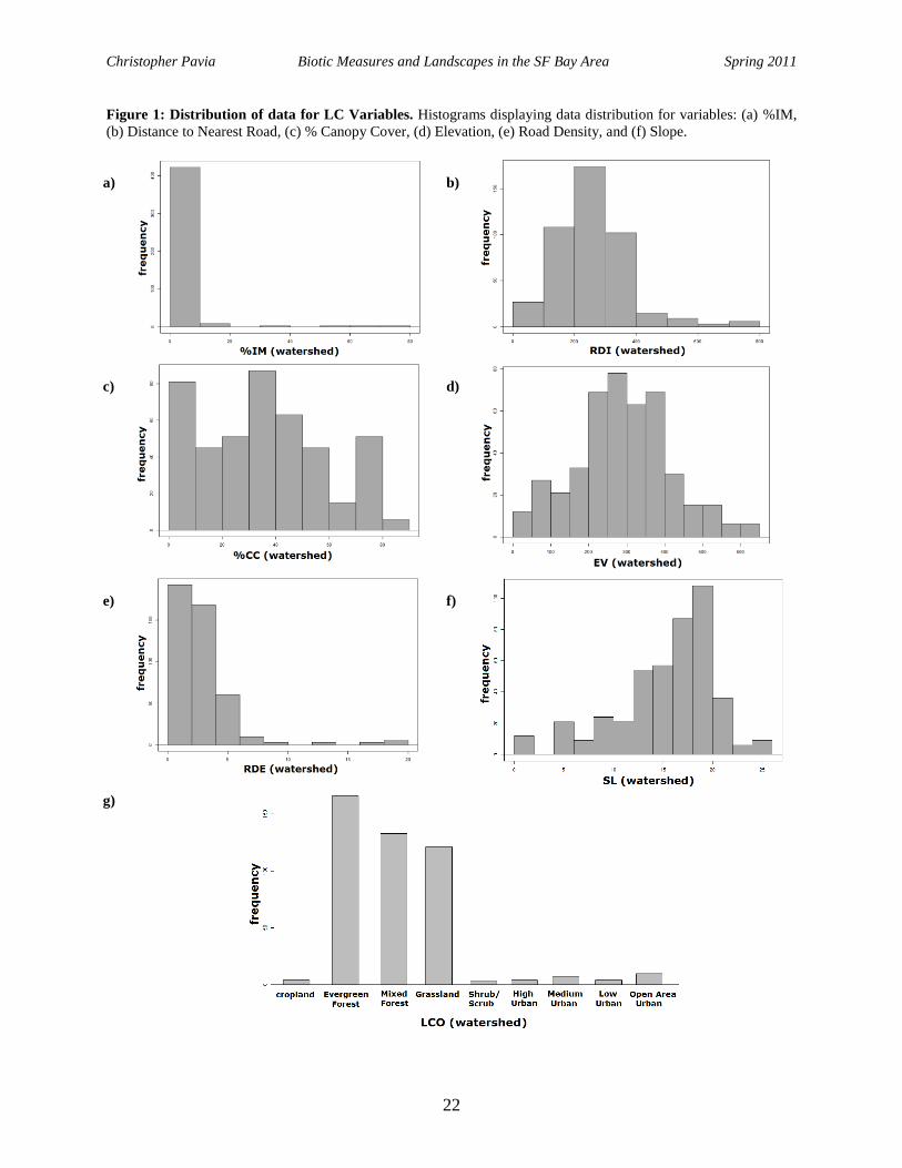
The %IM data was concentrated at the lower bound, with 95% of the data (421 of 444 sites)
below 10% impervious surface coverage. The data’s mean and median were 3.8% (± 6.8%
standard deviation) and 0.49% (Table 8, Figure 2a). %IM had a weak correlation with %CC, where
higher %IM values occurred at lower %CC values (Figure 3b, R2 = 0.1379, p < 0.000001).

Christopher Pavia Biotic Measures and Landscapes in the SF Bay Area Spring 2013
7
There were also higher %IM values at lower SL values (Figure 3f).
% Canopy Cover
%CC had peaks between 0% and 10% and between 30% and 40% coverage, while the
median was at 35% (Table 8). RDE, RDI, PD, and %IM all showed no relationship. %CC and EV
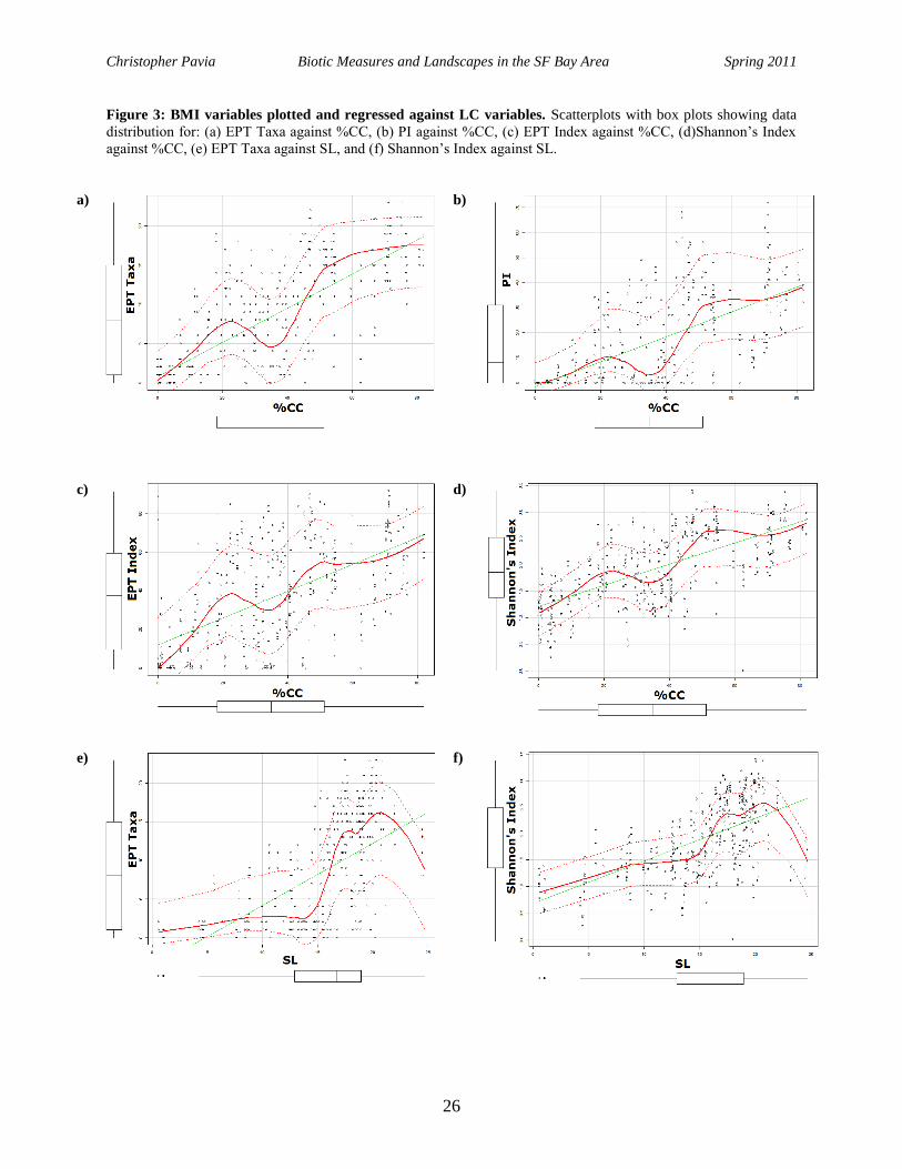
showed a semi-linear relationship (Figure 3a, R2 = 0.2922, p < 0.000001), while %CC and SL
showed a stronger correlation (Figure 3c, R2 = 0.4967, p < 0.000001).
Land Cover
Forests (67%, 297 of 444 sites) and Grasslands (27%, 119 of 444 sites) made up the bulk
of the data, with the rest of the data evenly distributed throughout all four categories of urban sites
(5%, 22 of 444 sites) (Table 8, Figure 2g).
Road Density and Road Distance
RDE was distributed mostly at the left bound, with high right-tail skewedness (Figure 2e).
The only LC variable that showed correlation with RDE was RDI, which showed an inverse
relationship (Figure 3e, R2 = 0.3892, p < 0.000001). RDI was almost normally distributed (Figure
2b), although left skewed (Table 8).
Elevation and Slope
Elevation and slope both appear normally distributed (Figure 2D and 2F). They correlated
well with each other (Figure 3d, R2 =0.5441, p < 0.000001), while EV correlated slightly with
%CC (Figure 3a, R2 = 0.2922, p < 0.000001) and SL correlated slightly with %CC (Figure 3c, R2
= 0.4967, p < 0.000001).
Relationships between Landscape and BMI variables
Christopher Pavia Biotic Measures and Landscapes in the SF Bay Area Spring 2013
8
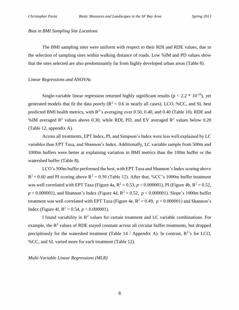
Bias in BMI Sampling Site Locations
The BMI sampling sites were uniform with respect to their RDI and RDE values, due to
the selection of sampling sites within walking distance of roads. Low %IM and PD values show
that the sites selected are also predominantly far from highly developed urban areas (Table 8).
Linear Regressions and ANOVAs
Single-variable linear regression returned highly significant results (p < 2.2 * 10-16), yet
generated models that fit the data poorly (R2 < 0.6 in nearly all cases). LCO, %CC, and SL best
predicted BMI health metrics, with R2’s averaging over 0.50, 0.40, and 0.40 (Table 10). RDE and
%IM averaged R2 values above 0.30, while RDI, PD, and EV averaged R2 values below 0.20
(Table 12, appendix A).
Across all treatments, EPT Index, PI, and Simpson’s Index were less well explained by LC
variables than EPT Taxa, and Shannon’s Index. Additionally, LC variable sample from 500m and
1000m buffers were better at explaining variation in BMI metrics than the 100m buffer or the
watershed buffer (Table 8).
LCO’s 500m buffer performed the best, with EPT Taxa and Shannon’s Index scoring above
R2 = 0.60 and PI scoring above R2 = 0.50 (Table 12). After that, %CC’s 1000m buffer treatment
was well correlated with EPT Taxa (Figure 4a, R2 = 0.53, p < 0.000001), PI (Figure 4b, R2 = 0.52,
p < 0.000001), and Shannon’s Index (Figure 4d, R2 = 0.52, p < 0.000001). Slope’s 1000m buffer
treatment was well correlated with EPT Taxa (Figure 4e, R2 = 0.49, p < 0.000001) and Shannon’s
Index (Figure 4f, R2 = 0.54, p < 0.000001).
I found variability in R2 values for certain treatment and LC variable combinations. For
example, the R2 values of RDE stayed constant across all circular buffer treatments, but dropped
precipitously for the watershed treatment (Table 14 / Appendix A). In contrast, R2’s for LCO,
%CC, and SL varied more for each treatment (Table 12).
Multi-Variable Linear Regressions (MLR)
Christopher Pavia Biotic Measures and Landscapes in the SF Bay Area Spring 2011
9
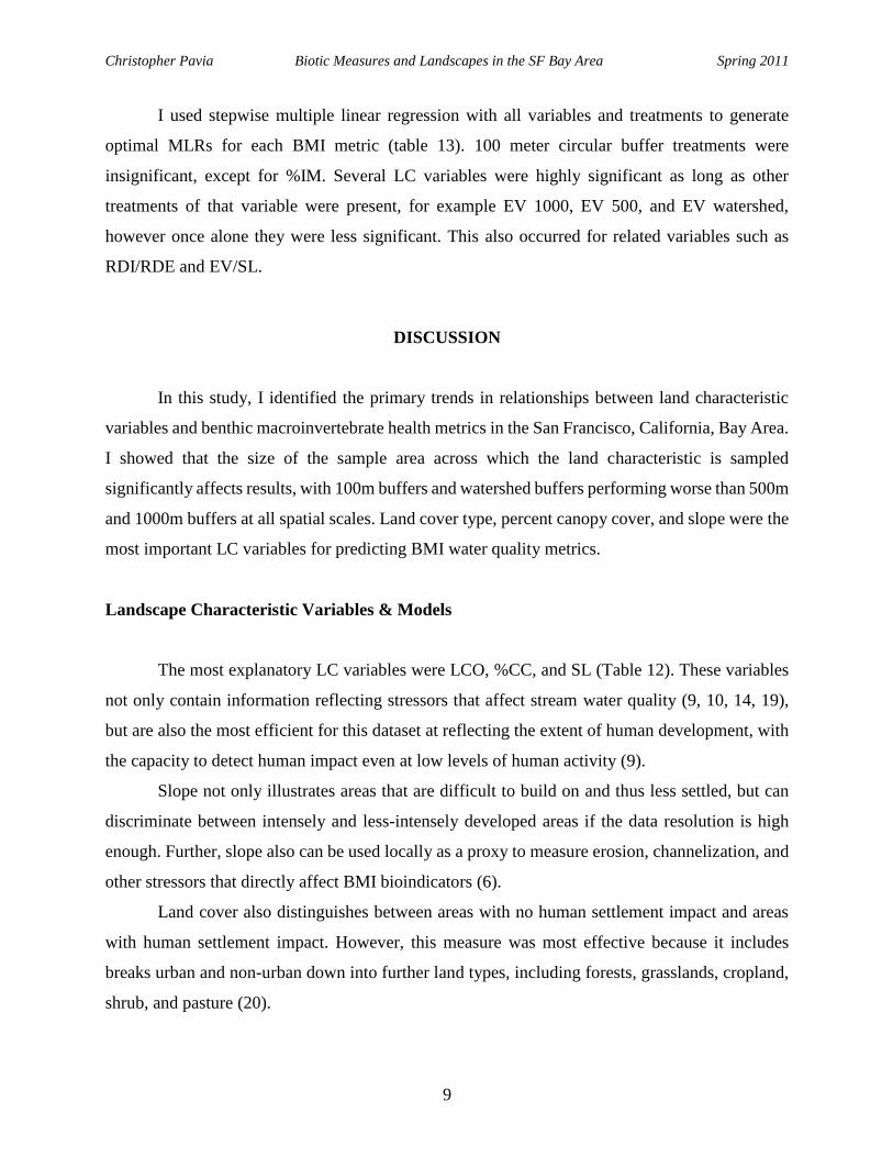
I used stepwise multiple linear regression with all variables and treatments to generate
optimal MLRs for each BMI metric (table 13). 100 meter circular buffer treatments were
insignificant, except for %IM. Several LC variables were highly significant as long as other
treatments of that variable were present, for example EV 1000, EV 500, and EV watershed,
however once alone they were less significant. This also occurred for related variables such as
RDI/RDE and EV/SL.
DISCUSSION
In this study, I identified the primary trends in relationships between land characteristic
variables and benthic macroinvertebrate health metrics in the San Francisco, California, Bay Area.
I showed that the size of the sample area across which the land characteristic is sampled
significantly affects results, with 100m buffers and watershed buffers performing worse than 500m
and 1000m buffers at all spatial scales. Land cover type, percent canopy cover, and slope were the
most important LC variables for predicting BMI water quality metrics.
Landscape Characteristic Variables & Models
The most explanatory LC variables were LCO, %CC, and SL (Table 12). These variables
not only contain information reflecting stressors that affect stream water quality (9, 10, 14, 19),
but are also the most efficient for this dataset at reflecting the extent of human development, with
the capacity to detect human impact even at low levels of human activity (9).
Slope not only illustrates areas that are difficult to build on and thus less settled, but can
discriminate between intensely and less-intensely developed areas if the data resolution is high
enough. Further, slope also can be used locally as a proxy to measure erosion, channelization, and
other stressors that directly affect BMI bioindicators (6).
Land cover also distinguishes between areas with no human settlement impact and areas
with human settlement impact. However, this measure was most effective because it includes
breaks urban and non-urban down into further land types, including forests, grasslands, cropland,
shrub, and pasture (20).
Christopher Pavia Biotic Measures and Landscapes in the SF Bay Area Spring 2011
10
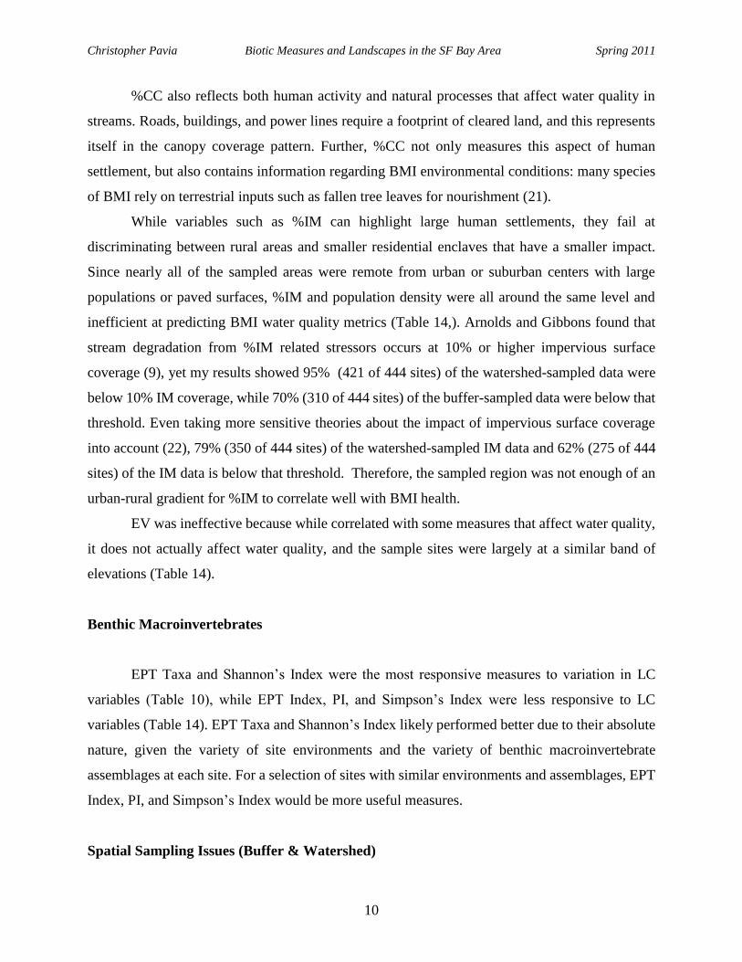
%CC also reflects both human activity and natural processes that affect water quality in
streams. Roads, buildings, and power lines require a footprint of cleared land, and this represents
itself in the canopy coverage pattern. Further, %CC not only measures this aspect of human
settlement, but also contains information regarding BMI environmental conditions: many species
of BMI rely on terrestrial inputs such as fallen tree leaves for nourishment (21).
While variables such as %IM can highlight large human settlements, they fail at
discriminating between rural areas and smaller residential enclaves that have a smaller impact.
Since nearly all of the sampled areas were remote from urban or suburban centers with large
populations or paved surfaces, %IM and population density were all around the same level and
inefficient at predicting BMI water quality metrics (Table 14,). Arnolds and Gibbons found that
stream degradation from %IM related stressors occurs at 10% or higher impervious surface
coverage (9), yet my results showed 95% (421 of 444 sites) of the watershed-sampled data were
below 10% IM coverage, while 70% (310 of 444 sites) of the buffer-sampled data were below that
threshold. Even taking more sensitive theories about the impact of impervious surface coverage
into account (22), 79% (350 of 444 sites) of the watershed-sampled IM data and 62% (275 of 444
sites) of the IM data is below that threshold. Therefore, the sampled region was not enough of an
urban-rural gradient for %IM to correlate well with BMI health.
EV was ineffective because while correlated with some measures that affect water quality,
it does not actually affect water quality, and the sample sites were largely at a similar band of
elevations (Table 14).
Benthic Macroinvertebrates
EPT Taxa and Shannon’s Index were the most responsive measures to variation in LC
variables (Table 10), while EPT Index, PI, and Simpson’s Index were less responsive to LC
variables (Table 14). EPT Taxa and Shannon’s Index likely performed better due to their absolute
nature, given the variety of site environments and the variety of benthic macroinvertebrate
assemblages at each site. For a selection of sites with similar environments and assemblages, EPT
Index, PI, and Simpson’s Index would be more useful measures.
Spatial Sampling Issues (Buffer & Watershed)
Christopher Pavia Biotic Measures and Landscapes in the SF Bay Area Spring 2011
11
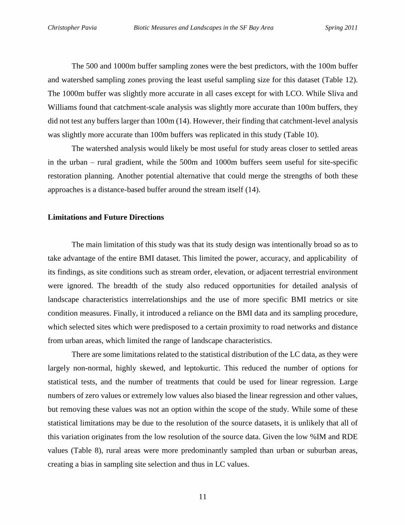
The 500 and 1000m buffer sampling zones were the best predictors, with the 100m buffer
and watershed sampling zones proving the least useful sampling size for this dataset (Table 12).
The 1000m buffer was slightly more accurate in all cases except for with LCO. While Sliva and
Williams found that catchment-scale analysis was slightly more accurate than 100m buffers, they
did not test any buffers larger than 100m (14). However, their finding that catchment-level analysis
was slightly more accurate than 100m buffers was replicated in this study (Table 10).
The watershed analysis would likely be most useful for study areas closer to settled areas
in the urban – rural gradient, while the 500m and 1000m buffers seem useful for site-specific
restoration planning. Another potential alternative that could merge the strengths of both these
approaches is a distance-based buffer around the stream itself (14).
Limitations and Future Directions
The main limitation of this study was that its study design was intentionally broad so as to
take advantage of the entire BMI dataset. This limited the power, accuracy, and applicability of
its findings, as site conditions such as stream order, elevation, or adjacent terrestrial environment
were ignored. The breadth of the study also reduced opportunities for detailed analysis of
landscape characteristics interrelationships and the use of more specific BMI metrics or site
condition measures. Finally, it introduced a reliance on the BMI data and its sampling procedure,
which selected sites which were predisposed to a certain proximity to road networks and distance
from urban areas, which limited the range of landscape characteristics.
There are some limitations related to the statistical distribution of the LC data, as they were
largely non-normal, highly skewed, and leptokurtic. This reduced the number of options for
statistical tests, and the number of treatments that could be used for linear regression. Large
numbers of zero values or extremely low values also biased the linear regression and other values,
but removing these values was not an option within the scope of the study. While some of these
statistical limitations may be due to the resolution of the source datasets, it is unlikely that all of
this variation originates from the low resolution of the source data. Given the low %IM and RDE
values (Table 8), rural areas were more predominantly sampled than urban or suburban areas,
creating a bias in sampling site selection and thus in LC values.

Christopher Pavia Biotic Measures and Landscapes in the SF Bay Area Spring 2011
12
This study also had several methodological limitations with regards to the GIS component.
The study did not calculate error accumulation, either inherent in NLCD or SWAMP datasets, or
propagated through ArcGIS analysis.
In addition, land cover type was underused relative to the other continuous data layers. The
Anderson land cover classification proposed in 1976 (23) has long become the standard land cover
classification system, but such one-dimensional systems have accumulated their share of criticism
(24 – 27).
The results in this study also point to significant potential future research. Splitting the
dataset into subsets based upon the BMI water quality data would allow more precise analysis of
specific relationships between BMI and LC values. Land cover could be better integrated into the
study by using patch dynamics to break land cover down into quantitative metrics such as patch
density, patch size, and shape indices (28), or by reclassifying continuous LC variables into
discrete, categorical variables as in suitability analysis (29, 30). Alternatively, a more focused
approach could take a single LC variable and examine its relationships to functional feeding groups
and other site characteristics such as water chemistry or the physical form of the site.
CONCLUSION
This study examined new BMI data available for the San Francisco, California, Bay Area.
Sites with high and low BMI scores often shared the same range of landscape characteristic values.
This reinforces that multiple variables need to be considered in any analysis of BMI scores (19).
Sites may possess landscape characteristics that would create a good environment for benthic
macroinvertebrates, but which are counterbalanced by the shortcomings of another LC variable
(31).
Higher scores of %CC, slope, and non-urbanized values of LCO were the main factors
associated with high BMI scores, particularly Shannon’s Index and EPT Taxa. This suggests
expanding planting of tree cover over and near non-vegetated creeks could improve stream water
quality and assemblage health (31, 32) and would also improve property values (33). Given the
presence of previous restoration of culverted and underground creeks in the Berkeley area (34),
and the presence of creek stewardship groups like The Urban Creeks Council, Friends of Five
Christopher Pavia Biotic Measures and Landscapes in the SF Bay Area Spring 2011
13
Creeks, The Watershed Project, and the East Bay Chapter, these findings or findings from future
research may prove useful to these groups for decision making.
ACKNOWLEDGEMENTS
This research was made possible through the support of the Resh Lab and its members,
especially Justin Lawrence, and support from the Surface Water Ambient Monitoring Program,
particularly Kevin Lunde. I thank the UC Berkeley teaching staff of ES100 and ES196, especially
Patina Mendez, for their comments and editing assistance.
REFERENCES
(1) McDonnell, M., and Pickett, S., Ecosystem Structure and Function Along Urban Rural
Gradients - an Unexploited Opportunity for Ecology, Ecology, 71,1232-1237, 1990.
(2) McCreary, S., Twiss, R., Warren, B., White, C., Huse, S., Gardels, K., and Roques, D., Land-
use Change and Impacts on the San-Francisco Estuary - a Regional Assessment with
National Policy Implications, Coastal Management, 20, 219-253, 1992.
(3) Meyer, J., Paul, M., and Taulbee, W., Stream ecosystem function in urbanizing landscapes,
Journal of the North American Benthological Society 24,602-612, 2005.
(4) Walsh C., Roy, A., Feminella, J., Cottingham, P., Groffman, P., and Morgan, R., The urban
stream syndrome: current knowledge and the search for a cure, Journal of the North
American Benthological Society, 24, 706-723, 2005.
(5) Poff, N. L., Allan, J. D., Bain, M. B., Karr, J. R., Prestegaard, K. L., Richter, B. D., Sparks,
R. E., and Stromberg, J. C., The natural flow regime, Bioscience 47, 769-784, 1997.
(6) Barbour, M.T., Gerritsen, J., Snyder, B.D., and Stribling, J.B., Rapid bioassessment protocols
for use in streams and wadeable Rivers: periphyton, benthic macroinvertebrates and fish.
2nd Edition. EPA 841-B-99-002, Office of Water, U.S. Environmental Protection
Agency, 1999.
(7) Resh, V., Norris, R., and Barbour , M., Design and Implementation of Rapid Assessment
Approaches for Water-Resource Monitoring using Benthic Macroinvertebrates Rid D-
2741-2009, Australian Journal of Ecology, 20, 108-121, 1995.
(8) Resh, V. H., and Johnson, J. K., Editors Rosenberg, D.M. and Resh, V.H., Rapid assessment
approaches to biomonitoring using benthic macroinvertebrates, 1993.
(9) Arnold, C., Gibbons, C., Impervious surface coverage - The emergence of a key
environmental indicator, Journal of the American Planning Association, 62, 243-258,
1996.
(10) Tate, C. M., Cuffney, T. F., McMahon, G., Giddings, E. M. P., Coles, J. F., and Zappia, H.,
Use of an urban intensity index to assess urban effects on streams in three contrasting
environmental settings, American Fisheries Society Symposium, 47, 291-315, 2005.

Christopher Pavia Biotic Measures and Landscapes in the SF Bay Area Spring 2011
14
(11) McMahon, G. and Cuffney, T. F., Quantifying urban intensity in drainage basins for
assessing stream ecological conditions, JAWRA Journal of the American Water
Resources Association, 36, 1247–1261, 2000.
(12) Bressler, D. W., Paul , M. J., Purcell , A. H., Barbour , M. T., Rankin, E. T., and Resh,V. H.,
Assessment Tools for Urban Catchments: Developing Stressor Gradients, Journal of the
American Water Resources Association, 45,291-305, 2009.
(13) Kearns, F.R., Kelly, N. M., Carter, J. L., and Resh, V. H., A method for the use of landscape
metrics in freshwater research and management, Landscape Ecology, 20,113–125, 2005.
(14) Sliva, L., Williams, D., Buffer zone versus whole catchment approaches to studying land
use impact on river water quality, Water research, 35, 3462-3472, 2001.
(15) Carter, J. L., Purcell, A. H., Fend, S. V., and Resh, V. H., Development of a local-scale
urban stream assessment method using benthic macroinvertebrates: an example from the
Santa Clara Basin, California, Journal of the North American Benthological Society,
28(4), 1007-1021, 2009.
(16) Lawrence, J. E., Lunde, K. B., Mazor, R. D., Bêche, L. A., McElravy, E. P., and Resh, V.
H., Long-term macroinvertebrate responses to climate change: implications for biological
assessment in mediterranean-climate streams, Journal of the North American
Benthological Society, 29(4), 1424-1440, 2010.
(17) Lunde, K. B., "Investigations of Altered Aquatic Ecosystems: Biomonitoring, Disease, and
Conservation: Chapter 5: Identifying reference sites and quantifying biological variability
within the benthic macroinvertebrate community," Dissertation, University of California,
Berkeley, 2011.
(18) Openshaw, S., The Modifiable Areal Unit Problem, Concepts and Techniques in Modern
Geography, 38, 1-41, 1984.
(19) Purcell, H. A., Bressler, D. W., Paul, M. J., Barbour, M. T., Rankin, E. T., Carter, J. L., and
Resh, V. H., Assessment Tools for Urban Catchments: Developing Biological Indicators
Based On Benthic Macroinvertebrates, Journal of the American Water Resources
Association, 45, 306-319, 2009.
(20) U.S. Geological Survey, NLCD 2001 Land Cover Version 2.0 Metadata, National Seamless
Server, U.S. Geological Survey and U.S. Department of the Interior, 2001.
<http://seamless.usgs.gov/>
(21) Lake, P. S., Bond, N., and Reich, P., Linking ecological theory with stream restoration,
Freshwater Biology, 52, 597-615, 2007.
(22) Schueler, T. R., Fraley-McNeal, L., and Cappiella ,K., Is Impervious Cover Still Important?
Review of Recent Research, Journal of Hydrological Engineering, 14, 309-315, 2009.
(23) Anderson, J. R., Hardy, E. E., Roach, J. T., and Witmer, R. E., Land use and land cover
classification systems for use with remote sensor data. Professional Paper 964., U.S.
Geological Service, 1976.
(24) Klijn, F., and Udo de Haes, H. A., A hierarchical approach to ecosystems and its
implications for ecological land classification, Landscape Ecology, 9, 89-104, 1994.
(25) Hong, S.-K., Kim, S., Cho, K.-H., Kim, J.-E., Kang, S., and Lee, D., Ecotope mapping for
landscape ecological assessment of habitat and ecosystem, Ecological Research, 19, 131-
139, 2004.
(26) Band, L. E., Cadenasso, M. L., Grimmond, C. S., Grove, J. M., and Pickett S. T.,
Heterogeneity in Urban Ecosystems: Patterns and Process, in Lovett, G. M., Turner, M.

Christopher Pavia Biotic Measures and Landscapes in the SF Bay Area Spring 2011
15
G., Jones, C. G., and Weathers, K. C., Ecosystem Function in Heterogeneous
Landscapes, 257-278, 2005.
(27) Cadenasso, M. L., Pickett, S. T. A., and Schwarz, K., Spatial heterogeneity in urban
ecosystems: reconceptualizing land cover and a framework for classification, Frontiers in
Ecology and the Environment, 5, 80-88, 2007.
(28) Host, G. E., Schuldt, J., Ciborowski, J. J. H., Johnson, L. B., Hollenhorst, T., and Richards,
C., Use of GIS and remotely sensed data for a priori identification of reference areas for
Great Lakes coastal ecosystems, International Journal of Remote Sensing, 26(23), 5325–
5342, 2005.
(29) Malczewski, J., GIS-based land-use suitability analysis: a critical overview, Progress in
Planning, 62, 3-65, 2004.
(30) Xiao, H., and Ji, W., Relating landscape characteristics to non-point source pollution in
mine waste-located watersheds using geospatial techniques, Journal of Environmental
Management, 82, 111–119, 2004.
(31) Basnyat, P., Teeter, L., Flynn, K., and Lockaby, B. G., Relationships Between Landscape
Characteristics and Nonpoint Source Pollution Inputs to Coastal Estuaries, Environmental
Management, 23(4), 539–549, 1999.
(32) Basnyat, P., Teeter, L. D., Lockaby, B. G., and Flynn, K. M., The use of remote sensing and
GIS in watershed level analyses of non-point source pollution problems, Forest Ecology
and Management, 128, 65-73, 2000.
(33) Kadish, J., and Netusil, N. R., Valuing vegetation in an urban watershed, Landscape and
Urban Planning, 104,59-65, 2012.
(34) Pinkham, R, Daylighting: New Life For Buried Streams, Rocky Mountain Institute, 2000.

Christopher Pavia Biotic Measures and Landscapes in the SF Bay Area Spring 2011
16
Table 1. BMI metrics used in this study. These metrics are standard metrics commonly used in benthic
macroinvertebrate studies that are easy to calculate and use, while communicating different information.
Metric Description Use
EPT Taxa
(abundance)
Total number of Ephemeroptera,
Plecoptera, and Trichoptera (EPT) found
Indicate general level of water quality
at site.
EPT Index
(richness)
Number of different taxa of
Ephemeroptera, Plecoptera, and
Trichoptera (EPT) given as % of total
Indicate general level of water quality
at site.
BMI richness (PI) Number of different taxa of Benthic
Macroinvertebrates found given as % of
total
In combination with EPT data, helps
identify whether EPT data results are
due to water pollution conditions or
environmental conditions
Shannon-Weaver
Diversity Index
The proportion of a single species relative
to the total number of species, multiplied
by natural logarithm of that proportion.
Diversity indices account for
abundance (how many individuals
there are), richness (how many
species there are), and evenness (how
a species is distributed) of a single
species in relation to the community.
Simpson’s Diversity
Index
The reciprocal of the summed squared
proportions of a single species relative to
the total number of species.

Christopher Pavia Biotic Measures and Landscapes in the SF Bay Area Spring 2011
17
Table 2: LC variables used in this study. These variables were freely available as part of the NLCD on the National
Map Viewer ( http://nationalmap.gov/viewer.html ). * SRTM = Shuttle Radar Topography Mission, USGS = US
Geological Survey, DEM = Digital Elevation Model.
Landscape
Variable Abbreviation Units of Variable Associated Factors
Percent Canopy
Cover
%CC Area with canopy cover /
total area of cell
Terrestrial inputs, temperature
effects through shade
Road Density RDE km of road / km2 of area Pollutants, run-off, vibrational
disturbance
Distance to Nearest
Road
RDI Distance to nearest road from
cell center point in meters
Pollutants, run-off, vibrational
disturbance
Elevation EV Distance from SRTM*
USGS DEM designated zero
elevation (sea level) in
meters.
Stream order, stream
geomorphology
Percent Impervious
Surface Coverage
%IM Area with impervious surface
cover / total area of cell
Urbanization impacts, run-off
Population Density PD People per mile2 Urbanization impacts
Slope SL Degrees rise per cell Stream order, stream
geomorphology, erosion,
channelization

Christopher Pavia Biotic Measures and Landscapes in the SF Bay Area Spring 2011
18
Table 3: Median mean values, χ², and p-values of landscape variables per transect and Kruskal-Wallis Test
Result (df = 3, crit value = 7.815). This test shows that while there are differences in the landscape variables between
transect sampling methods, these differences are not significant. (* = significant results; x = groups were similar,✝ =
groups were different).
Medians
Three Transect
Samples
X (Single
Transect) Result (χ²) p-value Result
%CC 27.2 24.0 0.2362 .9722 ✝
RDE 2.90 4.06 37.50 < .00001 x *
RDI 123 60.9 17.65 .0005 x *
EV 135 131 0.9657 .8095 x *
%IM 1.31 4.43 28.48 < .00001 x *
PD 93.8 60.0 3.221 .3588 ✝
SL 12.2 13.0 4.52 .2100 ✝

Christopher Pavia Biotic Measures and Landscapes in the SF Bay Area Spring 2011
19
Table 4: Normality of data per landscape variable and treatment type. All data were explicitly non-normal,
although watershed treatments were more normal than circular buffer treatments. All p-values are less than 0.00001
unless otherwise stated. W = Shapiro-Wilks statistic denoting degree of normality with 0 = non-normal and 1 =
perfectly normally distributed. (✝ = potentially normal, ✝✝ = relatively normal).
Distance of
Buffer
Circular Buffer Treatment Watershed
Treatment 100m 500m 1000m
Population
Density
W = 0.389
W = 0.5377
W = 0.5982 W = 0.3487
% Impervious
Cover
W = 0.6977
W = 0.6896
W = 0.7059
W = 0.3754
% Canopy
Cover W = 0.8552
✝
W = 0.8603✝
W = 0.8841✝
W = 0.9598✝✝
Road Density W = 0.8452✝
W = 0.8456✝
W = 0.845✝
W = 0.5974
Road Distance W = 0.5375
W = 0.8281
✝ W = 0.9353
✝✝ W = 0.9252
✝✝
Elevation W = 0.8345✝
W = 0.8699✝
W = 0.8974✝
W = 0.9885✝✝
p-value = 0.001434
Slope W = 0.8961✝
W = 0.9396✝✝
W = 0.9384✝✝
W = 0.92✝✝

Christopher Pavia Biotic Measures and Landscapes in the SF Bay Area Spring 2011
20
Table 5: Numerical summaries of LC variable data. STD = standard deviation, cv = coefficient of variation
(standard deviation divided by mean), IQR = interquartile range. Skew measures the distortion of a probability
distribution’s spread from the mean; kurtosis measures how distorted a probability distribution’s magnitude is.
Landscape
Variable
Sampling
Buffer Size mean STD median IQR cv skew kurtosis
% Canopy
Cover
0100m 32.6 30.1 22.1 60.5 0.920 0.368 -1.5
0500m 29.6 28.3 20.0 47.2 0.955 0.539 -1.2
1000m 28.8 26.7 20.5 43.4 0.928 0.592 -0.95
watershed 35.3 22.5 34.8 33.0 0.638 0.185 -0.89
Road Density 0100m 5.44 4.75 3.66 5.79 0.873 1.20 0.518
0500m 5.38 4.68 3.49 5.68 0.868 1.19 0.468
1000m 5.26 4.55 3.44 5.50 0.865 1.16 0.338
watershed 3.01 2.74 2.26 1.98 0.909 3.89 18.4
Distance to
Nearest Road
0100m 64.3 87.1 36.0 26.9 1.35 3.68 16.0
0500m 115. 88.2 109 97.1 0.765 2.06 6.57
1000m 159. 109. 145 141. 0.686 0.831 0.441
watershed 264. 124. 263 150. 0.469 1.11 3.28
Elevation 0100m 97.5 90.1 73.3 111. 0.925 1.87 5.23
0500m 120. 102. 106 119. 0.844 1.60 3.87
1000m 139. 109. 135 135. 0.782 1.35 2.91
watershed 292. 126. 290 163. 0.433 0.0907 0.0162
% Impervious
Cover
0100m 10.9 16.5 2.79 12.5 1.52 1.73 1.98
0500m 12.2 18.6 1.58 16.2 1.52 1.52 0.965
1000m 12.3 18.4 1.26 19.2 1.49 1.52 1.10
watershed 3.76 9.58 0.490 4.37 2.55 5.36 31.2
Population
Density
0100m 1205. 3398. 69.9 743. 2.82 5.18 31.3
0500m 1120. 2541. 93.9 849. 2.12 3.26 12.8
1000m 1246. 2344. 111 1512. 1.88 2.72 8.49
watershed 397. 1096. 64.9 355. 2.76 6.11 43.5
Slope 0100m 8.07 7.14 6.26 10.5 0.884 0.942 0.257
0500m 10.4 7.36 10.9 12.6 0.709 0.277 -0.947
1000m 10.9 6.89 12.3 11.9 0.630 -0.0545 -1.18
watershed 15.4 5.02 16.7 5.98 0.326 -1.01 0.743

Christopher Pavia Biotic Measures and Landscapes in the SF Bay Area Spring 2011
21
Table 6: Breakdown of land cover types per treatment. Buffer-sampled data were consistent between the three
distances, excepting Urban – Open, while watershed-sampled data had less data spread across multiple categories.
Treatments
Land Cover Types 100m 500m 1000m Watershed
Cropland 7% 4% 3% 1%
Forest - Evergreen 22% 26% 26% 37%
Forest - Mixed 11% 11% 14% 30% Grassland 15% 28% 28% 27% Pasture - - 1% -
Shrub 1% 2% 2% 1% Urban - High - 1% - 1%
Urban - Medium 10% 14% 14% 1%
Urban - Low 7% 6% 5% 1%
Urban – Open 25% 9% 7% 2% Woody Wetlands 1% - - -
Christopher Pavia Biotic Measures and Landscapes in the SF Bay Area Spring 2011
22
Figure 1: Distribution of data for LC Variables. Histograms displaying data distribution for variables: (a) %IM,
(b) Distance to Nearest Road, (c) % Canopy Cover, (d) Elevation, (e) Road Density, and (f) Slope.
a)
b)
c)
d)
e)
f)
g)

Christopher Pavia Biotic Measures and Landscapes in the SF Bay Area Spring 2011
23
Figure 2: Correlations between LC variables. Scatterplots of the watershed-sampled LC variables against one
another, with a) %CC against EV, (b) %IM against %CC, (c) %CC against SL, (d) EV against SL, (e) RDE against
RDI, and (f) SL against %IM.
a)
b)
c)
d)
e)
f)

Christopher Pavia Biotic Measures and Landscapes in the SF Bay Area Spring 2011
24
Table 7: R2 values of linear regression for LCO, %CC, and SL. Light blue cells have an R2 above 0.50, light green
cells have an R2 above 0.40, light orange cells have an R2 above 0.30, and dark red shaded squares have an R2 below
0.20.
Adjusted R2
Sampling
Zone Sizes
EPT
Taxa
EPT
Index
Shannon’s
Index
Simpson’s
Index PI
Average
R2
LC
O
100.00 0.43 0.35 0.46 0.40 0.38 0.40
500.00 0.61 0.49 0.60 0.47 0.58 0.57
1000.00 0.63 0.45 0.58 0.43 0.55 0.55
wtr 0.53 0.27 0.44 0.32 0.41 0.42
Average R2 0.55 0.39 0.52 0.40 0.48
CC
100.00 0.38 0.41 0.44 0.32 0.40 0.39
500.00 0.50 0.45 0.52 0.36 0.52 0.48
1000.00 0.53 0.45 0.52 0.36 0.53 0.49
wtr 0.49 0.33 0.43 0.33 0.39 0.41
Average R2 0.48 0.41 0.48 0.34 0.46
SL
100.00 0.27 0.32 0.34 0.24 0.28 0.29
500.00 0.44 0.42 0.51 0.39 0.43 0.44
1000.00 0.49 0.45 0.54 0.42 0.47 0.48
wtr 0.33 0.28 0.34 0.29 0.27 0.31
Average R2 0.38 0.37 0.43 0.34 0.36
DE
100.00 0.43 0.30 0.41 0.37 0.30 0.37
500.00 0.43 0.31 0.41 0.37 0.31 0.37
1000.00 0.44 0.31 0.42 0.38 0.31 0.38
wtr 0.16 0.12 0.18 0.20 0.12 0.15
Average R2 0.37 0.26 0.36 0.33 0.26
%IM
100.00 0.34 0.34 0.39 0.42 0.24 0.34
500.00 0.39 0.34 0.40 0.38 0.28 0.36
1000.00 0.41 0.35 0.41 0.39 0.29 0.37
wtr 0.14 0.12 0.17 0.19 0.10 0.14
Average R2 0.32 0.29 0.34 0.34 0.23
DI
100.00 0.06 0.04 0.05 0.03 0.04 0.05
500.00 0.26 0.15 0.23 0.17 0.18 0.21
1000.00 0.36 0.19 0.32 0.25 0.25 0.28
wtr 0.09 0.06 0.08 0.08 0.07 0.08
Average R2 0.19 0.11 0.17 0.13 0.13
EV
100.00 0.08 0.15 0.11 0.07 0.11 0.10
500.00 0.13 0.20 0.17 0.12 0.17 0.16
1000.00 0.19 0.25 0.24 0.16 0.22 0.22
wtr 0.21 0.21 0.19 0.12 0.22 0.20
Average R2 0.15 0.20 0.18 0.12 0.18

Christopher Pavia Biotic Measures and Landscapes in the SF Bay Area Spring 2011
25
PD
100.00 0.09 0.06 0.06 0.04 0.06 0.07
500.00 0.19 0.13 0.16 0.13 0.13 0.15
1000.00 0.26 0.18 0.22 0.18 0.18 0.21
wtr 0.11 0.09 0.13 0.14 0.08 0.11
Average R2 0.16 0.12 0.15 0.12 0.11
Christopher Pavia Biotic Measures and Landscapes in the SF Bay Area Spring 2011
26
Figure 3: BMI variables plotted and regressed against LC variables. Scatterplots with box plots showing data
distribution for: (a) EPT Taxa against %CC, (b) PI against %CC, (c) EPT Index against %CC, (d)Shannon’s Index
against %CC, (e) EPT Taxa against SL, and (f) Shannon’s Index against SL.
a)
b)
c)
d)
e)
f)

Christopher Pavia Biotic Measures and Landscapes in the SF Bay Area Spring 2011
27
Table 8: Stepwise minimal multiple linear regression. The stepwise regression was calculated manually, with non-
significant factors with largest p-values removed first, then with least significant factors duplicating a single LC
variable removed until a single model with only one treatment for each LC variable was left. All models have p-value
< .000001.
BMI
Metric
LC Variables used in MLR model Adjusted
R2 Circular Buffer Watershed
EPT Taxa CC 500
RDI 1000
RDE 1000
EV watershed
0.6428
EPT Index IM 0100
CC 500
RDI 500
RDE 1000
EV watershed
0.5476
Shannon’s
Index
CC 500
EV 500
RDI 1000
SL 1000
RDE watershed
0.6452
Simpson’s
Index
IM 100
CC 500
SL watershed
0.5510
PI CC 500
SL 1000
RDE watershed
IM watershed
0.5895