ber- and com-way of channel- compliance evaluation

H I G H S P E E D D E S I G N WH

IT

EP

AP

ER

w w w . m e n t o r . c o m / h y p e r l y n x

BER- AND COM-WAY OF CHANNEL-COMPLIANCE EVALUATION: WHAT ARE THE SOURCES OF DIFFERENCES?

VLADIMIR DMITRIEV-ZDOROV, MENTOR GRAPHICSCHUCK FERRY, MENTOR GRAPHICSCHRISTIAN FILIP, MENTOR GRAPHICSALFRED P. NEVES, WILD RIVER TECHNOLOGY

Originally presented at DesignCon 2016

Reprinted with permission from UB Media

ABSTRACTWe analyze the computational procedure specified for Channel Operation Margin

(COM) and compare it to traditional statistical eye/BER analysis. There are a number of

differences between the two approaches, ranging from how they perform channel

characterization, to how they consider Tx and Rx noise and apply termination, to the

differences between numerical procedures employed to convert given jitter and

crosstalk responses into the vertical distribution characterizing eye diagrams and BER.

We show that depending on the channel COM may potentially overestimate the effect

of crosstalk and, depending on a number of factors, over- or underestimate the effect

of transmit jitter, especially when the channel operates at the rate limits. We propose a

modification to the COM procedure that eliminates these problems without

considerable work increase.

w w w. m ento r.co m / hy p er l y n x2

BER and COM Channel Compliance

INTRODUCTIONSince the IEEE 802.3bj 100 Gb/s Backplane Ethernet standard has been officially approved, Channel Operating

Margin (COM) will likely become an important quality-evaluation method for SERDES links. Although COM was

preceded by a long history of eye/BER evaluation techniques, those methods have never been officially

standardized. Different tools used their own smart approaches to find a channel characterization response, to select

the optimal sampling location and properly center the eye or BER diagram on the plot, to find optimal equalization

parameters, and to evaluate the effect of ISI, jitter noise, and crosstalk. There is an IBIS standard (IBIS 5.0 to 6.2) that

describes the use of Algorithmic Model Interface (IBIS-AMI) models, but it mostly defines the rules describing how a

simulation platform interacts with the model libraries, calls their interface functions, forms inputs, and reads the

output parameters. Overall, many decisions – especially those regarding channel characterization, waveform

processing, data accumulation, and impairment handling, are left for the developers. Not surprisingly, among many

tools available on the market, we can hardly find two that produce identical results and in some cases the

differences can be significant.

It appears therefore that one of the goals for COM was to minimize ambiguity in finding the signal/noise ratio, a

measure closely related to BER. COM starts from a set of S-parameters describing victim and aggressors’ channels. It

doesn’t employ time-domain responses directly, as do many tools that run SPICE-level simulation considering non-

linear models of Tx and Rx buffers. Instead, after a series of transformations, it finds the effective transfer function of

the channel and converts it into a time response by IFFT. This way, it avoids a great deal of ambiguity caused by the

SPICE type of modeling and simulation. For a given operating mode all of the necessary parameters needed to

calculate COM are defined within, that minimizes any ambiguity. These parameters include symbol rate, number of

signaling levels, package parameters, impedance mismatch, transmit and receive noise, equalization types, the

number and the limits for tap coefficients, jitter characteristics, and more. It even goes into such details as required

frequency limits and resolution for S-parameters, the number of samples per bit in the impulse response, and

meshing used when calculating probability mass functions describing the distribution of the eye density at the

chosen cross-section.

Mathematically, COM is equivalent to statistical analysis, but performs it only for one vertical cross-section of the

eye diagram that corresponds to the “best” sampling time. Therefore, it is reasonable to compare COM with

statistical eyes, rather than with bit-by-bit analysis which is often unable to provide sufficient sample size. Such a

comparison was made previously in a number of works [6, 7, and 8]. Most of them indicate that although both

metrics reliably distinguish high- and low-quality channels, the “border” cases remain inconclusive since the

compliance results do not agree. The authors give examples of false-positive and false-negative cases and try to

explain the difference by certain features of the links that differently affect the BER and COM numbers. We don’t

think, however, that a fair comparison is possible when we compare two flows where the first is non-standardized

(BER) and the second follows precise instructions (COM). What may be more reasonable is an incremental

comparison between BER and COM, which assumes that every computational step starts from identical input.

There are many items on which BER and COM may disagree, and we will analyze them in Section I. We’ll show that

most of these discrepancies are caused by different assumptions, or by different input data. There are only two

aspects of the analysis where we believe that COM makes some oversimplifications affecting the accuracy of the

results. This is where it computes contributions from the input jitter and crosstalk. We’ll discuss the assumptions

and their potential effects on jitter evaluation in Section II. In Section III we suggest a more accurate way of finding

crosstalk contribution. In Section IV we provide a simple method to calculate COM from eye-density and BER plot

measurements. In Section V we perform a series of experiments with a set of S-parameters generated from

experimental topologies mimicking the behavior of a variety of possible real-life designs. The collected results are

post-processed and used to estimate the error introduced by the simplifying assumptions made in the COM

algorithm for jitter and crosstalk computations. Finally, in the last section we present our conclusions.



I. THE MAIN SOURCES OF DIFFERENCE BETWEEN BER AND COMGoing through the steps constituting the BER and COM flows, we can identify a number of reasons causing

differences between results:

1. Channel characterization. Many EDA tools perform a detailed circuit simulation to find the response

characterizing the channel. For example, they can find an “edge” response, showing the transition from one

logical state to another. Or, they can apply a known periodic pattern (PRBS) and then find an equivalent

channel’s response by deconvolution. In these cases, they consider non-linearity of the buffers, described by

non-LTI IBIS models or by general SPICE-type sub-circuits, possibly with a transistor-level description of the

buffers. In this case, the response they measure at the receiver pins is affected by non-linear models, and may

contain the effect of common mode converted into differential at the receiver end. COM starts from

S-parameters of the bare channel, and completely ignores non-LTI and common-mode effects.

2. Since COM doesn’t use device models, it doesn’t know the exact package parameters. “Packages” in COM are

“template approximations” of those that exist in devices, containing shunt capacitors and transmission lines.

3. For similar reasons, COM doesn’t know the actual termination conditions that exist on both sides of the

channel. In most cases, it assumes 55-ohm resistive termination, which is slightly different from 50-ohm

S-parameter normalization impedance.

4. COM considers a receiver noise filter, with a flat bandwidth of 75% of the data rate. Most eye/BER analyzers

don’t have the characteristics of this filter and don’t apply it.

5. In COM, the Tx equalizer has only one pre-tap and one post-tap, with a setup limit on the cursor values. Since

the actual device might have a different architecture, its model (e.g., IBIS AMI) is likely to allow for different

settings.

6. CTLE used in COM is consistent with common practice, but optimization is performed for DC gain only. The

poles’ frequencies are predefined for a given operation mode. If we allow full optimization of CTLE

parameters, the result will likely be different.

7. In the COM flow, Gaussian and dual-Dirac transmit jitter is computed by linearizing the pulse response and

taking its slope at the selected sample points. Accurate statistical analysis requires a different approach. The

effect of ISI and peak distortion is also affected by the input jitter; that’s why accurate statistical analysis

computes the distribution that includes ISI and transmit jitter simultaneously. We’ll discuss this in more detail

below, and also in Section II.

8. In the COM procedure, optimization of equalizers’ parameters is made by considering a further simplified

metric called FOM (figure of merit), to reduce the optimization time. However, with additional assumptions,

e.g., regarding Gaussian distribution of all “noise” contributions, there is a considerable difference between the

predicted (FOM) and the final (COM) measure. We cannot be sure that the choice of equalization parameters

that gives us the best FOM also gives the best COM.

9. Signal-to-noise ratio of the transmitter is rarely considered by BER analyzers. The same is true for receive noise.

10. In COM, the contribution from aggressors is taken with the worst possible phase combinations, which may

cause crosstalk overestimation. We’ll address this issue in Section III.

11. Some of the operating modes in COM assume an error correction mechanism (FEC) and measure the noise

amplitude against the larger BER threshold. This may not be the case for many BER evaluation tools.

Most of the reasons listed above can be addressed by properly adjusting the data used in BER analysis. For

example, we can find the channel response by repeating the COM flow: start from S parameters, find contributions

from every driver, including all aggressors, convert partial 4-port parameters into differential-only mode, add

packages as defined in COM, apply termination and convert the 2-port model into a scalar transfer function, then

apply the receiver noise filter. The resulting function can be converted into step or pulse response by IFFT, and

used in the eye/BER simulation tool as shown in Fig.1.



With the non-equalized response taken from the COM engine, we can allow the eye/BER simulator to find its own

settings for feed-forward equalization, CTLE, and DFE, or take those chosen by the COM approach when finding the

best “figure of merit”. Finally, we can add the Tx and Rx noise defined by COM into eye/BER analysis.

These issues require deeper consideration. When finding noise contribution from jitter by response linearization, we

may end up with over or underestimation of jitter, which depends on the shape of the response and the chosen

sampling position. Second, the effect of jitter must be searched by analyzing the edge response (not pulse — i.e.,

bit — response) because transmit jitter changes the distance between the edges and therefore affects the shape

of the “pulse” response itself. We analyze this issue later in Section II. Regarding crosstalk, it would be more

reasonable to assume that relative phases are random and have uniform distribution. With that, we can find the

effective noise PDFs for different phases within 1UI and then find the average PDF by integrating over the unit

interval.

Fig.1 COM to Eye/BER analysis flow



II. TRANSMIT JITTER EVALUATION: RIGOROUS WAY VERSUS COM-WAYTHE EFFECT OF RESPONSE LINEARIZATION

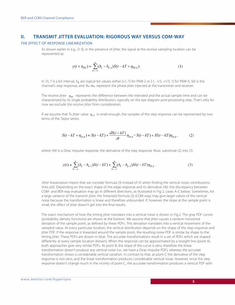
As shown earlier in e.g., [1-3], in the presence of jitter, the signal at the receive sampling location can be

represented as:

In (1), T is a bit interval, bk are logical bit values, either [+1,-1] for PAM-2 or [-1, -1/3, +1/3, 1] for PAM-4, S(t) is the

channel’s step response, and represent the phase jitter injected at the transmitter and receiver.

The receive jitter represents the difference between the intended and the actual sample time and can be

characterized by its single probability distribution, typically on the eye diagram post-processing step. That’s why for

now we exclude the receive jitter from consideration.

If we assume that Tx jitter value is small enough, the samples of the step response can be represented by two

terms of the Taylor series:

where H(t) is a Dirac impulse response, the derivative of the step response. Now, substitute (2) into (1):

Jitter linearization means that we consider formula (3) instead of (1) when finding the vertical noise contributions

(into y(t)). Depending on the exact shape of the edge response and its derivative H(t), the discrepancy between

COM- and BER-way evaluation may go in different directions, as illustrated in Fig 2, cases A-C below. Sometimes, for

a large variance of the transmit jitter, the linearized formula (3) (COM way) may give larger values of the vertical

noise because the transformation is linear and therefore unbounded. If, however, the slope at the sample point is

small, the effect of jitter doesn’t get into the final results.

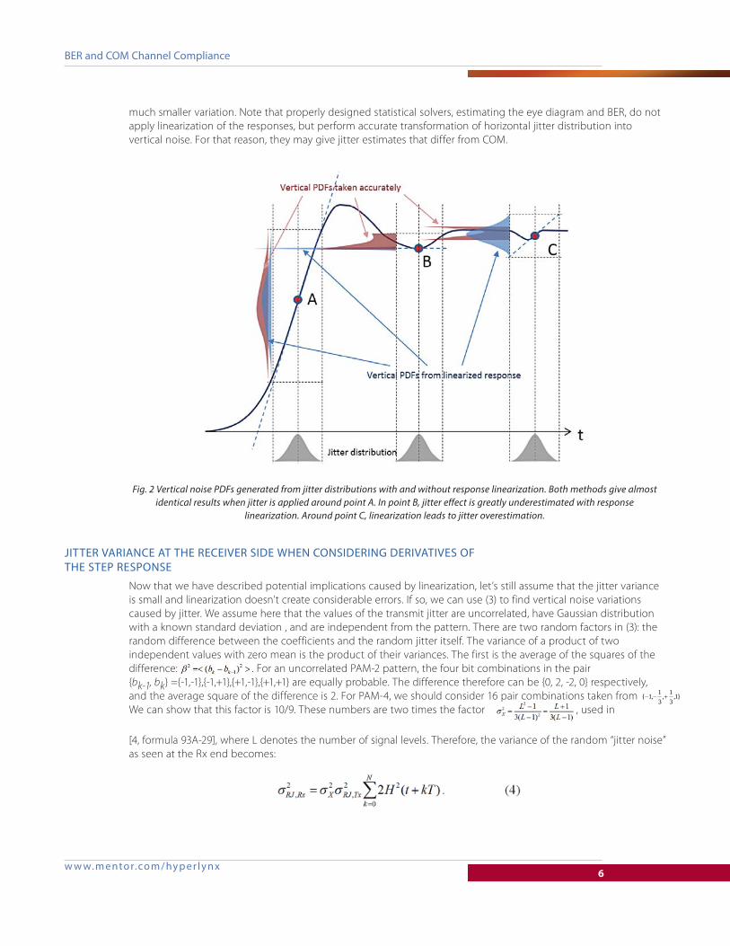
The exact mechanism of how the timing jitter translates into a vertical noise is shown in Fig.2. The gray PDF curves

(probability density functions) are shown at the bottom. We assume that jitter causes a random horizontal

deviation of the sample point, as defined by these PDFs. This deviation translates into a vertical movement of the

sampled value. At every particular location, the vertical distribution depends on the shape of the step response and

jitter PDF. If the response is linearized around the sample point, the resulting noise PDF is similar by shape to the

timing jitter. These PDFs are shown in blue. The accurate transformations result in a set of PDFs which are shaped

differently at every sample location (brown). When the response can be approximated by a straight line (point A),

both approaches give very similar PDFs. At point B, the slope of the curve is zero, therefore the linear

transformation doesn’t produce any vertical noise (i.e., we have a Dirac-impulse PDF), whereas the accurate

transformation shows a considerable vertical variation. In contrast to that, at point C the derivative of the step

response is non-zero, and the linear transformation produces considerable vertical noise. However, since the step

response doesn’t change much in the vicinity of point C, the accurate transformation produces a vertical PDF with



much smaller variation. Note that properly designed statistical solvers, estimating the eye diagram and BER, do not

apply linearization of the responses, but perform accurate transformation of horizontal jitter distribution into

vertical noise. For that reason, they may give jitter estimates that differ from COM.

JITTER VARIANCE AT THE RECEIVER SIDE WHEN CONSIDERING DERIVATIVES OF THE STEP RESPONSE

Now that we have described potential implications caused by linearization, let’s still assume that the jitter variance

is small and linearization doesn’t create considerable errors. If so, we can use (3) to find vertical noise variations

caused by jitter. We assume here that the values of the transmit jitter are uncorrelated, have Gaussian distribution

with a known standard deviation , and are independent from the pattern. There are two random factors in (3): the

random difference between the coefficients and the random jitter itself. The variance of a product of two

independent values with zero mean is the product of their variances. The first is the average of the squares of the

difference: . For an uncorrelated PAM-2 pattern, the four bit combinations in the pair

{bk-1, bk} ={-1,-1},{-1,+1},{+1,-1},{+1,+1} are equally probable. The difference therefore can be {0, 2, -2, 0} respectively,

and the average square of the difference is 2. For PAM-4, we should consider 16 pair combinations taken from

We can show that this factor is 10/9. These numbers are two times the factor , used in

[4, formula 93A-29], where L denotes the number of signal levels. Therefore, the variance of the random “jitter noise”

as seen at the Rx end becomes:

Fig. 2 Vertical noise PDFs generated from jitter distributions with and without response linearization. Both methods give almost identical results when jitter is applied around point A. In point B, jitter effect is greatly underestimated with response

linearization. Around point C, linearization leads to jitter overestimation.

}1,31,

31,1{



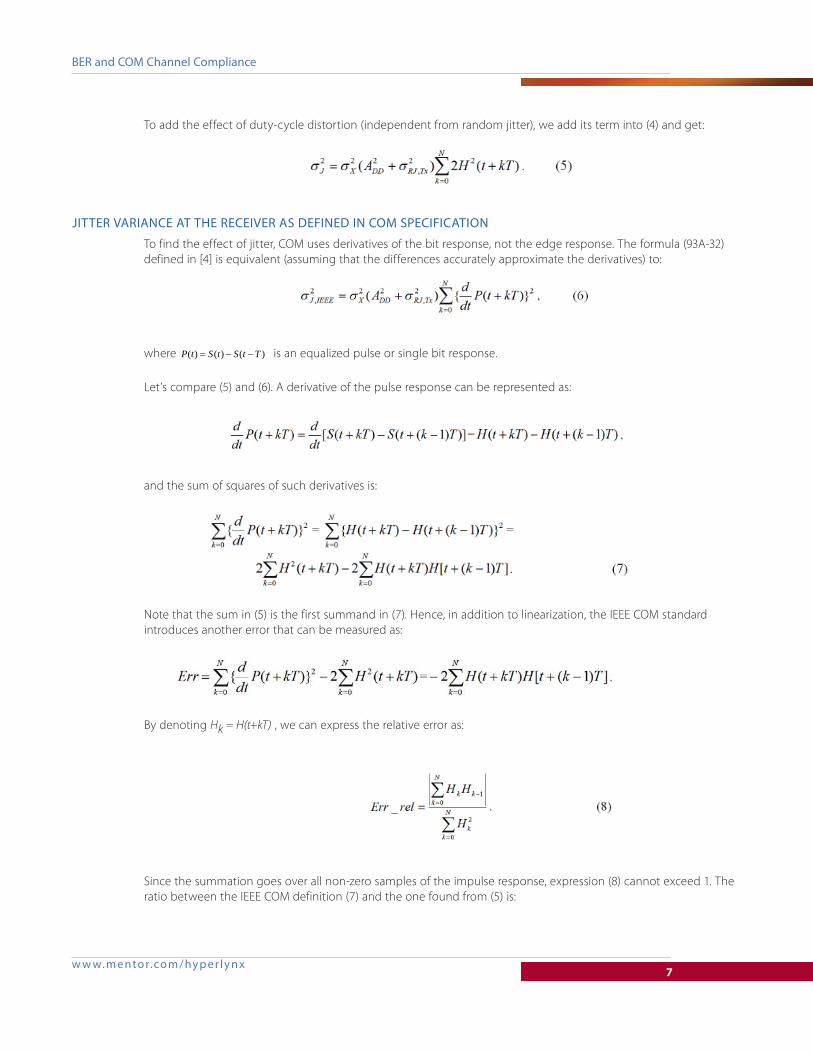
To add the effect of duty-cycle distortion (independent from random jitter), we add its term into (4) and get:

JITTER VARIANCE AT THE RECEIVER AS DEFINED IN COM SPECIFICATION

To find the effect of jitter, COM uses derivatives of the bit response, not the edge response. The formula (93A-32)

defined in [4] is equivalent (assuming that the differences accurately approximate the derivatives) to:

where )()()( TtStStP is an equalized pulse or single bit response.

Let’s compare (5) and (6). A derivative of the pulse response can be represented as:

and the sum of squares of such derivatives is:

Note that the sum in (5) is the first summand in (7). Hence, in addition to linearization, the IEEE COM standard

introduces another error that can be measured as:

By denoting Hk = H(t+kT) , we can express the relative error as:

Since the summation goes over all non-zero samples of the impulse response, expression (8) cannot exceed 1. The

ratio between the IEEE COM definition (7) and the one found from (5) is:



Note that (9) is non-negative but always less than 1. Therefore it appears that COM underestimates contributions

from transmit jitter. Let’s see by how much.

Below, we consider 10GBASE-KR channel, operating at 10.31 Gbps. First, we performed jitter evaluation for a

channel without equalization. Its step response is shown in Fig.3a in red, and pulse response — the difference

between the step response and its delayed copy — in blue. Fig.3b shows the derivatives of the step (red) and pulse

(blue) responses. Note that these are quite different by magnitude around the point where the pulse response

reaches its peak. This alone leads to underestimation of variance in the IEEE COM version by factor 0.64, and with

the additional 2x factor in (5) makes it 0.32, as shown in Fig. 3c. It’s interesting to see how this ratio changes with bit

rate. As we see from Fig.3d, at higher bit rate, the ratio goes further down and reaches 0.17 at 25 Gbps, which is

equivalent by taking only sqrt(0.17)=0.46 of the Gaussian sigma or peak-to-peak sine jitter.

Fig. 3 Non-equalized responses. Formulas (5) and (7) give considerably different estimations. (a) – non-equalized step and pulse responses;

(b) – comparison of the Dirac impulse and derivative of the pulse response; (c) – how the two variance estimates and their ratio change along 1UI. The star shows the chosen sampling location;

(d) the ratio of the two estimates as a function of bit rate.



However, with an equalized response, the plots look different. Equalization modifies the response in such a way

that rising and falling transitions occur “faster”. The correlation coefficients between neighbor samples defining the

sum in the nominator of (8) and (9) gets smaller and the two jitter estimates become closer to each other. Another

explanation is also possible: equalized step and pulse responses become closer to each other by magnidute, as

seen in Fig.4a. Since the pulse response has two distinct slopes, rising and falling, it makes up for the factor “2”

added in the step-response-based jitter evaluation. However, even for the equalized responses we see that the

variance of jitter found from (7) is only 0.8 of the more accurate estimate suggested by (5).

III.

CROSSTALK EVALUATION IN COM AND BERAnother important difference between the COM and BER approaches is how they evaluate the effect of crosstalk.

Both start from forming the single-bit response. This is possible because jitter in the aggressor channels is often

neglected. Crosstalk contribution is evaluated by taking the cursors of the pulse response and considering their

Fig.4 Equalized responses. The difference between jitter estimates is smaller. (a) – step and pulse responses; (b) – comparison of the Dirac impulse and derivative of the pulse response; (c) – how the two

variance estimates change along 1UI; (d) the ratio of the two estimates as a function of bit rate.



magnitudes. The cursors are samples of the response taken with a constant step that equals the bit interval. As we

see from Fig.5, depending on the initial phase within bit interval, we can get different sets of samples. Both COM

and BER take these samples, and for every initial phase (typically, they consider 32 phase values within 1UI) find the

PDF of the random value described by equation:

In (10), the parameter ],0[ T designates initial phase, )(, kxtP are cursors of the pulse response, and bk are

random, statistically independent symbol magnitudes. They could be either }1,1{ for PAM-2 or }1,31,

31,1{

for PAM-4 modulation.

A difference exists in how COM and BER consider initial phases. Accurate BER evaluation assumes that initial phases

of the crosstalk input are random and uniformly distributed within 1UI. For that reason, it finds the averaged PDF of

the crosstalk input by integrating the partial PDFs:

Fig.5 Aggressor’s pulse response. The cursors can be taken with different initial phase, which affects the mean deviation and distribution of the crosstalk noise.



In the COM procedure, we first find the initial phase, for which the variance and standard deviation of the crosstalk

noise is maximal:

N

kkxtP

1

2,max )}(max{ . Then, we continue with the PDF found for this initial phase:

Let’s see how big the effect of this choice on the crosstalk PDF could be. Take, for example, an equalized pulse

response of the aggressor channel, as in Fig.6a. The zoomed portion of the same response around its peak value is

also shown in Fig.6. The two peaks of the standard deviation in Fig.6b are evidently caused by the two prominent

extremes of the pulse response. Note that the standard deviation of the crosstalk noise is a periodic function, with a

period 1UI. The crosstalk PDF is also a periodic function (Fig6c). The contour lines encompass 20 orders of

magnitude; therefore the vertical swing of the PDF is about plus/minus 10 sigma. In Fig.6d, we compare the PDF

considered by COM (red), which is a cross-section taken at ~0.18UI in Fig.6c, and the averaged PDF computed by

formula (11). As we see, the averaged PDF is not Gaussian and has a peak in the middle, caused by considerable

contribution from the portions of the PDFs that have smaller deviation. The peak mean deviation is reflected, too: it

defines how quickly the resulting PDF decreases with the offset. We can show that outside the mid portion, the

accurate PDF is a peak mean-value PDF shifted down.

Fig.6 Single-bit (pulse) response from the aggressor channel: (a), standard deviation of the crosstalk noise versus initial phase

(b), noise PDF as a function of phase (the contours span 20 orders of magnitude) (c), and a comparison between the averaged PDF (blue) and the one selected by COM (red) (d).



If we converted both PDF functions into CDF and find the offsets at 1e-12, we’d get about 6% difference between

the two estimations. At 10-5, the difference is about 10%. Of course, the numbers can vary from case to case, but

the general conclusion is that COM overestimates the effect of crosstalk.

IV. HOW WE COMPARE THE RESULTS FROM COM AND BER SIMULATIONSFinding correlation between COM and BER simulation results isn’t easy. There are some works [6, 7, and 8] that

establish general correlation between BER and COM results, but they don’t compare the computation techniques

and don’t try to put the results side-by-side. We are going to demonstrate a valid comparison technique.

Many simulation tools that compute eye and BER plots can generate or import the step or pulse response of the

victim and aggressor channels. They can also find the optimal equalization parameters or allow the user to set up

them. And, they can also allow adding Tx and Rx jitter and noise. Some simulators of that kind take the responses

found from SPICE-level simulation of the channels together with the buffer models. It is technically difficult to

produce a single bit or step response for a non-linear channel driven by a logical buffer. By definition, both step

and pulse response should be computed starting with zero initial conditions as they describe a single (one-sided)

transition or pulse. Instead, the simulators produce the edge or bit responses, where the states are changing

between “low” and “high” so that the responses have approximately double the magnitude expected for the step

or pulse response.

Fig.7 Measuring signal and noise magnitude on a BER plot: COM report (a), position of the “signal” sample on the eye diagram (b), corresponding BER plot (c), and BER cut-off below 5e-6 to ease measurements.



There are several steps in COM and BER computations which may go differently. If we want to see how the

numbers compare with identical input (most importantly – the same channel responses), it makes sense to take the

responses generated by COM and use them in eye/BER simulation. In our implementation, we can save both pulse

and step responses, equalized and non-equalized, as they were found along with COM evaluation. These responses

can be taken as an input to the eye/BER-computation tool, by considering the 2X difference in magnitude.

Since in BER analysis we reuse the victim’s primary response from COM, the magnitude of the “signal” is the same in

both cases. It is defined by the chosen sample of the equalized pulse response, and can be taken from the COM

report (Fig.7a). On the eye diagram, the signal magnitude can be found somewhere along the vertical cross-section

that corresponds to the largest eye opening, while its vertical position (Y-coordinate) corresponds to the middle of

the top (or bottom) branch of the eye, as in Fig.7b. The corresponding statistical BER plot, where we need to

measure the offset at a specified BER level, could be fuzzy since it spans a wide range of probabilities (Fig.7c). If the

tool allows, it’s convenient to set up the needed threshold and the eliminate BER profile below this level. The cut-

off probability in Fig.7d is 5e-6, half the target detector error ratio, specified by COM for a chosen operation mode.

The reason we take half of the specified level is the different normalization of BER in the eye/BER and COM

procedures. As shown in [5], accurate BER evaluation is described by formula BER = P1P10 + P0P01, where P1 and P0

are the probabilities of transmitting bit ‘1’ or ‘0’ respectively, and P01,P10 evaluate the probability of two possible

errors: reading ‘1’ as ‘0’ or ‘0’ as ‘1’. For a DC balanced signal, P1 = P0 = 0.5 and (1) becomes BER = 0.5(P10 + P01),

making the probability of error at very high or very low threshold equal 0.5. But the COM procedure considers only

one branch of the eye diagram (e.g., the upper), and assumes that the corresponding CDF is normalized so that its

full integral equals 1.

From Fig.7d, we find that the eye opening at the specified BER level is 0.0203. Hence, the noise magnitude is:

A*ni = A*s – A*eye =0.0384-0.0203=0.0181. From here, we can evaluate COM* = 20log10(A*s /A*ni) =6.53 dB. This value

is close to what we get from the COM report (6.36dB). The difference can be explained by the way we consider

jitter and crosstalk, and some imperfectness of measurements we performed on the eye and BER plots, for

example, caused by a discreteness of the mesh.

V. EXPERIMENTAL COM VS IMPROVED COM COMPARISONTo evaluate the error introduced by the simplifications made in the COM method in regards to jitter and crosstalk

contributions, a set of eight pre-layout schematics that mimic the behavior of a 100GBASE-KR4 electrical backplane

system was created. All of these schematics implement, as shown in Fig. 8, a variation of the same topology

containing the backplane, connectors, and two daughter-cards attached at each end. The two connectors support

25-Gbps data rates. The wide bus topology includes five coupled differential pairs, with a victim pair in the center

and four aggressors (two on each side of the victim). The two near-end aggressors (NEXT) have opposite signaling

flow compared to the victim pair, while the two far end aggressors (FEXT) have the same signaling flow as the

victim pair. The total length of the channel is 47cm (19 inches), with 40 cm (16 inches) on the backplane and 7 cm (3

inches) on each of the daughter-cards. The backplane stackup contains 24 layers: 14 signal layers (2 microstrip and

12 edge-coupled striplines) and 10 power/ground layers. The daughter-cards’ stackup is similar to the backplane

stack-up, but is thinner and has only 18 layers: 10 signal layers (2 microstrip and 8 edge-coupled stripline) and 8

power/ground layers. The main routing on the backplane and daughter-cards is stripline with short microstrip

connector breakouts (0.5 inch on each side of the connector). The geometry of the traces was chosen to meet the

50 ohm single-ended and respectively 100-ohm differential impedance, or to be as close as possible to them. The

differential vias were also optimized for 100-ohm differential impedance, except in the case of the first

configuration where intentional stubs lowered the impedance of the backplane differential vias down to ~64 ohm.



The main elements that differentiate the eight configurations are:

1. Configuration 1 – higher-loss material (FR406 with Er = 3.93 and Loss Tangent = 0.0167), reflections due to long

via stubs, and a high level of crosstalk. The main routing on the backplane was done in layer 3 and the vias were

not backdrilled, leaving long via stubs (layer 3 to layer 24). The inter-pair spacing was 2.5 times the dielectric height

(10 mils).

2. Configuration 2 – higher-loss material, reflections due to long via stubs were suppressed, and high level of

crosstalk. The second configuration inherits the material properties and inter-pair spacing from the previous

configuration (FR406 and 10 mils pair-to-pair spacing). The main routing on the backplane was moved from layer 3

to layer 22, thus the via stubs are much shorter. The inter-pair spacing was kept the same as in the first

configuration.

3. Configuration 3 – low-loss dielectric material and high crosstalk. This version of the system topology was

derived from the second configuration by replacing the FR406 board material with Megtron 6 (Er = 3.71, Loss

Tangent = 0.002).

4. Configurations 4 to 8 – low-loss material and lower crosstalk. Those configurations are improved versions of

configuration 3 from the crosstalk perspective. The pair-to-pair spacing was incrementally increased from 2.5 times

the dielectric height (10 mils) up to 5 times the dielectric height (20 mils).

Fig. 8 Simulated topology

Fig.9 Differential via structures: configuration 1 (a), all the other configurations (b)



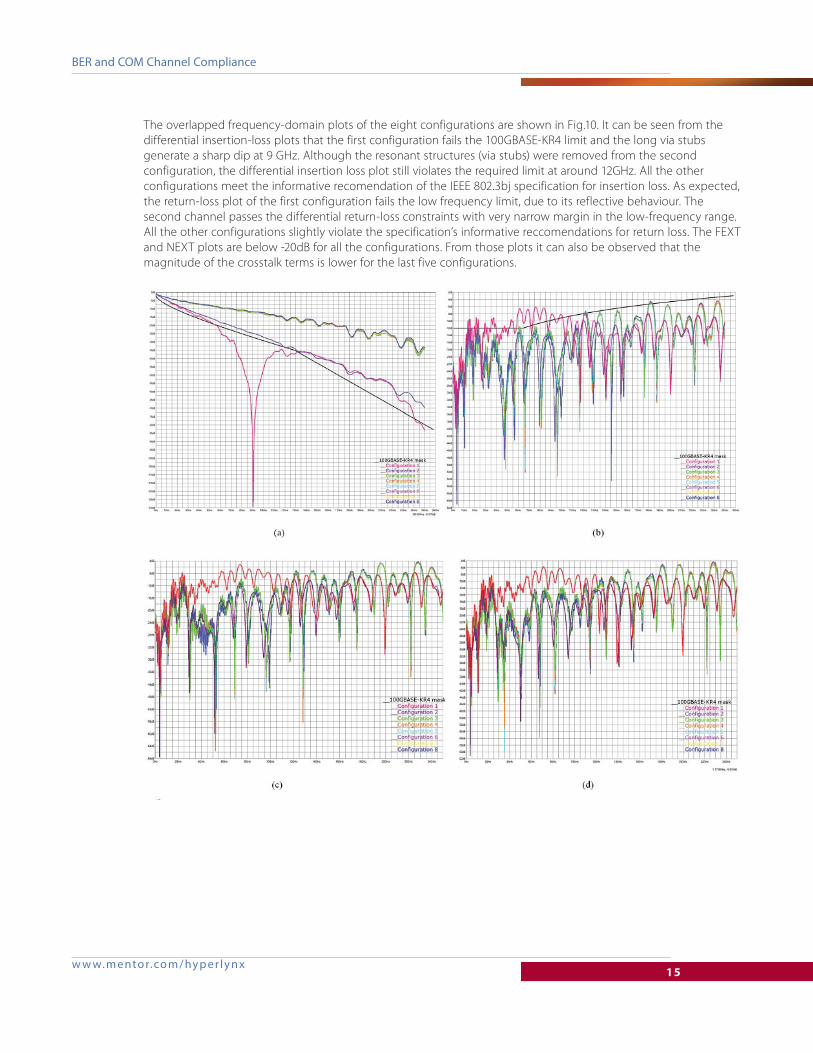
The overlapped frequency-domain plots of the eight configurations are shown in Fig.10. It can be seen from the

differential insertion-loss plots that the first configuration fails the 100GBASE-KR4 limit and the long via stubs

generate a sharp dip at 9 GHz. Although the resonant structures (via stubs) were removed from the second

configuration, the differential insertion loss plot still violates the required limit at around 12GHz. All the other

configurations meet the informative recomendation of the IEEE 802.3bj specification for insertion loss. As expected,

the return-loss plot of the first configuration fails the low frequency limit, due to its reflective behaviour. The

second channel passes the differential return-loss constraints with very narrow margin in the low-frequency range.

All the other configurations slightly violate the specification’s informative reccomendations for return loss. The FEXT

and NEXT plots are below -20dB for all the configurations. From those plots it can also be observed that the

magnitude of the crosstalk terms is lower for the last five configurations.



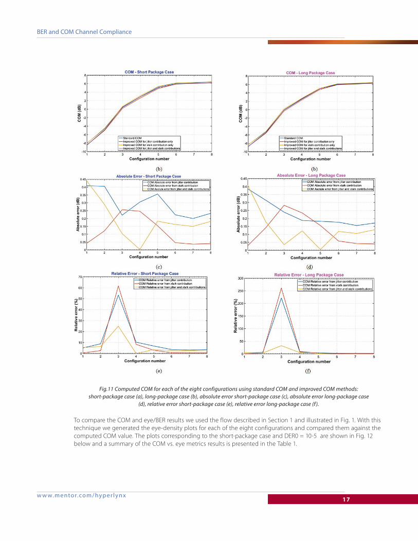
For each of those configurations, two channel operation margins were calculated: one using the method described

in the IEEE 802.3bj standard and another one using the improved algorithm proposed in this paper. The computed

COM values are ranging from -8.7 dB to 6.43 dB with a minimum attained in the case of configuration 1 and a

maximum in the configuration 8 case. COM is way below the 3dB threshold for the first three configurations, clearly

indicating that those are failing channels. The fourth configuration passes the 3dB threshold with almost no margin.

The last four configurations pass the specification limits with good margins. The first two plots, (a) and (b), shown in

Fig 11, describe COM variation versus configuration number for the two package cases (short and long). The next

two plots, (c) and (d) from the same figure, indicate the absolute error between the two methods for COM

computation. In the last two plots, (e) and (f), the comparative accuracy of these methods is quantified in terms of

their relative errors. The first four plots reveal that the maximum absolute error for all the configurations under

consideration is 0.44 dB and it occurs in the short package case for the first configuration.

From the last two plots it can be seen that the relative error between the two methods of COM computation can

be as high as 24% in the short package case and 32% in the long package case. Those maximum values correspond

to configuration 3 for which the computed COM values are near 0 dB. The relative error diminishes as COM goes

below or above 0 dB.

From these plots, and especially from Fig.11 a,b, we see that the modified version of COM procedure shows more

effect from jitter, although the results are slightly less sensitive to crosstalk. This observation agrees with

estimations made in Sections II and III.

Fig. 10 Overlapped frequency-domain characteristics of the eight configurations: differential insertion loss of the victim pairs plotted against the 100GBASE-KR4 limit. (a), differential return loss of the victim pairs plotted against the 100GBASE-KR4 limit

(b), aggressor 1 NEXT (c), aggressor 2 (FEXT) (d), aggressor 3 (NEXT) (e), and aggressor 4 (FEXT) (f ).



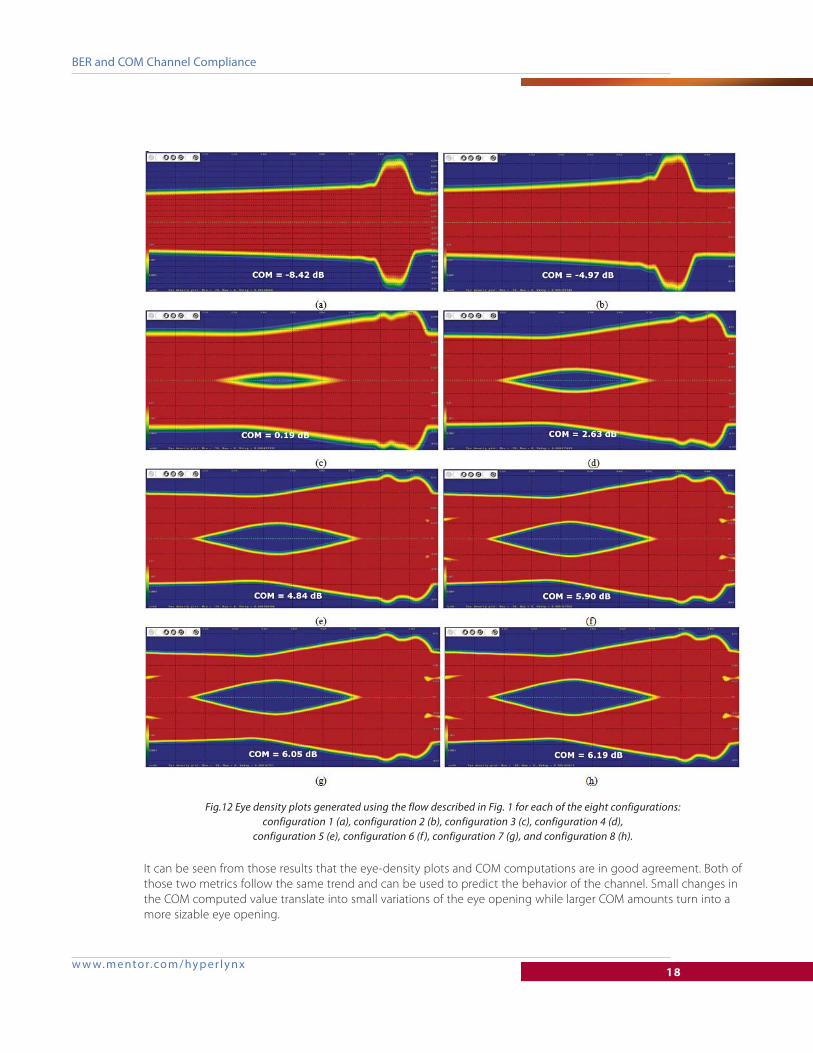
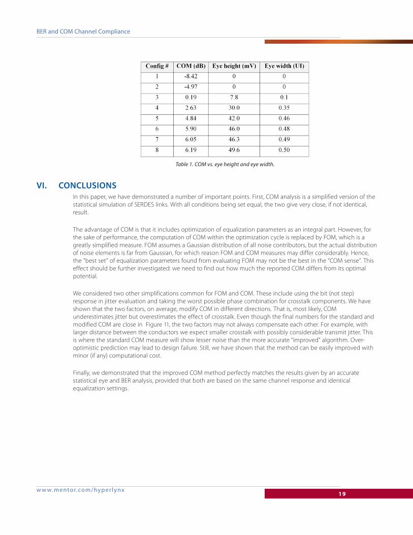
To compare the COM and eye/BER results we used the flow described in Section 1 and illustrated in Fig. 1. With this

technique we generated the eye-density plots for each of the eight configurations and compared them against the

computed COM value. The plots corresponding to the short-package case and DER0 = 10-5 are shown in Fig. 12

below and a summary of the COM vs. eye metrics results is presented in the Table 1.

Fig.11 Computed COM for each of the eight configurations using standard COM and improved COM methods: short-package case (a), long-package case (b), absolute error short-package case (c), absolute error long-package case

(d), relative error short-package case (e), relative error long-package case (f ).



It can be seen from those results that the eye-density plots and COM computations are in good agreement. Both of

those two metrics follow the same trend and can be used to predict the behavior of the channel. Small changes in

the COM computed value translate into small variations of the eye opening while larger COM amounts turn into a

more sizable eye opening.

Fig.12 Eye density plots generated using the flow described in Fig. 1 for each of the eight configurations: configuration 1 (a), configuration 2 (b), configuration 3 (c), configuration 4 (d),

configuration 5 (e), configuration 6 (f ), configuration 7 (g), and configuration 8 (h).



VI. CONCLUSIONSIn this paper, we have demonstrated a number of important points. First, COM analysis is a simplified version of the

statistical simulation of SERDES links. With all conditions being set equal, the two give very close, if not identical,

result.

The advantage of COM is that it includes optimization of equalization parameters as an integral part. However, for

the sake of performance, the computation of COM within the optimization cycle is replaced by FOM, which is a

greatly simplified measure. FOM assumes a Gaussian distribution of all noise contributors, but the actual distribution

of noise elements is far from Gaussian, for which reason FOM and COM measures may differ considerably. Hence,

the “best set” of equalization parameters found from evaluating FOM may not be the best in the “COM sense”. This

effect should be further investigated: we need to find out how much the reported COM differs from its optimal

potential.

We considered two other simplifications common for FOM and COM. These include using the bit (not step)

response in jitter evaluation and taking the worst possible phase combination for crosstalk components. We have

shown that the two factors, on average, modify COM in different directions. That is, most likely, COM

underestimates jitter but overestimates the effect of crosstalk. Even though the final numbers for the standard and

modified COM are close in Figure 11, the two factors may not always compensate each other. For example, with

larger distance between the conductors we expect smaller crosstalk with possibly considerable transmit jitter. This

is where the standard COM measure will show lesser noise than the more accurate “improved” algorithm. Over-

optimistic prediction may lead to design failure. Still, we have shown that the method can be easily improved with

minor (if any) computational cost.

Finally, we demonstrated that the improved COM method perfectly matches the results given by an accurate

statistical eye and BER analysis, provided that both are based on the same channel response and identical

equalization settings.

Table 1. COM vs. eye height and eye width.

MISC2363-wMF 2-16

©2016 Mentor Graphics Corporation, all rights reserved. This document contains information that is proprietary to Mentor Graphics Corporation and may be duplicated in whole or in part by the original recipient for internal business purposes only, provided that this entire notice appears in all copies. In accepting this document, the recipient agrees to make every reasonable effort to prevent unauthorized use of this information. All trademarks mentioned in this document are the trademarks of their respective owners.

F o r t h e l a t e s t p r o d u c t i n f o r m a t i o n , w w w . m e n t o r . c o m / h y p e r l y n x


REFERENCES1. V. Stojanovic, M. Horiwitz, Modeling and analysis of high-speed links, Proc. IEEE Custom Integrated Circuit

Conf., pp. 589–594, Sept 2003

2. J. Caroselly, C. Liu, An analytic system model for high-speed interconnects and its application to the

specification of signaling and equalization architectures for 10Gbps backplane communications, DesignCon,

2006

3. M. Tsuk, D. Dvorscsak, C.S. Ong, and J. White, An electrical-level superimposed-edge approach to statistical

serial link simulation, IEEE/ACM International Conf. on Computer-aided Design Digest of Technical Papers, pp.

718–724, 2009

4. IEEE Std. 802.3bj-2014 (Amendment to IEEE Std. 802.3-2012), Annex 93A.1, Channel Operating Margin

5. V. Dmitriev-Zdorov, M. Miller, C. Ferry, The Jitter-Noise Duality and Anatomy of an Eye Diagram, DesignCon

2014

6. M. Rowlands, I. Park, D. Correia, What Makes a Good Channel? COM vs. BER Metrics, DesignCon 2015

7. X. Dong, M. Mo, F. Rao, W. Jin., G. Zhang, Relating COM to Familiar S-Parameter Parametric to Assist 25Gbps

System Design, , DesignCon 2014

8. R. Mellitz, A. Ran, M. Peng Li, V. Ragavassamy, Channel Operating Margin (COM): Evolution of Channel

Specifications for 25 Gbps and Beyond, DesignCon 2013

9. M. Brown, M. Dudek, A. Healey, L. B. Artsi, R. Mellitz, C. Moore, A. Ran, P. Zivny, The state of IEEE 802.3bj 100

Gb/s Backplane Ethernet, DesignCon 2014

10. B. Gore, R. Mellitz, An Exercise in Applying Channel Operating Margin (COM) for 10GBASE-KR Channel Design,

IEEE International Symposium on Electromagnetic Compatibility (EMC) 2014

ber- and com-way of channel- compliance evaluation

Technology