1

Lifshitz Gravity and Lifshitz Holography

Petr Horava

Berkeley Center for Theoretical Physics

lecture in the Physics 234B course

BCTP, UC Berkeley

April 2013

1

Lifshitz Gravity and Lifshitz Holography

Petr Horava

Berkeley Center for Theoretical Physics

lecture in the Physics 234B course

BCTP, UC Berkeley

April 2013

2

Outline

I. Review of quantum gravity with anisotropic scalinganisotropic Weyl symmetries & anomalies

detailed balance

II. Lifshitz holographyLifshitz spacetimes

anisotropic conformal infinity

IIa. Lifshitz holography in relativistic gravityholographic renormalization, counterterms

anisotropic Weyl anomalies in detailed balance

detailed balance from recursions among holographic counterterms

IIb. Lifshitz holography in Lifshitz gravityLifshitz spacetime as a vacuum solution

general form of anisotropic Weyl anomalies with examples

general holographic Weyl anomalies from Lifshitz gravity

III. Black holes & Conclusions

3

Some references

initial papers on gravity with anisotropic scaling:

. . ., arXiv:0812.4287, arXiv:0901.3775, . . .

brief recent(ish) review:

arXiv:1101.1081 (GR 19 Proceedings).

focus of this talk:

work with Tom Griffin and Charles Melby-Thompsonin arXiv:1112.5660, 1211.4872, 1301.nnnn

work with Tom Griffin and Omid Saremiin arXiv:to appear very soon

4

I.Review: Gravity with anisotropic scaling

5

Gravity with anisotropic scaling(also known as Horava-Lifshitz gravity)

Field theory with anisotropic scaling (x = xi, i = 1, . . . D):

x→ λx, t→ λzt.

z: dynamical critical exponent – characteristic of RG fixed point.

Many interesting examples: z = 1, 2, . . ., n, . . .fractions: 3/2 (KPZ surface growth in D = 1), . . ., 1/n, . . .families with z varying continuously . . .

Condensed matter, dynamical critical phenomena, quantumcritical systems, . . .

Goal: Extend to gravity, with propagating gravitons, formulatedas a quantum field theory of the metric.

6

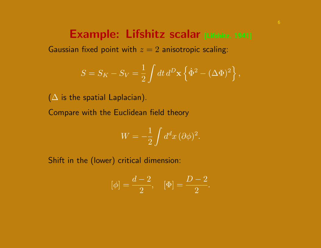
Example: Lifshitz scalar [Lifshitz, 1941]

Gaussian fixed point with z = 2 anisotropic scaling:

S = SK − SV =12

∫dt dDx

Φ2 − (∆Φ)2

,

(∆ is the spatial Laplacian).

Compare with the Euclidean field theory

W = −12

∫ddx (∂φ)2.

Shift in the (lower) critical dimension:

[φ] =d− 2

2, [Φ] =

D − 22

.

7

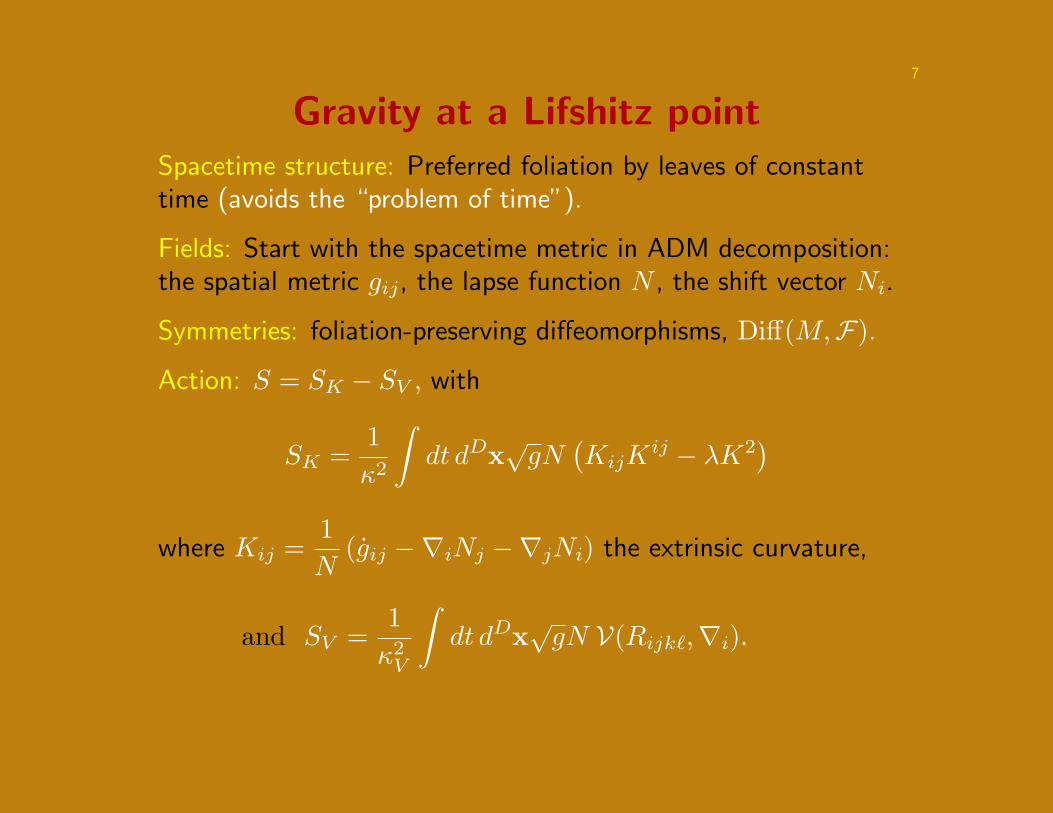
Gravity at a Lifshitz pointSpacetime structure: Preferred foliation by leaves of constanttime (avoids the “problem of time”).

Fields: Start with the spacetime metric in ADM decomposition:the spatial metric gij, the lapse function N , the shift vector Ni.

Symmetries: foliation-preserving diffeomorphisms, Diff(M,F).

Action: S = SK − SV , with

SK =1κ2

∫dt dDx

√gN

(KijK

ij − λK2)

where Kij =1N

(gij −∇iNj −∇jNi) the extrinsic curvature,

and SV =1κ2V

∫dt dDx

√gN V(Rijk`,∇i).

8

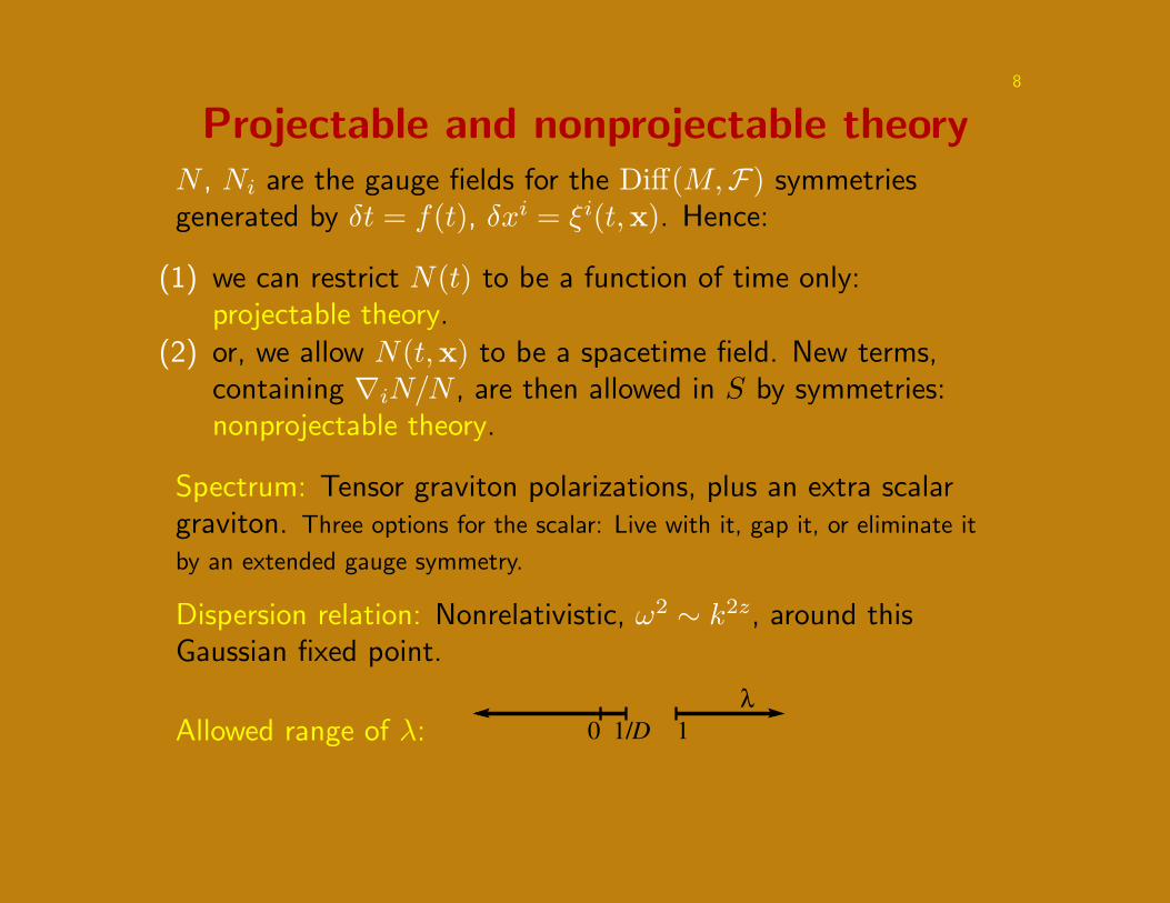
Projectable and nonprojectable theoryN , Ni are the gauge fields for the Diff(M,F) symmetriesgenerated by δt = f(t), δxi = ξi(t,x). Hence:

(1) we can restrict N(t) to be a function of time only:projectable theory.

(2) or, we allow N(t,x) to be a spacetime field. New terms,containing ∇iN/N , are then allowed in S by symmetries:nonprojectable theory.

Spectrum: Tensor graviton polarizations, plus an extra scalargraviton. Three options for the scalar: Live with it, gap it, or eliminate it

by an extended gauge symmetry.

Dispersion relation: Nonrelativistic, ω2 ∼ k2z, around thisGaussian fixed point.

Allowed range of λ: 0 11/D

λ

9

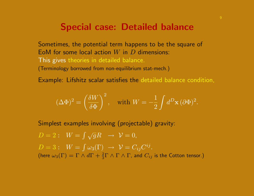
Special case: Detailed balance

Sometimes, the potential term happens to be the square ofEoM for some local action W in D dimensions:This gives theories in detailed balance.(Terminology borrowed from non-equilibrium stat-mech.)

Example: Lifshitz scalar satisfies the detailed balance condition,

(∆Φ)2 =(δW

δΦ

)2

, with W = −12

∫dDx (∂Φ)2.

Simplest examples involving (projectable) gravity:

D = 2 : W =∫ √

gR → V = 0,

D = 3 : W =∫ω3(Γ) → V = CijC

ij.(here ω3(Γ) = Γ ∧ dΓ + 2

3Γ ∧ Γ ∧ Γ, and Cij is the Cotton tensor.)

10

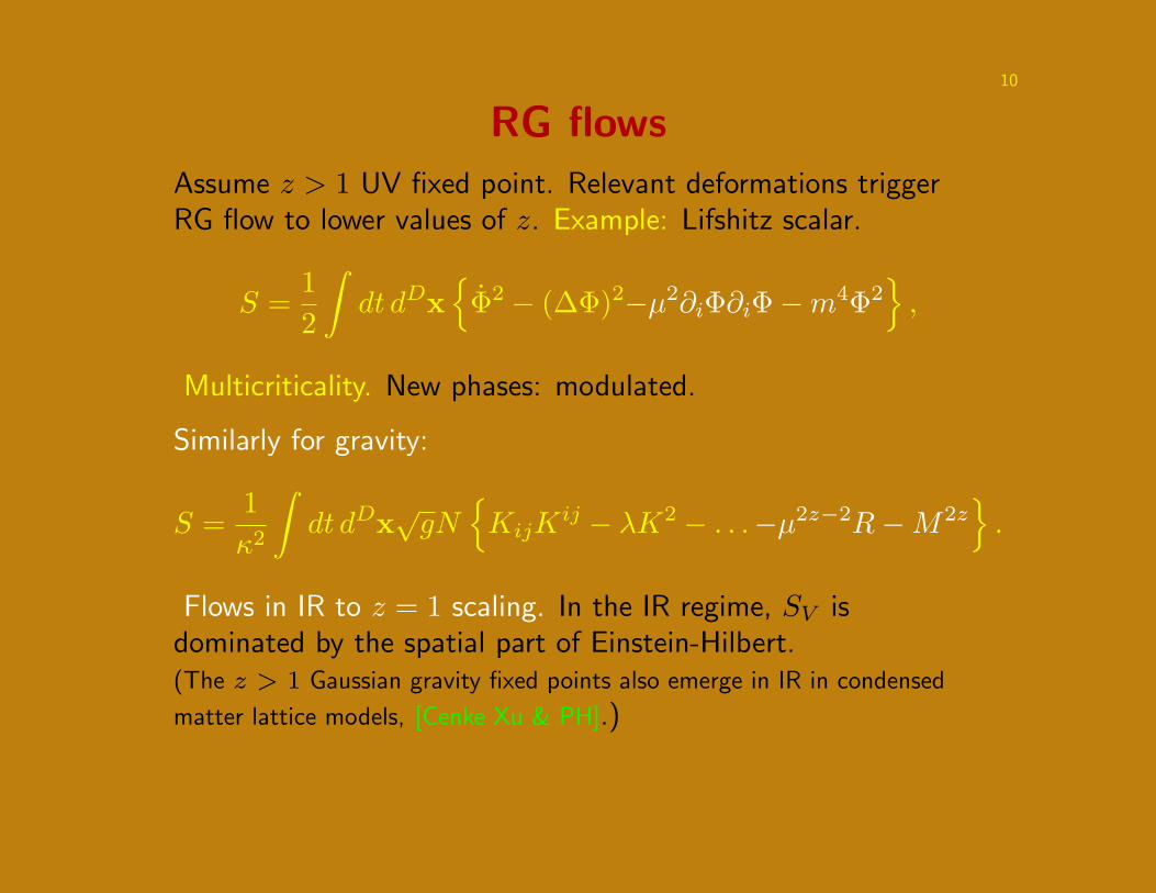
RG flows

Assume z > 1 UV fixed point. Relevant deformations triggerRG flow to lower values of z. Example: Lifshitz scalar.

S =12

∫dt dDx

Φ2 − (∆Φ)2−µ2∂iΦ∂iΦ−m4Φ2

,

Multicriticality. New phases: modulated.

Similarly for gravity:

S =1κ2

∫dt dDx

√gN

KijK

ij − λK2 − . . .−µ2z−2R−M2z.

Flows in IR to z = 1 scaling. In the IR regime, SV isdominated by the spatial part of Einstein-Hilbert.(The z > 1 Gaussian gravity fixed points also emerge in IR in condensed

matter lattice models, [Cenke Xu & PH].)

11

Relevant deformations, RG flows, phasesThe Lifshitz scalar can be deformed by relevant terms:

S =12

∫dt dDx

φ2 − (∆φ)2−µ2∂iφ∂iφ+m4φ2 − φ4

The undeformed z = 2 theory describes a tricritical point,connecting three phases – disordered, ordered, spatiallymodulated (“striped”) [A. Michelson, 1976]:

12

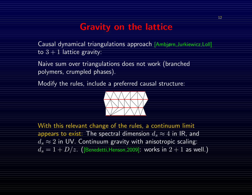
Gravity on the lattice

Causal dynamical triangulations approach [Ambjørn,Jurkiewicz,Loll]

to 3 + 1 lattice gravity:

Naive sum over triangulations does not work (branchedpolymers, crumpled phases).

Modify the rules, include a preferred causal structure:

With this relevant change of the rules, a continuum limitappears to exist: The spectral dimension ds ≈ 4 in IR, andds ≈ 2 in UV. Continuum gravity with anisotropic scaling:ds = 1 +D/z. ([Benedetti,Henson,2009]: works in 2 + 1 as well.)

13

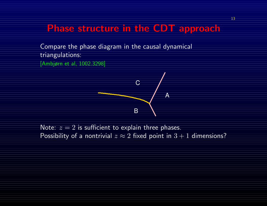
Phase structure in the CDT approach

Compare the phase diagram in the causal dynamicaltriangulations:[Ambjørn et al, 1002.3298]

C

B

A

Note: z = 2 is sufficient to explain three phases.Possibility of a nontrivial z ≈ 2 fixed point in 3 + 1 dimensions?

14

RG flows in gravity: z = 1 in IR

Theories with z > 1 represent candidates for the UV description.Under relevant deformations, the theory will flow in the IR.Relevant terms in the potential:

∆SV =∫dt dDx

√gN

. . .+µ2(R− 2Λ)

.

the dispersion relation changes in IR to ω2 ∼ k2 + . . .the IR speed of light is given by a combination of the couplingsµ2 combines with κ, . . . to give an effective GN .

Sign of k2 in dispersion relation is opposite for the scalar andthe tensor modes! Can we classify the phases of gravity? Cangravity be in a modulated phase?

15

Spatially homogeneous isotropic phasesof gravity

vglue-.5in Examples of phases of gravity with k = 1: a deSitter-like phase, an oscillating cosmology (=“temporallymodulated” phase); the Einstein static universe appears at thephase transition line, where the theory satisfies detailed balance.

Cosmology: [Kiritsis et al, Brandenberger et al, Lust et al, many others]

16

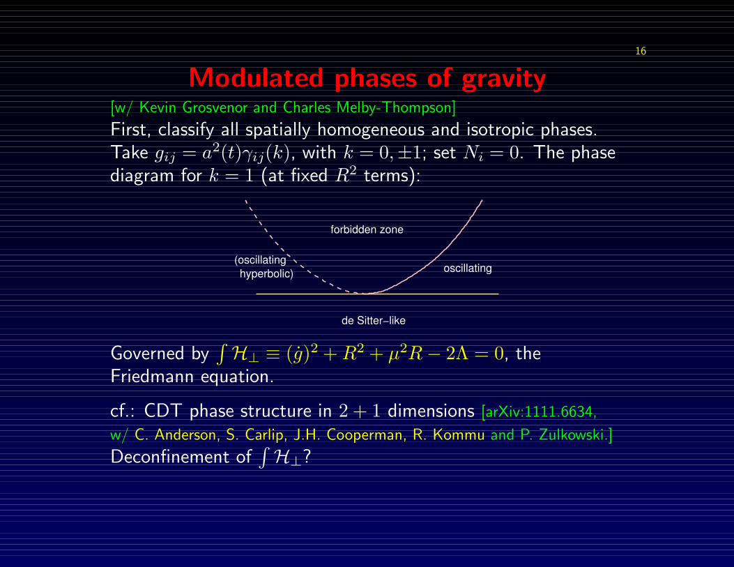
Modulated phases of gravity[w/ Kevin Grosvenor and Charles Melby-Thompson]

First, classify all spatially homogeneous and isotropic phases.Take gij = a2(t)γij(k), with k = 0,±1; set Ni = 0. The phasediagram for k = 1 (at fixed R2 terms):

forbidden zone

oscillating(oscillating

hyperbolic)

de Sitter−like

Governed by∫H⊥ ≡ (g)2 +R2 + µ2R− 2Λ = 0, the

Friedmann equation.

16

Modulated phases of gravity[w/ Kevin Grosvenor and Charles Melby-Thompson]

First, classify all spatially homogeneous and isotropic phases.Take gij = a2(t)γij(k), with k = 0,±1; set Ni = 0. The phasediagram for k = 1 (at fixed R2 terms):

forbidden zone

oscillating(oscillating

hyperbolic)

de Sitter−like

Governed by∫H⊥ ≡ (g)2 +R2 + µ2R− 2Λ = 0, the

Friedmann equation.

cf.: CDT phase structure in 2 + 1 dimensions [arXiv:1111.6634,

w/ C. Anderson, S. Carlip, J.H. Cooperman, R. Kommu and P. Zulkowski.]

Deconfinement of∫H⊥?

17

Anisotropic Weyl symmetries

Using a spacetime-dependent scaling factor Ω(t,x) = eω(t,x),define

gij → Ω2gij, Ni → Ω2Ni, N → ΩzN.

Such anisotropic Weyl transformations are compatible withfoliation-preserving diffeos:

Weylz(M,F) ⊂×Diff(M,F).

Indeed, [δω, δf,ξi] = δfω+ξi∂iω.

This provides the appropriate generalization of local “conformaltransformations” to foliated spacetimes with anisotropic scaling.

Often, it is sufficient to have the preferred foliation and the anisotropic Weyl

transformations defined only asymptotically, “near infinity.”

18

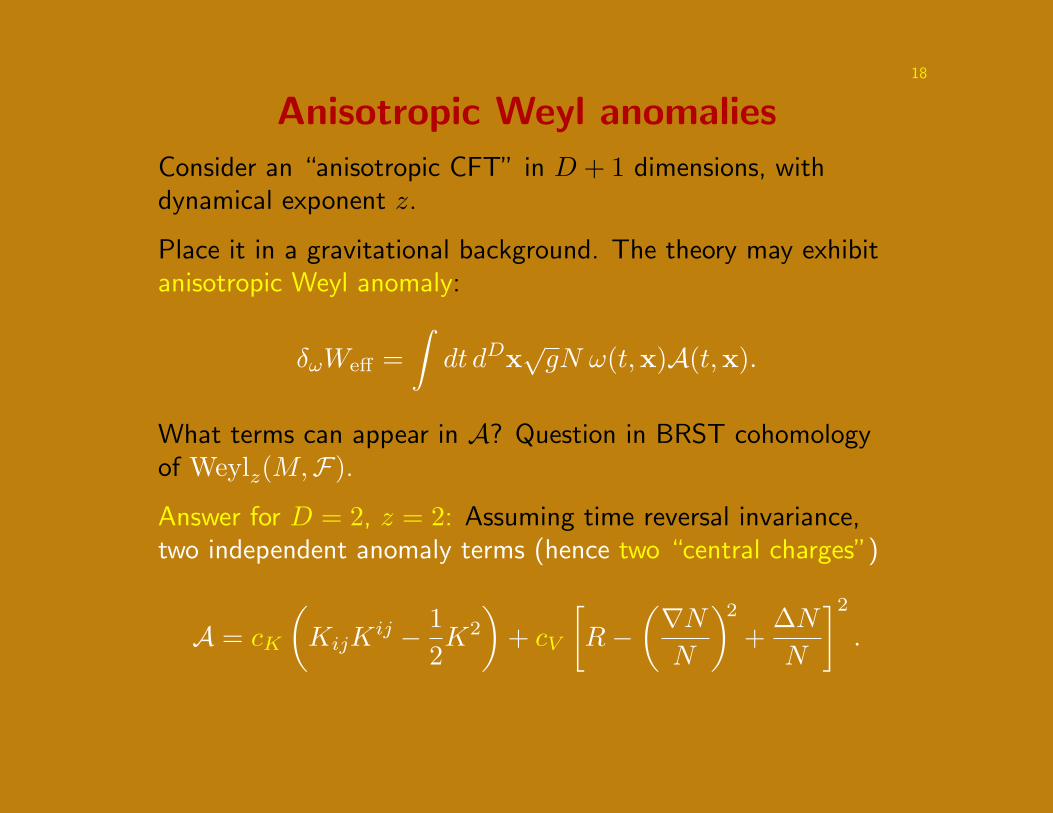
Anisotropic Weyl anomalies

Consider an “anisotropic CFT” in D + 1 dimensions, withdynamical exponent z.

Place it in a gravitational background. The theory may exhibitanisotropic Weyl anomaly:

δωWeff =∫dt dDx

√gN ω(t,x)A(t,x).

What terms can appear in A? Question in BRST cohomologyof Weylz(M,F).

Answer for D = 2, z = 2: Assuming time reversal invariance,two independent anomaly terms (hence two “central charges”)

A = cK

(KijK

ij − 12K2

)+ cV

[R−

(∇NN

)2

+∆NN

]2

.

19

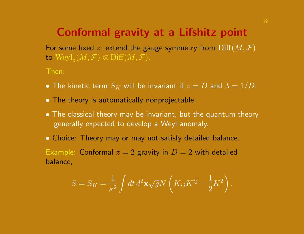
Conformal gravity at a Lifshitz pointFor some fixed z, extend the gauge symmetry from Diff(M,F)to Weylz(M,F) ⊂×Diff(M,F).

Then:

• The kinetic term SK will be invariant if z = D and λ = 1/D.

• The theory is automatically nonprojectable.

• The classical theory may be invariant, but the quantum theorygenerally expected to develop a Weyl anomaly.

• Choice: Theory may or may not satisfy detailed balance.

Example: Conformal z = 2 gravity in D = 2 with detailedbalance,

S = SK =1κ2

∫dt d2x

√gN

(KijK

ij − 12K2

).

20

II.Lifshitz holography

21

Lifshitz holographyAdS:

ds2 = r2(−dt2 + dx2) + dr2/r2r

Lifshitz:

ds2 = −r2zdt2 + r2dx2 + dr2/r2r

Focus of this talk:The role of HL gravity for Lifshitz spacetime.

22

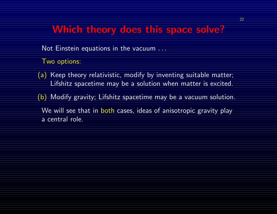
Which theory does this space solve?

Not Einstein equations in the vacuum . . .

Two options:

(a) Keep theory relativistic, modify by inventing suitable matter;Lifshitz spacetime may be a solution when matter is excited.

(b) Modify gravity; Lifshitz spacetime may be a vacuum solution.

We will see that in both cases, ideas of anisotropic gravity playa central role.

23

IIa.Lifshitz holography in relativistic gravity

24

Relativistic holography for Lifshitz space

Various matter sources possible, one of the simplest/mostpopular is a massive vector: [Taylor]

S =1

16πGN

∫dt dDx dr

√−G(R−2Λ)+

18πGN

∫dt dDx

√−gK

− 14

∫dt dDx dr

√−G(FµνFµν + 2m2AµA

µ).

To get Lifshitz with given z as solution, one must take

Λ =12[z2 + (D − 1)z +D2

], m2 = Dz, 〈At〉 =

2(z − 1)z

.

Also, various string/M-theory embeddings now exist.

[Balasubramanian,Narayan; Gauntlett et al; . . . ]

25

Anisotropic conformal infinityEven if we embed Lifshitz space into relativistic gravity withmatter, we need anisotropic scaling to define properly theasymptotic structure near “infinity”.

Conformal infinity [Penrose]: Rescale the bulk metric on M

gµν → gµν ≡ Ω(t,x, r)gµν,

so that gµν now extends “past infinity” of M. Then take M.For Lifshitz spacetimes with z > 1: Conformal infinity is a line!(This contradicts holographic expectations).

Anisotropic conformal infinity [PH & C. Melby-Thompson, 2009]:For asymptotically foliated spacetimes, use anisotropic Weyltransformations instead. Anisotropic conformal infinity ofLifshitz spacetime is of codimension one, with a preferrednonrelativistic foliation. (As expected from holography.)

26

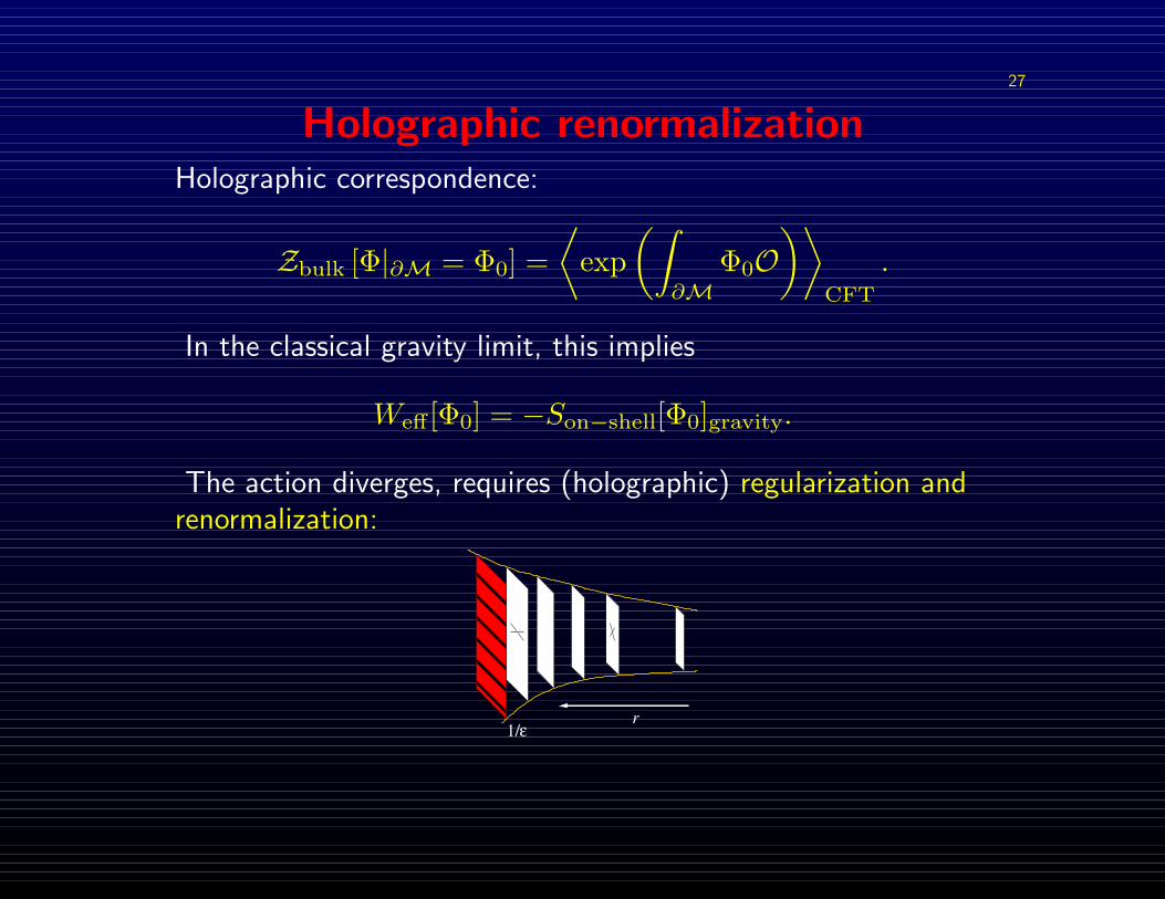
Holographic renormalizationHolographic correspondence:

Zbulk [Φ|∂M = Φ0] =⟨

exp(∫

∂MΦ0O

)⟩CFT

.

In the classical gravity limit, this implies

Weff[Φ0] = −Son−shell[Φ0]gravity.

The action diverges, requires (holographic) regularization andrenormalization:

r

8

27

Holographic renormalizationHolographic correspondence:

Zbulk [Φ|∂M = Φ0] =⟨

exp(∫

∂MΦ0O

)⟩CFT

.

In the classical gravity limit, this implies

Weff[Φ0] = −Son−shell[Φ0]gravity.

The action diverges, requires (holographic) regularization andrenormalization:

r

1/ε

28

Counterterms: Hamilton-Jacobi theory[de Boer, Verlinde, Verlinde; Skenderis et al; Ross & Saremi; . . .]

On-shell action S[gij, Ni, N ; . . .], as a functional of boundaryfields, satisfies HJ equation in radial evolution.

In gravity, this means Hr(παβ =

δS

δgαβ

)= 0

(plus supermomentum constraints).

Parametrize S[gij, Ni, N ] =1

16πGN

∫dt dDx

√gN L.

Note: L is divergent, expand asymptotically as

L = . . .+L(4)

ε4+L(2)

ε2+ L(0)log ε+ L(0) +O(ε2).

Plug into HJ equation, which gives a recursive relation amongcounterterms.

29

Counterterms for z = 2 in D = 2:Conformal Lifshitz gravity

Holographic recursion relations for counterterms can be solvedfor general D and z, at least in principle.

In the first nontrivial conformal case, D = 2 and z = 2, theygive:

L(4) = 6, L(2) =12R+

14

(∇NN

)2

, L(0) = KijKij − 1

2K2.

The recursion relations imply δDL(0) ∼ L(0).Since L(0) is the renormalized action, and δD (=the radialevolution operator) is the anisotropic Weyl rescaling,L(0) gives the anisotropic Weyl anomaly.This anomaly takes the form of z = 2 conformal Lifshitz gravityaction in detailed balance, at the anisotropic boundary.

30

Holographic anomaly in detailed balanceNote that of the two possible central charges, only cK isgenerated in this holographic theory.What distinguishes cK from cV ? The cK anomaly satisfies thedetailed balance condition.

This was further verified for bulk gravity coupled to scalars XI.In addition to the kinetic piece,

1κ2

∫dt d2x

√gN

(KijK

ij − 12K2

)+

12

∫dt d2x

√g

N

(XI −N i∂iX

I)2

,

the anomaly now develops also a potential part,∫dt d2x

√gN

(∆XI)2 +

κ2

2Tij(X)T ij(X)

.

This is in detailed balance, with W = 12

∫d2x√g∂iX

I∂iXI.

31

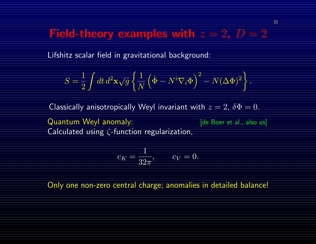
Field-theory examples with z = 2, D = 2

Lifshitz scalar field in gravitational background:

S =12

∫dt d2x

√g

1N

(Φ−N i∇iΦ

)2

−N(∆Φ)2

.

Classically anisotropically Weyl invariant with z = 2, δΦ = 0.

Quantum Weyl anomaly: [de Boer et al., also us]

Calculated using ζ-function regularization,

cK =1

32π, cV = 0.

Only one non-zero central charge; anomalies in detailed balance!

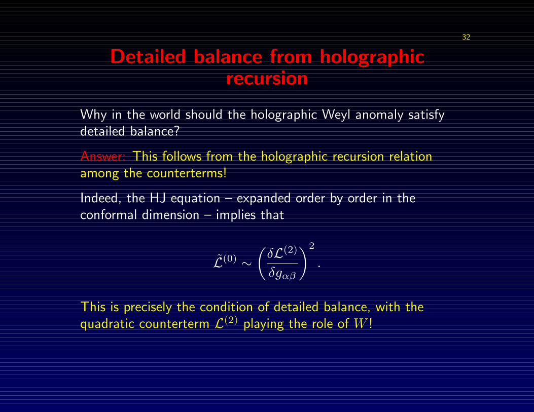
32

Detailed balance from holographicrecursion

Why in the world should the holographic Weyl anomaly satisfydetailed balance?

Answer: This follows from the holographic recursion relationamong the counterterms!

Indeed, the HJ equation – expanded order by order in theconformal dimension – implies that

L(0) ∼(δL(2)

δgαβ

)2

.

This is precisely the condition of detailed balance, with thequadratic counterterm L(2) playing the role of W !

33

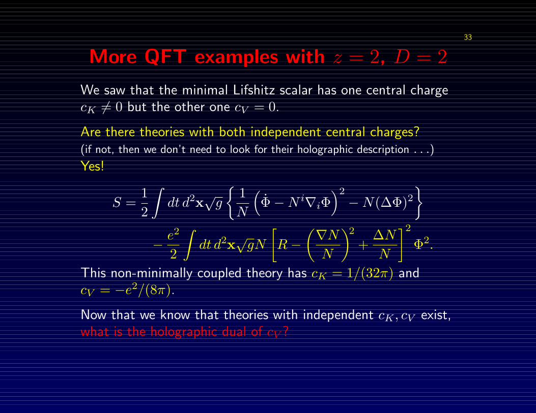
More QFT examples with z = 2, D = 2

We saw that the minimal Lifshitz scalar has one central chargecK 6= 0 but the other one cV = 0.

Are there theories with both independent central charges?(if not, then we don’t need to look for their holographic description . . .)

33

More QFT examples with z = 2, D = 2

We saw that the minimal Lifshitz scalar has one central chargecK 6= 0 but the other one cV = 0.

Are there theories with both independent central charges?(if not, then we don’t need to look for their holographic description . . .)

Yes!

S =12

∫dt d2x

√g

1N

(Φ−N i∇iΦ

)2

−N(∆Φ)2

− e

2

2

∫dt d2x

√gN

[R−

(∇NN

)2

+∆NN

]2

Φ2.

This non-minimally coupled theory has cK = 1/(32π) andcV = −e2/(8π).

Now that we know that theories with independent cK, cV exist,what is the holographic dual of cV ?

34

Holography with the general anomaly?

•The simplest relativistic system does not work.

• If looking for a more complicated relativistic model:Need to relax the holographic recursion between counterterms,

L(0) 6=(δL(2)

δgαβ

)2

.

• But: it turns out that Lifshitz gravity works, in the vacuum!

Disclaimer: That does not imply that one cannot do this with relativistic

gravity coupled to matter; indeed, the boundary between relativistic and

nonrelativistic is somewhat fuzzy.)

35

IIb.Lifshitz holography with Lifshitz gravity

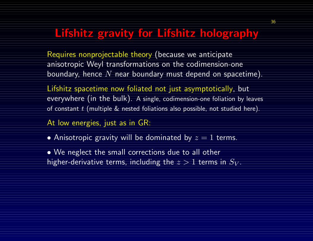
36

Lifshitz gravity for Lifshitz holography

Requires nonprojectable theory (because we anticipateanisotropic Weyl transformations on the codimension-oneboundary, hence N near boundary must depend on spacetime).

Lifshitz spacetime now foliated not just asymptotically, buteverywhere (in the bulk). A single, codimension-one foliation by leaves

of constant t (multiple & nested foliations also possible, not studied here).

At low energies, just as in GR:

• Anisotropic gravity will be dominated by z = 1 terms.

• We neglect the small corrections due to all otherhigher-derivative terms, including the z > 1 terms in SV .

37

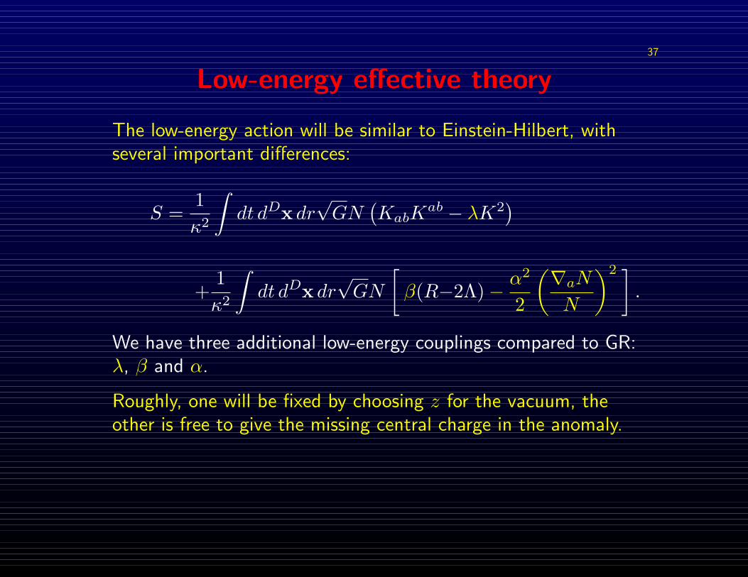
Low-energy effective theory

The low-energy action will be similar to Einstein-Hilbert, withseveral important differences:

S =1κ2

∫dt dDx dr

√GN

(KabK

ab − λK2)

+1κ2

∫dt dDx dr

√GN

[β(R−2Λ)− α

2

2

(∇aNN

)2 ].

We have three additional low-energy couplings compared to GR:λ, β and α.

Roughly, one will be fixed by choosing z for the vacuum, theother is free to give the missing central charge in the anomaly.

38

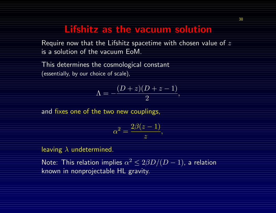
Lifshitz as the vacuum solutionRequire now that the Lifshitz spacetime with chosen value of zis a solution of the vacuum EoM.

This determines the cosmological constant(essentially, by our choice of scale),

Λ = −(D + z)(D + z − 1)2

,

and fixes one of the two new couplings,

α2 =2β(z − 1)

z,

leaving λ undetermined.

Note: This relation implies α2 ≤ 2βD/(D − 1), a relationknown in nonprojectable HL gravity.

39

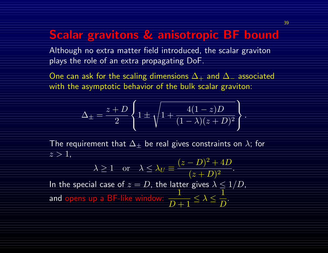
Scalar gravitons & anisotropic BF boundAlthough no extra matter field introduced, the scalar gravitonplays the role of an extra propagating DoF.

One can ask for the scaling dimensions ∆+ and ∆− associatedwith the asymptotic behavior of the bulk scalar graviton:

∆± =z +D

2

1±

√1 +

4(1− z)D(1− λ)(z +D)2

.

The requirement that ∆± be real gives constraints on λ; forz > 1,

λ ≥ 1 or λ ≤ λU ≡(z −D)2 + 4D

(z +D)2.

In the special case of z = D, the latter gives λ ≤ 1/D,

and opens up a BF-like window:1

D + 1≤ λ ≤ 1

D.

40

Holographic recursion in HL gravity:The counterterms and the anomaly

Again, use the radial Hamilton-Jacobi formulation to performholographic renormalization. Logic is identical to the relativisticcase.

In the special case of D = 2, z = 2, we found the general formof the anisotropic Weyl anomaly:

12κ2

(KijK

ij − 12K2

)+

β

48κ2

[R−

(∇NN

)2

+∆NN

]2

.

Thus, both cK and cV are independently produced inholographic renormalization of minimal HL gravity in thevacuum.

41

III.Black holes & Conclusions

42

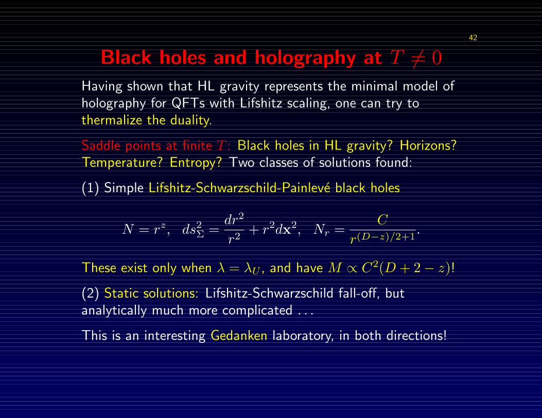
Black holes and holography at T 6= 0Having shown that HL gravity represents the minimal model ofholography for QFTs with Lifshitz scaling, one can try tothermalize the duality.

Saddle points at finite T : Black holes in HL gravity? Horizons?Temperature? Entropy? Two classes of solutions found:

(1) Simple Lifshitz-Schwarzschild-Painleve black holes

N = rz, ds2Σ =

dr2

r2+ r2dx2, Nr =

C

r(D−z)/2+1.

These exist only when λ = λU , and have M ∝ C2(D + 2− z)!

(2) Static solutions: Lifshitz-Schwarzschild fall-off, butanalytically much more complicated . . .

This is an interesting Gedanken laboratory, in both directions!

43

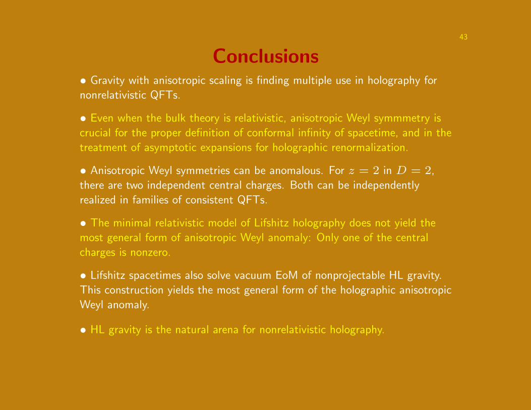
Conclusions• Gravity with anisotropic scaling is finding multiple use in holography for

nonrelativistic QFTs.

• Even when the bulk theory is relativistic, anisotropic Weyl symmmetry is

crucial for the proper definition of conformal infinity of spacetime, and in the

treatment of asymptotic expansions for holographic renormalization.

• Anisotropic Weyl symmetries can be anomalous. For z = 2 in D = 2,

there are two independent central charges. Both can be independently

realized in families of consistent QFTs.

• The minimal relativistic model of Lifshitz holography does not yield the

most general form of anisotropic Weyl anomaly: Only one of the central

charges is nonzero.

• Lifshitz spacetimes also solve vacuum EoM of nonprojectable HL gravity.

This construction yields the most general form of the holographic anisotropic

Weyl anomaly.

• HL gravity is the natural arena for nonrelativistic holography.