bernese gps software version 5.0 tutorial
TRANSCRIPT

Bernese GPS Software
Version 5.0
Tutorial
Processing ExampleIntroductory Course
Terminal Session
Rolf Dach, Urs Hugentobler,
Pierre Fridez
February 2007
AIUB Astronomical Institute, University of Bern


Contents
1. Introduction to the Example Campaign 1
2. Terminal Session: Monday 3
2.1 Start the Menu . . . . . . . . . . . . . . . . . . . . . . . . . . . . . . . . . . 3
2.2 Select Current Session . . . . . . . . . . . . . . . . . . . . . . . . . . . . . . 3
2.3 Campaign Setup . . . . . . . . . . . . . . . . . . . . . . . . . . . . . . . . . 4
2.4 Input Files for the Processing Examples . . . . . . . . . . . . . . . . . . . . 7
2.4.1 Atmosphere files ATM . . . . . . . . . . . . . . . . . . . . . . . . . . 7
2.4.2 General files GEN . . . . . . . . . . . . . . . . . . . . . . . . . . . . 7
2.4.3 Orbit files ORB . . . . . . . . . . . . . . . . . . . . . . . . . . . . . 7
2.4.4 RINEX files ORX, OUT . . . . . . . . . . . . . . . . . . . . . . . . . 8
2.4.5 Station files STA . . . . . . . . . . . . . . . . . . . . . . . . . . . . 8
2.5 Menu Variables . . . . . . . . . . . . . . . . . . . . . . . . . . . . . . . . . . 9
2.6 Generate A priori Coordinates . . . . . . . . . . . . . . . . . . . . . . . . . 11
2.7 Importing the Observations . . . . . . . . . . . . . . . . . . . . . . . . . . . 13
2.8 Daily Goals . . . . . . . . . . . . . . . . . . . . . . . . . . . . . . . . . . . . 17
3. Terminal Session: Tuesday 18
3.1 Prepare Pole Information . . . . . . . . . . . . . . . . . . . . . . . . . . . . 18
3.2 Generate Orbit Files . . . . . . . . . . . . . . . . . . . . . . . . . . . . . . . 20
3.3 Data Preprocessing (I) . . . . . . . . . . . . . . . . . . . . . . . . . . . . . . 26
3.3.1 Receiver Clock Synchronization . . . . . . . . . . . . . . . . . . . . 26
3.3.2 Form Baselines . . . . . . . . . . . . . . . . . . . . . . . . . . . . . 29
3.3.3 Preprocessing of the Phase Baseline Files . . . . . . . . . . . . . . 31
3.4 Daily Goals . . . . . . . . . . . . . . . . . . . . . . . . . . . . . . . . . . . . 35
Bernese GPS Software Version 5.0 Page I

Contents
4. Terminal Session: Wednesday 36
4.1 Data Preprocessing (II) . . . . . . . . . . . . . . . . . . . . . . . . . . . . . 36
4.2 Make a First Network Solution . . . . . . . . . . . . . . . . . . . . . . . . . 43
4.3 Ambiguity Resolution (QIF) . . . . . . . . . . . . . . . . . . . . . . . . . . 46
4.4 Daily Goals . . . . . . . . . . . . . . . . . . . . . . . . . . . . . . . . . . . . 58
5. Terminal Session: Thursday 59
5.1 Final Network Solution . . . . . . . . . . . . . . . . . . . . . . . . . . . . . 59
5.2 Check the Coordinates of the Fiducial Sites . . . . . . . . . . . . . . . . . . 65
5.3 Check the Daily Repeatability . . . . . . . . . . . . . . . . . . . . . . . . . 71
5.4 Compute the Final Solution of the Session . . . . . . . . . . . . . . . . . . 73
5.5 Velocity Estimation . . . . . . . . . . . . . . . . . . . . . . . . . . . . . . . 76
5.6 Daily Goals . . . . . . . . . . . . . . . . . . . . . . . . . . . . . . . . . . . . 83
6. Terminal Session: Friday 84
6.1 Kinematic Positioning . . . . . . . . . . . . . . . . . . . . . . . . . . . . . . 84
6.2 Clock Estimation . . . . . . . . . . . . . . . . . . . . . . . . . . . . . . . . . 88
6.3 Bernese Processing Engine . . . . . . . . . . . . . . . . . . . . . . . . . . . 96
Page II AIUB

1. Introduction to the Example Campaign
Data from eight European stations of theIGS Network are selected for the examplecampaign. They are listed in Table 1.1 to-gether with the receiver and antenna typeand the antenna height. The locations ofthese stations are given in Figure 1.1.
Three of these stations (MATE, ONSA, andVILL) are IGS core sites. This is a set ofabout 95 IGS stations representing the real-ization of the reference frame (IGS 00: IGSrealization of the ITRF 2000).
Furthermore, two stations (FFMJ andZIMJ) are equipped with GNSS receiverstracking GPS and GLONASS satellites. Thereceiver antennas of only two sites (ONSAand PTBB) are equipped with radomes (type OSOD resp. SNOW).
BRUS -- FFMJ
- MATE
- ONSA
- PTBB
- VILL
ZIMM -- ZIMJ
Figure 1.1: Stations used in example campaign
The receivers used at the stations BRUS and PTBB are connected to H-Maser. The receivertype ASHTECH Z-XII3T was developed for time and frequency applications.
The distances between neighboring stations are between 300 and 1200 km. Two GPS re-ceivers in Zimmerwald are included into the example (ZIMM and ZIMJ, distance 14 m).
The observations for these stations are available for four days. Two days in year 2002 (dayof year 143 and 144) and two in 2003 (days 138 and 139). In these terminal sessions youwill analyze the data in order to obtain a velocity field based on IGS final products.
The data belonging to this example campaign are included in the distribution. Therefore,you may also use this document to repeat the generation of the solution at home to exercisethe use of the Bernese GPS Software.
Bernese GPS Software Version 5.0 Page 1

1. Introduction to the Example Campaign
Table 1.1: List of stations used for the example campaign including receiver and antennatype as well as the antenna height.
Station name Location Receiver type AntennaAntenna type Radome height
BRUS 13101M004 Brussels, Belgium ASHTECH Z-XII3TASH701945B M NONE 3.9702 m
FFMJ 14279M001 Frankfurt (Main), Germany JPS LEGACYJPSREGANT SD E NONE 0.0000 m
MATE 12734M008 Matera, Italy TRIMBLE 4000SSITRM29659.00 NONE 0.1010 m
ONSA 10402M004 Onsala, Sweden ASHTECH Z-XII3AOAD/M B OSOD 0.9950 m
PTBB 14234M001 Braunschweig, Germany ASHTECH Z-XII3TASH700936E SNOW 0.0562 m
VILL 13406M001 Villafranca, Spain ASHTECH Z-XII3AOAD/M T NONE 0.0437 m
ZIMJ 14001M006 Zimmerwald, Switzerland JPS LEGACYJPSREGANT SD E NONE 0.0770 m
ZIMM 14001M004 Zimmerwald, Switzerland TRIMBLE 4000SSITRM29659.00 NONE 0.0000 m
Page 2 AIUB

2. Terminal Session: Monday
Today’s terminal session is to
(1) become familiar with the UNIX environment, the menu of the Bernese GPSSoftware, and the example campaign,
(2) verify the campaign setup done for you (see sections 2.2 and 2.3, and alsothe handout for the terminal sessions),
(3) generate the a priori coordinates for all 4 days using COOVEL (see Section2.6 ), and
(4) import the observations from the RINEX into the Bernese format for all fourdays of the example using RNXOBV3 (section 2.7).
2.1 Start the Menu
Start the menu program using the command G1.
Navigate through the submenus to become familiar with the structure of the menu. Readthe general help (available at ”Menu>Help>General”) to get an overview on the usage of themenu program of the Bernese GPS Software.
For the terminal session in the Bernese introduction course, the campaign setup has alreadybeen done for each user. Please check that the campaign name in the statusbar of the BerneseMenu is set correctly to your campaign (refer to the separate handout) and that the currentsession is set to the first session (i.e. $Y+0=2002, $S+0=1430). If this is not the case, pleaseask for help.
2.2 Select Current Session
Select ”Menu>Campaign>Edit session table” to check the session table. It is recommended to use thewildcard string ???0 for the “SESSion identifier” in panel “SESSION TABLE”. The panel belowshows the session definition for a typical permanent campaign with 24-hours sessions. Thesetup of the session table is a very important task when you prepare a campaign. Pleaseread the corresponding online help carefully.
1At the exercise terminals the Bernese environment is loaded automatically during the login. At homeyou have to source the file ${X}/EXE/LOADGPS.setvar on UNIX–platforms either manually or during thelogin.
Bernese GPS Software Version 5.0 Page 3

2. Terminal Session: Monday
Save the session table (press the ^Save button) and open the “Date Selection Dialogue” the”Menu>Configure>Set session/compute date” in order to define the current session:
2.3 Campaign Setup
Usually, a new campaign must first be added to the campaign list (”Menu>Campaign>Edit list
of campaigns”) and set as active campaign (”Menu>Campaign>Select active campaign”), before the di-rectory structure can be created (”Menu>Campaign>Create new campaign”. This is already done foryour campaign, but you should verify that this is correctly done. In order to become fa-miliar with the campaign structure, you can now visit your campaign directory and inspectthe contents using the command line (using cd and ls for changing directories and creatingdirectory listings, respectively.
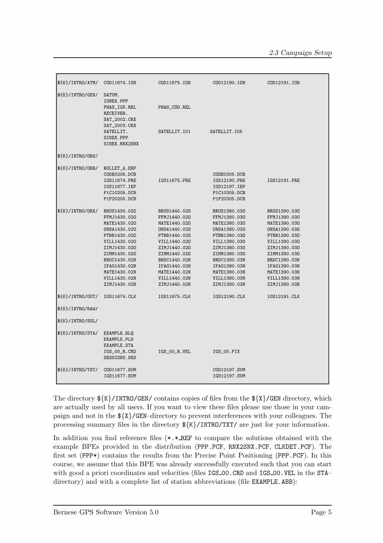
You will find the following directories and input data for the processing of the example cam-paign (note that ${K}/INTRO is used in this document in place of your individual campaignname):
Page 4 AIUB
2.3 Campaign Setup
${K}/INTRO/ATM/ COD11674.ION COD11675.ION COD12190.ION COD12191.ION
${K}/INTRO/GEN/ DATUM.
IONEX.PPP
PHAS_IGS.REL PHAS_COD.REL
RECEIVER.
SAT_2002.CRX
SAT_2003.CRX
SATELLIT. SATELLIT.I01 SATELLIT.I05
SINEX.PPP
SINEX.RNX2SNX
${K}/INTRO/OBS/
${K}/INTRO/ORB/ BULLET_A.ERP
CODE0205.DCB CODE0305.DCB
IGS11674.PRE IGS11675.PRE IGS12190.PRE IGS12191.PRE
IGS11677.IEP IGS12197.IEP
P1C10205.DCB P1C10305.DCB
P1P20205.DCB P1P20305.DCB
${K}/INTRO/ORX/ BRUS1430.02O BRUS1440.02O BRUS1380.03O BRUS1390.03O
FFMJ1430.02O FFMJ1440.02O FFMJ1380.03O FFMJ1390.03O
MATE1430.02O MATE1440.02O MATE1380.03O MATE1390.03O
ONSA1430.02O ONSA1440.02O ONSA1380.03O ONSA1390.03O
PTBB1430.02O PTBB1440.02O PTBB1380.03O PTBB1390.03O
VILL1430.02O VILL1440.02O VILL1380.03O VILL1390.03O
ZIMJ1430.02O ZIMJ1440.02O ZIMJ1380.03O ZIMJ1390.03O
ZIMM1430.02O ZIMM1440.02O ZIMM1380.03O ZIMM1390.03O
BRDC1430.02N BRDC1440.02N BRDC1380.03N BRDC1390.03N
IFAG1430.02N IFAG1440.02N IFAG1380.03N IFAG1390.03N
MATE1430.02N MATE1440.02N MATE1380.03N MATE1390.03N
VILL1430.02N VILL1440.02N VILL1380.03N VILL1390.03N
ZIMJ1430.02N ZIMJ1440.02N ZIMJ1380.03N ZIMJ1390.03N
${K}/INTRO/OUT/ IGS11674.CLK IGS11675.CLK IGS12190.CLK IGS12191.CLK
${K}/INTRO/RAW/
${K}/INTRO/SOL/
${K}/INTRO/STA/ EXAMPLE.BLQ
EXAMPLE.PLD
EXAMPLE.STA
IGS_00_R.CRD IGS_00_R.VEL IGS_00.FIX
SESSIONS.SES
${K}/INTRO/TXT/ COD11677.SUM COD12197.SUM
IGS11677.SUM IGS12197.SUM
The directory ${K}/INTRO/GEN/ contains copies of files from the ${X}/GEN directory, whichare actually used by all users. If you want to view these files please use those in your cam-paign and not in the ${X}/GEN–directory to prevent interferences with your colleagues. Theprocessing summary files in the directory ${K}/INTRO/TXT/ are just for your information.
In addition you find reference files (*.* REF to compare the solutions obtained with theexample BPEs provided in the distribution (PPP.PCF, RNX2SNX.PCF, CLKDET.PCF). Thefirst set (PPP*) contains the results from the Precise Point Positioning (PPP.PCF). In thiscourse, we assume that this BPE was already successfully executed such that you can startwith good a priori coordinates and velocities (files IGS 00.CRD and IGS 00.VEL in the STA–directory) and with a complete list of station abbreviations (file EXAMPLE.ABB):
Bernese GPS Software Version 5.0 Page 5

2. Terminal Session: Monday
${K}/INTRO/ATM/ RIM021430.INX_REF RIM021440.INX_REF RIM031380.INX_REF RIM031390.INX_REF
${K}/INTRO/GEN/
${K}/INTRO/OBS/
${K}/INTRO/ORB/
${K}/INTRO/ORX/
${K}/INTRO/OUT/ PPP021430.PRC_REF PPP021440.PRC_REF PPP031380.PRC_REF PPP031390.PRC_REF
PPP021430.CLK_REF PPP021440.CLK_REF PPP031380.CLK_REF PPP031390.CLK_REF
PPP021430.OUT_REF PPP021440.OUT_REF PPP031380.OUT_REF PPP031390.OUT_REF
${K}/INTRO/RAW/
${K}/INTRO/SOL/
${K}/INTRO/STA/ EXAMPLE.ABB_REF
IGS_00.CRD_REF IGS_00.VEL_REF
PPP021430.CRD_REF PPP021440.CRD_REF PPP031380.CRD_REF PPP031390.CRD_REF
REF021430.CRD_REF REF021440.CRD_REF REF031380.CRD_REF REF031390.CRD_REF
${K}/INTRO/TXT/
In the terminal session we will more or less follow the example BPE RNX2SNX.PCF to computestation coordinates and troposphere parameters for a regional GNSS network. As we willpractice the topics of the theoretical morning lessons in these terminal sessions, we will notstrictly follow all steps of this example BPE. The reference solutions from this example are:
${K}/INTRO/ATM/ F1_021430.TRP_REF F1_021440.TRP_REF F1_031380.TRP_REF F1_031390.TRP_REF
${K}/INTRO/GEN/
${K}/INTRO/OBS/
${K}/INTRO/ORB/
${K}/INTRO/ORX/
${K}/INTRO/OUT/ R2S021430.PRC_REF R2S021440.PRC_REF R2S031380.PRC_REF R2S031390.PRC_REF
F1_021430.OUT_REF F1_021440.OUT_REF F1_031380.OUT_REF F1_031390.OUT_REF
${K}/INTRO/RAW/
${K}/INTRO/SOL/ F1_021430.SNX_REF F1_021440.SNX_REF F1_031380.SNX_REF F1_031390.SNX_REF
${K}/INTRO/STA/ F1_021430.CRD_REF F1_021440.CRD_REF F1_031380.CRD_REF F1_031390.CRD_REF
${K}/INTRO/TXT/
Another example provided in the distribution concerns the estimation of receiver and satel-lite clock corrections starting from the broadcast navigation messages (CLKDET.PCF). Youmay use the terminal session on Thursday or Friday to follow this example. The referenceresult files are:
Page 6 AIUB

2.4 Input Files for the Processing Examples
${K}/INTRO/ATM/
${K}/INTRO/GEN/
${K}/INTRO/OBS/
${K}/INTRO/ORB/ TT_021430.CLK_REF TT_021440.CLK_REF TT_031380.CLK_REF TT_031390.CLK_REF
${K}/INTRO/ORX/
${K}/INTRO/OUT/ CLK021430.PRC_REF CLK021440.PRC_REF CLK031380.PRC_REF CLK031390.PRC_REF
TT_021430.CLK_REF TT_021440.CLK_REF TT_031380.CLK_REF TT_031390.CLK_REF
TTG021430.OUT_REF TTG021440.OUT_REF TTG031380.OUT_REF TTG031390.OUT_REF
${K}/INTRO/RAW/
${K}/INTRO/SOL/
${K}/INTRO/STA/
${K}/INTRO/TXT/
2.4 Input Files for the Processing Examples
2.4.1 Atmosphere files ATM
The input files in this directory are global ionosphere models in the Bernese format obtainedfrom the IGS processing at CODE. They will be used to resolve the phase ambiguities usingthe QIF–strategy (QIF: Quasi–Ionosphere–Free).
2.4.2 General files GEN
These general input files contain information that is neither user- nor campaign-specific.They are accessed by all users, and changes in this files will affect processing for everyone.Consequently, these files are located in the ${X}/GEN directory. Table 2.1 shows the list ofgeneral files necessary for the processing example. It also shows which files need updatingfrom time to time by downloading them from the anonymous ftp–server of AIUB (http://www.aiub.unibe.ch/download/BSWUSER50/GEN).
Each Bernese processing program has its own panel for general files. Make sure that youuse the correct files listed in Table 2.1 .
Copies of these files are available in your campaign’s GEN–directory. In order to prevent ac-cidental change of the ”live” files in ${X}/GEN, we recommend that you only inspect/browsethe files in your campaign area.
2.4.3 Orbit files ORB
The precise orbits in the files *.PRE are the combined final products from the IGS. Theydo not contain orbits for the GLONASS satellites. The corresponding Earth orientationparameters are given in weekly files with the extension *.IEP .
Bernese GPS Software Version 5.0 Page 7

2. Terminal Session: Monday
Table 2.1: List of general files to be used in the Bernese programs for the processingexample.
Filename Content Modification DownloadCONST. All constants used in the No BSW aftp
Bernese GPS SoftwareDATUM. Definition of geodetic datum Introducing new reference BSW aftp
ellipsoidRECEIVER. Receiver information Introducing new receiver type BSW aftpPHAS COD.REL Phase center eccentricities Introducing new elevation- BSW aftp
and variations including dependent correctionsradome codes New antenna
SATELLIT.I01 Satellite information file New launched satellites BSW aftpSAT $Y+0.CRX Satellite problems Satellite maneuvers, bad data, ... BSW aftpGPSUTC. Leap seconds When a new leap second is BSW aftp
announced by the IERSIAU2000.NUT Nutation model coefficients No —IERS2000.SUB Subdaily pole model No —
coefficients —POLOFF. Pole offset coefficients Introducing new values from —
IERS annual report (until 1997)JGM3. Earth potential coefficients No —OT CSRC.TID Ocean tides coefficients No —SINEX. SINEX header information Adapt SINEX header for —SINEX.TRO your institutionSINEX.PPP . . . for the PPP exampleSINEX.RNX2SNX . . . for the double–diff. exampleIONEX. IONEX header information Adapt IONEX header for —
your institutionIONEX.PPP . . . for the PPP example
Furthermore, the directory contains monthly means for the differential code biases (DCBs).
2.4.4 RINEX files ORX, OUT
The raw data are given in RINEX format. The observations *.$YO ($Y is the menu time vari-able for the two–digit year of the current session) are used for all examples. The navigationmessages *.$YN are only used for the clock determination example.
The clock RINEX files are located in the OUT–directory. They are consistent with the IGSorbit and ERP products in the ORB–directory. They contain station and satellite clockcorrections with 5 min. sampling.
2.4.5 Station files STA
The a priori coordinates of the stations in the IGS realization of the reference frameITRF2000 are available in the file IGS 00.CRD . It was generated using the PPP exam-ple for day 143 of year 2002. It contains all IGS core sites (copied from file IGS 00 R.CRD —the IGS realization of the reference frame ITRF2000) and the PPP results for the remaining
Page 8 AIUB

2.5 Menu Variables
stations. The epoch of the coordinates is January 01, 2000. The corresponding velocity fileIGS 00.VEL contains the velocities for the core sites (copied from file IGS 00 R.VEL) com-pleted by the NNR-NUVEL1A velocities for the other stations. The assignment of stationsto tectonic plates is given in the file EXAMPLE.PLD. The file IGS 00.FIX contains the list ofall IGS core sites. It will be useful to define the geodetic datum when estimating station co-ordinates. You can browse all these files with a text editor or with the menu (”Menu>Campaign
>Edit station files”).
To make sure that you process the data in the Bernese GPS Software with correct sta-tion information (station name, receiver type, antenna type, antenna height, etc.) the fileEXAMPLE.STA is used to verify the RINEX header information. The reason to use this file hasto be seen in the fact that some antenna heights or receiver/antenna types in the RINEXfiles may not be correct or may be measured to a different antenna reference point. Similarly,the marker (station) names in the RINEX files may differ from the names we want to use inthe processing. The antenna types have to correspond to those in the file PHAS COD.REL inorder that the correct phase center offsets and variations are used. The receiver types haveto be defined in the RECEIVER. file to correctly apply the DCB corrections.
The last file to be mentioned in this list is EXAMPLE.BLQ. It provides the coefficients for theocean tidal loading of the stations to be processed. It has to be applied at least in the finalrun of GPSEST.
2.5 Menu Variables
When processing GNSS data, it is often necessary to repeat a program run several times withonly slightly different option settings. A typical example would be the processing of severalsessions of data. The names of observation files change from session to session because thesession number is typically a part of the file name. It would be very cumbersome to repeatall the runs selecting the correct files manually every time. For the BPE an automatizationis mandatory. For such cases the Bernese menu system provides a powerful tool — so–called menu variables. The menu variables are defined in the user–specific menu input file${U}/PAN/MENU VAR.INP that is accessible through ”Menu>Configure>Menu variables”. Three kindsof menu–variables are available: predefined variables (also called menu time variables), user–defined variables, and system environment variables.
The use of system environment variables is necessary to generate the complete pathto the files used in the Bernese GPS Software. The campaign data are located in thedirectory ${K}/INTRO=/aiub u camp/INTRO. The user–dependent files can be found at${U}=/u/aiub/bern50/GPSUSER — note, that you will find instead of bern50 your username in the path. The temporary user files are saved in ${T}=/scratch/bern50. Finally,the campaign–independent files reside in ${X}=/aiub sw/BERN50/GPS.
Bernese GPS Software Version 5.0 Page 9

2. Terminal Session: Monday
The predefined variables provide a set of time strings assigned to the current session. Fromthe second panel of the menu variables you may get an overview on the available variablesand their usage:
Be aware that the variable $S+1 refers to the next session. Because we are using a sessiontable for a daily processing it also corresponds to the next day.
Page 10 AIUB

2.6 Generate A priori Coordinates
These variables are automaticall translated by the menu upon saving the panel or runningthe program. We recommend to make use of them in the input panels (e.g. for filenamespecification).
2.6 Generate A priori Coordinates
As stated before the a priori coordinates generated from the PPP example BPE refer to theepoch January 01, 2000 . The first step is to extrapolate the coordinates to the epoch thatis currently processed. The program COOVEL is used for this purpose. Open the programinput panel in ”Menu>Service>Coordinate tools>Extrapolate coordinates”:
“REFERENCE EPOCH” $YMD STR+0 → 2002 05 23
“Output coordinate file” APR$YD+0 → APR02143
“TITLE” Session $YSS+0: → Session 021430:
Start the program with the ^Run–button. The program generates an output file COOVEL.L*
in the directory ${K}/INTRO/OUT. This file may be browsed using the ^Output–button orwith ”Menu>Service>Browse program output” . It should look like
Bernese GPS Software Version 5.0 Page 11

2. Terminal Session: Monday
===============================================================================
Program : coovel Bernese GPS Software Version 5.0
Purpose : Propagation of coordinates with a given velocity field
Campaign: ${K}/INTRO Default session: 1430 year 2002
Date : 13-Feb-2007 11:22 User name : bern50
===============================================================================
EXAMPLE: Session 021430: Coordinate propagation
-------------------------------------------------------------------------------
INPUT AND OUTPUT FILENAMES
--------------------------
-------------------------------------------------------------------------------
Session table : ${K}/INTRO/STA/SESSIONS.SES
Input coordinate file : ${K}/INTRO/STA/IGS_00.CRD
Output coordinate file : ${K}/INTRO/STA/APR02143.CRD
Input velocity file : ${K}/INTRO/STA/IGS_00.VEL
Program output : ${K}/INTRO/OUT/COOVEL.L00
Error message : ${U}/WORK/ERROR.MSG
-------------------------------------------------------------------------------
...
The header area of the program output is standardized for all programs of the Bernese GPSSoftware, Version 5.0 . Furthermore each program has a title line that should characterizethe program run. It is printed to the program output and to most of the result files. Manyprogram output files furthermore provide a list of input and output files that have beenused or generated.
The result of the run of COOVEL is an a priori coordinate file(${K}/INTRO/STA/APR02143.CRD) containing the positions of the sites to be pro-cessed for the epoch of the current session (the lines for the other stations are ignored inthe processing):
IGS00 COORDINATES BASED ON IGS01P37_RS54.SNX 29-JUN-03
--------------------------------------------------------------------------------
LOCAL GEODETIC DATUM: IGS00 EPOCH: 2002-05-23 0:00:00
NUM STATION NAME X (M) Y (M) Z (M) FLAG
6 BRUS 13101M004 4027893.7773 307045.7760 4919475.0809 PPP
15 FFMJ 14279M001 4053455.9006 617729.6193 4869395.6681 PPP
36 MATE 12734M008 4641949.6104 1393045.3794 4133287.4177 IGS00
42 ONSA 10402M004 3370658.5806 711877.1009 5349786.9189 IGS00
47 PTBB 14234M001 3844059.9795 709661.2696 5023129.5003 PPP
56 VILL 13406M001 4849833.7343 -335049.0774 4116014.9013 IGS00
63 ZIMJ 14001M006 4331293.9550 567542.0890 4633135.6788 PPP
64 ZIMM 14001M004 4331297.0935 567555.8333 4633133.8919 PPP
Repeat this step for the other three sessions of the example by changing the current sessionusing ”Menu>Configure>Set session/compute date”. You can then use the Rer^un button to restartthe program. No options need to be changed since consequent use of the menu time variableswas made.
Page 12 AIUB

2.7 Importing the Observations
2.7 Importing the Observations
The campaign has now been set up and all necessary files are available. The first part ofprocessing consists of the transfer of the observations from RINEX to Bernese (binary)format. To get an overview of the data availability you may generate a pseudographic fromthe RINEX observation files using the program RNXGRA in ”Menu>RINEX>RINEX utilities>Create
observation statistics” — this step is not mandatory but it may be useful to get an impression ofthe tracking performance of the stations before you start the analysis.
Importing the RINEX observation files is the task of the program RXOBV3 in ”Menu>RINEX
>Import RINEX to Bernese format>Observation files” (we do not use the RINEX navigation files for thisprocessing example). You need to run this program for all 4 sessions of the example.
All RINEX observation files fitting ${K}/INTRO/RAW/????1430.02O are selected automati-cally by the current entry in the input field “original RINEX observation files”. You can verifythis by pressing the button just right from this input field (labeled with the file extension02O). In the file selection dialogue you will see the list of currently selected files. The RINEXfiles of the year 2003 are shown if a current session from the year 2003 is selected. In thatcase the label of the button changes to 03O.
Bernese GPS Software Version 5.0 Page 13

2. Terminal Session: Monday
The next panel specifies the general input files. There are three further panels defining theinput options for RXOBV3. They allow to select the data to be imported and to specify afew parameters for the Bernese observation header files:
We select GPS for the option “Satellite system to be considered” because the IGS orbits provideonly the positions of the GPS satellites.
Page 14 AIUB

2.7 Importing the Observations
Two more panels provide options to verify the RINEX header information:
Start the program with the ^Run–button.
Bernese GPS Software Version 5.0 Page 15

2. Terminal Session: Monday
A warning message will appear to inform you that the observations to the GLONASS satel-lites (satellite system R) are removed from the two stations equipped with GNSS receivers.
### PG RXOBV3: OBSERVATION DATA FROM OTHER SATELLITE SYSTEM REJECTED
RINEX FILE NAME: ${K}/INTRO/RAW/FFMJ1430.02O
SR R2RDOR: SATELLITES SKIPPED! SYSTEM: "R"
### PG RXOBV3: OBSERVATION DATA FROM OTHER SATELLITE SYSTEM REJECTED
RINEX FILE NAME: ${K}/INTRO/RAW/ZIMJ1430.02O
The program produces an output file RXO02143.OUT in the directory ${K}/INTRO/OUT (resp.corresponding filenames for the other sessions). This file may be browsed using the ^Outputbutton or with ”Menu>Service>Browse program output” . After echoing the input options the fileprovides an overview of the station information records in the RINEX observation fileheader and the values that are used for the processing in the Bernese GPS Software. Inaddition some observation statistics are available. In the following section you may checkthe completeness of the Bernese observation files by the available number of epochs:
...
TABLE OF INPUT AND OUTPUT FILE NAMES:
------------------------------------
Num Rinex file name Bernese code header file name #epo ...
Bernese code observ. file name
Bernese phase header file name #epo ...
Bernese phase observ. file name
------------------------------------------------------------------------------- ...
1 ${K}/INTRO/RAW/BRUS1430.02O ${K}/INTRO/OBS/BRUS1430.CZH 2778 ...
${K}/INTRO/OBS/BRUS1430.CZO
${K}/INTRO/OBS/BRUS1430.PZH 2778 ...
${K}/INTRO/OBS/BRUS1430.PZO
2 ${K}/INTRO/RAW/FFMJ1430.02O ${K}/INTRO/OBS/FFMJ1430.CZH 2799 ...
${K}/INTRO/OBS/FFMJ1430.CZO
${K}/INTRO/OBS/FFMJ1430.PZH 2799 ...
${K}/INTRO/OBS/FFMJ1430.PZO
3 ${K}/INTRO/RAW/MATE1430.02O ${K}/INTRO/OBS/MATE1430.CZH 2880 ...
${K}/INTRO/OBS/MATE1430.CZO
${K}/INTRO/OBS/MATE1430.PZH 2880 ...
${K}/INTRO/OBS/MATE1430.PZO
...
If epochs are missing for some RINEX files you may check this with the RINEX observationgraphic from the program RNXGRA.
Page 16 AIUB

2.8 Daily Goals
2.8 Daily Goals
At the end of today’s session, you should have created the following files:
(1) a priori coordinates in your campaign’s STA directory: file APR02143.CRD,APR02144.CRD, ... (for all 4 days)
(2) Bernese formatted zero difference observation files in your campaign’s OBSdirectory:BRUS1430.CZH, BRUS1430.PZH, BRUS1430.CZO, BRUS1430.PZO, ...(for all stations).
These files must be generated for all four days.
Bernese GPS Software Version 5.0 Page 17

3. Terminal Session: Tuesday
Today’s terminal session is to
(1) generate the pole information file in Bernese format (POLUPD)
(2) generate tabular orbit files from IGS precise files (PRETAB)
(3) generate Bernese standard orbit files (ORBGEN)
(4) preprocess the Bernese observation files:
• receiver clock synchronization (CODSPP)
• baseline generation (SNGDIF)
• preprocess baselines (MAUPRP)
for all four days of the processing example. You can run all programs for one day,and then rerun them for the next day.
3.1 Prepare Pole Information
Together with the precise orbit files (PRE), a consistent set of Earth orientation informationis provided in the ORB–directory. Whereas the orbits are given in daily files the EOPs areavailable in weekly files for the IGS final product series. We have to convert the informationfrom the IERS/IGS standard format (file extension within the Bernese GPS Software isIEP) into the internal Bernese EOP format (file extension within the Bernese GPS Softwareis ERP). This is the task of the program POLUPD (”Menu>Orbits/EOP>Handle EOP files>Convert IERS
to Bernese format”) which is also able to update the EOP records to an existing file.
AIUB

3.1 Prepare Pole Information
Bernese GPS Software Version 5.0 Page 19

3. Terminal Session: Tuesday
The last panel for the program POLUPD is an example for the specification of time windowsin the Bernese GPS Software, Version 5.0 . Time windows can be defined by sessions (a singlesession or a range of sessions). Alternatively, a time window may be specified by a startand an end epoch. By entering either a start or an end epoch the user may define only thebeginning or the end of the time interval. We refer to the online help for more details.
The messages
### PG POLUPD: NUTATION MODEL NOT SPECIFIED IN INPUT ERP FILE
USING NUTATION MODEL NAME : IAU2000
### PG POLUPD: SUBDAILY POLE MODEL NOT SPECIFIED IN INPUT ERP FILE
USING SUBDAILY POLE MODEL NAME : IERS2000
just inform you that the subdaily pole and nutation model from the input panel is writtento the output file because no Bernese formatted ERP file was used as input.
3.2 Generate Orbit Files
In this processing example we use only two programs of the orbit part of the Bernese GPSSoftware. The first program is called PRETAB and may be accessed using ”Menu>Orbits/EOP
>Create tabular orbits”. The main task of PRETAB is to create tabular orbit files (TAB) (i.e., totransform the precise orbits from the terrestrial into the celestial reference frame) and togenerate a satellite clock file (CLK). The clock file will be needed in program CODSPP (seeSection 3.3.1) if no broadcast orbits are used.
Page 20 AIUB

3.2 Generate Orbit Files
Panel “PRETAB 3: Options for Clocks” contains the options for extracting the satellite clockinformation. The clock values in the precise orbit file are sampled to 15 min. We interpolatewith a “Polynomial degree” of 2 with an “Interval for polynomials” of 12 hours. This is goodenough for the receiver clock synchronization in CODSPP.
The second program of the orbit part used here is called ORBGEN (”Menu>Orbits/EOP>Create
standard orbits”). It prepares the so–called standard orbits using the satellite positions in thetabular orbit files as pseudo–observations for a least–squares adjustment.
Bernese GPS Software Version 5.0 Page 21

3. Terminal Session: Tuesday
Make sure that the EOP file, the nutation, and the subdaily pole model are the same youhave used in PRETAB. It is mandatory to use this triplet of files together with the generatedstandard orbits for all processing programs.
Page 22 AIUB

3.2 Generate Orbit Files
The “ORBIT MODEL IDENTIFIER” is used to check the consistency between input files andoptions. To generate standard orbits from IGS or CODE products use orbit model B. Ifthe JPL planetary ephemeris (DE200.EPH)is unavailable you may leave the correspondinginput field “Planetary ephemeris file” in the panel “ORBGEN 1.1: General Files” empty and setthe “ORBIT MODEL IDENTIFIER” to ? .
Bernese GPS Software Version 5.0 Page 23

3. Terminal Session: Tuesday
Page 24 AIUB

3.2 Generate Orbit Files
The program produces an output file ORB02143.OUT (or corresponding to the other sessions)which should look like
...
INPUT AND OUTPUT FILENAMES
--------------------------
-------------------------------------------------------------------------------
Session table : ${K}/INTRO/STA/SESSIONS.SES
General constants : ${X}/GEN/CONST.
Pole file : ${K}/INTRO/ORB/IGS02143.ERP
Subdaily pole model : ${X}/GEN/IERS2000.SUB
Nutation model : ${X}/GEN/IAU2000.NUT
Coeff. of Earth potential : ${X}/GEN/JGM3.
Satellite problems : ${X}/GEN/SAT_2002.CRX
Satellite information : ${X}/GEN/SATELLIT.I01
Planetary ephemeris file : ${X}/GEN/DE200.EPH
Ocean tides file : ${X}/GEN/OT_CSRC.TID
Orbital elements, file 1 : ---
Orbital elements, file 2 : ---
Standard orbits : ${K}/INTRO/ORB/IGS02143.STD
Radiation pressure coeff. : ---
Residual file : ---
Summary file : ${K}/INTRO/OUT/ORB02143.LST
Scratch file : ${U}/WORK/ORBGEN.SCR
Scratch file : ${U}/WORK/ORBGEN.SC2
Program output : ${K}/INTRO/OUT/ORB02143.OUT
Error message : ${U}/WORK/ERROR.MSG
-------------------------------------------------------------------------------
...
...
-------------------------------------------------------------------------------
RMS ERRORS AND MAX. RESIDUALS ARC NUMBER: 1 ITERATION: 2
-------------------------------------------------------------------------------
QUADRATIC MEAN OF O-C (M) MAX. RESIDUALS (M)
SAT #POS RMS (M) TOTAL RADIAL ALONG OUT RADIAL ALONG OUT
--- ---- ------- ----------------------------- --------------------
1 96 0.01 0.01 0.01 0.01 0.01 0.02 0.02 0.03
2 96 0.01 0.01 0.01 0.01 0.01 0.04 0.02 0.01
3 96 0.01 0.01 0.02 0.01 0.01 0.03 0.03 0.02
4 96 0.01 0.01 0.01 0.01 0.01 0.02 0.02 0.02
...
The most important information in the output file are the RMS errors for each satellite.These should not be larger than about 1. . . 2 cm if precise orbits were used together withthe consistent EOP information (the actual RMS errors depend on the quality of the preciseorbits, on the pole file used for the transformation between ITRF and ICRF in PRETAB,and on the orbit model used in ORBGEN).1
Comparing the RMS error from the second and the third iteration you will see that twoiterations should be already enough to produce precise standard orbits for GNSS satellites.
The file ${K}/INTRO/OUT/ORB02143.LST summarizing the orbit fit rms valuesmay be compared with the corresponding section in the solution reference file${K}/INTRO/OUT/R2S021430.PRC REF.
1You may check this statement by using the BULLET A.ERP file instead of the IGS02143.ERP. This is only
for a test — please, do not use the resulting standard orbit for any further processing!
Bernese GPS Software Version 5.0 Page 25

3. Terminal Session: Tuesday
3.3 Data Preprocessing (I)
3.3.1 Receiver Clock Synchronization
Now we are ready to invoke the processing part of the Bernese GPS Software. We have torun three programs for this example. The first program is called CODSPP (”Menu>Processing
>Code-based clock synchronization”. Its main task is to compute the receiver clock corrections.
Page 26 AIUB

3.3 Data Preprocessing (I)
We have already geocentric coordinates of good quality available for the sites from thePPP example BPE. Therefore, the option “Estimate coordinates” may be set to NO. The mostimportant option for this CODSPP run is “Save clock estimates”. It has to be set to BOTH.
Bernese GPS Software Version 5.0 Page 27

3. Terminal Session: Tuesday
CODSPP produces the following output:
...
STATION: BRUS 13101M004 FILE: ${K}/INTRO/OBS/BRUS1430.CZO RECEIVER UNIT: 0
-------------------------------------------------------------------------------------------
...
...
RESULTS:
--------
OBSERVATIONS IN FILE: 21844
BAD OBSERVATIONS : 0.15 %
RMS OF UNIT WEIGHT : 0.97 M
NUMBER OF ITERATIONS: 2
...
...
STATION COORDINATES:
--------------------
LOCAL GEODETIC DATUM: IGS00
A PRIORI NEW NEW- A PRIORI RMS ERROR
BRUS 13101M004 X 4027893.78 4027893.78 0.00 0.00
(MARKER) Y 307045.78 307045.78 0.00 0.00
Z 4919475.08 4919475.08 0.00 0.00
HEIGHT 149.66 149.66 0.00 0.00
LATITUDE 50 47 52.143 50 47 52.143 0 0 0.000 0.0000
LONGITUDE 4 21 33.186 4 21 33.186 0 0 0.000 0.0000
CLOCK PARAMETERS:
-----------------
OFFSET FOR REFERENCE EPOCH: 0.000000632 SEC
CLOCK OFFSETS STORED IN CODE+PHASE OBSERVATION FILES
...
...
*******************************************************************************
SUMMARY OF BAD OBSERVATIONS
*******************************************************************************
MAXIMUM RESIDUAL DIFFERENCE ALLOWED : 30.00 M
CONFIDENCE INTERVAL OF F*SIGMA WITH F: 5.00
NUMBER OF BAD OBSERVATION PIECES : 2
NUMB FIL STATION TYP SAT FROM TO #EPO
-------------------------------------------------------------------------------
1 2 FFMJ 14279M001 OUT 7 02-05-23 15:47:30 02-05-23 15:47:30 1
2 4 ONSA 10402M004 OUT 6 02-05-23 17:34:00 02-05-23 17:34:00 1
-------------------------------------------------------------------------------
Page 28 AIUB

3.3 Data Preprocessing (I)
The most important message in the output file is CLOCK OFFSETS STORED IN CODE+PHASE
OBSERVATION FILES. Itindicates that the receiver clock corrections δk computed byCODSPP are stored in code and phase observation files. After this step we will no longeruse the code observations in this example.
The a posteriori RMS error (for each zero difference file processed) should be checked inthe CODSPP output file. A value of about 20–30 m is normal if Selective Availability (SA— artificial degradation of the satellite clock accuracy) is on (before May 2000). WithoutSA a value of about 3 m is expected if P–code measurements are available (this is the casefor the time interval of the processing example). However, much worse code measurementswould still be sufficiently accurate to compute the receiver clock corrections δk with thenecessary accuracy of 1 µs.
If you get warning messages concerning irregularities, then it is probable that you did notexclude GLONASS in the observation import step. In the GNSS case (GLONASS and GPS)the time offset between the two satellite systems is estimated. The parameter is set up if atleast one GNSS observation was found. Because no orbit for GLONASS is available in thestandard orbit file, the GLONASS observations are skipped, and therefore no observationsfor this parameter are available. Because we only process GPS data in this terminal session,you can ignore these warning messages.
You may use the extraction program CODXTR (”Menu>Processing>Program output extraction>Code-
based clock synchronization”) to generate a short summary from the CODSPP program output. Thissummary is included in the solution reference file (${K}/INTRO/OUT/R2S021430.PRC REF).
3.3.2 Form Baselines
The second processing program is called SNGDIF and may be activated in ”Menu>Processing
>Baseline file creation”. SNGDIF creates the single differences and stores them into files. We usethe strategy OBS-MAX for PHASE observation files.
Bernese GPS Software Version 5.0 Page 29

3. Terminal Session: Tuesday
Page 30 AIUB

3.3 Data Preprocessing (I)
The output of SNGDIF simply echoes the zero difference files used and the single differencefiles created. If the strategy OBS-MAX is used the following lines are included:
1 BRUS 13101M004 - FFMJ 14279M001 CRIT.: 11280
2 BRUS 13101M004 - MATE 12734M008 CRIT.: 9694
3 BRUS 13101M004 - ONSA 10402M004 CRIT.: 11370 OK
4 BRUS 13101M004 - PTBB 14234M001 CRIT.: 10221
5 BRUS 13101M004 - VILL 13406M001 CRIT.: 10378
6 BRUS 13101M004 - ZIMJ 14001M006 CRIT.: 6976
7 BRUS 13101M004 - ZIMM 14001M004 CRIT.: 11242
8 FFMJ 14279M001 - MATE 12734M008 CRIT.: 10826 OK
9 FFMJ 14279M001 - ONSA 10402M004 CRIT.: 12603 OK
10 FFMJ 14279M001 - PTBB 14234M001 CRIT.: 10252
11 FFMJ 14279M001 - VILL 13406M001 CRIT.: 10576
12 FFMJ 14279M001 - ZIMJ 14001M006 CRIT.: 7076 OK
13 FFMJ 14279M001 - ZIMM 14001M004 CRIT.: 11705 OK
14 MATE 12734M008 - ONSA 10402M004 CRIT.: 10491
...
All possible pairs of zero difference files are listed with the corresponding criterion value.The optimal baselines actually created are labeled with “OK”.
If you introduced GLONASS data you may end up with different baselines than given here,but this will not affect the results.
3.3.3 Preprocessing of the Phase Baseline Files
The main task of the program MAUPRP is the cycle–slip screening. It is started using ”Menu
>Processing>Phase preprocessing”.
Bernese GPS Software Version 5.0 Page 31

3. Terminal Session: Tuesday
Page 32 AIUB

3.3 Data Preprocessing (I)
Bernese GPS Software Version 5.0 Page 33

3. Terminal Session: Tuesday
The output of the program MAUPRP is discussed in detail in the lecture session. Thesoftware manual contains a detailed description, too. The most important item to check isthe epoch difference solution:
...
STATION 1: BRUS 13101M004 YEAR: 2002 SESSION: 1430
STATION 2: ONSA 10402M004 DAY : 143 FILE : 0
BASELINE LENGTH (M) : 883750.408
OBSERVAT. FILE NAME : ${K}/INTRO/OBS/BRON1430.PSH
...
...
------------------------------------------------------------------------
EPOCH DIFFERENCE SOLUTION
------------------------------------------------------------------------
FREQUENCY OF EPOCH DIFF. SOLU.: 3
#OBS. USED FOR EPOCH DIFF. SOLU: 17643
RMS OF EPOCH DIFF. SOLUTION (M): 0.011
COORDINATES NEW-A PRIORI X (M): 0.145 +- 0.026
Y (M): 0.061 +- 0.032
Z (M): 0.285 +- 0.020
------------------------------------------------------------------------
...
The epoch difference solution is used as the reference for the data screening. For a successfulphase preprocessing the RMS OF EPOCH DIFF. SOLUTION has to be below 2 cm. The esti-mates for the coordinates in the epoch difference solution are expected to be smaller thanabout 0.5 m.
It should be pointed out that it is not necessary to run the program MAUPRP more thanonce for each baseline. However, it is mandatory to run MAUPRP again if you (for whateverreason) have to re–create the baselines with program SNGDIF.
You might get some warning messages regarding too large O-C values on certain baselines forcertain epochs. The corresponding observations get flagged, and will not disturb processing.
You can use the extraction program MPRXTR (”Menu>Processing>Program output extraction>Phase
preprocessing”) to generate a short summary of the MAUPRP output:
SUMMARY OF THE MAUPRP OUTPUT FILE
*********************************
SESS FIL OK? ST1 ST2 L(KM) #OBS. RMS DX DY DZ #SL #DL #MA MAXL3 MIN. SLIP
--------------------------------------------------------------------------------------------
1430 1 OK BRUS ONSA 884 17643 0.011 0.145 0.061 0.285 131 234 41 0.050 11
1430 2 OK FFMJ MATE 1220 18002 0.012-0.161 0.030-0.286 36 429 58 0.049 558
1430 3 OK FFMJ ONSA 840 20430 0.011-0.205 0.021-0.068 101 140 44 0.050 11
1430 4 OK FFMJ ZIMJ 368 11610 0.011-0.020 0.032-0.071 76 223 24 0.049 11
1430 5 OK FFMJ ZIMM 368 19563 0.011-0.015-0.015-0.089 46 198 39 0.042 46188
1430 6 OK PTBB ZIMM 640 17032 0.013-0.018-0.047-0.128 45 96 21 0.049 46188
1430 7 OK VILL ZIMM 1162 17990 0.012 0.175 0.080 0.199 54 218 30 0.050 17
-------------------------------------------------------------------------------
Tot: 7 783 17467 0.012 70 220 37
Page 34 AIUB

3.4 Daily Goals
This summary file is included in the solution reference file(${K}/INTRO/OUT/R2S021430.PRC REF — the results may be slightly different sincethe input options were not exactly identical).
3.4 Daily Goals
At the end of today’s session, you should have created the following files:
(1) Bernese pole file in the campaign’s ORB directory: IGS02143.ERP,
(2) Bernese standard orbit file in the ORB directory: IGS02143.STD,
(3) Bernese satellite clock files in the ORB directory: IGS02143.CLK,
(4) Single difference files (baseline files) in the OBS directory: BRON1430.CSH,BRON1430.PSH, BRON1430.CSO, BRON1430.PSO,... for all baselines,
(5) you should also have verified the outputs of these programs:ORBGEN,CODSPP, SNGDIF, and MAUPRP
Files should be generated for all four days. Simply adapt the session definition forthe other days and rerun the programs.
Bernese GPS Software Version 5.0 Page 35

4. Terminal Session: Wednesday
Today’s terminal session is to
(1) perform a residual screening (GPSEST, RESRMS, SATMRK),
(2) generate a first estimation for coordinates and troposphere parameters (GPSEST),
(3) resolve the double difference ambiguities (GPSEST),
ideally for all four days of the processing example, but at least one session for each year,e.g.: 2002, 143 and 2003, 138. You can run through these steps session by session.
4.1 Data Preprocessing (II)
The least–squares adjustment is the task of program GPSEST. It is a good idea to startGPSEST first in the session mode and to produce an ambiguity–free L3 solution. We donot expect any final results from this run but we want to check the quality of data andsave the residuals after the least–squares adjustment. The program is available via ”Menu
>Processing>Parameter estimation”. We use the following options:
AIUB

4.1 Data Preprocessing (II)
We do not sample the observations in this run. This is important if we want to check allobservations (we want to use all observations without sampling for the ambiguity resolution).Consequently the program run might be time consuming (about 3 min. CPU time on ubecx).
Bernese GPS Software Version 5.0 Page 37

4. Terminal Session: Wednesday
We want to give loose constraints to the station coordinates that are available from the IGSrealization of ITRF 2000 reference frame (flag I like IGS00 in the coordinate file).
Page 38 AIUB

4.1 Data Preprocessing (II)
No parameters (not even ambiguity parameters) may be pre–eliminated if residuals shouldbe written into the residual output file:
Bernese GPS Software Version 5.0 Page 39

4. Terminal Session: Wednesday
A 4 hour resolution in time for the troposphere parameters is sufficient for this purpose:
The program output of program GPSEST repeats all important input options, summarizesthe input data, and reports the estimated results. An important information in the outputfile is the a posteriori RMS error:
A POSTERIORI SIGMA OF UNIT WEIGHT (PART 1):
------------------------------------------
A POSTERIORI SIGMA OF UNIT WEIGHT : 0.0011 M (SIGMA OF ONE-WAY L1 PHASE OBSERVABLE AT ZENITH)
Page 40 AIUB

4.1 Data Preprocessing (II)
An a posteriori RMS error of about 1.0. . . 1.5 mm is expected if elevation–dependent weight-ing is used. A significant higher RMS error indicates that either your data stems from low–quality receivers, that the data was collected under extremely bad conditions, or that thepre–processing step (MAUPRP and CODSPP) was not successfully performed.
If the residuals have been stored in the binary residual files (“GPSEST 2.1: Output Files 1”) itis possible to have a look on the residuals (program REDISP, ”Menu>Service>Residual files>Display
residual file”). To screen the residuals automatically use the program RESRMS in ”Menu>Service
>Residual files>Generate residual statistics”.
Bernese GPS Software Version 5.0 Page 41

4. Terminal Session: Wednesday
The program output of RESRMS (${K}/INTRO/OUT/RMS021430.OUT) providesa nice overview on the data quality. In addition, files containing a sum-mary table (${K}/INTRO/OUT/RMS02143.SUM — also included in the refer-ence solution file ${K}/INTRO/OUT/R2S02143.PRC REF) — and a histogram(${K}/INTRO/OUT/RMS02143.LST) of the residuals are available. The most important resultfile for the data screening is the “Edit information file” (${K}/INTRO/OUT/RMS02143.EDT)which may be used by the program SATMRK to mark outliers (”Menu>Service>Bernese observation
files>Mark/delete observations”):
Page 42 AIUB

4.2 Make a First Network Solution
4.2 Make a First Network Solution
After screening the observations for outliers we generate an ionosphere–free (L3) solutionwith unresolved ambiguities. The input options are very similar to the previous processingstep. There are only a few differences shown in the following:
We store the coordinates and troposphere parameters into files to be re–introduced later:
Bernese GPS Software Version 5.0 Page 43

4. Terminal Session: Wednesday
To speed up the processing we increase the sampling rate:
To heavily constrain the coordinates of the IGS core sites is not the best way to realize thegeodetic datum for a solution. The program ADDNEQ2 offers more sophisticated options(e.g., minimum constraint solution). This will be the topic of the lecture session tomorrow.Today we will follow this simple approach:
Page 44 AIUB

4.2 Make a First Network Solution
Since we do not store residual files in this run, ambiguity parameters may be pre–eliminatedfrom the normal equation before the parameters are estimated:
In the first part of the output generated by program GPSEST the selected options areechoed. The result part starts with some statistics on the parameter and the observations:
13. RESULTS (PART 1)
--------------------
NUMBER OF PARAMETERS (PART 1):
-----------------------------
PARAMETER TYPE #PARAMETERS #PRE-ELIMINATED #SET-UP ...
------------------------------------------------------------------------------------------------- ...
STATION COORDINATES 24 0 24 ...
AMBIGUITIES 419 419 (BEFORE INV) 451 ...
SITE-SPECIFIC TROPOSPHERE PARAMETERS 56 0 56 ...
------------------------------------------------------------------------------------------------- ...
TOTAL NUMBER OF PARAMETERS 499 419 531 ...
------------------------------------------------------------------------------------------------- ...
NUMBER OF OBSERVATIONS (PART 1):
-------------------------------
TYPE FREQUENCY FILE #OBSERVATIONS
------------------------------------------------------------------------------------------------- ...
PHASE L3 ALL 20418
------------------------------------------------------------------------------------------------- ...
TOTAL NUMBER OF OBSERVATIONS 20418
------------------------------------------------------------------------------------------------- ...
Bernese GPS Software Version 5.0 Page 45

4. Terminal Session: Wednesday
Then the a posteriori rms error and the results of the initial least–squares adjustment aregiven
A POSTERIORI SIGMA OF UNIT WEIGHT (PART 1):
------------------------------------------
A POSTERIORI SIGMA OF UNIT WEIGHT : 0.0011 M (SIGMA OF ONE-WAY L1 PHASE OBSERVABLE AT ZENITH)
DEGREE OF FREEDOM (DOF) : 19932
CHI**2/DOF : 1.22
STATION COORDINATES: ${K}/INTRO/STA/FLT02143.CRD
-------------------
NUM STATION NAME PARAMETER A PRIORI VALUE NEW VALUE NEW- A PRIORI RMS ERROR ...
------------------------------------------------------------------------------------------------...
6 BRUS 13101M004 X 4027893.7773 4027893.7804 0.0031 0.0016
Y 307045.7760 307045.7753 -0.0007 0.0014
Z 4919475.0809 4919475.0800 -0.0009 0.0017
HEIGHT 149.6632 149.6644 0.0012 0.0022 ...
LATITUDE 50 47 52.143447 50 47 52.143352 -0.0029 0.0009 ...
LONGITUDE 4 21 33.186467 4 21 33.186417 -0.0010 0.0014 ...
...
Because outliers have been removed in the previous step, the obtained a posteriori rmserror should decrease (at least not increase). If this is not the case, it is likely that theobservations and the heavily constrained a priori coordinates are inconsistent. To check thisin detail will be a topic of the terminal session tomorrow.
4.3 Ambiguity Resolution (QIF)
To resolve the ambiguties, we process the baselines separately one by one using the QIF(quasi–ionosphere–free) strategy. This baseline processing mode is necessary because of thetremendous number of parameters. The attempt to resolve the ambiguities in a session so-lution might require too much CPU and memory to be feasible. The theoretical backgroundfor the ambiguity resolution will be the topic of the lecture session on Thursday morning.Nevertheless you may start the processing “cookbook”–like already today if you have time.
The complete list of baseline observation files of a session (e.g., session 1430 of year 2002) canbe generated by listing all phase single-difference header files in the campaign’s observationdirectory of your campaign:
> ls ${K}/INTRO/OBS/????1430.PSH
${K}/INTRO/OBS/BRON1430.PSH
${K}/INTRO/OBS/FFMA1430.PSH
${K}/INTRO/OBS/FFON1430.PSH
${K}/INTRO/OBS/FFZI1430.PSH
${K}/INTRO/OBS/FFZM1430.PSH
${K}/INTRO/OBS/PTZM1430.PSH
${K}/INTRO/OBS/VIZM1430.PSH
Page 46 AIUB

4.3 Ambiguity Resolution (QIF)
The first baseline for this session is from BRUS to ONSA with the observation filenameBRON1430. Using the menu time variables this name is specified as BRON$S+0. The followingoptions were used for the ambiguity resolution step:
Only one baseline file is input and coordinates and troposphere estimates are introducedfrom the previous step. Specify a baseline specific output to prevent overwriting in subse-quent runs.
Bernese GPS Software Version 5.0 Page 47

4. Terminal Session: Wednesday
Page 48 AIUB

4.3 Ambiguity Resolution (QIF)
Bernese GPS Software Version 5.0 Page 49

4. Terminal Session: Wednesday
After reporting input options and input data for the current run of GPSEST the resultsare presented in two parts. The first part refers to the solution where the ambiguities areestimated as real values whereas the second part reports the results after resolving theambiguity parameters to integer values. The real–valued estimates for the ambiguities maybe found below the STATION COORDINATES–section of the program output:
...
13. RESULTS (PART 1)
--------------------
NUMBER OF PARAMETERS (PART 1):
-----------------------------
PARAMETER TYPE #PARAMETERS #PRE-ELIMINATED #SET-UP ...
------------------------------------------------------------------------------------------------- ...
STATION COORDINATES 3 0 3 ...
AMBIGUITIES 120 0 138 ...
STOCHASTIC IONOSPHERE PARAMETERS 20578 20578 (EPOCH-WISE) 20578 ...
------------------------------------------------------------------------------------------------- ...
TOTAL NUMBER OF PARAMETERS 20701 20578 20719 ...
------------------------------------------------------------------------------------------------- ...
NUMBER OF OBSERVATIONS (PART 1):
-------------------------------
TYPE FREQUENCY FILE #OBSERVATIONS
------------------------------------------------------------------------------------------------- ...
PHASE L1 ALL 17805
PHASE L2 ALL 17805
------------------------------------------------------------------------------------------------- ...
TOTAL NUMBER OF OBSERVATIONS 35610
------------------------------------------------------------------------------------------------- ...
A POSTERIORI SIGMA OF UNIT WEIGHT (PART 1):
------------------------------------------
A POSTERIORI SIGMA OF UNIT WEIGHT : 0.0013 M (SIGMA OF ONE-WAY L1 PHASE OBSERVABLE AT ZENITH)
DEGREE OF FREEDOM (DOF) : 17682
CHI**2/DOF : 1.58
STATION COORDINATES: (NOT SAVED)
-------------------
NUM STATION NAME PARAMETER A PRIORI VALUE NEW VALUE NEW- A PRIORI RMS ERROR ...
------------------------------------------------------------------------------------------------ ...
42 ONSA 10402M004 X 3370658.5802 3370658.5804 0.0002 0.0003
Y 711877.1002 711877.0999 -0.0003 0.0005
Z 5349786.9190 5349786.9195 0.0005 0.0003
HEIGHT 45.5659 45.5664 0.0005 0.0004 ...
LATITUDE 57 23 43.074626 57 23 43.074633 0.0002 0.0002 ...
LONGITUDE 11 55 31.859790 11 55 31.859770 -0.0003 0.0005 ...
...
Page 50 AIUB

4.3 Ambiguity Resolution (QIF)
...
AMBIGUITIES:
-----------
REFERENCE
AMBI FILE SAT. EPOCH FRQ WLF CLU AMBI CLU AMBIGUITY RMS TOTAL AMBIGU. DL/L
------------------------------------------------------------------------------------------------ ...
1 1 18 1 1 1 1 121 25 -1.69 0.72 3181808.31
2 1 18 803 1 1 2 121 25 0.56 0.27 5312278.56
3 1 18 1140 1 1 3 122 47 9.10 0.37 21539287.10
4 1 18 2541 1 1 4 122 47 8.43 0.29 7052711.43
...
121 1 30 1 1 1 25 --- REFERENCE --- 4265891.
122 1 13 1688 1 1 47 --- REFERENCE --- 4765818.
...
In the next part of the output the result of the QIF ambiguity resolution algorithm is given:
...
AMBIGUITY RESOLUTION:
--------------------
STRATEGY : QUASI-IONOSPHERE-FREE AMBIGUITY RESOLUTION (QIF)
------------------------------------------------------------------------------------------------ ...
AMBIGUITY RESOLUTION ITERATION: 1
------------------------------------------------------------------------------------------------ ...
BEST INT. CORRECTIONS IN CYCLES
FILE AM1 CL1 #AM1 AM2 CL2 #AM2 L1 L2 L1 L2 L5 L3 RMS(L3)
------------------------------------------------------------------------------------------------ ...
1 9 9 1 121 25 1 -2 -1 0.66 0.85 -0.189 -0.005 0.004
1 26 29 1 121 25 1 1 2 0.08 0.10 -0.020 0.010 0.004
1 33 38 1 122 47 1 6 9 0.74 0.96 -0.219 -0.035 0.004
1 6 6 1 18 18 1 3 5 0.11 0.15 -0.034 -0.006 0.004
1 34 39 1 38 43 1 -5 -5 -0.01 -0.01 0.001 -0.007 0.004
1 31 35 1 57 65 1 -1 -3 1.09 1.39 -0.305 0.009 0.004
1 54 62 1 122 47 1 10 12 -0.14 -0.18 0.037 -0.007 0.005
1 25 28 1 122 47 2 33 44 0.11 0.14 -0.029 0.012 0.005
1 59 67 1 60 69 1 -11 -13 0.15 0.19 -0.043 0.000 0.005
1 36 41 1 45 53 1 0 -3 -0.24 -0.32 0.071 0.004 0.005
..
First the individual iteration steps are described (we specified that up to ten ambiguitiesmay be resolved within each iteration step — see panel “GPSEST 3.2.3: Quasi-Ionosphere-Free
(QIF) Ambiguity Resolution Strategy”). The following information is listed for each resolveddouble–difference ambiguity:
. . . FILE file number (1 in our case; we process one baseline only),
. . . AM1 first ambiguity number (single–difference level),
. . . CL1 corresponding ambiguity cluster,
Bernese GPS Software Version 5.0 Page 51

4. Terminal Session: Wednesday
. . . #AM1 number of ambiguities belonging to the same cluster,
. . . AM2, CL2, #AM2 similar information for the second ambiguity.
. . . BEST INT. L1, L2 are the integer corrections to the a priori val-ues (a priori values are computed using the a priori coordinatesand may be rather inaccurate).
. . . CORRECTIONS IN CYCLES
for carriers L1 and L2 gives the information about the fractionalparts of the L1 and L2 ambiguities. The CORRECTIONS IN CYCLES
L5 and L3 are of greater interest. The value L5 represents theionosphere–induced bias expressed in L5 cycles. These valuesmay not be greater than the maximum value specified in panel“GPSEST 3.2.3: QIF Ambiguity Resolution Strategy” (option “Search
width of pairs of L1 and L2 ambiguities”). RMS(L3) is the criterion ac-cording to which the ambiguities are sorted. Ambiguities with L3
RMS errors larger than the value specified in the program inputpanel (in our example 0.03) will not be resolved.
The results of the ambiguity resolution are summarized in the following table:
...
REFERENCE
AMBI FILE SAT. EPOCH FRQ WLF CLU AMBI CLU AMBIGUITY RMS TOTAL AMBIGU. DL/L
------------------------------------------------------------------------------------------------ ...
1 1 18 1 1 1 1 121 25 -2.06 0.74 3181807.94
2 1 18 803 1 1 2 121 25 2 5312280. 0.00000
3 1 18 1140 1 1 3 122 47 11 21539289. 0.00000
4 1 18 2541 1 1 4 122 47 8 7052711. 0.00000
5 1 26 1 1 1 5 121 25 -2 2789513. 0.00000
6 1 26 2316 1 1 6 18 18 3 7998338. 0.00000
7 1 9 1 1 1 7 121 25 -2 513984. 0.00000
8 1 9 2580 1 1 8 122 47 8 5465798. 0.00000
9 1 5 1 1 1 9 121 25 -2 3645130. 0.00000
10 1 5 2774 1 1 10 122 47 8 11304208. 0.00000
11 1 21 1 1 1 11 121 25 -1 630972. 0.00000
12 1 21 875 1 1 12 121 25 -4 2162193. 0.00000
13 1 21 1140 1 1 13 52 60 0 24351826. 0.00000
14 1 21 2712 1 1 14 47 55 3 6301871. 0.00000
15 1 29 1 1 1 15 121 25 -2 2714435. 0.00000
16 1 29 1191 1 1 16 122 47 17.34 2.16 6067500.34
17 1 29 1213 1 1 17 122 47 12.88 2.18 6067503.88
18 1 29 2412 1 1 18 50 58 8 7875520. 0.00000
19 1 7 1 1 1 19 121 25 -1 -2727952. 0.00000
20 1 7 1434 1 1 20 122 47 12.15 0.18 -2701064.85
21 1 7 2657 1 1 21 122 47 5 2332618. 0.00000
22 1 14 10 1 1 23 121 25 -8 -1371335. 0.00000
23 1 14 1231 1 1 24 122 47 14 8192805. 0.00000
24 1 4 191 1 1 27 121 25 1 -2682162. 0.00000
25 1 4 1650 1 1 28 122 47 33 -4511289. 0.00000
...
The ambiguities for which a RMS is specified could not be resolved (these ambiguities willbe treated as real values by all subsequent program runs).
Page 52 AIUB

4.3 Ambiguity Resolution (QIF)
Ambiguity resolution has an influence on other parameters. Therefore, the results of theambiguity–fixed solution are given in Part 2 of the output:
...
14. RESULTS (PART 2)
--------------------
NUMBER OF PARAMETERS (PART 2):
-----------------------------
PARAMETER TYPE #PARAMETERS #PRE-ELIMINATED #SET-UP ...
------------------------------------------------------------------------------------------------ ...
STATION COORDINATES 3 0 3 ...
AMBIGUITIES 24 0 138 ...
STOCHASTIC IONOSPHERE PARAMETERS 20578 20578 (EPOCH-WISE) 20578 ...
------------------------------------------------------------------------------------------------ ...
TOTAL NUMBER OF PARAMETERS 20605 20578 20719 ...
------------------------------------------------------------------------------------------------ ...
NUMBER OF OBSERVATIONS (PART 2):
-------------------------------
TYPE FREQUENCY FILE #OBSERVATIONS
------------------------------------------------------------------------------------------------ ...
PHASE L1 ALL 17805
PHASE L2 ALL 17805
------------------------------------------------------------------------------------------------ ...
TOTAL NUMBER OF OBSERVATIONS 35610
------------------------------------------------------------------------------------------------ ...
A POSTERIORI SIGMA OF UNIT WEIGHT (PART 2):
------------------------------------------
A POSTERIORI SIGMA OF UNIT WEIGHT : 0.0013 M (SIGMA OF ONE-WAY L1 PHASE OBSERVABLE AT ZENITH)
DEGREE OF FREEDOM (DOF) : 17778
CHI**2/DOF : 1.76
STATION COORDINATES: (NOT SAVED)
-------------------
NUM STATION NAME PARAMETER A PRIORI VALUE NEW VALUE NEW- A PRIORI RMS ERROR ...
------------------------------------------------------------------------------------------------ ...
42 ONSA 10402M004 X 3370658.5802 3370658.5780 -0.0022 0.0002
Y 711877.1002 711877.0976 -0.0026 0.0001
Z 5349786.9190 5349786.9177 -0.0013 0.0003
HEIGHT 45.5659 45.5634 -0.0025 0.0003 ...
LATITUDE 57 23 43.074626 57 23 43.074676 0.0015 0.0002 ...
LONGITUDE 11 55 31.859790 11 55 31.859667 -0.0020 0.0001 ...
...
You may see from the output that from a total of 120 ambiguities 96 ambiguities could beresolved (compare part 1 AMBIGUITIES with part 2 AMBIGUITIES).
Bernese GPS Software Version 5.0 Page 53

4. Terminal Session: Wednesday
Admittedly, it is cumbersome to process the baselines “manually” one after the other – youhave seven baselines per session for this small example campaign. When we switch the inputoptions from one baseline to the next one we have to change the filename for the baseline inthree panels of GPSEST. To avoid this, you may benefit from the semi–automated processingcapability of the Bernese GPS Software, Version 5.0 : First we define a user variable (”Menu
>Configure>Menu variables”) containing the name of the baseline we want to process (in that casethe second one from the list: FFMJ to MATE with the filename FFMA1430):
Now we use the variable $(BSLIN) in the three input panels of GPSEST in place of thesingle difference input filenames:
Page 54 AIUB

4.3 Ambiguity Resolution (QIF)
Now, we can easily switch from one baseline to the next by changing the definition of thevariable $(BSLIN) in the menu variables panel, only. The fields in the input files are updatedautomatically.Ambiguity resolution is a typical application for the Bernese Processing Engine (BPE) evenif you are going to process the data manually. We have prepared a Perl script that runsGPSEST based on the current settings in the input panels for all baseline observation files inyour campaign. The script checks the main settings for the QIF ambiguity resolution. It isrequired that you have used menu time variables for the filenames in panel “GPSEST 1.1: Input
Files 1”. The script is started without any parameters by typing ${U}/SCRIPT/qif all.com.This script is only available for this course, it is not part of the official distribution ofBernese.
Bernese GPS Software Version 5.0 Page 55

4. Terminal Session: Wednesday
For each observation file a corresponding program output file is generated. Using the pro-gram GPSXTR you may generate a summary of the ambiguity resolution for all baselines ofthe session:
Page 56 AIUB

4.3 Ambiguity Resolution (QIF)
In this summary (${K}/INTRO/OUT/QIF02143.SUM) you may easily see how many ambigu-ities are resolved for each baseline1:
File Length #Amb RMS0 Max/RMS L5 Amb Max/RMS L3 Amb #Amb RMS0 #Amb Res
(km) (mm) (L5 Cycles) (L3 Cycles) (mm) (%)
---------------------------------------------------------------------------------------
BRON1430 883.8 110 1.2 0.498 0.144 0.096 0.025 16 1.3 85.5
FFMA1430 1220.4 116 1.4 0.487 0.158 0.098 0.028 28 1.5 75.9
FFON1430 840.1 116 1.3 0.474 0.165 0.094 0.025 20 1.4 82.8
FFZI1430 368.1 62 1.2 0.368 0.135 0.089 0.022 10 1.3 83.9
FFZM1430 368.1 116 1.1 0.389 0.122 0.072 0.019 18 1.2 84.5
PTZM1430 640.1 96 1.3 0.489 0.154 0.085 0.021 14 1.4 85.4
VIZM1430 1162.3 96 1.3 0.497 0.166 0.085 0.023 18 1.3 81.2
---------------------------------------------------------------------------------------
Tot: 7 783.3 712 1.3 0.498 0.150 0.098 0.023 124 1.3 82.6
This table is a part of the solution reference file (${K}/INTRO/OUT/R2S02143.PRC REF), too.
Additional lines may appear below this table looking like:
Estimated Orbit Accuracy: 29.7+- 5.4 mm
Basic Noise of L3 Amb : 2.2+- 0.2 mm / 0.020 L3 Cycles
The orbit accuracy may be estimated when compiling the summary for the ambiguity res-olution containing the RMS for the L3 ambiguity estimates from baselines of a global net-work. In some cases GPSXTR adds these lines also for regional networks. In that case theEstimated Orbit Accuracy is not really interpretable.
1You may check the impact of introducing the ionosphere model (COD$WD+0 in “Ionosphere models” of panel“GPSEST 1.1: Input Files 1”) by cleaning this input field. Repeat the ambiguity resolution (without
saving the resolved ambiguities into the observation file: unmark option “Save resolved ambiguities” in
panel “GPSEST 3.2: General Options 2”) and compare the a posteriori rms and the number of resolvedambiguities.
Bernese GPS Software Version 5.0 Page 57
4. Terminal Session: Wednesday
4.4 Daily Goals
At the end of today’s session, you should have:
(1) used GPSEST for residual screening, created files: EDT02143.OUT,EDT02143.RES in your campaign’s OUT directory,
(2) screened the residual files from the above run using RESRMS: created filesRMS02143.SUM, RMS02143.LST, RMS02143.EDT, and RMS02143.OUT,
(3) used SATMRK to mark the identified outliers,
(4) used GPSEST for a first coordinate and troposphere estimation, created files:FLT02143.CRD and FLT02143.TRP,
(5) used GPSEST for QIF ambiguity resolution, created files: BRON143.OUT,FFMA143.OUT, etc. for all baselines,
(6) used GPSXTR to create a summary of the ambiguity resolution, created file:QIF02143.SUM
ideally, files for all sessions should be screened (generation of FLTyyddd files).
Page 58 AIUB

5. Terminal Session: Thursday
Finish the work of yesterday by resolving the ambiguities for all baselines of allfour days. To save time you may do this for one day of each year (e.g. day 143year 2002, and day 138 year 2003.Today’s terminal session is to:
(1) compute a final network solution of the day (GPSEST),
(2) check the coordinates of the fiducial sites (ADDNEQ2, HELMR1),
(3) check the daily repeatability (COMPAR),
(4) recompute final solution, and generate reduced size normal equation files(ADDNEQ2),
(5) (optional) compute velocities (ADDNEQ2),
for all four days of the processing example. Compare the final coordinate results ofthe daily solutions.
5.1 Final Network Solution
After the loop over all baselines is completed and the ambiguities are resolved you will usethe program GPSEST in session mode. In panel “GPSEST 1.1: Input Files 1” you may nowselect all single difference files of the corresponding session:
Bernese GPS Software Version 5.0 Page 59

5. Terminal Session: Thursday
In panel “GPSEST 2.1: Output Files 1” we request the normal equation file as only output file
Page 60 AIUB

5.1 Final Network Solution
For the final run of GPSEST we consider the correlations between the observations correctly:
Ambiguities which have been resolved in the previous runs of program GPSEST using theQIF strategy are introduced as known:
Bernese GPS Software Version 5.0 Page 61

5. Terminal Session: Thursday
Since this is the final run of GPSEST it is worthwhile to add some more information aboutthe observation files into the program output. This is useful if you archive the programoutput of this run together with the observation files and the resulting normal equationfiles.
We do not fix any stations on their a priori position, i.e., the coordinates of all stations willbe estimated. This retains the flexibility for later changes in the realization of the referenceframe (station constraints) with program ADDNEQ2. However, to get already a reasonablesolution (also for the station coordinates) from GPSEST we put loose constraints on thecoordinates (the normal equations are stored without any constraints):
Page 62 AIUB

5.1 Final Network Solution
The unresolved ambiguities are pre–eliminated:
The estimation of troposphere parameters is mandatory for a campaign of this type. Weincrease the number of estimated parameters (e.g., 24 instead of 6 parameters per stationand session). In addition, it is recommended to set up troposphere gradient parameters:
Bernese GPS Software Version 5.0 Page 63

5. Terminal Session: Thursday
The output of a 1-session run of program GPSEST should look like this:
...
13. RESULTS (PART 1)
--------------------
NUMBER OF PARAMETERS (PART 1):
-----------------------------
PARAMETER TYPE #PARAMETERS #PRE-ELIMINATED #SET-UP ...
------------------------------------------------------------------------------------------------ ...
STATION COORDINATES 24 0 24 ...
AMBIGUITIES 120 120 (BEFORE INV) 152 ...
SITE-SPECIFIC TROPOSPHERE PARAMETERS 232 0 232 ...
------------------------------------------------------------------------------------------------ ...
TOTAL NUMBER OF PARAMETERS 376 120 408 ...
------------------------------------------------------------------------------------------------ ...
NUMBER OF OBSERVATIONS (PART 1):
-------------------------------
TYPE FREQUENCY FILE #OBSERVATIONS
------------------------------------------------------------------------------------------------ ...
PHASE L3 ALL 20418
------------------------------------------------------------------------------------------------ ...
TOTAL NUMBER OF OBSERVATIONS 20418
------------------------------------------------------------------------------------------------ ...
A POSTERIORI SIGMA OF UNIT WEIGHT (PART 1):
------------------------------------------
A POSTERIORI SIGMA OF UNIT WEIGHT : 0.0011 M (SIGMA OF ONE-WAY L1 PHASE OBSERVABLE AT ZENITH)
DEGREE OF FREEDOM (DOF) : 20062
CHI**2/DOF : 1.30
...
After four runs of GPSEST in session mode the following normal equation files should beavailable in the directory ${K}/INTRO/SOL
FIX02143.NQ0, FIX02144.NQ0, andFIX03138.NQ0, FIX03139.NQ0.
Page 64 AIUB

5.2 Check the Coordinates of the Fiducial Sites
5.2 Check the Coordinates of the Fiducial Sites
To check the consistency of our data with the coordinates of the IGS core sites we generatea minimum constraint solution for the network using program ADDNEQ2 (”Menu>Processing
>Normal equation stacking”) with the following options:
Bernese GPS Software Version 5.0 Page 65

5. Terminal Session: Thursday
Page 66 AIUB

5.2 Check the Coordinates of the Fiducial Sites
Bernese GPS Software Version 5.0 Page 67

5. Terminal Session: Thursday
The ADDNEQ2 program output starts with some information about the parameters con-tained in the input NQ0–file(s). The input options for the program run follow. An importantpart is the statistics for the current ADDNEQ2 solution:
...
SUMMARY OF RESULTS
------------------
Number of parameters:
--------------------
Parameter type Adjusted explicitly / implicitly (pre-eliminated) ...
------------------------------------------------------------------------------------------------ ...
Station coordinates / velocities 24 24 0 ...
Site-specific troposphere parameters 223 223 0 ...
------------------------------------------------------------------------------------------------ ...
Previously pre-eliminated parameters 109 109
------------------------------------------------------------------------------------------------ ...
Total number 356 247 109 ...
Statistics:
----------
Total number of explicit parameters 247
Total number of implicit parameters 109
Total number of adjusted parameters 356
Total number of observations 20418
Degree of freedom (DOF) 20062
A posteriori RMS of unit weight 0.00114 m
Chi**2/DOF 1.30
...
Below this part the program output reports the results of the parameter estimation in astandard format for all parameter types:
...
Station coordinates and velocities:
----------------------------------
Sol Station name Typ Correction Estimated value RMS error A priori value Unit ...
-------------------------------------------------------------------------------------------- ...
1 BRUS 13101M004 X 0.0141 4027893.7914 0.0011 4027893.7773 meters ...
1 BRUS 13101M004 Y 0.0051 307045.7812 0.0004 307045.7761 meters ...
1 BRUS 13101M004 Z 0.0059 4919475.0868 0.0013 4919475.0809 meters ...
1 FFMJ 14279M001 X 0.0141 4053455.9147 0.0009 4053455.9006 meters ...
...
Site-specific troposphere parameters:
------------------------------------
Station name Typ Correction Estimated value RMS error A priori value Unit ...
-------------------------------------------------------------------------------------------- ...
BRUS 13101M004 N -0.0001 -0.0001 0.0001 0.0000 meters ...
BRUS 13101M004 E 0.0006 0.0006 0.0001 0.0000 meters ...
BRUS 13101M004 U 0.1278 2.3945 0.0024 2.2667 meters ...
...
Page 68 AIUB

5.2 Check the Coordinates of the Fiducial Sites
The coordinate solution for the session (${K}/INTRO/STA/FIN02143.CRD) may be comparedwith the a priori coordinates for the IGS core sites. The program HELMR1 (”Menu>Service
>Coordinate tools>Helmert transformation”) may be used for this purpose:
Bernese GPS Software Version 5.0 Page 69

5. Terminal Session: Thursday
For our example we get the following output. The M–flag for some stations indicates thatthey are not used to compute the transformation parameters. Only the residuals for thosesites are printed to the program output.
===============================================================================
Program : HELMR1 Bernese GPS Software Version 5.0
Purpose : Helmert Transformation
Campaign: ${K}/INTRO Default session: 1430 year 2002
Date : 13-Feb-2007 14:49 User name : bern50
===============================================================================
EXAMPLE: Session 021430: Check fiducial coordinates
-------------------------------------------------------------------------------
FILE 1: IGS00 COORDINATES BASED ON IGS01P37_RS54.SNX
FILE 2: EXAMPLE: Session 021430: Final coordinate/troposphere results
LOCAL GEODETIC DATUM: IGS00
RESIDUALS IN LOCAL SYSTEM (NORTH, EAST, UP)
---------------------------------------------------------------------
| NUM | NAME | FLG | RESIDUALS IN MILLIMETERS | |
---------------------------------------------------------------------
| | | | | |
| 6 | BRUS 13101M004 | P A | 6.5 -9.9 -14.6 | M |
| 15 | FFMJ 14279M001 | P A | 7.2 -2.4 -12.3 | M |
| 36 | MATE 12734M008 | I W | 0.3 2.0 -6.3 | |
| 42 | ONSA 10402M004 | I W | 0.5 -0.0 -6.0 | |
| 47 | PTBB 14234M001 | P A | 4.4 -4.7 -22.4 | M |
| 56 | VILL 13406M001 | I W | -0.8 -1.9 12.3 | |
| 63 | ZIMJ 14001M006 | P A | 6.9 -4.9 -20.3 | M |
| 64 | ZIMM 14001M004 | P A | 6.0 -4.2 -12.1 | M |
| | | | | |
---------------------------------------------------------------------
| | RMS / COMPONENT | | 0.7 2.0 10.6 | |
---------------------------------------------------------------------
...
Page 70 AIUB

5.3 Check the Daily Repeatability
...
NUMBER OF PARAMETERS : 3
NUMBER OF COORDINATES : 9
RMS OF TRANSFORMATION : 6.3 MM
BARYCENTER COORDINATES:
LATITUDE : 46 31 17.52
LONGITUDE : 7 50 4.94
HEIGHT : -99.634 KM
PARAMETERS:
TRANSLATION IN N : 0.0 +- 3.6 MM
TRANSLATION IN E : -0.0 +- 3.6 MM
TRANSLATION IN U : -0.0 +- 3.6 MM
NUMBER OF ITERATIONS : 1
NO OUTLIER DETECTED
We can conclude that no problems concerning the stations used for the datum definitionwere detected.
If there were problems, the ADDNEQ2–run needs to be repeated with the problematicstation either removed from the file ${K}/INTRO/STA/IGS 00.FIX or with manual selectionof the stations used for the datum definition in panel “ADDNEQ2 5.1: Datum Definition for
Station Coordinates”.
5.3 Check the Daily Repeatability
If the minimum constraint solutions of the four sessions are available the repeatability ofthe coordinate solutions may be checked using the program COMPAR (”Menu>Service>Coordinate
tools>Coordinate comparison”).
Bernese GPS Software Version 5.0 Page 71

5. Terminal Session: Thursday
The program computes the arithmetic mean for all station coordinates. The difference ofeach individual coordinate set to this mean value is reported in the following section of theprogram output:
NUM STATION #FIL C RMS 1 2 3 4
-----------------------------------------------------------
6 BRUS 13101M004 4 N 11.6 -10.5 -9.4 8.9 11.1
E 10.7 -9.8 -8.6 9.5 8.9
U 4.1 2.9 2.5 0.6 -6.0
15 FFMJ 14279M001 4 N 7.2 -6.5 -6.0 5.8 6.7
E 10.3 -8.9 -8.8 8.8 9.0
U 2.1 -0.2 -2.8 2.2 0.8
36 MATE 12734M008 4 N 10.6 -8.2 -10.2 9.5 8.8
E 13.3 -12.2 -10.8 10.7 12.3
U 2.5 3.6 -1.4 -2.0 -0.2
42 ONSA 10402M004 4 N 7.3 -6.2 -6.4 6.3 6.3
E 10.2 -9.2 -8.6 8.7 9.1
U 2.2 -3.2 1.1 1.6 0.5
47 PTBB 14234M001 4 N 9.0 -7.5 -8.1 6.6 8.9
E 11.3 -10.2 -9.4 9.6 10.0
U 3.1 2.1 2.9 -1.2 -3.8
56 VILL 13406M001 4 N 9.1 -8.2 -7.5 7.4 8.2
E 11.6 -9.2 -10.7 11.1 8.8
U 0.6 -0.3 1.0 -0.3 -0.3
63 ZIMJ 14001M006 4 N 9.3 -7.6 -8.5 8.3 7.8
E 11.1 -9.9 -9.2 9.4 9.8
U 2.1 2.3 -0.4 0.8 -2.7
64 ZIMM 14001M004 4 N 9.1 -7.4 -8.4 8.1 7.6
E 11.4 -10.0 -9.9 9.8 10.0
U 2.0 0.9 -2.5 2.0 -0.4
While interpreting this output, keep in mind that the first two columns and the last twocolumns refer to different epochs (see warning message). The difference between these epochsis about one year. Obviously, station velocities need to be considered (this will be done inthe next step, Section 5.5).
Page 72 AIUB

5.4 Compute the Final Solution of the Session
This output may be used to identify problematic daily solutions for individual sessions.They may be excluded from the final ADDNEQ2–solution by listing them in section TYPE 3:
STATION PROBLEMS in the station information file (${K}/INTRO/STA/EXAMPLE.STA). All pa-rameters of this station will be pre–eliminated before the normal equations are stacked and,therefore, also before the solution is computed.
5.4 Compute the Final Solution of the Session
If one or more stations have to be excluded from the session solution or if the datumdefinition of the solution is still not acceptable, the final solution of the session has to bere–computed. Repeat the execution of ADDNEQ2 corresponding to Section 5.2. Finally, theresult files for the final solution of the session are:
${K}/INTRO/SOL/FIN$YD+0.NQ0,${K}/INTRO/STA/FIN$YD+0.CRD, and${K}/INTRO/ATM/FIN$YD+0.TRP.
A troposphere SINEX file may be generated in the final solution by adding an outputfilename to the “Troposphere SINEX” input field in panel “ADDNEQ2 2: Output Files”.
It is preferable for the velocity estimation to have smaller normal equation files contain-ing only the coordinate parameters for each session. In addition, in order to generate acoordinate SINEX file as the final solution of the day, the troposphere parameters have tobe pre–eliminated before the solution is computed. To avoid singularities when writing theSINEX file all station coordinates have to be constrained. We introduce the station coordi-nates (${K}/INTRO/STA/FIN$YD+0.CRD) obtained with the minimum constraint solution inthe previous run of ADDNEQ2 and constrain the solution to these coordinates.
To generate these reduced NQ0–files and the SINEX–file the execution of ADDNEQ2 has tobe repeated with the following changes in the input options:
Bernese GPS Software Version 5.0 Page 73

5. Terminal Session: Thursday
Page 74 AIUB
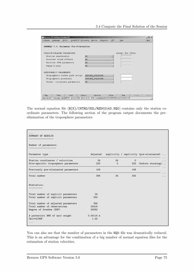
5.4 Compute the Final Solution of the Session
The normal equation file (${K}/INTRO/SOL/RED02143.NQ0) contains only the station co-ordinate parameters. The following section of the program output documents the pre–elimination of the troposphere parameters:
...
SUMMARY OF RESULTS
------------------
Number of parameters:
--------------------
Parameter type Adjusted explicitly / implicitly (pre-eliminated) ...
------------------------------------------------------------------------------------------------ ...
Station coordinates / velocities 24 24 0 ...
Site-specific troposphere parameters 223 0 223 (before stacking)...
------------------------------------------------------------------------------------------------ ...
Previously pre-eliminated parameters 109 109
------------------------------------------------------------------------------------------------ ...
Total number 356 24 332 ...
Statistics:
----------
Total number of explicit parameters 24
Total number of implicit parameters 332
Total number of adjusted parameters 356
Total number of observations 20418
Degree of freedom (DOF) 20062
A posteriori RMS of unit weight 0.00114 m
Chi**2/DOF 1.30
...
You can also see that the number of parameters in the NQ0–file was dramatically reduced.This is an advantage for the combination of a big number of normal equation files for theestimation of station velocities.
Bernese GPS Software Version 5.0 Page 75

5. Terminal Session: Thursday
5.5 Velocity Estimation
The velocity estimation in program ADDNEQ2 is easy. Introduce the normal equation filescontaining only the station coordinate parameters. The normal equation files have to covera reasonable time interval to reliably estimate velocities (in this case one year):
Page 76 AIUB

5.5 Velocity Estimation
Station velocities are set up by marking the checkbox:
Furthermore we check the repeatability of the daily solutions after the velocity estimation.The coordinates in the resulting file will refer to the epoch 2000 01 01.
Bernese GPS Software Version 5.0 Page 77
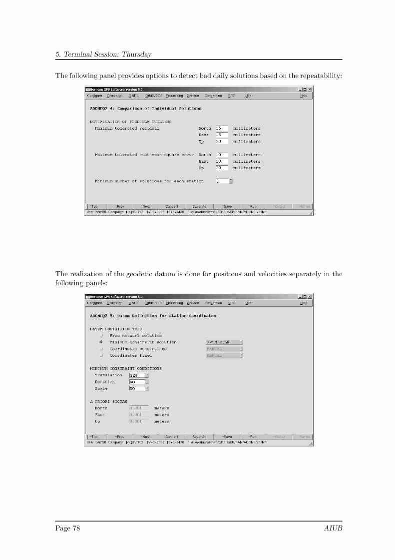
5. Terminal Session: Thursday
The following panel provides options to detect bad daily solutions based on the repeatability:
The realization of the geodetic datum is done for positions and velocities separately in thefollowing panels:
Page 78 AIUB

5.5 Velocity Estimation
Bernese GPS Software Version 5.0 Page 79

5. Terminal Session: Thursday
After the velocity estimation the repeatability of the coordinates solutions from the indi-vidual normal equations looks like:
...
Comparison of Individual Solutions:
----------------------------------
BRUS N 0.59 -0.47 0.47 -0.56 0.52
BRUS E 0.31 -0.29 0.36 0.20 -0.18
BRUS U 1.53 0.62 -0.58 1.80 -1.75
FFMJ N 0.27 -0.32 0.34 0.00 0.02
FFMJ E 0.26 0.33 -0.32 0.01 0.00
FFMJ U 0.95 0.99 -1.14 -0.48 0.44
MATE N 0.03 0.02 0.01 0.04 0.01
MATE E 0.58 -0.32 0.35 -0.64 0.60
MATE U 0.63 -0.61 0.72 -0.35 0.42
ONSA N 0.76 0.19 -0.27 0.90 -0.90
ONSA E 0.38 0.23 -0.25 0.40 -0.39
ONSA U 1.34 -1.04 1.30 -1.10 1.19
PTBB N 0.55 0.29 -0.32 -0.60 0.60
PTBB E 0.16 0.12 -0.11 0.17 -0.16
PTBB U 0.32 -0.49 0.27 0.01 -0.05
VILL N 0.54 -0.33 0.28 -0.60 0.56
VILL E 0.31 0.05 -0.10 0.36 -0.39
VILL U 1.13 -0.90 1.00 -0.98 1.04
ZIMJ N 0.43 0.36 -0.16 0.47 -0.43
ZIMJ E 0.23 -0.19 0.12 -0.23 0.23
ZIMJ U 0.83 0.60 -0.56 0.77 -0.89
ZIMM N 0.44 0.25 -0.34 0.43 -0.46
ZIMM E 0.17 0.17 -0.13 -0.13 0.15
ZIMM U 0.81 0.83 -1.01 0.34 -0.40
Below this table all bad daily solutions according to the settings in panel “ADDNEQ2 4:
Comparison of Individual Solutions” are summarized. if bad daily solution are detected. In thatcase we have no additional section and, therefore, no outliers.
Page 80 AIUB

5.5 Velocity Estimation
If you compare the velocities obtained for the two GPS receivers in Zimmerwald (ZIMJ andZIMM) you will find small differences:
...
Station coordinates and velocities:
----------------------------------
Reference epoch: 2000-01-01 00:00:00
Station name Typ A priori value Estimated value Correction RMS error ...
-------------------------------------------------------------------------------------------- ...
...
ZIMJ 14001M006 VX -0.0129 -0.0156 -0.0027 0.0011
VY 0.0182 0.0175 -0.0007 0.0004
VZ 0.0098 0.0099 0.0001 0.0011
VU 0.0000 -0.0018 -0.0019 0.0015 ...
VN 0.0143 0.0164 0.0021 0.0004 ...
VE 0.0197 0.0194 -0.0003 0.0003 ...
...
ZIMM 14001M004 VX -0.0129 -0.0131 -0.0002 0.0010
VY 0.0182 0.0185 0.0003 0.0004
VZ 0.0098 0.0120 0.0022 0.0011
VU 0.0000 0.0015 0.0015 0.0014 ...
VN 0.0143 0.0159 0.0016 0.0004 ...
VE 0.0197 0.0201 0.0004 0.0003 ...
...
You may constrain the velocity estimates for a pair of sites in the station informationfile. Copy the original station information file ${K}/INTRO/STA/EXAMPLE.STA and add thefollowing line to this copy
TYPE 004: STATION COORDINATES AND VELOCITIES (ADDNEQ)
-----------------------------------------------------
RELATIVE CONSTR. POSITION RELATIVE CONSTR. VELOCITY
STATION NAME 1 STATION NAME 2 NORTH EAST UP NORTH EAST UP
**************** **************** **.***** **.***** **.***** **.***** **.***** **.*****
ZIMM 14001M004 ZIMJ 14001M006 0.00001 0.00001 0.00001
(Pay attention on the number of blank lines before the next section starts.)
Introducing this modified station information file instead of the original one you will getthe following estimates for the station velocities in Zimmerwald:
Bernese GPS Software Version 5.0 Page 81

5. Terminal Session: Thursday
...
Station coordinates and velocities:
----------------------------------
Reference epoch: 2000-01-01 00:00:00
Station name Typ A priori value Estimated value Correction RMS error ...
-------------------------------------------------------------------------------------------- ...
...
ZIMJ 14001M006 VX -0.0129 -0.0143 -0.0014 0.0009
VY 0.0182 0.0181 -0.0001 0.0003
VZ 0.0098 0.0110 0.0012 0.0009
VU 0.0000 -0.0000 -0.0001 0.0012 ...
VN 0.0143 0.0162 0.0019 0.0003 ...
VE 0.0197 0.0198 0.0001 0.0003 ...
...
ZIMM 14001M004 VX -0.0129 -0.0143 -0.0014 0.0009
VY 0.0182 0.0181 -0.0001 0.0003
VZ 0.0098 0.0110 0.0012 0.0009
VU 0.0000 -0.0000 -0.0001 0.0012 ...
VN 0.0143 0.0162 0.0019 0.0003 ...
VE 0.0197 0.0198 0.0001 0.0003 ...
...
The final results are contained in the files ${K}/INTRO/STA/FINAL.CRD
EXAMPLE: Estimate final solution - coordinates and velocities 13-FEB-07 14:59
--------------------------------------------------------------------------------
LOCAL GEODETIC DATUM: IGS00 EPOCH: 2000-01-01 0:00:00
NUM STATION NAME X (M) Y (M) Z (M) FLAG
6 BRUS 13101M004 4027893.8398 307045.7403 4919475.0665 A
15 FFMJ 14279M001 4053455.9388 617729.5767 4869395.6460 A
36 MATE 12734M008 4641949.6604 1393045.3349 4133287.3899 W
42 ONSA 10402M004 3370658.6174 711877.0633 5349786.9038 W
47 PTBB 14234M001 3844060.0446 709661.2309 5023129.5007 A
56 VILL 13406M001 4849833.7491 -335049.1265 4116014.8656 W
63 ZIMJ 14001M006 4331294.0075 567542.0461 4633135.6607 A
64 ZIMM 14001M004 4331297.1406 567555.7889 4633133.8693 A
and ${K}/INTRO/STA/FINAL.VEL
EXAMPLE: Estimate final solution - coordinates and velocities 13-FEB-07 14:59
--------------------------------------------------------------------------------
LOCAL GEODETIC DATUM: IGS00
NUM STATION NAME VX (M/Y) VY (M/Y) VZ (M/Y) FLAG PLATE
6 BRUS 13101M004 -0.0205 0.0173 0.0086 A EURA
15 FFMJ 14279M001 -0.0105 0.0167 0.0104 A EURA
36 MATE 12734M008 -0.0199 0.0184 0.0126 W EURA
42 ONSA 10402M004 -0.0130 0.0156 0.0088 W EURA
47 PTBB 14234M001 -0.0190 0.0167 0.0056 A EURA
56 VILL 13406M001 -0.0096 0.0208 0.0114 W EURA
63 ZIMJ 14001M006 -0.0143 0.0181 0.0110 A EURA
64 ZIMM 14001M004 -0.0143 0.0181 0.0110 A EURA
Page 82 AIUB

5.6 Daily Goals
5.6 Daily Goals
At the end of today’s session, you should have:
(1) used GPSEST to compute a final solution of the day, created files:FIX02143.OUT, FIX02143.NQ0 (for all sessions),
(2) checked the coordinates of the fiducial sites using ADDNEQ2 andHELMR1, created files: FIN02143.CRD,FIN02143.TRP, FIN02143.OUT, andHELMR1.OUT,
(3) used COMPAR to check the daily repeatabilities, created file COMPAR.OUT,
(4) used ADDNEQ2 to create a final session solution, and reduced size NQ0s,created file: RED02143.NQ0 and RED02143.SNX,
(5) if possible, used ADDNEQ2 for velocity estimation, created files: FINAL.CRDand FINAL.VEL.
Bernese GPS Software Version 5.0 Page 83

6. Terminal Session: Friday
In the previous terminal sessions you have estimated coordinates, velocities, andtroposphere parameters. This is the standard application of the Bernese GPS Soft-ware for most users.If you have finished this work you may compute some special solutions todayaccording to your interest. This document provides some suggestions to practice:
• kinematic positioning for a station,
• zero–difference processing to estimate clocks, or
• use of the Bernese Processing Engine.
6.1 Kinematic Positioning
The example campaign contains no really roving stations. You can, however, define one ofthem to be kinematic (e.g., station FFMJ). Introduce the coordinates from the final solution(${K}/INTRO/STA/FIN02143.CRD) for all other sites.
AIUB

6.1 Kinematic Positioning
Store the kinematic coordinates in an output file (“Kinematic coordinates” in panel“GPSEST 2.2: Output Files 2”).
Because the number of parameters for the kinematic positioning may become very large weselect only a short data interval for this kinematic positioning:
Fix all station coordinates apart from FFMJ in the panels “Datum Definitions for Sta-
tions” (choose MANUAL in panel “GPSEST 4” and select all stations except FFMJ in panel“GPSEST 4.2”).
Bernese GPS Software Version 5.0 Page 85

6. Terminal Session: Friday
Enable the kinematic coordinates option without any pre–elimination in a first run:
Let us assume only horizontal movements for this site:
Page 86 AIUB

6.1 Kinematic Positioning
As expected you will get only small estimates for the kinematic coordinates since FFMJwas not moving:
KINEMATIC COORDINATES: ${K}/INTRO/STA/KIN02143.KIN
---------------------
EPO: EPOCHS SINCE 2002-05-23 02:00:00 (SAMPLING 300 SEC)
CORRECTION AND RMS IN METER ...
EPO EPOCH(MJD) #OBS STA LATITUDE LONGITUDE HEIGHT ...
---------------------------------------------------------------------------------------------- ...
FFMJ 14279M001 50 5 26.079483 8 39 53.878597 178.1970
1 52417.083333 21 FFMJ -0.0297 +- 0.011 -0.0170 +- 0.007 -0.0001 +- 0.001 ...
2 52417.086806 21 FFMJ -0.0147 +- 0.009 -0.0047 +- 0.006 -0.0000 +- 0.001 ...
3 52417.090278 22 FFMJ -0.0040 +- 0.009 -0.0058 +- 0.006 0.0002 +- 0.001 ...
4 52417.093750 23 FFMJ -0.0020 +- 0.010 -0.0054 +- 0.007 -0.0001 +- 0.001 ...
5 52417.097222 23 FFMJ -0.0048 +- 0.012 -0.0014 +- 0.009 -0.0000 +- 0.001 ...
Further suggestions:
• Introduce the result file with kinematic coordinates as an input file for another run ofGPSEST. If the estimates become zero it is a confirmation that the file was correctlyconsidered as the a priori kinematic positions for the station FFMJ.
• Use the pre–elimination EVERY EPOCH for the “Kinematic coordinates” (they are back–substituded by the program in order to get a solution also for those parameters).Compare the results with the first solution.
• Switch the “Var–covar wrt epoch parameters” in panel “GPSEST 3.2: General Options 2” fromSIMPLIFIED to CORRECT. Compare the results again with the first solution.
• Compute kinematic coordinates for the full day using the epoch–wise pre–eliminationand back–substitution algorithm. To save computing power we recommend to samplethe data to 300 s.
• You may also run the pre–processing programs CODSPP and MAUPRP for “kinematicstations”.
In addition you may use the Bernese GPS Software with zero–difference observations toobtain kinematic positions. Smoothed code, phase–only, or combined code and phase solu-tions are possible. Consult the following section on clock estimation for the preprocessing ofzero–difference data. Compare the results you generate with the different observation typesto get an impression on the accuracy that can be obtained.
Bernese GPS Software Version 5.0 Page 87

6. Terminal Session: Friday
6.2 Clock Estimation
For the clock estimation we have to use code and phase data together. The data are analyzedat zero–difference level.
The preprocessing for zero–difference data starts with program RNXSMT, available in ”Menu
>RINEX>RINEX utilities>Clean/smooth observation files”. In the first panel select all RINEX files of asession. The default input options perform well in most cases:
In order to import the smoothed RINEX observation files into the Bernese format you haveto select them in the first input panel of program RXOBV3 (note that you will overwriteyour zero–difference observation files from the previous processing example by doing this):
Page 88 AIUB

6.2 Clock Estimation
Because we want to compute clock values with a sampling of 5 min. only in GPSEST you canresample the observations already in RXOBV3: set the “Sampling interval” in panel “RXOBV3 2:
Input Options 1” to 300 seconds.
Furthermore you have to consider the “SIGNAL STRENGTH REQUIREMENTS” for smoothedRINEX files (see online help):
After importing the data into the Bernese format you have to repeat the receiver clocksynchronization with program CODSPP. The options are identical to the settings in Sec-tion 3.3.1. The only difference is that we select CODE for the option “Mark outliers in obs.
Bernese GPS Software Version 5.0 Page 89

6. Terminal Session: Friday
files” in the last input panel. In this way very bad code observations are excluded from theparameter estimation in program GPSEST.
Now you are ready to run GPSEST in the zero–difference mode. Introduce the estimatedcoordinates and troposphere parameters from the final solution you have computed for thesession:
Page 90 AIUB

6.2 Clock Estimation
Bernese GPS Software Version 5.0 Page 91

6. Terminal Session: Friday
Page 92 AIUB

6.2 Clock Estimation
The residuals are stored in the file ${K}/INTRO/OUT/CLK02143.RES. Use program RESRMSto screen for outliers bigger than 2 cm for code and phase data (remember that code residualsare scaled to phase residuals — 2 cm in the input field correspond to a 2 m threshold forcode residuals):
Mark the corresponding observations using program SATMRK and repeat the GPSEST–run. In the second iteration we screen for residuals bigger than 6 mm in RESRMS andmark these observations with SATMRK, too. Repeat the run of GPSEST a third time to getthe definitive clock estimates. Specify a “Clock RINEX” file (e.g., CLK$YD+0) in the panel“GPSEST 2.1: Output Files 1”.The clock solution is finalized by selecting the reference clock using program CCRNXC (”Menu
>RINEX>RINEX utilities>Combine/manipulate clock data”):
Bernese GPS Software Version 5.0 Page 93
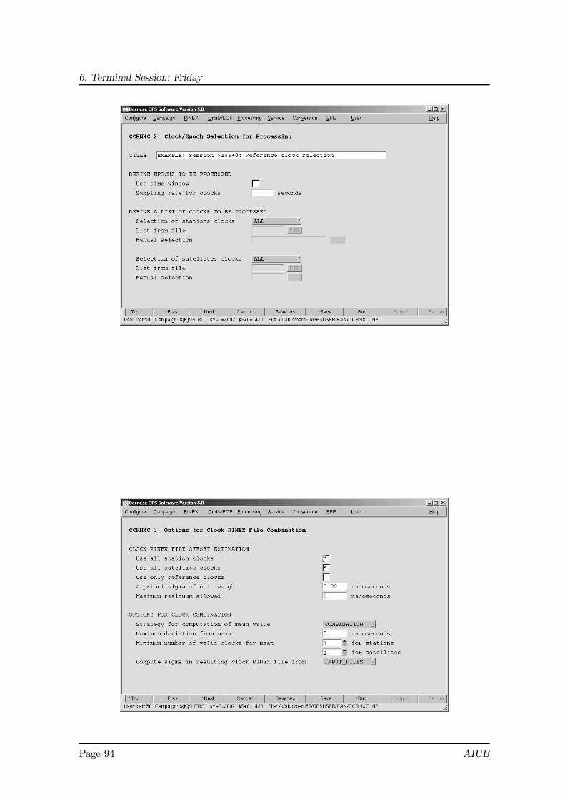
6. Terminal Session: Friday
Page 94 AIUB

6.2 Clock Estimation
Bernese GPS Software Version 5.0 Page 95

6. Terminal Session: Friday
The table at the end of the program output provides an overview of the clock quality:
...
REFERENCE CLOCK SELECTION FOR OUTPUT FILE
----------------------------------------------------------------------------------
Selected reference station: MATE 12734M008
...
STATISTICS ON THE CLOCKS IN THE OUTPUT FILE
-------------------------------------------
# per file rms of poly. fit (ns)
Clock name out 001 n = 0 n = 1 n = 2
-------------------------------------------------------------------
MATE 12734M008 288 288 57.543 0.000 0.000
ONSA 10402M004 288 288 36.041 0.100 0.093
PTBB 14234M001 288 288 1.222 0.138 0.072
BRUS 13101M004 278 278 2.497 1.600 1.358
VILL 13406M001 288 288 24.142 23.310 18.686
FFMJ 14279M001 281 281 0.3E+06 0.3E+06 0.3E+06
ZIMJ 14001M006 169 169 0.3E+06 0.3E+06 0.3E+06
ZIMM 14001M004 288 288 0.3E+06 0.3E+06 0.3E+06
G20 80 80 19.792 0.161 0.161
G14 106 106 52.600 0.183 0.154
...
Further suggestions:
• Use the PPP approach to screen the residuals of the Bernese zero–difference observa-tion files. This has to be done station by station. Make sure that you use a consistentset of orbits, EOP, and satellite clocks (e.g., final IGS products or final CODE solu-tion).
• Switch the “Var–covar wrt epoch parameters” in panel “GPSEST 3.2: General Options 2” fromSIMPLIFIED to CORRECT.
• Make a PPP for one of the stations included in the network and compare the obtainedclock corrections with the estimates from the network solution generated before. Youmay either use the IGS clocks (extract the satellite clocks from the clock RINEX filesin the OUT–directory of your campaign using the program CCRNXC) or the satelliteclock estimates from your network solution (specify a “Bernese satellite clock file” in the“RESULT FILES” section of the panel “CCRNXC 1: Filenames”).
6.3 Bernese Processing Engine
It is possible to run one of the example BPEs provided with the distribution. They areinstalled in your user environment and the data are available, too. In detail these are:
(1) PPP.PCF — Precise Point Positioning
(2) RNX2SNX.PCF — Generate a SINEX file starting with GNSS RINEX observation files
(3) CLKDET.PCF — Estimate station and satellite clocks
Page 96 AIUB

6.3 Bernese Processing Engine
The reference files for the solution are also available in your campaign directories.
Be aware that some of the files you have generated in the previous terminal sessions maybe overwritten.
Even if it is simple to run a BPE: please, do not run all BPEs for all sessions. First it israther boring to look at the screen with a BPE running and, secondly, we like to avoid tooverload the CPUs. Running one example for one session with the BPE should be enoughto get the BPE output files.
Select first the session for which you want to run the BPE (e.g., day 143 of year 2002). Tostart the BPE use ”Menu>BPE>Start BPE process”:
Bernese GPS Software Version 5.0 Page 97

6. Terminal Session: Friday
In addition we suggest to become familiar with the structure and the functionality of theBPE in this terminal session, e.g.,
• by reading the header information of the PCF files,
• by viewing the user scripts of the example BPE that can be used as modules for yourown BPE at home, or
• by studying the BPE output files.
Page 98 AIUB