bernoulli bandits an empirical comparison - ucl/elen · bernoulli bandits an empirical comparison...

Bernoulli BanditsAn Empirical Comparison

Ronoh K.N1,2, Oyamo R.1,2, Milgo E.1,2, Drugan M.1 and Manderick B.1

1- Vrije Universiteit Brussel - Computer Sciences Department - AI LabPleinlaan 2 - B-1050 Brussels - Belgium

2- Moi UniversityP.o - Box - 3900- 30100 - Eldoret - Kenya

Abstract. An empirical comparative study is made of a sample ofaction selection policies on a test suite of the Bernoulli multi-armed banditwith K = 10, K = 20 and K = 50 arms, each for which we considerseveral success probabilities. For such problems the rewards are eitherSuccess or Failure with unknown success rate. Our study focusses on ε-greedy, UCB1-Tuned, Thompson sampling, the Gittin’s index policy, theknowledge gradient and a new hybrid algorithm. The last two are not well-known in computer science. In this paper, we examine policy dependenceon the horizon and report results which suggest that a new hybridizedprocedure based on Thompsons sampling improves on its regret.

1 Introduction

In this paper, we compare empirically a number of action selection policies on aspecial case of the stochastic multi-armed bandit (MAB) problem: the Bernoullibandit. The bandit does not know the expectations of the reward distributions.In order to estimate them, the rewards have to be collected from all arms. Eachtime a new reward is obtained, the estimate of the corresponding distribution isupdated and the agent becomes more confident in the new estimate. Meanwhile,the agent has to try to achieve its goal: maximising the total expected reward.The MAB, introduced by [1], is the simplest example of a sequential decisionproblem where the agent has to find a proper balance between exploitation andexploration. The importance of the MAB lies in the exploitation-explorationtradeoff inherent in sequential decision making. Exploitation means that thegreedy arm is selected, i.e. the one with the highest observed average reward.Since this is not necessarily the optimal arm, the agent may resolve to explorationof a non-greedy arm to improve the estimate of its expected reward. An actionselection policy tells the agent which arm to pull next. Regret is the expectedloss after n time steps due to the fact that it is not always the optimal arm thatis played. Maximizing the total expected reward is equivalent to minimizingthe total expected regret. The expected regret incurred after n time steps isdefined as R(n) , nµ∗ −

∑ni=1 µn, where µ∗ is the largest true mean and µn

is the true mean of the arm pulled at time step n. This can be rewritten asR(n) = nµ∗ −

∑Kk=1 µk E(nk), where E(nk) is the expected number of times

that arm k is played during the first n time steps. MAB-problems can beclassified according to reward distributions of the arms, the time horizon which is

59

ESANN 2015 proceedings, European Symposium on Artificial Neural Networks, Computational Intelligence and Machine Learning. Bruges (Belgium), 22-24 April 2015, i6doc.com publ., ISBN 978-287587014-8. Available from http://www.i6doc.com/en/.

finite or infinite, and statistical analysis are usually either done according to thefrequentist or the Bayesian paradigm. Theoretical studies prefer to minimize thetotal expected regret or loss. Since theory only gives worst case upper bounds forthe this regret. The empirical performance of a policy is in most cases better thanindicated by these theoretical regret bounds. Moreover, for many action selectionpolicies there is no theoretical analysis. The rest of this paper is organised asfollows: In Section 2, we give a brief review of previous empirical research.Section 3 gives the basics of the Bernoulli bandit problem. Section 4, reviewsthe action selection policies considered in the empirical comparison. Section 5describes the experimental setup and the results. Finally, the conclusion is givenin Section 6.

2 State of the Art of Empirical Comparison

A systematic evaluation by [2] compared popular action-selection policies usedin reinforcement learning but did not include the Gittins index, the knowledgegradient and Thompson sampling. It investigated the effect of the variance ofrewards on the policy’s performance and optimally tuned the parameters of eachone. Another paper [3] gave a preliminary study of ε-greedy with softmax andinterval estimation. Unfortunately, it did not detail performance measures used,hence the difficulty in interpretation of results. This study gives an insight intothe ε-greedy (εG), used successfully in reinforcement learning, the UCB1-Tuned,a variant of the upper confidence bound (UCB) policies that works very well inpractice, the Gittins index (GI) and the knowledge gradient (KG) relative toThompson sampling (TS), a Bayesian approach to the exploitation-explorationtrade-off that recently became popular in machine learning. TS has been shownto provide the best alternative for MABs with side observations and delayedfeedback. The policy is broadly applicable and easy to implement [4]. GI andKG are quite popular in operations research but are they relatively unknownin the machine learning community. The motivation for our empirical compar-ison is threefold: few empirical comparisons have been done so far, theoreticalcomparison is still limited in its scope in some cases, and an empirical under-standing of the Bernoulli bandit problem is important for many applications,e.g. optimizing the click through rate [5].

3 Bernoulli Bandit

In the Bernoulli bandit problem, the agent chooses among K different arms:k = 1, · · · ,K. When arm k is pulled either the reward 1 for Success is receivedwith probability µk or 0 for Failure with probability 1 − µk. The rewards thushave a Bernoulli distribution Ber(µk) with unknown success probability µk. Theestimated mean after nk trials, of which sk are successes and fk are failures, isgiven by µ̂k = sk

sk+fk. The optimal arm k∗ = arg max1≤k≤K µk is the one with

the highest true but unknown mean µ∗ = max1≤k≤K µk. It is always assumedthat the arms are sorted according to their expected rewards: µ1 > · · · > µk >

60


· · · > µK , i.e. the first arm is the optimal one and the last is the worst one. Foreach non-optimal arm, i.e. k 6= 1, the optimality gap is defined as ∆k , µ∗−µk

and the smallest gap ∆ , mink 6=1 ∆k is assumed to be positive so that not morethan one arm is optimal. The greedy arm at each time step is the arm with thehighest estimated mean at that moment: k̂∗ = arg max1≤k≤K µ̂k. The greedyarm might be different from the optimal one, especially in the beginning whentoo few rewards are available to have a reliable estimate of the true means.

4 Brief Description of the Action - Selection Policies

The ε-Greedy (εG) selects the greedy arm k̂∗ most of the time with probability1 − ε (exploitation), while with a small probability ε it selects uniformly atrandom one of the K arms regardless of their estimated mean (exploration) [6].εG works well in practice and is considered to be a benchmark.

Thompson Sampling (TS) relies on the presence and analysis of posteriordata [7]. It maintains a prior distribution for the unknown parameters whichat each time step n, when an arm has been played and a reward obtained, isupdated using Bayes’ rule to obtain the posterior. The arm with the probabilityof being the most optimal according to the current posterior distributions is thenpulled. Reward samples are taken from the distribution and the best arm playedaccording to the drawn parameters. TS can be summarized as follows [5]:

Algorithm 1 Thompson SamplingInput: Initial number of successes sk = 0, the failures fk = 0, and their sumnk = 0for timestep n = 1, · · · , N do

1. For each k = 1, · · · ,K, sample rk from the corresponding distributionBeta(sk, fk)

2. Play arm k∗ = arg maxk rk and receive reward r

3. If r = 1, increment sk∗ else increment fk∗

The UCB1-Tuned belongs to the class of Upper Confidence Bound (UCB)policies that compute an index to decide deterministically which arm to pull.UCB-policies are examples of optimism in the face of uncertainty [8]. The agentmakes optimistic guesses about the expected rewards of the arms and selects thearm with the highest guess. UCB1-Tuned is a variant that has a finite-time regretlogarithmically bound for arbitrary sets of reward distributions with boundedsupport. It takes the estimated variance Vk when arm k is pulled nk into accountand can be summarized as follows [6]:

61


Algorithm 2 UCB1-TunedInput: Initial rk = 0for timestep n = 1, · · · , N do

1. Play machine k that maximizes r̄k +√

ln nnk

min(1/4, Vk(nk)), where r̄k isthe estimated mean reward of arm k, and update r̄k with the obtainedreward rk

We have included TSH which is a hybrid that starts as UCB1-Tuned whichhas better initial performance and continues as TS which outperforms UCB1-Tuned after some time. The switching time is determined empirically and in-creases as the number of arms increases.

The Gittins index νG of an arm depends on the number of times nk it hasbeen selected. GI relates the problem of finding the optimal policy to a stoppingtime problem [9]. It determines for each arm an index νG and selects at eachtime the arm with the highest value.

Algorithm 3 Finite Horizon Gittins for Bernoulli BanditsInput: Initial successes sk = 0, failures fk = 0, and their sum nk = 0.for each time step n = 1, · · · , N , do

1. Play each arm once and calculate its FHG-index νG(sk, fk)

2. Play arm k∗ = arg maxk νG(sk, fk) and observe corresponding reward r.In case of ties, choose one arm randomly among them.

3. If r = 1, increment sk∗ else increment fk∗ and recalculate indexνG(sk∗ , fk∗) of arm k∗.

The Knowledge Gradient (KG) can be adapted to handle cases where therewards of the arms are correlated [10]. The policy selects an arm accordingto: kKG = arg max1≤k≤K µ̂k + (N − n)νKG(k) where νKG(k) is the knowledgegradient index of arm k. KG adopts the procedure that follows:

62


Algorithm 4 Finite Horizon Knowledge Gradient for Bernoulli BanditsInput: Initial sk = 0, fk = 0 and nk = sk + fk

for k = 0, 1, · · · ,K and n = 1, · · · , N do

1. Calculate the KG-index ν(k)KG(sk, fk)

2. Play arm k∗ = arg maxk νKG(sk, fk) and observe corresponding reward r.In case of ties, choose one arm randomly among them.

3. If r = 1, increment sk∗ else increment fk∗ and recalculate indexνKG(sk∗ , fk∗) of arm k∗.

5 Empirical Analysis

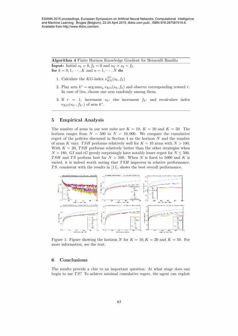
The number of arms in our test suite are K = 10, K = 20 and K = 50. Thehorizon ranges from N = 500 to N = 10, 000. We compare the cumulativeregret of the policies discussed in Section 4 as the horizon N and the numberof arms K vary. TSH performs relatively well for K = 10 arms with N > 100.With K = 20, TSH performs relatively better than the other strategies whenN > 180. GI and εG greedy surprisingly have notably lesser regret for N ≤ 500.TSH and TS perform best for N > 500. When N is fixed to 5000 and K isvaried, it is indeed worth noting that TSH improves in relative performance.TS, consistent with the results in [11], shows the best overall performance.

Figure 1: Figure showing the horizon N for K = 10,K = 20 and K = 50. Formore information, see the text.

6 Conclusions

The results provide a clue to an important question: At what stage does onebegin to use TS? To achieve minimal cumulative regret, the agent can exploit

63


the theoretical guarantees of the UCB1-Tuned before using TS. Further empir-ical studies should ascertain the time needed to initialize deterministically. Thepossibility of a policy incorporating the features of UCB and TS to minimizecumulative regret needs to be investigated. The analysis was done for an envi-ronment for which the success rate was fixed - empirical tests need to be donefor scenarios where the rates change according to some stochastic process.

References

[1] H. Robbins. Some aspects of the sequential design of experiments. Bulletinof the American Mathematical Society, 58(5):527–535, 1952.

[2] Volodymyr Kuleshov and Doina Precup. Algorithms for the multi armedbandit problem. Journal of Machine Learning, 1, PP. 1 - 48, 2000.

[3] Joannes Vermorel and Mehryar Mohri. Multi armed bandit algorithmsand empirical evaluation. In European Conference on Machine Learning,Springer, PP. 437-448, 2005.

[4] Shie Manor Aditya Gopalan and Yishay Mansour. Thompsons sampling forcomplex online problems. Proceedings of the 31st International Conferenceon Machine Learning, Beijing, China, W and CP Vol. 32, 2014.

[5] Olivier Chapelle and Lihong Li. An empirical evaluation of thompsonssampling. Yahoo! Research,Santa Clara Canada, CA, NIPS 2011: 2249-2257, 2011.

[6] C. Nicolo P. Auer and P. Fischer. Finite-time analysis of the multiarmedbandit problem. Machine Learning, Kluwer Academic Publishers., Vol.. 47:235-256, 2002.

[7] Thompsons W.R. On the likelihood that one unknown probability exceedsanother in view of evidence of two samples. Biometrika, 01/1933, 25: 285-294, 1933.

[8] S. Bubeck and N. Cesa-Bianchi. Regret analysis of stochastic and non-stochastic multi-armed bandit problems. Foundations and Trends in Ma-chine Learning, 5(1):1–122, 2012.

[9] K. Glazebrook J. C. Gittins and R. Weber. Multi-Armed Bandit AllocationIndices. J. Wiley And Sons, Series Wiley-Interscience Series In SystemsAnd Optimization, New York, 2011.

[10] W. B. Powell and I. O. Ryzhov. Optimal Learning. John Wiley and Sons,Canada, 2012.

[11] Shipra Agrawal and Navil Goyan. Analysis of thompsons sampling for themulti-armed bandit problem. JMLR: Workshop and Conference Proceed-ings, 23:39.1- 39.26, 2012.

64


bernoulli bandits an empirical comparison - ucl/elen · bernoulli bandits an empirical comparison...

Documents