bessel beams: a novel approach to periodic structures · bessel beams: a novel approach to periodic...
TRANSCRIPT
Imperial College London
Imperial College London
The Blackett Laboratory
Photonics Group
Bessel Beams: A Novel Approach
to Periodic Structures
Andrew W. G. Norfolk
Thesis submitted in partial fulfilment of the requirements for the
degree of Doctor of Philosophy of Imperial College London.
September 21, 2010

2

For my Mum and Dad
and
in memory of my uncle Richard
who first inspired me to study at Imperial College London.
3

4
Acknowledgements
First and foremost I would like to thank my supervisors Edward Grace and Martin McCall
for giving me this opportunity to do this PhD and their help, encouragement and words
of wisdom throughout. A PhD is not without its difficulties and I am grateful that Ed has
never let me struggle alone and pushed me to work hard and to the best of my ability when
it really mattered. His unyielding enthusiasm has helped keep me motivated throughout
my PhD. I am doubtless that without his contribution this would have been a dull and
uneventful experience.
I would also like to acknowledge and thank Alberto for his near encyclopedic knowledge
of all things mathematical and for his help understanding critical self-focusing.
Writing up is a tough business and it was excellent to go through this with two excellent
friends Pete and Simon. Pete, the archetypal ENTP, always willing to argue on any subject
and never shy of a swift drink after a long day’s work and Simon, who repeatedly amused
us all with the mother of all puns, have kept me grounded during my time writing up.
I would like to thank Andrew “K-dawg” Kao for his insightful discussions over many a
chilled beverage.
All work and no play would have made Andrew a very dull boy! To that end I would
like to thank my friends in the Photonics group. To Ara, Dom, Dan and the rest of the
Dam-lab crew for a fantastic welcome to the Photonics social scene. An honorable mention
should go to Gabs and Mike for their ‘loveable rudeness’ and for brightening up tea breaks.
Hannah for her continuous and unconditional love, support and sympathy throughout
my PhD and keeping out of trouble while I wrote up. Finally to my family; Jess, for the
wavering support only a little sister can provide, and my parents, without whom none of
this would have been possible, who have always believed in my goals and supported me
wholeheartedly throughout my whole life, words cannot express how grateful I am for this.
5

ACKNOWLEDGEMENTS
6

Declaration
All the work presented in this thesis is my own and any additional contributions are
acknowledged or referenced where appropriate.
7

ACKNOWLEDGEMENTS
8

Abstract
Bessel and Bessel-like beams in Kerr-like nonlinear materials are numerically investi-
gated. This is conducted with a view to exploiting the behaviour of such profiles for the
direct laser writing of periodic structures in highly nonlinear glasses. A highly efficient
numerical model is developed for the propagation of radially symmetric profiles based on
the quasi-discrete Hankel transform (QDHT), making use of a reconstruction relation to
allow the field to be sampled at arbitrary positions that do not coincide with the numerical
grid. This Hankel-based Adaptive Radial Propagator (HARP) is shown to be up to 1000
times faster than standard FFT-based methods.
The critical self-focusing of the Gaussian beam is reproduced to confirm the accuracy
of HARP. Following this the critical self-focusing behaviour of a Bessel-Gauss beam is
investigated. It is observed that, for certain parameters, increasing the beam power may
prevent blowup in the Bessel-Gauss beam.
Below the threshold for self-focusing the Bessel-Gauss beam exhibits periodic modu-
lation in the direction of propagation. The existing equation describing this behaviour
is shown to be inaccurate and a modification is proposed based on a power dependent
beat-length. This modified beat-length equation is demonstrated to be accurate in both
the paraxial and quasi-nonparaxial regime. As the beam decays, the intensity modulation
appears negatively chirped. It is demonstrated that this chirp may be controlled through
careful shaping of the window. It is also shown that a small Gaussian seed beam may be
used to control the positions of the maxima.
It is demonstrated that a set of nonlinear Bessel functions exist that exhibit a similar
quasi-stationary behaviour in a nonlinear medium to the linear Bessel beam in a linear
medium. Furthermore it is shown for the first time that higher-order, Bessel-like, station-
ary solutions exist for beams with azimuthal phase, and boundary conditions for these
functions are derived.
9

10

Nomenclature
Wherever possible a consistent style has been maintained throughout this thesis in keeping
with common literature. A list of commonly used constants, variables and functions is
given on page 13.
Scaled co-ordinates are marked with the tilde (r) up until the end of Section 2.3
whereafter the tilde is suppressed and it is assumed that all co-ordinates (x, y, z, r, θ etc)
are subject to the normalisations given in 2.3 unless explicitly stated otherwise.
Vectors are given in bold face, for example the position vector r, and tensors are called
out explicitly in the text. All operators, with the exception of the Laplace operator, are
given the caret, for example the split-step operator Ass. The complex number,√−1, is
denoted by i.
The Fourier transform of a function f(x) is expressed as F {f(x)} = F (kx) where kx
is the spatial frequency. In the event where the destination co-ordinate system may be
ambiguous it may be stated explicitly as F {f(x)} (kr) = F (kr). The radially symmetric
analogue of the Fourier transform is the Hankel transform for order n given byHn {f(r)} =
F (kr).
11

12

List of variables
Variable Meaning
x, y, z Cartesian co-ordinates
r, φ, z Cylindrical co-ordinates
r Transverse position vector
∇2 Laplace operator
∇2⊥ Transverse Laplace operator
κ Nonparaxiality constant (Section 2.3)
H{f(x)} Hankel transform
F {f(x)} Fourier transform
∂xf(x) Partial derivative of f(x) with respect to x
n0 Linear refractive index
n2 Nonlinear refractive index
k Wavenumber in material
L Linear split-step operator
N Nonlinear split-step operator
m Super Gaussian ‘order’
n Hankel transform order
Jn nth order Bessel function
k0r Bessel beam principal transverse spatial frequency
θ Bessel beam inner cone angle
w0 Bessel-Gauss beam waist size
wg Gaussian beam waist size
13

LIST OF VARIABLES
14

Contents
Acknowledgements 5
Abstract 9
Nomenclature 11
List of variables 13
Contents 15
List of figures 21
List of tables 25
1 Introduction 27
1.1 Integrated optical structures . . . . . . . . . . . . . . . . . . . . . . . . . . . 27
1.1.1 Device Fabrication . . . . . . . . . . . . . . . . . . . . . . . . . . . . 28
1.1.2 Direct Laser Writing . . . . . . . . . . . . . . . . . . . . . . . . . . . 28
1.1.3 3D integrated devices . . . . . . . . . . . . . . . . . . . . . . . . . . 29
1.1.4 Heavy metal oxide glass . . . . . . . . . . . . . . . . . . . . . . . . . 30
1.1.5 Writing techniques . . . . . . . . . . . . . . . . . . . . . . . . . . . . 31
1.2 The Bessel beam . . . . . . . . . . . . . . . . . . . . . . . . . . . . . . . . . 32
1.2.1 Derivation . . . . . . . . . . . . . . . . . . . . . . . . . . . . . . . . . 33
1.2.2 Physical generation . . . . . . . . . . . . . . . . . . . . . . . . . . . . 33
1.2.3 Numerical description . . . . . . . . . . . . . . . . . . . . . . . . . . 36
1.2.4 Other non-diffracting beams . . . . . . . . . . . . . . . . . . . . . . . 37
1.3 Thesis Overview . . . . . . . . . . . . . . . . . . . . . . . . . . . . . . . . . 38
15

CONTENTS
1.3.1 Chapter 2 . . . . . . . . . . . . . . . . . . . . . . . . . . . . . . . . . 38
1.3.2 Chapter 3 . . . . . . . . . . . . . . . . . . . . . . . . . . . . . . . . . 38
1.3.3 Chapter 4 . . . . . . . . . . . . . . . . . . . . . . . . . . . . . . . . . 39
1.3.4 Chapter 5 . . . . . . . . . . . . . . . . . . . . . . . . . . . . . . . . . 39
1.3.5 Chapter 6 . . . . . . . . . . . . . . . . . . . . . . . . . . . . . . . . . 40
2 Understanding self-focusing 41
2.1 The nonlinear refractive index . . . . . . . . . . . . . . . . . . . . . . . . . . 41
2.2 Critical self-focusing . . . . . . . . . . . . . . . . . . . . . . . . . . . . . . . 43
2.3 A nonlinear wave equation . . . . . . . . . . . . . . . . . . . . . . . . . . . . 44
2.3.1 The nonlinear Schrodinger equation . . . . . . . . . . . . . . . . . . 46
2.4 Finite difference modelling . . . . . . . . . . . . . . . . . . . . . . . . . . . 48
2.4.1 Finite difference operators . . . . . . . . . . . . . . . . . . . . . . . . 49
2.4.2 Numerical methods . . . . . . . . . . . . . . . . . . . . . . . . . . . . 50
2.5 Pseudo spectral methods . . . . . . . . . . . . . . . . . . . . . . . . . . . . . 52
2.5.1 Hybrid methods . . . . . . . . . . . . . . . . . . . . . . . . . . . . . 52
2.5.2 Split-step methods . . . . . . . . . . . . . . . . . . . . . . . . . . . . 53
2.6 Nonparaxial modelling . . . . . . . . . . . . . . . . . . . . . . . . . . . . . . 55
2.6.1 Nonparaxial split-step . . . . . . . . . . . . . . . . . . . . . . . . . . 55
2.6.2 Difference differential method . . . . . . . . . . . . . . . . . . . . . . 56
2.6.3 Full volume modelling . . . . . . . . . . . . . . . . . . . . . . . . . . 57
2.7 Conclusions . . . . . . . . . . . . . . . . . . . . . . . . . . . . . . . . . . . . 58
3 Hankel-Based Adaptive Radial Propagator 59
3.1 Chapter introduction . . . . . . . . . . . . . . . . . . . . . . . . . . . . . . . 59
3.2 Radially symmetric propagation methods . . . . . . . . . . . . . . . . . . . 59
3.2.1 Split-step method . . . . . . . . . . . . . . . . . . . . . . . . . . . . 61
3.2.2 Difference Differential Method . . . . . . . . . . . . . . . . . . . . . 62
3.2.3 Optimisation . . . . . . . . . . . . . . . . . . . . . . . . . . . . . . . 63
3.3 Reconstruction . . . . . . . . . . . . . . . . . . . . . . . . . . . . . . . . . . 63
3.3.1 Theory . . . . . . . . . . . . . . . . . . . . . . . . . . . . . . . . . . 65
3.3.2 Analysis . . . . . . . . . . . . . . . . . . . . . . . . . . . . . . . . . . 67
3.4 Adaptive Step Length . . . . . . . . . . . . . . . . . . . . . . . . . . . . . . 71
16

CONTENTS
3.4.1 Theory . . . . . . . . . . . . . . . . . . . . . . . . . . . . . . . . . . 71
3.4.2 Implementation . . . . . . . . . . . . . . . . . . . . . . . . . . . . . . 71
3.4.3 Increased accuracy . . . . . . . . . . . . . . . . . . . . . . . . . . . . 74
3.4.4 Speed . . . . . . . . . . . . . . . . . . . . . . . . . . . . . . . . . . . 75
3.5 Adaptive Grid Size . . . . . . . . . . . . . . . . . . . . . . . . . . . . . . . . 75
3.5.1 Resizing in the QDHT . . . . . . . . . . . . . . . . . . . . . . . . . . 76
3.5.2 Shrinking the grid . . . . . . . . . . . . . . . . . . . . . . . . . . . . 78
3.6 Analysis and applications . . . . . . . . . . . . . . . . . . . . . . . . . . . . 78
3.7 Conclusion . . . . . . . . . . . . . . . . . . . . . . . . . . . . . . . . . . . . 80
4 Critical self-focusing 83
4.1 Self-focusing . . . . . . . . . . . . . . . . . . . . . . . . . . . . . . . . . . . . 83
4.1.1 Catagorising self-focusing . . . . . . . . . . . . . . . . . . . . . . . . 84
4.1.2 Invariants . . . . . . . . . . . . . . . . . . . . . . . . . . . . . . . . . 85
4.1.3 Townes soliton . . . . . . . . . . . . . . . . . . . . . . . . . . . . . . 85
4.2 Predicting the beam fate . . . . . . . . . . . . . . . . . . . . . . . . . . . . . 86
4.2.1 Collapse power . . . . . . . . . . . . . . . . . . . . . . . . . . . . . . 87
4.2.2 Summary of known conditions . . . . . . . . . . . . . . . . . . . . . 88
4.3 Numerically determining the beam fate . . . . . . . . . . . . . . . . . . . . 88
4.4 The modified Townes profile . . . . . . . . . . . . . . . . . . . . . . . . . . . 90
4.5 The Gaussian beam revisited . . . . . . . . . . . . . . . . . . . . . . . . . . 90
4.5.1 Numerical results . . . . . . . . . . . . . . . . . . . . . . . . . . . . . 94
4.6 Bessel-Gauss beam . . . . . . . . . . . . . . . . . . . . . . . . . . . . . . . . 95
4.6.1 Sufficient conditions . . . . . . . . . . . . . . . . . . . . . . . . . . . 95
4.6.2 Numerical Results . . . . . . . . . . . . . . . . . . . . . . . . . . . . 97
4.7 Conclusions . . . . . . . . . . . . . . . . . . . . . . . . . . . . . . . . . . . . 101
5 Zero Order Bessel Beams in Kerr-like Media 103
5.1 The initial Bessel-Gauss beam . . . . . . . . . . . . . . . . . . . . . . . . . . 104
5.1.1 Conversion into real units . . . . . . . . . . . . . . . . . . . . . . . . 104
5.2 Preliminary numerical investigation . . . . . . . . . . . . . . . . . . . . . . . 105
5.3 Frequency space representation . . . . . . . . . . . . . . . . . . . . . . . . . 105
5.3.1 Strong nonlinearity . . . . . . . . . . . . . . . . . . . . . . . . . . . . 105
17

CONTENTS
5.3.2 Weak nonlinearity . . . . . . . . . . . . . . . . . . . . . . . . . . . . 109
5.3.3 Comparison with numerical examples . . . . . . . . . . . . . . . . . 113
5.4 Low power beat length equation . . . . . . . . . . . . . . . . . . . . . . . . 114
5.5 Increasing power . . . . . . . . . . . . . . . . . . . . . . . . . . . . . . . . . 116
5.5.1 Average intensity and Modulation depth . . . . . . . . . . . . . . . . 116
5.5.2 Modulation depth variation with power . . . . . . . . . . . . . . . . 117
5.5.3 Deviation from the beat-length . . . . . . . . . . . . . . . . . . . . . 118
5.5.4 Improving the approximation . . . . . . . . . . . . . . . . . . . . . . 120
5.5.5 Correcting the beat length . . . . . . . . . . . . . . . . . . . . . . . . 120
5.5.6 Super Gaussian windows . . . . . . . . . . . . . . . . . . . . . . . . . 122
5.6 Axial modulation chirp . . . . . . . . . . . . . . . . . . . . . . . . . . . . . . 123
5.6.1 Accurately measuring the beat-length . . . . . . . . . . . . . . . . . 123
5.7 Analysis of chirp . . . . . . . . . . . . . . . . . . . . . . . . . . . . . . . . . 127
5.7.1 Exploiting chirp . . . . . . . . . . . . . . . . . . . . . . . . . . . . . 128
5.8 Propagation through full focus . . . . . . . . . . . . . . . . . . . . . . . . . 129
5.8.1 Beam blowup . . . . . . . . . . . . . . . . . . . . . . . . . . . . . . . 129
5.8.2 Intensity modulation . . . . . . . . . . . . . . . . . . . . . . . . . . . 130
5.8.3 Modulation length . . . . . . . . . . . . . . . . . . . . . . . . . . . . 131
5.8.4 Further work . . . . . . . . . . . . . . . . . . . . . . . . . . . . . . . 133
5.9 Seeding with a Gaussian . . . . . . . . . . . . . . . . . . . . . . . . . . . . . 133
5.9.1 Beam blow-up . . . . . . . . . . . . . . . . . . . . . . . . . . . . . . 135
5.9.2 Numerical results . . . . . . . . . . . . . . . . . . . . . . . . . . . . . 136
5.10 Seeding through full focus . . . . . . . . . . . . . . . . . . . . . . . . . . . . 138
5.11 Nonparaxial Beams . . . . . . . . . . . . . . . . . . . . . . . . . . . . . . . . 140
5.11.1 Resilience to collapse . . . . . . . . . . . . . . . . . . . . . . . . . . . 140
5.11.2 Beat length equation . . . . . . . . . . . . . . . . . . . . . . . . . . . 141
5.12 Practical examples . . . . . . . . . . . . . . . . . . . . . . . . . . . . . . . . 143
5.13 Conclusions . . . . . . . . . . . . . . . . . . . . . . . . . . . . . . . . . . . . 144
6 Nonlinear Bessel Beams 147
6.1 Stationary solutions . . . . . . . . . . . . . . . . . . . . . . . . . . . . . . . 147
6.1.1 A nonlinear Bessel equation . . . . . . . . . . . . . . . . . . . . . . . 149
6.2 Nonlinear Bessel functions . . . . . . . . . . . . . . . . . . . . . . . . . . . . 151
18

CONTENTS
6.2.1 Comparison with linear Bessel functions . . . . . . . . . . . . . . . . 151
6.3 Nonlinear Bessel beams . . . . . . . . . . . . . . . . . . . . . . . . . . . . . 153
6.3.1 Beam Power . . . . . . . . . . . . . . . . . . . . . . . . . . . . . . . 154
6.3.2 Numerical results . . . . . . . . . . . . . . . . . . . . . . . . . . . . . 154
6.3.3 Shaping nonlinear Bessel beams . . . . . . . . . . . . . . . . . . . . . 159
6.4 Nonparaxial nonlinear Bessel beams . . . . . . . . . . . . . . . . . . . . . . 159
6.5 Higher-order nonlinear Bessel beams . . . . . . . . . . . . . . . . . . . . . . 160
6.5.1 Boundary conditions . . . . . . . . . . . . . . . . . . . . . . . . . . . 161
6.5.2 Higher-order nonlinear Bessel profile . . . . . . . . . . . . . . . . . . 164
6.5.3 Numerical results . . . . . . . . . . . . . . . . . . . . . . . . . . . . . 164
6.6 Conclusions . . . . . . . . . . . . . . . . . . . . . . . . . . . . . . . . . . . . 166
7 Conclusions 167
7.1 General conclusions . . . . . . . . . . . . . . . . . . . . . . . . . . . . . . . . 167
7.2 Further work . . . . . . . . . . . . . . . . . . . . . . . . . . . . . . . . . . . 170
Bibliography 173
A Norms 183
A.1 Vector norms . . . . . . . . . . . . . . . . . . . . . . . . . . . . . . . . . . . 183
A.2 Function norms . . . . . . . . . . . . . . . . . . . . . . . . . . . . . . . . . . 183
B Transforms 185
B.1 Fourier Transform . . . . . . . . . . . . . . . . . . . . . . . . . . . . . . . . 185
B.1.1 Fast Fourier Transform . . . . . . . . . . . . . . . . . . . . . . . . . 185
B.1.2 Two dimensional Fourier transforms . . . . . . . . . . . . . . . . . . 186
B.2 The Hankel Transform . . . . . . . . . . . . . . . . . . . . . . . . . . . . . . 186
B.2.1 Derivation from the Fourier transform . . . . . . . . . . . . . . . . . 186
B.3 Numerical Hankel Transforms . . . . . . . . . . . . . . . . . . . . . . . . . . 187
B.3.1 Quasi Fast Hankel Transform . . . . . . . . . . . . . . . . . . . . . . 188
B.3.2 Quasi Discrete Hankel Transform . . . . . . . . . . . . . . . . . . . . 188
C Fourier transform relations 189
C.1 Calculation of derivatives with the Fourier transform . . . . . . . . . . . . . 189
19

CONTENTS
C.2 Calculation of exponentiatied derivative with the Fourier transform . . . . . 190
D Proof of error in split step method 191
D.1 Split step method . . . . . . . . . . . . . . . . . . . . . . . . . . . . . . . . . 191
D.2 Symmetrised split step method . . . . . . . . . . . . . . . . . . . . . . . . . 192
Publications 195
20

List of Figures
1.1 Formation of a Bessel beam from an annulus . . . . . . . . . . . . . . . . . 34
1.2 Bessel beam formation with an axicon lens . . . . . . . . . . . . . . . . . . 35
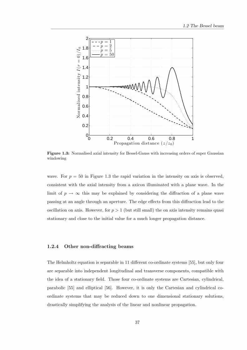
1.3 Normalised axial intensity for Bessel-Gauss with increasing orders of super
Gaussian windowing . . . . . . . . . . . . . . . . . . . . . . . . . . . . . . . 37
2.1 Plane wave vectors . . . . . . . . . . . . . . . . . . . . . . . . . . . . . . . . 46
2.2 Dispersion curves for Equation 2.35 (solid) and Equation 2.37 (dashed) for
I = 0 (black) and I > 0 (red) . . . . . . . . . . . . . . . . . . . . . . . . . . 48
3.1 Sample points for the FFT (o) and zeroth order QDHT (x). Separation of
QDHT points has been exaggerated for illustrative purposes. . . . . . . . . 63
3.2 Intensity comparison for axial point (r = 0) and first numerical point,
α1 = .3α2. . . . . . . . . . . . . . . . . . . . . . . . . . . . . . . . . . . . . . 65
3.3 Reconstruction error for test functions shown in Table 3.2. . . . . . . . . . . 68
3.4 Local relative error (δ) variation with step-length (solid), compared to
O(∆z3) estimate (dashed). . . . . . . . . . . . . . . . . . . . . . . . . . . . 72
3.5 Step error variation with (‘+’) and without (solid) adaptive step length . . 73
3.6 Step length (solid) and intensity on axis (dashed) . . . . . . . . . . . . . . 74
3.7 Guard band (red) and numerical band (black) for three successive grid sizes 76
3.9 Various bands for monitoring the aliased power . . . . . . . . . . . . . . . . 78
4.1 Euler diagram representing the sufficient conditions (white) and regions
which must be tested numerically (grey). . . . . . . . . . . . . . . . . . . . 89
4.2 Flow chart for numerically determining self-focusing behaviour. . . . . . . 91
21

LIST OF FIGURES
4.3 Comparison of the Townes profile, R0, to a Gaussian beam of equal power
and axial value. Radial co-ordinate, r, normalised to the Gaussian width, w0 92
4.4 Regions of global existence and collapse for the Townes profile. . . . . . . . 92
4.5 Regions of Global Existence (GE) and Collapse (CL) predicted by sufficient
conditions. Here Nc is the power of the Townes profile ||R0||22. Note that
there is no predicted variation with beam waist as expected. . . . . . . . . 93
4.6 Beam fate determined using HARP, sufficient condition for GE marked as
dashed line; cf Figure 4.5. . . . . . . . . . . . . . . . . . . . . . . . . . . . . 94
4.7 Comparison of collapse power for Gaussian and Bessel-Gauss beams . . . . 96
4.8 Regions of sufficient conditions for the Bessel-Gauss beam . . . . . . . . . 97
4.9 Collapse map for the Bessel-Gauss beam. Blue represents regions of Global
Existence, orange is blowup and green is collapse. . . . . . . . . . . . . . . 98
4.10 Higher resolution of area highlighted in Figure 4.9 . . . . . . . . . . . . . . 99
4.11 Maximum intensity for Bessel-Gauss beam for increasing power (w0 = 7.5),
positions in parameter space marked on Figure 4.9. . . . . . . . . . . . . . 100
4.12 Enlargement from Figure 4.9 showing propagation distance, normalised to
z0, before termination of the model. . . . . . . . . . . . . . . . . . . . . . . 101
5.1 Comparing results for Bessel-Gauss beams in linear and nonlinear media.
In both cases; k0r = 20, w0 = 5 and P = 2. . . . . . . . . . . . . . . . . . . . 106
5.2 Angular spectrum, obtained by numerically integrating Equation 5.8, k0rw0 =
100. . . . . . . . . . . . . . . . . . . . . . . . . . . . . . . . . . . . . . . . . 108
5.3 Transverse phase matching integral (Equation 5.17) for the Equation 5.16a 111
5.4 Transverse phase matching integral (Equation 5.18) for the second approx-
imation Equation 5.16b . . . . . . . . . . . . . . . . . . . . . . . . . . . . . 112
5.5 Figure 5.6d plotted on a log scale. . . . . . . . . . . . . . . . . . . . . . . . 114
5.6 Angular spectra for the numerically propagated Bessel-Gauss beam after
increasing propagation lengths. Initial Bessel-Gauss profile; P = 2, w0 = 5
and k0r = 20. Position of
√2k0
r is indicated as dotted line. . . . . . . . . . . 115
5.7 Frequency space diagram . . . . . . . . . . . . . . . . . . . . . . . . . . . . 115
5.8 Normalised axial intensity, w0 = 5, k0r = 20, P = 2. . . . . . . . . . . . . . 116
5.9 Modulation depth for Bessel-Gauss beam for increasing power. . . . . . . . 117
5.10 Spectrum at z = z0 for increasing power. . . . . . . . . . . . . . . . . . . . . 118
22

LIST OF FIGURES
5.11 Axial intensity for increasing power, w0 = 5, kr = 20. . . . . . . . . . . . . . 119
5.12 Beat length reducing with increasing power. . . . . . . . . . . . . . . . . . . 119
5.13 Frequency space diagram, increase in effective k indicated as ∆k. . . . . . . 120
5.14 Measured beat length (red ‘+’) and beat length equation (blue line) nor-
malised to the low power beat length (z0b ) . . . . . . . . . . . . . . . . . . . 121
5.15 Comparison of behaviour for Gaussian and super-Gaussian windows, w0 =
5, k0r = 20. . . . . . . . . . . . . . . . . . . . . . . . . . . . . . . . . . . . . 123
5.16 Normalised axial intensity for increasing powers, w0 = 5, k0r = 20, and
Gaussian window. . . . . . . . . . . . . . . . . . . . . . . . . . . . . . . . . 124
5.17 Normalised axial intensity for first beat period. Maximum marked as ‘x’,
notice the high frequency ripples present. . . . . . . . . . . . . . . . . . . . 125
5.18 Fast Fourier transform of intensity modulation . . . . . . . . . . . . . . . . 126
5.19 Scalogram of the axial intensity in Figure 5.16. . . . . . . . . . . . . . . . . 126
5.20 Scalogram for Gaussian and Super-Gaussian (m = 8) window. . . . . . . . . 128
5.21 Overlap region for Bessel-Gauss beam. . . . . . . . . . . . . . . . . . . . . 129
5.22 Axial intensity for a Bessel-Gauss beams propagating through full focus
(solid) and from the nominal focus (dashed) in a nonlinear medium w0 =
5,k0r = 20,P = 2. . . . . . . . . . . . . . . . . . . . . . . . . . . . . . . . . . 130
5.23 Axial intensity for a high-power Bessel-Gauss beam propagating through
full focus in a nonlinear medium, w0 = 5,k0r = 20,P = 3. . . . . . . . . . . . 131
5.24 Scalogram for full focus . . . . . . . . . . . . . . . . . . . . . . . . . . . . . 132
5.25 Improved equation for the chirped beat-length (Equation 5.31) α = 1.2. . . 133
5.26 Axial intensity for a seeded Bessel-Gauss beam propagating in the absence
of nonlinearity. . . . . . . . . . . . . . . . . . . . . . . . . . . . . . . . . . . 134
5.27 Axial intensity for varying u0g and φ. . . . . . . . . . . . . . . . . . . . . . . 137
5.28 Axial intensity for seeded beam for φ = 0 and φ = π. . . . . . . . . . . . . 138
5.29 Scalogram for seeded Bessel-Gauss beams. . . . . . . . . . . . . . . . . . . . 138
5.30 Bessel-Gauss beam propagating through full focus. Nominal focus of seed:
z = −0.5z0. Relative scaling used: u0g = 0.1u0
b , w1 = 3/k0r . . . . . . . . . . 139
5.31 Bessel-Gauss beam propagating through full focus. Nominal focus of seed:
z = 0. Relative scaling used: u0g = 0.05u0
b , w1 = 3/k0r . . . . . . . . . . . . . 139
23

LIST OF FIGURES
5.32 Axial intensity for nonparaxial Bessel-Gauss beam; θ = 35, k0r = 20, w0 = 5,
P = 4 (1.5Pc). . . . . . . . . . . . . . . . . . . . . . . . . . . . . . . . . . . 141
5.33 Axial intensity for nonparaxial Bessel-Gauss beams for increasing inner cone
angles; k0r = 20, w0 = 5, P = 2. . . . . . . . . . . . . . . . . . . . . . . . . 142
5.34 Measured nonparaxial beat length θ = 30◦. . . . . . . . . . . . . . . . . . . 143
5.35 Normalised axial intensity for a Bessel-Gauss beam, w0 = 5, k0r = 20 and
P = 2.5 . . . . . . . . . . . . . . . . . . . . . . . . . . . . . . . . . . . . . . 143
6.1 Solutions to Equation 6.2. Note: B(0) = 1 in both cases. . . . . . . . . . . . 148
6.2 Solutions to Equation 6.5 . . . . . . . . . . . . . . . . . . . . . . . . . . . . 150
6.3 Radial profile of nonlinear Bessel functions along with a linear Bessel func-
tion for comparison . . . . . . . . . . . . . . . . . . . . . . . . . . . . . . . 150
6.4 Comparison of linear and nonlinear Bessel beams of equal power in the
central lobe. . . . . . . . . . . . . . . . . . . . . . . . . . . . . . . . . . . . 152
6.5 Comparison of linear and nonlinear Bessel beams for matched frequency in
outer lobes. . . . . . . . . . . . . . . . . . . . . . . . . . . . . . . . . . . . 153
6.6 Intensity profile for propagation in a Nonlinear medium . . . . . . . . . . 156
6.7 Intensity profile for propagation in a Linear medium . . . . . . . . . . . . 157
6.9 Axial intensity for linear and nonlinear Bessel beams with a super Gaussian
envelope, p = 4. . . . . . . . . . . . . . . . . . . . . . . . . . . . . . . . . . 159
6.10 Comparison of axial intensity for nonparaxial linear and nonparaxial non-
linear Bessel beams . . . . . . . . . . . . . . . . . . . . . . . . . . . . . . . 161
6.11 Radial profiles for higher-order nonlinear Bessel beams, n = 1 . . . . . . . 164
6.12 Intensity profiles in a nonlinear medium. . . . . . . . . . . . . . . . . . . . 165
24

List of Tables
3.1 Speed and relative accuracy for symmetrised split-step methods . . . . . . . 62
3.2 Typical beam-like functions. . . . . . . . . . . . . . . . . . . . . . . . . . . . 69
3.3 Accuracy of field on axis and relative speed for each method. . . . . . . . . 70
3.4 Decision process for adaptive step length. . . . . . . . . . . . . . . . . . . . 73
3.5 Speed and global accuracy for adaptive step length . . . . . . . . . . . . . . 75
3.6 Comparison of speeds for adaptive techniques when propagating a Gaussian
beam below the critical power. . . . . . . . . . . . . . . . . . . . . . . . . . 80
3.7 Comparison of speeds for adaptive techniques when propagating a Bessel-
Gauss beam. . . . . . . . . . . . . . . . . . . . . . . . . . . . . . . . . . . . 81
4.1 Decision table for sufficient conditions . . . . . . . . . . . . . . . . . . . . . 88
4.2 Critical power for blowup of the Gaussian beam . . . . . . . . . . . . . . . . 95
6.1 Stationary solutions . . . . . . . . . . . . . . . . . . . . . . . . . . . . . . . 149
6.2 Full beam power, w0 = 30WFWHM . . . . . . . . . . . . . . . . . . . . . . . . 154
B.1 Time take to execute FFT . . . . . . . . . . . . . . . . . . . . . . . . . . . 186
25

LIST OF TABLES
26

Chapter 1
Introduction
Recently much interest has surrounded the potential for waveguide fabrication in highly
nonlinear materials such as Heavy Metal Oxide (HMO) glass using ultra-fast pulsed laser
systems [1, 2, 3, 4]. Such materials have the potential to provide an excellent basis for
nonlinear optical integrated devices such as optical switches and frequency converters [5].
However, this high nonlinearity also presents a problem. As Siegel et al. discovered [1],
the high nonlinear refractive index can cause the beam used to fabricate the waveguide to
self focus before the threshold for optical breakdown is achieved; clearly another approach
is required.
This thesis addresses the behaviour of Bessel and Bessel-like beams in Kerr-like nonlin-
ear materials with a view to applying this to the fabrication of integrated optical compo-
nents in materials with a high nonlinear refractive index. This begins with a brief history
of integrated optics, outlining why fabrication by direct laser writing is important, ad a
review of some of the basic properties of Bessel beams in linear media.
1.1 Integrated optical structures
The term “integrated optics” was first used by S. E. Miller [6] while working at Bell
Labs. In his seminal paper, he describes the similarity of integrated optics by analogy
to the recently developed integrated circuits (IC). In an integrated-circuit, electrons are
manipulated by components such as transistors, forming the basis of a control structure.
Miller proposed devices designed to act as circuits for photons embedded, just like ICs,
on a single planar substrate. Many common optical components can be integrated; these
27

Chapter 1: Introduction
include beam splitters, gratings, polarisers, interferometers [7] and nonlinear devices [8]. A
good overview of typical devices and their application can be found in texts by Hunsperger
and Lifante [9, 10]. Although these devices were first proposed in the late 60s it took several
years before the techniques were available to combine them properly into the integrated
optical circuits proposed by Miller.
1.1.1 Device Fabrication
A common substrate for device integration is lithium niobate (LiNbO3), which exhibits
electro-optic, acousto-optic, nonlinear, and birefringent behaviour. The wide range of
behaviour exhibited by LiNbO3 allows the construction of switches, modulators, cou-
plers, wavelength division multiplexers (WDM), and dense wavelength division multiplex-
ers (DWDM)[11]. Other substrates used include multi glass compounds, SiOxNy:SiO2:Si
and TiO2:SiO2:Si, III-V compounds (InP, GaAs) and polymers [10].
A common technique for integrating optical devices is photolithography; here a mask
is placed on a photosensitive material covering the substrate. A laser, or other uniform
light source, is then used to expose the area of the photosensetive material not protected
by the mask. Typically the mask material will become more soluble after exposure. A
solvent is then used to remove unwanted photoresist. Once the surface of the substrate has
been exposed waveguiding structures may be fabricated in a number of ways , including
out diffusion, in diffusion and proton exchange [12].
One problem with these techniques is the lack of control over the refractive index
of the device. To create high quality single mode waveguides a high degree of accuracy
is required when varying the refractive index. In devices where the refractive index is
required to vary with position the techniques described above must be applied iteratively,
which is time consuming and not always that effective.
1.1.2 Direct Laser Writing
First demonstrated by Hirao et al. [13] in 1996, direct laser writing uses a laser to perma-
nently modify the refractive index of a material allowing the construction of waveguides
and subsequently many other elements. Direct laser writing has the advantage of being
mask-less therefore removing several steps from the process. Ultimately this makes it
cheaper and less labour intensive to make successive prototypes. This is in comparison to
28
1.1 Integrated optical structures
the photolithography methods mentioned above for which a separate mask must be made
for each prototype. Another benefit of direct laser writing is the ability to spatially vary
the longitudinal refractive index of the area being written, a process that is extremely
difficult with a photolithographic mask. Furthermore the process can be applied to selec-
tive areas of the device, so that each element can be written independently. Direct laser
writing has been performed in a variety of materials including GaAs, LiNbO3, fused silica,
and polymers [14, 15].
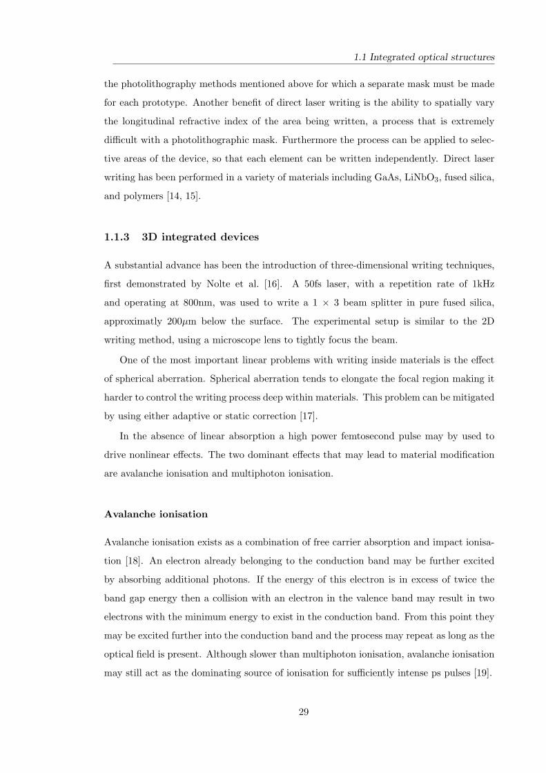
1.1.3 3D integrated devices
A substantial advance has been the introduction of three-dimensional writing techniques,
first demonstrated by Nolte et al. [16]. A 50fs laser, with a repetition rate of 1kHz
and operating at 800nm, was used to write a 1 × 3 beam splitter in pure fused silica,
approximatly 200µm below the surface. The experimental setup is similar to the 2D
writing method, using a microscope lens to tightly focus the beam.
One of the most important linear problems with writing inside materials is the effect
of spherical aberration. Spherical aberration tends to elongate the focal region making it
harder to control the writing process deep within materials. This problem can be mitigated
by using either adaptive or static correction [17].
In the absence of linear absorption a high power femtosecond pulse may by used to
drive nonlinear effects. The two dominant effects that may lead to material modification
are avalanche ionisation and multiphoton ionisation.
Avalanche ionisation
Avalanche ionisation exists as a combination of free carrier absorption and impact ionisa-
tion [18]. An electron already belonging to the conduction band may be further excited
by absorbing additional photons. If the energy of this electron is in excess of twice the
band gap energy then a collision with an electron in the valence band may result in two
electrons with the minimum energy to exist in the conduction band. From this point they
may be excited further into the conduction band and the process may repeat as long as the
optical field is present. Although slower than multiphoton ionisation, avalanche ionisation
may still act as the dominating source of ionisation for sufficiently intense ps pulses [19].
29

Chapter 1: Introduction
Multiphoton ionisation
An atom may be ionised by absorbing multiple photons at the same time given
nhν ≥ Eg, (1.1)
where n is the number of photons absorbed, hν is the photon energy, and Eg is the
bandgap energy. This form of ionisation leads to strong plasma formation and permanent
local material modification [20]; however this occurs on a much shorter timescale compared
to avalanche ionisation and as a result non-local material modification from thermal stress
is avoided. The behaviour of multiphoton ionisation is threshold-like in intensity, for silica
glass the threshold is around 1011 W/cm2.
Using a fs pulsed laser system, multiphoton ionisation may be exploited to deposit en-
ergy before thermal diffusion increases the affected area. Furthermore a larger wavelength
may be used resulting in a photon energy below the bandgap energy. This prevents single
photon absorption into the material prior to the focus resulting in more accurate writing
and better quality waveguides [21].
Many devices have been sucessfuly fabricated using femtosecond direct laser writing,
including relief gratings [22], fiber Bragg gratings [23], channel waveguides and Y-couplers
[15], and active waveguides [24].
1.1.4 Heavy metal oxide glass
Heavy metal oxide (HMO) glasses can be defined as glass containing over 50 cat.% Bi
or Pb [25]. The low phonon energy [26] means they have excellent transmission into the
far IR with λ < 6-7µm. One of the problems encountered when attempting to write to
this material is the relatively high nonlinear refractive index [27] (n2 = 10−18 − 10−19
m2/Wcompared to n2 = 10−20 m2/W for silica), using conventional fs writing techniques
this may cause the beam to self-focus within the material before the threshold for multi-
photon ionisation is exceeded. This self-focusing may lead to filament formation as was
observed by Siegel et al. [1]. Although this may result in structures capable of waveguid-
ing, it was noted by Zoubir et al. [28] that this is due to the non-local thermal stress in
the material as the waveguiding occurs away from the region directly modified through
avalanche ionisation.
30

1.1 Integrated optical structures
Another approach to waveguide writing in HMO glass is to use an astigmatic beam
formed from a slit [3]; such techniques have been successfully applied to write waveguides
in HMO glasses [3, 29]. However, a distinctive ‘bite mark’ is clearly visible which may be
attributed to the self-focusing of the beam.
It is likely that in addition to Kerr nonlinearity other nonlinear effects will occur when
attempting to write structures. However, in HMO glasses the predominant beam reshaping
effect is attributable to Kerr self-focusing [30]. Nonlinear absorption may also occur;
however, this is neglected for the purposes of this thesis in order improve understanding
of the behaviour of Bessel beams in Kerr-like nonlinear materials.
1.1.5 Writing techniques
Several techniques have been developed for writing structures in optical materials. These
techniques vary from the highly versatile, but time consuming, technique of point-by-point
raster scanning to extremely rapid but inflexible techniques such as volume holography
[31]. Some techniques exist as a compromise between versatility and speed such the use
of cylindrical lenses to create optical volume gratings [32].
Rather than attempting to avoid the effects of self-focusing when writing structures
in highly nonlinear materials such as HMO glass, this thesis proposes that the behaviour
may be harnessed for certain beam profiles such as the Bessel beam (Chapter 5). This
turns a problem into an advantage. The on-axis intensity of a Bessel-Gauss beam in a
nonlinear medium is known to be periodically modulated in the direction of propagation
[33, 34, 35, 36]. If harnessed, this periodic modulation may lead to a versatile and rapid
technique. If fine control is available over the period and intensity of modulation then,
combined with raster scanning, this technique may be applied to generate volume photonic
structures with a high degree of control over the spacing and separation.
It has already been demonstrated that the Bessel-Gauss beam may be used to generate
high aspect ratio micro channels, with the absence of substantial nonlinear effects, within
glass samples [37]. Furthermore Bessel-Gauss beams have been successfully employed to
fabricate periodic structures in the presence of nonlinear absorption for powers well in
excess of the critical self-focusing threshold [38].
However, much is still not understood about the behaviour of the Bessel-Gauss beam
in Kerr-like nonlinear materials. Therefore, in order to assess the feasibility of periodic
31

Chapter 1: Introduction
structure formation using the Bessel-Gauss beam it is necessary to first study the behaviour
of such beams and their evolution in Kerr-like nonlinear materials.
For the purpose of this study the effect of nonlinear absorption has been neglected. This
mechanism has already been studied for the generation of periodic structures using Bessel
beams [37]. This thesis aims to investigate the propagation of Bessel-Gauss beams within a
material exhibiting Kerr like nonlinearity. In the absence of linear or nonlinear absorption
the mechanism for material modification relies on the maximum intensity exceeding the
optical breakdown threshold within the material.
1.2 The Bessel beam
First introduced by Durnin, [39, 40], the Bessel beam represents a, so called, diffraction
free solution to the Helmholtz wave equation
E(r, z) = exp(ikzz)J0
(k0
rr), (1.2)
where J0 is the zero-Bessel function of the first kind and the principal transverse spatial
frequency, k0r , and longitudinal spatial frequency kz are related to the wave number in the
material, k0, by (k0r)
2 + k2z = k2
0. Only the phase of such beams varies in the direction
of propagation (z), and consequently there is no variation in the intensity profile as the
beam evolves
I(r, z > 0) = I(r). (1.3)
However, because the intensity of such a beam decays as r−1 the total power is tech-
nically unbounded. The Bessel beam does not constitute a, physically realisable, beam
profile. If the Bessel beam is truncated then, like a plane wave, it is no longer a separable
solution to the wave equation and is therefore no longer diffraction free.
A typical approximation for theoretical and analytical studies it to apply a Gaussian
envelope to the Bessel profile, thus ensuring the beam is of finite power [41, 42, 43, 44].
32

1.2 The Bessel beam
1.2.1 Derivation
The Bessel beam may be derived from the Helmholtz wave equation
(∇2 − k2
)E(r, z, t) = 0, (1.4)
by separating the solution in to a transverse profile and longitudinal phase
E(r, t) = exp(−ikzz)A(r). (1.5)
If a cylindrically symmetric co-ordinate system is adopted, substituting Equation 1.5 into
Equation 1.4 yields the ODE
(∂2
∂r2+
1r
∂
∂r+
ω2
c2− k2
z
)A(r) = 0, (1.6)
which is equivalent to Bessel’s equation [45]. A solution to Equation 1.6 is therefore given
by the zero-order Bessel function of the first kind,
A(r) = A0J0(k0rr), (1.7)
where k0r =
√k2 − k2
z and k = ω/c.
It should be noted that the Fourier transform of the Bessel function is given by a ring
in frequency space;
F{J0(k0
rr)}
(kr) = δ(kr − k0r). (1.8)
As a consequence of this, the Bessel beam may be considered as the interference pattern
from a conical set of plane waves. The angle made between this cone and the optical axis
shall be referred to as the inner cone angle, θ, and may be defined as
θ = tan−1
(k0
r
kz
). (1.9)
1.2.2 Physical generation
Several methods have been developed for physically generating Bessel-like beams. These
include formation from a circular annulus [39], focusing from an axicon lens [46, 47] and
33

Chapter 1: Introduction
formation from a hologram [48, 49]. Other methods have successfully been employed such
as the use of a Fabry-Perot cavity in addition to a circular annulus [47]. Additionally
laser cavities have been developed using axicon elements and conical mirrors to produce
a Bessel-Gauss output [50, 51].
Circular annulus
Owing to the fact that the Fourier transform of the Bessel function is essentially a ring in
frequency space, Durnin initially proposed that the Bessel-beam may be created by evenly
illuminating an annular aperture in the back focal region of a lens. The focused light from
the lens will produce a quasi Bessel profile at the focal point of the lens. The inner cone
Figure 1.1: Formation of a Bessel beam from an annulus
angle of a Bessel beam created in this manner may be expressed as
θ = tan−1
(d
2f
), (1.10)
where d is the diameter of the annulus and f is the focal length of the lens [39]. The geo-
metric shadow length is the term given to the characteristic propagation length exhibited
by the Bessel beam. From Figure 1.1 it is clear that this length is the length over which
the axial position is illuminated by the cone of plane waves formed from the annulus. The
geometric shadow length, z0, may be written as
z0 =R
tan θ, (1.11)
34

1.2 The Bessel beam
where R is the radius of the imaging lens.
It was observed by Durnin et al. [39] that the intensity close to the optical axis varied
rapidly in the direction of propagation before dropping off suddenly at z0. Additionally if
the annulus is illuminated by a Gaussian beam a considerable amount of power is blocked
by the annulus. As a result this method is primarily of conceptual interest and is generally
not used to produce Bessel beams.
Axicon lens
Another method for creating a Bessel beam is to use an axicon, or conical, lens. The
principle behind this setup is shown in Figure 1.2. From Figure 1.2 it becomes clear that
Figure 1.2: Bessel beam formation with an axicon lens
the Bessel beam is formed from a cone of plane waves. and may be determined from the
properties of the axicon by
θ = α(n0 − 1), (1.12)
where n0 is the refractive index of the lens material and α is the internal angle of the
axicon lens marked on Figure 1.2. For small angles, θ, the geometric shadow length, z0
may be written [42] as
z0 = kw0
k0r
, (1.13)
where w0 is the width of the Gaussian beam.
35

Chapter 1: Introduction
If the axicon is illuminated with a plane wave then a similar oscillation of intensity
close to the optical axis is observed [42], however if a Gaussian beam is used instead
then a much smoother variation in intensity is observed close to the optical axis. A good
numerical approximation to this is the Bessel-Gauss beam (Section 1.2.3).
Hologram
Holographic techniques may be used to form Bessel-like beams by applying the phase
appropriate to a Bessel beam onto an input Gaussian beam. These holograms were ini-
tially etched permanently onto a material surface [52], however more recently computer
controlled Spatial Light Modulators (SLM) have been used [49, 53].
Using an SLM is by far the most versatile method for generating Bessel-like beams
as it allows the profile to be varied rapidly, potentially allowing the profile to be varied
across one pulse by acting in the spatio-temporal Fourier domain. Additionally the profile
is not restricted to a Bessel-Gauss profile and it has been demonstrated that an SLM
may be used to tune the intensity on axis for Bessel-like beams [48]. One of the major
disadvantages for using an SLM is the poor efficiency; typically only 40% of the input
power is present in the first diffraction order [54].
1.2.3 Numerical description
A reasonable approximation to the Bessel beam that is representative of the beams created
with both axicon lenses and holographic techniques is the Bessel-Gauss beam. Here a
Gaussian or super-Gaussian window is used to ensure finite power,
E(r, z = 0) = E0J0(k0rr) exp
[−(
r
w0
)2p]
, (1.14)
where w0 is the width of the Gaussian window and pth order of the super-Gaussian window.
In the case of small inner cone angles, the geometric shadow length, z0 may be calculated
from Equation 1.13.
The normalised intensity on axis is plotted in Figure 1.3 for a Bessel-Gauss beam
propagating in a linear medium. For the Gaussian window (p = 1) the intensity decays
smoothly, as expected, but as p → ∞ the super Gaussian tends to a top hat profile of
radius w0 which is good description of an axicon lens illuminated by an incident plane
36
1.2 The Bessel beam
0 0.2 0.4 0.6 0.8 10
0.2
0.4
0.6
0.8
1
1.2
1.4
1.6
1.8
2
Propagation distance (z/z0)
Norm
ali
sed
inte
nsi
tyI(r
=0)/
I0
p = 1p = 2p = 5p = 50
Figure 1.3: Normalised axial intensity for Bessel-Gauss with increasing orders of super Gaussianwindowing
wave. For p = 50 in Figure 1.3 the rapid variation in the intensity on axis is observed,
consistent with the axial intensity from a axicon illuminated with a plane wave. In the
limit of p → ∞ this may be explained by considering the diffraction of a plane wave
passing at an angle through an aperture. The edge effects from this diffraction lead to the
oscillation on axis. However, for p > 1 (but still small) the on axis intensity remains quasi
stationary and close to the initial value for a much longer propagation distance.
1.2.4 Other non-diffracting beams
The Helmholtz equation is separable in 11 different co-ordinate systems [55], but only four
are separable into independent longitudinal and transverse components, compatible with
the idea of a stationary field. Those four co-ordinate systems are Cartesian, cylindrical,
parabolic [55] and elliptical [56]. However, it is only the Cartesian and cylindrical co-
ordinate systems that may be reduced down to one dimensional stationary solutions,
drastically simplifying the analysis of the linear and nonlinear propagation.
37

Chapter 1: Introduction
1.3 Thesis Overview
This thesis presents a study of the behaviour of Bessel-like beams evolving in Kerr-like
nonlinear materials. Although this work is motivated by the desire to allow the construc-
tion of periodic structures in highly nonlinear HMO glasses much of the following work is
of more general interest.
1.3.1 Chapter 2
In order to understand the effect nonlinearity has on the construction of integrated optical
components by direct laser writing, it is first necessary to understand the behaviour of
optical beams in the presence of self-focusing nonlinearity.
Starting from Maxwell’s equations a nonlinear wave equation is derived that shall form
the basis for most of the work in this thesis on the nonlinear evolution of optical beams. In
order to evaluate this nonlinear wave equation, a numerical model is required. The merits
and deficiencies of various finite difference methods are discussed and it is concluded that
these should be discarded where possible in favour of pseudo spectral split step method
for nonlinear paraxial propagation.
For quasi-nonparaxial beams it is noted that the pseudo spectral split-step methods
are considerably less accurate. As a solution to this, a hybrid pseudo spectral technique
is discussed; the longitudinal derivative is evaluated using a finite difference method and
the transverse derivatives are evaluated using the highly efficient fast Fourier transform.
1.3.2 Chapter 3
Numerical evolution of nonlinear optical problems can be a time consuming process; there-
fore it is desirable to use a highly efficient numerical method wherever possible. Since the
Bessel beam is radially symmetric, it is possible to adapt the split-step method introduced
in the previous chapter for one dimensional, radially symmetric, propagation. Although
this means that the less efficient Quasi-Discrete Hankel Transform (QDHT) must be used
– compared to the fast Fourier transform – the reduction to one dimension ultimately
results in a considerably faster model.
One problem incurred by using the QHDT is the uneven spacing of the sample points
associated with this transform and in particular the absence of a point on axis for some
38

1.3 Thesis Overview
beams. This is addressed, for the first time, by applying the generalised sampling formula
to derive a reconstruction formula.
In order to maximise efficiency, adaptive techniques are applied to the model in both
the step length and transverse grid size. The step length is dynamically modified based
on a local error technique developed for Cartesian co-ordinates by Sinkin et al. [57]. In
the transverse dimension a dynamic technique is implemented by which the beam size in
both real and frequency space is monitored and the grid size adjusted accordingly. It is
demonstrated how the inclusion of the various adaptive techniques affects the efficiency
and accuracy of the numerical model.
1.3.3 Chapter 4
One situation where an adaptive model is particularly important is for beams close to or
above the threshold power for critical self-focusing. Often the terms blowup and collapse
are used interchangeably to describe critical self-focusing. This chapter introduces a more
mathematical approach to the definitions of self-focusing, categorising the beam fate into
either global existence, blowup or collapse and clarifies their meaning unambiguously and
in an accessible fashion.
By reproducing previously observed boundaries for Gaussian critical self-focusing, it
is demonstrated that HARP is a suitable tool for determining the beam fate for radially
symmetric beams. The sufficient conditions for the Bessel-Gauss beam fate are shown to
be semi-analytic and when evaluated it is clear that a much larger region of parameter
space must be investigated numerically. When probed numerically, it appears that for cer-
tain regions of parameter space increasing the power of Bessel-Gauss beams may actually
prevent critical self-focusing!
1.3.4 Chapter 5
In the sub-critical region, the Bessel-Gauss beam is known to exhibit a periodic intensity
modulation in the direction of propagation. This modulation affects the whole beam,
however it is the modulation of the axial lobe that is of particular interest in the context
of integrated optics. If it is possible to accurately control the period of modulation then it
may be possible to use this behaviour to write structures in materials with a high nonlinear
refractive index such as HMO glasses.
39

Chapter 1: Introduction
The origins of this periodic intensity modulation are discussed and it is noted that
the existing equations describing the length of this modulation become inaccurate as the
power is increased. A correction is proposed based on a modification to the existing beat
length equation and the accuracy of this correction is discussed in both the paraxial and
quasi-nonparaxial regime. It is noted that the period of modulation is not constant along
the beam and that a negative chirp in frequency is observed as the beam evolves. This
modification in modulation length is investigated in the context of the modified, power-
dependent, beat length equation.
Additionally the possibility of using a ‘seed’ beam is investigated. A seed beam would
be a low power Gaussian super-imposed on the central lobe of the Bessel-Gauss beam.
Adjusting the phase of this seed relative to the Bessel-Gauss beam allows the position of
the maxima to be varied with great precision.
1.3.5 Chapter 6
This chapter builds on the work of Johannisson et al. [34] by considering stationary so-
lutions to the nonlinear wave equation as an analogy to the linear wave equation. It is
noted that in addition to the well studied Townes profile, there exists a set of stationary
solutions to the nonlinear wave equation for positive eigenvalues. Due to the similarity
with the Bessel function, J0 these functions are given the name nonlinear Bessel functions.
The profile and axial intensity evolution of linear and nonlinear Bessel beams – in a
nonlinear medium – are compared. It is shown that the nonlinear Bessel beams exhibit
the anticipated quasi-stationary behaviour. The existence of nonlinear Bessel beams is
investigated for initial profiles possessing azimuthal phase and a set of boundary condi-
tions are derived for integer order nonlinear Bessel beams. These higher-order nonlinear
Bessel beams are shown to also exhibit quasi-stationary behaviour as they propagate in a
nonlinear medium.
40

Chapter 2
Understanding self-focusing
To understand the behaviour of Bessel beams in a material with a high nonlinear refractive
index it is first helpful to understand the process behind the nonlinearity. This chapter
deals with the derivation of the nonlinear refractive index and the construction of nonlinear
wave equations.
These nonlinear wave equations are then discretised, in order to produce a scheme
to numerically evaluate the propagation of an initial field through a Kerr-like medium.
Both finite difference and pseudo spectral methods are considered in the paraxial and
quasi-nonparaxial limit and it is established that pseudo spectral methods are preferable
in terms of stability, accuracy and efficiency.
2.1 The nonlinear refractive index
Within a classical framework and under low intensities of incident light, the polarisation
of a material, P, varies harmonically in proportion to the field strength. As the intensity
is increased this assumption breaks down and the full polarisation vector must taken into
account
P = ε0
(χ(0) + χ(1)(E) + χ(2)(E,E) + χ(3)(E,E,E) + ...
), (2.1)
where χ(k) is the kth order susceptibility – generally a tensor of rank k + 1. The second-
order term, χ(2), is responsible for the DC Pockels effect and second harmonic generation
and, along with the other even-order terms, is generally ignored for most silica based
materials due to the molecular symmetry [58]. Provided the optical field is still small
compared to the Coulomb binding field, the higher-order terms contribute significantly
41

Chapter 2: Understanding self-focusing
less than the lower-order terms and the polarisation may be truncated at χ(3). If the light
is assumed to be linearly polarised in x and nonlinear birefringence can be ignored the
material polarisation may be written as
Px = ε0χ(1)xx Ex + ε0χ
(3)xxxxE3
x. (2.2)
If the polarised electric field, Ex, and material polarisation, Px are written in the
time-harmonic form
Ex = x12
(E exp(−iωt) + E∗ exp(iωt)) , (2.3)
Px = x12
(P exp(−iωt) + P ∗ exp(iωt)) , (2.4)
then Equation 2.2 may be written as
P = ε0χ(1)xx E + ε0χ
(3)xxxx|E|2E, (2.5)
where the terms for third harmonic generation have been discarded. It is convenient to
separate the polarisation into the linear, PL, and nonlinear, PNL, parts such that
P = PL + PNL, (2.6)
where
PL = ε0χ(1)xx E, PNL = ε0χ
(3)xxxx|E|2E. (2.7)
The total polarisation may be written using an effective susceptibility, χeff as
P = ε0χeffE, (2.8)
which may also be separated into the linear and nonlinear components
χL = ε0χ(1)xx , χNL = ε0χ
(3)xxxx|E|2. (2.9)
42

2.2 Critical self-focusing
By analogy with the linear case, the refractive index may be written as
n =√
1 + χeff . (2.10)
Using the binomial expansion this may be approximated as
n = n0
(1 +
12n2
0
χNL
), (2.11)
where n0 is the linear refractive index, defined as n0 =√
1 + χL . This may be written as
n =n0 +38χ(3)
xxxx|Ex|2, (2.12)
=n0 + n2I, (2.13)
where I = |E|2 and n2 = 38χ
(3)xxxx.
This result is the well-known intensity-dependent refractive index due to the optical
Kerr effect [58].
It should be noted that the above derivation is concerned solely with the construction
of a nonlinear refractive index. In practice other nonlinear processes may also be present,
such as second- and third-harmonic generation and stimulated Raman scattering.
2.2 Critical self-focusing
Probably, the most well known example of Kerr-like nonlinearity is the case of critical
self-focusing. This is a process by which the intensity-dependent refractive index change
causes a lens like profile to be formed within the material. For sufficiently powerful beams
this may cause the beam to collapse to a point within the material. Physically this will
manifest itself in the intensity exceeding the threshold for permanent material modification
and could lead to a damaged region.
For a simple Gaussian beam
E(r, z = 0) = E0 exp(−r2), (2.14)
43

Chapter 2: Understanding self-focusing
the instantaneous refractive index change, from Equation 2.13, may be written as
n(r) = n0 + n2|E0|2 exp(−2r2). (2.15)
Taylor expanding this around r = 0 yields
n(r) = n0 + |E0|2n2 − 2|E0|2n2r2, (2.16)
where the last term may be immediately identified as a simple thin lens. This lensing term
causes the beam to ‘self-focus’
If the self-focusing is not outweighed by the linear diffraction then the beam will come
to a focus within the material. By finding the point at which the self-focusing exactly
balances the diffraction a critical power threshold, Pc, may be determined, above which
the beam will undergo critical self-focusing [59, 60]
Pc 'λ2
8πn0n2. (2.17)
The accuracy of Equation 2.17 for beams other than the Gaussian is addressed more
rigorously in Chapter 4.
2.3 A nonlinear wave equation
Modelling the propagation of an optical field using the full Maxwell equations would prove
too costly in terms of computational time. Instead Maxwell’s equations are reduced down
to the nonlinear wave equation.
Maxwell’s equations in SI units may be written as
∇×E = −∂B∂t
, (2.18a)
∇×H = J +∂D∂t
, , (2.18b)
∇.D = ρf , (2.18c)
∇.B = 0. (2.18d)
In the absence of currents and free charges, J = 0 and ρf = 0.
44

2.3 A nonlinear wave equation
In non-magnetic media, the flux densities, D and B are related to the electric and
magnetic fields by constitutive relations
D = ε0E + P, (2.19)
B = µ0H, (2.20)
where ε0 and µ0 are the vacuum permittivity and magnetic permeability respectively and P
is the induced electric polarisation. By taking the curl of Equation 2.18a and substituting
in Equation 2.20 the following equation may be written
∇×∇×E = −µ0∂
∂t(∇×H) . (2.21)
Applying the relation in Equation 2.18b and then Equation 2.19 yields
∇×∇×E = − 1c2
∂2E∂t2
− µ0∂2P∂t2
. (2.22)
If the electric field is assumed to be polarised in the x direction and the field and induced
polarisation are assumed to have the time-harmonic form from Equation 2.3 then this may
be written as
∇×∇×E =ω2
c2
((1 + χ(1)
xx )E + χ(3)xxxx|E|2E
). (2.23)
This may be re-written using the linear and nonlinear refractive indices such that
∇×∇×E =ω2
c2
(n2
0E + n2|E|2E). (2.24)
By using the identity
∇×∇×E = ∇(∇.E)−∇2E = −∇E2, (2.25)
Equation 2.24 may be written as a nonlinear wave equation. In particular this is known
as the nonlinear Helmholtz equation owing to it similarity to the linear equation [61],
∂2E
∂z2+∇2
⊥E + k2E + 2k2n2/n0|E|2E = 0, (2.26)
45

Chapter 2: Understanding self-focusing
where ∇2⊥ is the transverse Laplace operator and, in Cartesian co-ordinates, is given by
∇2⊥ =
∂2
∂x2+
∂2
∂y2. (2.27)
This nonlinear Helmholtz equation shall serve as the starting point for all of the numerical
models discussed and implemented in this thesis.
2.3.1 The nonlinear Schrodinger equation
To simplify the numerical modelling of this equation a normalisation is taken, consistent
with a predominantly forward propagating wavefront
E(x, y, z) = u(x, y, z) exp(ikz). (2.28)
A plane wave, E, with wave vector k1 = (kx, ky, kz), propagating predominantly in
the forward direction, is shown in Figure 2.1a. When Equation 2.28 is applied the wave
vector for u may expressed as
k1 = k1 − k, (2.29)
where k = (0, 0, k). The net effect of this means that the z component of the wave vector,
kz, is much smaller than that of the original wave vector, kz, for paraxial waves. This is
beneficial for the modelling of paraxial systems because the rate of change of the field will
be smaller and consequently larger steps may be taken.
(a) Forward propagating (b) Backward propagating
Figure 2.1: Plane wave vectors
It should be noted that this step does not explicitly preclude the existence of counter
propagating fields. An example of a counter propagating plane wave is shown in Figure
46
2.3 A nonlinear wave equation
2.1b. In this case the modified wave vector has a much larger z component and a counter
propagating plane wave evolves as u(z) = exp(−i2kzz).
If the z derivative in Equation 2.26 is expanded using Equation 2.28 the Nonparaxial
Nonlinear Schrodinger Equation (NNSE) is obtained [62]
∂2u
∂z2+ 2ik
∂u
∂z+∇2
⊥u + 2k2n2/n0|u|2u = 0, (2.30)
from which the exp(−ikz) term has been factored out.
Typically it is convenient to normalise Equation 2.30 with respect to a reference, linear,
Gaussian beam of the form
u(x) = exp
[−(
x
w0
)2]
, (2.31)
such that x = x/w0, z = z/Ld where Ld is the diffraction length, Ld = kw20/2, and the
field is scaled as u(x, z) =√
kn2/n0Ld u(x, z). This results in a scaled nonlinear wave
equation
κ∂2u
∂z2+ i
∂u
∂z+∇2
⊥u + |u|2u = 0, (2.32)
where the constant κ = (kw0)−1 is a measure of the nonparaxiality of the beam.
By considering a plane wave solution [63]
u(x, y, z) = u0 exp[i(kxx + kyy + kz z)
], (2.33)
a dispersion relation may be written for the NNSE as
κk2z + kz +
12k2
x +12k2
y − |u0|2 = 0. (2.34)
This may then be solved for the longitudinal wave number, kz
kz = − 12κ± 1
2κ
√1− 4κ
(12(k2
x + k2y)− |u0|2
). (2.35)
If the field is slowly varying in z then the Slowly Varying Envelope Approximation
(SVEA) may be taken and the second derivative in z discarded from Equation 2.32, leaving
i∂u
∂z+∇2
⊥u + |u|2u = 0. (2.36)
47
Chapter 2: Understanding self-focusing
Equation 2.36 is referred to as the Nonlinear Schrodinger Equation (NSE) – with a power
nonlinearity (Section 4.1). This equation forms the basis for much of the work on paraxial
nonlinear optics. Again, by considering plane wave propagation, a dispersion relation for
Equation 2.36 may be written as,
kz = −12k2
x −12k2
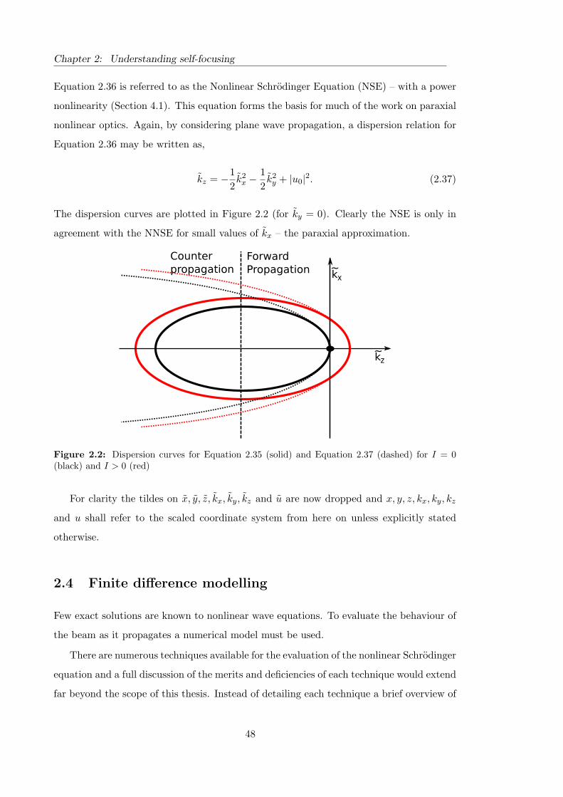
y + |u0|2. (2.37)
The dispersion curves are plotted in Figure 2.2 (for ky = 0). Clearly the NSE is only in
agreement with the NNSE for small values of kx – the paraxial approximation.
Figure 2.2: Dispersion curves for Equation 2.35 (solid) and Equation 2.37 (dashed) for I = 0(black) and I > 0 (red)
For clarity the tildes on x, y, z, kx, ky, kz and u are now dropped and x, y, z, kx, ky, kz
and u shall refer to the scaled coordinate system from here on unless explicitly stated
otherwise.
2.4 Finite difference modelling
Few exact solutions are known to nonlinear wave equations. To evaluate the behaviour of
the beam as it propagates a numerical model must be used.
There are numerous techniques available for the evaluation of the nonlinear Schrodinger
equation and a full discussion of the merits and deficiencies of each technique would extend
far beyond the scope of this thesis. Instead of detailing each technique a brief overview of
48

2.4 Finite difference modelling
finite difference methods is given in order to explain why these are rejected in favour of
pseudo spectral methods and hybrid finite difference methods.
Two considerations must be taken into account when choosing a scheme for beam
propagation: accuracy and stability. Accuracy is generally related to the length of the
step taken in the direction of propagation. A model is said to be nth order accurate when
the lowest error in z is O(∆zn). Generally it is fair to say that a second-order scheme
will be less accurate than a third-order scheme. However this is not always true; for large
step lengths, the second-order scheme may be more accurate for a given step length. As
the step length is decreased the third-order method will eventually prove to be the more
accurate.
For the sake of compact notation the transverse and longitudinal variation in the field
shall be written in subscript and superscript notation following the convention of
unj = u(z + n∆z, x + j∆x). (2.38)
Furthermore the numerical methods shall be initially derived for one transverse dimension
only as extension to higher dimensions is straightforward.
2.4.1 Finite difference operators
The Taylor expansion of the function unj for a small deviation of ∆z is given as
un+1j = un
j +∂un
j
∂z∆z +
∂2unj
∂z2
∆z2
2!+
∂3unj
∂z3
∆z3
3!+ . . . (2.39)
The same expansion for a negative deviation z −∆z is given by
un−1j = un
j −∂un
j
∂z∆z +
∂2unj
∂z2
∆z2
2!−
∂3unj
∂z3
∆z3
3!. . . (2.40)
By taking linear combinations of Equation 2.39 and Equation 2.40, lower-order terms may
be eliminated to balance error in the truncation. This principle forms the basis of most
finite difference schemes.
49

Chapter 2: Understanding self-focusing
Forward difference operators
The forward difference operator is simply a rearrangement of Equation 2.39, truncated
after the first derivative. Thus a first-order derivative in z may be expressed as
du
dz=
un+1j − un
j
∆z+ O(∆z). (2.41)
Central difference operator
In order to obtain higher-order accuracy the difference may be taken about the central
point by subtracting Equation 2.39 from Equation 2.40
du
dz=
un+1j − un−1
j
2∆z+ O(∆z2), (2.42)
which is second-order accurate in z. A central difference operator for the second derivative
in z may be constructed in a similar manner
d2u
dz2=
un+1j − 2un−1
j + un−1j
∆z2+ O(∆z2), (2.43)
is also second-order accurate in z.
2.4.2 Numerical methods
In order to construct a finite difference scheme, various forms of the finite difference
operators are substituted into the nonlinear Schrodinger equation. These finite schemes
take the form of explicit and implicit methods.
Explicit methods
An explicit scheme is the means by which a single unknown point is calculated from several
known points. They have the advantage that they are simple to construct, require little
additional memory and are quick to evaluate [64]. The most simple construction for an
explicit finite difference scheme is to replace the differential operators with the discrete
equivalents, using a forward difference method in z and a central difference operator in x
un+1j = un
j − i
[∆z
∆x2
(un
j+1 − 2unj + un
j−1
)+ ∆z|un
j |2unj
]. (2.44)
50

2.4 Finite difference modelling
This scheme is commonly referred to as Forward Time Central Space (FTCS) – in this case
the forward step is taken in space, not time. However FTCS models are notoriously unsta-
ble [64]. Using Von Neumann stability analysis it may be shown that this representation
of the nonlinear Schrodinger equation is unconditionally unstable [65].
Implicit methods
With an implicit scheme, several unknown points are related to one or more known points.
A matrix is then constructed describing the relation of these points. To evaluate this
scheme the matrix must be inverted. Using a forward difference method in z and an
implicit central difference method in x the nonlinear Schrodinger equation may be written
as
iun+1
j − unj
δx= −
un+1j+1 − 2un+1
j + un+1j−1
∆x2− |un+1
j |2un+1j . (2.45)
This has the advantage that it is unconditionally stable in z [65] however the nonlinear
term, |un+1j |2 means that this equation may not be solved through simple matrix inversion.
By replacing this term with a constant D such that |un+1j |2 = D = |un
j |2 and assuming this
constant does not vary significantly over one propagation step then the implicit method
may be evaluated at the expense of some accuracy. Other implicit methods such as the
Crank-Nicholson [66, 67, 68] method suffer from the same problem.
This may be improved by using an iterative process; first it is assumed that |un+1j |2 '
|unj |2, then using a matrix inversion scheme a value for un+1
j is determined and this is used
to calculate |un+1j |2. The scheme is repeated until
max |un+1,kj − un+1,k+1
j | < εt, (2.46)
where εt is some tolerance and the index k denoted the iteration number. Further details
on this method may be found in [65]. Although this is an improvement in stability it is an
extremely time consuming method as this process must be repeated at each propagation
step.
51

Chapter 2: Understanding self-focusing
Semi implicit methods in z
If the central difference operator is used for the first derivative in z (Equation 2.42) then
equation Equation 2.44 may be re-written as
un+1j = un−1
j − i
[∆z
∆x2
(un
j+1 − 2unj + un
j−1
)+ ∆z|un
j |2unj
]. (2.47)
This method is conditionally stable; however, the down-side to this method is that the
un−1j point is not known unless explicitly stated in the boundary condition, which is not
usually the case for nonlinear optical problems.
2.5 Pseudo spectral methods
Spectral methods exploit the highly efficient and accurate nature of the Fast Fourier
Transform (FFT) to evaluate the transverse derivatives in the wave equation. These
spectral techniques may be combined with propagation techniques to form pseudo spectral
beam propagation techniques. These methods may be split into two categories, split step
and hybrid finite difference methods. To reduce the complexity of notation the transverse
index j is dropped; the field is denoted as un = u(x, z = n∆z).
2.5.1 Hybrid methods
The transverse derivatives in the nonlinear Schrodinger equation may be evaluated using
the fast Fourier transform (FFT) to an extremely high degree of precision. Combining
this technique with a first-order scheme in z vastly reduces the number of sample points
required to describe the field. Combining this with a simple forward difference scheme in
z yields the expression
un+1 = un − i[F−1(−k2
xF(un)) + ∆z|un|2un
]. (2.48)
Unfortunately stability analysis reveals that this scheme is also unstable for the forward
difference step in z.
52
2.5 Pseudo spectral methods
2.5.2 Split-step methods
The nonlinear Schrodinger equation Equation 2.36 may be separated into linear and non-
linear operators,
L =12∇2⊥, N = |u|2, (2.49)
and written as∂u
∂z= i(L + N
)u, (2.50)
this may then be solved over ∆z as
un+1 = exp(i∆zL + i∆zN
)un. (2.51)
It should be noted that the non-commuting operators, L and N cannot be evaluated
directly in Equation 2.51. As outlined in Appendix D an approximation to Equation 2.51
may be made by splitting the operator into two steps, giving the name split-step to the
method,
un+1 ' exp(i∆zL
)exp
(i∆zN
)un + O(∆z2). (2.52)
Numerically, Equation 2.52 is applied in two steps. First the nonlinear operator is applied
to the field
un = exp(i∆z|un|2
)un. (2.53)
Then the linear phase is applied in Fourier space (Appendix C.1)
un+1 = F−1{exp(−ik2
x/2∆z)F(un)}
. (2.54)
The net effect of this propagation step may be considered as the application of a non-
linear lens, then the propagation through free space. The order in which the linear and
nonlinear operators are applied does not matter in this scheme – provided the order is
consistent throughout propagation. This technique is second-order accurate due to the
non-commutation of the operators in Equation 2.51; this is shown in Appendix D .
53

Chapter 2: Understanding self-focusing
Symmetrised split step
The accuracy of the split step method may be increased by improving the approximation
made between Equation 2.51 and Equation 2.52. If the linear propagation is applied in
two half steps, a symmetrised split step operator may be written [69]
un+1 = exp(
i12∆zL
)exp
(i∆zN
)exp
(i12∆zL
)un. (2.55)
The non-commutation of the operators L and N still introduces an error, however in this
case the error scales as O(∆z3) and the model is third-order accurate – this is demonstrated
in Appendix D.2.
The application of this operator is very similar to the split step operator. First the
linear phase is applied for half of the propagation length
un+1/2 = F−1
{exp
(−ik2
x
4∆z
)F(un)
}. (2.56)
Then the nonlinear phase is applied
un+1/2 = exp(i∆z|un+1/2|2
)un+1/2. (2.57)
Finally the second half step of linear propagation is applied
un+1 = F−1
{exp
(−ik2
x
4∆z
)F(un+1/2)
}. (2.58)
The intermediate values, un+1/2 and un+1/2, do not need to be stored and are only used
here for convenience of the reader.
Performing the propagation in this manner requires twice as many FFTs but produces
a much more accurate result. The number of FFTs required may be reduced if it is only
the end value that is required; in this case a half step would be applied at the start and
end of the model but full steps would be used for each step along the way.
Both the split step and symmetrised split step method may be shown to be uncon-
ditionally stable. Owing to the extremely efficient nature of the FFT these methods are
usually faster than any of the finite difference schemes discussed in Section 2.4.1. Care
must be taken when modelling highly nonlinear beams; the approximation of the nonlinear
54

2.6 Nonparaxial modelling
term introduces an error. This error may be reduced by keeping the step length small, but
this is inefficient. The ability to adaptively vary the step length is discussed in Chapter 3.
Two dimensional split step
The extension of the split-step method to two dimensions is simple. The transverse Lapla-
cian in the nonlinear Schrodinger equation in two dimensions may be written as
∇2⊥ =
∂2
∂x2+
∂2
∂y2. (2.59)
Apart from this, the linear and nonlinear operators remain unchanged from their form in
Equation 2.49.
To evaluate the propagation step, the two dimensional FFT must be used for the
application of the linear operator
exp[i∆zL
]un = F−1
{exp(−i(k2
x + k2y)/4∆z)F(un)
}. (2.60)
2.6 Nonparaxial modelling
If the second derivative in z is allowed to remain in Equation 2.32, the equation may be
used to describe quasi nonparaxial beam propagation. This equation is referred to as the
Nonparaxial, Nonlinear, Schrodinger Equation (NNSE)
κ∂2u
∂z2+ i
∂u
∂z+∇2
⊥u + |u|2u = 0. (2.61)
This equation is identical to the nonlinear Helmholtz except that a normalisation has been
taken consistent with a predominantly forward propagating beam [62]. Several attempts
have been made to numerically evaluate Equation 2.61, three of which are briefly discussed
here.
2.6.1 Nonparaxial split-step
One of the earliest attempts to numerically evaluate the nonlinear Helmholtz equation was
derived by Feit and Fleck [70]. Their approach was based around an improvement to the
paraxial split-step method by modifying the linear propagation steps. In the normalised
55

Chapter 2: Understanding self-focusing
units of Equation 2.61 the Feit-Fleck method may be written [63] as
un+1 =exp[−i∆z
4κ
(1−
√1 + 2κL
)](2.62)
× exp[i∆zN
](2.63)
× exp[−i∆z
4κ
(1−
√1 + 2κL
)](2.64)
× un. (2.65)
This method was further improved by Chamorro-Posada et al. [63] to include a correction
to the nonlinear term
un+1 =exp[−i∆z
4κ
(1−
√1 + 2κL
)](2.66)
× exp[−i∆z
4κ
(1−
√1 + 4κN
)](2.67)
× exp[−i∆z
4κ
(1−
√1 + 2κL
)](2.68)
× un. (2.69)
This scheme may be shown in a similar manner to Appendix D to be only first-order
accurate in z [63].
2.6.2 Difference differential method
Using a hybrid pseudo spectral technique [63] the NNSE (Equation 2.61) may be discretised
using the central difference operators in z
κun+1 − 2un + un−1
∆z2+ i
un+1 − un−1
2∆z+ O(∆z2) +∇2
⊥un + |un|2un = 0. (2.70)
This semi-implicit scheme may be solved for un+1
un+1 =1
2κ + i∆z
[(4κ−∆z2∇2
⊥ − 2∆z2|un|2)un − (2κ− i∆z) un−1 + O(∆z4)
]. (2.71)
As with the NSE, the use of the central difference method requires two field values; unj
and un−1j . In practice, these may be approximated by using a single split step operator
with a non-paraxial linear diffraction term (Section 2.6.1).
56
2.6 Nonparaxial modelling
Error analysis in the discretised NNSE
By considering the propagation of plane waves within Equation 2.71 it may be shown that,
in order to have an accurate diffraction relation, the value of ∆z/κ must be kept small
[63]. Provided this criteria is met then it may also be assumed that the lowest error term,
O
(∆z4
1 + ∆zκ
), (2.72)
will lead to a scheme which is fourth-order accurate in z. Using linear error analysis this
scheme may be shown to be conditionally stable given,
1 >
∣∣∣∣∣ 12κ + i∆z
(2∆z2N + ∆z2F − 4κ
− 2∆z2
√N2 + NF − 4N
κ
∆z2+ F 2 − 2F
κ
∆z2− 1
∆z2
)∣∣∣∣∣ (2.73)
where F = max(∂rru) and N = max(|u|2).
2.6.3 Full volume modelling
In order to fully model nonparaxial propagation, both the forward and counter propagat-
ing waves must be considered. Although the difference differential method does permit
the existence of backward propagating waves, the forward stepping nature of the model
prevents these components from affecting the field at any previous position in space.
To evaluate both forward and backward propagating beams in a nonparaxial, non-
linear, model it is necessary to evaluate the whole volume of propagation iteratively in
combination with one-way boundary conditions [71, 72]. This is an extremely compu-
tationally demanding process and is only needed in the situation where a substantial
proportion of the beam couples into the counter-propagating wave, for example the study
of substantially nonparaxial beams above the critical power for self-focusing [73]. How-
ever, forward stepping model shall provide a suitable starting point for the modelling of
quasi nonparaxial beams.
57

Chapter 2: Understanding self-focusing
2.7 Conclusions
It is shown that an intensity-dependent refractive index occurs as a result of the third-
order nonlinearity. This nonlinear refractive index may lead to critical self-focusing and
beam filamentation above a threshold power. Below this threshold power, the behaviour of
an optical beam may be described by the nonlinear wave equation derived from Maxwell’s
equations, the nonlinear Schrodinger equation (NSE).
Because analytic solutions to nonlinear equations are generally hard to obtain, it is
necessary to use a numerical scheme to study the evolution of optical fields under the NSE.
It is demonstrated that explicit finite difference methods are generally unstable for the
NSE and implicit schemes are time consuming. Therefore, finite difference schemes are
rejected in favour of the symmetrised split step method. This method is unconditionally
stable and benefits from the extremely efficient nature of the fast Fourier transform. In the
quasi-nonparaxial regime, the symmetrised split step operator is considerably less accurate
and therefore a hybrid scheme is employed whereby the forward step is evaluated using
a finite difference scheme and the transverse derivatives are evaluated using a spectral
technique.
However, the schemes discussed in this chapter are based on Cartesian co-ordinate
systems. For radially symmetric beam profiles, such as the Gaussian and Bessel beams
much of the computational time is wasted, by reducing the co-ordinate system to one
dimension by adopting a radial co-ordinate system is may be possible to greatly improve
efficiency of these nonlinear propagation techniques.
58
Chapter 3
Hankel-Based Adaptive Radial
Propagator
3.1 Chapter introduction
As was discussed in the previous chapters, the modelling of optical propagation through
nonlinear systems is often an extremely demanding computational task. The propagation
of many optical beams may be simplified by assuming a radially symmetric beam profile.
The two dimensional Fourier transform may be replaced with a one dimensional Hankel
transform. Although the FFT is well known for being extremely efficient, reducing the
number of sample points, by assuming radial symmetry, means a less efficient, but 1D,
Hankel transform technique may be used and a saving is still achieved. In order to ap-
ply this propagation technique a Hankel-based Adaptive Radial Propagator (HARP) is
developed.
3.2 Radially symmetric propagation methods
The field in cylindrical co-ordinates may be specified as
u(r, θ, z), (3.1)
59

Chapter 3: Hankel-Based Adaptive Radial Propagator
where
r2 = x2 + y2, k2r = k2
x + k2y, (3.2)
x = r cos θ, kx = kr cos φ, (3.3)
y = r sin θ, ky = kr sinφ. (3.4)
If the initial field is restricted to a radial profile modulated with an angular phase of
the form,
A(r, θ) = u(r) exp(inθ), (3.5)
then the two dimensional Fourier transform may be written as
F {u(r) exp(inθ)} (kr, φ) = Hn {u(r)} (kr) exp(inφ). (3.6)
Where Hn denotes the nth order Hankel transform given by
Hn {f(r)} (kr) = F (Kr) =
∞∫0
f(r)Jn(rkr)r dr, (3.7)
and transform order, n, is chosen to match the angular phase in Equation 3.5. It should
be noted that unlike the Fourier transform the Hankel transform is the same as the inverse
Hankel transform.
Several methods exist for numerically evaluating Equation 3.7, these are discussed in
Appendix B. The Quasi Discrete Hankel Transform (QDHT) [74, 75] is chosen due to the
superior performance at a given accuracy.
In order to evaluate the pseudo spectral methods in cylindrical coordinates; the trans-
verse Laplace operator must be evaluated in polar co-ordinates. This operator is given
by
∇2⊥ =
∂2
∂r2+
1r
∂
∂r− 1
r2
∂2
∂θ2. (3.8)
Since the angular phase is a constant, this may be written as
∇2⊥u(r) exp(inθ) =
[∂2
∂r2+
1r
∂
∂r− n2
r2
]u(r) exp(inθ). (3.9)
Conveniently this transverse Laplace operator may be evaluated in a similar manner as
60

3.2 Radially symmetric propagation methods
the Cartesian operator, using the Hankel transform instead of the Fourier transform [76]
Hn
{[∂2
∂r2+
1r
∂
∂r− n2
r2
]u(r)
}= −k2
rHn {u(r)} , (3.10)
where the angular phase has been factored out. Thus Equation 3.10, evaluated using the
QDHT, forms the basis for the radial propagation methods discussed in this chapter.
To simplify the notation the field shall be written as
um = u(r, z = m∆z), (3.11)
where ∆z is the step length and m is the step number.
3.2.1 Split-step method
The operator for the symmetrised split-step method derived in Section 2.5.2 is given by
um+1 = exp(
i12∆zL
)exp
(i∆zN
)exp
(i12∆zL
)um. (3.12)
The linear operator, L = ∇2⊥/2, may be evaluated using Equation 3.10. The applica-
tion of this operator is very similar to the split-step operator in two dimensional space.
First the linear phase is applied for half of the propagation length
um+1/2 = H−1
{exp
(−ik2
r∆z
4
)H(um)
}. (3.13)
Then the nonlinear phase is applied
un+1/2 = exp(i∆z|um+1/2|2
)um+1/2. (3.14)
Finally the second half step of linear propagation is applied
um+1 = H−1
{exp
(−ik2
r∆z
4
)H(un+1/2)
}. (3.15)
Speed and Accuracy
The change from Cartesian to polar coordinates does not change the accuracy of the
symmetrised split-step method; it is still third-order accurate in ∆z. The limitation on
61

Chapter 3: Hankel-Based Adaptive Radial Propagator
the accuracy of the model lies in the transform method selected in combination with this
step length error.
The time taken to evaluate the QDHT which is evaluated by matrix multiplication –
Appendix B.2 – scales as O(N2) where N is the number of sample points. By contrast, for
a two dimensional FFT of size N along each dimension the time scales as O(N2 log N). To
demonstrate this, a Gaussian beam profile is propagated 4000 steps over one diffraction
length using the FFT and QDHT method; due to the radial symmetry of the Gaussian
beam the n = 0 QDHT transform is used. To make the most efficient use of each transform
the total number of sample points N , given in Table 3.1, was chosen so that the beam is
sampled just above the numerical limit of the space-bandwidth product. For the 2D FFT
N was padded from the observed Nyquist minimum of N = 134 points to 135, a product
of small prime numbers (3, 3, 3, 5) to make optimal use of the FFTW routine [77], the 2D
FFT will therefore have N2 points. This is approximately twice as fast as padding to the
nearest power of two (256) – Appendix B.1. As such the 2D FFT method is presented in
the best possible light.
Table 3.1: Speed and relative accuracy for symmetrised split-step methodsMethod N Time Linear AccuracyFFT 135 100 9× 10⁻¹⁴
QDHT 62 2.3 1× 10⁻¹³
The linear accuracy is determined from the infinite norm (Appendix A),
εlin = ||u(r)− ua(r)||∞, (3.16)
where u(r) is the calculated field and ua(r) is the analytic solution. This gives an indication
of the accuracy of repeated application of the FFT and QDHT, both of which are limited
by close to numerical precision.
3.2.2 Difference Differential Method
The modelling of quasi nonparaxial beams using the difference differential method [63]
may also be evaluated in cylindrical co-ordinates. The transverse Laplace operator in
Equation 2.71 is replaced with Equation 3.8.
Naively it would seem possible to simply evaluate derivatives in r using the fast Fourier
62

3.3 Reconstruction
transform; this would present a considerable increase in speed, however the problem arises
when truncating the upper frequencies to prevent the exponential growth of counter propa-
gating evanescent waves (Section 2.6.2). To perform this truncation, the Hankel transform
must be utilised. It is therefore logical to also use the Hankel transform to evaluate the
transverse Laplace operator.
3.2.3 Optimisation
Although the move to radial co-ordinates represents a considerable increase in speed for a
propagation method, there are still other areas where the model may be further optimised
by adapting dynamically to the nonlinearity. Adaptive radial models developed so far [78]
have been based around prior knowledge of the beam behaviour, the aim of this model
is to make no such assumptions allowing the technique to be applied to a wide range of
radially symmetric beams. The adaptivity is implemented in the step-length in z (Section
3.4) and the grid spacing in r (Section 3.5).
Although in principle slower than the QFHT, the QDHT requires fewer points to
achieve the same accuracy and is not subject to the constraints on the QFHT for end
correction [74]. One problem with the QDHT is the uneven spacing of the sample points.
In the case of the zero-order QDHT the field is not sampled on axis. For many radially
symmetric beams it is often the on-axis position that is of interest. The lack of this
position may be corrected by using a reconstruction technique.
3.3 Reconstruction
Figure 3.1: Sample points for the FFT (o) and zeroth order QDHT (x). Separation of QDHTpoints has been exaggerated for illustrative purposes.
Figure 3.1 shows the sample points of the QDHT relative to a slice, through the
63

Chapter 3: Hankel-Based Adaptive Radial Propagator
origin, of the uniform 2D FFT. The QDHT sampling begins non-uniformly, asymptotically
approaching a uniform grid separation. Although there are no sample points for r < 0
the grey points marked on Figure 3.1 represent the negative positions due to the radial
symmetry. Unlike the 2D FFT, the zero-order QDHT does not explicitly represent the
field at the axis. Although this does not present a problem for the numerical propagation
of the beam, it is often the axial intensity we are most interested in [79, 80]. Not knowing
this point could lead to incorrect conclusions about the nature of some localised process
of interest.
As a concrete example, Figure 3.2 shows the intensity for two superposed linear Bessel-
Gauss beams propagating in the direction z. The initial field is given by
u(r, z = 0) = [J0(α1r) + J0(α2r)] exp(−r2
), (3.17)
where α1 and α2 are the principal transverse frequencies of the separate Bessel-Gauss
beams. These beams have been sampled just above the numerical space-bandwidth prod-
uct and are therefore entirely defined within numerical limits. The analytical axial in-
tensity [41] is compared to the first sample point; clearly the first sample provides an
extremely poor representation for the axial value!
By increasing the sampling density it is clearly possible to move the first point closer
to the axis. This may result in an undesirable increase in the number of sample points
required to propagate the beam, clumsily sabotaging the efficiency of the technique. Ul-
timately this may cause the radial scheme to be less efficient than a 2D FFT due to the
oversampling in real space.
To be able to properly observe the axial behaviour, while maintaining the efficient
nature of the Nyquist limited QDHT, a technique that is able to determine the optical
field at points which do not coincide with sample points is required, in particular the axial
value. This may be achieved by applying the generalised sampling theorem [81].
64
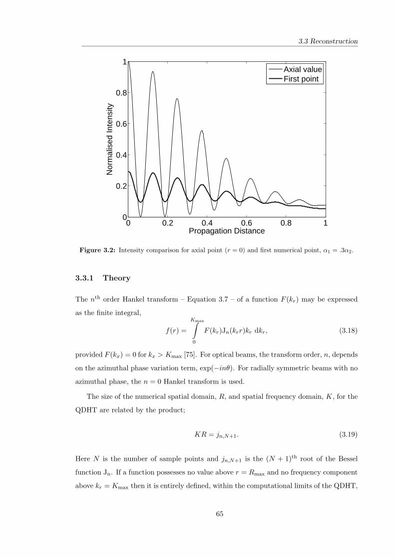
3.3 Reconstruction
0 0.2 0.4 0.6 0.8 10
0.2
0.4
0.6
0.8
1
Propagation Distance
Nor
mal
ised
Inte
nsity
Axial valueFirst point
Figure 3.2: Intensity comparison for axial point (r = 0) and first numerical point, α1 = .3α2.
3.3.1 Theory
The nth order Hankel transform – Equation 3.7 – of a function F (kr) may be expressed
as the finite integral,
f(r) =
Kmax∫0
F (kr)Jn(krr)kr dkr, (3.18)
provided F (kx) = 0 for kx > Kmax [75]. For optical beams, the transform order, n, depends
on the azimuthal phase variation term, exp(−inθ). For radially symmetric beams with no
azimuthal phase, the n = 0 Hankel transform is used.
The size of the numerical spatial domain, R, and spatial frequency domain, K, for the
QDHT are related by the product;
KR = jn,N+1. (3.19)
Here N is the number of sample points and jn,N+1 is the (N + 1)th root of the Bessel
function Jn. If a function possesses no value above r = Rmax and no frequency component
above kr = Kmax then it is entirely defined, within the computational limits of the QDHT,
65

Chapter 3: Hankel-Based Adaptive Radial Propagator
by N samples when
jn,N < KmaxRmax ≤ jn,N+1. (3.20)
No additional precision is gained by increasing N above this value [74, 75]. This radial
space-bandwidth product limit is analogous to the familiar Shannon-Nyquist sampling
theorem. Of course, no function may strictly be simultaneously band-limited in both
space and frequency space. In practice, however, it may be stated that the function is
space-bandwidth limited by numerical noise when the function possesses no value above
numerical precision outside these bounds.
It can be shown [82, 83] that functions sampled on the grid rn,p, where rn,p = jn,p/K,
may be reconstructed at an arbitrary point r as;
f0(r) =∞∑
p=1
f(rn,p)Sk(r), (3.21)
with the sampling kernel
Sk(r) =2rn,pJn(Kr)
K(r2n,p − r2)Jn+1(Krn,p)
. (3.22)
From this the function f(rn,p) may be reconstructed as f0(r) at any arbitrary point
in r, including r = 0 provided the function is sampled on the non-uniform grid rn,p.
This reconstruction method is generalised for any Hankel transform of order n but is only
considered here in relation to the QDHT for which n ∈ Z.
Additionally, points which do not lie at r = 0, but do not coincide with a point on
rn,p either, may be of interest. For a single point it may be reasonable to simply adjust
the number of sample points such that the desired point now lies on rn,p. In general
however this may not be appropriate. Consider for example the comparison of a radially
propagated beam with data sampled on grid defined for use with the FFT. In this situation
the uneven separation of rn,p is not compatible with the even spacing of the FFT.
The application of Eq. (3.21) is not limited to the study of beams for which the axis
is the main point of interest. Because this equation is generalised to Hankel transforms of
order n it is possible to study the propagation of beams possessing angular momentum.
For such vortex beams the field on axis will always be zero, however it is often the near-
axial points which are of interest. Using Eq. (3.21) it would be possible to model these
66

3.3 Reconstruction
beams efficiently using a minimal number of sample points and then reconstruct the near-
axial region – or any region of interest – to a high degree of accuracy. It is also possible
to compare the propagation of beams with differing azimuthal phase where the sample
points would lie on the grids rn1,p and rn2,p where n1 6= n2. This generalised interpolation
should allow mixing of various techniques such as resampling linear combinations of vortex
beams on to grids suitable for finite differences or 2D FFT grids without the addition of
significant numerical artifacts.
3.3.2 Analysis
To analyse the reconstruction error, five beam-like functions with different rates of spectral
convergence [84] are tested. The reconstruction errors of these functions, for increasing
sample densities, are shown in Figure 3.3. The forms, and rates of convergence in frequency
space, of the test functions are given in Table 3.2. These are compared against the same
functions reconstructed from a 2D Cartesian grid of size N2FFT using the cardinal series
[82] in Figure 3.3b. Such reconstruction is compatible with the grid spacing required for
the FFT.
The error was determined by comparing the function f0(r), reconstructed from the
sampled function f(rn,p), against the analytic form of the test function f(r). From this
we determine the maximum error,
ε∞ = ||f0(r)− f(r)||∞. (3.23)
This error was estimated by sampling r over a large number of points linearly spaced over
the region 0 ≤ r ≤ Rmax. For Figure 3.3a 1000 points were used to determine ε∞ and for
Figure 3.3b the function was reconstructed onto 2D grid of 1000× 1000 points.
The reconstruction error is introduced when the function is not effectively space-
bandwidth limited. Therefore the error due to reconstruction is expected to fall, with
increasing sample density, at the same rate as the function. The larger noise floor in Fig-
ure 3.3a when compared to the 2D FFT is caused by the limited precision to which the
Bessel function and its roots may be calculated. To reach a nominal accuracy of 10−10 in
the reconstruction of a Gaussian function requires N = 95 points using Eq. (3.21) and
NFFT = 176 along one dimension (30976 points in total) using the cardinal series. For the
67

Chapter 3: Hankel-Based Adaptive Radial Propagator
0 200 400 600 800
10−15
10−10
10−5
100
Number of sample points
ǫ∞
12345
Noise Floor
(a) Reconstruction with Eq. (3.21)
0 200 400 600 800
10−15
10−10
10−5
100
Number of sample points (NFFT
)
ǫ∞
12345
Noise Floor
(b) Two dimensional reconstruction with cardinal series
Figure 3.3: Reconstruction error for test functions shown in Table 3.2.
68

3.3 Reconstruction
sech function the same precision is reached when N = 314 and NFFT = 566.
Table 3.2: Typical beam-like functions.Index on Fig 3.3a Function Convergence Name1 sech(r) Geometric Sech2 exp(−r2) Super Geometric Gaussian3 H(r)−H(1− r) Sub Geometric Pupil4 exp(−r2)J0(r) Super Geometric Bessel-Gauss5 r exp(−r2)L1
0(2r2) exp(iφ) Super Geometric Laguerre-Gauss
The rate of convergence for a function in the real or spectral domain may be gener-
alised into two forms, geometric and algebraic. Functions exhibiting algebraic convergence,
converge as f(r) ∼ r−q for any positive q; geometric convergence is typified by the rate
f(r) ∼ exp(−rp). This can be subdivided into Super- (p > 1), Simple- (p = 1) and
Sub-Geometric (p < 1).
The Gaussian, Bessel-Gauss and Laguerre-Gauss functions all exhibit a super-geometric
rate of convergence in both space and frequency space and are consequently excellent can-
didates for representation by spectral techniques of this form. This results in a rapid
convergence in the reconstruction error on a noise floor. The off-axis maximum in the
Bessel-Gauss reconstruction error may be simply attributed to the off-axis nature of the
Bessel-Gauss spectrum. Although the sech function converges at a geometric rate in both
domains, the reconstruction error still quickly converges on a noise floor.
Finally a step function is considered, which is effectively a pupil due to the radial
symmetry. The spectrum of a step function converges at an algebraic rate. This poor rate
of convergence means that the function is never well sampled. As a result we see that the
error also decreases algebraically ∼ O(N−2). To reduce the error to 10−10, significantly
greater precision than is often of experimental interest, would require 105 sample points
for the QDHT. Therefore the reconstruction technique, and indeed spectral techniques in
general, are less suited to functions of this form. The 2D reconstruction of this function
using the cardinal series results in a constantly large maximum error [Figure 3.3b] as the
pupil function is poorly represented by a Cartesian grid.
To assess the accuracy and speed of this reconstruction technique, when combined with
a beam propagation model, axial values obtained in four ways are compared. First 2D
FFT technique for which the axial value will already lie on the sample grid is used; second
the QDHT in combination with the reconstruction technique described above is used; third
69

Chapter 3: Hankel-Based Adaptive Radial Propagator
the QDHT is used under the assumption that r = 0 ' r0,1; finally the oversampled QDHT
is used so that r0,1 is much closer to r = 0.
To assess the accuracy and efficiency of this technique when combined with a simple
beam propagation model, a Gaussian beam profile is propagated over one Rayleigh length
from its waist using 4000 steps for each technique. The reconstructed value on axis,
f0(r = 0, z) is compared to the analytic value f(r = 0, z) and the maximum error for the
axial point is determined from
εz∞ = ||f0(0, z)− f(0, z)||∞. (3.24)
Due to the radial symmetry of the Gaussian beam, the n = 0 QDHT transform is
used. To make the most efficient use of each transform the total number of sample points
N , given in Table 3.3, was chosen so that the beam is sampled just above the numerical
limit of the space-bandwidth product through the entire propagation. For the 2D FFT
N was padded from the observed Nyquist minimum of N = 134 points to 135, a product
of small prime numbers (3, 3, 3, 5) to make optimal use of the FFTW routine [77], the 2D
FFT will therefore have N2 points. This is approximately twice as fast as padding to the
nearest power of two (256). As such the 2D FFT method is presented in the best possible
light.
Table 3.3: Accuracy of field on axis and relative speed for each method.Method N Time log10(εz
∞)2D FFT 135 100 −13QDHT 62 2.3 −2QDHT (reconstructed) 62 2.5 −12QDHT (oversampled) 4000 2000 −6
The speed for each technique, shown in Table 3.3, has been normalised relative to the
2D FFT which is 100 time units. The QDHT, without reconstruction, is the fastest but
there is a considerable error in the value of the r = 0 point, consistent with Figure 3.2.
The QDHT technique, with reconstruction at r = 0, exhibits negligible additional time
penalty but vastly improves the accuracy of the axial value. Increasing the number of
sample points in the QDHT causes the time to increase as N2 and only reduces the error
by N−2, consequently the oversampled field only sees a small improvment in accuracy.
Clearly to approach the accuracy of the QDHT technique with reconstruction, or indeed
70

3.4 Adaptive Step Length
the naive 2D FFT, oversampling the QDHT is an unwise proposition.
3.4 Adaptive Step Length
The most simple way of implementing the split-step method is to use a constant step
length. By constructing a dynamic step length the model may advance efficiently in
regions of low nonlinearity and then take much finer steps as the nonlinearity increases.
This adaptive step length is constructed using a local error technique.
3.4.1 Theory
The local error may be defined as the error between the calculated field, um, and the true
solution, u
δ =||um − u||2||u||2
. (3.25)
However, the true solution to the beam is, of course, unknown.
Since the accuracy will vary with the step length, it is possible to compare the field to
another field calculated using shorter steps. If uc is the course solution, obtained using one
symmetrised split-step over a distance ∆z and uf is the fine solution, calculated using two
symmetrised split-steps each of length ∆z/2 then the local relative error may be written
as
δr =||uf − uc||2||u− f ||2
. (3.26)
This error may be compared, after each step, against a tolerance, G and a decision is made
about the step length. If the error is to large, the step size is reduced, and if the error is
too small the step size is increased.
3.4.2 Implementation
This local relative error, shown in Figure 3.4 varies as O(∆z3). A scheme is then devised
whereby the local relative error is maintained in a band between G/2 < δr < G. Supposing
the initial step length causes the error to fall within this bound then one of two outcomes
is likely: either the beam is of low power and linear diffraction will dominate or the
beam is of sufficient power that nonlinear self-focusing will dominate. In the case of
predominantly linear diffraction the beam intensity will drop resulting in a smaller error
71

Chapter 3: Hankel-Based Adaptive Radial Propagator
10−6
10−4
10−2
100
102
10−10
10−5
100
105
1010
Propagation distance (z/z0)
Err
or
(δ/G
)
Figure 3.4: Local relative error (δ) variation with step-length (solid), compared to O(∆z3)estimate (dashed).
from the symmetrised split-step. This will cause the local relative error to also drop,
eventually falling below the lower threshold. The step length may then be increased.
Since the local relative error scales as O(∆z3) it is sensible to assume that the largest
increment of ∆z that may be made is 21/3∆z. In the case of nonlinear self-focusing the
intensity of the beam will begin to locally increase, causing an increase in the symmetrised
split-step error. Once the local relative error reaches G then the step size is reduced to
2−1/3∆z such that the error will be returned to the lower bound. If the error is in excess
of 2G then there is considered to be too much error present in the symmetrised split-step,
the iteration is discarded and the step length set to ∆z/2; this is only likely to occur when
the beam is beyond the threshold for collapse.
In the situation where the initial step length causes the relative local error to fall
outside of the desired band, the step size is treated in exactly the same manner and the
error will eventually converge on the desired error band. If the initial error is greatly in
excess of the desired region then a better approximation may be made
∆z =(ε1
G
)−1/3∆z1, (3.27)
where ε1 is the relative local error corresponding to the initial step length, ∆z.
72
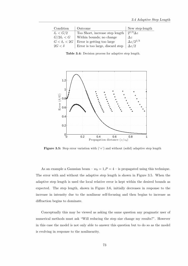
3.4 Adaptive Step Length
Condition Outcome New step-lengthδr < G/2 Too Short, increase step length 21/3∆zG/2δr < G Within bounds; no change ∆z
G < δr < 2G Error is getting too large ∆z/21/3
2G < δ Error is too large, discard step ∆z/2
Table 3.4: Decision process for adaptive step length.
0 0.2 0.4 0.6 0.8 10
0.2
0.4
0.6
0.8
1
1.2
Propagation distance (z/z0)
Err
or
(δ/G
)
Figure 3.5: Step error variation with (‘+’) and without (solid) adaptive step length
As an example a Gaussian beam – w0 = 1,P = 4 – is propagated using this technique.
The error with and without the adaptive step length is shown in Figure 3.5. When the
adaptive step length is used the local relative error is kept within the desired bounds as
expected. The step length, shown in Figure 3.6, initially decreases in response to the
increase in intensity due to the nonlinear self-focusing and then begins to increase as
diffraction begins to dominate.
Conceptually this may be viewed as asking the same question any pragmatic user of
numerical methods must ask “Will reducing the step size change my results?”. However
in this case the model is not only able to answer this question but to do so as the model
is evolving in response to the nonlinearity.
73

Chapter 3: Hankel-Based Adaptive Radial Propagator
0 0.2 0.4 0.6 0.8 1
0.5
1
1.5
2
2.5
3
3.5
4
Propagation distance (z/z0)
Ste
pLength
(∆z/∆
z0)
0 0.2 0.4 0.6 0.8 10
0.2
0.4
0.6
0.8
1
1.2
1.4
Axia
lIn
tensi
ty(I
/I0)
Figure 3.6: Step length (solid) and intensity on axis (dashed)
3.4.3 Increased accuracy
The primary motivation for implementing a dynamic step length is to improve the effi-
ciency of the propagation method. It is not necessary to guess the step length and then
repeat the simulation to improve the estimate. Calculating both the coarse and fine so-
lutions requires more calls the QDHT routine – 11 QDHTs to calculate both the coarse
and fine solution and 8 to calculate the fine solution alone; however, calculating both the
coarse uc and fine uf solutions may be used to improve the accuracy of the model. Given
the symmetrised split-step method is third-order accurate, the coarse solution must be
related to the true solution, u, as
uc = u + C∆z3 + O(∆z4), (3.28)
for some constant C. The same relation for the fine solution is given by;
uf = u + 2C
(∆z
2
)3
+ O(∆z4). (3.29)
By taking the appropriate linear combinations of Equation 3.29 and Equation 3.28 it is
possible to construct an equation for which the leading error is of order O(∆z4) [57]
u4 =43uf −
13uc = u + O(∆z4). (3.30)
74

3.5 Adaptive Grid Size
Technique Time Global accuracyStatic 100 O(∆z2)Improved accuracy 160 O(∆z3)Dynamic 20 O(∆z3)
Table 3.5: Speed and global accuracy for adaptive step length
This means that although the relative local error technique requires more calls to the FFT
routine; not only is the step size able to vary – making optimal use of the step length – each
iteration may be evaluated to a higher degree of accuracy. Alternatively the model may
be run more efficiently but to the same degree of accuracy by using longer step lengths.
3.4.4 Speed
As already mentioned, the dynamic stepping method shown here requires nearly 50%
more calls to the QDHT routine. However, this may be offset by taking longer steps when
possible. As an example a moderately high power Gaussian beam – w0 = 1, P = 4 – is
then propagated with the adaptive step length. This beam is the propagated using three
methods. First the beam is propagated using the static split step method to serve as a
benchmark with which the other two techniques may be compared. Then the beam is
propagated using a static split step method but using a coarse step of 2∆z to improve
accuracy at the expense of time taken. Finally the beam is propagated using the dynamic
step length technique. The time taken to propagate the beam over one diffraction length is
given in normalised units of time in Table 3.5. Even though the dynamic method requires
more calls to the transform routine it presents a considerable improvement in both time
and accuracy over the static step length method. Additionally the use of an adaptive step
length removes the need to determine a suitable step length in advance, allowing different
problems to be iterated in faster succession.
3.5 Adaptive Grid Size
As was discussed in Section 3.3 the most efficient method to propagate a beam is by sam-
pling as close as possible to the space-bandwidth product. However, as a beam propagates
this position will vary, either through linear diffraction or the introduction of additional
transverse spatial frequencies due to the nonlinear interaction. If the grid is only just big
enough for the initial field then subsequent iterations may become aliased. To prevent this,
75

Chapter 3: Hankel-Based Adaptive Radial Propagator
the field is typically vastly over-specified so that the beam has sufficient space to diffract
into – in both real and frequency space. This technique is inefficient as a considerable
amount of the numerical grid is not used for most of the propagation.
Previous methods for adapting the numerical grid in response to the beam propagation
have centred around the rescaling of the grid spacing [78]. Such methods still require the
initial grid to be large enough to fully define the beam at the maximum space-bandwidth
product. This is justified in the setting of [78] – where the authors are primarily interested
in the blowup and collapse dynamics of Gaussian beams.
For beams below the self-focusing threshold the combination of linear diffraction and
the nonlinear “spreading” of transverse frequencies requires a technique which is more
flexible. The method introduced here is based on an adaptive grid technique from a
2D FFT based technique. This is adapted, for the first time, to radial co-ordinates and
implemented using the QDHT.
The numerical grid is split into two regions, the beam area and the guard area. As the
beam propagates, the power in the guard band is monitored. Once this passes a predefined
threshold the beam is considered to be aliased. The field is reverted back to a previous
copy which is not aliased, usually the previous step. The guard band is then incorporated
into the beam area and a new guard band is padded onto the beam. This performed in
both real and transverse frequency space.
Figure 3.7: Guard band (red) and numerical band (black) for three successive grid sizes
3.5.1 Resizing in the QDHT
Increasing the grid density in the FFT case is trivial; however in the case of the QDHT
it is not so immediately obvious how to proceed. In the case where a beam, sampled on
N1 points, is considered aliased the field may be padded as follows. The new number of
sample points is calculated, N2 = f(N1), where f is a monotonic function; this is then used
to recalculate the value of Rmax from Rmax = j0,N2+1/Kmax. Next the position arrays, rn
and kr,n are re-allocated. Finally the field array is padded with (N2 − N1) zeroes. Once
76
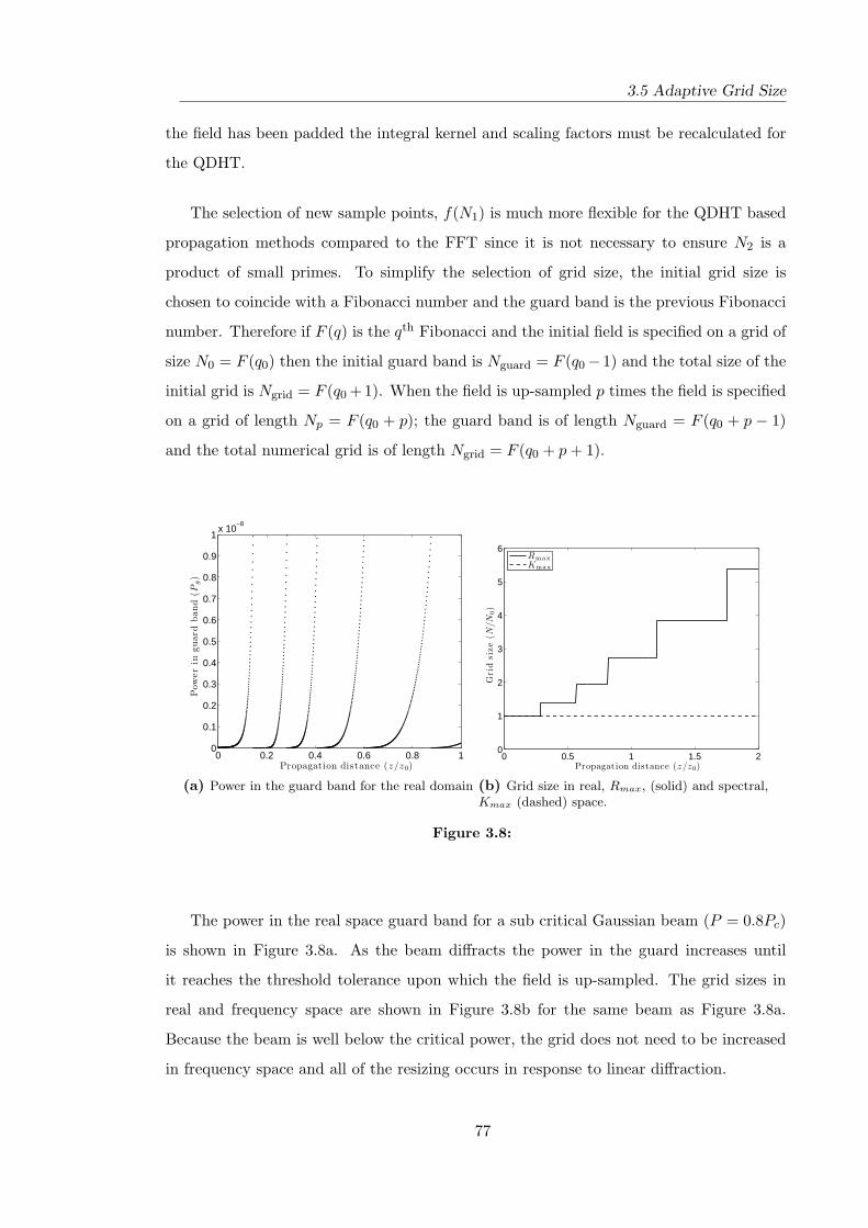
3.5 Adaptive Grid Size
the field has been padded the integral kernel and scaling factors must be recalculated for
the QDHT.
The selection of new sample points, f(N1) is much more flexible for the QDHT based
propagation methods compared to the FFT since it is not necessary to ensure N2 is a
product of small primes. To simplify the selection of grid size, the initial grid size is
chosen to coincide with a Fibonacci number and the guard band is the previous Fibonacci
number. Therefore if F (q) is the qth Fibonacci and the initial field is specified on a grid of
size N0 = F (q0) then the initial guard band is Nguard = F (q0− 1) and the total size of the
initial grid is Ngrid = F (q0 +1). When the field is up-sampled p times the field is specified
on a grid of length Np = F (q0 + p); the guard band is of length Nguard = F (q0 + p − 1)
and the total numerical grid is of length Ngrid = F (q0 + p + 1).
0 0.2 0.4 0.6 0.8 10
0.1
0.2
0.3
0.4
0.5
0.6
0.7
0.8
0.9
1x 10
−8
Propagation distance (z/z0)
Pow
er
inguard
band
(Pg)
(a) Power in the guard band for the real domain
0 0.5 1 1.5 20
1
2
3
4
5
6
Propagation distance (z/z0)
Gri
dsi
ze
(N/N
0)
Rmax
Kmax
(b) Grid size in real, Rmax, (solid) and spectral,Kmax (dashed) space.
Figure 3.8:
The power in the real space guard band for a sub critical Gaussian beam (P = 0.8Pc)
is shown in Figure 3.8a. As the beam diffracts the power in the guard increases until
it reaches the threshold tolerance upon which the field is up-sampled. The grid sizes in
real and frequency space are shown in Figure 3.8b for the same beam as Figure 3.8a.
Because the beam is well below the critical power, the grid does not need to be increased
in frequency space and all of the resizing occurs in response to linear diffraction.
77
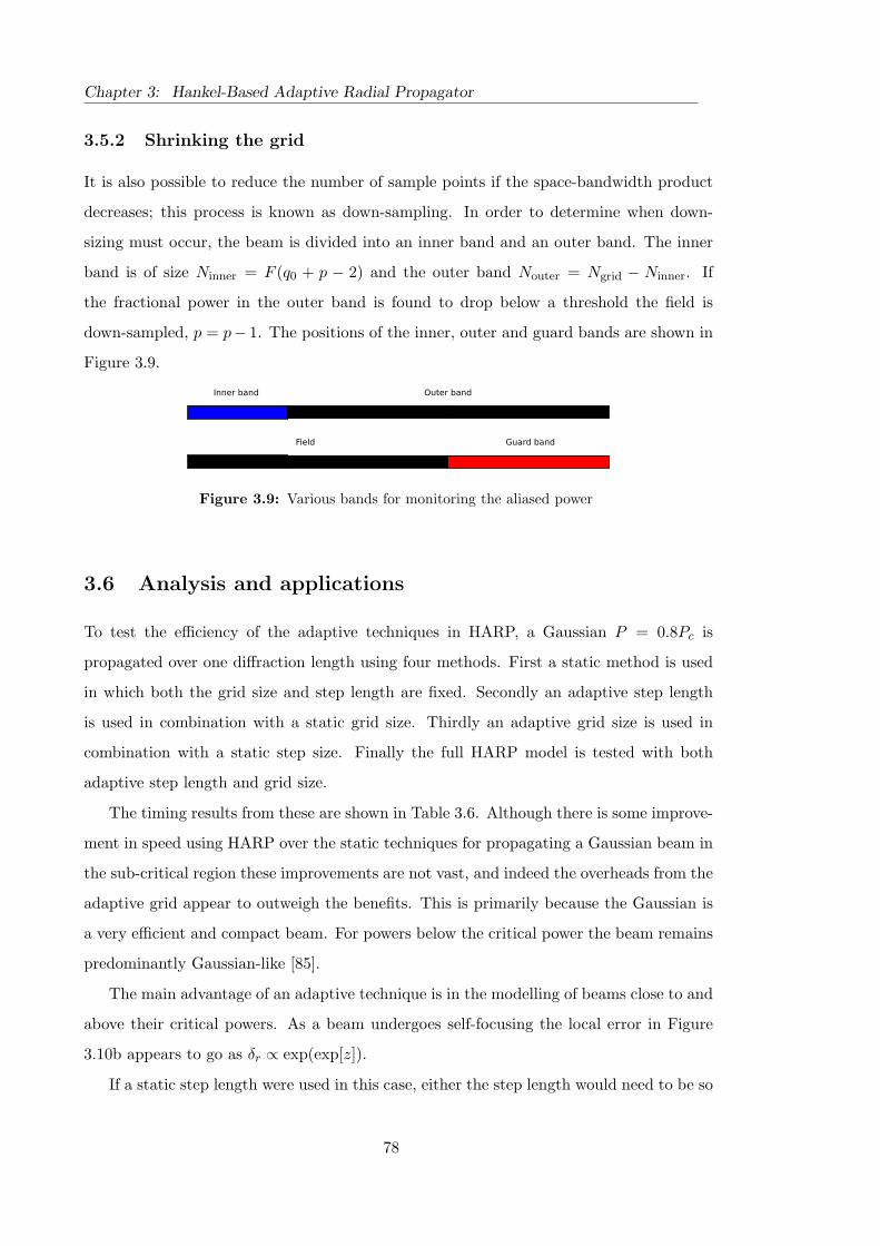
Chapter 3: Hankel-Based Adaptive Radial Propagator
3.5.2 Shrinking the grid
It is also possible to reduce the number of sample points if the space-bandwidth product
decreases; this process is known as down-sampling. In order to determine when down-
sizing must occur, the beam is divided into an inner band and an outer band. The inner
band is of size Ninner = F (q0 + p − 2) and the outer band Nouter = Ngrid − Ninner. If
the fractional power in the outer band is found to drop below a threshold the field is
down-sampled, p = p− 1. The positions of the inner, outer and guard bands are shown in
Figure 3.9.
Figure 3.9: Various bands for monitoring the aliased power
3.6 Analysis and applications
To test the efficiency of the adaptive techniques in HARP, a Gaussian P = 0.8Pc is
propagated over one diffraction length using four methods. First a static method is used
in which both the grid size and step length are fixed. Secondly an adaptive step length
is used in combination with a static grid size. Thirdly an adaptive grid size is used in
combination with a static step size. Finally the full HARP model is tested with both
adaptive step length and grid size.
The timing results from these are shown in Table 3.6. Although there is some improve-
ment in speed using HARP over the static techniques for propagating a Gaussian beam in
the sub-critical region these improvements are not vast, and indeed the overheads from the
adaptive grid appear to outweigh the benefits. This is primarily because the Gaussian is
a very efficient and compact beam. For powers below the critical power the beam remains
predominantly Gaussian-like [85].
The main advantage of an adaptive technique is in the modelling of beams close to and
above their critical powers. As a beam undergoes self-focusing the local error in Figure
3.10b appears to go as δr ∝ exp(exp[z]).
If a static step length were used in this case, either the step length would need to be so
78

3.6 Analysis and applications
0 0.5 1 1.5 20
1
2
3
4
5
6
7
8
9
10
11
Propagation distance (z/z0)
Gri
dsi
ze
RmaxKmax
(a) Grid sizes for a Gaussian beam
0 0.2 0.4 0.6 0.8 110
−1
100
101
102
103
104
Propagation distance (z/z0)
Local
Err
or
(δ/G
)-
Sta
tic
step
length
0 0.2 0.4 0.6 0.8 10.1
0.2
0.3
0.4
0.5
0.6
0.7
0.8
0.9
1
1.1
Local
Err
or
(δ/G
)-
Adapti
ve
step
length
StaticAdaptive
(b) Relative local error with (blue ‘x’) and without (red line) adaptive step length for a Gaussianbeam P > Pc
Figure 3.10:
79
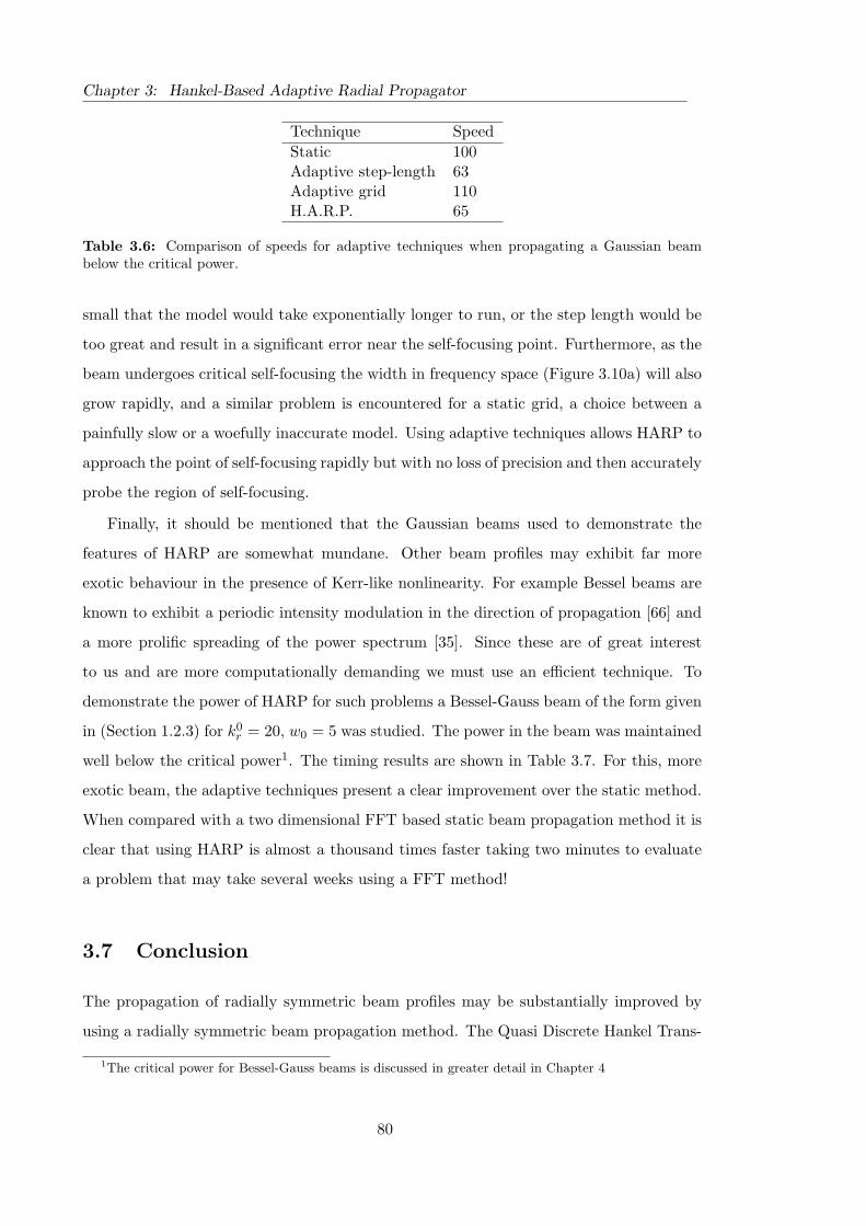
Chapter 3: Hankel-Based Adaptive Radial Propagator
Technique SpeedStatic 100Adaptive step-length 63Adaptive grid 110H.A.R.P. 65
Table 3.6: Comparison of speeds for adaptive techniques when propagating a Gaussian beambelow the critical power.
small that the model would take exponentially longer to run, or the step length would be
too great and result in a significant error near the self-focusing point. Furthermore, as the
beam undergoes critical self-focusing the width in frequency space (Figure 3.10a) will also
grow rapidly, and a similar problem is encountered for a static grid, a choice between a
painfully slow or a woefully inaccurate model. Using adaptive techniques allows HARP to
approach the point of self-focusing rapidly but with no loss of precision and then accurately
probe the region of self-focusing.
Finally, it should be mentioned that the Gaussian beams used to demonstrate the
features of HARP are somewhat mundane. Other beam profiles may exhibit far more
exotic behaviour in the presence of Kerr-like nonlinearity. For example Bessel beams are
known to exhibit a periodic intensity modulation in the direction of propagation [66] and
a more prolific spreading of the power spectrum [35]. Since these are of great interest
to us and are more computationally demanding we must use an efficient technique. To
demonstrate the power of HARP for such problems a Bessel-Gauss beam of the form given
in (Section 1.2.3) for k0r = 20, w0 = 5 was studied. The power in the beam was maintained
well below the critical power1. The timing results are shown in Table 3.7. For this, more
exotic beam, the adaptive techniques present a clear improvement over the static method.
When compared with a two dimensional FFT based static beam propagation method it is
clear that using HARP is almost a thousand times faster taking two minutes to evaluate
a problem that may take several weeks using a FFT method!
3.7 Conclusion
The propagation of radially symmetric beam profiles may be substantially improved by
using a radially symmetric beam propagation method. The Quasi Discrete Hankel Trans-
1The critical power for Bessel-Gauss beams is discussed in greater detail in Chapter 4
80
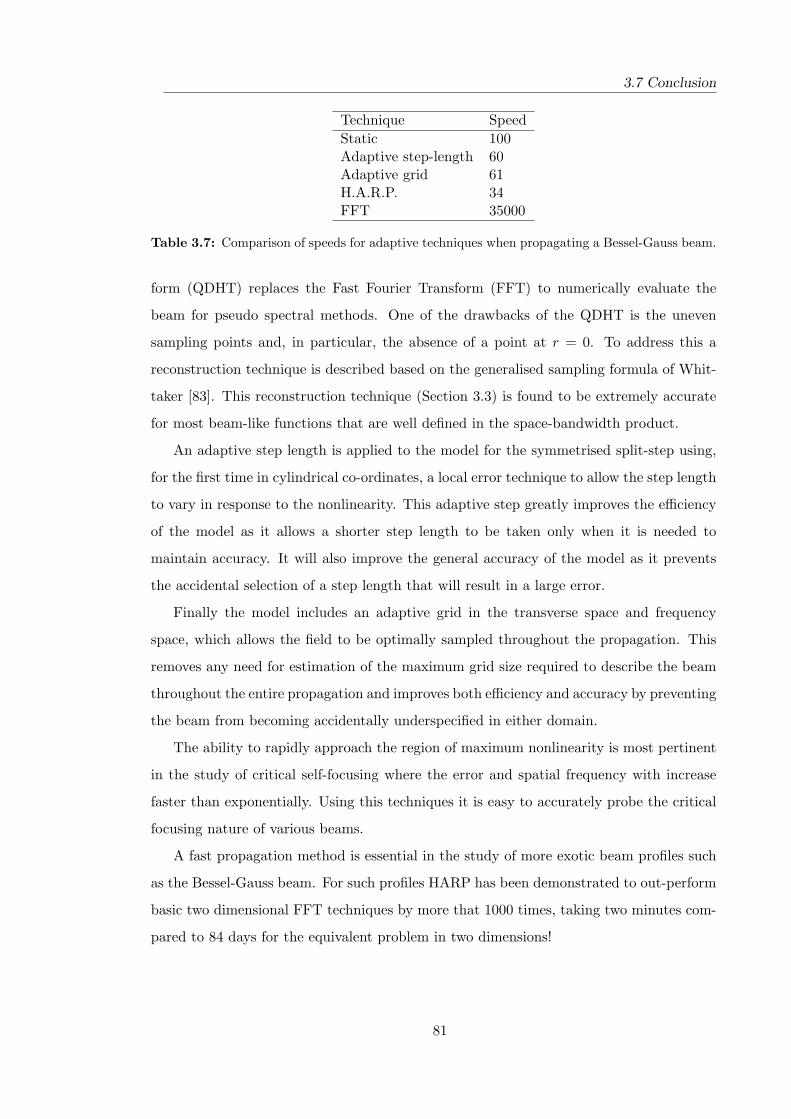
3.7 Conclusion
Technique SpeedStatic 100Adaptive step-length 60Adaptive grid 61H.A.R.P. 34FFT 35000
Table 3.7: Comparison of speeds for adaptive techniques when propagating a Bessel-Gauss beam.
form (QDHT) replaces the Fast Fourier Transform (FFT) to numerically evaluate the
beam for pseudo spectral methods. One of the drawbacks of the QDHT is the uneven
sampling points and, in particular, the absence of a point at r = 0. To address this a
reconstruction technique is described based on the generalised sampling formula of Whit-
taker [83]. This reconstruction technique (Section 3.3) is found to be extremely accurate
for most beam-like functions that are well defined in the space-bandwidth product.
An adaptive step length is applied to the model for the symmetrised split-step using,
for the first time in cylindrical co-ordinates, a local error technique to allow the step length
to vary in response to the nonlinearity. This adaptive step greatly improves the efficiency
of the model as it allows a shorter step length to be taken only when it is needed to
maintain accuracy. It will also improve the general accuracy of the model as it prevents
the accidental selection of a step length that will result in a large error.
Finally the model includes an adaptive grid in the transverse space and frequency
space, which allows the field to be optimally sampled throughout the propagation. This
removes any need for estimation of the maximum grid size required to describe the beam
throughout the entire propagation and improves both efficiency and accuracy by preventing
the beam from becoming accidentally underspecified in either domain.
The ability to rapidly approach the region of maximum nonlinearity is most pertinent
in the study of critical self-focusing where the error and spatial frequency with increase
faster than exponentially. Using this techniques it is easy to accurately probe the critical
focusing nature of various beams.
A fast propagation method is essential in the study of more exotic beam profiles such
as the Bessel-Gauss beam. For such profiles HARP has been demonstrated to out-perform
basic two dimensional FFT techniques by more that 1000 times, taking two minutes com-
pared to 84 days for the equivalent problem in two dimensions!
81

Chapter 3: Hankel-Based Adaptive Radial Propagator
82

Chapter 4
Critical self-focusing
In Section 2.2 the concept of critical self-focusing was introduced; for high power beams
the intensity introduces a lens like refractive index change within the material. If this
focusing outweighs the linear diffraction the intensity will continue to grow and ‘collapse’
inwardly. This chapter deals with a more rigorous interpretation of critical self-focusing
based on the nonlinear Schrodinger equation (NSE). Precise definitions are provided for
the different forms of self-focusing and sufficient conditions are stated where available.
In the absence of sufficient conditions, the beam fate must be tested numerically using a
model such as HARP.
While much work has been conducted on common beams such as the Gaussian [86]
there is little accessible work looking at the beam fate for more exotic profiles such as the
Bessel-Gauss beam. This chapter reviews the work on the Gaussian and Townes beams
and then begins to explore self-focusing behaviour for the Bessel-Gauss beam.
4.1 Self-focusing
In Section 2.3 a nonlinear Schrodinger equation was derived to describe the propagation
of light in a Kerr-like nonlinear medium. This form of nonlinear Schrodinger equation is
known as a power nonlinearity [87] and may be written in a slightly more general form as
i∂u
∂z+∇2
⊥u + |u|2σu = 0, (4.1)
83

Chapter 4: Critical self-focusing
where u = u(x, z), x ∈ RD, z ∈ R+ and D is the number of transverse dimensions.
In the region where σ < 2/D then the beam may not critically self-focus; therefore,
critical self-focusing may not occur in an idealised fiber for which σ = 1, D = 1. In
the case where σ ≥ 2/D, Equation 4.1 may result in singularity formation in u. As the
lower boundary to this condition, σ = 2/D is considered the critical case. Therefore, the
nonlinear Schrodinger equation describing the propagation of a two dimensional initial
field, σ = 1, D = 2 is referred to as the critical nonlinear Schrodinger equation [88].
Considerable work has been undertaken to understand the fate of beams propagated in
this and similar forms of the nonlinear Schrodinger equation [86, 87, 88]. For the purposes
of this chapter two dimensional initial conditions are considered in a Kerr-like medium.
4.1.1 Catagorising self-focusing
It is commonly stated that a beam will self-focus above a threshold power Pc [59, 60]
– while this statement is not untrue the precise meaning of “self-focus” is rather vague.
Critical self-focusing is generally considered to be the point at which linear diffraction no
longer outweighs the nonlinear focusing, it is assumed that the beam continually focuses,
implying the beam waist will tend to zero as the intensity simultaneously tends to infinity.
More generally it has been shown [88] that the beam fate may be divided into three
categories, Blowup (BU) whereby the field exhibits a singular value in a finite distance,
Collapse (CL) where BU occurs and the beam waist tends to zero and Global Existence
(GE) when neither of these occur. In order to study general beam profiles rather than
the well-studied case of the Gaussian it is necessary to precisely define these behaviours
as follows.
Definition 4.1 (Blowup). The L2 norm of the gradient of the field tends to infinity,
||∇u||2 → ∞ [88]. This is equivalent to the maximum field value also tending to infinity
max(|u|) →∞ and the second moment of power spectrum density also tending to infinity.
Definition 4.2 (Collapse). Collapse is a subset of blowup [88] where the second moment
of beam intensity (beam width) tends to zero.
Definition 4.3 (Global existence). Global existence occurs when the beam exists for all
space and may be defined as the absence of blowup.
84

4.1 Self-focusing
The three beam fates defined above represent all possible outcomes from the NSE. If
the universal set, U , is defined as all possible beam fates then global existence (GE) is the
complement of blowup (BU),
GE = BUc, (4.2)
and collapse (CL) is a subset of blowup
CL ⊆ BU. (4.3)
Now that these definitions and relationships have been established it is possible to begin
determining sufficient conditions for each region.
4.1.2 Invariants
It may be shown [87] that solutions to the NSE are subject to the following conserved
quantities, power
P = ||u||22, (4.4)
and the Hamiltonian
H0 = ||∇u||22 −12||u||44. (4.5)
Because these two quantities are invariant over propagation it is convenient to define
conditions for the GE, BU and CL in terms of them, in particular power which may be
easily measured in a laboratory setting.
4.1.3 Townes soliton
The NSE (Equation 4.1) permits stationary solutions of the form
u(r, z) = Φ(r; kz) exp(ikzz), (4.6)
where kz ∈ R and for σ = 1 Φ ∈ R. By substituting Equation 4.6 into the NSE (Equation
4.1) an ODE may be written for Φ,
∇2⊥Φ− kzΦ + Φ3 = 0. (4.7)
85

Chapter 4: Critical self-focusing
The ground state solution to Equation 4.7 for D = 2 is known as the Townes soliton,
R0(r) = Φ(r, z = 0; kz = 1). (4.8)
This is the solution to Equation 4.7 given ∂rΦ = 0 and Φ(r = ∞) = 0.
The Townes profile, R0 has been shown [88] to have the lowest L2 norm of all stationary
wave solutions to the NSE. The power of this beam profile ||R0||22 has been shown to play
an important role in determining the beam fate.
4.2 Predicting the beam fate
Much of the analytical work on the problem of blowup is contingent on determining con-
ditions that are necessary and sufficient. These terms are reviewed here since they are
subtle but important. A necessary condition must be fulfilled in order for the event to
occur, but does not guarantee that the event will occur; observation of an event implies
that the necessary condition is met. If the necessary condition has been met it does not
imply the event. For example: It is necessary to put water in the glass before drinking
from it. Without filling the glass it is not possible to drink from it.
If a sufficient condition is satisfied then the event will happen but it is still possible
for the event to happen while the condition is unsatisfied: Turning the glass of water
upside-down is sufficient to empty the water from it. The water will empty if the glass is
upside-down but will also empty if drunk through a straw for example.
Finally, a necessary and sufficient condition will trigger an event if and only if the
condition is met: Successfully completing a viva voce and thesis corrections is a necessary
and sufficient condition for obtaining a PhD!
Having established the three possible fates of a beam it is then a question of how to
determine the fate of the beam based on the initial condition.
Theorem 4.1 (Global Existence). It may be shown [88] that, for a two dimensional initial
condition, a sufficient condition for global existence is
||u0||2 < ||R0||2. (4.9)
In other words, if the power of the beam is less than the power of the Townes soliton
86
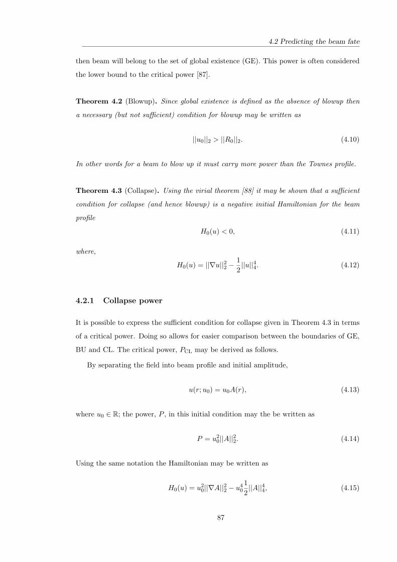
4.2 Predicting the beam fate
then beam will belong to the set of global existence (GE). This power is often considered
the lower bound to the critical power [87].
Theorem 4.2 (Blowup). Since global existence is defined as the absence of blowup then
a necessary (but not sufficient) condition for blowup may be written as
||u0||2 > ||R0||2. (4.10)
In other words for a beam to blow up it must carry more power than the Townes profile.
Theorem 4.3 (Collapse). Using the virial theorem [88] it may be shown that a sufficient
condition for collapse (and hence blowup) is a negative initial Hamiltonian for the beam
profile
H0(u) < 0, (4.11)
where,
H0(u) = ||∇u||22 −12||u||44. (4.12)
4.2.1 Collapse power
It is possible to express the sufficient condition for collapse given in Theorem 4.3 in terms
of a critical power. Doing so allows for easier comparison between the boundaries of GE,
BU and CL. The critical power, PCL may be derived as follows.
By separating the field into beam profile and initial amplitude,
u(r;u0) = u0A(r), (4.13)
where u0 ∈ R; the power, P , in this initial condition may the be written as
P = u20||A||22. (4.14)
Using the same notation the Hamiltonian may be written as
H0(u) = u20||∇A||22 − u4
0
12||A||44, (4.15)
87

Chapter 4: Critical self-focusing
Condition Beam fate||u||2 < ||R0||2 Global ExistenceH0(u) < 0 CollapseOtherwise Indeterminate
Table 4.1: Decision table for sufficient conditions
and the sufficient condition for collapse – Equation 4.12 – may be written as
u20 > 2
||∇A||22||A||44
. (4.16)
Therefore, by substituting Equation 4.16 into Equation 4.14 a sufficient condition for
collapse and hence blowup may be written in terms of a critical power,
PCL = 2||A||22||∇A||22
||A||44. (4.17)
This result is significant because it states that critical power is dependent only on the
profile of the initial condition. This is demonstrated through the analysis of the Gaussian
beam.
4.2.2 Summary of known conditions
The sufficient conditions from theorems 4.1 and 4.3 are summarised in Table 4.1 and the
three possible beam fates are summarised in an Euler-Venn diagram in Figure 4.1. It
should be noted that this diagram does not represent relative sizes in parameter space
such as power and spot size but rather the relation between semi-analytical invariants and
beam fate. In order to determine the relative sizes of each region it is necessary to apply
the sufficient conditions to a specific beam profile. The grey regions represent outcomes
that are not predicted by sufficient conditions and must be determined numerically by
observing close approximations to the definitions of BU, CL and GE in Definition 4.1 -
4.3.
4.3 Numerically determining the beam fate
The regions marked as unknown on Figure 4.1 are not defined by sufficient conditions. To
determine the beam fate in this region, the beam must be numerically evolved. Because
88
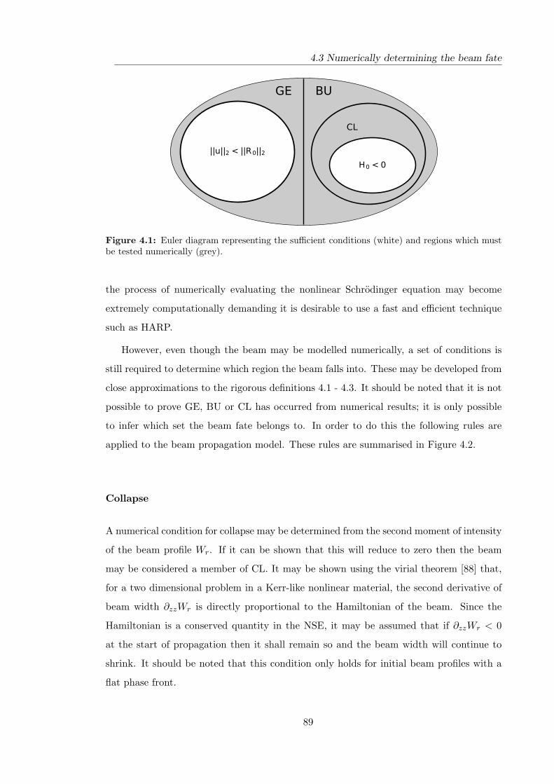
4.3 Numerically determining the beam fate
Figure 4.1: Euler diagram representing the sufficient conditions (white) and regions which mustbe tested numerically (grey).
the process of numerically evaluating the nonlinear Schrodinger equation may become
extremely computationally demanding it is desirable to use a fast and efficient technique
such as HARP.
However, even though the beam may be modelled numerically, a set of conditions is
still required to determine which region the beam falls into. These may be developed from
close approximations to the rigorous definitions 4.1 - 4.3. It should be noted that it is not
possible to prove GE, BU or CL has occurred from numerical results; it is only possible
to infer which set the beam fate belongs to. In order to do this the following rules are
applied to the beam propagation model. These rules are summarised in Figure 4.2.
Collapse
A numerical condition for collapse may be determined from the second moment of intensity
of the beam profile Wr. If it can be shown that this will reduce to zero then the beam
may be considered a member of CL. It may be shown using the virial theorem [88] that,
for a two dimensional problem in a Kerr-like nonlinear material, the second derivative of
beam width ∂zzWr is directly proportional to the Hamiltonian of the beam. Since the
Hamiltonian is a conserved quantity in the NSE, it may be assumed that if ∂zzWr < 0
at the start of propagation then it shall remain so and the beam width will continue to
shrink. It should be noted that this condition only holds for initial beam profiles with a
flat phase front.
89

Chapter 4: Critical self-focusing
Blowup
If the beam is not determined to be collapsing then it will either belong to BU or GE.
To differentiate between these two cases the beam is propagated until the numerical grid
exceeds a maximum size. Once this point is reached a decision must be made. The beam
is deemed to be in BU if the maximum intensity is increasing ∂z max(|u|2) > 0, and width
in frequency space is also increasing ∂zWkr > 0.
4.4 The modified Townes profile
The Townes profile, shown in Figure 4.3, is compared against the sufficient conditions
from Section 4.2. Clearly, since the power in the Townes profile is used as the sufficient
condition for GE then when considered as an initial condition, the Townes profile is exactly
on the border of GE and BU. Furthermore the Hamiltonian of the Townes profile is zero,
H0 = 0, and is therefore exactly on the border of BU and CL. This critical case implies
that the Townes soliton is an unstable initial profile.
If a slight perturbation is added to the Townes profile, such that
u(r) = (1 + ε)R(r), (4.18)
then the beam will either exist globally for ε < 0 or collapse for ε > 0. This supports the
assertion that the Townes profile is unstable initial condition.
The behaviour of the Townes profile, predicted by sufficient conditions is shown in
Figure 4.4. It is important to notice that for the Townes profile will only exhibit global
existence and collapse; there is no region of blowup without collapse. It may be stated
that for this beam
CL = BU. (4.19)
This behaviour is unique for the Townes profile.
4.5 The Gaussian beam revisited
In order to explain the significance of the sufficient conditions for global existence and col-
lapse and place the previous work in context, consider the concrete example of a Gaussian
90

4.5 The Gaussian beam revisited
Figure 4.2: Flow chart for numerically determining self-focusing behaviour.
91
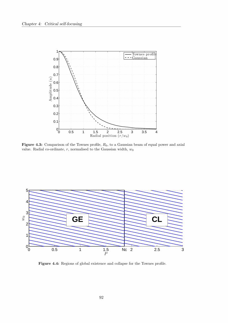
Chapter 4: Critical self-focusing
0 0.5 1 1.5 2 2.5 3 3.5 40
0.1
0.2
0.3
0.4
0.5
0.6
0.7
0.8
0.9
1
Radial position (r/w0)
Am
pli
tude
(u)
Townes profileGaussian
Figure 4.3: Comparison of the Townes profile, R0, to a Gaussian beam of equal power and axialvalue. Radial co-ordinate, r, normalised to the Gaussian width, w0
0 0.5 1 1.5 Nc 2 2.5 30
1
2
3
4
5
P
w0 GE CL
Figure 4.4: Regions of global existence and collapse for the Townes profile.
92

4.5 The Gaussian beam revisited
beam. Since the Gaussian has already been extensively studied in the critical self-focusing
regime [86] it also serves as an excellent candidate for assessing the accuracy of HARP.
The initial condition for the Gaussian beam profile is given by
u(r) = u0 exp(− r2
w02
), (4.20)
where u0 ∈ R and w0 ∈ R. The L2 norm, beam power, may be evaluated analytically and
written as;
||u||2 =14u2
0w20. (4.21)
Equation 4.17 may be also be evaluated analytically to determine a sufficient condition
for collapse in terms of a critical power,
PCL = 2. (4.22)
It is the power alone for any Gaussian beam which will determine whether the beam
is in the sufficient regions for global existence or collapse. Figure 4.5 shows a map of the
sufficient conditions as a function of power and beam waist.
0 0.5 1 1.5 Nc 2 2.5 30
1
2
3
4
5
P
w0
un
kno
wn
GE CL
Figure 4.5: Regions of Global Existence (GE) and Collapse (CL) predicted by sufficient condi-tions. Here Nc is the power of the Townes profile ||R0||22. Note that there is no predicted variationwith beam waist as expected.
The area marked as “unknown” in Figure 4.5 is not defined by the conditions stated
in Section 4.2 and may belong to GE, BU or CL. In order to determine the beam fate in
this region it is necessary to numerically evaluate the NSE using a tool such as HARP
93

Chapter 4: Critical self-focusing
(Chapter 3).
4.5.1 Numerical results
By using HARP with the method for numerically determining regions of GE, BU and CL,
discussed in Section 4.3, the unknown region for the Gaussian beam may be evaluated and
the regions with sufficient conditions confirmed.
The results are shown in Figure 4.6; as with the sufficient conditions for CL and GE,
the numerically determined regions are not obviously dependant on beam waist.
0 0.5 1 1.5 Nc 2 2.5 30
1
2
3
4
5
P
w0
GEBUCL
Figure 4.6: Beam fate determined using HARP, sufficient condition for GE marked as dashedline; cf Figure 4.5.
To determine if HARP is producing accurate results, the boundary for BU is compared
to existing values in Table 4.2. It is interesting to note that the boundary for BU is within
2% of the necessary condition for BU determined from the Townes profile. This is due to
the similarity in the two profiles (Figure 4.3). The value quoted in Boyd [59] is surprisingly
accurate given the simple assumptions made in the derivation. Finally, the critical power
given by Fibich et al. [86] is in agreement with the value obtained from HARP to within
0.02%. This accurate result indicates that the process of modelling using HARP and then
using numerical conditions for CL, BU and GE is suitable for determining the boundaries
between sets of beam fates. Therefore, the fate the Bessel-Gauss beam may be now
investigated with confidence.
94

4.6 Bessel-Gauss beam
Source PowerTownes boundary (Nc) 1.8623Boyd [59] 1.8362Fibich [86] 1.8962HARP 1.8958
Table 4.2: Critical power for blowup of the Gaussian beam
4.6 Bessel-Gauss beam
In this section the fate of the zero-order Bessel-Gauss profile is considered. The Bessel-
Gauss profile in scaled co-ordinates may be written as
uB(r) = u0 exp(− r2
w02
)J0(r), (4.23)
where u0 is the initial amplitude and w0 is the width of the Gaussian envelope.
For the Gaussian beam, varying the beam width had no impact on the critical powers.
This was simply because, no matter what happened to the width, the co-ordinates could
be re-scaled to return the beam to the original form; the problem is scale invariant.
For the Bessel-Gauss beam the width of the Gaussian envelope is relative to the posi-
tions of the zeros of the Bessel function, and so a change in w0 cannot be compensated for
by a re-scaling of co-ordinates as this would alter the periodicity of the Bessel function.
It is therefore expected that this change in profile will break the invariance and lead to
profile dependent effects.
4.6.1 Sufficient conditions
It is possible to determine analytic and semi-analytic sufficient conditions for GE and CL
for the Bessel-Gauss beam as follows.
Global Existence
The power in Equation 4.23 may be written as
||uB||22 = u20
π
2w2
0 exp(−1
4w2
0
)I0
(−1
4w2
0
), (4.24)
95

Chapter 4: Critical self-focusing
where In is the modified Bessel function of order n. Therefore a sufficient condition for
GE may be determined analytically by considering Equation 4.24 in combination with
theorem 4.1.
Collapse
The initial Hamiltonian for the Equation 4.23 may be determined semi-analytically where
||∇uB||22 =12
exp(−w2
0
4
).
[(1 +
w20
4
)I0
(w2
0
4
)+
w20
4I1
(w2
0
4
)], (4.25)
The term ||uB||44 appears to be analytically intractable and is therefore determined through
numerical integration. Although not ideal, this is considerably easier than numerically
integrating the whole expression for the Hamiltonian as it does not require the derivative to
be numerically evaluated. By combining the semi analytic expression for the Hamiltonian
with the expression for power (Equation 4.24) it is possible to predict the critical power
for collapse, PCL.
0 0.5 1 1.5 Nc2 2.5 3 3.5 40
0.5
1
1.5
2
2.5
3
3.5
4
P
w0
Bessel-GaussGaussian
Figure 4.7: Comparison of collapse power for Gaussian and Bessel-Gauss beams
Figure 4.7 shows the position of the critical power for collapse determined through
sufficient conditions. The critical power for a Gaussian beam (determined using the same
method) is also shown for comparison.
Increasing w0 is equivalent to increasing the number of lobes from the Bessel function
96
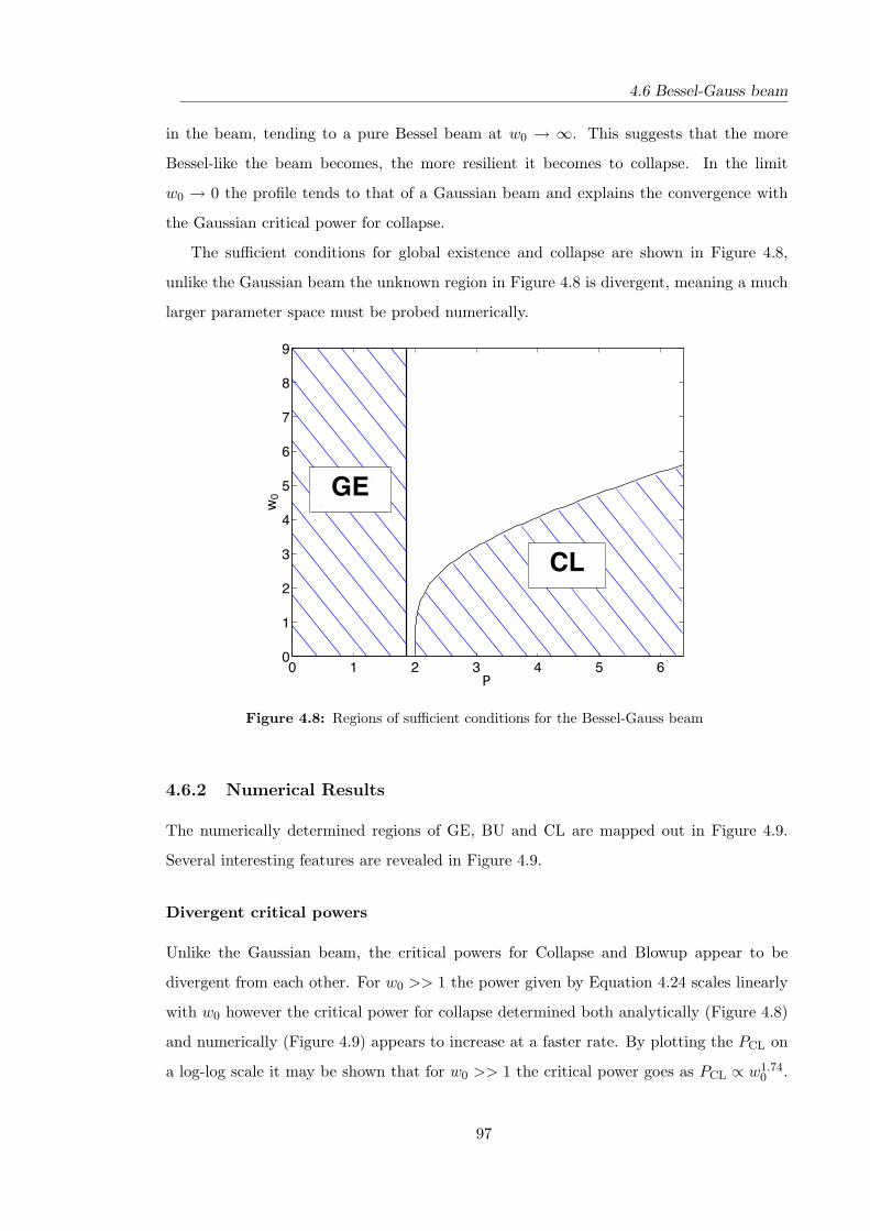
4.6 Bessel-Gauss beam
in the beam, tending to a pure Bessel beam at w0 → ∞. This suggests that the more
Bessel-like the beam becomes, the more resilient it becomes to collapse. In the limit
w0 → 0 the profile tends to that of a Gaussian beam and explains the convergence with
the Gaussian critical power for collapse.
The sufficient conditions for global existence and collapse are shown in Figure 4.8,
unlike the Gaussian beam the unknown region in Figure 4.8 is divergent, meaning a much
larger parameter space must be probed numerically.
Figure 4.8: Regions of sufficient conditions for the Bessel-Gauss beam
4.6.2 Numerical Results
The numerically determined regions of GE, BU and CL are mapped out in Figure 4.9.
Several interesting features are revealed in Figure 4.9.
Divergent critical powers
Unlike the Gaussian beam, the critical powers for Collapse and Blowup appear to be
divergent from each other. For w0 >> 1 the power given by Equation 4.24 scales linearly
with w0 however the critical power for collapse determined both analytically (Figure 4.8)
and numerically (Figure 4.9) appears to increase at a faster rate. By plotting the PCL on
a log-log scale it may be shown that for w0 >> 1 the critical power goes as PCL ∝ w1.740 .
97

Chapter 4: Critical self-focusing
Figure 4.9: Collapse map for the Bessel-Gauss beam. Blue represents regions of Global Existence,orange is blowup and green is collapse.
This implies that in the limit that w0 →∞ – a true Bessel beam – it would not be possible
to reach the collapse power.
Ignoring the discontinuous region of BU, the boundary between GE and BU appears
to increase essentially linearly for w0 > 4. By noting that power in the central lobe of
a Bessel-Gauss beam, for k0rw0 >> 1, also scales linearly with global beam power it is
suggested that the critical power for blowup of a Bessel-Gauss beam may related to the
power in the central lobe.
Region of unpredictability
The highlighted region in Figure 4.9 suggests, counter-intuitively, that a beam that would
normally blow up can be prevented by increasing its power! This is the first time that
such behaviour has been demonstrated in the NSE.
It is suggested that this behaviour may occur further up the boundary and lead to a
fractal fine structure in the boundary between global existence and collapse for a Bessel-
98

4.6 Bessel-Gauss beam
Gauss beam. This is supported by the presence of regions of GE entirely surrounded by
BU.
Figure 4.10: Higher resolution of area highlighted in Figure 4.9
In order to inspect this region, Figure 4.10 shows a higher resolution map of the
highlighted region from Figure 4.9. For a given value of w0 the initial boundary between
GE and BU appears to be well defined. As the power is increased, the beam fate reverts
from BU to GE; towards the ‘tip’ at P ' 3.2 and w0 ' 7 this second boundary also
appears to be well defined, however for higher values of w0 the boundary becomes more
erratic.
The second boundary from GE to BU is by far the worst defined, and the beam fate
may jump back and forth between areas of GE and BU before reaching a firm region of
blowup. Indeed there are regions within this boundary where the beam appears to be
experiencing collapse, however it is possible that these points of collapse are due to some
numerical error leading to a false positive in the test for collapse (δzzWr).
To investigate this behaviour further the maximum intensity for the four points marked
99
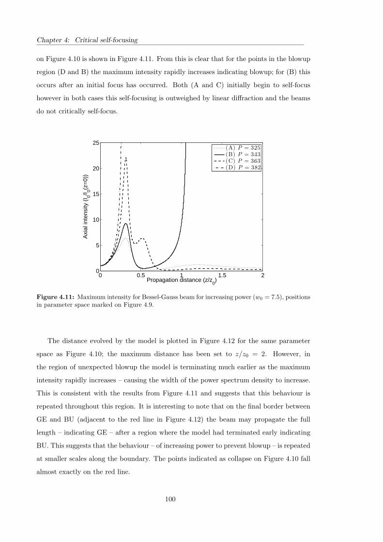
Chapter 4: Critical self-focusing
on Figure 4.10 is shown in Figure 4.11. From this is clear that for the points in the blowup
region (D and B) the maximum intensity rapidly increases indicating blowup; for (B) this
occurs after an initial focus has occurred. Both (A and C) initially begin to self-focus
however in both cases this self-focusing is outweighed by linear diffraction and the beams
do not critically self-focus.
0 0.5 1 1.5 20
5
10
15
20
25
Propagation distance (z/z0)
Axi
al in
tens
ity (
I 0/I 0(z=
0))
(A) P = 3.25(B) P = 3.43(C) P = 3.63(D) P = 3.82
Figure 4.11: Maximum intensity for Bessel-Gauss beam for increasing power (w0 = 7.5), positionsin parameter space marked on Figure 4.9.
The distance evolved by the model is plotted in Figure 4.12 for the same parameter
space as Figure 4.10; the maximum distance has been set to z/z0 = 2. However, in
the region of unexpected blowup the model is terminating much earlier as the maximum
intensity rapidly increases – causing the width of the power spectrum density to increase.
This is consistent with the results from Figure 4.11 and suggests that this behaviour is
repeated throughout this region. It is interesting to note that on the final border between
GE and BU (adjacent to the red line in Figure 4.12) the beam may propagate the full
length – indicating GE – after a region where the model had terminated early indicating
BU. This suggests that the behaviour – of increasing power to prevent blowup – is repeated
at smaller scales along the boundary. The points indicated as collapse on Figure 4.10 fall
almost exactly on the red line.
100

4.7 Conclusions
Figure 4.12: Enlargement from Figure 4.9 showing propagation distance, normalised to z0, beforetermination of the model.
4.7 Conclusions
The fate of initial conditions in the Nonlinear Schrodinger Equation (NSE) may be classi-
fied into one of two sets: blowup (BU) whereby the beam becomes singular within a finite
propagation distance, and global existence (GE) for which the beam remains well defined
(finite) for all space. Furthermore there exists a subset of blowup, collapse (CL), for which
the beam width tends to zero in a finite time.
Using the virial technique, sufficient conditions for GE and CL may be written in terms
of the L2 norm of the initial condition – power in the case of optical beams. When these
conditions are applied to the modified Townes profile it is observed that there are only
regions of GE and CL; there is no region of BU without CL.
When evaluated for a Gaussian beam, these sufficient conditions do not cover the full
parameter space and there is an unknown region, not predicted by sufficient conditions.
In order to evaluate this region the numerical technique HARP is used to model the
101

Chapter 4: Critical self-focusing
evolution of the field. When evaluated numerically, it was shown that there exists a region
for which BU is not accompanied with CL. The boundary between GE and BU is given
by PBU = 1.8958 and is in agreement with previous values obtained for this boundary to
within an accuracy of 0.02%. It is likely that this value is more precise, however as no
exact analytical method exists for determining this value it is only possible to compare
one model against another. This high degree agreement between the value produced by
HARP and previous work by other authors suggests that HARP is highly accurate.
Finally, the Bessel-Gauss profile is considered as an initial condition. Unlike the Gaus-
sian and Townes profiles, the critical powers representing sufficient conditions for the
Bessel-Gauss profile are divergent, resulting in a much larger unknown area which must
be tested numerically.
The numerical results for this region demonstrate that the boundary between GE and
BU increases as the Gaussian envelope is widened. As the Gaussian width is increased the
boundary between GE and BU becomes less well defined, and it is demonstrated that the
Bessel-Gauss beam possesses regions in which increasing the power will cause the beam
fate to move from BU back to GE. Such behaviour is highly counter-intuitive and would
be interesting to investigate if such stabilisation may be observed experimentally.
102

Chapter 5
Zero Order Bessel Beams in
Kerr-like Media
For beam powers below the threshold for critical self-focusing the Bessel-Gauss beam
is known to experience a periodic modulation in intensity in the direction of propagation
[33, 34, 35, 66]. This chapter uses the HARP model developed in Chapter 3 to numerically
investigate this behaviour.
The paraxial results obtained with the HARP model are compared to existing descrip-
tions for the beam behaviour and a deficiency is revealed in the current description of the
modulation length. By relating the propagation behaviour to the beam power the existing
model is adapted to produce a power dependent description for the beat length. This
power dependency is found to accurately describe the modulation length, predicting the
existence of chirp.
Finally the beam is modelled using the difference differential model (Section 3.2.2).
The results are compared to the modified description of modulation length and it is found
that the relation is still accurate for large cone angles and powers surpassing the paraxial
collapse power.
103

Chapter 5: Zero Order Bessel Beams in Kerr-like Media
5.1 The initial Bessel-Gauss beam
The initial beam profile, in normalised co-ordinates, for the zero order Bessel Gauss beam
is given by
u(r, z = 0) = u0J0(rk0r) exp
[−(
r
w0
)2m]
, (5.1)
where k0r is the Bessel transverse frequency, w0 is the 1/e width of the Gaussian window,
u0 is the field scaling, and m is the order of the Gaussian envelope. For m > 1 the envelope
is super-Gaussian, however unless explicitly stated, a value of m = 1 shall be used.
5.1.1 Conversion into real units
The majority of the results presented in this chapter are given in normalised units, intro-
duced in Section 2.3. However, it is important to understand how these normalised units
relate to real quantities. Typically, results in this chapter are presented in terms of central
lobe power, P , Bessel principal frequency, k0r , and Gaussian envelope width, w0. The total
beam power, Pt, is related to P through
Pt =Pk0
rw0
j0,1J1(j0,1)√
(2π)(5.2)
where j0,1 is the first zero of the Bessel function J0. For the values of k0r = 20 and w0 = 5,
that are used in the majority of examples, Pt ' 26P . The total beam power in laboratory
units is given by
P =λ2
n0n22π2Pt (5.3)
where Pt is the total beam power in normalised units. Transverse and longitudinal units
may be rescaled using the relations given in Section 2.3 given
r0 =k0
r
k sin θ, (5.4)
where θ is the inner cone angle in real units.
104

5.2 Preliminary numerical investigation
5.2 Preliminary numerical investigation
Using the paraxial split step method in HARP the propagation of the zero order Bessel-
Gauss beam in a Kerr-like material was modelled. The intensity profile for a slice through
the beam axis is shown in Figure 5.1a for a linear medium, along with the same Bessel-
Gauss profile propagating in a nonlinear medium in Figure 5.1b for comparison. The
dimension of propagation, z has been scaled to the Bessel-Gauss geometric shadow length,
z0 (Section 1.2).
The most obvious difference between the linear and nonlinear propagation is the in-
troduction of periodic intensity modulation in the direction of propagation. The largest
variation in intensity is present in the central lobe, however all of the visible side lobes
experience some degree of modulation.
If it is possible to accurately control this beating behaviour, it may be possible to
use the periodic intensity to locally exceed the threshold for material modification and
generate periodic structures written in materials with a high value of n2.
5.3 Frequency space representation
For beams propagating in a linear medium the transverse power spectrum density does not
vary; however, for a nonlinear medium additional transverse frequencies may be generated
through the nonlinear interactions. Understanding how these additional frequencies arise
yields valuable insight into the overall behaviour of the beam.
Two analytical approaches have been used to investigate the behaviour of the angular
spectrum. In the presence of strong nonlinearity the angular spectrum is evaluated across
a small propagation step in [35], and in the presence of weak nonlinearity the angular
spectrum has been studied by considering the transverse and longitudinal phase matching
requirements in [66]. These approaches are summarised here.
5.3.1 Strong nonlinearity
The behaviour of a beam propagating through a small section of nonlinear space may
be approximated by neglecting the second-order diffraction term in the paraxial wave
equation [35]. This is justified by assuming that the effect of diffraction in negligible
105

Chapter 5: Zero Order Bessel Beams in Kerr-like Media
(a) Linear Bessel-Gauss beam intensity profile.
(b) Nonlinear, paraxial, intensity profile.
Figure 5.1: Comparing results for Bessel-Gauss beams in linear and nonlinear media. In bothcases; k0
r = 20, w0 = 5 and P = 2.
106

5.3 Frequency space representation
over the small step compared to the nonlinearity. In this case the Nonlinear Schrodinger
Equation (NSE) (Equation 2.36) becomes
ddz
u(z) = i|u(z)|2u(z). (5.5)
For a small step δz, this has the approximate solution,
u(z + δz) = u(z) exp(i|u(z)|2δz
). (5.6)
By using Equation 5.1 for the Bessel-Gauss beam Equation 5.6 may be written as
u(r, z + δz) = u0J0(k0rr) exp
[−(
r
w0
)2m]
exp
[i|u0|2δzJ2
0(k0rr) exp[−
(r
w0
)2m
]
]. (5.7)
This may considered as the original field modulated by a exponential phase grating term.
Although only the phase changes in real space, Equation 5.7 may generate additional
angular frequencies since, by analogy with a 1D phase grating, the incoming wave can
diffract off the phase grating into a different direction.
From this, the angular spectrum, |U(z + δz, kr)|2, may be determined by using the
zero order Hankel transform
U(z + δz, kr) = u0
∞∫0
J0(rkr)J0(k0rr) exp
[−(
r
w0
)2m]×
exp
[i|u0|2δzJ2
0(k0rr) exp
[−2(
r
w0
)2m]]
r dr. (5.8)
The power spectral density (PSD) of the angular spectrum depends on the correlation
between the three oscillating terms;
f1 =J0(rkr), (5.9)
f2 =J0(rk0r), (5.10)
f3 =exp
[i|u0|2δzJ2
0(k0rr) exp
[−2(
r
w0
)2m]]
. (5.11)
The maximum contribution from f3 occurs when ∂rJ20(k
0rr) ' 0. Therefore it is ex-
pected that when kr = k0r all three terms are in phase and a maximum is expected in the
107
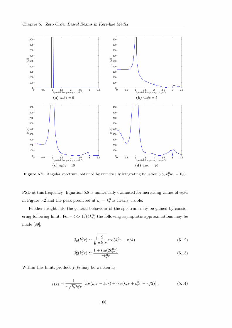
Chapter 5: Zero Order Bessel Beams in Kerr-like Media
0 0.5 1 1.5 2 2.5 3 3.50
100
200
300
400
500
600
700
800
900
|U(k
r)|
Spatial Frequency (kr/k0
r)
(a) u0δz = 0
0 0.5 1 1.5 2 2.5 3 3.50
100
200
300
400
500
600
700
800
900
|U(k
r)|
Spatial Frequency (kr/k0
r)
(b) u0δz = 5
0 0.5 1 1.5 2 2.5 3 3.50
100
200
300
400
500
600
700
800
900
|U(k
r)|
Spatial Frequency (kr/k0
r)
(c) u0δz = 10
0 0.5 1 1.5 2 2.5 3 3.50
100
200
300
400
500
600
700
800
900|U
(kr)|
Spatial Frequency (kr/k0
r)
(d) u0δz = 20
Figure 5.2: Angular spectrum, obtained by numerically integrating Equation 5.8, k0rw0 = 100.
PSD at this frequency. Equation 5.8 is numerically evaluated for increasing values of u0δz
in Figure 5.2 and the peak predicted at kr = k0r is clearly visible.
Further insight into the general behaviour of the spectrum may be gained by consid-
ering following limit. For r >> 1/(4k0r) the following asymptotic approximations may be
made [89];
J0(k0rr) '
√2
πk0rr
cos(k0rr − π/4), (5.12)
J20(k
0rr) '
1 + sin(2k0rr)
πk0rr
. (5.13)
Within this limit, product f1f2 may be written as
f1f2 =1
π√
krk0rr
[cos(krr − k0
rr) + cos(krr + k0rr − π/2)
]. (5.14)
108

5.3 Frequency space representation
When kr = 3k0r the variation of cos(2k0
rr) and the maxima of sin(2k0rr) are correlated,
however the phase shift of π/2 gives rise to the hole in the spectrum visible in Figure
5.2d. For kr < k0r the central lobe from f1 begins to overlap with the second maximum
contribution from f3 leading to the formation of a maximum in the spectrum around
kr = 0.
The presence of an axial field and an outer ring at kr = 3k0r has been verified exper-
imentally [35]. Here the authors formed a Bessel beam by focusing 120ps pulses from a
frequency doubled Nd:YAG laser with a axicon lens. The Bessel beam self-action was
investigated in CdSxSe1−x doped colour glass n2 ' 1.1× 10⁻¹⁹m2/V2 and observed in the
far field to confirm the existence of a split ring at kr = 3k0r .
For weaker nonlinearity the diffraction of the beam dominates and the diffraction term
may no longer be discarded. In this case phase matching arguments may be adopted to
study the beam evolution.
5.3.2 Weak nonlinearity
The behaviour of the Bessel-Gauss beam has also been studied in the presence of weak
nonlinearity through the use of the transverse phase-matching integral [66]. Under the
approximation that diffraction from the Gaussian window is negligible, w0 →∞, a solution
to the paraxial nonlinear wave equation may be written as;
u(r, z) = u0(r) + u1(r, z) + u2(r, z) . . . (5.15)
where uk ∝ nk2.
By expanding Equation 5.15 into the paraxial nonlinear wave equation, and collecting
terms of equal order of n2, a series of nonlinear equations may be obtained. The first two
equations are
∂u1
∂z− i∇2
⊥u1 =i|u0|2u0, (5.16a)
∂u2
∂z− i∇2
⊥u2 =i(2|u0|2u1 + u20u
∗1). (5.16b)
The behaviour from these equations can be thought of as the degenerate four wave
109

Chapter 5: Zero Order Bessel Beams in Kerr-like Media
mixing interaction between the original pump beam, u0 – in this case the initial Bessel-
Gauss beam – and the generated fields, u1 and u2.
Equation 5.16a
Equation 5.16a describes the degenerate interaction between four waves with frequencies
ω4 = ω1−ω2 +ω3; three waves at the pump frequency interact to produce a fourth of the
same frequency. For the wave vector of field n, kn = (knz , kn
r ) in cylindrical co-ordinates.
To conserve momentum, an exact longitudinal phase matching condition requires that
k4z = k1
z − k2z + k3
z and consequently k4r = k1
r = k2r = k3
r = k0r . For the pump frequency
this implies that three waves from the pump cone interact to produces a fourth which is
restricted to the same cone.
The transverse phase matching condition may be given by the transverse phase match-
ing integral (TPMI) which describes the interaction between overlapping conical waves
[90, 91, 92, 93]1. The TPMI for Equation 5.16a is given by
T1(p) =
∞∫0
r exp(−3r2/w2
0
)J30(k
0rr)J0(pr)dr, (5.17)
where p = kr/k0r . Equation 5.17 is evaluated numerically for w0 = 200 and k0
r = 1 in
Figure 5.3. The result of the TPMI is in agreement with the exact longitudinal phase
matching condition; the generated field is strongly phase matched at kr = k0r . This
explains the robust nature of the pump ring in the Bessel-Gauss beam, and leads to the
nonlinear reconstruction for a partially blocked spectrum, whereby a portion of the beam
may be blocked in frequency space. Through the phase matching of Equation 5.16a three
waves from the remaining spectrum may combine to produce a fourth which may lie in
the empty region. Although this bears similarity to the reconstruction of a Bessel beam
that is partially blocked in real space, it should be noted that the underlying principles are
completely different. This reconstruction has been experimentally verified by Sogomonian
et al. [95].
1Further background on the TPMI including derivation may be found in [94]
110
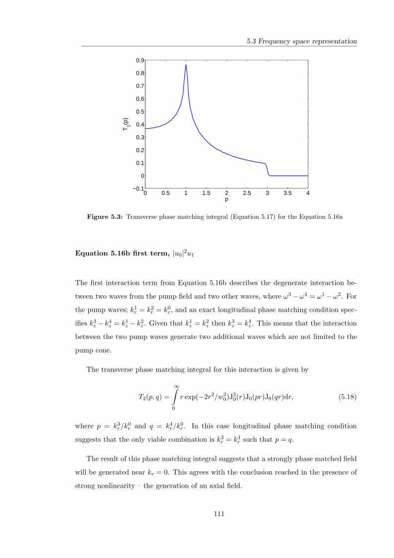
5.3 Frequency space representation
0 0.5 1 1.5 2 2.5 3 3.5 4−0.1
0
0.1
0.2
0.3
0.4
0.5
0.6
0.7
0.8
0.9
p
T1(p
)
Figure 5.3: Transverse phase matching integral (Equation 5.17) for the Equation 5.16a
Equation 5.16b first term, |u0|2u1
The first interaction term from Equation 5.16b describes the degenerate interaction be-
tween two waves from the pump field and two other waves, where ω3−ω4 = ω1−ω2. For
the pump waves; k1r = k2
r = k0r , and an exact longitudinal phase matching condition spec-
ifies k3z − k4
z = k1z − k2
z . Given that k1z = k2
z then k3z = k4
z . This means that the interaction
between the two pump waves generate two additional waves which are not limited to the
pump cone.
The transverse phase matching integral for this interaction is given by
T2(p, q) =
∞∫0
r exp(−2r2/w20)J
20(r)J0(pr)J0(qr)dr, (5.18)
where p = k3r/k0
r and q = k4r/k0
r . In this case longitudinal phase matching condition
suggests that the only viable combination is k3r = k4
r such that p = q.
The result of this phase matching integral suggests that a strongly phase matched field
will be generated near kr = 0. This agrees with the conclusion reached in the presence of
strong nonlinearity – the generation of an axial field.
111

Chapter 5: Zero Order Bessel Beams in Kerr-like Media
0 0.5 1 1.5 2 2.5 30
2
4
6
8
10
12
14
16
18
20
p
T2(p
)
Figure 5.4: Transverse phase matching integral (Equation 5.18) for the second approximationEquation 5.16b
Equation 5.16b second term, u20u
∗1
The term u20u
∗1 is analogous to degenerate parametric amplification [58, 66], in which
case ω3 + ω4 = ω1 + ω2 where ω1 and ω2 lie in the pump cone. This gives an exact
longitudinal phase matching condition of k3z + k4
z = 2k0z and an exact transverse phase
matching condition of k3r + k4
r = 2k0r .
The transverse and longitudinal wavenumbers for the pump cone are related by
(k0r)
2 + (k0z)
2 = k2. (5.19)
The cone angles for the generated fields are given by
k3r =k sin θ3 k4
r = k sin θ4, (5.20)
k3z =k cos θ3 k4
z = k cos θ4. (5.21)
By applying the exact transverse and longitudinal phase matching conditions to Equation
5.19 and then expressing the transverse and longitudinal wavenumbers in terms of the
112

5.3 Frequency space representation
cone angles (Equation 5.20); the following expression is obtained;
(cos θ4 + cos θ3)2
4+
(sin θ4 + sin θ3)2
4= 1. (5.22)
This may be expanded and simplified to yield
cos(θ3 − θ4) = 1. (5.23)
This implies that θ3−θ4 = 0 which will in turn only satisfy the transverse and longitudinal
phase matching conditions in the case that θ3 = θ4 = θ0 and all four waves fall on the
pump cone.
However, it is possible for a field to be generated in the case of a phase mismatch.
Under the small angle approximation the longitudinal phase matching condition may be
written as
θ23 + θ2
4 = 2θ20 (5.24)
and that in turn as
(k3r)
2 + (k4r)
2 = 2(k0r)
2. (5.25)
In the case where an axial field is present such that k3r = 0; the longitudinal phase
matching condition in Equation 5.25 suggests that an additional field may be generated
at k4r =
√2k0
r .
5.3.3 Comparison with numerical examples
The angular spectrum for a Bessel-Gauss beam propagating through a nonlinear medium
is shown in Figure 5.6 for increasing distance in the propagation direction. As the beam
propagates, the axial field predicted by the weak (5.3.2) and strong (Section 5.3.1) non-
linearity is clearly present. Once the axial field has built up the outer ring at kr =√
2k0r
appears as predicted. Although the ring at kr = 3k0r is not visible in Figure 5.6, when
viewed on a logarithmic scale (Figure 5.5) a splitting is present – although at a much
lower power spectral density. This is consistent with the notion that non-phase matched
frequencies are suppressed.
As expected the principal transverse frequency, k0r remains the dominant feature in
the angular spectrum, implying that the beam will retain the Bessel-like transverse peri-
113

Chapter 5: Zero Order Bessel Beams in Kerr-like Media
0 0.5 1 1.5 2 2.5 3 3.510
−10
10−8
10−6
10−4
10−2
100
kr/k0
r
|U|2
Figure 5.5: Figure 5.6d plotted on a log scale.
odic appearance. Initially the bandwidth of the principal frequency component increases;
however, as the beam propagates, spatial frequencies that are not phase matched are sup-
pressed and gradually disappear. This results in the narrowing of the axial component in
frequency space and consequently the broadening of the Gaussian window in real space.
5.4 Low power beat length equation
Both strong and weak nonlinear interactions lead to the generation of an axial field. By
considering this field separately to the Bessel-Gauss beam it is clear that, in real space,
the forward phase evolution will differ; this is summarised in Figure 5.7. The difference
between the axial wave number, k in Figure 5.7, and the z component of the Bessel-Gauss
beam (kz) leads to a phase mismatch, ∆kz. This phase mismatch causes the intensity
modulation observed in Figure 5.1b.
The characteristic length for this modulation behaviour is given by,
z0b =
2π
∆kz, (5.26)
where ∆kz = k − kz. This equation is also obtained by references [33] and [92] and does
not vary with beam power. For this reason Equation 5.26 shall be referred to as the low
114

5.4 Low power beat length equation
0 0.5 1 1.5 2 2.5 3 3.50
0.1
0.2
0.3
0.4
0.5
0.6
0.7
0.8
0.9
1
kr/k0
r
|U|2
(a) z = 0
0 0.5 1 1.5 2 2.5 3 3.50
0.1
0.2
0.3
0.4
0.5
0.6
0.7
0.8
0.9
1
kr/k0
r
|U|2
(b) z = 0.25z0
0 0.5 1 1.5 2 2.5 3 3.50
0.1
0.2
0.3
0.4
0.5
0.6
0.7
0.8
0.9
1
kr/k0
r
|U|2
(c) z = 0.5z0
0 0.5 1 1.5 2 2.5 3 3.50
0.1
0.2
0.3
0.4
0.5
0.6
0.7
0.8
0.9
1
kr/k0
r
|U|2
(d) z = z0
Figure 5.6: Angular spectra for the numerically propagated Bessel-Gauss beam after increasingpropagation lengths. Initial Bessel-Gauss profile; P = 2, w0 = 5 and k0
r = 20. Position of√
2k0r is
indicated as dotted line.
Figure 5.7: Frequency space diagram
115

Chapter 5: Zero Order Bessel Beams in Kerr-like Media
power beat length.
0 1 2 3 4 5 6 70
0.2
0.4
0.6
0.8
1
1.2
1.4
1.6
1.8
2
Propagation distance (z/z0
b)
Norm
ali
sed
axia
lin
tensi
y(I
/I0)
Figure 5.8: Normalised axial intensity, w0 = 5, k0r = 20, P = 2.
Figure 5.8 shows the axial intensity modulation for a Bessel-Gauss beam with w0 = 5,
k0r = 20 and central lobe power P = 2. The distance of propagation, z, has been normalised
to the low power beat length, z0b . From this figure it is clear that, in practice, Equation
5.26 is an overestimate of the beat length. To address this deficiency, the evolution of
the Bessel-Gauss beam is investigated for increasing power, up to the threshold power for
blowup.
5.5 Increasing power
5.5.1 Average intensity and Modulation depth
The average intensity may be defined as the local average about which the intensity is
modulated. For low powers this is equivalent to the linear intensity however as the power
is increased this approximation breaks down.
The depth of modulation is defined as the peak to trough variation in intensity between
successive maxima and minima. By examining Figure 5.8 it is clear that the modulation
116
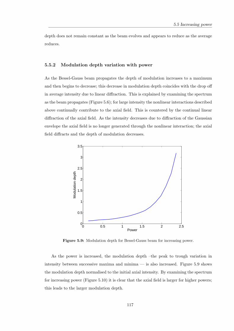
5.5 Increasing power
depth does not remain constant as the beam evolves and appears to reduce as the average
reduces.
5.5.2 Modulation depth variation with power
As the Bessel-Gauss beam propagates the depth of modulation increases to a maximum
and then begins to decrease; this decrease in modulation depth coincides with the drop off
in average intensity due to linear diffraction. This is explained by examining the spectrum
as the beam propagates (Figure 5.6); for large intensity the nonlinear interactions described
above continually contribute to the axial field. This is countered by the continual linear
diffraction of the axial field. As the intensity decreases due to diffraction of the Gaussian
envelope the axial field is no longer generated through the nonlinear interaction; the axial
field diffracts and the depth of modulation decreases.
0 0.5 1 1.5 2 2.50
0.5
1
1.5
2
2.5
3
3.5
Power
Mod
ulat
ion
dept
h
Figure 5.9: Modulation depth for Bessel-Gauss beam for increasing power.
As the power is increased, the modulation depth –the peak to trough variation in
intensity between successive maxima and minima — is also increased. Figure 5.9 shows
the modulation depth normalised to the initial axial intensity. By examining the spectrum
for increasing power (Figure 5.10) it is clear that the axial field is larger for higher powers;
this leads to the larger modulation depth.
117

Chapter 5: Zero Order Bessel Beams in Kerr-like Media
0 0.5 1 1.5 2 2.50
0.005
0.01
0.015
0.02
0.025
0.03
0.035
0.04
0.045
0.05
Tra
nsv
ers
esp
ectr
um
|U(k
r)|
2
Spatial Frequency (kr/k0
r)
(a) P = 0
0 0.5 1 1.5 2 2.50
0.005
0.01
0.015
0.02
0.025
0.03
0.035
0.04
0.045
0.05
Tra
nsv
ers
esp
ectr
um
|U(k
r)|
2
Spatial Frequency (kr/k0
r)
(b) P = 1
0 0.5 1 1.5 2 2.50
0.005
0.01
0.015
0.02
0.025
0.03
0.035
0.04
0.045
0.05
Tra
nsv
ers
esp
ectr
um
|U(k
r)|
2
Spatial Frequency (kr/k0
r)
(c) P = 2
0 0.5 1 1.5 2 2.50
0.005
0.01
0.015
0.02
0.025
0.03
0.035
0.04
0.045
0.05
Tra
nsv
ers
esp
ectr
um
|U(k
r)|
2
Spatial Frequency (kr/k0
r)
(d) P = 2.5
Figure 5.10: Spectrum at z = z0 for increasing power.
5.5.3 Deviation from the beat-length
Figure 5.11 compares three Bessel-Gauss beams with different central lobe powers. In the
low power limit the beam behaves as though it were linear; as the power in the central lobe
is increased the beam becomes modulated in the direction of propagation. Additionally
the beat length appears to reduce for increasing power.
To assess this variation of beat length with power the period is measured using peak
detection (Section 5.6.1) to obtain the characteristic beat length from the axial intensity
data. The variation of beat length obtained in this manner is shown in Figure 5.12, here
the beat length is clearly reduced with increasing power. However the beat length does
appear to converge on Equation 5.26 for low power. As mentioned above the depth of
118

5.5 Increasing power
0 0.2 0.4 0.6 0.8 10
0.2
0.4
0.6
0.8
1
1.2
1.4
1.6
1.8
2
Propagation distance (z/z0)
Norm
ali
sed
axia
lin
tensi
y(I
/I0)
P = 1P = 2Linear
Figure 5.11: Axial intensity for increasing power, w0 = 5, kr = 20.
modulation increases with power; for low power the depth of modulation is very small and
consequently is impossible to accurately determine using a peak detection method. This
leads to a lack of data points as P → 0.
Figure 5.12: Beat length reducing with increasing power.
119

Chapter 5: Zero Order Bessel Beams in Kerr-like Media
5.5.4 Improving the approximation
Two features are not taken into account in the linear approximation. The first deficiency
arises because it has been, incorrectly, assumed that the generated field has the form of a
plane wave, whereas it is Gaussian-like [66]. This accounts for the concentration of power
towards the central lobes.
Furthermore, the Kerr induced phase retardation, on the axial field, has not been taken
into account. As the weak axial field propagates it experiences a higher refractive index
from the Kerr nonlinearity, induced by the Bessel-Gauss beam. This increases the rate at
which the phase evolves in z, effectively increasing the wavenumber by ∆k = kn2/n0I for
the axial field (Figure 5.13). Of course, this effective ∆k will vary due to the intensity
modulation in I. However, an average ∆k may be constructed by considering I as the
averaged intensity over one period of modulation such that ∆k = kn2/n0Ieff where n0
and n2 are the usual linear and nonlinear refractive indices respectively. The effective
intensity may then be written as a modified average intensity; Ieff '< I >. For fixed
beam parameters (k0r and w0) the average intensity will scale linearly with power.
Figure 5.13: Frequency space diagram, increase in effective k indicated as ∆k.
5.5.5 Correcting the beat length
Figure 5.13 shows the increase in effective wavenumber k for the axial field and the con-
tribution this gives to ∆kz. From this, a new nonlinear beat length is proposed, based on
a correction to Equation 5.26 [66];
zb =2π
k(1 + Ieffn2/n0)− kz. (5.27)
120
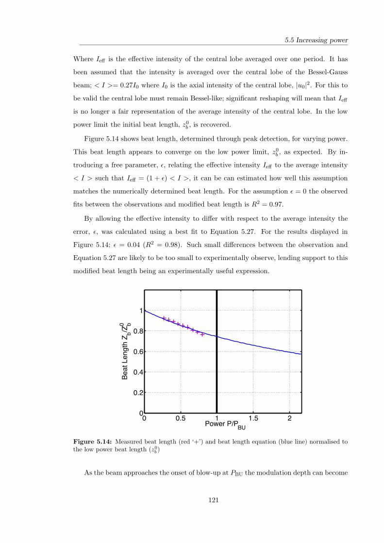
5.5 Increasing power
Where Ieff is the effective intensity of the central lobe averaged over one period. It has
been assumed that the intensity is averaged over the central lobe of the Bessel-Gauss
beam; < I >= 0.27I0 where I0 is the axial intensity of the central lobe, |u0|2. For this to
be valid the central lobe must remain Bessel-like; significant reshaping will mean that Ieff
is no longer a fair representation of the average intensity of the central lobe. In the low
power limit the initial beat length, z0b , is recovered.
Figure 5.14 shows beat length, determined through peak detection, for varying power.
This beat length appears to converge on the low power limit, z0b , as expected. By in-
troducing a free parameter, ε, relating the effective intensity Ieff to the average intensity
< I > such that Ieff = (1 + ε) < I >, it can be can estimated how well this assumption
matches the numerically determined beat length. For the assumption ε = 0 the observed
fits between the observations and modified beat length is R2 = 0.97.
By allowing the effective intensity to differ with respect to the average intensity the
error, ε, was calculated using a best fit to Equation 5.27. For the results displayed in
Figure 5.14; ε = 0.04 (R2 = 0.98). Such small differences between the observation and
Equation 5.27 are likely to be too small to experimentally observe, lending support to this
modified beat length being an experimentally useful expression.
Figure 5.14: Measured beat length (red ‘+’) and beat length equation (blue line) normalised tothe low power beat length (z0
b )
As the beam approaches the onset of blow-up at PBU the modulation depth can become
121

Chapter 5: Zero Order Bessel Beams in Kerr-like Media
extremely large. At this point the assumption that the initial intensity, I0, is a good
approximation for the average intensity over one beat length is less reasonable and a
deviation from Equation 5.27 is observed.
5.5.6 Super Gaussian windows
The propagation of a Bessel-Gauss beam with a super Gaussian window (m > 1 in Equa-
tion 5.1) is broadly similar to the regular Gaussian window. In a linear medium, the
Bessel-super-Gauss beam exhibits a much longer “flat” axial intensity (Section 1.2.3); it is
therefore expected that in a nonlinear medium the average intensity will remain constant
for a similar distance.
Figure 5.15 shows the intensity modulation for a Bessel beam with Gaussian and
super-Gaussian windowing. The propagation length, z, has has been normalised to the
modified beat length zb, which is the same for both beams. The grid markers have been
offset so that the first marker is aligned with the first intensity maxima and the spacing
of subsequent markers is the modified beat-length, zb. It is clear that the Gaussian and
super Gaussian windows initially produce the same beat-length and the maxima coincide
with the grid markers as expected. However, as the average intensity begins to decay the
maxima no longer coincide with the grid markers and the rate at which they diverge is
different between the Gaussian and super-Gaussian windowed beams.
If the intensity modulation were to be used in a process with a threshold-like response
then it may be desirable to have a longer region where the intensity varies around the
same value. As is seen in Figure 5.15 this may be obtained by using a super-Gaussian
window. It has been demonstrated that the axial intensity of a Bessel-like beam in a linear
medium may be precisely engineered [48]. It is possible that a similar technique may be
applied here to provide fine control over the average intensity.
It should be remembered that, as the order of the super Gaussian window is increased
(m >> 1) the windowing of the Bessel beam tends towards truncation by a harsh aperture.
In this limit the intensity oscillates due to linear diffraction (Section 1.2.3). This oscillation
will ultimately reduce the effectiveness of Equation 5.27.
122

5.6 Axial modulation chirp
0 1 2 3 4 5 6 7 8 90
0.2
0.4
0.6
0.8
1
1.2
1.4
1.6
Propagation distance (z/zb)
Norm
ali
sed
axia
lin
tensi
y(I
/I0)
p = 1p = 2p = 1 (Lin)p = 2 (Lin)
Figure 5.15: Comparison of behaviour for Gaussian and super-Gaussian windows, w0 = 5,k0
r = 20.
5.6 Axial modulation chirp
If this modulation behaviour is to be used to write periodic structures in materials with
high n2 then it is important that either the beat length does not vary across the periods
or if the beat length does vary it is important to understand the cause and potentially
manipulate any variation, or chirp when it is desired.
By inspecting Figure 5.16 it is apparent that, for the first four maxima the modified
beat length provides a good description of the axial modulation length. As the intensity
decays then the observed beat length in Figure 5.16 increases, departing from Equation
5.27. This suggests that there may exist a chirp in the intensity modulation which acts as
a function of intensity.
5.6.1 Accurately measuring the beat-length
In order to address the apparent chirp in Figure 5.16 a method is required to accurately
measure the beat length. Three methods for assessing the beat length – peak detection,
Fourier representation and the continuous wavelet transform – are briefly discussed here.
123

Chapter 5: Zero Order Bessel Beams in Kerr-like Media
0 1 2 3 4 5 6 7 8 90
0.2
0.4
0.6
0.8
1
1.2
1.4
1.6
1.8
2
Propagation distance (z/zb)
Norm
ali
sed
axia
lin
tensi
y(I
/I0)
P = 2P = 1.5P = 1Linear
Figure 5.16: Normalised axial intensity for increasing powers, w0 = 5, k0r = 20, and Gaussian
window.
Peak detection
The beat length may be crudely determined by measuring the distance between successive
maxima or minima. Naively the position of these maxima and minima may be determined
by using a zero derivative method; however, this is prone to error in the presence of even
small amounts of noise. Peak detection is the name given to a method in which the local
maxima are located for a signal in the presence of small amount of noise.
By locating the maximum for each period a measure of the beat length may be made.
For the results described above, peak detection has been used to calculate the beat length
by averaging over several periods. The method is simple but prone to small amounts of
error.
The first maximum of axial intensity modulation is shown in Figure 5.17, a higher
frequency variation is clearly visible. This higher frequency may cause the local maxima
to shift leading to an error in the beat length. Averaging over several periods reduces the
effect of this error at the expense of accuracy in the position.
A further problem with the peak detection method is that the beat length can only be
measured discretely between maxima and minima. Ideally it is desirable to understand
how the beat length may vary in less coarse steps.
124

5.6 Axial modulation chirp
0 0.01 0.02 0.03 0.04 0.05 0.061
1.1
1.2
1.3
1.4
1.5
1.6
Propagation distance (z/z0)
Norm
ali
sed
axia
lin
tensi
y(I
/I0)
Figure 5.17: Normalised axial intensity for first beat period. Maximum marked as ‘x’, notice thehigh frequency ripples present.
Fourier representation
The most obvious of choices for assessing the frequency components from a signal is the
fast Fourier transform. When the signal is well defined in the space-bandwidth sense
(Section 3.3) then the Fourier spectrum, evaluated using the FFT, completely defines the
real space signal. This does not necessarily mean that the data is represented in a form
from which the signal chirp may be easily determined.
The FFT for the axial intensity in Figure 5.16 is shown in Figure 5.18. To reduce
aliasing artifacts, the intensity has been mirrored about z = 0. The spatial frequency
has been normalised relative to the ∆kz (Section 5.5.5). The large peak near kz = 0
corresponds to the linear drop-off of the axial intensity. As expected the principal beating
frequency, near kz = ±∆kz, is clearly visible. The width of the peak suggests that there
are multiple frequencies contributing to the intensity modulation, possibly indicating the
existence of chirp. However, it is impossible to tell from Figure 5.18 how the chirp varies
in z.
125

Chapter 5: Zero Order Bessel Beams in Kerr-like Media
−2 −1 0 1 20
0.005
0.01
0.015
0.02
0.025
0.03
0.035
0.04
0.045
0.05
Spatial Frequency (kz/∆kz)
Axia
lin
tensi
tyP
SD
(|U
(kz)|
2)
Figure 5.18: Fast Fourier transform of intensity modulation
Continuous wavelet transform
Another option for assessing the chirped beat-length is the continuous wavelet transform
[96]. Unlike the Fourier transform, the CWT may be used to calculate a spectral repre-
sentation of a signal as a function of position in that signal.
Figure 5.19: Scalogram of the axial intensity in Figure 5.16.
126

5.7 Analysis of chirp
The complex Morlet wave-packet was used with the CWT to analyse the axial intensity
modulation. The resulting scalogram is displayed in Figure 5.19. Here the CWT was re-
normalised relative to the maximum intensity at each point in z. This reveals a ridge
that represents the strongest frequency at each position in z (this ridge is highlighted by
the white line in Figure 5.19). Since the Morlet wavelet is a proxy for frequency [96], the
CWT scalograms may be re-scaled so that the period is given. This is more convenient
when comparing to the beat length equations discussed above. Care must be taken when
using the CWT for this kind of analysis because edge effects may distort the ridge; this is
apparent in Figure 5.19 towards the end of propagation. The same is true for the higher
periods displayed for low values of z, although in this case they do not change the location
of the ridge.
5.7 Analysis of chirp
The ridge in the scalogram for the axial modulation intensity (Figure 5.19) suggests that
the beat-length is indeed chirped as a casual observation of Figure 5.16 would suggest.
So far it has been assumed that the intensity-dependent term in Equation 5.27 depends
only on the initial intensity and this has provided a reasonable description of the beat
length for the first few periods. However, after this the signal becomes noticeably chirped.
This may be explained by considering the decay in intensity due to the linear diffraction of
the beam. As the linear Bessel-Gauss beam propagates, the intensity drops off smoothly
(Section 1.2.3). Using this linear intensity in Equation 5.27 instead of the initial intensity
suggests that the beat length will increase as the beam propagates. This agrees with the
observations made from Figure 5.19.
By using the intensity behaviour from a linear model, an estimate for the chirped beat
length may be determined by re-writing Equation 5.27 as
zb(z) =2π
k(1 + Ilin(z)n2/n0)− kz, (5.28)
where Ilin(z) is the effective intensity as a function of z, obtained from a linear description
of the beam evolution. Equation 5.28 is plotted in Figure 5.19 as the black line and is
clearly a very good description of the chirped beat length.
127
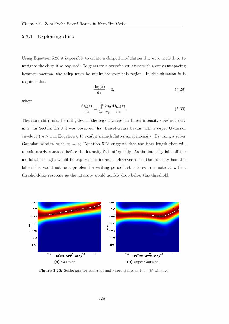
Chapter 5: Zero Order Bessel Beams in Kerr-like Media
5.7.1 Exploiting chirp
Using Equation 5.28 it is possible to create a chirped modulation if it were needed, or to
mitigate the chirp if so required. To generate a periodic structure with a constant spacing
between maxima, the chirp must be minimised over this region. In this situation it is
required thatdzb(z)
dz= 0, (5.29)
wheredzb(z)
dz=
z2b
2π
kn2
n0
dIlin(z)dz
. (5.30)
Therefore chirp may be mitigated in the region where the linear intensity does not vary
in z. In Section 1.2.3 it was observed that Bessel-Gauss beams with a super Gaussian
envelope (m > 1 in Equation 5.1) exhibit a much flatter axial intensity. By using a super
Gaussian window with m = 4; Equation 5.28 suggests that the beat length that will
remain nearly constant before the intensity falls off quickly. As the intensity falls off the
modulation length would be expected to increase. However, since the intensity has also
fallen this would not be a problem for writing periodic structures in a material with a
threshold-like response as the intensity would quickly drop below this threshold.
(a) Gaussian (b) Super Gaussian
Figure 5.20: Scalogram for Gaussian and Super-Gaussian (m = 8) window.
128

5.8 Propagation through full focus
5.8 Propagation through full focus
All of the Bessel-Gauss beams modelled so far have been propagated from the nominal
focus of the beam (Figure 5.21), insomuch as they have all had a flat phase front. This
is equivalent to positioning the Bessel-Gauss beam so that the focus lies on the surface of
the nonlinear material. If this technique were to be used to write periodic structures in a
nonlinear material then this kind of structure would only be possible next to the surface of
the material. If, however, the beam is modelled from a position before the nominal focus
then it is possible to assess the feasibility of writing periodic structures further within the
nonlinear material.
This section deals with the propagation of Bessel-Gauss beams through the nominal
focus shown in Figure 5.21.
Figure 5.21: Overlap region for Bessel-Gauss beam.
To model the propagation through full focus a Bessel-Gauss is propagated backwards
using a linear model to z = −z0. This field is then used as the initial condition in the
HARP model to propagate the beam forwards a distance of 2z0.
5.8.1 Beam blowup
Figure 5.22 shows the axial intensity for the Bessel-Gauss beam propagated through full
focus as well as the same beam propagated from the nominal focal point. Both beams have
identical initial conditions prior to the linear back propagation. For the beam propagated
129

Chapter 5: Zero Order Bessel Beams in Kerr-like Media
−1 −0.5 0 0.5 10
0.2
0.4
0.6
0.8
1
1.2
1.4
1.6
1.8
2
Propagation distance (z/z0)
Norm
ali
sed
axia
lin
tensi
y(I
/I0)
(a)
0 0.1 0.2 0.3 0.41
1.02
1.04
1.06
1.08
1.1
1.12
1.14
1.16
1.18
1.2
Propagation distance (z/z0)
Norm
ali
sed
axia
lin
tensi
y(I
/I0)
(b) Enlarged section from Figure 5.22a
Figure 5.22: Axial intensity for a Bessel-Gauss beams propagating through full focus (solid) andfrom the nominal focus (dashed) in a nonlinear medium w0 = 5,k0
r = 20,P = 2.
from the nominal focus, the usual intensity modulation is observed. However when the
beam is propagated through the full focus the modulation depth is considerably smaller.
Figure 5.22b shows a zoomed in region from Figure 5.22a showing the much smaller inten-
sity modulation. As is the case when the beam is propagated from the nominal focus, the
beam propagated through full focus experiences a larger amplitude of intensity modula-
tion as the beam power is increased. However, the beam power in Figure 5.22a is already
close to the blow-up threshold. Despite this, the power of beam propagated through full
focus may be increased far beyond this threshold before blow-up is observed. For the
beam propagated through full focus from z = −z0 blowup occurs at P ' 1.8PBU, where
PBU is the blowup power of the same Bessel-Gauss beam propagated from z = 0. As was
observed in Chapter 4 the precise dynamics of blow-up are extremely complicated and
the study of blowup in the case of propagation through full focus would be the subject of
further work.
5.8.2 Intensity modulation
Figure 5.23 shows the axial intensity for a Bessel-Gauss beam propagated through the full
focus, with sufficient power that the intensity modulation is clearly visible. Initially there
is no observable intensity modulation, the intensity of the beam is too small and the beam
behaves as if it were linear. As the intensity increases the nonlinear interaction induces
130

5.8 Propagation through full focus
−1 −0.5 0 0.5 10
0.2
0.4
0.6
0.8
1
1.2
Propagation distance (z/z0)
Norm
ali
sed
axia
lin
tensi
y(I
/I0)
Figure 5.23: Axial intensity for a high-power Bessel-Gauss beam propagating through full focusin a nonlinear medium, w0 = 5,k0
r = 20,P = 3.
an axial field in a similar manner to the beam propagated from the nominal focus. This
leads to the build-up of an axial intensity modulation.
5.8.3 Modulation length
As previously observed, the chirp present in the intensity modulation acts as a function of
linear intensity. Therefore it is reasonable to expect the period of intensity modulation of a
beam propagating through full focus to initially begin to decrease and then increase again
as the intensity drops off. This is not easy to verify numerically; the modulation depth is
initially too small to measure, with either the peak detection or CWT, and indeed when
the intensity is low enough that the beam may be considered linear there is no intensity
modulation to measure.
The CWT of the axial intensity from Figure 5.23 is shown in Figure 5.24. Initially
there is no detectable beat length; however, once the intensity begins to increase, the
beat length behaves as predicted. The spread out area in Figure 5.24 represents local
uncertainty about the period of the beam.
The predicted beat length – from Equation 5.28 – is shown in figure Figure 5.24. In
131

Chapter 5: Zero Order Bessel Beams in Kerr-like Media
Figure 5.24: Scalogram for full focus
this case the beat length is less accurate than the beam propagated from the nominal
focus (Section 5.7). When the axial intensity in Figure 5.23 is compared to the linear case
it is clear that the average intensity for propagation through full focus has been increased.
This is in contrast to the beam propagated from the nominal focus where the average
intensity does not differ much from the linear case.
To take this difference in intensity into account a self-focusing factor α is incorporated
into Equation 5.28. This represents the difference between the linear intensity and the
envelope intensity for the beam propagated through full focus. This value is simply de-
termined by comparing the relative intensities in Figure 5.23. The chirped beat-length
equation may now be written as,
zb =2π
k(1 + αIlin(Z)n2/n0)− kz, (5.31)
where α = 1.2 for Figure 5.23.
Figure 5.25 shows the corrected beat length compared to the chirp obtained from the
scalogram. This is in much better agreement with the beat-length determined from the
CWT. The difference in the region prior to the nominal focus suggests that the difference
between the linear intensity and envelope intensity is due to self-focusing of the central
lobe. Once the nonlinear self-focusing has re-shaped the central lobe the chirped beat
length is in agreement with Equation 5.31.
132

5.9 Seeding with a Gaussian
Figure 5.25: Improved equation for the chirped beat-length (Equation 5.31) α = 1.2.
5.8.4 Further work
A further study into the precise dynamics of self-focusing in this situation is beyond the
scope of this work. Further work would look into the behaviour of the blow-up and collapse
boundaries for Bessel-Gauss beams propagating through full focus. Additionally the exact
nature of the self-focusing of the central lobe is not properly explored here, although the
simple modification to Equation 5.28 to yield Equation 5.31 proves effective in predicting
the chirped beat-length it is not a practical solution to require a full nonlinear model,
effectively defeating the point in Equation 5.31. Potentially a moving focus model may be
applied to the problem to obtain a better estimate for the envelope intensity without the
need to run a whole nonlinear simulation for the problem.
5.9 Seeding with a Gaussian
The axial modulation of the Bessel-Gauss beam is attributed to the interference between
the Bessel-Gauss beam and axial beam generated through the nonlinear interaction (Sec-
tion 5.4). By “seeding” this field it may be possible to adjust the position of the maxima
and minima of the intensity modulation. This would be achieved by using a Gaussian
beam as the seed and then varying the absolute phase of this seed beam.
133

Chapter 5: Zero Order Bessel Beams in Kerr-like Media
The initial condition for this seeded beam is the superposition
u(z = 0, r) = ug(r) exp(iφ) + ub(r), (5.32)
where ub and ug are the Bessel-Gauss beam and Gaussian seed respectively. These are
given by
ub =u0b exp(−r2/w2
0)J0(k0rr), ug =u0
g exp(−r2/w21), (5.33)
where w1 is the width of the Gaussian seed, u1 is the relative weighting and φ is the phase
offset. In the absence of nonlinearity this combination produces a similar beating behaviour
observed for Bessel-Gauss in the presence of nonlinearity (Figure 5.26). However, if the
Gaussian seed is narrow compared to the Gaussian envelope, the behaviour is short-lived
due to the short diffraction length of the Gaussian seed.
0 0.2 0.4 0.6 0.8 10
0.5
1
1.5
Propagation distance (z/z0)
Norm
ali
sed
axia
lin
tensi
y(I
/I
b)
0π
Figure 5.26: Axial intensity for a seeded Bessel-Gauss beam propagating in the absence ofnonlinearity.
Including the Gaussian seed considerably increases the complexity of the initial con-
dition. There are now six parameters (w0,k0r ,u
0b ,φ,w1 and u0
g) which may be varied inde-
pendently. To simplify the situation, suitable parameter are sought given the criteria that
134

5.9 Seeding with a Gaussian
they must not cause the beam to blow-up for any value of φ ∈ [0, 2π].
5.9.1 Beam blow-up
It is important to remember that the power contribution from the seed beam must not
significantly increase the beam power for any value of φ otherwise the beam may enter a
region of blow-up or collapse. Therefore a seed width of w1 << w0 is selected combined
with a relative weighting of u0g < u0
b .
The whole beam power for Equation 5.32 may be given by
P (z = 0) =2π
∞∫0
|u(z = 0, r)|2rdr (5.34)
=Pb + Pg + Pbg, (5.35)
where Pb and Pg are the powers of the Bessel-Gauss beam and the Gaussian seed respec-
tively; and Pbg is the power from the interference. These separate powers may be written
as;
Pg =2π
∞∫0
| exp(iφ)ug(r)|2rdr
=14(u0
g)2w2
1 (5.36)
Pb =2π
∞∫0
|ub(r)|2rdr
=14(u0
b)2w2
0 exp[−1
4(k0
r)2w2
0
]I0
(14(k0
r)2w2
0
)(5.37)
Pbg = + 4π cos(φ)
∞∫0
ug(r)ub(r)rdr
+cos φu0
bu0g
1w2
0+ 1
w21
exp
[(k0
r)2
1w2
0+ 1
w21
]. (5.38)
Given that (k0r)
2w20 >> 1 Equation 5.37 may be written as
Pb '1√4π
w0
k0r
(1 +
12w2
0(k0r)2
), (5.39)
135

Chapter 5: Zero Order Bessel Beams in Kerr-like Media
and if w1 << w0 Equation 5.38 may be written as
Pbg ' 4π cos(φ)u0bu
0gw
21 exp
[−1
4(k0
r)2w2
1
]. (5.40)
Therefore, in the same limits that w1 << w0 and (k0r)
2w20 >> 1 the dominant term in
Equation 5.34 will be Pb – the power of the initial Bessel-Gauss beam – implying that
the overall power will not change significantly. This, however does not exclude blow-up or
collapse, since the blow-up and collapse boundaries are highly sensitive to the initial field,
and indeed the condition for blow-up may be only determined numerically (Section 4.3).
5.9.2 Numerical results
The axial intensities in Figure 5.27 were obtained by selecting values of w0,k0r and u0
b that
would leave the beam power well below the threshold for blow-up – w0 = 5, k0r = 20,
PL = 2. The width of the Gaussian seed was kept small, w1 = 3/k0r = 0.15 and the
relative weighting, u0g, was varied as a percentage of u0
b . Finally, for each value of u0g the
phase is varied between 0 and π.
Even for small seeds – u0g = 0.1u0
b in Figure 5.27a – the position of the maxima may be
moved until they are entirely out of phase. It is interesting to note that when the seed is out
of phase with the Bessel-Gauss beam the amplitude of the intensity modulation is greatly
reduced, for Figure 5.27a this is 20% of the amplitude when the seed is in phase with the
Bessel-Gauss beam. Although the global power does not vary significantly – in this case
P (φ = π) = 99.5%P (φ = 0) – the local power in the central lobe has been changed. It is
suggested that the local power in the central lobe is responsible for modulation depth.
As the seed weighting is increased the increase in local power causes the depth of
modulation to become much larger. Eventually the average intensity increases such that
the beat length, when the seed is in phase with the Bessel-Gauss beam, is noticeably
reduced. This is visible in Figure 5.27d.
Figure 5.28 compares the case of φ = 0, π from Figure 5.27b (u0g = .2u0
b). Although
the amplitude of intensity modulation is much larger for φ = 0 the beat length has been
moved almost exactly out of phase.
To assess the beat length for the seeded beams, the CWT scalograms for the intensities
in Figure 5.28 are shown in Figure 5.29. Again the ridge is plotted in white and the black
136
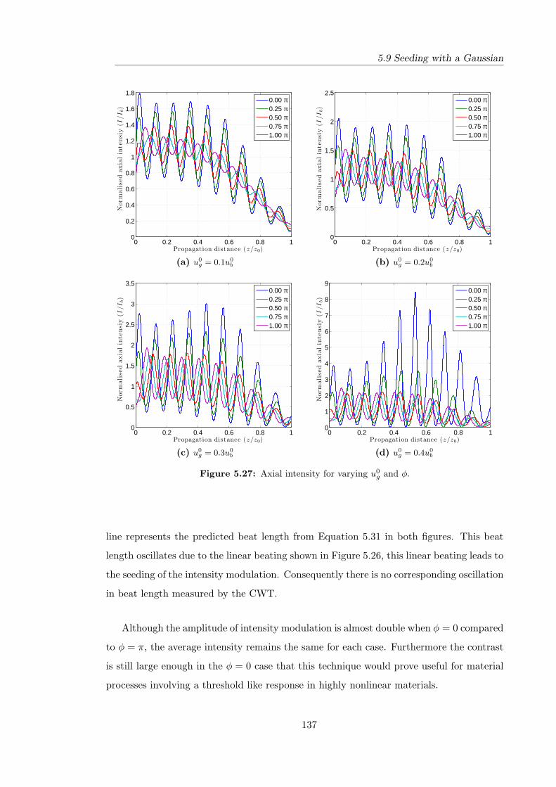
5.9 Seeding with a Gaussian
0 0.2 0.4 0.6 0.8 10
0.2
0.4
0.6
0.8
1
1.2
1.4
1.6
1.8
Propagation distance (z/z0)
Norm
ali
sed
axia
lin
tensi
y(I
/I
b)
0.00 π0.25 π0.50 π0.75 π1.00 π
(a) u0g = 0.1u0
b
0 0.2 0.4 0.6 0.8 10
0.5
1
1.5
2
2.5
Propagation distance (z/z0)
Norm
ali
sed
axia
lin
tensi
y(I
/I
b)
0.00 π0.25 π0.50 π0.75 π1.00 π
(b) u0g = 0.2u0
b
0 0.2 0.4 0.6 0.8 10
0.5
1
1.5
2
2.5
3
3.5
Propagation distance (z/z0)
Norm
ali
sed
axia
lin
tensi
y(I
/I
b)
0.00 π0.25 π0.50 π0.75 π1.00 π
(c) u0g = 0.3u0
b
0 0.2 0.4 0.6 0.8 10
1
2
3
4
5
6
7
8
9
Propagation distance (z/z0)
Norm
ali
sed
axia
lin
tensi
y(I
/I
b)
0.00 π0.25 π0.50 π0.75 π1.00 π
(d) u0g = 0.4u0
b
Figure 5.27: Axial intensity for varying u0g and φ.
line represents the predicted beat length from Equation 5.31 in both figures. This beat
length oscillates due to the linear beating shown in Figure 5.26, this linear beating leads to
the seeding of the intensity modulation. Consequently there is no corresponding oscillation
in beat length measured by the CWT.
Although the amplitude of intensity modulation is almost double when φ = 0 compared
to φ = π, the average intensity remains the same for each case. Furthermore the contrast
is still large enough in the φ = 0 case that this technique would prove useful for material
processes involving a threshold like response in highly nonlinear materials.
137

Chapter 5: Zero Order Bessel Beams in Kerr-like Media
0 0.2 0.4 0.6 0.8 10
0.5
1
1.5
2
2.5
z/z0
u 0(z)/
u 0(z=
0)
φ = 0φ = π
Figure 5.28: Axial intensity for seeded beam for φ = 0 and φ = π.
(a) φ = 0 (b) φ = π
Figure 5.29: Scalogram for seeded Bessel-Gauss beams.
5.10 Seeding through full focus
Although the intensity modulation through full focus has been demonstrated to behave
as predicted in Section 5.8.2, for the purpose of writing structures, it is more suitable to
have considerably more contrast – between the peaks and troughs – and a more consistent
modulation depth through the whole nominal focus. To achieve these aims the seeding
technique may be applied to the full focal propagation on the beam.
The axial intensity for a seeded Bessel-Gauss beam propagating through full focus is
displayed in Figure 5.31. In this case the linear focus of the Gaussian seed beam lies at
138
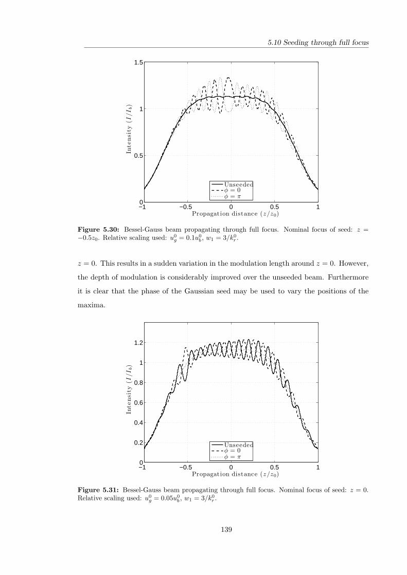
5.10 Seeding through full focus
−1 −0.5 0 0.5 10
0.5
1
1.5
Propagation distance (z/z0)
Inte
nsi
ty(I
/I
b)
Unseededφ = 0φ = π
Figure 5.30: Bessel-Gauss beam propagating through full focus. Nominal focus of seed: z =−0.5z0. Relative scaling used: u0
g = 0.1u0b , w1 = 3/k0
r .
z = 0. This results in a sudden variation in the modulation length around z = 0. However,
the depth of modulation is considerably improved over the unseeded beam. Furthermore
it is clear that the phase of the Gaussian seed may be used to vary the positions of the
maxima.
−1 −0.5 0 0.5 10
0.2
0.4
0.6
0.8
1
1.2
Propagation distance (z/z0)
Inte
nsi
ty(I
/I
b)
Unseededφ = 0φ = π
Figure 5.31: Bessel-Gauss beam propagating through full focus. Nominal focus of seed: z = 0.Relative scaling used: u0
g = 0.05u0b , w1 = 3/k0
r .
139

Chapter 5: Zero Order Bessel Beams in Kerr-like Media
In order to remove this inconsistency in the modulation length, the focus of the Gaus-
sian seed may be moved away from the focus of the Bessel-Gauss beam. In Figure 5.30
the focus of the Gaussian seed lies at z = −0.5z0. By doing this the beat length remains
much more consistent through the focal region and again the phase of the Gaussian beam
may be used to fine tune the positions of the maxima.
5.11 Nonparaxial Beams
To model the behaviour of nonparaxial Bessel-Gauss beams in a nonlinear medium the dif-
ference differential method – Section 2.6.2 – is used as the propagation step in HARP. This
model is a hybrid finite difference method based on the nonparaxial nonlinear Schrodinger
equation (NNSE);
κ∂2u
∂z2+ i
∂u
∂z+∇2
⊥u + |u|2u = 0 (5.41)
Critically the inclusion of the second-order term in z also requires the inclusion of the
constant κ. This constant places a fixed relation between the scaled length in the model
and the wavelength. Unlike the paraxial case where a set of results would be true for any
cone angle; the results obtained from the nonparaxial model is only valid for a specific
cone angle;
θ = sin−1(√
2κk0r
)(5.42)
5.11.1 Resilience to collapse
The inclusion of the second-order diffraction term in z in Equation 5.41 has been demon-
strated to stave off critical self-focusing and in some cases it has been shown to prevent it
entirely. Although the difference differential method does not provide a definitive answer;
for a restricted range of cone angles it is possible to demonstrate that the nonparax-
ial Bessel-Gauss beam may exist for powers surpassing the paraxial threshold power for
blowup.
A shallow cone angle, θ, implies a smaller value of κ. The modelling of high power
beams in this condition becomes extremely computationally demanding. For large cone
angles, θ > 40◦, too much power is truncated in the frequency space boundary and the
model cannot be relied upon to produce reliable results. For sufficiently large values of κ
both the truncated spatial frequencies and the backward propagation must be taken into
140

5.11 Nonparaxial Beams
account.
0 2 4 6 80
0.2
0.4
0.6
0.8
1
1.2
1.4
1.6
1.8
2
Propagation distance (z/z0
b)
Norm
ali
sed
axia
lin
tensi
y(I
/I0)
Figure 5.32: Axial intensity for nonparaxial Bessel-Gauss beam; θ = 35, k0r = 20, w0 = 5, P = 4
(1.5Pc).
The axial intensity for a Bessel Gauss beam well above the paraxial threshold for
blowup is shown in Figure 5.32. The behaviour is largely similar to the sub-critical power
for both paraxial and nonparaxial beams.
5.11.2 Beat length equation
The axial intensities for nonparaxial Bessel-Gauss beams of increasing cone angle are shown
in Figure 5.33. It is assumed that the nonlinear behaviour of the nonparaxial Bessel-Gauss
beam is broadly similar to the paraxial beam. The nonlinear interaction still generates an
axial field which evolves at a different rate to the Bessel-Gauss beam in turn leading to
the familiar intensity modulation.
As the cone angle is increased, for the same power, the amplitude of intensity modula-
tion is visibly reduced. This is attributed to the rate at which the axial field diffracts. A
Bessel-Gauss beam formed from a large cone angle will have a much smaller central lobe
width. Since it is assumed that the generated field is quasi-Gaussian and of size compara-
ble to the central lobe then it is implied that for a larger cone angle the axial field will have
141

Chapter 5: Zero Order Bessel Beams in Kerr-like Media
a much shorter Rayleigh length. Since the beams in Figure 5.33 all posses equal power
– both globally and in the central lobe – the rate at which the axial field is generated
through the nonlinear interaction will remain approximately the same. This combined
with the faster diffraction for large cone angles leads to a reduction in the amplitude of
intensity modulation for increasing cone angle.
0 2 4 6 80
0.2
0.4
0.6
0.8
1
1.2
1.4
1.6
1.8
2
Propagation distance (z/z0
b)
Norm
ali
sed
axia
lin
tensi
y(I
/I0)
10◦20◦30◦40◦
Figure 5.33: Axial intensity for nonparaxial Bessel-Gauss beams for increasing inner cone angles;k0
r = 20, w0 = 5, P = 2.
For the nonparaxial beam, the beat length is still described by the modified beat-
length Equation 5.27, however the longitudinal wavenumber kz must be expressed in the
nonparaxial regime;
kz =√
k2 − (k0r)2. (5.43)
The beat length, determined through peak detection, for increasing power plotted in
Figure 5.34. As with the paraxial results, the modified beat length equation (Equation
5.27 provides a good description of the beat length for increasing power. Furthermore the
beat length equation remains accurate for powers surpassing the paraxial critical power
for blowup. For the points plotted in Figure 5.34 R2 = 0.95. If the fitting parameter ε
is introduced (Section 5.5.5) such that Ieff = (1 + ε) < I > then a best fit is found when
ε = 0.05 (R2 = 0.96).
142
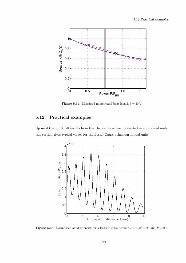
5.12 Practical examples
Figure 5.34: Measured nonparaxial beat length θ = 30◦.
5.12 Practical examples
Up until this point, all results from this chapter have been presented in normalised units,
this section gives typical values for the Bessel-Gauss behaviour in real units.
0 2 4 6 8 100
0.5
1
1.5
2
2.5
3
3.5
4x 10
11
Propagation distance (mm)
Axia
lin
tensi
ty(W
/cm
2)
Figure 5.35: Normalised axial intensity for a Bessel-Gauss beam, w0 = 5, k0r = 20 and P = 2.5
143

Chapter 5: Zero Order Bessel Beams in Kerr-like Media
As an example the axial intensity modulation given in Figure 5.35 is considered. The
parameters for the initial Bessel-Gauss beam in normalised units are, w0 = 5, k0r = 20 and
P = 2.5 – where P is the power in the central lobe – this results in a maximum initial
intensity or I0 = 150.
Although little is known about the exact material parameters for HMO glass it is as-
sumed that a wavelength of approximately 800nm would be suitable for writing structures.
The additional material parameters, n0 = 2.238 and n2 = 5× 10⁻¹⁹m2/Ware taken from
[1].
A power of P = 2.5 in the central lobe corresponds to a total power of Pt ' 64. Using
Equation 5.3 and the material parameters given above gives a total beam power of 2MW
and a central lobe power of 0.08MW. These powers are comparable to the beam powers
used in [38].
By writing Equation 5.7 in terms of wavelength, the low power beat length equation
may be expressed as
z0b =
λ
1− cos θ. (5.44)
From this it is clear that the modulation length will always be larger that the wavelength.
As an example a paraxial Bessel beam formed with an inner cone angle of θ = 2◦ – corre-
sponding to a central spot size of 10µm– results in a low power beat length of z0b = 1mm,
a geometric shadow length, z0 = 12mm and initial intensity on axis is 1.5 × 10¹¹W/cm2.
This, relatively large, beat length is not very useful for the practical generation of periodic
structures. However, a more nonparaxial beam of θ = 40◦ results in a beat length of
3.4µm, and is within the range of wavelengths transparent in HMO glass.
For this beam, the periodic modulation causes the axial intensity to exceed 200% of
the initial value. This suggests that a similar beam may be used to periodically exceed
the threshold for local material modification through multiphoton ionisation.
5.13 Conclusions
As a Bessel-Gauss beam propagates through a nonlinear material the intensity is periodi-
cally modulated in the direction of propagation. It is suggested that, subject to adequate
control over the nature of this modulation, this may be applied as a method for the
construction of periodic structures in materials with high nonlinear refractive indices.
144
5.13 Conclusions
Crucially the period of the intensity modulation must be predictable. Naively the
period may be controlled by adjusting the Bessel principal frequency, k0r , in Equation
5.26. However, this beat-length equation does not accurately describe the behaviour as
the beam power is increased. To address this, a modification to this equation is suggested
in Equation 5.27, providing a greatly improved description of the beam behaviour.
As the beam propagates the beat length becomes noticeably chirped. Neither the pres-
ence nor absence of chirp in the beat length is an explicit prerequisite for the construction
of periodic structures. However, understanding the origin of this chirp may allow further
control. By inserting the linear envelope intensity into the improved beat length equation
a prediction of the chirp on the intensity modulation may be made. This prediction is in
agreement with the measurements taken from numerical simulations. Once it is under-
stood that the chirp may be controlled by adjusting the linear intensity it is possible to
selectively enhance or eliminate chirp as required.
When propagated through full focus the beam exhibits the same periodic modulation,
however the amplitude of modulation is considerably reduced. Furthermore the envelope
intensity has been reshaped. The beat length may be correctly predicted provided the
intensity is corrected to account for this reshaping.
145

Chapter 5: Zero Order Bessel Beams in Kerr-like Media
146
Chapter 6
Nonlinear Bessel Beams
The concept of a stationary solution was introduced in Section 1.2 and the Bessel beam
was shown to exist as a stationary solution to the linear wave equation. Furthermore,
the idea of stationary solutions to the nonlinear wave equation was introduced in Section
4.1.3 with reference to the Townes profile. However there also exists a set of stationary
solutions to the NSE for positive eigenvalues. These solutions are known as nonlinear
Bessel functions due to the shared characteristics with the linear Bessel function. Like the
linear counterpart the nonlinear Bessel beam carries infinite power and is therefore not
physically realistic, however the truncated beam may be shown to be pseudo-stationary.
The propagation of truncated nonlinear Bessel beams is compared to the propagation of
linear Bessel beams in both linear and nonlinear media. Additionally, stationary solutions
to the nonparaxial nonlinear Schrodinger equation are investigated, along with stationary
solutions to the NSE that possess azimuthal phase.
6.1 Stationary solutions
A stationary solution may be defined as a beam separable into transverse and longitudinal
components whereby only the phase varies in the transverse direction. In cylindrical co-
ordinates, such stationary solutions have the form
u(r, z) = B(r) exp(iδz). (6.1)
Well behaved solutions should be finite at the origin (r = 0) and decay to zero as r →∞.
147
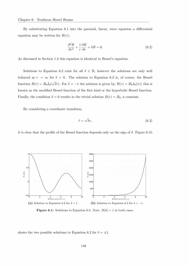
Chapter 6: Nonlinear Bessel Beams
By substituting Equation 6.1 into the paraxial, linear, wave equation a differential
equation may be written for B(r);
∂2B
∂r2+
1r
∂B
∂r+ δB = 0. (6.2)
As discussed in Section 1.2 this equation is identical to Bessel’s equation.
Solutions to Equation 6.2 exist for all δ ∈ R, however the solutions are only well
behaved as r → ∞ for δ > 0. The solution to Equation 6.2 is, of course, the Bessel
function B(r) = B0J0(√
δr). For δ = −1 the solution is given by, B(r) = B0J0(ir); this is
known as the modified Bessel function of the first kind or the hyperbolic Bessel function.
Finally, the condition δ = 0 results in the trivial solution B(r) = B0, a constant.
By considering a coordinate transform,
r =√
δr, (6.3)
it is clear that the profile of the Bessel function depends only on the sign of δ. Figure 6.1b
0 2 4 6 8 10−0.5
0
0.5
1
Radial position (r)
Pro
file
(a) Solution to Equation 6.2 for δ = 1.
0 2 4 6 8 100
500
1000
1500
2000
2500
3000
Radial position (r)
Pro
file
(b) Solution to Equation 6.2 for δ = −1.
Figure 6.1: Solutions to Equation 6.2. Note: B(0) = 1 in both cases.
shows the two possible solutions to Equation 6.2 for δ = ±1.
148

6.2 Nonlinear Bessel functions
Linear Nonlinearδ > 0 Bessel beam (J0(r)) Nonlinear Bessel beam (A(r))δ < 0 Modified Bessel beam (I0(r)) Townes profile (Rn(r))δ = 0 Trivial solution (B0) Nonlinear Bessel beam (A(r))
Table 6.1: Stationary solutions
6.1.1 A nonlinear Bessel equation
As was discussed in Section 4.1.3 the Nonlinear Schrodinger Equation (NSE) permits
stationary solutions of the form
u(r, z) = A(r) exp(iδz). (6.4)
By substituting Equation 6.4 into the NSE Equation 2.36 a differential equation may
be written for A(r);∂2A
∂r2+
1r
∂A
∂r+ δA + A3 = 0. (6.5)
where A ∈ R. Unlike Equation 6.2 well behaved solutions to Equation 6.5 exist for all
values of δ.
The Townes soliton (Section 4.1.3) exists as ground state solution to Equation 6.5
given δ < 0 and may be solved as a boundary value problem given the initial boundary
conditions; ∂rA = 0 and A(∞) = 0.
For δ ≥ 0 Equation 6.5 resembles Bessel’s equation (Equation 6.2) with a nonlinear
term. The solutions to this equation form a continuous set of functions known as nonlinear
Bessel functions [97].
Unlike the linear Bessel equation, Equation 6.5 possesses an infinite set of solutions
dependent on the parameters δ and A0. By adopting the normalisation,
r =√
δr, A =1√δA, (6.6)
the δ may be factored out of Equation 6.5, leaving solutions that only depend on initial
amplitude A0 and the sign of δ. Two solutions to Equation 6.5 are shown in Figure 6.2.
149

Chapter 6: Nonlinear Bessel Beams
0 2 4 6 8 100
0.1
0.2
0.3
0.4
0.5
0.6
0.7
0.8
0.9
1
Radial position (r)
Pro
file
(a) Solution to Equation 6.5 for δ = 1.
0 2 4 6 8 10−0.4
−0.2
0
0.2
0.4
0.6
0.8
1
Radial position (r)
Pro
file
(b) Solution to Equation 6.5 for δ = −1.
Figure 6.2: Solutions to Equation 6.5
0 1 2 3 4 5−0.5
0
0.5
1
Radial position (r)
Pro
file
A(r
)/A
0
A0 = 1A0 = 2A0 = 3Linear
Figure 6.3: Radial profile of nonlinear Bessel functions along with a linear Bessel function forcomparison
150

6.2 Nonlinear Bessel functions
6.2 Nonlinear Bessel functions
In order to determine the profile of the nonlinear Bessel function, Equation 6.5 is solved
as a boundary value problem using Matlab’s bvp4c function, subject to the boundary
conditions at r = 0; A = A0, ∂rA = 0.
Figure 6.3 shows the radial profile for three nonlinear Bessel beams, along with a linear
Bessel beam for comparison. The inclusion of the nonlinear term in Bessel’s equation
causes a radial compression of the nonlinear Bessel function that increases with initial
amplitude A0.
6.2.1 Comparison with linear Bessel functions
Various techniques for comparing the nonlinear Bessel profile with the linear profile are
suggested by Johannisson et al. [34]. For√
δr << 1 an approximation may be made based
on an effective value of δ
A = A0J0
(√δ + A2
0r
). (6.7)
However, beyond this limit the approximation is poor and neither the power in the central
lobe nor the periodicity of the outer lobes are matched.
In Section 4.6.2 it was noted that the blowup and power for the Bessel-Gauss beam
may be described by the power in the central lobe of the beam, therefore it is sensible to
attempt to match linear and nonlinear Bessel beams also in terms of the power and profile
of the central lobe.
Central lobe power
The power in the central lobe of a zero-order Bessel beam may be written as
Pcent =πA2
0j20,1
δJ1(j0,1)2, (6.8)
where j0,1 is the first root of the Bessel function J0. By numerically determining the
power in the central lobe of a nonlinear Bessel beam, a similar linear Bessel beam may be
constructed from Equation 6.8. The profile of a linear and nonlinear Bessel profile for
equal power in the central lobe is shown in Figure 6.4. In this approximation the intensity
is closely matched in the region of the central lobe, however the period of the outer lobes
151

Chapter 6: Nonlinear Bessel Beams
0 0.5 1 1.5 2−0.5
0
0.5
1
Radial position (r)
Pro
file
LinearNonlinear
Figure 6.4: Comparison of linear and nonlinear Bessel beams of equal power in the central lobe.
does not match up. This may lead to a variation in the cone angles between the two
beams.
Carrier frequency
Another method for matching up a nonlinear Bessel beam to its linear counterpart is to
make the frequency of the higher-order lobes to coincide. For a Bessel beam the asymptotic
form for r >> 1 goes as
J0(r) '√
2πr
cos(r − π
4
). (6.9)
By numerically measuring the spacing between successive maxima for the nonlinear Bessel
beam the characteristic spacing appears to converge on ∆r = 4.44. Therefore a similar
linear Bessel beam may be written as;
B(r) = J0
(∆r
2πr
). (6.10)
Figure 6.5 compares the central lobes for the linear and nonlinear Bessel beams frequency
matched in the outer lobes.
152

6.3 Nonlinear Bessel beams
0 0.5 1 1.5 2−0.5
0
0.5
1
Radial position (r)
Pro
file
LinearNonlinear
Figure 6.5: Comparison of linear and nonlinear Bessel beams for matched frequency in outerlobes.
6.3 Nonlinear Bessel beams
As with the linear counterpart, the nonlinear Bessel function does not represent a phys-
ically realisable beam profile as it also would carry an infinite amount of power. Some
truncation of the higher-order side lobes is required (Section 1.2.3).
Although it was stated in Section 6.1 that the nonlinear Bessel equation should tend
to zero as r →∞ it should be noted that this does not strictly imply finite power. If the
beam profile decays slower than r−1/2 then the power will remain unbounded; this is the
case for the linear Bessel function.
To prevent confusion the nomenclature of the various functions should be stressed
here. A linear Bessel profile is a solution to the linear Bessel equation Equation 6.2. The
initial condition for a linear Bessel-Gauss beam is the product of a Bessel function and a
Gaussian envelope. This remains a linear Bessel-Gauss beam irrespective of the medium
in which the beam propagates. When a linear Bessel-Gauss beam propagates in a Kerr-
like nonlinear material the periodic intensity modulation is observed in the direction of
propagation (Chapter 5).
A nonlinear Bessel profile is a solution to the nonlinear Bessel equation (Equation 6.5).
This may be used to form a nonlinear Bessel-Gauss beam by applying a Gaussian envelope
153

Chapter 6: Nonlinear Bessel Beams
Beam PowerLinear 18.4Nonlinear 16.7
Table 6.2: Full beam power, w0 = 30WFWHM .
of form;
u(r) = A(r) exp(− r2
w02
). (6.11)
Although the nonlinear Bessel beam is a stationary solution to the NLS, it does not
represent a real beam. If the nonlinear Bessel beam is truncated in order to ensure finite
power, then it is no longer strictly a stationary solution. By analogy to the linear Bessel
beam it is, however, hypothesised that the truncated nonlinear Bessel beam will exhibit
a high degree of localisation when compared to a beam such as a Gaussian of comparable
width to the central lobe.
6.3.1 Beam Power
To compare the linear and nonlinear Bessel beams, two profiles are chosen such that their
central lobe powers are matched (Section 6.2.1). The FWHM (indicated on Figure 6.4)
of the central lobe is similar for the two beams (WFWHM ' 0.8), therefore a Gaussian
envelope is applied with a width of w0 = 30WFWHM . The full beam powers for these
windowed beams are given in Table 6.2.
Although it has been asserted that the windowed nonlinear Bessel beam will not be a
truly stationary solution to the NSE, the precise behaviour of the beam must be investi-
gated numerically using a model such as HARP.
6.3.2 Numerical results
The intensity profiles for a nonlinear Bessel-Gauss beam (A0 = 1, δ = 1) and a linear
Bessel-Gauss beam, of equal central lobe powers and initial on-axis intensities, propagating
in a nonlinear medium are shown in Figure 6.6 and the axial intensities are shown in
Figure 6.8a. The linear Bessel-Gauss beam (Figure 6.6a) exhibits the periodic intensity
modulation discussed in Chapter 5, in addition to the intensity modulation the outer lobes
become distorted contracting slightly towards the beam centre.
Although the introduction of a Gaussian envelope means that the intensity profile
154

6.3 Nonlinear Bessel beams
for the nonlinear Bessel-Gauss beam – shown in Figure 6.6b – is no longer stationary,
the beam still exhibits the anticipated quasi-stationary behaviour. The most obvious
difference between the linear and nonlinear Bessel-Gauss beams is the absence of any
periodic modulation in the nonlinear Bessel-Gauss beam. Furthermore, the outer lobes
of the nonlinear Bessel-Gauss beam remain highly localised, and are not subject to the
distortion or periodic modulation experienced by the linear Bessel-Gauss beam.
Careful inspection of Figure 6.6b reveals that as the intensity of the nonlinear Bessel-
Gauss beam drops off, due to linear diffraction of the Gaussian envelope, the side lobes
experience a slight shift away from the beam centre.
Linear propagation
To compare the behaviour of the linear and nonlinear Bessel beams further, the propa-
gation is compared for a linear material. The intensity profiles are shown in Figure 6.7
and the axial intensity is shown in Figure 6.8b. In a linear medium the quasi stationary
behaviour of the linear Bessel-Gauss beam is restored. Predictably the nonlinear Bessel
beam no longer exhibits quasi stationary behaviour. The outer lobes appear to diffract
away from the beam centre. This behaviour is similar to the behaviour of the nonlinear
Bessel-Gauss beam in a nonlinear medium once linear diffraction has begun to dominate.
This suggests that the diffraction away from the beam centre experienced by the side
lobes in Figure 6.6b is caused by a decrease in intensity meaning the beam is becoming
less nonlinear.
155

Chapter 6: Nonlinear Bessel Beams
(a) Normalised intensity slice for a linear Bessel beam.
(b) Normalised intensity slice for a nonlinear Bessel beam.
Figure 6.6: Intensity profile for propagation in a Nonlinear medium
156

6.3 Nonlinear Bessel beams
(a) Normalised intensity slice for a linear Bessel beam.
(b) Normalised intensity slice for a nonlinear Bessel beam.
Figure 6.7: Intensity profile for propagation in a Linear medium
157
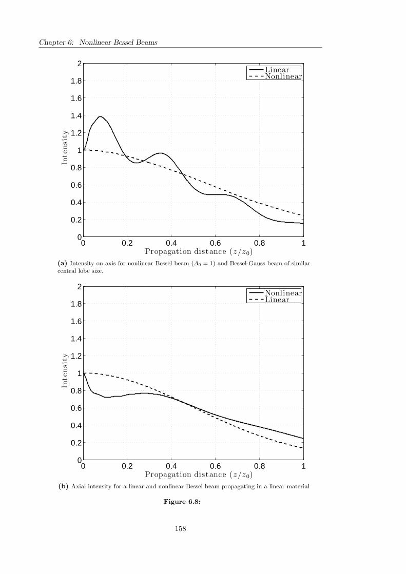
Chapter 6: Nonlinear Bessel Beams
0 0.2 0.4 0.6 0.8 10
0.2
0.4
0.6
0.8
1
1.2
1.4
1.6
1.8
2
Propagation distance (z/z0)
Inte
nsi
ty
LinearNonlinear
(a) Intensity on axis for nonlinear Bessel beam (A0 = 1) and Bessel-Gauss beam of similarcentral lobe size.
0 0.2 0.4 0.6 0.8 10
0.2
0.4
0.6
0.8
1
1.2
1.4
1.6
1.8
2
Propagation distance (z/z0)
Inte
nsi
ty
NonlinearLinear
(b) Axial intensity for a linear and nonlinear Bessel beam propagating in a linear material
Figure 6.8:
158

6.4 Nonparaxial nonlinear Bessel beams
6.3.3 Shaping nonlinear Bessel beams
In a similar manner to the linear Bessel beams discussed in Section 1.2.3 the axial be-
haviour of a nonlinear Bessel beam may be shaped by applying the appropriate envelope
to the beam profile. In Section 1.2.3 it was noted that applying a super Gaussian enve-
lope provided an extended flat region in the axial intensity. Figure 6.9 compares the
0 0.2 0.4 0.6 0.8 10
0.2
0.4
0.6
0.8
1
1.2
1.4
1.6
1.8
2
Propagation distance (z/z0)
Inte
nsi
ty
Bessel beamStationary beam
Figure 6.9: Axial intensity for linear and nonlinear Bessel beams with a super Gaussian envelope,p = 4.
axial intensity for a linear and nonlinear Bessel beam of equivalent central lobe powers
windowed with a super Gaussian function, p = 4. The linear Bessel beam exhibits the
intensity modulation discussed in Chapter 5.
6.4 Nonparaxial nonlinear Bessel beams
There also exists a set of nonlinear Bessel beams which may be derived from the Non-
paraxial Nonlinear Schrodinger Equation (NNSE) – introduced in Section 2.3,
κ∂2u
∂z2+ i
∂u
∂z+∇2
⊥u + |u|2u = 0. (6.12)
In an identical manner to the paraxial NSE, stationary solutions may be sought by sub-
stituting Equation 6.4 into Equation 6.12. Therefore, stationary solutions to the NNSE
159

Chapter 6: Nonlinear Bessel Beams
exists providing A(r) satisfies the differential equation;
∂2A
∂r2+
1r
∂A
∂r+(δ − κδ2
)A + A3 = 0. (6.13)
This equation yields two interesting results. Firstly, for δ(1 − κδ) < 0, the solution A(r)
resembles the Townes profile, Rn(r). This may occur when δ < 0 as with the paraxial
NSE, however this may also occur when κδ > 1. Both conditions imply that in real units
the forward phase evolution kz must be larger than the wave-number. For non-evanescent
waves this is only permitted in a nonlinear medium, which is consistent with the assertion
that no Townes-like soliton solutions exist for the linear wave equation.
For δ(1 − κδ) > 0 the nonlinear Bessel profile, discussed in Section 6.2, is obtained.
By introducing the coordinate transformation,
r =√
δ − κδ2r, A =1√
δ − κδ2A, (6.14)
it is clear that the stationary solutions to the NSE are also solutions to the NNSE subject
to the appropriate coordinate transformation given in Equation 6.14. The same beam
profile will evolve in the same manner under the NNSE as it would under the NSE, with
a slight variation in the phase; in the limit κ → 0 the evolution of the stationary profiles
are entirely identical.
Modelled using the difference differential method, with an inner cone angle of θ = 20◦,
the axial intensity for the nonparaxial nonlinear Bessel beam (shown in Figure 6.10) evolves
in an almost identical manner to the paraxial nonlinear Bessel beam (Figure 6.8a). This
confirms the existence of nonparaxial quasi-stationary solutions to the NNSE.
6.5 Higher-order nonlinear Bessel beams
By analogy to higher-order Bessel beams it is possible to demonstrate that a set of sta-
tionary solutions to the NSE exists for beams possessing azimuthal phase by considering
a field of the form,
u(r, θ, z) = A(r) exp(inθ) exp(iδz), (6.15)
160

6.5 Higher-order nonlinear Bessel beams
Figure 6.10: Comparison of axial intensity for nonparaxial linear and nonparaxial nonlinearBessel beams
where n ∈ N. By substituting Equation 6.15 into the NSE (Equation 2.36) a differential
equation may be written for A(r);
∂2A
∂r2+
1r
∂A
∂r+ δA− n2
r2A + A3 = 0. (6.16)
In the case of n = 0 Equation 6.5 is recovered. For n 6= 0 the azimuthal term in Equation
6.15 results in a point of undefined phase at r = 0, therefore the field must be zero at this
point; A(r = 0;n 6= 0) = 0.
6.5.1 Boundary conditions
For the zero-order nonlinear Bessel profile, symmetry was assumed about r = 0, however
this is not necessarily the case for higher-order profiles. Boundary conditions may be
determined by examining Equation 6.16.
In the limit r → 0 several terms of Equation 6.16 become difficult to evaluate, and an
alternative arrangement of this ODE is therefore required. By multiplying through by r2
the equation may be written as;
r2 ∂2A
∂r2+ r
∂A
∂r+ r2δA− n2A + r2A3 = 0. (6.17)
161

Chapter 6: Nonlinear Bessel Beams
Equation 6.17 is much easier to deal with in the limit r → 0, however in the limit r →∞
some of the terms may grow. Because of this, Equation 6.17 is used to determine boundary
conditions for Equation 6.16 which is in turn solved subject to these boundary conditions
to determine the nonlinear Bessel beam profile of order n.
Determining boundary conditions
Boundary conditions for B(r) may be determined by considering the derivatives of Equa-
tion 6.17. Differentiating Equation 6.17 with respect to r yields;
r2 ∂3A
∂r3+ 2r
∂2A
∂r2+
∂A
∂r+ r
∂2A
∂r2+ r2δ
∂A
∂r+ 2rδA− n2 ∂A
∂r+ 2rA3 + 2r2A2 ∂A
∂r= 0. (6.18)
If it is assumed that all higher-order derivatives are finite then all the terms involving r
may be eliminated in the limit r → 0. This leaves
∂A
∂r(1− n2) = 0. (6.19)
Therefore the first derivative in r may only be non-zero for n = 1.
Boundary conditions for n > 1
In order to determine the boundary condition for n ∈ N the previous technique may be
generalised as follows.
To determine the boundary condition for n = m Equation 6.17 must be differentiated
m times;∂m
∂rm
(r2 ∂2A
∂r2+ r
∂A
∂r+ r2δA− n2A + r2A3
)= 0. (6.20)
The generalised differentiation of a product may be written as follows;
∂m
∂rm(g(r)f(r)) =
m∑l=0
m!l!(m− l)!
∂l
∂rlg(r)
∂m−l
∂rm−lf(r). (6.21)
Equation 6.21 may be applied to the individual terms in Equation 6.20 to determine the
162
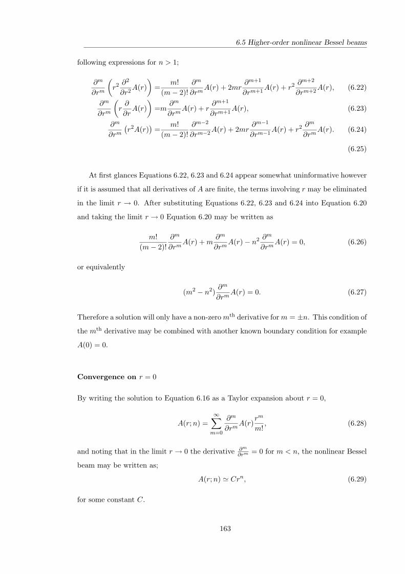
6.5 Higher-order nonlinear Bessel beams
following expressions for n > 1;
∂m
∂rm
(r2 ∂2
∂r2A(r)
)=
m!(m− 2)!
∂m
∂rmA(r) + 2mr
∂m+1
∂rm+1A(r) + r2 ∂m+2
∂rm+2A(r), (6.22)
∂m
∂rm
(r
∂
∂rA(r)
)=m
∂m
∂rmA(r) + r
∂m+1
∂rm+1A(r), (6.23)
∂m
∂rm
(r2A(r)
)=
m!(m− 2)!
∂m−2
∂rm−2A(r) + 2mr
∂m−1
∂rm−1A(r) + r2 ∂m
∂rmA(r). (6.24)
(6.25)
At first glances Equations 6.22, 6.23 and 6.24 appear somewhat uninformative however
if it is assumed that all derivatives of A are finite, the terms involving r may be eliminated
in the limit r → 0. After substituting Equations 6.22, 6.23 and 6.24 into Equation 6.20
and taking the limit r → 0 Equation 6.20 may be written as
m!(m− 2)!
∂m
∂rmA(r) + m
∂m
∂rmA(r)− n2 ∂m
∂rmA(r) = 0, (6.26)
or equivalently
(m2 − n2)∂m
∂rmA(r) = 0. (6.27)
Therefore a solution will only have a non-zero mth derivative for m = ±n. This condition of
the mth derivative may be combined with another known boundary condition for example
A(0) = 0.
Convergence on r = 0
By writing the solution to Equation 6.16 as a Taylor expansion about r = 0,
A(r;n) =∞∑
m=0
∂m
∂rmA(r)
rm
m!, (6.28)
and noting that in the limit r → 0 the derivative ∂m
∂rm = 0 for m < n, the nonlinear Bessel
beam may be written as;
A(r;n) ' Crn, (6.29)
for some constant C.
163

Chapter 6: Nonlinear Bessel Beams
6.5.2 Higher-order nonlinear Bessel profile
To determine, A(r;n = 1), Equation 6.16 is solved subject to the boundary conditions
that ∂rA = A0 and A(0) = 0. The profile A(r;n = 1) is shown in Figure 6.11 for
0 1 2 3 4 5−0.6
−0.4
−0.2
0
0.2
0.4
0.6
0.8
1
Radial position (r)
Pro
file
A(r
)/A
0
A0 = 1A0 = 2A0 = 3Linear
Figure 6.11: Radial profiles for higher-order nonlinear Bessel beams, n = 1
increasing values of A0. As with the n = 0 nonlinear Bessel beam, increasing A0 causes a
compression of the inner lobes.
6.5.3 Numerical results
As with the n = 0 nonlinear Bessel beams, the nonlinear Bessel beam for n > 0 must
also be truncated to ensure finite power; again this is achieved by applying a Gaussian
envelope. Due to the azimuthal phase, the intensity at r = 0 remains zero throughout
propagation.
The intensity profile for a linear Bessel-Gauss beam propagating in a nonlinear medium
is shown in Figure 6.12a. Although the beam does not appear to experience severe mod-
ulation in the direction of propagation – as is the case with the n = 0 Bessel-Gauss beam
– there is still significant distortion of the Bessel lobes as the beam evolves. For the non-
linear Bessel-Gauss beam – shown in Figure 6.12b – this distortion is eliminated and the
beam evolves in a quasi-stationary manner, as anticipated.
164
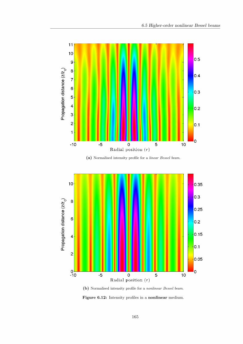
6.5 Higher-order nonlinear Bessel beams
(a) Normalised intensity profile for a linear Bessel beam.
(b) Normalised intensity profile for a nonlinear Bessel beam.
Figure 6.12: Intensity profiles in a nonlinear medium.
165

Chapter 6: Nonlinear Bessel Beams
6.6 Conclusions
It is demonstrated that unlike the linear wave equation, the NSE permits stationary solu-
tions for both positive and negative eigenvalues (δ). For δ < 0 this results in the Townes
soliton (Section 4.1.3), however for δ > 0 this results in a set of solutions known as non-
linear Bessel functions, so-called due to their similarity with the linear Bessel function.
However, unlike the linear Bessel function, the profile of the nonlinear Bessel functions are
unique to the amplitude A0.
As with the linear Bessel beam, the nonlinear Bessel beam also carries infinite power
and must therefore be truncated. In this chapter this is achieved by applying a Gaussian
or super-Gaussian window to the Bessel profile. This results in the beam no longer being a
true stationary beam, however a large region of quasi stationary behaviour is experienced
by the central lobe. None of the intensity modulation observed for the linear Bessel
beam (in Chapter 5) is present when the nonlinear Bessel beam is modelled in a Kerr-like
nonlinear material.
It is also demonstrated that just as the Bessel profile is a stationary solution to the
Helmholtz wave equation, the nonlinear Bessel profile is also a stationary solution to the
nonparaxial nonlinear Schrodinger equation.
It is demonstrated that there exists a set of stationary solutions for beams possessing
an azimuthal phase component. The boundary conditions to such stationary vortex beams
may be specified by the axial field and the nth derivative. It is suggested that the large
interaction length and stability of such beams may be applied to the manipulation of
particles in fluids exhibiting large nonlinearity such as benzene.
By analogy to linear Bessel beams it is possible that nonlinear Bessel beams exist for
non integer-orders of n, however the derivation of boundary conditions for such beams
would involve fractional differentiation. Furthermore it is likely that stationary solutions
exist in elliptical and parabolic co-ordinate systems.
166

Chapter 7
Conclusions
7.1 General conclusions
In Chapter 2 the nonlinear wave equation, the NSE was introduced; this wave equation
forms the basis for all of the paraxial beam propagation presented in this thesis. It was
noted that finite difference methods are ineffective for evaluating the NSE due to either
stability issues or poor efficiency. These techniques are therefore rejected in favour of a
symmetrised split step method as this delivers both improved stability and performance.
However, the performance of the symmetrised split-step method was shown to be still
inefficient for radially symmetric beam profiles as these must be evaluated using the two
dimensional FFT. The complexity of the problem was reduced by adopting a radially
symmetric co-ordinate system. Despite the relatively inefficient nature of the QDHT used
to evaluate the radial transform, this resulted in a model that was 40 times faster when
evaluating the evolution of a simple Gaussian beam. In order to sample the field on-axis
– something that is not possible with the zero-order QDHT – the generalised sampling
formula was applied for the first time to an optical model. This allowed the fast and
accurate reconstruction of a well sampled field at any point in r including the origin.
Despite the significant improvement gained by adopting radially symmetric co-ordinates,
further improvements were still made. An adaptive step length was introduced that al-
lowed the local error to be maintained within acceptable bounds. This adaptive step
length typically resulted in a doubling of the model speed but did so without sacrificing
accuracy.
It was noted that for highly nonlinear problems the beam width in frequency space
167
Chapter 7: Conclusions
may grow rapidly. To allow the model to cope with this, an adaptive grid was introduced.
Although this adaptive grid did not result in a significant improvement for the Gaussian
beam below the critical power, it was demonstrated that for the more exotic Bessel-Gauss
beam profile the adaptive grid improved the model speed by nearly a factor of two.
By combining the two adaptive techniques the Hankel-based Adaptive Radial Propaga-
tor (HARP) was developed. This provided not only the improvements in speed discussed
above but removed the need for the careful selection of initial grid size and step length.
For beams close to and above the critical power it was shown that the local error and
beam width in frequency space increase rapidly as the beam approaches the point of self-
focusing. In these situations HARP was able to quickly approach the point of self-focusing
before simultaneously increasing the grid and reducing the step length.
Owing to this ability to quickly and accurately investigate the point of critical self-
focusing, HARP was used in Chapter 4 to investigate the boundary between global exis-
tence and the two forms of critical self-focusing, blowup and collapse. Previously, most of
the work on critical self-focusing has been highly mathematical. This chapter presented
critical self-focusing in the NSE in more accessible fashion.
A technique was developed for numerically evaluating the beam fate using HARP for
arbitrary radially symmetric beam profiles. By comparing the obtained critical power for
a Gaussian beam with previously determined values it was demonstrated that HARP is
a highly accurate tool, well suited for the study of critical self-focusing. This allowed the
beam fate for the more complicated Bessel-Gauss beam to be studied with confidence. By
evaluating the semi-analytic sufficient conditions for global existence and collapse it was
shown that the region of parameter space that was not defined by sufficient conditions was
considerably larger for the Bessel-Gauss beam. Furthermore, unlike the Gaussian beam,
it was observed that the behaviour was dependent on the width of the Gaussian envelope.
By numerically investigating the unknown region it was shown that the boundary
between blowup and collapse appeared as expected, however, the boundary between global
existence and blowup was far less predictable. For certain regions of parameter space,
increasing the beam power actually prevented the beam from collapsing, such behaviour
has not been demonstrated before in the NSE.
For powers below the critical power for blowup, the behaviour of the Bessel-Gauss
beam was investigated in Chapter 5. This chapter built on the work of [35, 36, 98] and
168

7.1 General conclusions
demonstrated that the existing equation describing the modulation length was inaccurate
and that in fact the observed modulation length varied with beam power. A modification
was proposed yielding a power dependent beat length equation that accurately describes
the modulation length in both the paraxial and quasi-nonparaxial regimes.
Furthermore, it was noted that as the axial intensity decays the intensity modulation
appeared to become negatively chirped. By combining the modified beat length equation
with the linear axial intensity it was shown that this chirp is caused by the decay in
intensity from linear diffraction as the beam propagates. This led the assertion that by
shaping the windowing function, some control may be placed over the chirped intensity
modulation. It was demonstrated that a super Gaussian window may be used to produce
a more constant period of intensity modulation.
By including a low power Gaussian beam of comparable width to the central lobe it
was shown that the positions of the maxima and minima may be adjusted by varying
the phase of the Gaussian seed relative to the Bessel-Gauss beam; it was found that a
variation of 0 to π was sufficient to adjust the position of the maxima by a half period.
In the situation where the Bessel-Gauss beam was modelled passing through the full
focal length, rather than just starting from the focal point, it was observed that the
amplitude of intensity modulation was considerably reduced for the same beam power.
This was accompanied by an increase in average intensity. When this increased average
intensity was taken into account the observed modulation length was found to be in
agreement with the modified beat length equation. By using a Gaussian seed, it was
shown that the amplitude of intensity modulation could be increased, however the focal
points needed to be offset to prevent a discontinuity in the beat-length.
Finally, it was shown that by analogy to the linear Bessel equation there also exists a
nonlinear Bessel profile. This nonlinear Bessel profile represents a stationary solution to
the NSE and NNSE. It was shown that truncated nonlinear Bessel beams display the same
quasi-stationary behaviour in a nonlinear medium that the linear Bessel beam exhibits in
a linear medium. Additionally it was shown that there also exists a set of higher-order
nonlinear Bessel beams, possessing an azimuthal phase term. Boundary conditions were
determined for these higher-order beams and it was demonstrated that they too are quasi
stationary in Kerr-like nonlinear media.
169

Chapter 7: Conclusions
7.2 Further work
This work has opened up several avenues of theoretical, numerical and experimental work
that may be worthy of further investigation; these are summarised here. In particular it
would be interesting to verify the findings of this thesis experimentally.
In this thesis the use of the numerical model, HARP, is limited to the study of beams
in Kerr-like nonlinear materials. However, the principles of adaptive step length and grid
size may also be applied to other nonlinear processes such as nonlinear absorption and
plasma defocusing, through simple modifications to the linear or nonlinear operators. By
adding these processes to the model it may be possible to further investigate the behaviour
of beams in HMO glasses. Furthermore it may be possible to add time dependency to the
model to allow investigation of the spatio-temporal behaviour of pulsed systems.
The work in Chapter 4 has, for the first time, suggested that increasing the power of
a beam may prevent collapse, however further work is required on this subject before this
may be confirmed. It may prove edifying to investigate the fate of the beams as w0 is
further increased to see if the behaviour is repeated. By increasing the resolution along
the boundary it may be possible to see if this feature continues to repeat at smaller scales
and test the validity of the isolated regions of collapse.
The effects of nonlinear absorption and saturable nonlinearity on the propagation of
a Bessel-Gauss beam have not been taken into account; these may play an important
secondary role in stabilising the beam against self-focusing. The behaviour of the Bessel-
Gauss beam may be studied in the presence of nonlinear absorption by modifying HARP
as was suggested above. Additionally, cases of extreme nonparaxiality have not been
investigated. If the beat length remains valid for very large cone angles (θ > 40◦) it may
be possible to create periodic structures with a longitudinal separation on the order of the
wavelengths transparent within the material.
The reshaping behaviour as the Bessel passes through focus is not yet fully understood
and it is suggested that this may be linked to the nonlinear Bessel profile, discussed in
Chapter 6. Further analytic work is needed to fully understand the exact dynamics in this
situation. Additionally, the variation in blowup power needs to be investigated analytically
and numerically.
There is also the potential for further analytic work on nonlinear Bessel beams. Al-
170

7.2 Further work
though by its very definition, a stationary beam may not experience critical self-focusing
it is likely that the truncated nonlinear Bessel-Gauss beam will experience blowup and
collapse for sufficient power. It is possible that this power may be significantly higher
than the linear Bessel-Gauss beam and could potentially lead to an alternative method
for writing waveguides in highly nonlinear materials. Stationary solutions may also exist
for other forms of the nonlinear Schrodinger equation. It is likely that other stationary
solutions to the NSE – for Kerr and other nonlinearity – may be derived for parabolic and
elliptical co-ordinate systems.
Many of the conclusions reached in this thesis are may be easily tested experimentally.
It would be most interesting to see if the periodic modulation discussed in Chapter 5
can indeed be harnessed to write periodic structures as is suggested. The validity of the
modified beat-length equation may also be investigated experimentally. By generating the
nonlinear Bessel beam using a spatial light modulator it would be possible to determine
if these beams display the anticipated quasi-stationary behaviour. Additionally, the crit-
ical power of these beams may be easily tested experimentally. Finally it would prove
interesting to investigate if the critical self-focusing behaviour for the Bessel-Gauss beam
– whereby increasing the power stabilised the beam – may be reproduced experimentally.
171

Chapter 7: Conclusions
172

Bibliography
[1] J. Siegel, J. M. Fernandez-Navarro, A. Garcıa-Navarro, V. Diez-Blanco, O. Sanz, and
J. Solis. Waveguide structures in heavy metal oxide glass written with femtosecond
laser pulses above the critical self-focusing threshold. Applied Physics Letters, 86,
2005.
[2] V. Dıez-Blanco, J. Siegel, and J. Solıs. Waveguide structures written in SF57 glass
with fs-laser pulses above the critical self-focusing threshold. Applied Surface Sci-
ence, 252:4523–4526, April 2006.
[3] Weijia Yang, Costantino Corbari, Peter G. Kazansky, Koichi Sakaguchi, and Is-
abel C. Carvalho. Low loss photonic components in high index bismuth borate glass
by femtosecond laser direct writing. Opt. Express, 16(20):16215–16226, 2008.
[4] V. R. Bhardwaj, E. Simova, P. B. Corkum, D. M. Rayner, C. Hnatovsky, R. S.
Taylor, B. Schreder, M. Kluge, and J. Zimmer. Femtosecond laser-induced re-
fractive index modification in multicomponent glasses. Journal of Applied Physics,
97(8):083102, 2005.
[5] Guangyu Li, Kim A. Winick, Ali A. Said, Mark Dugan, and Philippe Bado. Waveg-
uide electro-optic modulator in fused silica fabricated by femtosecond laser direct
writing and thermal poling. Opt. Lett., 31(6):739–741, 2006.
[6] Stewart E. Miller. Integrated optics: An introduction. The Bell Systems Technical
Journal, 48:2059–2069, 1969.
[7] P. Dainesi, L. Thevenaz, and Ph. Robert. Intensity modulation in two mach-zehnder
interferometers using plasma dispersion in silicon-on-insulator. Applied Physics B:
Lasers and Optics, 73(5):475–478, 2001.
173

BIBLIOGRAPHY
[8] E. Cantelar, R. E. Di Paolo, J. A. Sanz-Garcıa, P. L. Pernas, R. Nevado, G. Lifante,
and F. Cusso. Second-harmonic generation in zn-diffused periodically poled linbo3
channel waveguides. Applied Physics B: Lasers and Optics, 73(5):515–517, 2001.
[9] Robert G. Hunsperger. Integrated optics : theory and technology. Springer, 1991.
[10] Gines Lifante. Integrated Photonics. Wiley, 2003.
[11] E.L. Wooten, K.M. Kissa, A. Yi-Yan, E.J. Murphy, D.A. Lafaw, P.F. Hallemeier,
D. Maack, D.V. Attanasio, D.J. Fritz, G.J. McBrien, and D.E. Bossi. A review of
lithium niobate modulators for fiber-optic communications systems. Selected Topics
in Quantum Electronics, IEEE Journal of, 6:69–82, 2000.
[12] M. N. Armenise. Fabrication techniques of lithium niobate waveguides. Optoelec-
tronics, IEE Proceedings, 135:85–91, 1988.
[13] K.M. Davis, K. Miura, N. Sugimoto, and K. Hirao. Writing waveguides in glass with
a femtosecond laser. Optics Letters, 21:1729–1731, November 1996.
[14] L. Eldada, C. Xu, K. M. T. Stengel, L. W. Shacklette, and J. T. Yardley. Laser-
Fabricated Low-Loss Single-Mode Raised-Rib Waveguiding Devices in Polymers.
Journal of Lightwave Technology, 14:1704–+, July 1996.
[15] D. Homoelle, S. Wielandy, A. L. Gaeta, N. F. Borrelli, and C. Smith. Infrared-
photosensitivity in silica glasses exposed to femtosecondlaser pulses. Optics Letters,
24:1311–1313, September 1999.
[16] S. Nolte, M. Will, J. Burghoff, and A. Tuennermann. Femtosecond waveguide writ-
ing: a new avenue to three-dimensional integrated optics. Applied Physics A: Ma-
terials Science & Processing, 77(1):109–111, 2003.
[17] M. A. A. Neil, R. Juskaitis, M. J. Booth, T. Wilson, T. Tanaka, and S. Kawata.
Active aberration correction for the writing of three-dimensional optical memory
devices. Applied Optics, 41(7):1374–1379, 2002.
[18] S. S. Mao, F. Quere, S. Guizard, X. Mao, R. E. Russo, G. Petite, and P. Martin.
Dynamics of femtosecond laser interactions with dielectrics. Applied Physics A:
Materials Science & Processing, 79(7):1695–1709, 2004-11-12.
174

[19] B. Rethfeld. Free-electron generation in laser-irradiated dielectrics. Phys. Rev. B,
73(3):035101, Jan 2006.
[20] N. T. Nguyen, A. Saliminia, W. Liu, S. L. Chin, and R. Vallee. Optical breakdown
versus filamentation in fused silica by use of femtosecond infrared laser pulses. Opt.
Lett., 28(17):1591–1593, 2003.
[21] D. Coric, P. R. Herman, K. P. Chen, X. M. Wei, P. B. Corkum, V. R. Bhardwaj, and
D. M. Rayner. Contrasts in writing photonic structures with ultrafast and ultraviolet
lasers. In M. J. Digonnet, editor, Proc. SPIE Vol. 4638, p. 77-84, Optical Devices
for Fiber Communication III, Michel J. Digonnet; Ed., volume 4638 of Presented at
the Society of Photo-Optical Instrumentation Engineers (SPIE) Conference, pages
77–84, May 2002.
[22] A. Zoubir, L. Shah, K. Richardson, and M. Richardson. Practical uses of femtosecond
laser micro-materials processing. Applied Physics A: Materials Science & Processing,
77(2):311–315, 2003.
[23] Y. Kondo, K. Nouchi, T. Mitsuyu, M. Watanabe, P. G. Kazansky, and K. Hirao.
Fabrication of long-period fiber gratings by focused irradiation of infrared femtosec-
ond laser pulses. Optics Letters, 24:646–648, May 1999.
[24] Y. Sikorski, A.A. Said, P. Bado, R. Maynard, C. Florea, and K.A. Winick. Optical
waveguide amplifier in nd-doped glass written with near-irfemtosecond laser pulses.
Electronics Letters, 36:226–227, 2000.
[25] William H. Dumbaugh and Josef C. Lapp. Heavy-metal oxide glasses. Journal of
the American Ceramic Society, 75(9):2315–2326, 1992.
[26] Lezal Dimitrij, Pedlikova Jika, Kostka Petr, Jana Bludska, Marcel Poulain, and Jiri
Zavadil. Heavy metal oxide glasses: preperation and physical properties. Journal of
Non-Crystalline Solids, 284:288–295, 2001.
[27] I. Kang, T. D. Krauss, F. W. Wise, B. G. Aitken, and N. F. Borrelli. Femtosecond
measurement of enhanced optical nonlinearities of sulfide glasses and heavy-metal-
doped oxide glasses. Journal of the Optical Society of America B Optical Physics,
12:2053–2059, November 1995.
175

BIBLIOGRAPHY
[28] A. Zoubir, C. Lopez, M. Richardson, and K. Richardson. Femtosecond laser fabrica-
tion of tubular waveguides in poly(methyl methacrylate). Optics Letters, 29:1840–
1842, August 2004.
[29] W. Gawelda, D. Puerto, J. Siegel, A. Ferrer, A. Ruiz de la Cruz, H. Fernandez, and
J. Solis. Ultrafast imaging of transient electronic plasmas produced in conditions of
femtosecond waveguide writing in dielectrics. Applied Physics Letters, 93(12):121109,
2008.
[30] Elena D’Asaro, Schirin Heidari-Bateni, Alessia Pasquazi, Gaetano Assanto, Jose
Gonzalo, Javier Solis, and Carmen N. Afonso. Interaction of self-trapped beams in
high index glass. Opt. Express, 17(19):17150–17155, 2009.
[31] Yan Li, Wataru Watanabe, Kazuhiro Yamada, Taishi Shinagawa, Kazuyoshi Itoh,
Junji Nishii, and Yongyuan Jiang. Holographic fabrication of multiple layers of
grating inside soda–lime glass with femtosecond laser pulses. Applied Physics Letters,
80(9):1508 –1510, mar 2002.
[32] Fei He, Haiyi Sun, Min Huang, Jian Xu, Yang Liao, Zenghui Zhou, Ya Cheng,
Zhizhan Xu, Koji Sugioka, and Katsumi Midorikawa. Rapid fabrication of optical
volume gratings in foturan glass by femtosecond laser micromachining. Applied
Physics A: Materials Science & Processing, 2009.
[33] N. E. Andreev, I. A. Aristov, L. I. Polonskii, and L. N. Piatnitskii. Bessel beams
of electromagnetic waves - Self-induced effects and nonlinear structures. Zhurnal
Eksperimental noi i Teoreticheskoi Fiziki, 100:1756–1766, December 1991.
[34] Pontus Johannisson, Dan Anderson, Mietek Lisak, and Mattias Marklund. Nonlinear
Bessel beams. Optics Communications, 222:107, 2003.
[35] V. Pyragaite, K. Regelskis, V. Smilgevicius, and A. Stabinis. Self-action of Bessel
light beams in medium with large nonlinearity. Optics Communications, 257:139–
145, January 2006.
[36] B. B. Sevruk. Self-modulation of Bessel-Gaussian wave beams in a medium with
cubic nonlinearity. Journal of Applied Spectroscopy, 73:701–706, September 2006.
176
[37] M. K. Bhuyan, F. Courvoisier, P.-A. Lacourt, M. Jacquot, L. Furfaro, M. J. With-
ford, and J. M. Dudley. High aspect ratio taper-free microchannel fabrication using
femtosecond bessel beams. Opt. Express, 18(2):566–574, 2010.
[38] Eugenijus Gaizauskas, Egidijus Vanagas, Vygandas Jarutis, Saulius Juodkazis, Vy-
gantas Mizeikis, and Hiroaki Misawa. Discrete damage traces from filamentation of
gauss-bessel pulses. Opt. Lett., 31(1):80–82, 2006.
[39] J. Durnin, J. J. Miceli, and J. H. Eberly. Diffraction-free beams. Phys. Rev. Lett.,
58(15):1499–1501, Apr 1987.
[40] J. Durnin. Exact solutions for nondiffracting beams. I. The scalar theory. Journal
of the Optical Society of America A, 4:651–654, April 1987.
[41] Desheng Ding and Xiaojun Liu. Approximate description for Bessel, Bessel-Gauss,
and Gaussian beams with finite aperture. J. Opt. Soc. Am. A, 16(6):1286–1293,
1999.
[42] D. McGloin and K. Dholakia. Bessel beams: diffraction in a new light. Contemporary
Physics, 46:15–28, January 2005.
[43] F. Gori, G. Guattari, and C. Padovani. Bessel-Gauss beams. Optics Communica-
tions, 64(6):491 – 495, 1987.
[44] S. Ruschin. Modified Bessel nondiffracting beams. Journal of the Optical Society of
America A, 11:3224–3228, December 1994.
[45] K F Riley. Mathematical methods for physics and engineering. American journal of
physics, 67, 1999.
[46] Zbigniew Jaroszewicz and Javier Morales. Lens axicons: systems composed of a di-
verging aberrated lens and a perfect converging lens. J. Opt. Soc. Am. A, 15(9):2383–
2390, 1998.
[47] G. Indebetouw. Nondiffracting optical fields: some remarks on their analysis and
synthesis. J. Opt. Soc. Am. A, 6(1):150–152, 1989.
[48] Tomas Cizmar and Kishan Dholakia. Tunable Bessel light modes: engineering the
axial propagation. Opt. Express, 17(18):15558–15570, 2009.
177

BIBLIOGRAPHY
[49] Narupon Chattrapiban, Elizabeth A. Rogers, David Cofield, III Wendell T. Hill, and
Rajarshi Roy. Generation of nondiffracting Bessel beams by use of a spatial light
modulator. Opt. Lett., 28(22):2183–2185, 2003.
[50] J. Rogel-Salazar, G. H. C. New, and S. Chavez-Cerda. Bessel-Gauss beam optical
resonator. Optics Communications, 190(1-6):117 – 122, 2001.
[51] C. L. Tsangaris, G. H. C. New, and J. Rogel-Salazar. Unstable Bessel beam res-
onator. Optics Communications, 223(4-6):233 – 238, 2003.
[52] Antti Vasara, Jari Turunen, and Ari T. Friberg. Realization of general nondiffracting
beams with computer-generated holograms. J. Opt. Soc. Am. A, 6(11):1748–1754,
1989.
[53] Jeffrey A. Davis, E. Carcole, and Don M. Cottrell. Nondiffracting interference pat-
terns generated with programmable spatial light modulators. Appl. Opt., 35(4):599–
602, 1996.
[54] Jeffrey A. Davis, Jarod Guertin, and Don M. Cottrell. Diffraction-free beams gen-
erated with programmable spatial light modulators. Appl. Opt., 32(31):6368–6370,
1993.
[55] Miguel A. Bandres, Julio C. Gutierrez-Vega, and Sabino Chavez-Cerda. Parabolic
nondiffracting optical wave fields. Opt. Lett., 29(1):44–46, 2004.
[56] J. C. Gutierrez-Vega, M. D. Iturbe-Castillo, and S. Chavez-Cerda. Alternative for-
mulation for invariant optical fields: Mathieu beams. Optics Letters, 25:1493–1495,
October 2000.
[57] Oleg V. Sinkin, Ronald Holzlohner, Ronald Holzl ohner, John Zweck, and Curtis R.
Menyuk. Optimization of the split-step fourier method in modeling optical-fiber
communications systems. J. Lightwave Tech., 21(1):61–68, 2000.
[58] G. P. Agrawal. Nonlinear Fiber Optics. Academic Press, 2001.
[59] Robert W.Byod. Nonlinear Optics. Academic Press, second edition edition, 2003.
[60] P. L. Kelley. Self-focusing of optical beams. Phys. Rev. Lett., 15(26):1005–1008, Dec
1965.
178

[61] G. Baruch, G. Fibich, and Semyon Tsynkov. Simulations of the nonlinear helmholtz
equation: arrest of beam collapse, nonparaxial solitons and counter-propagating
beams. Opt. Express, 16(17):13323–13329, 2008.
[62] P. Chamorro-Posada, G. S. McDonald, and G. H. C. New. Nonparaxial solitons.
Journal of Modern Optics, 45(6):1111–1121, 1998. 0950-0340.
[63] P. Chamorro-Posada, G. S. McDonald, and G. H. C. New. Non-paraxial beam
propagation methods. Optics Communications, 192:1–2, May 2001.
[64] W Press, S Teukolsk, W Vetterlin, and B Flannery. Numerical recipes in C++.
Cambridge University press, 2002.
[65] Thiab R. Taha and Mark I. Ablowitz. Analytical and numerical aspects of certain
nonlinear evolution equations. ii. numerical, nonlinear schrodinger equation. Journal
of Computational Physics, 55(2):203 – 230, 1984.
[66] R. Gadonas, V. Jarutis, R. Paskauskas, V. Smilgevicius, A. Stabinis, and
V. Vaicaitis. Self-action of Bessel beam in nonlinear medium. Optics Communi-
cations, 196(1-6):309–316, 2001.
[67] A Cloot, B.M Herbst, and J.A.C Weideman. A numerical study of the nonlinear
schrodinger equation involving quintic terms. Journal of Computational Physics,
86(1):127 – 146, 1990.
[68] Georgios D. Akrivis, Vassilios A. Dougalis, and Ohannes A. Karakashian. On
fully discrete Galerkin methods of second-order temporal accuracy for the nonlinear
Schrodinger equation. Numerische Mathematik, 59(1):31–53, 12 1991.
[69] J. A. Fleck, J. R. Morris, and M. D. Feit. Time-dependent propagation of high
energy laser beams through the atmosphere. Applied Physics A: Materials Science
& Processing, 10(2):129–160, 1976.
[70] M. D. Feit and J. A. Fleck, Jr. Light propagation in graded-index optical fibers.
Applied Optics, 17:3990–3998, December 1978.
[71] Gadi Fibich and Semyon Tsynkov. High-order two-way artificial boundary conditions
for nonlinear wave propagation with backscattering. J. Comput. Phys., 171(2):632–
677, 2001.
179

BIBLIOGRAPHY
[72] G. Fibich and S. Tsynkov. Numerical solution of the nonlinear helmholtz equation
using nonorthogonal expansions. Journal of Computational Physics, 210(1):183 –
224, 2005.
[73] Gadi Fibich. Small beam nonparaxiality arrests self-focusing of optical beams. Phys.
Rev. Lett., 76(23):4356–4359, Jun 1996.
[74] Li Yu, Meichun Huang, Mouzhi Chen, Wenzhong Chen, Wenda Huang, and Zhizhong
Zhu. Quasi-discrete Hankel transform. Opt. Lett., 23(6):409–411, 1998.
[75] Manuel Guizar-Sicairos and Julio C. Gutierrez-Vega. Computation of quasi-discrete
Hankel transforms of integer order for propagating optical wave fields. Journal of
the Optical Society of America. A, Optics, image science, and vision, 21(1):53–8,
2004. 1084-7529.
[76] Victor Namias. Fractionalization of Hankel transforms. IMA J Appl Math,
26(2):187–197, 1980.
[77] Matteo Frigo and Steven G. Johnson. The design and implementation of FFTW3.
Proc. IEEE, 93(2):216–231, 2005.
[78] P.P. Banerjee, G. Nehmetallah, and M.R. Chatterjee. Numerical modeling of cylin-
drically symmetric nonlinear self-focusing using an adaptive fast Hankel split-step
method. Optics Communications, 249(1-3):293 – 300, 2005.
[79] Pornsak Srisungsitthisunti, Okan K. Ersoy, and Xianfan Xu. Beam propagation
modeling of modified volume Fresnel zone plates fabricated by femtosecond laser
direct writing. J. Opt. Soc. Am. A, 26(1):188–194, 2009.
[80] Andrew W. Norfolk and Edward J. Grace. New beat length for writing periodic
structures using Bessel beams. Optics Communications, 283(3):447 – 450, 2010.
[81] H. P. Kramer. A generalized sampling theorem. Journal of Mathematics and Physics,
38:68–72, 1959.
[82] Abdul J. Jerri and Dale W. Kreisler. Sampling expansions with derivatives for finite
Hankel and other transforms. SIAM Journal on Mathematical Analysis, 6(2):262–
267, 1975.
180

[83] L. L. Campbell. A comparison of the sampling theorems of Kramer and Whittaker.
Journal of the Society for Industrial and Applied Mathematics, 12(1):117–130, 1964.
[84] J. P. Boyd. Chebyshev and Fourier Spectral Methods. Dover Publications, 2001.
[85] P. A. Belanger. Self-focusing of Gaussian beams: an alternate derivation. Applied
optics, 22(9):1293, 1983. 0003-6935.
[86] G. Fibich and A. L. Gaeta. Critical power for self-focusing in bulk media and in
hollow waveguides. Optics Letters, 25:335–337, March 2000.
[87] Gadi Fibich and George Papanicolaou. Self-focusing in the perturbed and unper-
turbed nonlinear Schrodinger equation in critical dimension. SIAM Journal on Ap-
plied Mathematics, 60(1):183–240, 1999.
[88] J Juul Rasmussen and K Rypdal. Blow-up in nonlinear Schrø”dinger equations-I a
general review. Physica Scripta, 33(6):481, 1986.
[89] George B. Arfken, Hans J. Weber, and Lawrence Ruby. Mathematical methods for
physicists, 4th ed. American Journal of Physics, 64(7):959–959, 1996.
[90] V. Vaicaitis, A. Stabinis, A. Marcinkevicius, and V. Jarutis. Second-order Stokes
and anti-Stokes coupling in stimulated Raman scattering by Bessel beam. Optics
Communications, 178(4-6):461–467, 2000.
[91] S. Sogomonian, L. Niggl, and Max Maier. Nonplanar phase-matching of stimulated
anti-Stokes Raman scattering pumped by a Bessel beam. Optics Communications,
162(4-6):261–266, 1999.
[92] R. Gadonas, V. Jarutis, A. Marcinkevicius, V. Smilgevicius, A. Stabinis, and
V. Vaicaitis. Transverse phase-matching in stimulated Raman scattering by a Bessel
beam. Optics Communications, 169(1-6):189–197, 1999.
[93] Surya P. Tewari, H. Huang, and R. W. Boyd. Theory of self-phase-matching. Phys.
Rev. A, 51(4):R2707–R2710, Apr 1995.
[94] Surya P. Tewari, H. Huang, and R. W. Boyd. Theory of third-harmonic generation
using Bessel beams, and self-phase-matching. Phys. Rev. A, 54(3):2314–2325, Sep
1996.
181

BIBLIOGRAPHY
[95] S. Sogomonian, S. Klewitz, and S. Herminghaus. Self-reconstruction of a Bessel
beam in a nonlinear medium. Optics Communications, 139:313–319, February 1997.
[96] Arne Jensen and Anders la Cour-Harbo. Ripples in Mathematics Ripples in Mathe-
matics. Springer Verlag, 2001.
[97] Yoshinori Kametaka. On a nonlinear Bessel equation. Publications of the Research
Institute for Mathematical Sciences, 8(1):151–200, 1972.
[98] N. S. Kazak, E. G. Katranji, I. A. Utkin, A. A. Ryzhevich, and A. N. Khilo. Self-
diffraction of Bessel light beams in a nonlinear medium. Journal of Applied Spec-
troscopy, 71(5):697–701, 2004.
[99] E. Hansen. Fast Hankel transform algorithm. Acoustics, Speech, and Signal Pro-
cessing [see also IEEE Transactions on Signal Processing], IEEE Transactions on,
33(3):666–671, 1985. 0096-3518.
[100] H. Fisk Johnson. An improved method for computing a discrete Hankel transform.
Computer Physics Communications, 43(2):181–202, 1987.
[101] V. Magni. High-accuracy fast Hankel transform for optical beam propagation. Jour-
nal of the Optical Society of America. A, Optics and image science, 9(11):2031, 1992.
0740-3232.
[102] A. E. Siegman. Quasi fast Hankel transform. Optics letters, 1(1):13, 1977. 0146-9592.
[103] G. P. Agrawal and M. Lax. End correction in the quasi-fast Hankel transform for
optical propagation problems. Opt. Lett., 6(4):171–173, 1981.
182

Appendix A
Norms
A.1 Vector norms
The Lp norm of a vector x of length n may be written as
||x||p :=
n∑j=1
|xi|p1/p
. (A.1)
The infinite norm, ||x||∞, is also known as the maximum norm as the result is effectively
the maximum element in x
||x||∞ = max(|x1|, |x2|, . . . , |xn|). (A.2)
A.2 Function norms
The generalised Lp norm of a function u(r), where r ∈ RD, is given by
||u||p :=
∫RD
|u(r)|p dDr
1/p
. (A.3)
In this thesis the function norm is used to simplify expressions, for example the power of
an optical field u(x, y) may be written as P = 2π||u||22.
183

Chapter A: Norms
184
Appendix B
Transforms
B.1 Fourier Transform
The Fourier transform relates two functions, u(x) and U(kx) as;
U(kx) =
∞∫−∞
u(x) exp [−ikxx] dx (B.1)
and
u(x) =12π
∞∫−∞
U(kx) exp [ikxx] dkx. (B.2)
B.1.1 Fast Fourier Transform
The numerical grid for real space and frequency space for a FFT is defined as
xn = n∆x kn = n∆k (B.3)
where ∆x = X/N and K = 1/∆x and ∆k = K/N To prevent aliasing in the sampled
function; the function must be sampled above the Shanon-Nyquist limit.
The time taken to evaluate the Fourier transform using the FFT scales as O(N log(N)).
It is commonly, and falsely, believed that the most efficient way of evaluating the FFT
ensuring that the number of sample points is an integer power of two – such that N = 2k
where k ∈ N. This indeed true for some basic implementations of the FFT algorithm such
as those given in [64] for which the number of sample points must be an integer number of
185

Chapter B: Transforms
N Factors Time599 599 1001024 210 56600 23 × 3× 52 44
Table B.1: Time take to execute FFT
points however this is not true for all FFT algorithms. Many mathematical programing
languages such as Matlab and the GNU Scientific Libraries (GSL) use the Fastest Fourier
Transform in the West (FFTW) libraries.
Consequently, to make the most efficient use of the FFT the number of sample points
should be selected so that it may be factored into small prime numbers. An example of
this is given in Table B.1. The memory required to perform the FFT scales as N .
B.1.2 Two dimensional Fourier transforms
The two dimensional transform between the functions u(x, y) and U(kx, ky) is given by;
U(kx, ky) =
∞∫−∞
∞∫−∞
u(x, y) exp [−ikxx− ikyy] dxdy. (B.4)
This may be evaluated, numerically, by applying the FFT algorithm along the elements in
one dimension followed by the elements in the other dimension. For a square grid of size
N along one dimension the time taken to apply this transform will scale as O(N2 log N).
B.2 The Hankel Transform
Hankel transform is the radial equivalent of the Fourier transform which may be applied
to any function F (r, θ) = A(r)B(θ). This is useful for optical systems because it allows
us to model beams which are either radially symmetric or which have a fixed azimuthal
phase; U(r, θ) = A(r) exp(inθ).
B.2.1 Derivation from the Fourier transform
The Hankel transform may be derived directly from the two dimensional Fourier transform
F (kx, ky) =
∞∫−∞
∞∫−∞
f(x, y) exp [−i(xkx + yky)] dxdy (B.5)
186
B.3 Numerical Hankel Transforms
by assuming radial co-ordinates r and θ in real space and kr and φ in frequency space.
These are related to the cartesian co-ordinates as:
x = r cos θ kx = kr cos φ (B.6)
y = r sin θ ky = kr sinφ (B.7)
(B.8)
where r ∈ [0, inf] and θ ∈ [0, 2π]. Equation B.5 may then be re-written as;
∞∫0
2π∫0
exp [−irkr(cos θ cos φ + sin θ sinφ)] rdrdθ (B.9)
∞∫0
2π∫0
exp [−irkr cos(θ − φ)] rdrdθ (B.10)
The Hankel transform represents a two dimensional Fourier transform for radially symmet-
ric systems. It may be derived directly from the Fourier transform by assuming radially
symmetric functions of form;
A(r, θ) = f(r) exp(inθ) (B.11)
The Hankel transform pairs are written as;
H{f(r)} = F (kr) =∫ ∞
0f(r)rJn(r.kr)dr (B.12)
and
H{F (kr)} = f(r) =∫ ∞
0F (kr)rJn(kr.r)dkr (B.13)
where Jn is the nth Bessel function. Note that, unlike the Fourier transform, the Hankel
transform and Inverse Hankel transform are identical.
B.3 Numerical Hankel Transforms
The numerical evaluation of the Hankel transform has been approached from several an-
gles, the two most common techniques are briefly discussed here for further reading on the
187

Chapter B: Transforms
other forms of numerical Hankel transform the reader is directed to [74, 75, 76, 99, 100,
101, 102].
The two Hankel transform techniques discussed here are the Quasi Fast Hankel Trans-
form (QFHT) by Siegman et al. [102] and the Quasi Discrete Hankel Transform (QDHT)
by Yu et al. [74].
B.3.1 Quasi Fast Hankel Transform
The Quasi Fast Hankel Transform (QFHT) exploits the highly efficient nature of the FFT
to evaluate the Hankel transform. The Hankel transform (Equation B.12) is transformed
into a two-sided cross-correlation integral which may be evaluated using the FFT. The
sample points for this transform are sampled at exponentially increasing points;
rn = r0 exp(αn)kr,m = kr,0 exp(αm) (B.14)
where n, m = 0, 1, ..., N − 1.
Each calculation for the QFHT takes 4N + log2(2N) complex multiplications. The
largest array for the QFHT has 2N points.
Although this method is extremely efficient, the method suffers from a central hole of
radius r0. Because of this hole it is necessary to chose a large number of sample points,
effectively sabotaging the efficient nature of the method. The technique of end correction
[103] may be applied to reduce the error from this hole, however this greatly restricts the
selection of parameters [74].
B.3.2 Quasi Discrete Hankel Transform
The Quasi discrete Hankel transform [74, 75] is computed from a unitary matrix and has
been shown to be faster than the QFHT for a given accuracy. The QDHT has a similar
order accuracy to the 2D FFT through both forward and reverse transforms, however
unlike the QFHT the QDHT requires N2 real multiplications followed by N2 summations.
The transform matrix is stored in a N×N matrix, however all other arrays required are of
length N . For a single transform the QDHT is highly inefficient due to the time required
to calculate the transform matrix, however for nonlinear beam modelling where the same
size transform is repeatedly applied the transform can be cached and re-used.
188

Appendix C
Fourier transform relations
C.1 Calculation of derivatives with the Fourier transform
The calculation of the derivative f ′(x) of a function f(x) bay be evaluated using the
Fourier transform;
F{f ′(x)
}=
∞∫−∞
f ′(x) exp(−ikxx)dx. (C.1)
This integral may be expanded using integration by parts;
∫u
∂v
∂xdx = [uv]−
∫v∂u
∂xdx (C.2)
where
∂v
∂x= f ′(x) (C.3)
u = exp(ikxx) (C.4)
this yields the equation
∞∫−∞
f ′(x) exp(−ikxx)dx = [f(x) exp(ikxx)]+∞−∞ −∞∫
−∞
f(x)ikx exp(−ikxx)dx (C.5)
For which f(x) vanishes at x = ±∞. Therefore
F{f ′(x)
}= ikxF {f(x)} (C.6)
189
Chapter C: Fourier transform relations
and
f ′(x) = F−1 {ikxF {f(x)}} (C.7)
which may be evaluated using the fast Fourier transform.
C.2 Calculation of exponentiatied derivative with the Fourier
transform
Some pseudo spectral methods such as the Split step method (Section 2.5.2) require the
calculation of exponentiated derivatives of the form;
exp[i
∂2
∂x2
]u(x). (C.8)
This may expressed as a Taylor expansion of the exponential function as;
exp[i
∂2
∂x2
]u(x) =
n=∞∑n=0
in
n!∂2n
∂x2nu(x). (C.9)
Using the Fourier transform relation for derivatives this may be expressed as
F{
exp[i
∂2
∂x2
]u(x)
}=
n=∞∑n=0
in(−1)n
n!k2n
x F {u(x)} . (C.10)
Which in turn may be written as;
exp[i
∂2
∂x2
]u(x) = F−1
{exp
[−ik2
x
]F {u(x)}
}(C.11)
190
Appendix D
Proof of error in split step method
D.1 Split step method
Using the notation from Section 2.5.2 for the linear, L and nonlinear N operator, the field
may be evaluated across one step of length ∆z using the split step method whereby the
propagation operator is approximated as
u(z + ∆z) = exp[∆z(L + n)
]= exp
(zL)
exp(zN)
+ ε (D.1)
where epsilon is an error incurred due to the non-commutation of the operators L and N .
The true operator may be expanded as follows
exp[∆z(L + N)
]= 1 + ∆z(L + N) +
∆z(L + N)2
2. . . (D.2)
= 1 + ∆zL + ∆zN +∆z2L2
2+
∆z2NL
2+
∆z2LN
2+
∆z2N2
2. (D.3)
This may be compared against the expansion of the split step operator
exp(∆zL
)exp
(∆zN
)=
(1 + ∆zL +
∆z2L2
2
)(1 + ∆zN +
∆z2N2
2
)(D.4)
= 1 + ∆zN +∆z2N2
2+ ∆zL + ∆z2LN +
∆z2L2
2. (D.5)
Where the terms of higher-order than ∆z2 have been discarded. By substituting the
expanded forms of Equation D.4 and Equation D.2 into Equation D.1 an expression for
191

Chapter D: Proof of error in split step method
the error may be determined;
ε = ∆z2
(LN − LN
2− NL
2
). (D.6)
Consequently the split step method has a lowest error term of O(∆z2) is second-order
accurate.
D.2 Symmetrised split step method
To increase the accuracy of the split step method, the symmetrised split step method may
be utilised (Section 2.5.2).
u(z + ∆z) = exp[∆z(L + N)
]= exp
(z
2N)
exp(zL)
exp(z
2N)
+ ε (D.7)
The expansion of the split step operator is given by
exp(z
2N)
exp(zL)
exp(z
2N)
=
(1 +
∆zN
2+
∆z2N2
8
)(1 + ∆zL +
∆z2L2
2
)
×
(1 +
∆zN
2+
∆z2N2
8
). (D.8)
(D.9)
If this is expanded then and terms of order O(∆z3) are truncated then we may write this
expansion as
exp(z
2N)
exp(zL)
exp(z
2N)
=1 + ∆zL + ∆zN +∆z2L2
2
+∆z2NL
2+
∆z2LN
2+
∆z2N2
2+ O(∆z3). (D.10)
By substituting this back into Equation D.7 then the error may be written as
ε = O(∆z3), (D.11)
and results in a third-order accuracy for the symmetrised split step method. This offers
improved accuracy over the split step method but requires twice as many applications of
192

D.2 Symmetrised split step method
the FFT algorithm.
193

194
Publications
• A. W. Norfolk, E. J. Grace
“Harnessing Self-Focusing: Direct Writing of Periodic Structures”, 8th Pacific Rim
Conference on Lasers and Electro-Optics, IEEE, Sept 2009
• A. W. Norfolk, E. J. Grace
“Harnessing Self-Focusing: Direct Writing of Periodic Structures”, Frontiers in Op-
tics (FiO), San Jose, California, October, 2009
• A. W Norfolk, E. J. Grace
“New beat length for writing periodic structures using Bessel beams”, Optics Com-
munications, 283(3), February 2010, pp(447-450)
• A. W Norfolk, E. J. Grace
“Reconstruction of optical fields with the Quasi-discrete Hankel transform”, Optics
Express 18(10), 2010, pp(10551-10556)
195