1

Beyond Rationality: Understanding Consumers’ Perceptions and Expectations of Inflation

Dr. Fabien Curto Millet Google

15 August 2012

Abstract While there exists an extensive literature seeking to directly test the rationality of inflation expectations, this paper has instead investigated whether consumers have rational perceptions of inflation in the first place. We argue that this is a necessary prerequisite to establish rationality, and its lack of consideration by much of the previous literature purporting to test rational expectations potentially casts doubts on its conclusions. Nevertheless, we find that the perceptions of inflation by consumers contain significant biases relative to official measures of inflation, and that their expectation forecasts fall short of what might be labelled rational even after controlling for the biases found. The biases are attributed to a number of factors that might shape consumers’ understanding of inflation. Beyond those factors, it is clear that consumers do not operate in a vacuum of information, and have regular access to the forecasts of economic experts through the news media. We therefore proceed to studying the relationship between consumer and professional expectations in Europe, following Carroll’s (2003) work with US data. On the whole, our results were unable to evidence a clear-cut picture of information being transmitted from experts to consumers for most countries, with however the salient exception of the UK, for which a very clear such mechanism was evidenced. We discuss possible reasons for the similarity between the UK and US in this respect, and relevant differences that might set them apart from the other European countries considered.

The views expressed in this paper are solely my own and do not necessarily reflect those of Google. I would like to thank especially Professor John Muellbauer for his extraordinary support and numerous insightful discussions over the years. I am also extremely grateful for comments from Dr. Mark Williams, Professor Peter Sinclair, Dr. Chris Bowdler, Dr. James Forder and Professor David Vines. Any errors are my own.

2

1. Introduction

The idea of “rational expectations” is due to Muth (1961) who hypothesised that “expectations, since they are informed predictions of future events are essentially the same as the predictions of the relevant economic theory”. In this view, agents’ subjective expectations of economic variables coincide with the objective mathematical conditional expectations of those variables: agents know the true underlying model of the economy and use it to inform their expectations. The popularity of this method in economic research followed both from its simplicity and the appealing idea that it concerns economically “intelligent” agents that avoid systematic mistakes1. Given its extensive use and the sensitivity of model outcomes to the use of rational expectations, much of the empirical work using direct measures of inflation expectations from surveys over the last thirty to forty years has focused on testing rational expectations – indeed, this has until recently been the predominant use of such data. A variety of countries, surveys, types of data (qualitative and quantitative), quantification methodologies (where applicable) and econometric techniques have been brought to bear on the question – usually (but not always) to conclude that one feature or the other associated with rational expectations is rejected by the data2. Yet, despite the build up of empirical evidence challenging it, the rational expectations paradigm continues to be a feature in recent models, such as in many variants of the New Keynesian Phillips Curve (Mankiw and Reis, 2002). In an effort to move the debate forward, this paper will challenge the rational expectations paradigm from a different angle: by examining whether consumers have rational perceptions of inflation in the first place (Section 3). We argue that this is a necessary prerequisite, and its lack of consideration by much of the previous literature purporting to test rational expectations potentially casts doubts on its conclusions. We find however that the apparent failure of rational expectations remains, and discover on the way a number of biases in the manner consumers understand inflation. Consumers however do not operate in a vacuum of information, and have regular access to the forecasts of economic experts through the news media. Section 4 explores the influence of professional forecasters in the formation of consumer inflation expectations. Before discussing the substance, however, we briefly introduce the survey data that this paper relies on in Section 2. Section 5 will offer concluding remarks. 2. Presentation of the survey data used

The present paper relies on direct measurements of inflation expectations and perceptions arising from three consumer surveys: the European Commission’s Consumer Survey; the Gallup survey in the UK; and the HIP survey in Sweden. We also rely on one survey of professional forecasters run by Consensus Economics for Section 4.

1 How successful they are at this depends on how much information one includes in the model put in the agents’ possession in the Muth (1961) definition; in particular, a weak definition of rationality would exclude knowledge of regime shifts from the model, which could lead to systematic prediction errors (Cukierman, 1986). 2 See inter alia: Roberts, 1997; Bakhshi and Yates, 1998; Łyziak, 2003; Nielsen (2003b); Forsells and Kenny (2006); Baghestani (1992); Hanssens and Vanden Abeele (1987); Figlewski and Wachtel (1981, 1983); Engsted (1991); Gerberding (2001, 2006); Thomas (1999); Papadia (1983); Kokoszczyński, Łyziak and Stanisławska (2006).

3

2.1. European Commission Consumer Survey

Participants to the European Commission’s Consumer Survey are asked the questions set out in Table 1, which yield data that is qualitative in nature. In order to quantify it, we use a variation of the Carlson Parkin methodology (Carlson and Parkin, 1975; Batchelor and Orr, 1988; Berk, 1999) proposed in Curto Millet (2004). In broad terms, the Carlson Parkin approach relies on making an assumption regarding the shapes of the aggregate distributions of expectations and perceptions. In our case, the assumption of normality was retained due to theoretical justifications through central limit theory and satisfactory performance in previous empirical work (Berk, 1999; Nielsen, 2003a).

TABLE 1: EC CONSUMER SURVEY, QUESTIONS 5 AND 6

Q5. How do you think that consumer prices have developed over the last 12 months? They have…

Q6. By comparison with the past 12 months, how do you expect that consumer prices will develop in the next 12 months? They will …

1 risen a lot 1 increase more rapidly 2 risen moderately 2 increase at the same rate 3 risen slightly 3 increase at a slower rate 4 stayed about the same 4 stay about the same 5 fallen 5 fall 9 don’t know. 9 don’t know. The shares of responses falling in each answer category in Table 1 are then interpreted as maximum likelihood estimates of areas under the aggregate density function of inflation expectations, that is, as probabilities. An estimate of mean expectations and perceptions can then be derived by exploiting the linkage between both questions, and using a measure of actual inflation as a scaling factor for mean inflation perceptions3. 2.2. The Gallup survey for the UK

Social Surveys (Gallup Poll) Ltd carried out a monthly survey on a sample of employees in the United Kingdom continuously between January 1983 and January 1997. The results of this were published in the Gallup Political Index reports, subsequently renamed Gallup Political and Economic Index reports. The responses required were of a quantitative nature. Gallup published the average survey response monthly, which is the series that will be used in what follows. The precise question asked was:

Over the next twelve months, what do you think the rate of inflation will be? 2.3. The HIP consumer survey for Sweden

The Households’ Purchasing Plans survey (Hushållens Inköpsplaner in Swedish, or HIP) has included quantitative questions on inflation expectations and perceptions on a quarterly basis between 1979q1 and 1992q4, the frequency becoming monthly from January 1993 onwards. With Sweden’s entry into the EU and the subsequent questionnaire harmonisation that took place, the survey started to include the standard EC qualitative questions on inflation 3 Please refer to Curto Millet (2007) for details.

4

perceptions and expectations (in addition to the quantitative ones) from January 1996. The quantitative questions included in the HIP survey have the following phrasing

TABLE 2: HIP SURVEY, INFLATION QUESTIONS

Concept Question:

Perceptions Compared with 12 months ago, how much higher in percent do you think that prices are now?

Expectations Compared with today, by what percentage do you think that prices will go up (i.e. the rate of inflation 12 months from now)?

SOURCE: Konjunkturinstitutet, Hushållens Inköpsplaner – User Manual 2.4. Consensus Economics Forecasts

The London-based macroeconomics survey collects on a quarterly basis forecasts from a panel of professional forecasters4 for key macroeconomic variables – including consumer price inflation – for each of the following one to six quarters. The means of these forecasts are published in the firm’s Consensus Forecasts reports. The data available for the purposes of this paper starts in 1994q1 (Germany, France, UK, Italy) or 1994q4 (Netherlands, Spain, Sweden), in all cases ending in 2005q4. 3. The rational perceptions hypothesis

An implicit assumption in much of the literature is that when consumers think about prices, they conceptualise them in the same way as the statisticians compiling the consumer price index. That is, to reach their personal notion of “consumer prices”, they weigh expenditure components in their heads in the same way as they are weighed in the CPI. In other words, the CPI is their reference index for inflation. We refer to this as the “rational perceptions hypothesis”. This assumption is debatable, at the very least. For instance, survey participants might respond to questions by thinking of retail price inflation rather than headline inflation. Their responses might be biased towards goods inflation, as many services are consumed less frequently; this matters given the differences between sectoral inflation rates due to technological progress differentials, for instance. One-off, administrative payments that influence the official index may also be excluded from their assessment. The literature testing the rationality of expectations has therefore either: (1) implicitly assumed the validity of the rational perceptions hypothesis; or (2) tested a joint hypothesis of the rationality of both expectations and perceptions. This is potentially a grave concern. Indeed, differences between the actual reference index and CPI may lead to systematic deviations between inflation expectations and ex post observed inflation without this depending in any way on the ability of consumers to form predictions.

4 As an example, the following UK forecasters participated in the January 2006 edition of Consensus Forecasts: Barclays Capital, Lombard Street Research, Williams de Broe, Lloyds TSB Financial Markets, Goldman Sachs, Citigroup, Credit Suisse First Boston, DTZ Research, Experian Business Strategies, RBS Financial Markets, UBS, Morgan Stanley, ABN Amro, Confederation of British Industry, Global Insight, HBOS, ITEM Club, JP Morgan, Oxford – LBS, Cambridge Econometrics, Deutsche Bank, HSBC, ING Financial Markets, Lehman Brothers, Liverpool Macro Research, Schroders, Economic Perspectives.

5

3.1. Testing the hypothesis on quantitative survey data from Sweden

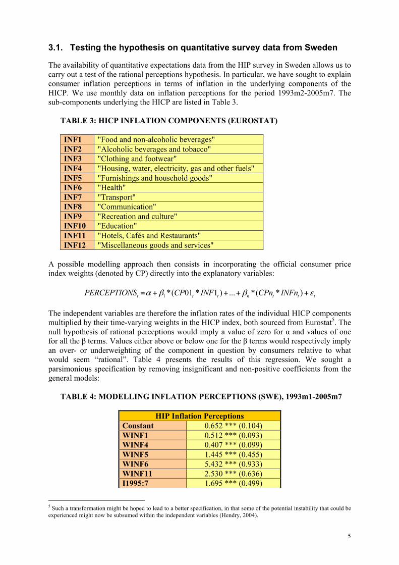
The availability of quantitative expectations data from the HIP survey in Sweden allows us to carry out a test of the rational perceptions hypothesis. In particular, we have sought to explain consumer inflation perceptions in terms of inflation in the underlying components of the HICP. We use monthly data on inflation perceptions for the period 1993m2-2005m7. The sub-components underlying the HICP are listed in Table 3.

TABLE 3: HICP INFLATION COMPONENTS (EUROSTAT) INF1 "Food and non-alcoholic beverages" INF2 "Alcoholic beverages and tobacco" INF3 "Clothing and footwear" INF4 "Housing, water, electricity, gas and other fuels" INF5 "Furnishings and household goods" INF6 "Health" INF7 "Transport" INF8 "Communication" INF9 "Recreation and culture" INF10 "Education" INF11 "Hotels, Cafés and Restaurants" INF12 "Miscellaneous goods and services"

A possible modelling approach then consists in incorporating the official consumer price index weights (denoted by CP) directly into the explanatory variables:

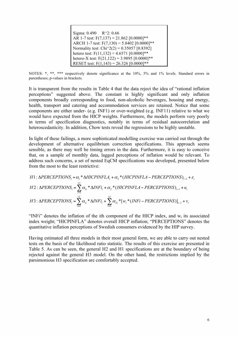
1 *( 01 * 1 ) ... *( * )t t t n t t tPERCEPTIONS CP INF CPn INFnα β β ε= + + + + The independent variables are therefore the inflation rates of the individual HICP components multiplied by their time-varying weights in the HICP index, both sourced from Eurostat5. The null hypothesis of rational perceptions would imply a value of zero for α and values of one for all the β terms. Values either above or below one for the β terms would respectively imply an over- or underweighting of the component in question by consumers relative to what would seem “rational”. Table 4 presents the results of this regression. We sought a parsimonious specification by removing insignificant and non-positive coefficients from the general models:

TABLE 4: MODELLING INFLATION PERCEPTIONS (SWE), 1993m1-2005m7

HIP Inflation Perceptions Constant 0.652 *** (0.104) WINF1 0.512 *** (0.093) WINF4 0.407 *** (0.099) WINF5 1.445 *** (0.455) WINF6 5.432 *** (0.933) WINF11 2.530 *** (0.636) I1995:7 1.695 *** (0.499)

5 Such a transformation might be hoped to lead to a better specification, in that some of the potential instability that could be experienced might now be subsumed within the independent variables (Hendry, 2004).

6

Sigma: 0.490 R^2: 0.66 AR 1-7 test: F(7,137) = 21.862 [0.0000]** ARCH 1-7 test: F(7,130) = 5.8402 [0.0000]** Normality test: Chi^2(2) = 0.35057 [0.8392] hetero test: F(11,132) = 4.6571 [0.0000]** hetero-X test: F(21,122) = 3.9895 [0.0000]** RESET test: F(1,143) = 26.326 [0.0000]**

NOTES: *, **, *** respectively denote significance at the 10%, 5% and 1% levels. Standard errors in parentheses; p-values in brackets. It is transparent from the results in Table 4 that the data reject the idea of “rational inflation perceptions” suggested above. The constant is highly significant and only inflation components broadly corresponding to food, non-alcoholic beverages, housing and energy, health, transport and catering and accommodation services are retained. Notice that some components are either under- (e.g. INF1) or over-weighted (e.g. INF11) relative to what we would have expected from the HICP weights. Furthermore, the models perform very poorly in terms of specification diagnostics, notably in terms of residual autocorrelation and heteroscedasticity. In addition, Chow tests reveal the regressions to be highly unstable. In light of these failings, a more sophisticated modelling exercise was carried out through the development of alternative equilibrium correction specifications. This approach seems sensible, as there may well be timing errors in the data. Furthermore, it is easy to conceive that, on a sample of monthly data, lagged perceptions of inflation would be relevant. To address such concerns, a set of nested EqCM specifications was developed, presented below from the most to the least restrictive:

1 2 112

1 2 11

12 12

1 2 11 1

1: * *( )

2 : * *( )

3: * *[ *( )]

t t t t

t i t t ti

t i t i i ti i

H PERCEPTIONS HICPINFLA HICPINFLA PERCEPTIONS

H PERCEPTIONS INFi HICPINFLA PERCEPTIONS u

H PERCEPTIONS INFi w INFi PERCEPTIONS

α α ε

α α

α α

−

−=

−= =

Δ = Δ + − +

Δ = Δ + − +

Δ = Δ + −

∑

∑ ∑ tv+

“INFi” denotes the inflation of the ith component of the HICP index, and wi its associated index weight; “HICPINFLA” denotes overall HICP inflation; “PERCEPTIONS” denotes the quantitative inflation perceptions of Swedish consumers evidenced by the HIP survey. Having estimated all three models in their most general form, we are able to carry out nested tests on the basis of the likelihood ratio statistic. The results of this exercise are presented in Table 5. As can be seen, the general H2 and H1 specifications are at the boundary of being rejected against the general H3 model. On the other hand, the restrictions implied by the parsimonious H3 specification are comfortably accepted.

7

TABLE 5: SWEDISH INFLATION PERCEPTIONS, NESTED TEST RESULTS Case No. Restrictions LogLik. Statistic Crit. value (5%) Result

General H3 vs General H2 11 19.50 19.68 Marginal non-

rejection General H3 vs

General H1 22 32.69 33.92 Marginal non-rejection

General H3 vs Specific H3 14 16.00 23.69 Do not reject

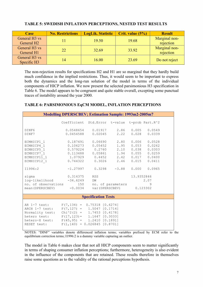
The non-rejection results for specifications H2 and H1 are so marginal that they hardly build much confidence in the implied restrictions. Thus, it would seem to be important to express both the dynamics and the long-run solution of the model in terms of the individual components of HICP inflation. We now present the selected parsimonious H3 specification in Table 6. The model appears to be congruent and quite stable overall, excepting some punctual traces of instability around the year 2000. TABLE 6: PARSIMONIOUS EqCM MODEL, INFLATION PERCEPTIONS

Modelling DPERSCBEV; Estimation Sample: 1993m2-2005m7 Coefficient Std.Error t-value t-prob Part.R^2 DINF6 0.0548654 0.01917 2.86 0.005 0.0549 DINF7 0.0454588 0.02045 2.22 0.028 0.0339 ECMHICP1_1 0.187491 0.06690 2.80 0.006 0.0528 ECMHICP4_1 0.106273 0.05452 1.95 0.053 0.0262 ECMHICP5_1 0.579224 0.2760 2.10 0.038 0.0303 ECMHICP7_1 0.113488 0.05861 1.94 0.055 0.0259 ECMHICP11_1 1.07929 0.4452 2.42 0.017 0.0400 ECMHICP12_1 0.744322 0.3026 2.46 0.015 0.0411 I1996:2 -1.27997 0.3298 -3.88 0.000 0.0965 sigma 0.314375 RSS 13.9352846 log-likelihood -34.6249 DW 2.07 no. of observations 150 no. of parameters 9 mean(DPERSCBEV) -0.0034 var(DPERSCBEV) 0.123302

Specification Tests AR 1-7 test: F(7,134) = 0.75318 [0.6274] ARCH 1-7 test: F(7,127) = 1.5047 [0.1714] Normality test: Chi^2(2) = 1.7453 [0.4178] hetero test: F(17,123)= 1.1647 [0.3033] hetero-X test: F(45,95) = 1.2410 [0.1891] RESET test: F(1,140) = 0.026845 [0.8701] NOTES: “DINF” variables denote differenced inflation terms; variables prefixed by ECM refer to the equilibrium correction terms; I1996:2 is a dummy variable capturing an outlier. The model in Table 6 makes clear that not all HICP components seem to matter significantly in terms of shaping consumer inflation perceptions; furthermore, heterogeneity is also evident in the influence of the components that are retained. These results therefore in themselves raise some questions as to the validity of the rational perceptions hypothesis.

8

3.2. Interpreting the rejection of the rational perceptions hypothesis

We now turn to exploring the rationale for certain HICP components being retained rather than others. Table 7 lists these components, whether kept as part of the dynamics, the long-run solution, or indeed both.

TABLE 7: HICP components retained in consumer inflation perceptions model

Code Concept Retained? INF1 "Food and non-alcoholic beverages" YES INF2 "Alcoholic beverages and tobacco" NO INF3 "Clothing and footwear" NO INF4 "Housing, water, electricity, gas and other fuels" YES INF5 "Furnishings and household goods" YES INF6 "Health" YES INF7 "Transport" YES INF8 "Communication" NO INF9 "Recreation and culture" NO INF10 "Education" NO INF11 "Hotels, Cafés and Restaurants" YES INF12 "Miscellaneous goods and services" YES

We hypothesise that the importance of a particular set of products in determining the inflation perceptions of consumers is increasing in the following four factors: 1. The frequency at which the prices in question are adjusted 2. The weight of these products in the overall expenditure of consumers 3. The level of inflation applicable to those products over the sample 4. The frequency at which the consumer purchases those products Table 8 provides data on some of these dimensions and computes a rough index of the ‘expected importance’ of particular components in consumer perceptions on the basis of this information. Unfortunately, it was not possible to find data on the fourth factor. Data on dimension 1 are based on the mean duration of prices by HICP component for Finland (Vilmunen and Laakkonen, 2004), collected and analysed in the context of the ECB’s Inflation Persistence Network. The use of Finnish data may be justified by the very similar HICP weights for both countries and great similarities in their industrial structure, business cycles and economic policies (as documented in Jonung and Sjöholm, 1999). The index of expected importance is computed as a percentage of the maximum attainable score. It is computed according to the following expression:

[1728 ( * * )] *1001727

FREQUENCY WEIGHT INFLATION ranksIMPINDEX −=

9

TABLE 8: MODELLING INFLATION PERCEPTIONS (SWE), 1993m1-2005m7

HICP Median Duration6

Frequency Rank

Avg HICP weight7

Weight Rank

Avg. Inflation (Abs. Value)8

Inflation Rank

Importance Index

(% Max)

Overall Rank

1 3.23 4 17.32% 2 0.41% 10 95.43% 3 2 4.30 6 5.78% 7 2.93% 2 95.19% 4 3 3.41 5 7.33% 5 0.54% 9 87.03% 7 4 3.10 3 19.15% 1 1.54% 6 99.02% 2 5 5.50 8 6.42% 6 0.99% 7 80.60% 10 6 6.30 10 1.68% 11 6.56% 1 93.69% 5 7 1.51 1 16.74% 3 2.64% 3 99.54% 1 8 1.80 2 3.16% 10 0.62% 8 90.79% 6 9 4.46 7 11.63% 4 0.21% 11 82.22% 8

10 23.33 12 0.18% 12 0.01% 12 0.00% 12 11 6.76 11 5.63% 8 2.09% 5 74.58% 11 12 5.96 9 4.97% 9 2.59% 4 81.30% 9

Table 8 provides some support for our hypothesised factors influencing inflation perceptions. As can be seen, our parsimonious EqCM model retained precisely the top three factors highlighted by our ‘expected importance’ index, namely: transport, food and non-alcoholic beverages, and housing/water/energy costs. The health component (importance rank 5) was also retained; this suggests that a component requires strength on one signal alone to be spotted by consumers. Indeed, this component ranks rather low in terms of either frequency of price adjustment or HICP weight; however, it has experienced almost twice as much inflation as any other sector over the period, making it a clear outlier in this respect. Our model has also retained certain components, despite relatively low importance scores above. The importance of the “hotels and catering services” component probably arises from the frequency at which the relevant products are purchased by consumers (almost certainly daily in the case of café and restaurant services), information that is missing from our index. The retention of the “furnishings and household goods” (component 5) and “miscellaneous goods and services” (component 12) is perhaps less clearly motivated. Component 5 essentially concerns a number of household durables, tools, maintenance and repairs as well as domestic and home care services. Component 12 notably includes personal care products and services (e.g. hairdressing), as well as banking and insurance services. The measures underlying Table 8 are by no means ideal. Moreover, we make no claim that each of these concepts (frequency, weight and inflation) ought to be aggregated with equal weights into an index of importance for consumer perceptions, as is implemented above. Notwithstanding this, the table appears to lend some support to our hypothesis on the determinants of consumer perceptions.

6 Median duration is an average for the years 1997-2003 and is expressed in months. Vilmunen and Laakkonen (2004) separated the sample for the years 1997-99 and 2000-03 for technical reasons which are not a concern here. The data concern Finland, as no similar data were available for Sweden. 7 HICP weights represent averages for the years 1990-2005. 8 The absolute value of average inflation is computed over the period 1993m1-2005m7.

10

3.3. Implication for assessments of the rationality of expectations

An immediate consequence of the foregoing analysis is that particular thought should be given to what is meant by the rational expectations hypothesis (“REH”), especially in the context of empirical tests thereof. Every study of the REH published to date to our knowledge essentially compares some measure of expectations with the actual outturns of inflation, as measured by official statistics. We have however just shown that consumers have an incomplete and possibly distorted view of what constitutes inflation, arguably dependent on a number of factors such as the frequency of price adjustment and purchases, expenditure weights and relative inflation of the underlying expenditure components. There is therefore no guarantee that the forecasts offered by consumers relate to the entirety of the CPI. In fact, there is rather a suspicion of the contrary, as the perceptions data used above were elicited with a question relating to prices in general. This casts doubt on the results and interpretation of past empirical studies of the rational expectations hypothesis. Indeed, given the above, the failure of consumer forecasts of CPI-type measures cannot but be expected – and results to the contrary seem a priori puzzling and may raise issues of sample-dependence. The relevant interpretation, however, need not be that consumers are making irrational forecasts too, as this issue is confounded with the additional null hypothesis that consumers have a correct understanding of inflation. It may be the case – although this is unlikely – that consumers make rational forecasts on the inflation index that they perceive. We now aim to check this conjecture empirically. We proceed by reweighting the components of HICP in a way that reflects their actual perceptions by consumers, thereby yielding a “perceptions-adjusted” inflation series (PAWINFLA). This is generated on the basis of the long-run solution to our specification in Table 6. We plot this perceptions-adjusted series against actual HICP inflation in Figure 1; the series appear to be closely related, although on occasions they do move in opposite directions.

FIGURE 1: PERCEPTIONS-ADJUSTED INFLATION VS HICP INLFATION

1995 2000 2005

0

2

4

6

8

10

12 HICPINFLA PAWINFLA

11

We then use the perceptions-adjusted inflation series as the anchor from which to derive the inflation expectations measure from the European Commission’s Consumer Survey evidence for Sweden, giving us an expectations measure we call “ADJEXPECT”. This differs from the standard quantification procedure for the EC Consumer Survey, which relies on the (unadjusted) official inflation rate, yielding an expectations measure we call “EXPECT”. This allows us to investigate the forecasting performance of our new expectations measure (“ADJEXPECT”) against future perceptions-adjusted inflation. This can be contrasted with: (i) the forecasting performance of a naïve benchmark which merely extrapolates the perceptions-adjusted inflation of the past 12 months ( exp

12, , 12t t t tπ π+ −= ); (ii) the forecasting performance of the standard expectations measure (“EXPECT”) on unadjusted HICP. Table 9 presents the results.

TABLE 9: COMPARATIVE FORECASTING PERFORMANCE, 1993m1-2005m7

Measure Period RMSE U1 % U2 % U3 % EXPECT 1997m1-2005m7 0.0107 7.3 6.1 86.6

ADJEXPECT 1997m1-2005m7 0.0092 22.90 19.94 57.16 Naïve 1997m1-2005m7 0.0067 0.38 23.18 76.43

As can be seen from the results, consumers appear to be little more rational in their forecasts than under traditional assessments of rationality despite these adjustments. The RMSE achieved here (0.0092) is only slightly improved relative to that which would be achieved without adjustments for perceptions biases (0.0107). Moreover, the finding that naïve forecasts outperform consumer expectations appears to be robust to these modifications. The last three columns of Table 9 relate to an interesting feature of the Mean Squared Error (MSE), which is that it can be decomposed into three insightful components (Clavería González, 2003). Let y denote inflation; bars placed over variables indicate averages, whereas hats ^ indicate the prediction of the variable for the relevant period. Hence, the expectation error in period t can be written as ˆ( )t t te y y= − and we have:

2 2 2 2 2ˆ ˆ

1

1 ˆ ˆ( ) ( ) (1 )T

t yy yyt

MSE e y y r rT

σ σ σ=

= = − + − + −∑

Where ˆyyr denotes the correlation coefficient between predicted and actual values, while σ̂ and σ correspond to the standard deviations of predictions and observations, respectively. The three components on the right hand side can be expressed as percentages by dividing through by the MSE: 1 = U1 + U2 + U3. These components have an intuitive interpretation. U1 refers to the proportion of MSE imputable to bias, being the square of the difference between the mean of predicted values and that of actual values. Since U2 depends on the difference between the standard deviations of predictions and actual values, it has an interpretation as the proportion of MSE due to dispersion, i.e. ‘regression error’. Finally, U3 arises from the lack of correlation between predictions and actual values and therefore represents the proportion of MSE due to all the factors that are unexplained or unaccounted for. In terms of this decomposition, the ideal outcome would be for the greatest weight to be achieved by the unexplained component of MSE, with a minimisation of systematic (U1) and regression error (U2). This provides us

12

with an additional criterion on which to assess our quantification measures. As can be seen in Table 9, the MSE decomposition for ADJEXPECT is also inferior to its standard counterpart EXPECT. 3.4. Conclusion

In view of the foregoing, we conclude that (i) consumers’ perceptions of inflation seem to be at odds with what one might expect from a Muthian interpretation of rationality given the biases they appear to display; and (ii) even controlling for these biases, the forecasts made by consumers do not appear to be particularly “rational” and are outperformed by naïve extrapolative forecasts. While we have explored in this section a number of factors that might shape consumers’ understanding of inflation (in the form of frequency of price changes/purchases, weight in expenditure basket and inflation levels by product category), it is certainly the case that consumers do not operate in a vacuum of information, and have regular access to the forecasts of economic experts through the news media. We explore this interaction in the following Section. 4. The expectations of consumers and economic experts

The present section proposes to develop our understanding of consumer inflation expectations by considering the way in which they might be influenced by the forecasts of professional forecasters and the diffusion of these through the mass media. Carroll (2003) made a pioneering contribution in this context in his study of US consumer expectations from the Michigan SRC survey and expert forecasts from the Survey of Professional Forecasters. We propose here to reconsider his findings in a European context, with a larger sample of seven countries, namely: France, Spain, Italy, the Netherlands, the UK, Sweden and Germany. We will rely on data from the EC Consumer Survey – quantified according to the methodology sketched in Section 2 – to obtain consumer inflation expectations, and use data from the “Consensus Forecasts” surveys to obtain the expectations of professional forecasters. The model proposed by Carroll (2003) can be interpreted as a microfoundation for that of Mankiw and Reis (2002). In essence, Carroll assumes that people obtain their macroeconomic views from information supplied in the media, which is absorbed probabilistically. In particular, the updating of expectations is assumed to follow the Calvo (1983) structure. Given this structure Carroll’s derivation eventually reaches the following equation: , 4 , 4 1 1, 3[ ] [ ] (1 ) [ ]t t t t t t t t tCONSEXP N CONSEXPπ λ π λ π+ + − − += + − Where CONSEXP denotes consumer expectations, and N denotes the forecasts reported in newspapers. The latter will be proxied by the data on expert forecasts, thus taking the view that these are reported and transmitted to the general public through the media. In what follows, we will: (i) compare the forecasting power of consumers and experts; (ii) consider the relationship between both sets of expectations; and (iii) explore the role of news coverage in the diffusion of expert forecasts and its implications in the context of the UK.

13

4.1. Comparing the forecasting power of consumers’ and experts’

expectations

We now compare the forecasting performance of consumers with that of professional forecasters on the basis of a range of descriptive statistics: the Mean Error (ME), RMSE and the MSE decomposition into factors U1, U2 and U3 described earlier. Table 10 presents the results. Consumer forecasts are contrasted with a CPI benchmark; expert forecasts based on the data from Consensus Economics are contrasted with the variable the professional forecasters were predicting (CPI in all cases except the UK, which uses several indices – RPI, RPIX and HICP – over the sample). A naïve benchmark is also provided, which simply predicts the same rate of inflation for the coming year as that observed over the previous year on the inflation measure used by Consensus Economics professional forecasters.

TABLE 10: PREDICTIVE ABILITY OF CONSUMERS AND EXPERTS CONSUMER FORECASTS Country ME RMSE U1 U2 U3 NOB France 0.0040 0.0067 35.0 8.9 56.1 44 Spain 0.0066 0.0123 28.8 37.8 33.3 41 Sweden 0.0028 0.0103 7.2 5.7 87.1 36 UK 0.0031 0.0099 9.7 37.4 52.9 44 Italy 0.0025 0.0085 8.3 13.3 78.5 44 Netherlands 0.0038 0.0085 19.2 6.9 73.9 41 Germany -0.0014 0.0086 2.6 63.5 33.9 44 EXPERT FORECASTS Country ME RMSE U1 U2 U3 NOB France -0.0005 0.0063 0.7 20.5 78.8 44 Spain 0.0014 0.0089 2.4 34.1 63.5 41 Sweden -0.0106 0.0154 46.6 14.4 39.0 41 UK -0.0015 0.0038 15.3 11.2 73.5 44 Italy 0.0021 0.0082 6.4 10.0 83.7 44 Netherlands 0.0006 0.0060 0.8 0.0 99.2 41 Germany -0.0022 0.0075 8.5 46.8 44.7 44 NAIVE FORECASTS Country ME RMSE U1 U2 U3 NOB France 0.0001 0.0061 0.0 28.2 71.7 44 Spain -0.0012 0.0095 1.6 45.6 52.8 41 Sweden -0.0020 0.0126 2.4 42.0 55.6 41 UK -0.0002 0.0068 0.1 49.8 50.2 44 Italy -0.0018 0.0098 3.4 24.1 72.5 44 Netherlands -0.0005 0.0085 0.4 27.6 72.0 41 Germany -0.0006 0.0073 0.6 51.8 47.6 44 As can be seen from the mean errors, expert forecasts are less biased than consumer forecasts in all but two countries (Sweden and Germany). Similarly, they are more accurate in RMSE terms for all countries but Sweden. We note that the qualitative findings in the Swedish case are not driven by the slightly different sample used for experts (starting in 1994q4) and

14

consumers (starting in 1996q1). The naïve forecasts beat both consumer and expert forecasts in terms of bias for every country; however, this does not translate straightforwardly into RMSE dominance. Table 11 summarises the situation by providing the average performance for each type of forecast.

TABLE 11: PREDICTIVE ABILITY OF CONSUMERS/EXPERTS, SUMMARY

Data Avg. ME Avg. RMSE Avg. U1 Avg. U2 Avg. U3 Consumer forecasts 0.0031 0.0093 15.8 24.8 59.4 Expert forecasts -0.0015 0.0080 11.5 19.6 68.9 Naïve forecasts -0.0009 0.0086 1.2 38.4 60.3 As could be expected, expert forecasts dominate in RMSE terms and also present the most favourable MSE decomposition. This result is in line with intuition. Nevertheless, their performance is surprisingly close to that of consumers and naïve measures, remaining well within the same order of magnitude. A question worthy of consideration is the extent to which these forecasts have further predictive power beyond that which is contained in past inflation data (Carroll, 2003). We examined this by regressing the inflation rate over the coming year on the inflation rate over the past year and either the consumer or expert inflation expectations, before running a non-nested test between both sets of forecasts. In terms of specification diagnostics, we considered a number of tests for these regressions, including: the Portmanteau (Q) test for white noise; Bartlett's periodogram-based test for white noise; the Breusch-Godfrey test for higher-order serial correlation; the Breusch-Pagan/Cook-Weisberg test for “general” heteroscedasticity and an LM test for autoregressive conditional heteroscedasticity; and finally, skewness and kurtosis tests for the normality of residuals. The tests revealed widespread autocorrelation and ARCH findings, and a few null rejections on the general heteroscedasticity test; the behaviour of the residuals seemed to be well characterised by a normal distribution, however. Accordingly, Newey-West corrections were implemented for the standard errors below, with an inspection of the correlograms revealing that a lag of four was a fully appropriate specification. Table 12 presents the results. “EC” denotes expectations from the EC Consumer Survey, whilst “CF” denotes the Consensus Forecasts.

TABLE 12: CONSUMERS & EXPERTS, INTRINSIC PREDICTIVE ABILITY

France: πt,t+4 Spain: πt,t+4 Equ. Constant πt-5,t-1 CFt ECt R2 Constant πt-5,t-1 CFt ECt R2

1 0.0104 * [0.09]

0.3585 [0.17]

-0.0197 [0.96] - 0.12 0.0216 ***

[0.00] 0.1150 [0.61]

0.1437 [0.56] - 0.24

2 0.0087 ** [0.05]

0.0321 [0.89] - 0.5551 *

[0.07] 0.23 0.0219 *** [0.00]

0.1330 [0.44] -

0.1381 [0.50] 0.09

3 0.0065 [0.29]

-0.0517 [0.83]

0.1790 [0.58]

0.6097 ** [0.03] 0.24 0.0206 ***

[0.01] 0.0440 [0.84]

0.1449 [0.57]

0.1385 [0.50] 0.29

15

Germany: πt,t+4 Italy: πt,t+4 Equ. Constant πt-5,t-1 CFt ECt R2 Constant πt-5,t-1 CFt ECt R2

1 0.0185 *** [0.00]

0.1885 [0.33]

-0.4154 [0.21] - 0.06 0.0107 *

[0.06] -0.4059 [0.27]

1.1283 *** [0.01] - 0.51

2 0.0158 *** [0.00]

0.1070 [0.55] - -0.1898

[0.40] 0.04 0.0098 * [0.06]

0.0093 [0.97] - 0.6827 ***

[0.00] 0.46

3 0.0205 *** [0.00]

0.3257 ** [0.05]

-0.4545 * [0.09]

-0.2201 [0.27] 0.11 0.0083

[0.10] -0.6023 *

[0.01] 0.9377 ***

[0.01] 0.5299 ***

[0.01] 0.64

United Kingdom: πt,t+4 The Netherlands: πt,t+4 Equ. Constant πt-5,t-1 CFt ECt R2 Constant πt-5,t-1 CFt ECt R2

1 0.0118 ** [0.02]

-0.3406 *** [0.00]

0.8178 *** [0.00] - 0.64 0.0007

[0.91] -0.0167 [0.94]

1.0109 *** [0.01] - 0.43

2 0.0244 *** [0.00]

-0.3048 * [0.09] - 0.3588 ***

[0.00] 0.25 0.0120 *** [0.00]

-0.0321 [0.86] - 0.6067 *

[0.06] 0.45

3 0.0093 ** [0.03]

-0.2994 *** [0.00]

1.0718 *** [0.00]

-0.2292 * [0.06] 0.68 -0.0027

[0.66] -0.2589 [0.27]

0.9810 *** [0.01]

0.5170 * [0.09] 0.49

Sweden: πt,t+4 Equ. Constant πt-5,t-1 CFt ECt R2

1 0.0025 [0.70]

0.1248 [0.63]

0.3416 [0.44] - 0.06

2 0.0072 [0.14]

0.1784 [0.52] -

0.1244 [0.86] 0.05

3 0.0019 [0.72]

0.0857 [0.78]

0.3433 [0.43]

0.1295 [0.86] 0.06

NOTE: *,**,*** respectively denote significance at the 10%, 5% and 1% levels. Newey-West correction applied to the standard errors, with four lags. P-values provided in brackets. Carroll (2003) ran the same regression presented in Table 12 in the context of the United States, using data from the Survey of Professional Forecasters (SPF) and the Michigan survey of consumers. He found that both sets of expectations were highly significant when considered on their own, whereas only the expert forecasts proved to be so in a non-nested test. Carroll concluded that there was therefore no information contained in the consumer expectations that was not also included in the forecasts by the experts, and that the latter forecasts had significant predictive power not contained in the consumer expectations. The author further concluded that the professional forecasts were more “rational” than those of consumers. The evidence presented here over seven countries offers a more contrasted story. The United Kingdom and the Netherlands broadly follow the “pattern” found by Carroll for the US, and Italy does to a lesser extent. The opposite is however true of France, although it is difficult to assess the meaning of this given the very significant problem of measurement error in the consumer data of this country evidenced Curto Millet (2007). Only insignificant results are available in the cases of Spain and Sweden, whilst the German equations display the “wrong sign”. Obviously, the samples used here are relatively small (at best including 44 observations). Nevertheless, it is possible to find some (mild) support on European data for the findings of Carroll. It is difficult to assess whether the absence of stronger support is due to sample specificities (e.g. regime shifts in European data) or to underlying agent behaviour in certain countries. In any event, the finding of RMSE-dominance noted earlier (with the exception of Sweden) stands. In this light, we turn to examining the relationship between expert and

16

consumer expectations, and in particular whether the former can be seen to influence the latter in a way that conforms to the model proposed by Carroll. 4.2. The relationship between the expectation of consumers and

experts

The theory proposed by Carroll suggests that expectations should spread from experts to consumers. This observation implies that professional forecasts should Granger-cause consumer inflation expectations, but that the reverse finding should not hold. Carroll found that this was indeed the case in the US. Table 13 reconsiders the issue in the context of our sample of seven countries. We regressed consumer and expert forecasts on four lags of both variables and a constant. When considering the same specification tests highlighted in the previous sub-section, we found here only very occasional traces of autocorrelation or heteroscedasticity – contrary to what was the case earlier. There were also a few isolated findings of kurtosis or skewness. Where appropriate, we considered Newey-West standard errors. We also considered an alternative specification using eight lags of both variables. The qualitative conclusion remained unaltered to these checks. We therefore present the results of the uncorrected regressions with four lags, but the findings are more general.

TABLE 13: GRANGER CAUSALITY, CONSUMER AND EXPERT FORECASTS

France Spain Dep. Var. Constant Σ(CFt-1…CFt-4) Σ(ECt-1…ECt-4) R2 Constant Σ(CFt-1…CFt-4) Σ(ECt-1…ECt-4) R2

CFt 0.0015 [0.23]

0.8688 *** [0.00]

0.0368 [0.92] 0.83 0.0072 ***

[0.00] 0.6479 ***

[0.00] 0.0707 **

[0.01] 0.91

ECt 0.0020 [0.25]

-0.0145 ** [0.02]

0.9033 *** [0.00] 0.85 0.0052

[0.28] -0.1363 [0.58]

0.9363 *** [0.00] 0.87

Germany Italy Dep. Var. Constant Σ(CFt-1…CFt-4) Σ(ECt-1…ECt-4) R2 Constant Σ(CFt-1…CFt-4) Σ(ECt-1…ECt-4) R2

CFt 0.0019 [0.14]

0.8741 *** [0.00]

-0.0117 [0.64] 0.81 0.0015

[0.18] 0.8846 ***

[0.00] 0.0325 *

[0.07] 0.93

ECt 0.0021 [0.37]

0.0227 [0.41]

0.8325 *** [0.00] 0.78 0.0044 *

[0.06] 0.1367 **

[0.02] 0.6816 ***

[0.00] 0.82

United Kingdom The Netherlands Dep. Var. Constant Σ(CFt-1…CFt-4) Σ(ECt-1…ECt-4) R2 Constant Σ(CFt-1…CFt-4) Σ(ECt-1…ECt-4) R2

CFt 0.0037 * [0.08]

0.7546 *** [0.00]

0.0986 [0.13] 0.83 0.0037

[0.16] 0.8024 ***

[0.00] 0.0278 [0.33] 0.83

ECt -0.0018 [0.62]

0.2908 [0.21]

0.7138 *** [0.00] 0.80 0.0022

[0.55] 0.3508 [0.12]

0.4853 ** [0.03] 0.55

Sweden Dep. Var. Constant Σ(CFt-1…CFt-4) Σ(ECt-1…ECt-4) R2

CFt 0.0072 *** [0.01]

0.5155 *** [0.00]

0.1705 * [0.09] 0.78

ECt 0.0012 [0.52]

-0.0185 [0.27]

0.9004 *** [0.00] 0.89

NOTES: *,**,*** respectively denote significance at the 10%, 5% and 1% levels. P-values are reported in brackets. For the “sums of coefficients”, these correspond to the p-value results of an F-test of joint significance.

17

As can be seen from glancing at the table, no strong case can be made for either variable Granger-causing the other. In particular, the results provide no clear evidence of expert forecasts feeding into consumer expectations, in contrast with Carroll’s findings. The apparently significant coefficient for Italian expert forecasts in the consumer expectations equation is achieved with traces of residual heteroscedasticity and autocorrelation and becomes insignificant when the Newey-West correction is applied. Given this, a number of hypotheses are possible. First, the results could straightforwardly indicate that the feedback mechanism posited by Carroll does not exist – or else is very weak – in the European countries examined and over the sample period studied. Second, it may simply be that the sample considered does not allow us to detect such feedback. Indeed, Carroll benefited from a larger sample (1981q3-2000q2) that also proved more interesting in terms of the behaviour of inflation. The sample covered in the exercise above broadly embraces a period of relatively low and stable inflation in the countries considered. In such conditions, the incentives for consumers to pay attention and absorb expert opinion may be considerably reduced – as may be the availability of such expert opinion, an observation which we address in the following section. Finally, it is also possible that the Consensus Forecasts do not represent an appropriate proxy for the “expert” opinion absorbed by consumers – although it is hard to imagine another plausible proxy that would not be highly correlated with this – in such a way that qualitatively different findings would be obtained. We nevertheless proceeded to testing Carroll’s model for the formation of consumer inflation expectations, which was summarised earlier. We deployed the Consensus Forecasts as our proxy for the “newspaper forecasts” of that model. This is arguably a reasonable proxy, as the experts and institutions behind the Consensus Forecast often feature prominently in news stories about inflation and inflation forecasts, as is easily verified by searches in the Lexis Nexis newspaper database for the UK. The model was adapted to the present context and generalised, yielding the following equation: , 4 0 1 , 4 2 1 1, 3 3 5, 1[ ] [ ] [ ]t t t t t t t t t t t tEC CF ECπ α α π α π α π ε+ + − − + − −= + + + + Where ECt denotes the expectations arising from the European Commission’s Consumer Survey at time t, CFt denotes the Consensus Forecast at time t and π denotes the inflation rate. As can be seen the equation generalises the earlier model by allowing for a constant (α0), by not imposing (α1+α2=1) and by introducing α3¬ – which gives consumers the possibility of updating to the most recently published past inflation rate. Carroll (2003) suggested that this option might be useful, given that a substantial part of news coverage about inflation is associated with the reporting of past inflation statistics. Three specifications of this equation were successively estimated for insight: (i) the “baseline model” which imposes α0=0 and α3=0; (ii) the “baseline model” augmented by a constant, whose significance may be indicative of specification problems; and (iii) the full model. These specifications were estimated for the seven countries present in our sample and the maximum time series coverage available in each case. Table 14 presents the results. The specifications were initially estimated using ordinary least squares, and a battery of specification diagnostics was checked.9 9 The Breusch-Godfrey test for higher-order serial correlation (with four lags, the test being performed separately for each order); White’s (1980) test for heteroscedasticity, which regresses the squared residuals on all distinct regressors, cross-products, and squares of regressors; an LM test for autoregressive conditional heteroscedasticity; and a joint Chi2(2) test for skewness and kurtosis to detect deviations from normality in the residuals.

18

In the cases where significant autocorrelation and/or heteroscedasticity were detected, Newey-West corrected standard errors were employed, allowing for four lags (which was shown to be appropriate in all cases from inspection of the relevant correlograms). Finally, an F-test of the null hypothesis that α1+α2=1 (specifications 1 and 2) or that α1+α2+α3=1 (specification 3) was also implemented and its results are reported in the rightmost column.

TABLE 14: REGRESSION RESULTS FOR CARROLL’S (2003) MODEL

France Equ. α0 α1 α2 α3 R2 Autocorr. Het. Test ARCH Normal Test

1 - 0.103 ** (0.044)

0.883 *** (0.049) - 0.97 12.1 **

[0.02] 6.5

[0.26] 0.02

[0.89] 5.84 * [0.05]

0.35 [0.56]

2 0.0004 (0.001)

0.082 (0.067)

0.876 *** (0.057) - 0.76 11.8 **

[0.02] 6.3

[0.28] 0.05

[0.82] 6.12 ** [0.05]

0.29 [0.59]

3 0.0010 (0.002)

-0.033 (0.120)

0.729 *** (0.108)

0.197 * (0.105) 0.78 6.71

[0.15] 7.3

[0.61] 0.43

[0.51] 4.64 * [0.10]

0.71 [0.22]

Spain Equ. α0 α1 α2 α3 R2 Autocorr. Het. Test ARCH Normal Test

1 - 0.079 (0.068)

0.904 *** (0.080) - 0.97 3.6

[0.47] 12.2 ** [0.03]

2.02 [0.16]

1.93 [0.38]

0.27 [0.61]

2 0.0026 (0.003)

-0.005 (0.122)

0.895 *** (0.086) - 0.79 3.3

[0.51] 12.8 ** [0.03]

0.51 [0.48]

5.06 * [0.08]

1.24 [0.27]

3 0.0026 (0.003)

0.002 (0.139)

0.897 *** (0.110)

-0.007 (0.131) 0.79 3.3

[0.51] 15.5 * [0.08]

0.51 [0.48]

4.99 * [0.08]

1.11 [0.30]

Germany Equ. α0 α1 α2 α3 R2 Autocorr. Het. Test ARCH Normal Test

1 - 0.142 * (0.078)

0.811 *** (0.104) - 0.96 12.9 **

[0.01] 12.3 ** [0.03]

0.54 [0.46]

8.23 ** [0.02]

1.59 [0.21]

2 0.0019 (0.002)

0.053 (0.138)

0.788 *** (0.106) - 0.70 12.0 **

[0.02] 13.3 ** [0.02]

0.91 [0.34]

7.6 ** [0.02]

1.71 [0.20]

3 0.0019 (0.002)

0.054 (0.178)

0.788 *** (0.099)

-0.002 (0.101) 0.70 12.2 **

[0.02] 13.9

[0.13] 0.91

[0.34] 7.61 ** [0.02]

1.67 [0.20]

Italy Equ. α0 α1 α2 α3 R2 Autocorr. Het. Test ARCH Normal Test

1 - 0.220 (0.145)

0.745 *** (0.155) - 0.96 11.6 **

[0.02] 15.5 *** [0.01]

2.05 [0.15]

4.13 [0.13]

0.88 [0.35]

2 0.0019 (0.002)

0.175 (0.183)

0.718 *** (0.143) - 0.74 13.4 ***

[0.01] 13.9 ** [0.02]

1.63 [0.20]

4.23 [0.12]

1.28 [0.26]

3 0.0026 (0.002)

0.419 *** (0.131)

0.916 *** (0.163)

-0.400 (0.161) 0.77 5.8

[0.22] 24.4 *** [0.00]

5.82 ** [0.02]

2.42 [0.30]

0.94 [0.33]

United Kingdom Equ. α0 α1 α2 α3 R2 Autocorr. Het. Test ARCH Normal Test

1 - 0.266 *** (0.085)

0.681 *** (0.095) - 0.98 3.3

[0.51] 4.7

[0.46] 0.03

[0.87] 0.18

[0.91] 6.78 ** [0.01]

2 -0.0033 (0.002)

0.416 *** (0.14)

0.652 *** (0.096) - 0.83 3.8

[0.43] 3.3

[0.65] 0.00

[0.99] 0.17

[0.92] 0.55

[0.46]

3 -0.0046 (0.003)

0.413 *** (0.14)

0.632 *** (0.101)

0.070 (0.105) 0.83 4.0

[0.41] 11.8

[0.22] 0.09

[0.76] 0.07

[0.97] 0.98

[0.33]

19

The Netherlands Equ. α0 α1 α2 α3 R2 Autocorr. Het. Test ARCH Normal Test

1 - 0.259 *** (0.087)

0.695 *** (0.099) - 0.96 3.5

[0.47] 3.7

[0.60] 2.2

[0.14] 8.28 ** [0.02]

2.17 [0.15]

2 0.0029 (0.003)

0.189 * (0.111)

0.627 *** (0.119) - 0.50 2.79

[0.59] 4.4

[0.50] 2.02

[0.16] 10.91 ***

[0.00] 1.76

[0.19]

3 0.0041 * (0.002)

0.092 * (0.049)

0.343 (0.273)

0.272 (0.170) 0.55 2.52

[0.64] 22.9 *** [0.01]

3.74 * [0.05]

2.04 [0.36]

4.35 ** [0.04]

Sweden Equ. α0 α1 α2 α3 R2 Autocorr. Het. Test ARCH Normal Test

1 - 0.076 ** (0.033)

0.834 *** (0.073) - 0.96 6.9

[0.14] 4.2

[0.52] 0.00

[1.00] 6.33 ** [0.04]

3.82 * [0.06]

2 -0.0015 (0.001)

0.160 ** (0.075)

0.827 *** (0.072) - 0.86 7.8

[0.10] 4.4

[0.50] 0.19

[0.67] 4.50

[0.11] 0.03

[0.87]

3 -0.0002 (0.001)

0.078 (0.063)

0.718 *** (0.062)

0.088 ** (0.043) 0.87 12.0 **

[0.02] 9.0

[0.44] 0.03

[0.87] 1.32

[0.52] 3.78 * [0.06]

NOTE: *,**,*** respectively denote significance at the 10%, 5% and 1% levels. P-values provided in brackets [] and standard errors provided in parentheses ( ). Before commenting on these results, it is interesting to note the broad findings reached by Carroll (2003) for the United States, on the basis of Michigan Consumer Survey data and the Survey of Professional forecasters (used as a proxy for “newspaper forecasts”). This author found that the constant appeared to be significant (a finding interpreted in terms of misspecification) whereas lagged inflation was insignificant. His regressions appeared not to suffer from autocorrelation according to Box-Ljung tests, although they presumably suffered from heteroscedasticity given that Newey-West standard errors were used. Other specification diagnostics (e.g. for the normality of residuals) were not considered. A number of notable findings emerge from Table 14: First, the constant in these equations never reaches significance at the 5% level, and only achieves it at the 10% in one case, for the Netherlands. Nevertheless, there is widespread evidence of misspecification for many countries, mostly involving autocorrelated or heteroscedastic residuals and violations of the normality assumption. Although the findings of autocorrelation may be to some extent due to an overlapping data issue, they may also be a symptom of the model being “too simple” in most cases – with the behaviour of the residuals possibly resulting from the unaccounted and persistent effects of omitted variables. Second, the key variable in the analysis is consistently found to be the lagged EC Consumer Survey expectation, highlighting the strong persistence of this process. Indeed, its associated coefficients are large and the variable is found to be significant at the 1% level in every single specification save the third Dutch regression (whose results are most probably due to an issue of multicollinearity). Third, although it is possible to detect some significant influence from the expert forecasts on consumer expectations (consistent with the thrust of Carroll’s approach), their impact is nonetheless considerably weaker than the autoregressive component of the equation. Fourth, lagged inflation appears to be insignificant for the most part (the cases of France and Sweden excepted). It is important to stress that this finding does not in the least indicate the unimportance of updating to past inflation for consumers. Indeed, since the inflation

20

expectations of consumers are very closely related to actual inflation, the insignificance of the past inflation coefficient rather translates the fact that its information has already been subsumed in the autoregressive component of the equation, which also contains additional information. Finally, it is worthwhile to examine the case of the United Kingdom in detail. There is no doubt that the model performs impressively well in this context considering its extreme simplicity. The specification diagnostics provide no grounds on which to question the congruence of the model. Furthermore, both the constant and lagged inflation appear to be superfluous to the model in terms of significance. However, in the context of specification 1, the coefficient restriction implied by Carroll’s model can be rejected (unlike in specification 2). Nevertheless, we impose the restriction for interest and therefore constrain the coefficients as follows in both specifications:

1 2 (1 )andα λ α λ= = − The estimation is carried out through nonlinear least squares. In the context of specification 1, λ is found to equal 0.18 whereas upon re-estimation of specification 2 it takes the value of 0.34 (and the constant is now significant). Interpreting these results in the framework of Carroll’s model, this would suggest that in each quarter between one fifth and one third of the population update their forecast for the coming year. These results are close to (and indeed, insignificantly different from) those of Mankiw and Reis (2002) – who set λ=0.25 in their simulations – and Carroll (2003), who finds λ=0.27 when imposing the above restriction. The qualitative similarity between UK and US results is very marked, in such a way that it may be worthy of attention. Indeed, in Table 12, we noted that the “intrinsic predictive ability” (i.e. controlling for inflation) of consumers and experts in the UK followed the US pattern. In Table 13, although it was not possible to establish unidirectional Granger causality from expert forecasts to consumer expectations, the coefficient found on the expert forecasts was relatively large in the sample of countries considered, and its insignificance may have been related to the small and “quiet” period of inflation history covered by our data. The similarity was further emphasised by the results of Table 14 above. Finally, the a contrario results obtained for all the other countries relative to the US benchmark are suggestive that there might be a common set of reasons behind the US and UK findings. We will provide a possible interpretation for this later. Given the particular position of the UK, we consider next data on news coverage of inflation in the country and its relationship with expectations, and check whether the similarities with the US hold in this respect as well. 4.3. Inflation news coverage and inflation expectations in the UK

The diffusion of economic information through the news is an important mechanism posited by Carroll (2003) in his model of inflation expectations. In this section, we aim to replicate the empirical exercises he carries out for the US in the context of the United Kingdom and thereby check the robustness of his conclusions. Carroll argues that if the view that the public derives its expectations of inflation from news stories is correct, it follows that people should be “better informed” in periods of more intensive news coverage. By “better informed”, the author means that the public should have expectations that are closer to those of professional forecasters in such periods. An alternative

21

interpretation (not examined by Carroll) is that the public should be making smaller forecast errors on average in such periods. This possibility will also be considered below. To check these hypotheses empirically, it is necessary to build an index of the intensity of news coverage. For this purpose, we collected monthly data on Lexis Nexis Professional regarding the number stories concerning UK inflation published in three major national newspapers: The Times, The Guardian and The Independent. These are major publications, with a joint average net circulation in March 2006 of about 1,240,000 copies according to the Audit Bureau of Circulation (ABC). They were selected on the basis of both their size and the backward sample coverage available on Lexis Nexis, which in the case of these publications allows us to build a monthly index for the period from October 1988 until December 2005. A news story was counted as relevant for our purposes if it matched the following criteria: (i) the story is classified in the system as concerning “inflation” and the “United Kingdom”; and (ii) inflation was a major component of the story, in that the word appeared a minimum of three times. The index of intensity of news coverage was then created by expressing the number of news stories in any given month as a percentage of the maximum number achieved in any month in the sample. Hence, a value of 25% indicated that in that particular month, there were only a quarter as many stories about inflation as there were during the sample peak.

FIGURE 2: INDEX OF NEWS COVERAGE INTENSITY, 1988M10-2005M12

The mean value of the index over the sample is 33% – thus, roughly a third of the maximum coverage is attained on average. Interestingly, the peak intensity of news coverage on inflation is reached in October 1990. This is both the month with the highest inflation in our sample, and the time at which the UK joined the ERM. As the ERM disinflation proceeded, the number of news stories fell sharply. With the collapse of British membership of the Exchange Rate Mechanism on Black Wednesday (16 September 1992), there is a localised

0.2

.4.6

.81

Inde

x, In

tens

ity o

f New

s C

over

age

[0-1

]

1988m10 1992m2 1995m6 1998m10 2002m2 2005m6

time

22

jump in inflation stories to about twice the sample mean, but this effect does not outlast the month. At the end of the 1990s (concretely, in December 1999) the coverage index collapses further (from 46% in November to 17% in December) and remains relatively stable at that low level. By then, UK inflation was itself at a low and moderately steady level, and most of the institutional innovations that may have given journalists a reason to write about inflation in the general press (the Bank of England Act, the reduction of the period between MPC decisions and publication of minutes to two weeks etc.) had already taken place. A spectacular deviation from this pattern took place in October 2005, when the index jumps to nearly 80% of its maximum value. The month contained an unusual amount of news providing opportunities to write about inflation.10 Following this extraordinary month of news, the index fell to values of 59% and 34% successively. It is important to highlight upfront a subtlety of interpretation that may be important in the econometrics below. Indeed, it is easily conceivable that the number of stories about inflation in the media is endogenously related to the level of the inflation rate, with more stories accompanying periods of higher inflation. This point suggests caution in making causal interpretations regarding bivariate relationships between news coverage and the accuracy of consumer expectations (or their similitude to those of the experts). Indeed, were such a relationship to be found, it could arguably be reflecting the mechanism of Akerlof et al. (2000), according to which more consumers choose to become informed about inflation when the variable rises. Although the issue is raised by Carroll (2003), the author makes no attempt to distinguish this interpretation from an independent role of the media in conveying information about inflation. In what follows, we choose to run additional regressions to increase the robustness of our inferences to this point. We first examine the hypothesis that increases in news coverage translate into more accurate expectations on the part of consumers. This analysis is carried out using both EC Consumer Survey monthly data and the Gallup data. The dependent variable is defined in both cases as the absolute value of the forecast error, respectively:

t , 4 , 4

t , 4 , 4

ABSERRBIS = ( )ABSERRGLP = ( )

t t t t

t t t t

Abs EXPINFLPBIS INFLAAbs EXPGLP INFLA

+ +

+ +

−

−

With this aim, we regress these variables on a constant and our news coverage index (specification 1) before adding the current inflation rate to the regression (specification 2). The equation we are considering is therefore:

0 1 2 4,t t t t tForecast Error NewsIndex INFLAα α α ε−= + + + According to the null hypothesis, coefficient α1 should be significantly negative. 10 Scanning the headlines reveals a variety of reasons behind the proliferation of articles, among which: (i) The National Institute of Economic and Social Research raised its forecasts for inflation but cut its forecast for economic growth for the year and over the medium term; (ii) there was intense contradictory speculation as to what the behaviour of interest rates would be. Some articles reported that the Bank of England governor, Mervyn King, “moved to quell any lingering hopes of an interest rate cut arriving next month by emphasising that the Bank is targeting inflation, not overall growth or retail sales”. Other headlines however noted that “King offers hope of interest-rate cut by the spring” after his testimony to the Lords Economic Affairs Committee. The uncertainty in the press surrounding this period is well-captured by the following headline: “MPC sharply split as it votes 6-3 against cut in rate”; (iii) several articles expressed worries about the behaviour of inflation in the context of soaring oil prices; one article noted, for instance: “With oil prices at near-record levels, the MPC has been worried as much about rising inflation, which stands at the highest for eight years, as faltering growth.”; (iv) other miscellaneous items also generated articles about inflation. For instance, it was noted that Sir John Gieve was appointed as a deputy Governor at the Bank of England, succeeding Sir Andrew Large.

23

The results are presented in Table 15. As can be seen the equations perform poorly in terms of specification diagnostics, a finding which is not unexpected given the simplicity of the regression considered. Accordingly, the standard errors are corrected for autocorrelation and heteroscedasticity following the Newey-West approach allowing for twelve lags – which is found to be appropriate from a consideration of the correlograms.

TABLE 15: REGRESSION RESULTS FOR CARROLL’S (2003) MODEL

Coefficients Specification ABSERRGLP α0 α1 α2 R2 NOBS Autocorr. Het. Test ARCH Normal

1 0.021 *** (0.005)

0.003 (0.011) - 0.00 100 80.6 ***

[0.00] 0.85

[0.66] 50.6 *** [0.00]

9.36 *** [0.01]

2 0.018 *** (0.005)

-0.014 (0.011)

0.212 * (0.117) 0.14 100 76.7 ***

[0.00] 21.0 *** [0.00]

38.8 *** [0.00]

3.18 [0.20]

ABSERRBIS α0 α1 α2 R2 NOBS Autocorr. Het. Test ARCH Normal

1 0.007 *** (0.002)

0.015 ** (0.007) - 0.12 191 66.2 ***

[0.00] 25.9 *** [0.00]

11.1 *** [0.00]

13.4 *** [0.00]

2 0.005 *** (0.002)

0.002 (0.005)

0.170 *** (0.052) 0.26 191 52.0 ***

[0.00] 61.0 *** [0.00]

57.0 *** [0.00]

1.79 [0.41]

NOTE: *,**,*** respectively denote significance at the 10%, 5% and 1% levels. Newey-West correction applied to the standard errors, with twelve lags. P-values provided in brackets [ ] and standard errors provided in parentheses ( ). The autocorrelation test corresponds to the Breusch-Godfrey test for higher-order serial correlation with twelve lags. GLP sample: 1989m10-1998m1; EC sample: 1989m10-2005m8. The findings are not particularly encouraging for the importance of the news coverage intensity index in improving the accuracy of consumer forecasts. The index appears to be insignificant in the light of the Gallup data, and only appears as significant in the EC data (with the wrong sign) artificially, as a product of the failure to control for the role of actual inflation. We also ran the same regressions with a three-month moving average of the news index to account for “memory” effects; the qualitative findings above remained unchanged. We now turn to the hypothesis according to which greater news coverage leads to a closer alignment of consumer and expert forecasts due to greater and/or better updating of the former on the latter’s forecasts. This is much more directly related to Carroll’s model. The dependent variable we consider is simply the absolute difference between the Consensus Forecasts and the expectations of consumers:

, 4 , 4

0 1 2 4,

( )t t t t t

t t t t t

DIFCONSBIS Abs ConsensusForecast ECForecastDIFCONSBIS NewsIndex INFLAα α α ε

+ +

−

= −

= + + +

TABLE 16: NEWS EFFECT ON THE CONSUMER/EXPERT FORECAST GAP

Coefficients Specification DIFCONSBIS β0 β1 β2 R2 NOBS Autocorr. Het. Test ARCH Normal

1 0.008 *** (0.001)

-0.009 *** (0.003) - 0.14 46 13.5

[0.34] 1.25

[0.53] 3.43 * [0.064]

1.23 [0.54]

2 0.011 *** (0.002)

-0.008 ** (0.003)

-0.123 ** (0.060) 0.22 46 16.1

[0.19] 4.26

[0.51] 1.73

[0.19] 1.52

[0.47] NOTE: *,**,*** respectively denote significance at the 10%, 5% and 1% levels. P-values provided in brackets [ ] and standard errors provided in parentheses ( ). Sample: 1994q1-2005q2.

24

Carroll (2003) found in the context of the US that his news index was significant at the 5% level over the sample 1981q3-2000q2. However, his Durbin-Watson statistic (the only diagnostic provided) revealed significant autocorrelation at the 1% level, and accordingly the author resorted to a Newey-West correction. The findings presented here are stronger and more encouraging. Both specifications above are surprisingly free of misspecification (at the conventional 5% level), excepting a hint of ARCH behaviour in the first regression. The news coverage index is highly significant and correctly signed in both equations and displays explanatory power independent to that of inflation itself. Hence, the media in the United Kingdom would indeed appear to be an important vehicle for the updating behaviour of consumers towards professional forecasts, to the extent that this happens. Given this encouraging finding, it seems particularly interesting to consider the implication of news coverage for Carroll’s variant of the sticky information model. Indeed, Carroll (2003) reports finding a higher speed of updating in the sub-sample characterised by above-average news coverage. We reconsider his findings in the case of the UK, for which a sample covering 1994q1-2005q2 is available. We examine two possibilities to characterise periods with “intense” news coverage: 1. Quarters with a number of news stories in excess of the full news sample average (1988q3-2005q4) [denoted as “mean1” below]. According to this definition, months in “high activity” quarters have over 24 news stories about inflation on average in the publications considered. 2. Quarters with a number of news stories in excess of the average in the period of the regression (1994q1-2005q2). This average is denoted as “mean2” below. According to this definition, months in these “high activity” quarters have over 20 news stories about inflation on average in the publications considered. The rationale for considering two definitions is to check the robustness of any findings that may arise. Thus, definition one might be characterised as concerning months of “very high activity” whereas definition two would then apply to months of merely “high activity”. The model examined was already introduced earlier. We consider the equation in its “baseline model” version, allowing for a constant but imposing the constraint 1 2 (1 )andα λ α λ= = − , as it was found to be reasonable in the UK context in the previous

section ( 5.4). The implied specification is reproduced here for convenience:

, 4 0 , 4 1 1, 3[ ] [ ] (1 ) [ ]t t t t t t t t t tEC CF ECπ α λ π λ π ε+ + − − += + + − + Rearranging yields the following equation: , 4 1 1, 3 0 , 4 1 1, 3( [ ] [ ]) ( [ ] [ ])t t t t t t t t t t t t tEC EC CF ECπ π α λ π π ε+ − − + + − − +− = + − + Table 17 presents the results of estimating this over the full sample and a number of sub-samples.

25

TABLE 17: NEWS COVERAGE AND SPEED OF UPDATING, MODEL 1

Specification Equ. Sample α0 λ R2 NOBS Autocorr. Het. Test ARCH Normal

1 All observations -0.002 *** (0.001)

0.35 *** (0.092) 0.24 46 7.21

[0.51] 2.10

[0.35] 0.00

[0.97] 0.07

[0.97]

2 NEWS > mean 1 -0.001 (0.001)

0.40 ** (0.164) 0.36 13 11.40

[0.18] 6.45 ** [0.04]

0.04 [0.85]

1.61 [0.45]

3 NEWS < mean 1 -0.002 ** (0.001)

0.34 *** (0.113) 0.22 33 3.74

[0.88] 1.26

[0.53] 0.02

[0.89] 0.32

[0.85]

4 NEWS > mean 2 -0.001 * (0.001)

0.36 ** (0.132) 0.30 20 8.52

[0.38] 7.97 ** [0.02]

0.55 [0.46]

0.09 [0.96]

5 NEWS < mean 2 -0.002 ** (0.001)

0.39 ** (0.141) 0.25 26 4.36

[0.82] 1.78

[0.41] 0.47

[0.49] 0.31

[0.86] NOTE: *,**,*** respectively denote significance at the 10%, 5% and 1% levels. P-values provided in brackets [ ] and standard errors provided in parentheses ( ). As can be seen, the equations overall perform well in terms of specification diagnostics – excepting some traces of heteroscedasticity found when considering sub-samples, although it should be noted that these contain a small number of observations. Focusing on specifications 1-3, it can be seen that the speed of adjustment for the “above average” news periods (λ =0.40) exceeds those found for the full sample (λ =0.35) and for the “below average” news periods (λ =0.34). These qualitative findings correspond to those in Carroll (2003), although in our case the difference between high and low activity periods is not significant. Unfortunately, the relatively low number of observations available makes the drawing of definitive conclusions difficult. Specifications 4 and 5 provide a further cautionary note on the temptation to claim that Carroll’s findings are reinforced. Indeed, using this alternative definition, a lower speed of updating coefficient is found for “high activity” news periods than for “low activity” periods. The difference is once again insignificant, however, highlighting that more definitive conclusions are hidden behind the standard errors. We attempted to explore the issue further with the following nonlinear model, in which the weights on the expert and consumer forecasts are allowed to vary with the news index:

, 4 0 0 , 4

0 1 1, 3

[ ] ( ) [ ]

(1 ) [ ]t t t t t t

t t t t

EC C NewsIndex CF

NewsIndex EC

π α α π

α α π ε+ +

− − +

= + +

+ − − +

TABLE 18: NEWS COVERAGE AND SPEED OF UPDATING, MODEL 2

C0 α0 α R2 NOBS

-0.0016 *** (0.0005)

0.072 (0.229)

0.821 (0.628) 0.84 46

NOTE: *,**,*** respectively denote significance at the 10%, 5% and 1% levels. Standard errors provided in parentheses ( ). The coefficients found have the correct signs and magnitudes. The important size of the coefficient on the news index variable tends to suggest that expert forecasts gain their importance in consumers’ assessments mostly when they are appropriately reported by then news media. However, once again, we must come to the conclusion that too much is hidden behind the standard errors to make robust judgements.

26

4.4. Conclusion and interpretation

This section has provided some support for the intuitive view that expert forecasts outperform consumer ones, as was broadly confirmed by the RMSE results presented. However, non-nested tests of both sets of forecasts generated mixed results, with the hypothesis of expert forecasts strictly dominating consumer ones receiving support in some countries but not in others. Similarly, the results regarding Granger causality and Carroll’s sticky information model were unable to provide a clear-cut picture of information being transmitted from experts to consumers for most countries, in the way that was posited at least. One country, however, stood out in the analysis – namely, the UK. These findings require interpretation. Due to limitations on the public availability of the Consensus Forecasts data, the samples available for study here have been relatively short ones; furthermore, they have been restricted to cover a period with relatively low variability in terms of the inflation environment. Such conditions make insignificant results unsurprising, and these were indeed widespread in the analysis above. The other face of the coin, of course, is that they make significant results all the more impressive. In this respect, the UK appears to be a “model student”, as was already noted, matching the US results of Carroll (2003) in terms of: the relative intrinsic predictive ability of consumers and professional forecasters; providing sensible (although not significant) coefficients when the possibility unidirectional Granger causality from expert to consumer expectations was examined; displaying characteristics of a well-specified Carroll-type sticky information model despite the simplicity of the specification involved; and confirming the importance of news coverage in the transmission of expert to consumer expectations. The differential ease with which such results could be obtained for the UK relative to continental European countries and their proximity with those holding for the US suggests a number of hypotheses. (i) Institutional considerations One possible explanation for the exceptional UK results relative to those for continental Europe is that British consumers are better informed or at least are informed on a more continuous basis than their continental counterparts regarding inflation, making it easier to detect the effects posited by Carroll (2003) over even relatively limited data samples. A reason for this may simply lie in particular historical circumstances which may have brought inflation to the forefront of public consciousness in the country. After the high inflation of the 1970s, the topic became a major political issue and occupied the centre stage of the public scene. In response to this, the Thatcher government applied a set of much-publicised policies branded as the “Medium-Term Inflation Strategy”, which notably aimed to control the growth of monetary aggregates in an attempt to bring inflation under control. Inflation subsided but spiralled upwards once again in the wake of the credit-driven Lawson boom of the late 1980s. ERM membership of the country and the associated tight monetary policy helped secure a rapid disinflation, although at the cost of prolonging the recession. Since then, inflation has remained an important news item, most notably due to the announcements of various inflation targets in 1992, 1995 and 2003, as well as the institutional arrangements surrounding the establishment of the Bank of England’s independence. This has undoubtedly done much to shape the public consciousness of inflation, in a way that is historically closer and presumably more present than the traumatic 1923 hyperinflation that shaped the German consciousness in this respect, for instance.

27

Another possible reason is linked to differences in the UK and US labour markets relative to those in continental Europe over the relevant sample period. These labour markets are relatively decentralised (Nickell et al., 2005; Ochel, 2001), as is confirmed by Table 19 (which presents averages over the period 1994q1-2005q2). They have low levels of union density; most remarkably however, they have by far the lowest levels of adjusted bargaining coverage and the lowest possible score in terms of the bargaining coordination index. This implies that wage bargaining will be decentralised and carried out in a less discontinuous fashion. Accordingly, this may imply that information about inflation will be relatively more widely and more continuously diffused over time. A further contributory factor to our findings may lie in the housing market. As is well-known, the UK housing market is characterised by a high rate of owner-occupied housing, with floating-rate mortgages being the predominant type. Table 19 shows that only Spain has a higher rate of owner-occupied households as a proportion of total households in our sample (Oswald, 1996; Nickell and Nunziata, 2001). Furthermore, the table also provides information regarding the predominant type of household mortgage interest rate (Borio, 1995; Debelle, 2004; ECB, 2003). The UK stands out as one of the few countries displaying a predominance of floating mortgages in our sample, with Spain and Sweden. In fact, it can be said that “the proportion of fixed - as opposed to variable - rate mortgages is markedly low in the UK in comparison with many European countries and the USA”11 as noted by HM Treasury, an observation which prompted the commissioning of a review of the UK fixed rate mortgage market to Professor David Miles (2004). Such circumstances may lead consumers to pay even closer attention to the situation of inflation in the economy, and contribute to the findings above.

TABLE 19: LABOUR AND HOUSING MARKET INDICATORS

Labour Market Housing market Country Union density Coverage Coordination Mortgages % Owner-Occupied

United States 15.0% 17.0% 1.0 Fixed 64% United Kingdom 30.6% 36.9% 1.0 Variable 68% Belgium 55.6% 90.0% 2.0 Fixed 62% Spain 14.8% 78.0% 2.2 Variable 78% France 9.7% 96.6% 1.5 Fixed 54% Italy 35.6% 83.9% 2.5 Mixed 67% Sweden 82.9% 89.0% 2.0 Variable 42% Germany 25.6% 92.0% 2.5 Fixed 38% The Netherlands 23.8% 86.9% 3.0 Fixed 44%

NOTES: the figures for union density, adjusted bargaining coverage and coordination are calculated as averages over the period 1994q1-2005q2, except for the US where their 1995 values are displayed. Sources include the LMIDB database of Nickell and Nunziata (2001), Ochel(2001) and updates by the author (see Curto Millet, 2007). The predominant type of mortgages is derived from Debelle (2004), Borio (1995) and ECB (2003). The % of owner occupied households is expressed as a proportion of total households and the data are derived from Oswald (1996) and the LMIDB.

11 HM Treasury (2003), “Improving Housing Supply And Simplifying Planning”, Press Notice 09, 9 April 2003. Emphasis added.

28

(ii) Differential expert ability Another possible explanation behind the exceptional UK results may be related to the forecasting ability of its experts relative to that of their continental counterparts. Higher quality forecasts by experts would obviously contribute to their salience in the non-nested test carried out against the predictive ability of consumers. It may also facilitate their diffusion among other economic agents, their accuracy making them more widely reported and also increasing the incentives of agents to use them. This may go some way towards explaining the good performance of Carroll’s version of the sticky information model in the UK, as well as the importance of the news channel in diffusing expert forecasts. It does indeed turn out that the forecasts made by British professional forecasters are superior in RMSE terms to those available for the other countries in our sample. Indeed, as was already shown in Table 10, the RMSE for British forecasts is close to 40% lower than that of the closest “competitor” in this respect (the Netherlands). It may simply be that professional forecasters in the UK are using better econometric models than those on the continent. However, they may also be helped somewhat by the circumstances. This possibility is considered in the following point. (iii) Differential ease of forecasting due to economic environment The inflation environment in the UK over the period covered by our sample can be aptly characterised as stable12. The shocks affecting the economy over this period have been relatively moderate, and were countered rather effectively by the monetary policy framework in place. Furthermore, the transparency of the latter may well have increased the understanding of policy among private forecasters, a development which would in turn have been reflected positively in their output. In contrast, all of the other countries in our sample (excepting Sweden) have been subject to the uncertainty surrounding the introduction of EMU and the associated destabilising effects for forecasting. Indeed, even ignoring the temporary shocks associated with the EMU transition, it can be argued that the forecasting problem has become more complex in the Eurozone, as the inflation process in any given country becomes increasingly connected with that in the others. Thus, the results in this section have provided new evidence on the relationship between expert and consumer forecasts, raising in the process interesting questions as to the exceptional behaviour of the UK model. The availability of longer data samples in the future will be invaluable to explore these issues further. 5. Conclusion

This paper has focused on understanding the formation of inflation perceptions and expectations by consumers. While there exists an extensive literature seeking to directly test the rationality of inflation expectations, this paper has instead investigated whether consumers have rational perceptions of inflation in the first place. We argued that this is a necessary prerequisite, and its lack of consideration by much of the previous literature purporting to test rational expectations potentially casts doubts on its conclusions. Nevertheless, we find that the perceptions of inflation by consumers contain significant biases relative to official measures of inflation, and 12 Accordingly, naïve forecasts perform relatively well in the UK.

29

that their expectation forecasts fall short of what might be labelled rational even after controlling for the biases found. The paper also identifies a number of factors that might shape consumers’ understanding of inflation, in the form of frequency of price changes/purchases, weight of products in the expenditure basket and inflation levels by product category. Beyond those factors, it is certainly the case that consumers do not operate in a vacuum of information, and have regular access to the forecasts of economic experts through the news media. We therefore proceeded to studying the relationship between consumer and professional expectations in Europe, following Carroll’s (2003) work with US data. While we found some support for the intuitive view that expert forecasts outperform consumer ones in RMSE terms, non-nested tests of both sets of forecasts generated mixed results, with the hypothesis of expert forecasts strictly dominating consumer ones receiving support in some countries but not in others. Similarly, results around Granger causality and an implementation of Carroll’s sticky information model were unable to provide a clear-cut picture of information being transmitted from experts to consumers for most countries, with the salient exception of the UK, for which a very clear such mechanism was evidenced.

30

REFERENCES [Requires updating]

Akerlof, G. A., W. T. Dickens, and G. L. Perry (2000). "Near-Rational Wage and Price Setting and the Long-Run Phillips Curve." Brookings Papers on Economic Activity, 1, pp. 1-60. Baghestani, H. (1992). "Survey Evidence on the Muthian Rationality of the Inflation Forecasts of US Consumers." Oxford Bulletin of Economics and Statistics, 54:2, pp. 173-86. Bai, J. and P. Perron (1998). "Estimating and Testing Linear Models With Multiple Structural Changes." Econometrica, 66:1, pp. 47-78. Bai, J. and P. Perron (2003a). "Computation and Analysis of Multiple Strucutral Change Models." Journal of Applied Econometrics, 18, pp. 1-22. Bai, J. and P. Perron (2003b). "Critical Values for Multiple Structural Change Tests." The Econometrics Journal, 6:1, pp. 72-78. Bakhshi, H. and A. Yates (1998). "Are UK Inflation Expectations Rational?" Bank of England, Working Paper No81. Ball, L. (1994). "Credible Disinflation with Staggered Price Setting." American Economic Review, LXXXIV, pp. 282–89. Bank of England (2001-2005). "The Bank of England Inflation Attitudes Survey." Bank of England Quarterly Bulletin:Summer. Bank of England (2005). "Inflation report, November 2005." Bardsen, G., E.S. Jansen, and R. Nymoen (2002). "Testing the New Keynesian Phillips Curve." Norges Bank. Barrell, R. and K. Dury (2001). "Asymmetric Labour Markets in a Converging Europe: Do Differences Matter?" ENEPRI Working Paper No 2. Batchelor, R. A. and A. B. Orr (1988). "Inflation Expectations Revisited." Economica, 55, pp. 317-31. Berk, J. M. (1999). "Measuring Inflation Expectations: A Survey Data Approach." Applied Economics, 31, pp. 1467-80. Bryan, M. F. and S. Palmqvist (2005). "Testing Near-Rationality Using Detailed Survey Data." European Economy:228. Calvo, G. A. (1983). "Staggered Prices in a Utility Maximizing Framework." Journal of Monetary Economics, XII, pp. 383-98. Carlson, J. A. and M. Parkin (1975). "Inflation Expectations." Economica, 42:May, pp. 123-38. Carroll, C. D. (2003). "Macroeconomic Expectations of Households and Professional Forecasters." Quarterly Journal of Economics:February. Clarida, R., J. Galí, and M. Gertler (1998). "Monetary Policy Rules and Macroeconomic Stability: Evidence and some Theory." NBER Working Paper No.6442. Cukierman, A. (1986) “Measuring Inflation Expectations” Journal of Monetary Economics 17, 315–324. Curto Millet, F. (2004). "The Impact of EMU on the Flexibility of European Labour Markets - Structural Break or 'Business as usual'?" University of Oxford MPhil Thesis.

31

Curto Millet, F. (2006). "Discussion of “Survey Expectations, Rationality and the Dynamics of Euro Area Inflation” by M. Forsells and G. Kenny." The Role of Inflation Expectations in Modelling and Monetary Policy Making. National Bank of Poland: Warsaw. Curto Millet, F. (2007). “Inflation Expectations, Labour Markets and EMU” University of Oxford DPhil Thesis. Engsted, T. (1991). "A Note on the Rationality of Survey Inflation Expectations in the United Kingdom." Applied Economics, 23, pp. 1269-76. Ericsson, N. R. and J. S. Irons (1995). "The Lucas Critique in Practice: Theory Without Measurement," in Macroeconometrics: Developments, Tensions and Prospects. K. D. Hoover ed. Dordrecht: Kluwer Academic Press. Figlewski, S. and P. Wachtel (1981). "The Formation of Inflationary Expectations." Review of Economics and Statistics, 63:1, pp. 1-10. Figlewski, S. and P. Wachtel (1983). "Rational Expectations, Informational Efficiency, and Tests Using Survey Data: A Reply." Review of Economics and Statistics, 65, pp. 529-31. Forsells, M. and G. Kenny (2006). "Survey Expectations, Rationality and the Dynamics of Euro Area Inflation." The Role of Inflation Expectations in Modelling and Monetary Policy Making. National Bank of Poland: Warsaw. Friedman, M. (1968). "The Role of Monetary Policy." American Economic Review, LVIII:1, pp. 1-17. Fuhrer, J. C. and G. R. Moore (1995). "Inflation Persistence." Quarterly Journal of Economics, 440:February, pp. 127-59. Galí, J. and M. Gertler (1999). "Inflation Dynamics: A Structural Econometric Analysis." Journal of Monetary Economics, 44, pp. 195-222. Gerberding, C. (2001). "The Information Content of Survey Data on Expected Price Developments for Monetary Policy." Deutsche Bundesbank ERC Discussion Paper 9/01. Gerberding, C. (2006). "Household versus expert forecasts of inflation: New evidence from European survey data." The Role of Inflation Expectations in Modelling and Monetary Policy Making. National Bank of Poland: Warsaw. Hanssens, M. and P. M. Vanden Abeele (1987). "A Time-Series Study of the Formation and Predictive Performance of EEC Production Survey Expectations." Journal of Business & Economic Statistics, 5:4, pp. 507-19. Hendry, D. F. (1995). Dynamic Econometrics. Oxford: Oxford University Press. Hendry, D. F. (2002). "Macro-econometrics." Lecture Notes, Oxford University, Mimeo. Hendry, D. F. (2004). "Economic Forecasting." Lecture Notes, Oxford University, Mimeo. Kokoszczyński, Ryszard, Tomasz Łyziak, and Ewa Stanisławska (2006). "Consumer Inflation Expectations. Usefulness of Survey-Based Measures - A Cross-Country Study." The Role of Inflation Expectations in Modelling and Monetary Policy Making. National Bank of Poland: Warsaw. Lundborg, P. and H. Sacklén (2001). "Is There a Long Run Unemployment-Inflation Trade-off in Sweden?" FIEF WorkingPaper No. 173. Łyziak, Tomasz (2003). "Consumer Inflation Expectations in Poland." ECB Working Paper No. 287. Mankiw, N. G. and R. Reis (2002). "Sticky Information Versus Sticky Prices: A Proposal to Replace the New Keynesian Phillips Curve." Quarterly Journal of Economics:November.

32

Mankiw, N. G. and R. Reis (2002). "Sticky Information Versus Sticky Prices: A Proposal to Replace the New Keynesian Phillips Curve." Quarterly Journal of Economics:November. Mankiw, N. G., R. Reis, and J. Wolfers (2003). "Disagreement about Inflation Expectations." NBER Working Paper No.9796. Mash, R. (2004). "Optimising Microfoundations for Inflation Persistence." Oxford University, Department of Economics Working Paper No183. Mash, R. (2004). "Optimising Microfoundations for Inflation Persistence." Oxford University, Department of Economics Working Paper No183. Mavroeidis, S. (2002). Econometric Issues in Forward-Looking Monetary Models: DPhil Thesis, Oxford University. Muth, J. F. (1961). "Rational Expectations and the Theory of Price Movements." Econometrica. Nielsen, H. (2003a). "Inflation Expectations in the EU - Results from Survey Data." Discussion Paper No. 13/2003:Sonderforschungsbereich 373, Humboldt Universität zu Berlin. Nielsen, H. (2003b). "Inflation Expectations in the EU - rational?" Unpublished Working Paper (VIIIth Spring Meeting of Young Economists, Katholieke Universiteit Leuven). Papadia, F. (1983). "Rationality of Inflationary Expectations in the European Economic Communities Countries." Empirical Economics, 8, pp. 187-202. Phillips, A. W. H. (1958). "The Relation Between Unemployment and Rate of Change of Money Wage Rates in The United Kingdom, 1861-1957" Economica 25(November): 283-299. Reis, R. (2005). "Inattentive Producers." NBER Working Paper No. 11820. Roberts, J. M. (1997). "Is Inflation Sticky?" Journal of Monetary Economics, 39, pp. 173-96. Ruud, J. and K. Whelan (2001). "New Tests of the New Keynesian Phillips Curve." Research and Statistics, D.P.30:Federal Reserve Board of Governors. Sveriges Riksbank (2003). "Deflation - An Outline of the Problems." Inflation Report, 3. Thomas, L. B. (1999). "Survey Measures of Expected US Inflation." Journal of Economic Perspectives, 13:4, pp. 125-44.