Consultant/Domain Expert to Oil & Natural Gas Corporation Ltd.

babulan@gmail.com

10th Biennial International Conference & Exposition

P 177

Bezier curves and representation of reservoir extent maps

Achintya Pal*

Summary

The final products/maps of any synergistic geo-scientific interpretation project of an E&P company are stored as CGM

(Computer Graphics Meta) files. These include (1) time and depth maps at various levels and (2) maps of sand extent and

thickness in established or development fields used for reserve estimates. Normally, CGM files for maps of former type are

generated in various interpretation workstations whereas files of the latter type are produced by computer graphics software

packages like CorelDraw. However, the nature of representation of different cultural and geological features in these output

CGM files varies widely. In particular, it has been found that the sand extent and contour maps are not represented by poly-

line elements or polygons but a series of “control points” out of which the actual shapes are to be reconstructed as Bezier

Curves. Deciphering and reconstruction of Bezier curves are keys to creating a corporate database of reserve estimate

maps.

Keywords: Bezier Curves, CGM files

Introduction

For the purpose of creating a comprehensive database of

all G&G and reserve estimate maps of an E&P company,

a user-friendly methodology has been developed to

decode CGM plot files and convert them into ASCII files

so that after geo-referencing, all the features contained in

them can be imported into GIS (Geographical

Information System) database. In doing so, it has been

seen that most features like international/state/block

boundaries, contours, faults, survey lines are stored as

line elements or polygons. The exception, however, was

observed while deciphering the sand extent/thickness

features in reserve estimate maps prepared in CorelDraw

and then exported as CGM files. It was found from the

encoding specifications that they are stored as control

points of a set of smoothly joined Bezier curves whose

undulations or curvatures (representing the actual shapes

of the sand maps) are governed by the relative location of

these “control points”. This necessitated the study of

Bezier curves in mathematical literature which resulted in

the incorporation of algorithm for constructing Bezier

curves from given control points in the CGM file

decoding software.

Methodology – What are Bezier curves?

The mathematical basis for Bézier curves - the Bernstein

polynomial - has been known since 1912, but its

applicability to graphics was understood half a century

later. Bézier curves were widely publicized in 1962 by

the French engineer Pierre Bézier, who used them to

design automobile bodies at Renault.

A Bézier curve is defined by a set of control points

P0 through Pn, where n is called its order (n =1 for linear,

2 for quadratic, etc.). The first and last control points are

always the end points of the curve; however, the

intermediate control points (if any) generally do not lie on

the curve.

Linear Bézier curves

Given points P0 and P1, a linear Bézier curve is simply a

straight line between those two points. The curve is given

by

𝐁(𝑡) = 𝐏𝟎 + 𝑡(𝐏𝟏 − 𝐏𝟎) = (1 − 𝑡)𝐏𝟎 + 𝑡𝐏𝟏 , 𝑡 ∈ [0,1]

2

and is equivalent to linear interpolation.

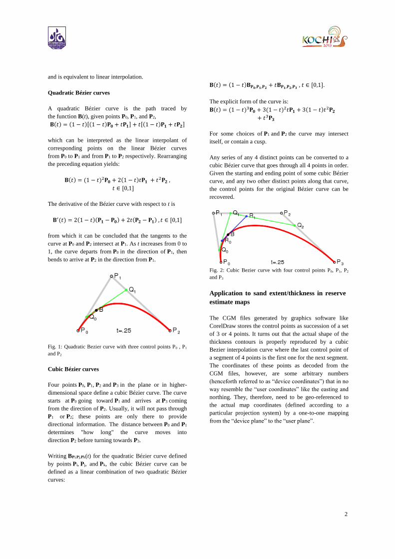
Quadratic Bézier curves

A quadratic Bézier curve is the path traced by

the function B(t), given points P0, P1, and P2,

𝐁(𝑡) = (1 − 𝑡)[(1 − 𝑡)𝐏𝟎 + 𝑡𝐏𝟏] + 𝑡[(1 − 𝑡)𝐏𝟏 + 𝑡𝐏𝟐]

which can be interpreted as the linear interpolant of

corresponding points on the linear Bézier curves

from P0 to P1 and from P1 to P2 respectively. Rearranging

the preceding equation yields:

𝐁(𝑡) = (1 − 𝑡)2𝐏𝟎 + 2(1 − 𝑡)𝑡𝐏𝟏 + 𝑡2𝐏𝟐 ,

𝑡 ∈ [0,1]

The derivative of the Bézier curve with respect to t is

𝐁′(𝑡) = 2(1 − 𝑡)(𝐏𝟏 − 𝐏𝟎) + 2𝑡(𝐏𝟐 − 𝐏𝟏) , 𝑡 ∈ [0,1]

from which it can be concluded that the tangents to the

curve at P0 and P2 intersect at P1. As t increases from 0 to

1, the curve departs from P0 in the direction of P1, then

bends to arrive at P2 in the direction from P1.

Fig. 1: Quadratic Bezier curve with three control points P0 , P1

and P2

Cubic Bézier curves

Four points P0, P1, P2 and P3 in the plane or in higher-

dimensional space define a cubic Bézier curve. The curve

starts at P0 going toward P1 and arrives at P3 coming

from the direction of P2. Usually, it will not pass through

P1 or P2; these points are only there to provide

directional information. The distance between P0 and P1

determines "how long" the curve moves into

direction P2 before turning towards P3.

Writing BPi,Pj,Pk(t) for the quadratic Bézier curve defined

by points Pi, Pj, and Pk, the cubic Bézier curve can be

defined as a linear combination of two quadratic Bézier

curves:

𝐁(𝑡) = (1 − 𝑡)𝐁𝐏𝟎,𝐏𝟏,𝐏𝟐+ 𝑡𝐁𝐏𝟏,𝐏𝟐,𝐏𝟑

, 𝑡 ∈ [0,1].

The explicit form of the curve is:

𝐁(𝑡) = (1 − 𝑡)3𝐏𝟎 + 3(1 − 𝑡)2𝑡𝐏𝟏 + 3(1 − 𝑡)𝑡2𝐏𝟐

+ 𝑡3𝐏𝟑

For some choices of P1 and P2 the curve may intersect

itself, or contain a cusp.

Any series of any 4 distinct points can be converted to a

cubic Bézier curve that goes through all 4 points in order.

Given the starting and ending point of some cubic Bézier

curve, and any two other distinct points along that curve,

the control points for the original Bézier curve can be

recovered.

Fig. 2: Cubic Bezier curve with four control points P0, P1, P2

and P3

Application to sand extent/thickness in reserve

estimate maps

The CGM files generated by graphics software like

CorelDraw stores the control points as succession of a set

of 3 or 4 points. It turns out that the actual shape of the

thickness contours is properly reproduced by a cubic

Bezier interpolation curve where the last control point of

a segment of 4 points is the first one for the next segment.

The coordinates of these points as decoded from the

CGM files, however, are some arbitrary numbers

(henceforth referred to as “device coordinates”) that in no

way resemble the “user coordinates” like the easting and

northing. They, therefore, need to be geo-referenced to

the actual map coordinates (defined according to a

particular projection system) by a one-to-one mapping

from the “device plane” to the “user plane”.

3

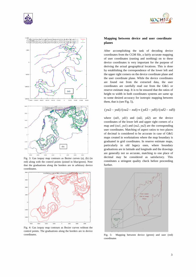
Fig. 3: Gas isopay map contours as Bezier curves (a), (b) (in

red) along with the control points (joined in blue/green). Note

that the graduations along the borders are in arbitrary device

coordinates.

Fig. 4: Gas isopay map contours as Bezier curves without the

control points. The graduations along the borders are in device

coordinates.

Mapping between device and user coordinate

planes

After accomplishing the task of decoding device

coordinates from the CGM file, a fairly accurate mapping

of user coordinates (easting and northing) on to these

device coordinates is very important for the purpose of

deriving the actual geographical locations. This is done

by establishing the correspondence of the lower left and

the upper right corners on the device coordinate plane and

the user coordinate plane. While the device coordinates

are found out from the extracted data, the user

coordinates are carefully read out from the G&G or

reserve estimate map. It is to be ensured that the ratios of

height to width in both coordinates systems are same up

to some desired accuracy for isotropic mapping between

them, that is (see Fig. 5),

)12/()12()12/()12( xdxdydydxuxuyuyu

where (xd1, yd1) and (xd2, yd2) are the device

coordinates of the lower left and upper right corners of a

map and (xu1, yu1) and (xu2, yu2) are the corresponding

user coordinates. Matching of aspect ratios to two places

of decimal is considered to be accurate in case of G&G

maps created in workstations where the map boundary is

graduated in grid coordinates. In reserve estimate maps,

particularly in old legacy ones, where boundary

graduations are in latitude and longitude and the drawings

are generally not so accurate, matching to one place of

decimal may be considered as satisfactory. This

constitutes a stringent quality check before proceeding

further.

Fig. 5: Mapping between device (green) and user (red)

coordinates

4

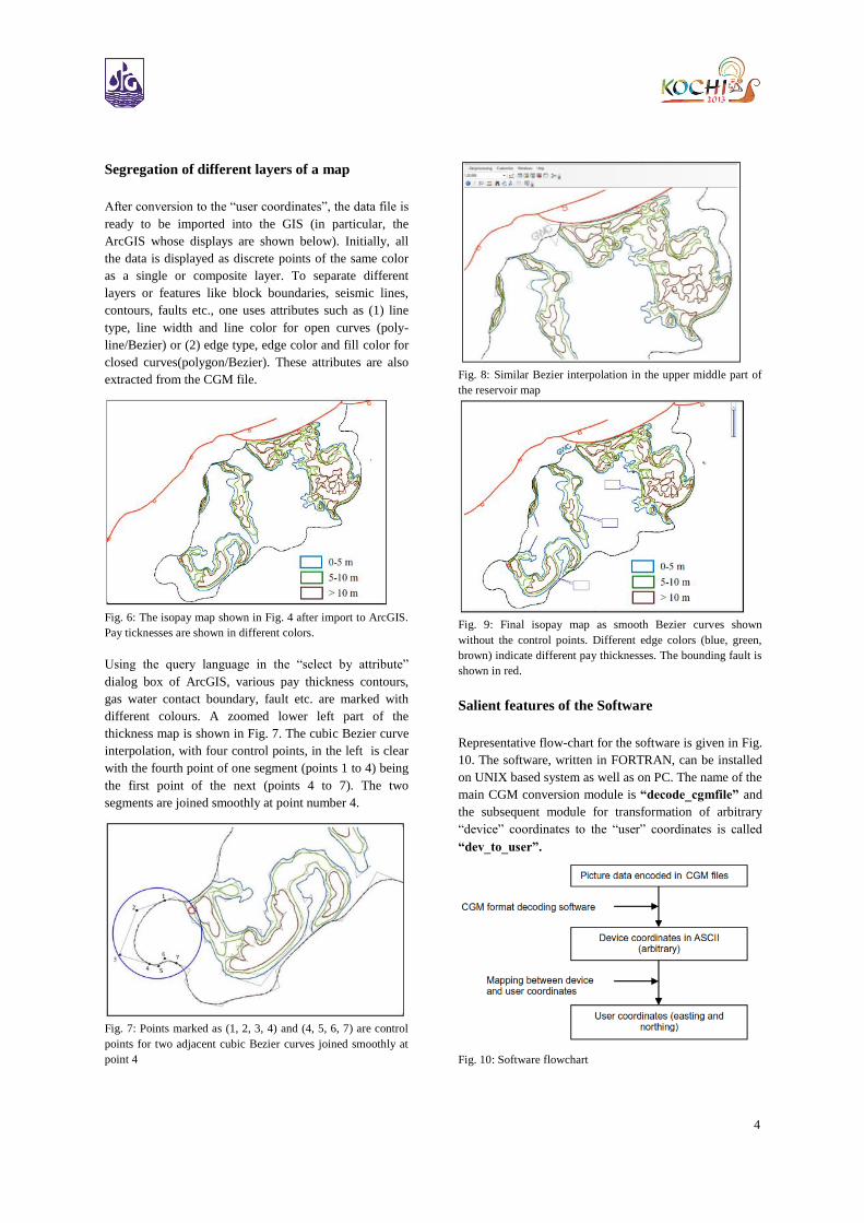
Segregation of different layers of a map

After conversion to the “user coordinates”, the data file is

ready to be imported into the GIS (in particular, the

ArcGIS whose displays are shown below). Initially, all

the data is displayed as discrete points of the same color

as a single or composite layer. To separate different

layers or features like block boundaries, seismic lines,

contours, faults etc., one uses attributes such as (1) line

type, line width and line color for open curves (poly-

line/Bezier) or (2) edge type, edge color and fill color for

closed curves(polygon/Bezier). These attributes are also

extracted from the CGM file.

Fig. 6: The isopay map shown in Fig. 4 after import to ArcGIS.

Pay ticknesses are shown in different colors.

Using the query language in the “select by attribute”

dialog box of ArcGIS, various pay thickness contours,

gas water contact boundary, fault etc. are marked with

different colours. A zoomed lower left part of the

thickness map is shown in Fig. 7. The cubic Bezier curve

interpolation, with four control points, in the left is clear

with the fourth point of one segment (points 1 to 4) being

the first point of the next (points 4 to 7). The two

segments are joined smoothly at point number 4.

Fig. 7: Points marked as (1, 2, 3, 4) and (4, 5, 6, 7) are control

points for two adjacent cubic Bezier curves joined smoothly at

point 4

Fig. 8: Similar Bezier interpolation in the upper middle part of

the reservoir map

Fig. 9: Final isopay map as smooth Bezier curves shown

without the control points. Different edge colors (blue, green,

brown) indicate different pay thicknesses. The bounding fault is

shown in red.

Salient features of the Software

Representative flow-chart for the software is given in Fig.

10. The software, written in FORTRAN, can be installed

on UNIX based system as well as on PC. The name of the

main CGM conversion module is “decode_cgmfile” and

the subsequent module for transformation of arbitrary

“device” coordinates to the “user” coordinates is called

“dev_to_user”.

Fig. 10: Software flowchart

5

From the study of a number of CGM files from different

sources, it has been found that the device coordinates

could be encoded in either of 2, 3 or 4 bytes and as any of

integers, fixed point real or floating point real numbers.

The module decode_cgmfile automatically detects this

and proceeds to convert the contents of the CGM file so

that the process is transparent to the user.

Conclusion and Remarks

In attempting to create a database of reservoir extent

maps drawn in graphics software like CorelDraw and

exported as CGM files, it was found that they are

encoded as a set of control points governing the shape of

the contours. These shapes are called Bezier curves which

are reconstructed by giving weights to the relative

positions of the control points as discussed in Section II.

These are very similar to the drawings that are generated

by choosing the “curve” option from available shapes in

preparing a powerpoint presentation.

Compare with the quartic(fourth order) Bézier curve

below.

The procedure to digitize reserve estimate maps also

include G&G interpretation maps at different depth and

time levels preserved as CGM files and store them in a

layered GIS-based database structure facilitating

corporate decision making.

Finally, it may be mentioned that the real utility of

creating a database is when any required information can

retrieved with ease. In the present case, all the archived

maps stored in ArcGIS as .shp files, can be quickly

imported back and superposed on any other maps on any

of the new generation interpretation workstation like

R5000, Petrel, Kingdom, whenever necessary. This will

enable the users to re-create the map features with

minimal effort.

Acknowledgement

The author wishes to express heartfelt gratitude to Mr.

A.K. Dwivedi, Ex-Basin Manager, Mr. A.V.Sathe, Basin

Manager and Mr. B.G. Samanta, General Manager (Geol)

of MBA Basin ONGC, Kolkata, where this work was

done.

Author is particularly indebted to Ms. Trishna Saha, Dy.

General Manager (Geol) who first prompted him to

include reservoir extent maps in his developed

methodology of creating GIS based database and gave the

first representative isopay data file that initiated this

work.

This work would not have been possible without the

initial encouragement of Mr. D.S. Mitra, GM(Geology)

and tremendous help extended by Mr. S. Majumdar of

Remote Sensing and Geomatics Lab, KDMIPE

Dehradun. The author is deeply indebted to them.