Bi-shifting Auto-Encoder for Unsupervised Domain Adaptation

Meina Kan1, Shiguang Shan1,2, Xilin Chen1

1Key Laboratory of Intelligent Information Processing of Chinese Academy of Sciences (CAS),

Institute of Computing Technology, CAS, Beijing, 100190, China2CAS Center for Excellence in Brain Science and Intelligence Technology

{kanmeina, sgshan, xlchen}@ict.ac.cn

Abstract

In many real-world applications, the domain of model

learning (referred as source domain) is usually inconsis-

tent with or even different from the domain of testing (re-

ferred as target domain), which makes the learnt model de-

generate in target domain, i.e., the test domain. To allevi-

ate the discrepancy between source and target domains, we

propose a domain adaptation method, named as Bi-shifting

Auto-Encoder network (BAE). The proposed BAE attempts

to shift source domain samples to target domain, and al-

so shift the target domain samples to source domain. The

non-linear transformation of BAE ensures the feasibility of

shifting between domains, and the distribution consisten-

cy between the shifted domain and the desirable domain is

constrained by sparse reconstruction between them. As a

result, the shifted source domain is supervised and follows

similar distribution as target domain. Therefore, any su-

pervised method can be applied on the shifted source do-

main to train a classifier for classification in target domain.

The proposed method is evaluated on three domain adap-

tation scenarios of face recognition, i.e., domain adapta-

tion across view angle, ethnicity, and imaging sensor, and

the promising results demonstrate that our proposed BAE

can shift samples between domains and thus effectively deal

with the domain discrepancy.

1. Introduction

For classification problems in computer vision, the most

typical technique is to learn a classifier on the training sam-

ples with class label and then apply it to classify the testing

samples. The basic assumption behind this is that the train-

ing samples and testing samples share the same or similar

distributions. However, in real world applications, many

factors (e.g., pose of faces, illumination, imaging quality,

etc) cause the mismatch of distribution between the training

samples and testing samples, which usually degenerate the

performance of learnt classifier on the testing samples.

The techniques for addressing this challenging domain

disparity problems are often referred as domain adaptation

[19][14][13][28][12] or generally as transfer learning [25].

Usually, the domain with labeled data, which is also where

the classifier is learnt, is called as source domain, and the

domain where the target task is conducted but with differ-

ent distribution is called as target domain. Rather than the

general transfer learning, this work only focuses on the do-

main adaption, in which the source domain and target do-

main share the same task but follow different distributions.

Depending on whether class labels are available for target

domain, domain adaptation can be categorized into two set-

tings [13][30][14], supervised domain adaptation and unsu-

pervised domain adaptation.

In scenario of supervised domain adaptation, labeled da-

ta is available in the target domain but the number is usually

too small to train a good classifier, while in unsupervised

domain adaptation only unlabeled data (but generally in

large-scale) is available in the target domain, which is more

challenging. This work mainly concentrates on the unsu-

pervised domain adaptation problem, of which the essence

is how to employ the unlabeled data of target domain to

guide the model learning from the labeled source domain.

An intuitive strategy is re-weighting or re-sampling the

samples of source domain to make the re-weighted/re-

sampled source domain shares similar distribution as target

domain, e.g., sample selection bias [38][18], and particular-

ly covariant shift [31][33][32][15][4], etc. These methods

usually need to measure the distance between two distribu-

tions, which is also very hard for complex scenarios.

More popular methods attempt to design domain-

invariant feature representation [2][5][24][23][30][26][14]

[13][10][12]. In [5], a structural correspondence learning

method automatically induces correspondences among fea-

tures from different domains with pivot feature, that be-

have in the same way for discriminative learning in both

domains. In Sampling Geodesic Flow (SGF) [14], a seri-

al of intermediate subspaces between the source and target

domains along the Grassmann manifold are sampled to de-

3846

scribe the underlying domain shift, and the projections of la-

beled source domain data onto these subspaces can be used

to learn a classifier applicable for the target domain. Fur-

thermore, in [13], a Geodesic Flow Kernel (GFK) approach

is proposed to characterize the domain shift by integrating

an infinite number of subspaces. In [12], a subset of la-

beled instances in source domain that are similar to the tar-

get domain is identified as landmarks to bridge the source

and target domains by constructing an easier auxiliary do-

main adaptation task. Based on domain-invariant feature,

the learnt model or metric from labeled source domain can

be applicable for the classification in target domain.

On the other hand, some methods endeavor to directly

optimize a classifier or metric which follows small or no

discrepancy with the target domain [8][6][30][27]. In [7],

a progressive transductive support vector machine is devel-

oped to iteratively label and modify the unlabeled target do-

main to achieve a wider margin for target domain. In [6],

the discriminant classifier is adjusted step by step to the tar-

get domain by iteratively deleting the samples from source

domain and adding samples from target domain until the fi-

nal classification function is determined only based on sam-

ples from target domain. Most of these methods exploit an

iteration scheme to gradually adapt the supervised informa-

tion of the source domain to the target domain. In [30], the

domain-invariant feature and classifier are jointly learnt by

optimizing an information-theoretic metric as an proxy to

the expected misclassification error on the target domain.

For the existing methods, maximum mean discrepan-

cy, K-L and Bregman divergence are the most common-

ly used criteria to measure the discrepancy between source

and target domains. Recently, low-rank representation con-

straint is proposed to guide the reduction of discrepancy

between domains. In [20], the samples of source domain

are mapped into an intermediate representation such that

the transformed source domain samples can be linearly re-

constructed by target domain samples in lowest rank struc-

ture, and then the transformed source samples can be used

to learn a classifier for classification in target domain. In

[28][29], a common and discriminant subspace is achieved

via a low-rank representation constraint, which attempts to

ensure that each datum in source domain can be linearly

represented by target domain samples. In [21], the samples

in source domain are transformed to target domain where

each source domain sample can be linearly reconstructed by

sparse number of target domain samples. In [11], a high lev-

el feature representation is learnt as domain-invariant fea-

ture by employing denoising auto-encoder to recover the in-

put instances from both source and target domains, which is

expected to characterize the commonality of both domains.

In works [20][28][29], linear transformation is employed

to project source domain, target domain or both to a sub-

space where the samples of one domain can be linearly

Figure 1. An overview of Bi-shifting Auto-Encoder (BAE).

Through BAE, a source domain sample can be transformed to tar-

get domain where it can be sparsely and linearly reconstructed by

target domain samples, and a target domain sample can be trans-

formed to source domain where it can be sparsely and linearly

reconstructed by source domain samples too.

reconstructed by another domain. The linear reconstruc-

tion principle enforces the domain consistency and achieves

promising performance. However in many cases the source

domain might be quite different from the target domain,

and linear transformation can hardly remove the discrep-

ancy completely for further linear reconstruction. The work

[11] employs non-linear transformation to model the vari-

ations but with no domain consistency constraint, and thus

cannot well characterize the commonality of domains. In

order to effectively handle the domain discrepancy, we pro-

pose a Bi-shifting Auto-Encoder network (BAE) which can

shift source domain samples to target domain and also shift

the target domain samples to source domain, as shown in

Fig. 1. In BAE, the non-linear transformation ensures the

feasibility of shifting between domains, and the sparse re-

construction ensures the distribution consistency between

the shifted domain and desirable domain. Specifically, our

bi-shifting auto-encoder network has one common encoder

fc, two decoders fs and ft which can map an image to the

source and target domain respectively. As a result, the

source domain can be shifted to target domain along with

its class label, and any supervised method can be applied

on shifted source domain to train a classifier for classifica-

tion in target domain, as the shifted source domain follows

similar distribution as target domain.

The reminder of this paper is organized as follows. Sec.

3847

2 presents the proposed bi-shifting auto-encoder network

and its optimization. Sec. 3 evaluates the proposed method

on three domain adaptation face recognition scenarios, i.e.,

domain adaptation across view angle, ethnicity and imaging

sensor. Finally, a conclusion is given in the last section.

2. Bi-shifting Auto-Encoder

2.1. Notations and Problem

For clear description in the following, we first define

some notations. In the whole text, upper-case and lower-

case characters represent the matrices and vectors respec-

tively. Unless otherwise specified, the symbols s and t used

in the superscript or subscript denotes the source domain

and target domain respectively.

In source domain, there are ns labeled samples in d-

dimension, denoted as Xs = [xs1,x

s2, · · · ,x

sns] ∈ R

d×ns ,

with their class labels ys = [ys1, ys2, · · · , y

sns], ysi ∈

{1, 2, · · · , cs}, where xsi ∈ R

d×1 is the feature represen-

tation of the i-th source domain sample, ysi is its class label,

and cs is the number of classes in the source domain.

In target domain, there are nt samples in d-dimension

without class label, denoted as Xt = [xt1,x

t2, · · · ,x

tnt] ∈

Rd×nt , where xt

i ∈ Rd×1 is the feature representation of

the i-th target domain sample.

The problem to deal with is how to learn a model for

classification in target domain with only unlabeled samples

of target domain Xt and labeled but distributed differently

samples of source domain (Xs,ys).

2.2. Auto­Encoder (AE)

For an auto-encoder neural network [3][35] with single

hidden layer, it is usually compromised of two parts, en-

coder and decoder. The encoder, denoted as f , attempts to

map the input x∈Rd×1 into hidden representations, denoted

as z∈Rr×1, in which r is the number of neurons in hidden

layer. Typically, f is a nonlinear transform as follows:

z = f(x) = s(Wx+ b), (1)

where W ∈ Rr×d is a linear transform , b ∈ R

r×1 is

the basis and s(·) is the so-called element-wise “activa-

tion function”, which is usually non-linear, such as sigmoid

function s(x) = 1

1+e−x or tanh function s(x) = ex−e−x

ex+e−x .

The decoder, denoted as g, tries to map the hidden rep-

resentation z back to the input x, i.e.,

x = g(z) = s(W′z+ b′), (2)

withW′ ∈ Rd×r and basis b′ ∈ R

d×1.

To optimize the parameters W,b, W′ and b′, usually

the least square error is employed as the cost function:

minW,b,W′,b′

∑N

i=1‖xi−g(f(xi))‖

22, (3)

where xi represents the ith one of N training sample. Due

to the non-linearity of encoder and decoder in Eq. (3), it is

difficult to solve, and thus the gradient descent algorithm is

commonly employed.

2.3. Bi­shifting Auto­Encoder (BAE)

The typical auto-encoder in Eq. (3) tries to reconstruc-

t the input itself, which is usually employed for dimension

reduction, or feature learning. Nevertheless, our proposed

bi-shifting auto-encoder network attempts to shift samples

between domains to deal with the domain discrepancy. As

shown in Fig. 1, our bi-shifting auto-encoder network con-

sists of one encoder fc, and two decoders, i.e., gs and gt,

which can transform an input sample to source domain and

target domain respectively.

Specifically, the encoder fc aims to map an input sample

x into hidden feature representation z which is common to

both source and target domains as below:

z , fc(x) = σ(Wcx+ bc) (4)

The decoder gs intends to map the hidden representation to

source domain, and decoder gt intends to map the hidden

representation to target domain as follows:

gs(z) = σ(Wsz+ bs),

gt(z) = σ(Wtz+ bt),(5)

where s(·) is the element-wise nonlinear activation func-

tion, e.g., sigmoid or tanh function, Wc and bc are the pa-

rameters for encoder fc, Ws and bs are the parameters for

decoder gs, Wt and bt are the parameters for decoder gt.

For source domain Xs, on one hand, with encoder fc and

decoder gs they should be mapped to source domain, i.e.,

Xs itself. On the other hand, with encoder fc and decoder

gt, they should be mapped to target domain. Although it

is unknown what the mapped samples look like, they are

expected to follow the same distribution as target domain.

This kind of distribution consistency between two domains

can be characterized by the local structure consistency.

The two domains Xs and Xt can be generally considered

to lie on two manifolds Ms and Mt, and the distance be-

tween the two manifolds can be used to describe the domain

discrepancy of them. As indicated in [36], the distance be-

tween manifolds can be measured by the distance between

instances of both manifolds. Given the instances xsi |

ns

i=1

from Ms, assume that we can traverse all samplings of ns

instances from Mt, then we can get a sampling xt∗i |ns

i=1that

minimize the distance of∑ns

i=1||xs

i − xt∗i ||2, which can be

used to depict the distance of the two manifolds. Howev-

er, actually it is impossible to look through all samplings to

get the optimal xt∗i |ns

i=1. But we have another sampling Xt

sampled from the same manifold as xt∗i |ns

i=1. This mean-

s that each xt∗i can be reconstructed by using its several

3848

neighbors from Xt, i.e., xt∗i =

∑r

k=1bkx

tik with xt

ik as

one of the r neighbors. xt∗i =

∑r

k=1bkx

tik can be fur-

ther formulated as xt∗i = Xtβ

ti , and βt

i is a sparse vector

with the non-zero values corresponding to the local neigh-

bors. Consequently,∑ns

i=1||xs

i − Xtβti ||

2 can be used to

describe the distance between the two domains, where βti

should be locally sparse. For simplicity, we relax βti to be

sparse without explicit restriction of the locality, since the

non-zeros values from sparsity usually tends to be local.

As shown in Fig. 2, to enforce the shifted source domain

and target domain share similar distribution, each mapped

source domain sample should be sparely reconstructed by

several neighbors from target domain, formulated as below:

gt(fc(xsi )) = Xtβ

ti , s.t., |βt

i |0 < τ, (6)

where βti is the sparse coefficients for the reconstruction of

shifted source domain sample. Eq. (6) enforces that each

local structure of shifted source domain is consistent with

that of target domain, which ensures that the shifted source

domain follow similar distribution as target domain. The

overall objective for the samples of source domain Xs can

be formulated as below, with Bt =[βt1, · · · ,β

tns

]:

minfc,gs,gt,β

t

i

||Xs−gs(fc(Xs))||22+||XtBt−gt(fc(Xs))||

22

s.t., |βti |0 < τ,

(7)

Here, the gs(fc(Xs)) and gt(fc(Xs)) represent the ma-

trices of [gs(fc(xs1)),gs(fc(x

s2)), · · · ,gs(fc(x

sns))] and

[gt(fc(xs1)),gt(fc(x

s2)), · · · ,gt(fc(x

sns))] respectively for

concise representation. The same simplifications are used

hereinafter if without misunderstanding.

Similarly, for the samples of target domain Xt, on

one hand, with encoder fc and decoder gt they should be

mapped to the target domain, i.e., Xt itself. On the oth-

er hand, with encoder fc and decoder gs they should be

mapped to the source domain, where they are constrained to

be sparsely reconstructed by several neighbors from source

domain, so as to ensure a similar distribution between the

source domain and shifted target domain. The overall ob-

jective for the samples of target domain Xt can be formu-

lated as below with Bs =[βs1, · · · ,β

snt

]:

minfc,gs,gt,β

s

i

||XsBs−gs(fc(Xt))||22+||Xt−gt(fc(Xt))||

22

s.t., |βsi |0 < τ,

(8)

The L0-norm problem in Eq. (7) and Eq. (8) are non-

convex and hard to solve, so they are relaxed to L1-norm as

most existing methods do. Therefore, the objective of the

bi-shifting auto-encoder can be formulated as following:

minfc,gs,gt,Bs,Bt

||Xs−gs(fc(Xs))||22+ ||XtBt−gt(fc(Xs))||

22

+ ||XsBs−gs(fc(Xt))||22+||Xt−gt(fc(Xt))||

22

+ γ(∑ns

i=1|βt

i |1 +∑nt

i=1|βs

i |1

).

(9)

source domain sample

target domain sampleshifted source domain sample

bi-shifting AE (BAE)

shifted target domain sample

Figure 2. Illustration of sparse reconstruction constraint for distri-

bution consistency. If each shifted source domain sample (green

triangle) can be sparsely reconstructed by several local neighbors

from target domain (green circle), they tends to follow similar lo-

cal structure, meaning similar distribution in whole. Similarly,

each shifted target domain sample (yellow circle) is constrained

to be sparsely reconstructed by source domain neighbors (yellow

triangle), to enforce them follow similar distributions.

Here, γ is a parameter to control the sparsity, i.e., a larger

γ leads to less samples selected for the sparse reconstruc-

tion, and smaller γ leads to more samples selected for the

sparse reconstruction. Empirically, the first four terms need

to be normalized to similar scale to avoid the dominance of

some terms. In Eq. (9), the nonlinear mapping function of

the encoder and decoders ensures the feasibility of shifting

samples from one domain to another, while the sparse re-

construction constraint promises the shifted domain follows

similar distribution as the desirable domain.

With Eq. (9), a bi-shifting auto-encoder can be achieved

to map any input sample to source and target domains re-

spectively. Especially, the labeled source domain samples,

(Xs,ys), can be shifted to target domain along with its class

label as (Gt,ys), Gt , gt(fc(Xs)). The mapped source

domain samples Gt share similar distribution as target do-

main, so any supervised method can be applied to learn a

classifier for classification in target domain. In this work,

Fisher Linear discriminant analysis (LDA) [1] is employed

for supervised dimension reduction and the nearest neigh-

bor classifier for recognition.

2.4. Optimization

Eq. (9) is hard to solve due to the complex non-linearity

of the encoder and decoder, so the alternating optimiza-

tion approach is employed to iteratively solve the network

fc,gs,gt and sparse reconstruction coefficients Bs,Bt.

STEP 1: given fc,gs and gt, optimize Bs and Bt.

When fc,gs and gt are fixed, the objective in Eq. (9) can

3849

be reformulated as below:

minBs,Bt

||XtBt −Gt||22 + ||XsBs −Gs||

22

+γ(∑ns

i=1|βt

i |1 +∑nt

i=1|βs

i |1

) (10)

with gt(fc(Xs)) , Gt =[gt1, · · · ,g

tns

]and gs(fc(Xt)) ,

Gs =[gs1, · · · ,g

snt

]. In Eq. (10), Bs and Bt are indepen-

dent of each other, so they can be optimized independently.

Namely, Bs =[βs1, · · · ,β

snt

]can be optimized as:

minβs

i

||XsBs −Gs||22 + γ

∑nt

i=1|βs

i |1

⇔ minβs

i

∑nt

i=1||Xsβ

si − gs

i ||22 + γ

∑nt

i=1|βs

i |1(11)

As seen, βs1, β

s2, · · · ,β

snt

in Eq. (11) are also independent

of each other, which means each βsi can be further separate-

ly solved as a lasso problem:

minβs

i||Xsβ

si − gs

i ||22 + γ|βs

i |1 (12)

Eq. (12) can be easily solved by using forward stepwise

regression like algorithm, i.e., the least angle regression [9].

Similarly, each βti in Bt is also independent of each oth-

er and can be separately optimized as below:

minβt

i

||Xtβti − gt

i ||22 + γ|βt

i |1. (13)

The problem in Eq. (13) can be also easily solved by using

the least angle regression algorithm [9].

STEP 2: given Bs and Bt, optimize fc,gs and gt.

When Bs and Bt are fixed, the objective in Eq. (9) can

be reformulated as below:

minfc,gs,gt

||Xs − gs(fc(Xs))||22 + ||Xt − gt(fc(Xs))||

22

+ ||Xs − gs(fc(Xt))||22 + ||Xt − gt(fc(Xt))||

22

(14)

with XtBt , Xt and XsBs , Xs. Eq. (14) can be easily

optimized by gradient descent as the typical auto-encoder.

STEP 3: Repeat step 1 and 2 until fc,gs,gt,Bs and Bt

converge or a maximum number of iterations is exceeded.

Before the alternation, the network fc, gs and gt are ini-

tialized by optimizing the following objective:

minfc,gs,gt,Bs,Bt

||Xs−gs(fc(Xs))||22+||Xt−gt(fc(Xt))||

22 (15)

3. Experiments

In this section, we evaluate the proposed method by com-

paring with existing methods on three face recognition sce-

narios: 1) domain adaptation across view angle, where the

source and target domains are from different view angles;

2) domain adaptation across ethnicity, where the source

and target domains are from different ethnicities, Mongo-

lian and Caucasian; 3) domain adaptation across imaging

sensor, where the images in source and target domains are

captured under two different sensors, visual light (VIS) and

near-infrared light (NIR) sensors. Several competitive ap-

proaches are briefly described as below. For all method-

s, their parameters are tuned to report the best results, and

Linear Discriminant Analysis (LDA) is employed for super-

vised learning or initialization for fair comparison.

PCA [34]. Principal Component Analysis is a typical

unsupervised method, taken as the baseline by being direct-

ly conducted on target domain.

Source LDA [1]. Fisher’s Linear Discriminant analysis

is a widely-used supervised approach for feature extraction.

The LDA trained on the source domain with no adaptation

is also tested as a baseline, denoted as “Source LDA”.

ITL [30]. Information Theoretical Learning aims at i-

dentifying a discriminative subspace where source and tar-

get domains are similarly distributed, by optimizing an in-

formation theoretic metric as an proxy to the expected mis-

classification error on target domain. ITL is initialized with

random matrix, PCA and LDA respectively, and dimension

of the metric is tuned so as to report the best performance.

SGF [14]. In Sampling Geodesic Flow approach, a se-

ries of intermediate common representations are created

by projecting the data onto the sampled intermediate sub-

spaces. With the projected intermediate representation, L-

DA and 1-NN classifier is employed for classification. The

number of sampled subspaces, dimension of subspace, and

the dimension of LDA are tuned to report the best results.

GFK [14]. Geodesic Flow Kernel models domain shift

by integrating an infinite number of subspaces that charac-

terize changes in geometric and statistical properties from

the source to target domain. For GFK, the supervised LDA

subspace is used as the source subspace, PCA subspace is

used as the target subspace, and 1-NN classifier is employed

for final classification. The dimension of source subspace

and target subspace are tuned to report the best results.

Landmarks [12]. This approach automatically discov-

Figure 3. Performance of the proposed BAE w.r.t. different num-

ber of hidden neurons and different sparsity γ, with Caucasian as

source domain and Mongolian as target domain respectively.

3850

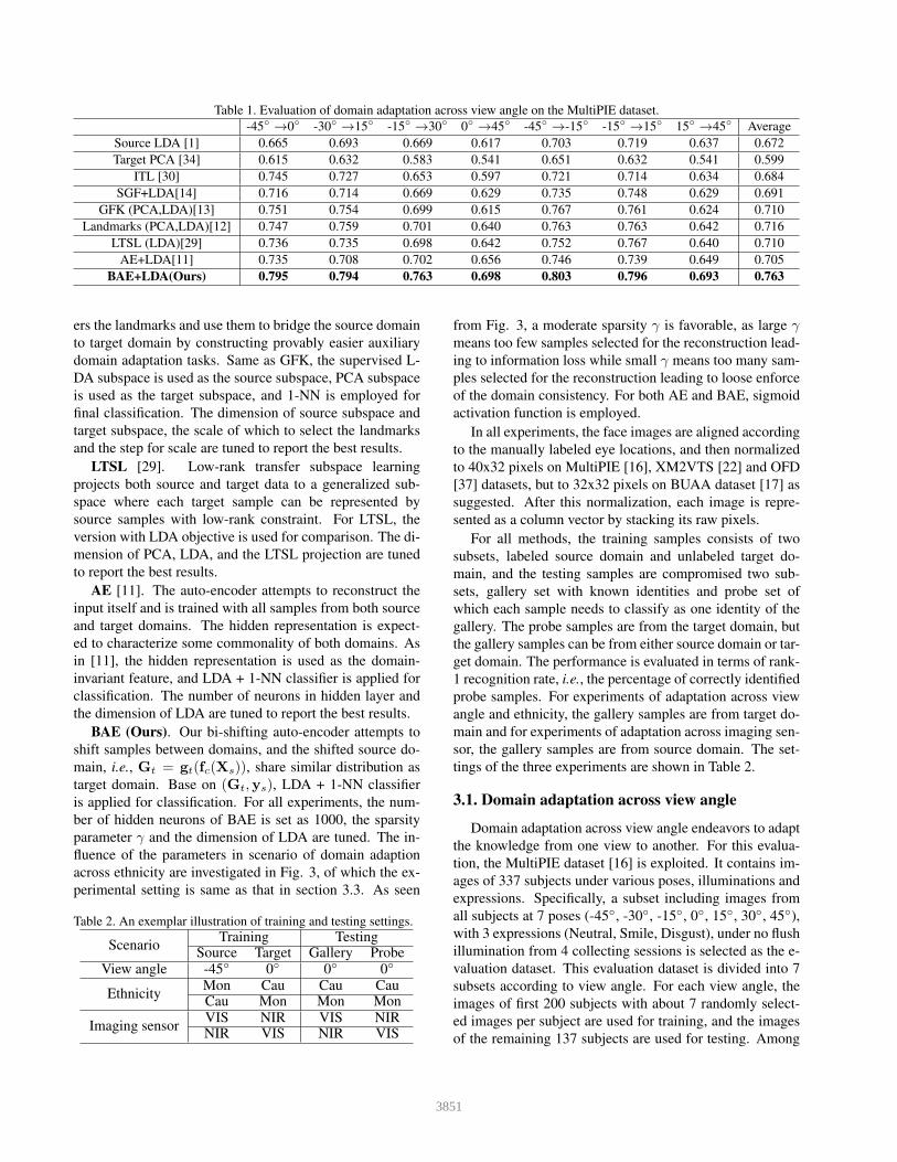
Table 1. Evaluation of domain adaptation across view angle on the MultiPIE dataset.

-45◦ →0◦ -30◦ →15◦ -15◦ →30◦ 0◦ →45◦ -45◦ →-15◦ -15◦ →15◦ 15◦ →45◦ Average

Source LDA [1] 0.665 0.693 0.669 0.617 0.703 0.719 0.637 0.672

Target PCA [34] 0.615 0.632 0.583 0.541 0.651 0.632 0.541 0.599

ITL [30] 0.745 0.727 0.653 0.597 0.721 0.714 0.634 0.684

SGF+LDA[14] 0.716 0.714 0.669 0.629 0.735 0.748 0.629 0.691

GFK (PCA,LDA)[13] 0.751 0.754 0.699 0.615 0.767 0.761 0.624 0.710

Landmarks (PCA,LDA)[12] 0.747 0.759 0.701 0.640 0.763 0.763 0.642 0.716

LTSL (LDA)[29] 0.736 0.735 0.698 0.642 0.752 0.767 0.640 0.710

AE+LDA[11] 0.735 0.708 0.702 0.656 0.746 0.739 0.649 0.705

BAE+LDA(Ours) 0.795 0.794 0.763 0.698 0.803 0.796 0.693 0.763

ers the landmarks and use them to bridge the source domain

to target domain by constructing provably easier auxiliary

domain adaptation tasks. Same as GFK, the supervised L-

DA subspace is used as the source subspace, PCA subspace

is used as the target subspace, and 1-NN is employed for

final classification. The dimension of source subspace and

target subspace, the scale of which to select the landmarks

and the step for scale are tuned to report the best results.

LTSL [29]. Low-rank transfer subspace learning

projects both source and target data to a generalized sub-

space where each target sample can be represented by

source samples with low-rank constraint. For LTSL, the

version with LDA objective is used for comparison. The di-

mension of PCA, LDA, and the LTSL projection are tuned

to report the best results.

AE [11]. The auto-encoder attempts to reconstruct the

input itself and is trained with all samples from both source

and target domains. The hidden representation is expect-

ed to characterize some commonality of both domains. As

in [11], the hidden representation is used as the domain-

invariant feature, and LDA + 1-NN classifier is applied for

classification. The number of neurons in hidden layer and

the dimension of LDA are tuned to report the best results.

BAE (Ours). Our bi-shifting auto-encoder attempts to

shift samples between domains, and the shifted source do-

main, i.e., Gt = gt(fc(Xs)), share similar distribution as

target domain. Base on (Gt,ys), LDA + 1-NN classifier

is applied for classification. For all experiments, the num-

ber of hidden neurons of BAE is set as 1000, the sparsity

parameter γ and the dimension of LDA are tuned. The in-

fluence of the parameters in scenario of domain adaption

across ethnicity are investigated in Fig. 3, of which the ex-

perimental setting is same as that in section 3.3. As seen

Table 2. An exemplar illustration of training and testing settings.

ScenarioTraining Testing

Source Target Gallery ProbeView angle -45◦ 0◦ 0◦ 0◦

EthnicityMon Cau Cau CauCau Mon Mon Mon

Imaging sensorVIS NIR VIS NIRNIR VIS NIR VIS

from Fig. 3, a moderate sparsity γ is favorable, as large γ

means too few samples selected for the reconstruction lead-

ing to information loss while small γ means too many sam-

ples selected for the reconstruction leading to loose enforce

of the domain consistency. For both AE and BAE, sigmoid

activation function is employed.

In all experiments, the face images are aligned according

to the manually labeled eye locations, and then normalized

to 40x32 pixels on MultiPIE [16], XM2VTS [22] and OFD

[37] datasets, but to 32x32 pixels on BUAA dataset [17] as

suggested. After this normalization, each image is repre-

sented as a column vector by stacking its raw pixels.

For all methods, the training samples consists of two

subsets, labeled source domain and unlabeled target do-

main, and the testing samples are compromised two sub-

sets, gallery set with known identities and probe set of

which each sample needs to classify as one identity of the

gallery. The probe samples are from the target domain, but

the gallery samples can be from either source domain or tar-

get domain. The performance is evaluated in terms of rank-

1 recognition rate, i.e., the percentage of correctly identified

probe samples. For experiments of adaptation across view

angle and ethnicity, the gallery samples are from target do-

main and for experiments of adaptation across imaging sen-

sor, the gallery samples are from source domain. The set-

tings of the three experiments are shown in Table 2.

3.1. Domain adaptation across view angle

Domain adaptation across view angle endeavors to adapt

the knowledge from one view to another. For this evalua-

tion, the MultiPIE dataset [16] is exploited. It contains im-

ages of 337 subjects under various poses, illuminations and

expressions. Specifically, a subset including images from

all subjects at 7 poses (-45◦, -30◦, -15◦, 0◦, 15◦, 30◦, 45◦),

with 3 expressions (Neutral, Smile, Disgust), under no flush

illumination from 4 collecting sessions is selected as the e-

valuation dataset. This evaluation dataset is divided into 7

subsets according to view angle. For each view angle, the

images of first 200 subjects with about 7 randomly select-

ed images per subject are used for training, and the images

of the remaining 137 subjects are used for testing. Among

3851

Table 3. Evaluation of domain adaptation across ethnicity.

Cau→Mon Mon→Cau Average

Source LDA [1] 0.679 0.676 0.678

ITL [30] 0.801 0.775 0.788

SGF+LDA[14] 0.790 0.751 0.771

GFK (PCA,LDA)[13] 0.738 0.721 0.730

Landmarks (PCA,LDA)[12] 0.718 0.763 0.741

LTSL (LDA)[29] 0.791 0.793 0.792

AE+LDA[11] 0.784 0.786 0.785

BAE+LDA(Ours) 0.892 0.826 0.859

the testing images, 1 and 4 images per subject are random-

ly selected as the gallery and probe images respectively. In

summary, for each view angle, 1,383 images from 200 sub-

jects are used as the training set, 137 images from the rest

137 subjects are used as gallery, and 553 images from 137

subjects are used as probes. For each evaluation, the train-

ing set with class label from a source view and the training

set without label from a target view are used for training, the

gallery and probe sets from target view are used for testing.

The evaluation results are shown in Table 1. As seen

from these comparisons, PCA and Source LDA perform-

s the worst as no supervised information or no adaptation

is employed. As expected, the domain adaptation meth-

ods, e.g., SGF and ITL, achieve much better performance

as they exploit the knowledge from both source and target

domain via common subspace or domain-invariant feature

representation. Furthermore, the GFK and Landmarks out-

perform SGF, benefited from integrating an infinite number

of subspaces. Although LTSL is a linear method, it also

performs promising benefited from the low-rank constraint.

The Auto-Encoder methods performs better than Source L-

DA, but slightly worse than GFK, Landmarks and LTSL, as

it does not reduce the domain disparity explicitly and thus

can not promise a discriminative commonality. Compared

with these method, our BAE performs the best with an im-

provement up to 4.7% on average, as the non-linearity of

auto-encoder coupled with sparse representation constrain-

t can ensure that the shifted source domain follow similar

distribution as target domain. The distribution of different

layers of BAE is shown in Fig. 4 and some shifted source

domain samples can be found in Fig. 5.

3.2. Domain adaptation across ethnicity

In many cases, the training samples are from one ethnic-

ity, but the testing samples to classify are from another eth-

nicity. To explore domain adaptation across ethnicity, the

XM2VTS dataset [22] consisting of mainly Caucasian and

the Oriented Face Dataset (OFD) [37] consisting of mainly

Mongolian are used. The XM2VTS dataset contains 3,440

images of 295 subjects taken over a period of four months

with different pose and illumination variations. Eight im-

ages with slight pose variation per subject are randomly se-

Table 4. Evaluation of domain adaptation across imaging sensor.

VIS→NIR NIR→VIS Average

Source LDA [1] 0.816 0.779 0.798

ITL [30] 0.858 0.877 0.868

SGF+LDA[14] 0.841 0.832 0.837

GFK (PCA,LDA)[13] 0.850 0.867 0.859

Landmarks (PCA,LDA)[12] 0.859 0.871 0.865

LTSL (LDA)[29] 0.868 0.878 0.873

AE+LDA[11] 0.827 0.846 0.837

BAE+LDA(Ours) 0.904 0.920 0.912

lected for evaluation. Specifically, for each subject, 4 of the

8 images are randomly selected to form the training set, and

the remaining images form the testing set: for each subjec-

t, 1 image is enrolled into gallery and the left 3 are used as

probes. For OFD dataset, a subset consisting of 800 subject-

s with 4 images per subject under slight lighting variations

are used. The images of the first 400 subjects are used as

training data, and images of the rest 400 subjects are used

for testing. Specifically, 1 image per subject is randomly

selected to form the gallery, and the rest 3 images of each

subject are used as the probes.

In summary, for XM2VTS, 1,180 images from 295 sub-

jects are used as training data, 295 images from 295 subjects

are used as gallery, and 885 images from 295 subjects are

used as probe. For OFD, 1,600 images from 400 subject-

s are used as training data, 400 images from 400 subject-

s (one per subject) are used as gallery, and 1,200 images

from 400 subjects are used as probes. For both datasets, if

one is used as source domain, the training set of this dataset

is used along with class label; if the dataset is used as the

target domain, the training set is used without class label,

the gallery and probe set are used for testing.

The evaluation results are shown in Table 3. As seen,

Source LDA performs the worst, SGF, GFK, AE, and Land-

marks perform much better as expected. Besides, ITL and

LTSL perform even better and the reason we guess is that

the discrepancy caused by ethnicity is smaller than view an-

gle which is easier to handle by linear model. Our BAE

can further improve the performance up to 5.9% compared

with the best performer LTSL. This demonstrates that the

discrepancy between the shifted source domain from our

BAE and target domain is smaller than that of those domain-

Figure 4. The distribution of the first two dimensions from Princi-

pal Component Analysis (PCA) projections of input layer, hidden

layer, and output layer of BAE on MultiPIE (-30◦ →15◦).

3852

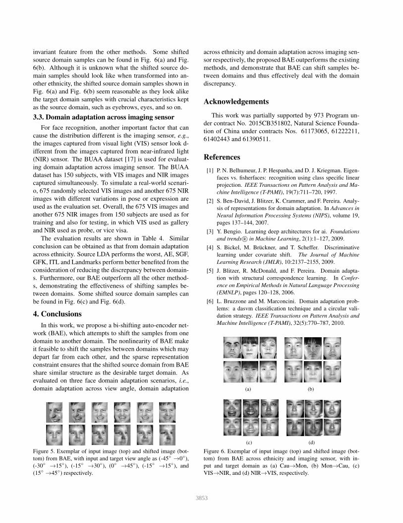
invariant feature from the other methods. Some shifted

source domain samples can be found in Fig. 6(a) and Fig.

6(b). Although it is unknown what the shifted source do-

main samples should look like when transformed into an-

other ethnicity, the shifted source domain samples shown in

Fig. 6(a) and Fig. 6(b) seem reasonable as they look alike

the target domain samples with crucial characteristics kept

as the source domain, such as eyebrows, eyes, and so on.

3.3. Domain adaptation across imaging sensor

For face recognition, another important factor that can

cause the distribution different is the imaging sensor, e.g.,

the images captured from visual light (VIS) sensor look d-

ifferent from the images captured from near-infrared light

(NIR) sensor. The BUAA dataset [17] is used for evaluat-

ing domain adaptation across imaging sensor. The BUAA

dataset has 150 subjects, with VIS images and NIR images

captured simultaneously. To simulate a real-world scenari-

o, 675 randomly selected VIS images and another 675 NIR

images with different variations in pose or expression are

used as the evaluation set. Overall, the 675 VIS images and

another 675 NIR images from 150 subjects are used as for

training and also for testing, in which VIS used as gallery

and NIR used as probe, or vice visa.

The evaluation results are shown in Table 4. Similar

conclusion can be obtained as that from domain adaptation

across ethnicity. Source LDA performs the worst, AE, SGF,

GFK, ITL and Landmarks perform better benefited from the

consideration of reducing the discrepancy between domain-

s. Furthermore, our BAE outperform all the other method-

s, demonstrating the effectiveness of shifting samples be-

tween domains. Some shifted source domain samples can

be found in Fig. 6(c) and Fig. 6(d).

4. Conclusions

In this work, we propose a bi-shifting auto-encoder net-

work (BAE), which attempts to shift the samples from one

domain to another domain. The nonlinearity of BAE make

it feasible to shift the samples between domains which may

depart far from each other, and the sparse representation

constraint ensures that the shifted source domain from BAE

share similar structure as the desirable target domain. As

evaluated on three face domain adaptation scenarios, i.e.,

domain adaptation across view angle, domain adaptation

Figure 5. Exemplar of input image (top) and shifted image (bot-

tom) from BAE, with input and target view angle as (-45◦ →0◦),

(-30◦ →15◦), (-15◦ →30◦), (0◦ →45◦), (-15◦ →15◦), and

(15◦ →45◦) respectively.

across ethnicity and domain adaptation across imaging sen-

sor respectively, the proposed BAE outperforms the existing

methods, and demonstrate that BAE can shift samples be-

tween domains and thus effectively deal with the domain

discrepancy.

Acknowledgements

This work was partially supported by 973 Program un-

der contract No. 2015CB351802, Natural Science Founda-

tion of China under contracts Nos. 61173065, 61222211,

61402443 and 61390511.

References

[1] P. N. Belhumeur, J. P. Hespanha, and D. J. Kriegman. Eigen-

faces vs. fisherfaces: recognition using class specific linear

projection. IEEE Transactions on Pattern Analysis and Ma-

chine Intelligence (T-PAMI), 19(7):711–720, 1997.

[2] S. Ben-David, J. Blitzer, K. Crammer, and F. Pereira. Analy-

sis of representations for domain adaptation. In Advances in

Neural Information Processing Systems (NIPS), volume 19,

pages 137–144, 2007.

[3] Y. Bengio. Learning deep architectures for ai. Foundations

and trends R© in Machine Learning, 2(1):1–127, 2009.

[4] S. Bickel, M. Bruckner, and T. Scheffer. Discriminative

learning under covariate shift. The Journal of Machine

Learning Research (JMLR), 10:2137–2155, 2009.

[5] J. Blitzer, R. McDonald, and F. Pereira. Domain adapta-

tion with structural correspondence learning. In Confer-

ence on Empirical Methods in Natural Language Processing

(EMNLP), pages 120–128, 2006.

[6] L. Bruzzone and M. Marconcini. Domain adaptation prob-

lems: a dasvm classification technique and a circular vali-

dation strategy. IEEE Transactions on Pattern Analysis and

Machine Intelligence (T-PAMI), 32(5):770–787, 2010.

(a) (b)

(c) (d)

Figure 6. Exemplar of input image (top) and shifted image (bot-

tom) from BAE across ethnicity and imaging sensor, with in-

put and target domain as (a) Cau→Mon, (b) Mon→Cau, (c)

VIS→NIR, and (d) NIR→VIS, respectively.

3853

[7] Y. Chen, G. Wang, and S. Dong. Learning with progressive

transductive support vector machine. Pattern Recognition

Letters (PRL), 24(12):1845–1855, 2003.

[8] L. Duan, D. Xu, I. Tsang, and J. Luo. Visual event recogni-

tion in videos by learning from web data. IEEE Transaction-

s on Pattern Analysis and Machine Intelligence (T-PAMI),

34(9):1667–1680, 2012.

[9] B. Efron, T. Hastie, I. Johnstone, and R. Tibshirani. Least

angle regression. Annals of Statistics, 39(4):407–499, 2004.

[10] B. Geng, D. Tao, and C. Xu. Daml: Domain adaptation met-

ric learning. IEEE Transactions on Image Processing (T-IP),

20(10):2980–2989, 2011.

[11] X. Glorot, A. Bordes, and Y. Bengio. Domain adaptation

for large-scale sentiment classification: A deep learning ap-

proach. In International Conference on Machine Learning

(ICML), pages 513–520, 2011.

[12] B. Gong, K. Grauman, and F. Sha. Connecting the dots with

landmarks: Discriminatively learning domain-invariant fea-

tures for unsupervised domain adaptation. In International

Conference on Machine Learning (ICML), pages 222–230,

2013.

[13] B. Gong, Y. Shi, F. Sha, and K. Grauman. Geodesic flow

kernel for unsupervised domain adaptation. In IEEE Confer-

ence on Computer Vision and Pattern Recognition (CVPR),

pages 2066–2073, 2012.

[14] R. Gopalan, R. Li, and R. Chellappa. Domain adaptation

for object recognition: an unsupervised approach. In IEEE

International Conference on Computer Vision (ICCV), pages

999–1006, 2011.

[15] A. Gretton, A. Smola, J. Huang, M. Schmittfull, K. Borg-

wardt, and B. Scholkopf. Covariate shift by kernel mean

matching. Dataset shift in machine learning, pages 131–160,

2009.

[16] R. Gross, I. Matthews, J. Cohn, T. kanada, and S. Baker.

The cmu multi-pose, illumination, and expression (multi-

pie) face database. Technical report, Carnegie Mellon U-

niversity Robotics Institute. TR-07-08, 2007.

[17] D. Huang, J. Sun, and Y. Wang. The buaa-visnir face

database instructions, 2012.

[18] J. Huang, A. J. Smola, A. Gretton, K. M. Borgwardt, and

B. Scholkopf. Correcting sample selection bias by unlabeled

data. In Advances in Neural Information Processing Systems

(NIPS), 2006.

[19] H. D. III and D. Marcu. Domain adaptation for statistical

classifiers. Journal of Artificial Intelligence Research (JAIR),

pages 101–126, 2006.

[20] I.-H. Jhuo, D. Liu, D. T. Lee, and S.-F. Chang. Robust

visual domain adaptation with low-rank reconstruction. In

IEEE Conference on Computer Vision and Pattern Recogni-

tion (CVPR), pages 2168–2175, 2012.

[21] M. Kan, J. Wu, S. Shan, and X. Chen. Domain adaptation for

face recognition: Targetize source domain bridged by com-

mon subspace. International Journal of Computer Vision,

109(1-2):94–109, 2014.

[22] K. Messer, M. Matas, J. Kittler, J. Lttin, and G. Maitre.

Xm2vtsdb: The extended m2vts database. In Internation-

al Conference on Audio and Video-based Biometric Person

Authentication (AVBPA), pages 72–77, 1999.

[23] S. J. Pan, J. T. Kwok, and Q. Yang. Transfer learning via

dimensionality reduction. In AAAI Conference on Artificial

Intelligence (AAAI), pages 677–682, 2008.

[24] S. J. Pan, I. W. Tsang, J. T. Kwok, and Q. Yang. Domain

adaptation via transfer component analysis. IEEE Transac-

tions on Neural Networks (T-NN), 22(2):199–210, 2011.

[25] S. J. Pan and Q. Yang. A survey on transfer learning. IEEE

Transactions on Knowledge and Data Engineering (T-KDE),

22(10):1345–1359, 2010.

[26] Q. Qiu, V. M. Patel, P. Turaga, and R. Chellappa. Domain

adaptive dictionary learning. In European Conference on

Computer Vision (ECCV), pages 631–645, 2012.

[27] R. Raina, A. Battle, H. Lee, B. Packer, and A. Y. Ng. Self-

taught learning: transfer learning from unlabeled data. In In-

ternational Conference on Machine Learning (ICML), pages

759–766, 2007.

[28] M. Shao, C. Castillo, Z. Gu, and Y. Fu. Low-rank transfer

subspace learning. In IEEE International Conference on Da-

ta Mining (ICDM), pages 1104–1109, 2012.

[29] M. Shao, D. Kit, and Y. Fu. Generalized transfer subspace

learning through low-rank constraint. International Journal

of Computer Vision (IJCV), 109(1-2):74–93, 2014.

[30] Y. Shi and F. Sha. Information-theoretical learning of dis-

criminative clusters for unsupervised domain adaptation.

In International Conference on Machine Learning (ICML),

2012.

[31] Shimodaira and Hidetoshi. Improving predictive infer-

ence under covariate shift by weighting the log-likelihood

function. Journal of Statistical Planning and Inference,

90(2):227–244, 2000.

[32] M. Sugiyama, S. Nakajima, H. Kashima, P. V. Buenau, and

M. Kawanabe. Direct importance estimation with model s-

election and its application to covariate shift adaptation. In

Advances in Neural Information Processing Systems (NIPS),

volume 20, pages 1433–1440, 2008.

[33] M. Sugiyamai, M. Krauledat, and K.-R. Muller. Covari-

ate shift adaptation by importance weighted cross validation.

The Journal of Machine Learning Research (JMLR), 8:985–

1005, 2007.

[34] M. A. Turk and A. P. Pentland. Face recognition using eigen-

faces. In IEEE Conference on Computer Vision and Pattern

Recognition (CVPR), volume 591, pages 586–591, 1991.

[35] P. Vincent, H. Larochelle, I. Lajoie, Y. Bengio, and P.-A.

Manzagol. Stacked denoising autoencoders: Learning useful

representations in a deep network with a local denoising cri-

terion. The Journal of Machine Learning Research (JMLR),

9999:3371–3408, 2010.

[36] R. Wang, S. Shan, X. Chen, and W. Gao. Manifold-manifold

distance with application to face recognition based on image

set. In IEEE International Conference on Computer Vision

and Pattern Recognition (CVPR), 2008.

[37] U. XianJiaotong. http://www.aiar.xjtu.edu.cn/groups/face/C

hinese/HomePage.htm, 2006.

[38] Zadrozny and Bianca. Learning and evaluating classifiers

under sample selection bias. In Proceedings of International

Conference on Machine Learning (ICML), pages 114–114,

2004.

3854