biases and forecast efficiency in corporate finance
TRANSCRIPT

Biases and Forecast Efficiencyin Corporate Finance
Zur Erlangung des akademischen Grades einesDoktors der Wirtschaftswissenschaften
(Dr. rer. pol.)
von der Fakultät fürWirtschaftswissenschaften
am Karlsruher Institut für Technologie (KIT)
genehmigte
DISSERTATION
von
Dipl.-Inform. Florian Knöll
Tag der mündlichen Prüfung: 11.12.2017Referent: Prof. Dr. Thomas Setzer
Korreferent: Prof. Dr. Hansjörg Fromm
Karlsruhe, 2017

Contents
List of Abbreviations v
List of Figures vii
List of Tables ix
I Foundations 1
1 Introduction 31.1 Motivation . . . . . . . . . . . . . . . . . . . . . . . . . . . . . . . . . 31.2 Research Outline . . . . . . . . . . . . . . . . . . . . . . . . . . . . . 61.3 Structure of the Thesis . . . . . . . . . . . . . . . . . . . . . . . . . . 10
2 Forecast Revision Processes and Influences 132.1 Forecast and Revision Process . . . . . . . . . . . . . . . . . . . . . . 132.2 Forecast Efficiency . . . . . . . . . . . . . . . . . . . . . . . . . . . . 142.3 Forecast Correction . . . . . . . . . . . . . . . . . . . . . . . . . . . . 152.4 Individual Influences . . . . . . . . . . . . . . . . . . . . . . . . . . . 16
2.4.1 Anchoring and Adjustment . . . . . . . . . . . . . . . . . . . 172.4.2 Optimism, Pessimism and Overreaction, Underreaction . . 192.4.3 Revision Concentration . . . . . . . . . . . . . . . . . . . . . 19
2.5 Organizational Influences . . . . . . . . . . . . . . . . . . . . . . . . 202.5.1 Earnings Management . . . . . . . . . . . . . . . . . . . . . . 222.5.2 Earnings Target . . . . . . . . . . . . . . . . . . . . . . . . . . 23
II Business Characteristics Extraction 25
3 Individual Level Characteristics 273.1 Forecast Efficiency . . . . . . . . . . . . . . . . . . . . . . . . . . . . 30
3.1.1 Forecast Efficiency: Lead Time . . . . . . . . . . . . . . . . . 303.1.2 Forecast Efficiency Hypothesis: Increased Accuracy . . . . . 31
3.2 Anchoring and Adjustment . . . . . . . . . . . . . . . . . . . . . . . 333.3 Optimism, Pessimism and Overreaction, Underreaction . . . . . . . 37
i

ii Contents
3.4 Revision Concentration . . . . . . . . . . . . . . . . . . . . . . . . . . 38
4 Aggregate Level Business Characteristics 434.1 Ratio Metric . . . . . . . . . . . . . . . . . . . . . . . . . . . . . . . . 43
4.1.1 Construction Process . . . . . . . . . . . . . . . . . . . . . . . 434.1.2 Ratio Metric: Validity . . . . . . . . . . . . . . . . . . . . . . 464.1.3 Ratio Metric: Earnings Target Existence . . . . . . . . . . . . 474.1.4 Ratio Metric: Subsidiary Specific Revision . . . . . . . . . . 48
4.2 Efficiency at Aggregate Level . . . . . . . . . . . . . . . . . . . . . . 484.2.1 Reasoning Beneficial Inefficiency in Individual Forecasts . . 484.2.2 Testing Aggregate Level Efficiency . . . . . . . . . . . . . . . 49
4.3 Organizational Relations . . . . . . . . . . . . . . . . . . . . . . . . . 494.3.1 Error Dependencies on Earnings Target . . . . . . . . . . . . 504.3.2 Dependencies on Revision . . . . . . . . . . . . . . . . . . . . 524.3.3 Impact on Organizational Goals . . . . . . . . . . . . . . . . 55
5 Predictive Value 595.1 Predictions on Individual Level . . . . . . . . . . . . . . . . . . . . . 60
5.1.1 Correction: Anchoring and Adjustment . . . . . . . . . . . . 605.1.2 Correction: Concentration Measures . . . . . . . . . . . . . . 60
5.2 Predictions on Aggregate Level . . . . . . . . . . . . . . . . . . . . . 615.3 Improvement of Aggregate Efficiency . . . . . . . . . . . . . . . . . 64
5.3.1 Weak Forecast Efficiency Analysis . . . . . . . . . . . . . . . 655.3.2 Extended Weak Forecast Efficiency Analysis . . . . . . . . . 66
III Application in Practice and Empirical Evaluation 71
6 Case for Data Evaluation 736.1 Information System: Landscape and Workload . . . . . . . . . . . . 756.2 Corporate Reporting Structure . . . . . . . . . . . . . . . . . . . . . 766.3 The Business Importance of Forecasting . . . . . . . . . . . . . . . . 786.4 Domain Expert Knowledge . . . . . . . . . . . . . . . . . . . . . . . 796.5 Data Preprocessing in Practice . . . . . . . . . . . . . . . . . . . . . . 816.6 Individual Level Business Descriptives . . . . . . . . . . . . . . . . . 846.7 Aggregate Level Business Descriptives . . . . . . . . . . . . . . . . . 846.8 Framework for Data Evaluation . . . . . . . . . . . . . . . . . . . . . 85
7 Evaluation of Individual Level Characteristics 877.1 Forecasting Efficiency . . . . . . . . . . . . . . . . . . . . . . . . . . . 87
7.1.1 Forecast Efficiency: Lead Time . . . . . . . . . . . . . . . . . 897.1.2 Forecast Efficiency Hypothesis: Increased Accuracy . . . . . 90
7.2 Anchoring and Adjustment . . . . . . . . . . . . . . . . . . . . . . . 91

Contents iii
7.3 Optimism, Pessimism and Overreaction, Underreaction . . . . . . . 977.4 Revision Concentration . . . . . . . . . . . . . . . . . . . . . . . . . . 997.5 Summary . . . . . . . . . . . . . . . . . . . . . . . . . . . . . . . . . . 101
8 Evaluation of Aggregate Level Business Characteristics 1058.1 Ratio Metric: Validity . . . . . . . . . . . . . . . . . . . . . . . . . . . 1058.2 Ratio Metric: Earnings Target Existence . . . . . . . . . . . . . . . . 1078.3 Ratio Metric: Subsidiary Specific Revision . . . . . . . . . . . . . . . 1098.4 Efficiency at Aggregate Level . . . . . . . . . . . . . . . . . . . . . . 110
8.4.1 Reasoning Beneficial Inefficiency for Individual Forecasts . 1118.4.2 Testing Aggregate Level Efficiency . . . . . . . . . . . . . . . 114
8.5 Organizational Relations . . . . . . . . . . . . . . . . . . . . . . . . . 1148.5.1 Error Dependencies on Earnings Target . . . . . . . . . . . . 1158.5.2 Dependencies on Revision . . . . . . . . . . . . . . . . . . . . 1188.5.3 Impact on Organizational Goals . . . . . . . . . . . . . . . . 121
8.6 Summary . . . . . . . . . . . . . . . . . . . . . . . . . . . . . . . . . . 122
9 Evaluation of Predictive Value 1279.1 Predictions on Individual Level . . . . . . . . . . . . . . . . . . . . . 127
9.1.1 Correction: Anchoring and Adjustment . . . . . . . . . . . . 1279.1.2 Correction: Concentration Measures . . . . . . . . . . . . . . 128
9.2 Predictions on Aggregate Level . . . . . . . . . . . . . . . . . . . . . 1299.2.1 Forecast Correction . . . . . . . . . . . . . . . . . . . . . . . . 1299.2.2 Error Distribution of Forecast Correction . . . . . . . . . . . 130
9.3 Improvement of Aggregate Efficiency . . . . . . . . . . . . . . . . . 1319.3.1 Correction of Weak Forecast Efficiency . . . . . . . . . . . . . 1319.3.2 Correction of Extended Weak Forecast Efficiency . . . . . . . 134
9.4 Summary . . . . . . . . . . . . . . . . . . . . . . . . . . . . . . . . . . 138
IV Finale 141
10 Conclusion and Outlook 14310.1 Summary . . . . . . . . . . . . . . . . . . . . . . . . . . . . . . . . . . 14310.2 Contributions . . . . . . . . . . . . . . . . . . . . . . . . . . . . . . . 14410.3 Future Outline . . . . . . . . . . . . . . . . . . . . . . . . . . . . . . . 145
10.3.1 Forecast Efficiency . . . . . . . . . . . . . . . . . . . . . . . . 14510.3.2 Formalized Bias Extraction . . . . . . . . . . . . . . . . . . . 14610.3.3 Managerial Implications . . . . . . . . . . . . . . . . . . . . . 14710.3.4 Forecast Correction . . . . . . . . . . . . . . . . . . . . . . . . 147

iv Contents
V Appendix 149
A Research Overview 151
B Sample Data 155
C Analytical Results 157
References 159

List of AbbreviationsA&A Anchoring and AdjustmentAP Agricultural Productsape Absolute Percentage ErrorBWM Bandwidth ModelCoFiPot Corporate Financial PortalCor CorrelationDV DiverseEBIT Earnings Before Interest and TaxesEBITDA Earnings Before Interest, Taxes, Depreciation, and Amortizationexp Exponential FunctionGDP Gross Domestic ProductG7 Group of SevenHP Health and PharmaceuticalsID IdentificationII Invoices IssuedIM Industrial MaterialsIR Invoices ReceivedKPI Key Performance IndicatorLBWM Logistic Bandwidth Modelmape Mean Absolute Percentage Errormrse Root Mean Squared Errormse Mean Squared ErrorObs Observationspe Percentage ErrorRQ Research Question
v


List of Figures
1.1 Structure of the thesis. . . . . . . . . . . . . . . . . . . . . . . . . . . 11
3.1 Temporal structure of cash flow forecast process. . . . . . . . . . . . 283.2 Logistic assigning function for anchoring probability. . . . . . . . . 36
4.1 Temporal structure of ratio forecast process. . . . . . . . . . . . . . . 464.2 Hypothesized relationship between the magnitude of revision and
target within the fiscal year. . . . . . . . . . . . . . . . . . . . . . . . 534.3 Required adjustment-pattern for information concealment. . . . . . 55
5.1 Graphic presentation of the “extended weak forecast efficiency”concept. . . . . . . . . . . . . . . . . . . . . . . . . . . . . . . . . . . . 67
6.1 The technical landscape of the corporate forecast support system. . 766.2 Validation process for the delivered forecast data of the subsidiary. 776.3 Dependencies of reporting units in the corporate structure. . . . . . 78
7.1 Anchor and adjustment detection for an example forecast series. . . 947.2 Interactions of volume and direction within the revision processes. 1017.3 Interactions of timing and volume within the revision processes of
division “health and pharmaceuticals”. . . . . . . . . . . . . . . . . 102
8.1 Temporal development of the median ratio for business divisions. . 1098.2 Relation between not normalized revisions and not normalized er-
ror of entities. . . . . . . . . . . . . . . . . . . . . . . . . . . . . . . . 1108.3 Relation between normalized revisions and normalized error of
entities. . . . . . . . . . . . . . . . . . . . . . . . . . . . . . . . . . . . 1118.4 Interaction of the knowledge for past and future earnings manage-
ment with the forecasting process. . . . . . . . . . . . . . . . . . . . 112
9.1 Error quantiles for the forecasts of experts, the basic statisticalmodel, and the organizational model. . . . . . . . . . . . . . . . . . 131
9.2 Correlation plot of expert inefficiencies on aggregate level. . . . . . 1329.3 Improvement plot of the basic statistical model over the baseline
of expert forecasts on aggregate level. . . . . . . . . . . . . . . . . . 1329.4 Improvement plot of the organizational model over the basic sta-
tistical model on aggregate level. . . . . . . . . . . . . . . . . . . . . 133
vii


List of Tables
3.1 Common error functions for forecast processes. . . . . . . . . . . . . 283.2 Notation used for the individual characteristics. . . . . . . . . . . . 29
4.1 Notation used for the aggregate characteristics. . . . . . . . . . . . . 45
6.1 Temporal structure of a single revision process in the corporation. . 756.2 Importance of data cleaning: Comparison of absolute percentage
error metric for different stages of uncleaned and cleaned data. . . 836.3 The summary of available individual invoice data. . . . . . . . . . . 846.4 The summary of available aggregate invoice data. . . . . . . . . . . 85
7.1 Correlations and significance levels of percentage error and rela-tive revision. . . . . . . . . . . . . . . . . . . . . . . . . . . . . . . . . 88
7.2 Mean absolute percentage error by division for all months. . . . . . 897.3 Mean absolute percentage error by division for December. . . . . . 907.4 Bivariate correlation tests for testing the efficiency hypothesis. . . . 917.5 Indication of anchoring effects on cash flow forecasts. . . . . . . . . 937.6 Comparison of anchoring and adjustment models on different time
series. . . . . . . . . . . . . . . . . . . . . . . . . . . . . . . . . . . . . 967.7 Indication of optimism, pessimism and underreaction. . . . . . . . 987.8 Test results for dependency of concentration measures. . . . . . . . 100
8.1 Standard deviation of unnormalized lag-shifted ratio calculation. . 1068.2 Standard deviation of ratio for each division over the year. . . . . . 1088.3 Correlation and significance levels on ratio level of revisions and
errors. . . . . . . . . . . . . . . . . . . . . . . . . . . . . . . . . . . . . 1158.4 Analyses for the influence of target difference by comparison of
regression models. . . . . . . . . . . . . . . . . . . . . . . . . . . . . 1158.5 Analytical model of the ratio error for the entire year. . . . . . . . . 1168.6 Analytical model of the ratio error for months of December. . . . . 1178.7 Analytical model of the ratio error for months of January. . . . . . . 1188.8 Analytical model regressing the magnitude of forecast revision. . . 1198.9 Analytical model regressing the forecast revision with absolute dif-
ference from target and month. . . . . . . . . . . . . . . . . . . . . . 1198.10 Analytical model regressing the last ratio revision with direction of
difference from target. . . . . . . . . . . . . . . . . . . . . . . . . . . 120
ix
x List of Tables
8.11 Analytical model regressing revision with difference from targetand month. . . . . . . . . . . . . . . . . . . . . . . . . . . . . . . . . . 121
8.12 Comparison of models to explain the revision in ratio. . . . . . . . . 122
9.1 Out-of-sample test results for the correction of anchoring and ad-justment. . . . . . . . . . . . . . . . . . . . . . . . . . . . . . . . . . . 128
9.2 Out-of-sample test results for the forecast ratios of experts, the ba-sic statistical model, and the organizational model. . . . . . . . . . . 129
9.3 Error quantiles for the forecasts of experts, the basic statisticalmodel, and the organizational model. . . . . . . . . . . . . . . . . . 130
9.4 Correlation details of the last revision and final error for the fore-cast ratios of the experts, the basic statistical, and the organiza-tional model. . . . . . . . . . . . . . . . . . . . . . . . . . . . . . . . . 134
9.5 Analysis of correction efficiency for the forecasts of experts, thebasic statistical model, and the organizational model. . . . . . . . . 135
B.1 Temporal structure of revision processes in the sample company. . 155B.2 Sample data in the corporate financial portal. . . . . . . . . . . . . . 156
C.1 Correlation between the anchor probability of the anchoring andadjustment models and the loss functions. . . . . . . . . . . . . . . . 157
C.2 Correlation between the anchor probability of the anchoring andadjustment models. . . . . . . . . . . . . . . . . . . . . . . . . . . . . 158

Part I
Foundations


Chapter 1
Introduction
This chapter introduces briefly the motivation behind forecast processes, fore-cast analyses, and forecast correction in the area of corporate financial con-
trolling. Based on the general tasks of corporate financial controlling, importantchallenges of forecasting research are expounded on the basis of a series of re-search questions. The chapter concludes with the structure of the thesis.
1.1 Motivation
Multinational, diversified corporations typically generate forecasts for cash flowitems on a regular basis (e.g., monthly or quarterly), at different organizationallevels, in different currencies, and for different business divisions and countries.Often they implement revolving forecasting processes: at each forecast date, aset of revisions of previously generated forecasts and new forecasts is generated.Corporate financial controlling is responsible for providing accurate forecasts.Typically, this operating unit collects forecasts that stem from experts at local sub-sidiaries. That is because these experts are expected to have profound knowledgeof their individual business developments in order to generate reliable forecastsfrom the knowledge, novel information and intuition they have. For this pur-pose, business units and subsidiaries send thousands of item-level forecasts andrevisions in a decentralized fashion to corporate headquarters. These forecastsare consolidated, aggregated, and provide the basis for corporate-wide forecast-ing to perform tasks required in the finance department. These tasks cover, forinstance, the determination of foreign-exchange risks resulting from foreign busi-ness activities, the consolidation of liquidity planning, and the generation of keyperformance indicators (KPIs), together with respective proactive managerial ac-tions based on these expectations.
The pivotal role of cash flows of multinational firms received attention in sev-eral research papers stating the importance of cash flow forecasting in corporate
3
4 Introduction
finance (Kaplan and Ruback, 1995; Martin and Morgan, 1988; Kim et al., 1998;Graham and Harvey, 2001; DeFond and Hung, 2003). For instance, scientific re-searchers try to access the company’s stock market value with cash flow fore-casts (Kaplan and Ruback, 1995). Considering the importance of financing andfor corporation’s market value (Stulz, 1990; Almeida et al., 2004; Lim and Wang,2007), surprisingly little research on cash flow forecast quality has been publishedso far.
This is particularly surprising since accuracy of forecasts is essential for orga-nizational units, such as the financial planning department, and those business–related forecasts generally depend on lead time and also on individual and on or-ganizational influences. For example, research from domains such as macroeco-nomics and sales indicate that individual forecast revision processes often exhibitstatistically conspicuous systematic patterns, such as anchoring and adjustment(Lawrence et al., 2006), and that they are linked to lower forecast accuracy. That iswhy such influences with systematic patterns are designated as (individual level)biases (Hogarth and Makridakis, 1981). But, in addition, the forecast accuracyis most likely influenced by organizational prerequisites within the corporation.These preconditions, such as earnings management policies or personal objec-tives for financial incentives (Healy, 1985; Burgstahler and Dichev, 1997), can al-ter the forecasters’ prediction and are consequently referred to as organizationalbiases. In contrast to the individual level biases, these organizational-level biasescan exhibit systematic patterns in the distribution of a large group of forecasts,since the organizational biases set the forecasts of one process in dependence tothe other forecast processes (see e.g. in Burgstahler and Dichev, 1997).
The diagnosis of such individual and organizational biases usually requires alarge database of existing forecasting processes. If data of such forecasting pro-cesses are not available or if specific preconditions have to be met – for exam-ple, for the theoretical analysis of dependencies of different biases – scientificresearchers commonly utilize synthetic data sets instead of real world data toevaluate statistical metrics (Bartz-Beielstein et al., 2010). Dana and Dawes (2004)conclude, for instance, that regressions should only be applied to data with atleast 100 samples, which one could transfer to real forecasting processes. Theanalysis of synthetic data and the transfer of findings into the real world mayrequire the transformation of individual level forecast processes to a function ofaggregate level forecast processes. This applies in particular to the analysis oforganizational biases that are assumed to exist on an higher level.
However, these synthetic data sets can only represent known patterns and bi-ases, which means unknown dependencies of biases cannot be put into context.In order to detect new biases and dependencies at such high levels and to fur-

Introduction 5
ther relate them to the individual level, it is therefore necessary and inevitably toanalyze large real world databases.
Detecting such human and organizational biases in cash flows provides meansto improve business performance, especially as corporations rely on risk mini-mization methods, such as currency hedging for the conservation of future cashflow values (Stulz, 1996). As one of the consequences of inaccuracies in thesecash flow forecasts, the inadequate hedging of foreign currency risks can lead toincreased costs for hedging options or uncovered currency risks.
The statistically measurable patterns in forecasts and their accuracy are usu-ally understood as implications from the theory of forecast efficiency. This the-ory states that in order to be efficient, all available information must be consid-ered within a forecast. In general, efficient forecasts in the so-called “efficiencyhypothesis” (Fama, 1970) are expected to be more accurate than inefficient fore-casts, since efficient forecasts fully reflect the available information. If forecasts inthis sense of the efficiency hypothesis are inefficient, the occurrence of statisticalpatterns (and biases) can be observed. For example, if a forecast is repeatedly re-vised upwards, a revision pattern is indicated. This means that the next forecastis predictable and due to the fact that this important information of the patternis omitted during the forecast generation, the forecast process is inefficient. Theconsideration of such patterns, based on historical data, is referred to as “weakform efficiency” (Nordhaus, 1987) which posits that efficient revisions should de-scribe a random walk.
However, inefficient forecasts with observable patterns can be fed back to in-dividual forecasters or used to remove biases from forecasts with statistical toolsto mitigate biases or its impact on planning and decision making (Givoly andLakonishok, 1979; Timmermann and Granger, 2004). Furthermore, statisticalmeans can help to correct the forecasts based on the history and current infor-mation. Correction means here that, compared to the previous forecast, a smallerdeviation between new forecast and realization outcome. The requirement ofoptimally adjusting a correction based on the history and current informationis challenging because often many influences have an effect on forecasts at thesame time. The better understanding of the interplay between organizationalprerequisites and forecasting processes can help to provide more reliable forecastcorrection.
The understanding of dependencies on forecasts is crucial for a reliable serviceof the finance department. But, to date, there has not been a comprehensive anal-ysis of cash flow forecast revision patterns and how they relate to individual andorganizational biases.
6 Introduction
1.2 Research Outline
This thesis aims to analyze the links between biases and forecast efficiency aswell as predictive purposes. These links are considered on the basis of empiri-cal analyses and forecasting techniques as well as organizational understanding.The research objects have been considered because they are found in many fore-casting cases and are known to matter in business’ organizations, and can createperspectives to improve forecast reliability and forecast correction techniques inthe future. To establish these links, I choose an empirical approach that exam-ines a large real world database. This data stems from the financial controllingdepartment of a corporation in the biochemical industry. The records of the dataprovide the corresponding basic features for a long period of time, e.g. forecastsfor realization volumes, and are stored at a highly differentiated level, for exam-ple per company and currency. Gaining access to a large comprehensive data setand preprocessing and understanding of the data is a matter of years rather thanmonths, as data and inherent structures often change over time with the company(Davenport and Short, 2003). This might explain the lack of published empiricalstudies on internal cash flow forecasting in corporate settings.
The analysis of large amounts of data almost forces the statistical considerationof dependencies. Referring to the efficiency theory for markets (Fama, 1970), theconcept of “weak form efficiency” has been developed for forecast processes. Thisterm describes whether the errors of the forecast with revisions and the revisionsamong each other are statistically independent, i.e. whether with the knowledgeabout a set of revisions, the dependence on future revisions or even the error isascertainable. Assuming that new information is integrated into forecasts at somepoint in time to improve forecasts, such shorter forecast horizons would resultin decreased forecast errors. If not, this would suggest structures that exhibitinefficiency. From this, in application to the corporation’s forecasts, the followingresearch question (RQ) arises:
RQ 1. Forecast Efficiency — Revision ProcessAre revisions of cash flow forecasts weak form efficient in a multi-national corporation?
RQ 1.A If forecasts are not weak efficient, which forecast patterns are detectable?
RQ 1.B To what extent does the reduction of lead time reduce the forecast error?
The efficiency hypothesis, understood as the theory of efficient markets, statesthat if forecasts contain all available information, they will not reveal any tradingopportunities. In other words, in case of forecast processes, the forecast errors

Introduction 7
must solely depend on the forecasts that were produced with the available infor-mation, which also means that the forecast accuracy solely depends on the infor-mation being integrated into the forecasts. The accuracy may have low or evenzero dependency on integrated information that is unimportant. However, inte-grated important information must have positive dependency on the accuracy,because otherwise omitting this information would give rise to trading opportu-nities and violating the efficiency hypothesis.
On this basis, this thesis raises the question of whether the efficiency hypoth-esis is valid in the case of corporate internal forecasts. Are there any influences(i.e., earnings management) that affect or even violate the efficiency hypothesis?A violation of the efficiency hypothesis would mean that inefficiencies, e.g. omit-ting important information during the forecasting process, are beneficial. Onewould then expect inefficient forecasts to be associated with higher accuracy,which leads to the research questions:
RQ 2. Forecast Efficiency — Efficiency HypothesisIs the forecast efficiency hypothesis valid in the data of corporate finan-cial controlling?
RQ 2.A Do forecast processes exist that entail or even violate the efficiency theo-rem, resulting in inefficient forecasts that are positively associated withforecast accuracy?
RQ 2.B Given that influences can entail or even violate the efficiency hypothesis,can the efficiency hypothesis help to provide a explaining framework toassociate the violations to such influences?
The weak forecast efficiency raises the question about a detailed discussionof the influencing reasons. Studies suggest that patterns such as dependenciesbetween revisions hint at individual cognitive biases such as anchoring and ad-justment (A&A) heuristics, which can be summarized as the focus of forecasts bymeans of one or more reference points. These individual biases are commonlyassociated with lower forecast accuracy, but the detection of such characteristicsis challenging. Inadequate detection approaches may deny the A&A pattern, al-though A&A is existent. This questions how the metrics of A&A approaches canbe improved to provide explanatory power for forecast correction, and how theunderlying statistical dimensions of time, volume and direction of adaptation in-teract. Providing evidences for detection in forecast processes addresses the thirdset of research questions.

8 Introduction
RQ 3. Revision Process — Anchoring & AdjustmentIs corporate internal forecasting entailed by Anchoring & Adjustment?
RQ 3.A Revision Process — Identifying MetricDo distinct Anchoring & Adjustment patterns exist and which metriccan improve identification?
RQ 3.B Revision Process — Forecast CorrectionTo what extent can Anchoring & Adjustment metrics improve judgmen-tal forecast prediction?
RQ 3.C Revision Process — Concentration MeasuresIs the error of the forecast data related to descriptive metrics for temporaladjustments, revision pattern, and direction?
In corporate finance planning, operative business is highly time-dependent.Business years usually start in January and end in December. Within these limits,it is usually necessary for the various organizational units to fulfill their tasks, toconsolidate results, and to pass them on to responsible authorities – for instance,annual financial statements or hedging against monthly currency risks. A con-sistent conclusion would be that organizational influences and targets somehowpartially predefine the forecasts of the organizations. For instance, earnings man-agement could be used to achieve targets of annual returns. While single focuseddata-driven assessment might be even misleading in the case of individual levelforecasts, organizational objectives on the aggregate level may be the key to pro-viding explanatory information for potentially ambiguous results (in efficiencyanalysis). This motivates the following set of questions for my research:
RQ 4. Revision Process — Organizational InfluenceDoes aggregate level revisioning behavior of experts that produce fore-casts for corporate finance depend on organizational influences?
RQ 4.A Does the revisioning behavior of experts differ over the annual cycle?
RQ 4.B Can annual return targets explain the revisioning behavior of experts?
RQ 4.C Do organizational influences exist that mask or distort the revisioningbehavior of experts?
RQ 4.D Is the aggregate level revision process different from the individual levelrevision process of experts, stated in terms of weak forecast efficiency?
When various influences on the forecasts have been identified, the generalquestion arises as to whether and to what degree this knowledge is usable. Espe-

Introduction 9
cially when considering that organizational business information could increasethe explanatory power, they should not be left unattended for correction ap-proaches on the aggregate level. Very rarely, statistical dependencies and organi-zational biases receive attention at the same time. This results in a research gapfor the correction of cognitive–statistical biases (statistical debiasing) and organiza-tional biases (organizational debiasing), so that further research on the impact andcomparability of statistical and organizational debiasing approaches are neces-sary. This results in the following research question:
RQ 5. Organizational Influence — Forecast CorrectionDo organizational influences provide predictive value and are they ben-eficially usable in aggregate level forecast correction to remove forecastbiases?
Although corrections usually only serve the purpose of error minimization,an assessment should be made based on the aforementioned efficiency concept.Only when the efficiency of the prediction is improved by a correction, meaningthat there are fewer statistical dependencies in the predictions after the correctionprocedure, a correction can be considered “successful” and meaningful in termsof removing biases. For this purpose, the efficiency concept should be extendedin order to enable a detailed comparison of the meaningfulness and differencesof several correction methods. This thesis addresses this gap in research with thefollowing research questions:
RQ 6. Forecast Correction — Forecast EfficiencyDoes the correction of forecasts to remove biases influence the aggregatelevel forecast efficiency?
RQ 6.A To what extent does the correction of forecasts influence the temporalpattern of revisions, stated in terms of weak forecast efficiency?
RQ 6.B Exist additional temporal patterns in revisions that explain the type offorecast correction, expressed in an extension of weak forecast efficiency?
In addition to the identification of correction potentials (RQ 1.), efficiency canthus be interpreted as an evaluation criterion for the validity and meaningfulnessof the correction (RQ 6.). Based on this evaluation criterion, it will be possible tocompare the correction approaches in a consistent manner using efficiency the-ory. At this point the circle of research questions is completed (with RQ 1., RQ4., RQ 5., and RQ 6.), while certain topics (in RQ. 2, RQ. 3) address importantresearch questions. The full list of research questions and results can be found inAppendix A.

10 Introduction
Parts of the work at hand and the research results presented therein are basedon existing publications and working papers. The results have been published atinternational conferences with research presentations held at the OR (2014, 2016,2017) conferences, the articles (Knöll et al., 2016; Knöll and Simko, 2017; Knöllet al., 2018; Knöll and Roßbach, 2018a,b) which has been presented at the MKWIConference 2016, ITAT Conference 2017, HICSS Conference 2018 and MKWI Confer-ence 2018. Further, the results base on the working papers (Knöll, 2018; Knöll andHuber, 2018; Knöll and Shapoval, 2018; Knöll et al., 2018).
1.3 Structure of the Thesis
The remainder of this thesis is organized as follows. In the following chapters ofPart I (Foundations), basic information and biases on cash flow forecasts is pro-vided for the forecasting in corporate finance. Chapter 2 provides information forthe forecast processes that enable the calculation of revisions. This chapter alsointroduces the efficiency concept that will be used throughout the thesis, whichis based on the related work on forecasting processes and finance theory. Fur-thermore, an overview is given of the academic literature on possible cognitive–behavioral and organizational influences.
Part II (Business Characteristics Extraction) provides notations and developsthe research models for the thesis. Chapter 3 introduces the notations, followedby the research model to identify cognitive–behavioral biases that are detectablein individual level forecasts. Chapter 4 describes the research model to identifypossibly existing organizational biases at aggregate level forecasts. Based on theorganizational biases, several models are described to analyze the different ef-fects of organizational influences. Moreover, the research model for analyzingthe predictive value of the described models is shown in Chapter 5.
Part III (Application in Practice and Empirical Evaluation) provides details onthe empirical data used in this thesis (Chapter 6) and the cash flow forecastingprocesses of a multinational sample corporation, together with an examinationof the defined research questions. The examination of the forecasting processescovers the analyses from Part II for individual level characteristics (Chapter 7),aggregate business characteristics (Chapter 8), and evaluation of the predictivevalue (Chapter 9). The analyses of these last three chapters each are followed byan interpretation of the results.
Part IV (Finale) summarizes the interpretations of the empirical results to con-clusions and discusses implications and potential future approaches to rethinkorganizational structures, biases, and future research topics. Figure 1.1 representsthe overall structure of this dissertation.

Introduction 11
I Foundations! Introduction!
Chapter 1!
Forecast Revision Process and Influences!
Chapter 2!
II Business Characteristics
Extraction!
Individual Level Characteristics!
Chapter 3!
Aggregate Business Characteristics!
Chapter 4!
Predictive Value!
Chapter 5!
III Application in Practice
and Empirical Evaluation!
Case for Data Evaluation !
Chapter 6!
Evaluation of Individual Level Characteristics!
Chapter 7!
Evaluation of Aggregate Business Characteristics!
Chapter 8!
Evaluation of Predictive Value!
Chapter 9!
IV Finale! Conclusion and Outlook!
Chapter 10!
Figure 1.1: The thesis is structured into four parts. The first part provides an introductionand motivation to the thesis and introduces important foundations on related work. Thesecond part focuses on analyzing individual and aggregate forecast characteristics, aswell as model based improvement of judgmental and statistical forecasts, which are thenapplied and evaluated in the third part. The final part concludes, gives implications, andan outlook of future work.


Chapter 2
Forecast Revision Processes andInfluences
2.1 Forecast and Revision Process
G lobally operating enterprises that strongly depend on the quality of the fi-nance department’s forecasts, as they provide the data base for their de-
cisions in management activities, typically store such forecasts in a financial in-formation system. To improve these financial forecasts these fixed events suchas accounted cash flow realizations (henceforth “actuals”) are usually not fore-casted only once, but the initial submitted forecasts are then adjusted and revisedover time before the actual cash flow’s realization date to reflect novel informa-tion and changed expectation. Therefore, based on that information the accuracyof revised forecasts is typically significantly higher than for unrevised ones (Limand O’Connor, 1996). The sequence of an initial forecast and the revised fore-casts is referred to as forecasting process, while the sequence of revisions is usuallyreferred to as revisioning process or simply revisioning.
As noted before, the revision of forecasts can change the forecast quality overtime. As a consequence, forecasting processes are analyzed and measurement offorecast processes uses some error measures to describe the quality of these fore-casts. These measures provide information about the forecasts and their revisionsto specify in terms of forecast accuracy how good the forecast is at a specific time.
However, the feature engineering of such metrics, and i.e., their aggregation,selection, and representation requires a solid understanding and modeling ofbusiness and organizational structures, which generally received scant attentionin the literature so far (Gordon and Miller, 1976; Fildes et al., 2006; Han et al.,2011). Once the accuracy of forecasts can be characterized by such metrics, mea-sures can be taken to describe efficiency and improve accuracy.
13
14 Forecast Revision Processes and Influences
2.2 Forecast Efficiency
Forecast processes often lead to observable patterns and one research branch toanalyze the systematic behavior is the efficiency theory. As an example for effi-ciency theory, let me refer to the seminal paper of Fama (1970) on market priceexpectations. This theory suggests forecasting processes that consider all infor-mation available when a forecast is generated or revised should not exhibit inter-nal structures or dependencies.
Several streams investigate forecast efficiency, but decades ago Working (1934)has already shown for artificial random number series that random walks arepartly not that common, and correlations can occur. Moreover, one of the mostwidely used adaptions of efficiency on forecasting processes has been proposedby Nordhaus (1987), who promoted the concepts of strong form and weak formefficiency. Forecasts are termed strong form efficient when they take all relevantinformation available at the time the forecast is generated into account. Due tothe practical limitations of testing strong form efficiency, weak form efficiency isusually tested instead.
Weak form efficiency relaxes strong efficiency by declaring that forecasts effi-ciently incorporate information about past forecasts only – rather than all rele-vant available information. The tests of Nordhaus (1987) requires for weak formefficient forecast processes solely that forecast revisions and errors show no cor-relation with past revisions. Therefore, the revisions should describe a randomwalk with zero correlation among revisions or between revision and error. The in-tuition from a statistical perspective is that, otherwise, existing correlation struc-tures hint that not all available information is incorporated into revisions. Thiswould suggest that information (about correlation) could be incorporated into re-visions and revisions (and errors) could be anticipated to some extent from pastdata.
The tests outlined in Nordhaus (1987) are very popular and particularly use-ful for evaluating forecasts because they involve observable phenomena, namelyforecast errors and forecast revisions. Hence, the theory of weak forecast effi-ciency has been applied frequently, especially in the macroeconomic domain (e.g.,Clements, 1995; Ashiya, 2006; Clements et al., 2007; Dovern and Weisser, 2011;Deschamps and Ioannidis, 2013). Many empirical and experimental studies findforecasts in datasets to be inefficient, i.e. reject the hypothesis of zero correlationbetween current revision and error, and previous revisions. Isiklar et al. (2006)provide evidence on the inefficiency of real gross domestic product (GDP) growthforecasts for 10 countries. They have found high serial correlations between fore-cast revisions. Inefficiencies in forecasting processes have been also reported in

Forecast Revision Processes and Influences 15
empirical and experimental studies (e.g., Bessler and Brandt, 1992; Lawrence andO’Connor, 2000; Ashiya, 2003), and inefficiencies have generally been associatedwith lower accuracy.
Dovern and Weisser (2011) analyze forecasts for four different macroeconomicvariables for the G7 countries, concluding that revisions of all variables exhibitinefficiencies and that a sizable fraction of forecasters seem to smooth their GDPforecasts significantly. Similarly, Deschamps and Ioannidis (2013) find evidencefor inefficient revisions and smoothing of GDP forecasts. They also note thatforecasters underreact more when large forecast revisions are indicative of lowforecast ability and they use this finding to explain smoothing of GDP forecastsas a result of forecasters aiming to increase their perceived ability. Another expla-nation for smoothing is put forward by Clements et al. (2007), who analyze theFederal Reserve Greenbook forecasts of real GDP, inflation, and unemploymentfor the period 1974-1997 and find weak-form forecast inefficiency and systematicbias in all revisions. The authors suggest that forecast smoothing indicates theexistence of anchoring and adjustment heuristics, which in their study explaininefficiencies in inflation forecasts very well.
Further, the study of Timmermann and Granger (2004) outlines for efficientmarkets that a model which exploit trading opportunities (and remove biases)will lead to markets where the bias is unlikely to persist afterwards. This mightbe reasonable as non–random walks are expected to lead to higher error levelsfor reasons of statistical insufficiency due to individual cognitive biases.
2.3 Forecast Correction
The improvement of insufficient forecasts accuracy is typically considered as fore-cast correction. In many fields, forecast accuracy is an important topic for suc-cess, and several examples show that the use of forecasts can have beneficialeffects on corporations but is challenging as well. For instance, inappropriateforecasts can have negative effects, leading to the formations of financial bubbles(Frankel and Froot, 1991) or high losses due to wrong demand assumptions (Beri-nato, 2001). The difficulty of having inaccurate forecasts can motivate forecastcorrection that can be applied rigorously for analytical purposes. Goodwin (1996)examined the use of forecast correction methods on sales forecast and found thatcosts could have been reduced by 46 %. The authors of Syntetos et al. (2009)show that judgmental adjusted forecasts of demand can improve stock controlperformance.
Improving biased forecasts is possible with forecast correction techniques that

16 Forecast Revision Processes and Influences
analyze and change the human prediction with statistical models (Han et al.,2011; James et al., 2013). When forecasts are corrected, the combination of judg-mental forecasts that base on contextual knowledge, rather than statistical knowl-edge, can be beneficial (Sanders and Ritzman, 1995). Therefore, correction of fore-casts in risk management based on insights into biases has a high potential toimprove the performance of accounting departments in corporations.
Generally, the approaches used for forecast correction employ purely statisticalapproaches to identify patterns in the forecasting processes, but do not includeimportant business dependencies like organizational prerequisites. More often,they utilize more general information such as seasonality of forecast processes.For instance, the paper of Mendoza and de Alba (2006) analyzed short time se-ries within the year and used a Bayesian method to account for sub-seasonal in-formation with a seasonal–based correction. In contrast to their setting, somecorporation’s forecast series are even shorter (e.g., five reference points instead oftwelve) and (Knöll and Shapoval, 2018) applied linear regression models (insteadof Bayesian models) that account for one single information that focuses on theuse of a margin target at the end of year (instead of the entire sub-annual pattern).
This approach is comprehensible, as the authors of (Brighton and Gigerenzer,2015) promote. In marketing and finance simple models sometimes predict moreaccurately than complex models. The authors argue that “the benefits of simplic-ity are often overlooked because the importance of the bias component of pre-diction error is inflated, and the variance component of prediction error (basedon oversensitivity to different samples) is neglected”. Regarding seasonality, Yel-land (2006) concludes that a simple stable seasonal pattern model can performsurprisingly well, given that they are “theory-free” descriptions of booking pro-cesses. His findings are in resonance to the theme that simple empirically-basedmodels perform frequently better than complex ones.
2.4 Individual Influences
In the search for possible causes for these inefficiencies and correction potentials,a number of studies have suggested that violations of Nordhaus’s efficiency testcan be explained by individual influences. Cognitive reasons, behavioristic fac-tors, and a multitude of further boundary conditions and other reasons may havean biasing influence (bias) on how humans make their forecasts.
Research from various domains suggests that individual cognitive biases, suchas anchoring and adjustment, cause these inefficiencies. Such biases translateto observable patterns and often lead to reduced forecast accuracy (see, among

Forecast Revision Processes and Influences 17
others, Bromiley 1987 and Easterwood and Nutt 1999). Hence, individual biasescould explain why the accuracy of forecasts violating weak form efficiency is sup-posed to be lower. However, most of today’s forecasting processes are the resultof human judgment (Sanders and Manrodt, 2003). The latter is often prone toindividual biases and studies suggest that latent human influences must not beunderrated, as they affect corporations’ forecasting and planning in many ways(Hogarth and Makridakis, 1981). Several studies provide evidence of the behav-ioral aspects that play a significant role in judgmental forecasting.
Lawrence et al. (2006) provides a comprehensive literature research to the sub-ject of how humans adjust forecasts based on cognitive and behavioral biases,while further studies in Leitner and Leopold-Wildburger (2011, pp. 465–466) sug-gest that these biases can lead to important information being ignored and resultin increased forecasts errors.
2.4.1 Anchoring and Adjustment
The question of how individuals are influenced through cognitive biases has re-ceived scant attention in the research community. One of these cognitive biasesis the anchoring and adjustment effect, which is described in Tversky and Kah-neman (1975). Anchoring and adjustment (A&A) denotes the phenomenon ofalready occurred values influencing humans in determining new ones, like innegotiations or forecast processes. The publication of Tversky and Kahneman(1975) is followed by studies of anchoring and adjustment in different fields, liketask motivation (Switzer and Sniezek, 1991), consumers’ purchasing decisions(Wansink et al., 1998), or in the financial market (Haigh and List, 2005).
Northcraft and Neale (1987) let amateurs estimate the value of houses with angiven anchor value. The results indicate that at least 17 % of the variance can beexplained through the anchor value. In the research of Jacowitz and Kahneman(1995) students are asked to estimate different values like the height of the MountEverest. The estimation of the students was in average 40 % closer to a presentedanchor value in comparison to the benchmark groups.
A&A transferred to time series implies that forecasters can use their past fore-casts as numerical anchors, which can results in under-adjustment of revisions,i.e., not revising forecasts sufficiently to reflect new information. There exist sev-eral studies showing that human experts in financial forecast processes are influ-enced by anchoring and adjustment effects (Dalrymple, 1987; Mentzer and Cox,1984; Phillips, 1984). This line of argument is followed by a number of empiricaland experimental studies (e.g., Lawrence and Makridakis, 1989; Lawrence andO’Connor, 1993). Lawrence and O’Connor (1993) for instance, analyzed the an-

18 Forecast Revision Processes and Influences
choring by cognitive framing in a experimental study for time series forecasting.Their result implies that scale and variability influencing the prediction intervalsof human forecasters.
In one of the earliest studies, Bromiley (1987) examined the relationshipsamong potential anchors, forecasts, and actuals, suggesting that anchoring ef-fects are present when the mean difference from forecast to anchor is smallerthan the mean difference from forecast to actual. His result indicates the presenceof anchors in steel-mill data sets. In a more recent study of Meub and Proeger(2016), the authors investigate the relationship between anchoring and accuracyexperimentally. Their study finds that the share of weak form efficient forecastsdropped significantly in the anchor’s presence, and inefficient forecasts were lessaccurate.
However, in the field of forecast processes, the detection of anchoring and ad-justment effects offers the chance to improve forecast accuracy by means of re-moving distortions through A&A effects. To remove these distortion one mustfirst identify existing anchoring and adjustment, and for many biases, there isthe possibility of proving their existence and influence by means of tests. Theanalyses of several authors use forecasts and their revisions to identify anchor-ing and adjustment, also in relation to the forecast error in short forecast series(Bromiley, 1987; Harvey et al., 1994; Lawrence and O’Connor, 1992; Amir andGanzach, 1998). These models can indicate the probability of A&A influencingspecific forecast series.
The paper of Knöll and Roßbach (2018b) relates these usually applied anchor-ing and adjustment models to several error metrics and analyzes the performanceto identify anchoring and adjustment patterns of those models in comparison tothe performance of two new models in synthetic forecast processes. These twonew models do outperform all the state of the art models and the paper showsthat depending on the time series characteristics the previous models were notable to identify some A&A patterns correctly. The models for A&A patterns relateto specific error metrics, which suggests that the model’s performance to identifythese biases will anticipate forecast errors.
Additionally, in the paper of Knöll and Roßbach (2018a) two models were ap-plied in a case of cash flow forecasts, stating that in real world forecast processesthe “Logarithmic Bandwidth Model” and “Empirical Bandwidth Model” can beused to account for the reliability of forecasts in terms of forecast accuracy.
Forecast Revision Processes and Influences 19
2.4.2 Optimism, Pessimism and Overreaction, Underreaction
Distinction of individual influences was suggested by Amir and Ganzach (1998),which examined the effect of three heuristics (representativeness, anchoring andadjustment, leniency) on forecasting processes. They derive the revision patterns“overreaction / underreaction” and “optimism / pessimism” as observable in-dicators for biased forecasting and develop tests for each of these four patterns.Their results indicate that overreaction and underreaction operate concurrentlywith optimism and pessimism, depending on whether revisions are positive ornegative. They found less overreaction for negative than for positive revisions.Underreaction to negative information tended to be stronger than overreaction topositive information.
Easterwood and Nutt (1999) and Abarbanell and Lehavy (2003) provide fur-ther research analyses for overreaction and underreaction. Easterwood and Nutt(1999) inspected analysts’ earnings forecasts with the result that analysts underre-act to negative information, but overreact to positive information. Further, Abar-banell and Lehavy (2003) identify an empirical link between firms’ recognitionof unexpected accruals and the presence of the two asymmetries in the distri-butions of forecast errors. They suggest that incentive and behavioral theoriesshould be inspected (and are not sufficiently developed) to build dependenciesbetween optimistic, pessimistic behavior and forecast errors.
2.4.3 Revision Concentration
The accuracy of individual forecasts usually increases with decreasing lead time,as forecasts are adjusted to reflect new information and changes in expectations(McNees, 1975; Mathews and Diamantopoulous, 1990; McNees, 1990; Lim andO’Connor, 1995; Nikolopoulos et al., 2005). However, it has been found that theextent of the improvements is often related to the way forecasts are revised. Forinstance, Fildes et al. (2009) state that the size of forecast adjustment relates toforecast accuracy.
Further investigation of this subject is provided by the paper of Knöll et al.(2016) that analyzes how revisions relate to forecast accuracy and how patternsin revision processes can be quantified and leveraged to reduce prediction er-rors in forecasts of foreign exchange exposure. The authors suggest novel met-rics to determine patterns in revision processes related to the concentration ofrevision volume. The paper shows that these measures have higher explanatorypower with regard to how forecast error is related to timing and magnitude ofcash flow forecast revisions than previously used measures, which rely on corre-
20 Forecast Revision Processes and Influences
lations among revisions and error. The results suggest that accounting for thesepatterns (point in time, volume, and direction) improve the accuracy of foreignexchange exposure forecasts. Especially, their results indicate that early revisionadjustments in forecast processes lead to higher accuracy, except for one time ad-justments of revision that are beneficial in the late stage of the forecast process.Overall, the paper states that timing, magnitude and trend in revision processesare playing an important role in case of over- and underestimation.
2.5 Organizational Influences
Besides individual influences organizational structures and prerequisites can ex-ist (in a corporation or a subsidiary), which can define a framework (for eachforecaster with e.g., planned targets) that affect realizations as well as forecasts,their adjustments and introduce “organizational biases”.
At this point, the extent to which the organization’s objectives have an over-riding influence on the experts’ forecasts must be examined. Such objectives canrepresent the awareness of activities (e.g., accountant’s earnings management orpersonal financial incentives), or annual targets (e.g., percentage return targets).For instance, the sources of information for forecasters inside subsidiaries areoften heterogeneous, providing differing perspectives on the internal state of asubsidiary. Fildes and Hastings (1994) discuss that insufficient information flowscan result in organizational biases. Further, the experiments presented in Leitnerand Leopold-Wildburger (2011) reveal that several sources of information changethe way in which forecasters adjust.
Therefore, a challenge and an important goal is the distribution of relevantinformation. The literature shows some limitations for the implementation ofthis goal. The aforementioned earnings operations and planning activities mightresult in information asymmetry for the subsidiaries’ forecasters, implying dif-ficulty in providing the accurate prediction to the corporation. In addition, or-ganizational biases can result in subsidiaries trying to hide bad information asshown for earnings forecasts in Penman (1980). This paper indicates that beyondthe prior years’ earnings further information is available in corporate earningsforecasts.
Typically, there is a need for a well-aligned management of planning, forecast-ing and operations in corporations to align the risk management to current andfuture business developments. The amount of work involved in planning, fore-casting and operations often implies the separation of tasks between several man-agers, who might have access a different internal perspective from the subsidiary

Forecast Revision Processes and Influences 21
for the financial information that the corporation requires. Based on the commu-nication within the subsidiary, a forecaster might not be aware of the precondi-tions of the managers in planning and operations (Fildes and Hastings, 1994).
Additionally, when organizational prerequisites motivates one manager (e.g.,incentivization payment for managers in planning or operations), but not theother ones (e.g., the forecaster), the subsidiaries view might be organizationallybiased by provided targets. These biases can result from the concealment of infor-mation – when managers with the different tasks do not have access to the sameinformation (McCarthy et al., 2006).
These organizational biases, organizational structures, and incentives can in-troduce further biases if the aforementioned are imperfectly aligned with per-sonal goals (Healy, 1985; Abarbanell and Lehavy, 2003; Schweitzer et al., 2004;Noval, 2016; Kim and Schroeder, 1990). Such organizational biases may affectforecast accuracy in addition to individual biases.
Furthermore, organizational structures that affect forecast accuracy can be ex-pected to dominate and aggravate the diagnosis of individual forecast bias. Thatis because, e.g., cash flow actuals are uniquely controllable by the organizationand cash flow-related targets are eminently important for external assessmentsof the organization (e.g., by shareholders and investors) as well as for managerialincentives.
Such important organizational biases are expected to influence the experts’ re-vision behavior, and, therefore forecast adjustments are entangled by businesskey figures that are measured with KPIs. Some important KPIs can be foundin Marr (2012). As of the importance of these KPIs, when reaching plannedKPI thresholds is incentivized, it is reasonable to assume that human businessoperations is entangled by those KPIs. Even more, the specific KPI thresholdsitself might provide an organizational bias that influences operations and fore-casts (Daniel et al., 2008). The importance of such indicators can be seen in De-chow (1994), where the author associates the companies’ performance measuredin stock returns with realized cash flows, while the association depends on themagnitude of aggregated accruals.
In other words, operational business probably limits the predictability of cashflows with activities such as earnings management and managerial planning in-centivization. However, interlinking organizational structures and personal in-centives to corporate goals might be especially prone when the subsidiaries areindependent of the holding corporation. If corporations are unaware of these de-pendencies that affect the forecasts, inaccurate risk management may result. Thismight require additional effort and costs (John, 1993), at the latest when forecastsare hedged.

22 Forecast Revision Processes and Influences
While researchers mostly are aware of the challenges, there is practically noresearch available that empirically analyzes corporate internal forecasts in rela-tion to the diverse managerial aspects (and biases) of planning, operations, andforecasting. As internal corporation data are difficult to acquire, this would ex-plain, why there has not been any comprehensive analysis of corporate cash flowforecasts and of how their revisions relate to these organizational biases to date.Thus, corporate financial departments have little guidance on how to assess thequality of their heterogeneous forecasts and how to reduce dependencies in orderto improve forecasting processes.
2.5.1 Earnings Management
In the case of business forecasts, an organizational bias might be introduced byearnings being managed (by shifting actuals) to ensure that KPIs and planned an-nual targets are met. A good overview in reference to the actors, the reasons, andthe implications of earnings management can be found in Dechow et al. (2010).For instance, an interesting example is given in Petrovits (2006), where the authorassociates the topic of corporate philanthropy programs with earnings manage-ment. However, in cases where annual return is expected to be too low, accoun-tant’s earnings management may result in shifts of cash outflow realizations –within the term of credit – forward to the next fiscal year to meet the appointedtargets, limiting the predictability of cash flows based on operational businessdevelopments. Such tendencies can be found in (Burgstahler and Eames, 2006;Degeorge et al., 1999), where the authors expect cash flow management is theresult of operations made to ensure meeting specified targets in organizations.
When humans try to achieve personal objectives (e.g., bonus payments by fi-nancial incentives) of predefined targets that rely on KPI figures, such as EarningsBefore Interest and Taxes (EBIT), those can motivate to alter forecasts and their ad-justments to maximize the personal profit (Guidry et al., 1999). Therefore, thisthesis argues that the incentives for earnings management as a personal objectiveintroduces an organizational bias.
The looming failure to meet earnings targets (which might reduce manager’sbonus payments) provides a strong incentive to hold back payments of invoicesreceived within the terms of credit. Alternatively, managers can trigger invoicesissued earlier or might change payment terms in order to align annual cash re-sults with targets. Conversely, the opportunity that earnings targets will be metahead of time or have already been met provides an incentive to postpone the is-suing of invoices until the next year in order to increase the likelihood of achiev-ing next year’s targets. When the volumes are shifted the forecast errors can be
Forecast Revision Processes and Influences 23
expected to exhibit a systematic bias.The earnings management of cash flow volumes are influenced by the con-
siderations and motivations of various business functions; in particular, actualsare often shifted according to earnings management policies (Burgstahler andDichev, 1997), earnings management in dependence of the fiscal year (Jacob andJorgensen, 2007), and management incentives (Holthausen et al., 1995). Suchshifting of actuals can practically lead to smoothing, which is why cash flow ac-counting can even impair the market valuation of company growth (Ball andWatts, 1972), and hints to unawareness of underlying dependencies.
However, when forecasters are unaware of how earnings management is af-fecting actuals, their forecast errors may be less attributable to individual biasesthan individual level analysis suggests and originally unbiased forecasts can lookbiased and vice versa. However, when cash flow forecasting, planning, and (op-erational) accounting are interlinked to some extent, pursuing annual return tar-gets can systematically influence both actual and forecast adjustments. I.e., ifforecasters are aware of earnings management targets and activities, this aware-ness may determine how actuals as well as forecasts will be adjusted over time,in which case the presence of non-random revision patterns may be associatedwith improved forecast accuracy. As a consequence, an organizational bias cansubstantially distort diagnosis of individual biases and make isolated analysis ofindividual bias and its relation to accuracy ambiguous and even misleading, asthe paper Knöll et al. (2018) shows.
2.5.2 Earnings Target
Company targets and organizational prerequisites can alter the forecaster’s opin-ion on the future outcome. Studies in business analytics suggest that detectableforecasting patterns occur, if these organizational biases are present.
For instance, subsidiaries can tend to align figures according to corporate plan-ning (Kudla, 1976). The subsidiaries’ operating managers try to reach planningfigures, as most subsidiaries provide incentivization on a financial level (e.g.,bonus payments). In particular, it has been found that meeting firm’s earningstargets and human incentives is important enough to organizationally bias man-agement activities. The results in (Daniel et al., 2008) indicate that organizationalstructures of firms entail the managers’ earnings management and can indicatecuts in dividend payments, since managers regard dividend levels as thresholds.
Another organizational bias is the profitability of a company. For instance,the target of companies to avoid annual losses can be reflected in various mea-sures. Roychowdhury (2006)’s paper shows evidence that managers manipulate

24 Forecast Revision Processes and Influences
real activities to avoid annual losses in companies. The author examines the realworld activities of companies, such as price discounts to temporarily increasesales, overproduction to report lower cost of goods sold, and reduction of discre-tionary expenditures to improve reported margins. The analyses revealed thatthese manipulations depend on influences such as the presence of sophisticatedinvestors or the stock of inventories and receivables.
Avoidance of losses is an important baseline, but in addition to this specifictarget, one of the primary KPI for corporate performance is the Earnings BeforeInterest, Taxes, Depreciation, and Amortization (EBITDA) (Marr, 2012), which is im-portant for this thesis as it is one of the primary proxies for a company’s currentoperating profitability.
Empirical analyses of judgmental cash flow forecasts over many companies ina business corporation support the hypothesis that forecasting the realizationsof cash flow figures is subject to an organizational bias introduced by percent-age return margins. In Knöll et al. (2018) subsidiary’s forecasts made by humanindividuals are reported to be biased by organizational targets. Concealment ofinformation goes along with this bias, alters forecast revisions, and has a sub-stantial impact on the forecasting process (Knöll, 2018). Furthermore, the authorshows that sometimes a bias does not only distort forecast revisions, but – de-pending on the importance level of the bias – the forecasters’ bias becomes theirgoal of forecasting. This organizational bias changes the forecasting process withthe goal of producing accurate forecasts into forecasting of the bias.
Therefore, incorporation of the findings into future organizational arrange-ments, organizational understanding, and accounting information systems isnecessary. With KPIs being measurable, or at least with proxies assessable, theinformation of possible detectable biases can be used to be integrated into fore-cast correction to entail highly accurate forecasts (Knöll and Shapoval, 2018). Inthis paper they utilized a proxy for EBITDA margin target figures for a correctivemodel that reduces the human forecast error by up to 60 % for all forecasts of amonth. Finally, the authors of Knöll and Simko (2017) show that forecasts correc-tion methods can use organizational information to improve forecasts efficiency.Particularly, statistical information on revisions in combination with informationon organizational biases (percentage return targets) are indeed beneficial for thecorrection of weak forecast efficiency in whole forecast processes.

Part II
Business Characteristics Extraction


Chapter 3
Individual Level Characteristics
This chapter introduces the notation used in this thesis, along with the anal-yses for the concepts of “forecast efficiency”, “anchoring and adjustment”,
“optimism, pessimism and overreaction, underreaction”, and “revision concen-tration”.
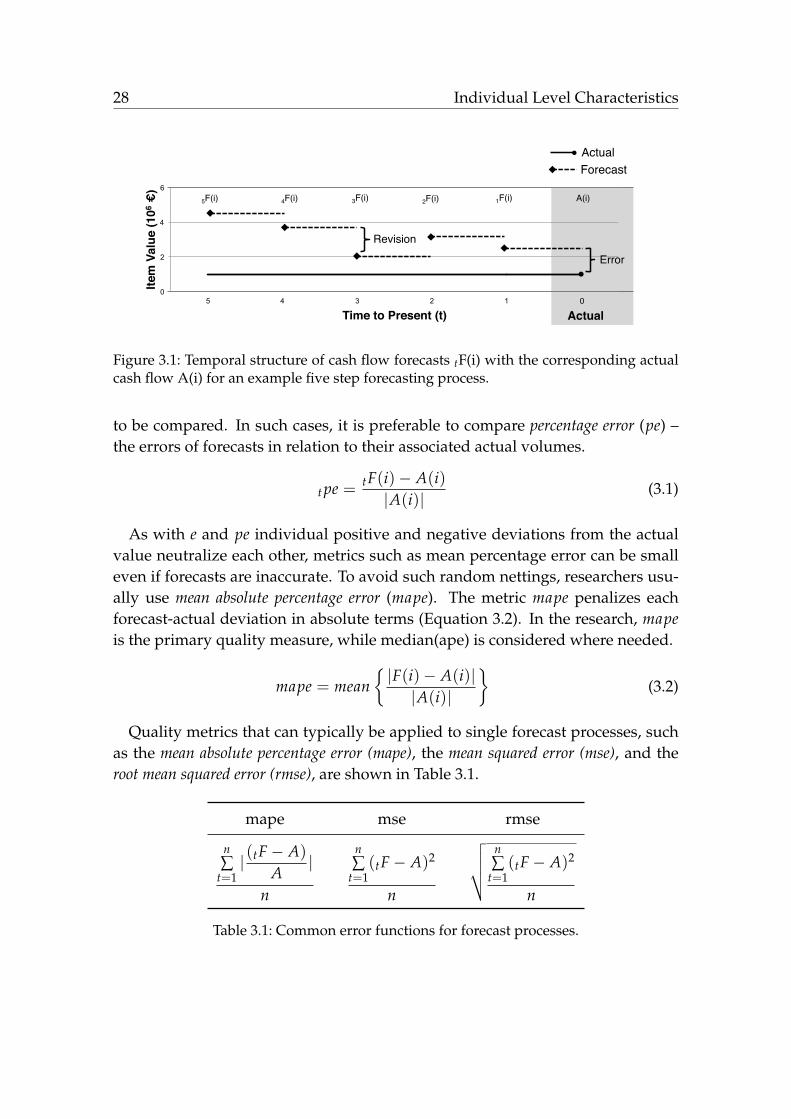
The notation presented in this section is commonly used in current literatureon Nordhaus (1987). Denoting the actual (realization) of cash flow item i as A(i),the lead time t of a forecast tF(i) for A(i) refers to the number of revision periods(i.e., in terms of a quarter of the year) until the actual date (t = 0). For instance,with an initial forecast at t = 5 the earliest forecast 5F(i) is delivered with a leadtime of five periods and is revised four times until the last one–period–aheadforecast 1F(i) is generated. The notation te(i) refers to the forecast error of tF(i),computed as tF(i)− A(i). Figure 3.1 visualizes the temporal structure of a fore-casting process in five steps for an actual A(i).
Subscripts m, y, and s denote the realization month, realization year, and the IDof the corresponding subsidiary of the actual, respectively. Superscript g denotesthe type of the actual (g ∈ {invoice issued (II), invoice received (IR)}) and su-perscript c denotes the standardized three letter currency code (USD, EUR, etc.)1.Therefore, the maximum indexing for an actual is Ag,c
s,y,m(i). If certain informationof an index is irrelevant or obvious in the context, the respective index is omittedfor reasons of brevity. Hence, As=12 refers to the set of all cash flow realizationsof legal entity 12, and 1Fs=12 to the set of all one-period ahead forecasts (lead timet = 1) of this entity.
To assess the accuracy of a group of forecasts (e.g., the long-term forecasts of aparticular subsidiary), usually researchers calculate mean error as the sum of allindividual errors divided by the number of forecasts (Armstrong and Collopy,1992; Shugan and Mitra, 2009). Error-differences in groups, however, are difficultto interpret when item volumes vary substantially within the groups of forecasts
1International Organization for Standardization: Codes for the representation of currencies(https://www.iso.org/standard/64758.html).
27
28 Individual Level Characteristics
0
2
4
6
5 4 3 2 1
Item
Val
ue (1
06 €
)"
Time to Present (t)"
Revision!
Error!
Actual"
5F(i)! 4F(i)! 3F(i)! 1F(i)!2F(i)! A(i)!
Actual!!Forecast!
0!
Figure 3.1: Temporal structure of cash flow forecasts tF(i) with the corresponding actualcash flow A(i) for an example five step forecasting process.
to be compared. In such cases, it is preferable to compare percentage error (pe) –the errors of forecasts in relation to their associated actual volumes.
t pe = tF(i)− A(i)|A(i)| (3.1)
As with e and pe individual positive and negative deviations from the actualvalue neutralize each other, metrics such as mean percentage error can be smalleven if forecasts are inaccurate. To avoid such random nettings, researchers usu-ally use mean absolute percentage error (mape). The metric mape penalizes eachforecast-actual deviation in absolute terms (Equation 3.2). In the research, mapeis the primary quality measure, while median(ape) is considered where needed.
mape = mean{|F(i)− A(i)||A(i)|
}(3.2)
Quality metrics that can typically be applied to single forecast processes, suchas the mean absolute percentage error (mape), the mean squared error (mse), and theroot mean squared error (rmse), are shown in Table 3.1.
mape mse rmse
n∑
t=1| (tF− A)
A|
n
n∑
t=1(tF− A)2
n
√√√√ n∑
t=1(tF− A)2
n
Table 3.1: Common error functions for forecast processes.

Individual Level Characteristics 29
Further, let trV(i) = tF(i)−t+1F(i) denote the directed revision-volume of the t-thlast adjustment of the forecasts for A(i). Hence, the last revision for item i willbe referred to as 1rV(i), the second-to-last revision as 2rV(i), and so forth. Sincethe items vary with respect to their volume levels, the analyses use the relativerevision tr(i), computed as shown in Equation 3.3, which indicates the revision inrelation to the absolute volume of the previous forecast.
tr(i) =tF(i)−(t+1)F(i)|(t+1)F(i)|
(3.3)
Table 3.2 gives a brief overview of the defined notation and metrics.
Notation: Metric:
i Cash flow itemA(i) Actual realizationF(i) Forecastt Lead timem Monthy Years Subsidiary ID, Entity IDg Type of cash flowc Currencye(i) Errorpe(i) Percentage errorrV(i) Revision volumer(i) Revision (relative)mape Mean absolute percentage errormse Mean squared percentage errorrmse Root mean percentage errormedian(ape) Median absolute percentage error
Table 3.2: Notation used for the individual characteristics.
30 Individual Level Characteristics
3.1 Forecast Efficiency
Based on the efficiency theory, Nordhaus (1987) proposed tests for the structureof forecasting processes in terms of correlations amongst revisions and betweenrevisions and errors. Forecast processes that show no correlation structures (withsignificant p-values) are coined weak form efficient.
While t ∈ N+0 denotes the lead time to the realization of an actual (at t = 0),
Nordhaus (1987) suggests testing for weak form efficiency using the Proposi-tions (P1) and (P2).
Proposition 1 (P1). Forecast error at t is independent of all revisions up to (t + 1).
Proposition 2 (P2). Forecast revision at t is independent of all revisions up to (t + 1).
The test in the thesis for weak form efficiency violations uses Spearman cor-relations in a straightforward fashion for the Propositions 1 and 2. The test forProposition 1 determines whether forecast errors te are correlated with revisionjr at any previous position in forecast processes (t ≤ j). Proposition 2 is tested bycomputing correlations within revisions tr with different lead time t. Expectationis that the Propositions 1 and 2 are supported, stating weak forecast efficiency.
3.1.1 Forecast Efficiency: Lead Time
The concept of efficiency is possible to examine in another way, which is morealigned to market efficiency (in reference to Fama, 1970). This thesis suggestsanalysis that will base on the lead time of forecasts and accuracy. When infor-mation is efficiently integrated into forecast processes, the forecasts represent ac-cumulation of all information available. Integration of all information (that arerelevant for the forecasting of an actual) results in forecasts with lower lead timeto contain at least all relevant information of previous forecasts. For instance, thelast forecast should contain all information relevant for forecasting of the actualand therefore exhibit the highest accuracy. If forecasting processes do not inte-grate new, available information into the forecasts or even do miss to integrateinformation that previous forecasts did integrate, a pattern should be identifi-able. The pattern will result in forecasts with lower lead time being associatedwith higher errors, as the beneficial information is missed or even available forintegration. This intention behind this association is proposed within (P3):
Proposition 3 (P3). The decrease of lead time is associated with higher forecast accuracy.
Individual Level Characteristics 31
The thesis’s Proposition (P3) is tested by comparison of accuracy over groupsof forecasts with different lead times. Explicitly, the mape is expected to decreasewithin each set of forecasts with lower lead time t.
3.1.2 Forecast Efficiency Hypothesis: Increased Accuracy
It is argueable that the identification of correlations according to Propositions (P1)and (P2) – maybe at some aggregation levels or after the transformation of theraw forecast and actual items – has potentials to anticipate future adjustments.This is a consequence of existing structures hinting to information that could beincorporated into revisions because revisions are predictable, which might allowaccuracy improvements at longer forecast horizons. The existence of these im-provement potentials for longer forecast horizons require that the forecast pro-cesses do not integrate information according to Proposition (P3).
A violation of these three propositions opens the following three questions:(1) Violation of Proposition (P3) questions if timely efficient integration of infor-mation is beneficial for forecast accuracy? (2) Can information entail forecastprocesses in a way that inefficient forecasting (concerning P1 and P2) is beneficialfor forecast accuracy? (3) Prediction of future adjustments due to inefficienciesrequires that inefficiency must relate to forecast accuracy. Therefore, is efficiencytruly associated to accuracy?
Analysis of these questions should be stated empirically. Since the answersto the first two questions become obsolete by answering the third question withregard to forecast prediction, I intend to analyze the latter one.
Exhibiting the implications of the further analysis clearly requires some the-oretical introduction. The last question breaks down to the general question of“efficiency hypothesis”. Efficiency hypothesis (Fama, 1970) requires forecasts tofollow Equation 3.4, which means that the expected value of an asset j at timet + 1 under information set Φt equals the value p of an asset at time t adding theone-period percentage return r.
Expected Return Theory: E( p̃j,t+1|Φt) =[1 + E(r̃j,t+1|Φt)
]pj,t (3.4)
The efficiency hypothesis, understood as the theory of efficient markets, statesthat if forecasts contain all available information, they will not reveal any tradingopportunities. As a result of Equation 3.4 when all information Φt is integrated,the overall expected return will be zero. Equation 3.5 shows the return and Equa-tion 3.6 shows the expected return. In other words the forecast errors xj,t+1 mustsolely depend on the information Φt being integrated into the forecasts pj,t+1.
32 Individual Level Characteristics
The error may have low or even zero dependency on the integrated informationthat is unimportant. However, integrated important information must reduce theerror and result in a negative dependency of integrated important information tothe error, while inefficiencies should have positive dependency to forecast error.That is because otherwise a forecaster omitting such information would give riseto trading opportunities, which violates the efficiency hypothesis.
Return: xj,t+1 = pj,t+1 − E(pj,t+1|Φt) (3.5)
Expectation of Return: E(x̃j,t+1|Φt) = 0 (3.6)
The efficiency hypothesis received high attention in the research communityand lead to several tests that state different stages of efficiency: strong form, semi-strong form, and weak form. The details of each stage are omitted with referenceto the “expected return theory” based efficiency in Fama (1970). But, importantto note here is that evidence for violation of weak form efficiency will lead to therejection of the strong form efficiency.
Carried out tests for weak form efficiency (such as in Nordhaus, 1987) overa wide range of research papers revealed that the respective empirical analysessuggest both, inefficiency and rejection of inefficiency. With efficiency and ineffi-ciency being stated, the understandable and intriguing substance of the efficiencyhypothesis seems to be widely accepted by the research communities as a fact.
However, despite the persuasiveness of the efficiency hypothesis with a hy-pothesized dependency of efficiency and accuracy (by information being aggre-gated into forecasts) there is a lack of research empiricism2, nor a specific andsuitable testing framework is provided to state the efficiency hypothesis. My sci-entific surprise led to the Hypothesis 1.
Hypothesis 1 (Validity of the Efficiency Hypothesis). In general, efficiency and ac-curacy is not required to relate to each other (in corporate forecast processes).
The hypothesis does not question the existence of efficient and inefficient fore-casting (and markets). Explicitly, this hypothesis questions the validity of theefficiency hypothesis itself, with it’s assumption of efficiency and accuracy beingrelated.
2The research of Lawrence and O’Connor (2000); Dovern and Weisser (2011); Meub and Proeger(2016) (and with limitations: Nordhaus 1987; Bessler and Brandt 1992; Ashiya 2003, 2006) givean indication of the dependence between accuracy and weak efficiency, but are not empiricallyconclusively supported. None of these studies analyzes and tests the dependency directly andeven if one relates the experiments to this question, the sample size ≤ 10 is too small for eachindividual experiment.

Individual Level Characteristics 33
The further intention of this paragraph is to provide a test that is able to statethe Hypothesis 1, and can be applied on empirical data later on. Weak form effi-ciency being a requirement for strong form efficiency, wherefore the constructedtest base on the analysis of the relation of weak form efficiency with accuracy.Following the efficiency hypothesis that violations of Propositions (P1) and (P2)are related to lower accuracy, I explicitly formulate the Proposition (P4).
Proposition 4 (P4). Violations of (P1) and (P2) are associated with lower forecast accu-racy.
The evaluation framework for Proposition (P4) in this thesis bases on absolutecorrelation values, because the interest is in the association of accuracy to thegeneral strength of inefficiency. To avoid random netting effects the mape is takenfor accuracy measure, leading to Equations 3.7 and 3.8 (with a ≥ b) for testing theProposition (P4).
mape(1F(i)) = β0 + β1(|Cor(ar, b pe)|) + ε (3.7)
mape(1F(i)) = β0 + β1(|Cor(ar, br)|) + ε (3.8)
Without current research that questions the validity of Hypothesis 1, the expec-tation for a valid efficiency hypothesis leads to positive β1 estimates. If negativeestimates are found, the efficiency hypothesis must be rejected and Hypothesis 1is supported.
3.2 Anchoring and Adjustment
The question what might cause inefficiencies led to the common anchor of lastyears realizations. To determine whether forecasters use the previous year’s ac-tuals as anchors, the tests are proceeded as proposed in Bromiley (1987). The au-thor suggests that “on average the difference between the anchor and the forecastshould be less than the difference between the anchor and the actual” (Bromiley,1987, p. 202). This results in the two inequations (see Equation 3.9), where theforecast should be typically located between the actual and the anchor κ. Logictransformation results in the equation for ∆ (as computed in Equation 3.10). Neg-ative values of ∆ indicate the presence of an anchor, while positive values rejectthe thesis of anchors.
The intuition is that over a fiscal year the anchoring results can differ for sub-samples based on monthly forecasting groups. For these groups of forecasts at-test is used to determine whether anchors are present.
34 Individual Level Characteristics
κ < F < A or κ > F > A (3.9)
∆ = |κ− F| − |κ− A| (3.10)
Improving the Identification of A&A Patterns
Typically, A&A models focus on the direction of past revisions and assign val-ues with low consideration concerning the strength of the revisions. The Band-width Model (BWM) focuses on the strength of the revisions and assigns a pos-itive value to a positive revision and a negative one to a negative revision. TheBWM assigns a revision to the Up-Group if it is above a certain threshold α andto the Down-Group if it is below −α. Otherwise it is assigned to the Const-Groupas shown in Equation 3.11.
tr ∈ Up⇔t r > α
or tr ∈ Down⇔t r < −α
or tr ∈ Const⇔ |tr| 6 α
(3.11)
This model can be influenced through more parameters than for example Har-vey’s model and is on the other side not vulnerable for small changes in forecasts.The limitation is, that a forecast can only be assigned to three different classes.The results are highly depending on the chosen α, so a second model will be in-troduced. This model is inspired by the BWM, supplemented by an assigningfunction. The assigning functions needs to fulfill the Equations 3.12 – 3.14.
f +(0) = 0 (3.12)
f +(max tr) = 1 (3.13)
f + ′(tr) ≥ 0, ∀ tr ∈ tr+ (3.14)
The function should assign a value of 0 to a revision where no adjustmenthas taken place. The largest revision should further be assigned to 100% to theUp-Group. The function should monotonically increase as the assigned weightshould not lower for higher revisions. As an assigning function that can fulfillthese conditions, the logistic growth function will be used. This function offersa sigmoid process assigning small values for revisions near 0 a value near 1 forlarge revisions and a steady transition near the threshold α. The revisions willbe assigned to a positive and a negative group. The logarithmic growth functionwill be modified so that a weight on every revision can be assigned. The orig-inal logarithmic growth function shown in Equation 3.15 is influenced through

Individual Level Characteristics 35
the saturation limit G, a parameter k influencing the strength of the growth, thefunctions values for revisions of size 0, and the exponential function exp.
fx =G
1 + exp(−kGx)(G
f (0)− 1)
(3.15)
This function is transformed to fulfill the Equations 3.12–3.14. First of all thefunctions value for revisions of 0 should be 0. The function can only convertto 0, for this reason a parameter µ is introduced. The function should convertto this parameter, therefore the parameter should be arbitrary close to 0. Themaximal revision should be valued as 1, the saturation limit G is therefore setto 1. Additionally the turning point should be 0.5. In a next step the function isshifted with the value of α so that the values in Equation 3.16 are reached.
f(0) = 0.5 and f(−α) = µ (3.16)
The parameter k can be predicted in dependency of µ and α, as shown in Equa-tion 3.17, where ln is the logarithmic function.
k =
ln(1µ− 1)
α(3.17)
Re-shifting this function with −α is resulting in Equation 3.18 and Equa-tion 3.19 that differentiate between positive and negative revisions. These equa-tions are showing the functions for the Logistic Bandwidth Model (LBWM), wherenegative revisions are handled in the same way as positive revisions, except forchanging the sign of the revision.
f +log(tr) =
1
1 + exp
ln (1µ− 1)
α
(−tr + α)
(3.18)
f −log(tr) =1
1 + exp
ln (1µ− 1)
α
(tr + α)
(3.19)

36 Individual Level Characteristics
Figure 3.2: Logistic assigning function for anchoring probability of forecasts with positiveand negative revisions.
Finally this results in two different new models for detection of A&A effects.The Bandwidth Model classifies all forecast in three different groups, assigningthree different values on them. The Logistic Bandwidth Model classifies the fore-casts in two different groups complemented by a weight for A&A effects. Basedon the two provided models the Propositions 5 and 6 will be evaluated.
Proposition 5. Bandwidth Models can provide beneficial information to identify anchor-ing and adjustment effects that relate to forecast accuracy.
Proposition 6. The relation of the Bandwidth Models to other anchoring and adjustmentmodels depend on the forecast series.
The evaluation uses five synthetic forecast series and three loss functions forthe comparison of the two Bandwidth Models BWM and LBWM with commonA&A models (Bromiley, 1987; Harvey et al., 1994; Lawrence and O’Connor, 1992;Amir and Ganzach, 1998). Each of the mentioned models detects A&A effectsin a different way, which will be adjusted to the synthetic series as in (Knöll andRoßbach, 2018b). In real world forecast series it is difficult to relate forecast seriesto one unique A&A pattern and to identify dependencies between the patternand the models. Therefore, synthetic forecast series were generated with specifickind of A&A pattern influencing the forecast series. The synthetic series allow acomparison of the identification performance of the different models, as a controlfor the underlying pattern is feasible. The different forecast series are expected torelate to (or even occur in) real world forecasts.
Three of the five series base on a normal distribution with no or only low trend:independent (Ind), random walk without trend (RW-1), and random walk with trend
Individual Level Characteristics 37
(RW-T). Two series are used to simulate a stronger growth component: logarith-mic growth (LogG), and exponential growth (ExpG). Each type of forecast series con-sists of 1000 observations. The independent series consists of normal distributedseries with an expected value (µ) of 1000 and a standard deviation (σ) of 1. Therandom walk series are based on normal distributed steps, x0 = 1000, a µ of 0,and a σ of 1. The random walk series with trend are defined through normaldistributed steps, a starting value of x0 = −1000, a µ of 2, and a σ of 1. The log-arithmic growth series consists of logarithmic growing forecasts, with a uniformdistribution of the basis between 0.1 % and 3.0 % starting by x0 of 100. Last of all,the exponential growth series will consist of forecasts with exponential growthwith growth rates uniform distributed between −100 % and 100 % starting by x0
of 1000. For example, the random walk series were generated with Equation 3.20.
xn = x0 +6
∑t=1N (µ, σ2) (3.20)
For each synthetic forecast process in each forecast series, all the different mod-els calculate the probability value ν of an anchor and adjustment pattern. Theprobability in each forecast process is determined by the absolute mean proba-bility of anchoring |mean(ν)| of all revisions within the process. Explicitly, theforecast processes have a maximum lead time t = 5 (based on real forecastprocesses), which results in four probability values: ν f (tr) with t ∈ {1, 2, 3, 4}.The model BWM indicates ν f=BWM(tr) with percentage values of 100 %, 0 %, or−100 % (according to the classes: Up, Const, Down), whereby positive and nega-tive values cancel each other out. The LBWM provides continuous probabilitiesfor ν f=LBWM(tr) with percentage values in the interval [100 %, . . . ,−100 %]. I.e.,the BWM assigns an anchor probability of 50 % to a forecast process with threerevisions of the Up-Group and one revision of the Down-Group.
Finally, for each set of forecast series the probability of the models are Pearsoncorrelated with the mse, rmse, and mape error measures (see Table 3.1) to analyzeProposition 5. Further, the evaluation will analyze the correlations between themodels in order to support Proposition 6.
3.3 Optimism, Pessimism and Overreaction,Underreaction
In order to determine whether the bias-related patterns “optimism, pessimism”and “overreaction, underreaction” are present in the forecasts, the test design is

38 Individual Level Characteristics
followed as proposed by Amir and Ganzach (1998). From their analysis of fore-casts, the authors conclude that overreaction and underreaction operate concur-rently with optimism and pessimism.
Optimism refers to cases where the last forecast exceeds the actual (1F > A).Pessimism refers to cases where the last forecast lies below the actual (1F < A).Overreaction describes the case of revisions being greater than required (e.g., fort = 1: 1r > 0 > 1pe; revision and error have different directions). Underreactiondescribes the case of revisions being too small (e.g., for t = 1: 1r and 1pe have thesame sign).
The results reported by Amir and Ganzach (1998) indicate that the strengthof these patterns decreases with lead time. This finding makes sense intuitively,since more reliable information becomes available as one approaches the actualdate, leaving less room for speculation and strongly diverging expectations.
Following the methodology of Amir and Ganzach (1998, pp. 339–341), thetest measures the strength of optimism, pessimism, overreaction or underreac-tion with the parameters learned in the regression shown in Equation 3.21. Incontrast to Amir and Ganzach the tests use standardized revisions on the basis offorecasts with subsequent lead times and standardized errors on the basis of actu-als. Positive α’s indicate optimism, negative α’s pessimism. Positive β’s indicateoverreaction, negative β’s underreaction.
t pe = α(t) + β(t)tr + ε (3.21)
3.4 Revision Concentration
Anchors that influence forecasts could not only have an influence on the error,but could also show divergent effects for the error at different points in time. Thisargument refers to the work of Knöll et al. (2016). The work studies whether spe-cific structures (in contrast to random walks) in forecast processes are observable,whether these are related to accuracy, and how knowledge on such patterns canbe used to statistically correct the forecast in order to reduce error in the exposureprediction.
Geometric Center
To test whether structures (in contrast to randomness) in revisions relate to con-centration, this paragraph proposes to determine the geometric center of a revi-sion process. The geometric center of a revision process is computed as follows.First, each revision is set into relation to the first forecast, and normalized by

Individual Level Characteristics 39
the sum of all revisions relative to the first forecast, as shown in Equations 3.22and 3.23. The coordinates for the geometric center are computed with Equa-tions 3.24 – 3.26.
1t r(i) = tF(i)− t+1F(i)
|1F(i)| (3.22)
xt r(i) =
1t r(i)
Σt|1t r(i)|(3.23)
xi = −2 · |xt+3r(i)| − 1 · |xt+2r(i)|+ 1 · |xt+1r(i)|+ 2 · |xt+2r(i)| (3.24)
yi =Σt
xt r(i)2 − 0.25(1.0− 0.25)
(3.25)
zi =Σt
xt r(i)4
(3.26)
If revisions follow a random walk without drift, a mean center (x0,y0,z0) in asubsample of processes will be observed. A value of x < x0 indicates that largeradjustments are made earlier in a revision process (timing). Larger y (comparedto y0) indicate a higher concentration of adjustments at a specific revision in aforecast process (volume). Positive z indicate that, overall, revisions are positive,i.e. the extent of upward revisions during the process is greater than of down-ward revisions (direction).
Take, for instance, a revision process with 1r(i) = 1 and 2r(i) = 0 and 3r(i) = 0and 4r(i) = 0, i.e., the forecast is revised only once at the end of the revision pro-cess. The coordinates for this process are then (xi,yi,zi) = (2,1,0.25), indicating thatrevisions were concentrated at the end of the revision process, more specifically:in one revision, and that this revision was positive. With p(i) as the forecast re-vision process for item i and P as a set of forecast revision processes for differentitems i, the following Proposition 7 is formulated.
Proposition 7. The average geometric center of a set of forecast revision processes Pmust not deviate significantly from (x0,y0,z0).
The test of Proposition 7 uses Wilcoxon rank sum tests on mean differences offorecast processes for x,y and z measures.
Change in Error Level
Now the question is turned on whether the concentration measures provide ex-planation value for the error term, which is required to correct forecasts by using

40 Individual Level Characteristics
concentration measures. The analyses will measure the change between the er-ror level of the first and last forecasts (5F and 1F) in terms of ape, described inEquation 3.27.
change in error level : ∆5,1 = |5pe| − |1pe| (3.27)
Considerable error rates are particularly important in this analysis of the data,which is why the data is reduced to forecasting processes where the ape of 5F isgreater than 5 %. The analysis of ∆5,1 will base on the explanation value of theconcentration measure in comparison to metrics required for inefficiency. For thispurpose the linear regression model bases on Equation 3.28 and 3.29. The test willcompare explanation values with the R2-value of both regression models. It isimportant to note that the regression will be evaluated for different set of forecastprocesses split by the sign of error pe (positive, negative), wherefore the resultsare independent from absolute forecast numbers (such as 1F).
∆5,1 = β0 + β1(4rV) + β2(3rV) + β3(2rV) + β4(1rV) + β5(g)+
β6(Division) + β7(Sign change (none)) + β8(Sign (positive)) + ε(3.28)
∆5,1 = β0 + β1(xi)× β2(yi)× β3(zi)× β4(g) + ε (3.29)
The final descriptive analyses will examine the Y metric (volume concentra-tion), which is interesting in particular with regard to the empirically unsup-ported statement in Leitner and Leopold-Wildburger (2011, p. 466) that “largeadjustments of forecasts improve accuracy most, and small adjustments harmit”. This statement is questioned in Hypothesis 2.
Hypothesis 2. Revision processes might be harmed by small forecast adjustments, re-ducing forecast accuracy.
The distribution of revision volume is expected to indicate at which time theintegration hint to important information, most likely to exceed random noise3.Therefore the analysis of the Y concentration measures will provide detailed in-formation for different types of revision processes and how the metrics interactwith each other. The analyses will base on how the Y metric interact with X
3For example, adjustments of 1 Euro are considered unimportant (to the forecast process) whenthe forecast volume is 1 million Euro and typical revisions amount to ten percent of this fig-ure. Such unimportant adjustments could be framed as random noise in forecast processesgenerated by forecasters to indicate their active involvement.

Individual Level Characteristics 41
(timing concentration) and Z (direction concentration) with regard to the errorlevel ∆5,1. The first part will analyze ∆5,1 of the data based on Y and Z measuresin dependency to item type (g) and over-/underestimation. The second part willanalyze ∆5,1 of the data in dependency to Y and X measure.

Chapter 4
Aggregate Level BusinessCharacteristics
This thesis argues that some useful structures in revisioning might only befound at particular transformation and aggregation levels of the data, re-
quiring the engineering of features from the data. The engineering of features,i.e., their aggregation, selection, and representation, requires a solid understand-ing and modeling of business and organizational structures.
4.1 Ratio Metric
Because the planning for the fulfillment of the corporation’s targets is determinedon an aggregate level the cash flow forecasts are accumulated up to this level.For the return–related analyses at the organizational level, the abstraction has theform of an aggregated perspective of cash inflows and cash outflows for actuals(and for forecasts).
4.1.1 Construction Process
As a proxy for percentage return margin within a fiscal year for a specific sub-sidiary, the computation of the entity’s ratio R uses aggregated revenues (invoiceissued) and expenses (invoice received).
Definition 1 (Ratio). The ratio for an specific subsidiary (s = S) in the M-th month ofa year Y and the K months (K < M) before M is computed as:
RKs=S,y=Y,m=M(A) =
∑1≤j≤K Ag=I Is=S,y=Y,m=M−j
∑1≤j≤K Ag=IRs=S,y=Y,m=M−j
while:
43
44 Aggregate Level Business Characteristics
Y = specific year
M = specific month
K = aggregated number of months
S = specific subsidiary
As with individual actuals and forecasts, the use of lead time t > 0 refers to ratios com-puted over forecasts (tF) noted as tR; the ratios over individual actuals (A) noted as 0R.
For instance, tR32010,11 refers to the ratio with lead time t of all cash flows from
September to November 2010. The notation tRKY,M omits the superscript K, if K =
M− 1, and is an aggregation of all realized cash flows in year y = Y up to (andincluding) month m = M. The usage of the indices (s, c) specifies particular datasets for 〈subsidiary, currency〉-tuples. A ratio above one indicates the appearanceof more revenues than expenses (positive return).
Since ratios are specific for each subsidiary s, for reasons of comparability, thisthesis focuses on normalized ratios Rn (Definition 2). For the readers conve-nience, if not specifically relevant for differentiation, the notation tR refers to thenormalized ratio instead of the entity specific ratio (tRs=S := tRn
s=S).
Definition 2 (Normalized Ratio). Normalized ratio is obtained by subtracting the min-imum ratio within an entity from R and dividing by the difference of its maximum andminimum ratio. The values are always between zero and one per entity.
tRns=S,y=Y,m=M =
tRs=S,y=Y,m=M −min(⋃
R)max(
⋃R)−min(
⋃R)
while: ⋃R = {tRs,date : s = S ∧ date < (Y, M)}
The proxy for the suggested annual return target (target ratio) for an entity s = Sis defined as T(0R)y in year y. As subsidiaries’ targets are unknown (to me), butbusiness development measured with EBITDA margin figures seems to be ratherstable over the years, the target is calculated on the basis of Definition 3.
Definition 3 (Target). The target ratio in year y = Y is estimated by averaging theDecember actual ratios of the three preceding years. It is formally defined as:
T(0R)y=Y = mean(0Ry=Y−j,m=12), with j ∈ {1, 2, 3}
Alternatively, one could use the EBITDA margin figures provided in the officialannual reports to retain a proxy for target margins. But, since this thesis analyzes

Aggregate Level Business Characteristics 45
predictive purposes too, and numbers of the annual report are expected to con-tain several business adjustments, the aforementioned data-driven approach ischosen.
Definition 4 (Target Difference). The difference from target is defined as:
TargetDiff = T(0R)− 1R
Definition 5 (Revision). The revision of ratios describes the adjustment from the secondto last forecast before the actual. It is formally defined as:
12R = 1R− 2R
This thesis uses the last revision because generally the latest judgmental fore-cast incorporates the most information and is the most accurate (McNees, 1990).
Definition 6 (Ratio Error). Finally, the error of forecast ratios is defined by:
1E = 0R− 1R
For reasons of clarity: Ratios and revisions are not stored in the database, butderived from the aggregation of invoice items as shown in Definition (1). Table 4.1gives a brief overview of the defined metrics.
Notation: Metric:
0R Actual Ratio (normalized) Definition 1 for A(i)tR Forecast Ratio (normalized) Definition 1 for tF(i)T(0R) Target (normalized) Definition 3TargetDiff Target Difference Definition 412R Revision Definition 5tE Error Definition 6
Table 4.1: Notation used for the aggregate characteristics.
Denoting the actual of cash flow margin ratio as 0R, the lead time t > 0 of aforecast tR for 0R refers to discrete process steps until the actual date (t = 0).Figure 4.1 visualizes the temporal structure of an example forecasting process infive steps for an actual 0R. The initial forecast ratio 5R is delivered with a leadtime of five periods and is revised four times until the last one–period–aheadforecast ratio 1R is generated.
Analyses at the ratio level are important as they are supposed to be directlyrelated to foreign exchange exposure, which strictly relates to the accumulated
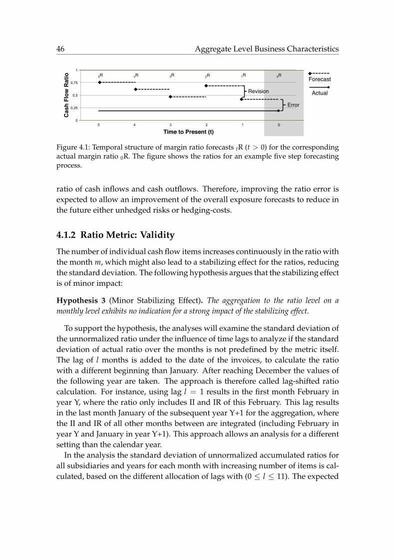
46 Aggregate Level Business Characteristics
0
0,25
0,5
0,75
1
5 4 3 2 1
Cas
h Fl
ow R
atio!
Time to Present (t)!
Revision!
Error!
5R! 4R! 3R! 1R!2R! 0R!
Actual!
Forecast!
0!
Figure 4.1: Temporal structure of margin ratio forecasts tR (t > 0) for the correspondingactual margin ratio 0R. The figure shows the ratios for an example five step forecastingprocess.
ratio of cash inflows and cash outflows. Therefore, improving the ratio error isexpected to allow an improvement of the overall exposure forecasts to reduce inthe future either unhedged risks or hedging-costs.
4.1.2 Ratio Metric: Validity
The number of individual cash flow items increases continuously in the ratio withthe month m, which might also lead to a stabilizing effect for the ratios, reducingthe standard deviation. The following hypothesis argues that the stabilizing effectis of minor impact:
Hypothesis 3 (Minor Stabilizing Effect). The aggregation to the ratio level on amonthly level exhibits no indication for a strong impact of the stabilizing effect.
To support the hypothesis, the analyses will examine the standard deviation ofthe unnormalized ratio under the influence of time lags to analyze if the standarddeviation of actual ratio over the months is not predefined by the metric itself.The lag of l months is added to the date of the invoices, to calculate the ratiowith a different beginning than January. After reaching December the values ofthe following year are taken. The approach is therefore called lag-shifted ratiocalculation. For instance, using lag l = 1 results in the first month February inyear Y, where the ratio only includes II and IR of this February. This lag resultsin the last month January of the subsequent year Y+1 for the aggregation, wherethe II and IR of all other months between are integrated (including February inyear Y and January in year Y+1). This approach allows an analysis for a differentsetting than the calendar year.
In the analysis the standard deviation of unnormalized accumulated ratios forall subsidiaries and years for each month with increasing number of items is cal-culated, based on the different allocation of lags with (0 ≤ l ≤ 11). The expected
Aggregate Level Business Characteristics 47
result, if the stabilizing effect exists, is that standard deviation does reduce contin-uously from the month on that the aggregation started (framed as “1st Month”) tothe last month (framed as “12th Month”). If the standard deviation does not de-crease in general until the last month, the analysis will refuse a strong stabilizingeffect and support Hypothesis 3 to state the validity of the ratio construction.
4.1.3 Ratio Metric: Earnings Target Existence
EBITDA Figures
Before describing the design for this section of the empirical study, this sectionwill briefly review the intuition of the design.
EBITDA figures are a primary KPI for corporate performance, and many cor-porations incentivize their managers to meet such prearranged KPI targets. Theoverall intuition is that meeting prearranged EBITDA targets is well incentivizedand should therefore predefine the way on how aggregated actuals will developover a year, and, as a consequence, how cash flow forecasts will (have to be)adjusted. The feature that this thesis considers is the subsidiary’s ratio of cash in-flows and cash outflows accumulated over a fiscal year – a figure tightly relatedto a KPI such as EBITDA.
For the hypotheses, it is therefore assumed that the derived target ratios arelinked to the percentage EBITDA margin figures of the company. This assump-tion seems to be plausible for two reasons. (1) Realized revenues (through in-voices issued) and expenses (through invoices received) will later result to thederived EBITDA margins. (2) This assumption would be underpinned by the re-ported percentage EBITDA margin figures published in the annual report, if theyare in line with the ranks of division ratios for December values.
The fulfillment of the second reason allows to advocate the retainment of asubstitute for percentage EBITDA margins with ratios on a monthly basis.
Decrease of Standard Deviation
The assumption of the margin targets should be underpinned statistically. If mar-gin targets are present, the 12th month should have decreased standard deviationcompared to the 1st month. An indication that targets possibly exists and mightbe met early, would be provided if the standard deviation reaches its minimumbefore the 12th month.
The constructed test will analyze the standard deviation of normalized ratios,for specific lags where Hypothesis 3 is supported, i.e. in the fiscal year, to considernumerical differences between subsidiaries.
48 Aggregate Level Business Characteristics
Ratio End of Year Drifts
Further support for the existence of the target will be provided by a median ratioanalysis over time for the subsidiaries, which will be grouped into the associateddivisions. The analysis will study whether the ratio feature will drift towardsthe end-of-year ratios of the preceding years. The examination focuses whetherthere are regular and strong shifts of aggregated cash-in/cash-out volumes inthe ratios towards the end and beginning of the fiscal year. In the absence ofearnings management, ratios could stabilize over the course of a fiscal year asactuals accumulate, but there should be no discernible pattern in the changes ofratios between December and January.
4.1.4 Ratio Metric: Subsidiary Specific Revision
First analysis for the revision questions if the normalization helps to identify spe-cific pattern of the subsidiaries’ adjustments in ratio. The test will analyze therevision of all subsidiaries being made with regard to the error, based on un-normalized and normalized ratio figures. Indication of the importance of thenormalization will be provided by visualization of 12R and 1E.
4.2 Efficiency at Aggregate Level
Weak forecast efficiency can be tested by using Propositions 1 and 2. The inten-tion is that efficiency can differ for different aggregation levels, and biases thatmight matter at the individual level might be of no concern at an aggregate level.For instance, an organizational bias on the aggregate level might distort individ-ual forecast, but with regard to the aggregate level the influence of individualbiases might vanish. Therefore, the following paragraphs proposes a theoreti-cal framework to unite findings of both levels – individual and aggregate level –before analyzing the efficiency at the aggregate level further.
4.2.1 Reasoning Beneficial Inefficiency in Individual Forecasts
Thesis suggests that organizational biases need to be analyzed together with orbefore individual biases. Otherwise, the results from analyzing individual biasesmay be confounded, which ought to result in violations of Proposition (P4). Forinstance, organizational biases such as earnings targets can trigger earnings man-agement activities, which results in shifts of cash flows into the next month or tothe previous ones – depending on item type of expense or income. Upcoming
Aggregate Level Business Characteristics 49
actual values that are shifted in a subsidiary might differ structurally from theactual item values of the subsidiaries with no shifts. These actual shifts result inerrors that a uninformed forecaster can not account for at all. The resulting indi-vidual level errors and seemingly individual level biases might be questioned forsuch a confounding influence. In other words, if inefficient forecasts are associ-ated with higher forecast accuracy, organizational biases may be at play, which isformulated in Proposition (P8).
Proposition 8 (P8). Organizational bias generates violation of (P4).
Support of the Proposition 8 should be provided with an explanation frame-work that associates the organizational biases with the violation of Proposi-tion (P4). This means that the information available on a case-by-case basis,which is determined among other things, from the examined biases, should bebrought in line with the efficiency perspective. Using the results from the testof the validity of the efficiency hypothesis (Equations 3.7 and 3.8), this work oncorporate forecasts focuses to offer a consolidating perspective. The confoundinginfluence is considered to be found if the explanation of the differences betweenviolations and non-violations can conclusively base upon the association of theorganizational biases.
4.2.2 Testing Aggregate Level Efficiency
On the aggregate level the efficiency of the corporate data will be tested, usingPropositions 1 and 2. The efficiency test analyzes Spearman correlation of revi-sions t,t+1R with previous revisions j,j+1R (j < t), and correlation of revisionst,t+1R with errors jE (j ≤ t). Expectation is that on the aggregate level efficiencyis not given, indicating the existence of organizational biases.
4.3 Organizational Relations
Experts might be not fully aware of targets and earnings management activities.A further challenge is that there are no direct observations of earnings manage-ment or other potentially bias-related activities. With such information available,it would become much easier to disentangle the effects of different biases on fore-casting processes.
When earnings management takes place and the exact figures for cash trans-fers are unavailable, which is usually the case, the organizational target mightreveal pattern in which way incentives alter forecasts and accuracy. Such found

50 Aggregate Level Business Characteristics
pattern can lead to automated correction of longer–term forecasts by anticipationupcoming revisions and errors. Research results from other domains (such as inearnings forecasts) are transferred to proxies of return margins to apply findingsto the domain of cash flow forecasting.
This paragraph provides the following contributions to the literature: First,analyses cover the dependency between target and error to identify if knowledgefor the target extends traditional knowledge and to uncover possible correctionopportunities. Second, it is argued that pursuing annual return targets introducesan organizational bias, the pattern of concealed information (introduced later),which systematically influences the forecast revisions. The section analyzes theratio to provide evidence that forecast and their revisions provided probably donot reflect the entire internal view of a subsidiary. Third, analyses quantify de-pendencies of the assumed organizational bias on the purpose of forecasting pro-cesses. Here, the intention of the analyses is to reveal that managed cash flowearnings and pursued targets distort forecast revisions, thus undermining thecorporate original goal of the forecasting process – to receive an accurate repre-sentation of upcoming cash flows. The subsequent sections explain and presentthe test design for the hypotheses.
4.3.1 Error Dependencies on Earnings Target
In order to investigate further the case of organizational biases induced byplanned targets and earnings management, this section conducts the analyses onthe organizational level. In particular, this section designs the analyses whetherregular patterns in the subsidiaries’ revision process made by the managers’ cashflow forecasts can be exploited to improve the forecast accuracy by consideringproxies of key figures.
As noted before, reaching margin targets is an important organizational goal.The expectation with regard to the importance is that a statistical model has ahigher explanatory power when additional key figures of planning and oper-ations are provided, namely the Target listed in Table 4.1, which motivates thefollowing hypothesis:
Hypothesis 4 (Incorporation Beneficial for Explanatory Power). Incorporation ofkey figures (that organizationally biases forecasts) has a beneficial influence on the ex-planatory power of forecast correction models.
The influence of the integration of such a key figures can be measured in threeways: by the R2-value of the model (explanatory power), by a meaningful esti-

Aggregate Level Business Characteristics 51
mate for the variable of the key figure, and finally by out-of-sample tests (coveredin Chapter 5).
The support for the Hypothesis 4 will be provided by the following analysisconducted on the empirical study. Two linear models are regressed on the ratioerrors 1E (difference between the actual ratio and the forecast ratio, computedover the final forecasts) using given data. The first linear model only uses statisti-cal information: a constant for regression intercept, last forecast ratio 1R, and lastrevision 12R. In order to examine whether high ratio errors are associated withhigh differences between forecast and target ratio, the second linear regressionmodel uses a regression intercept, last forecast 1R, last revision 12R, and addi-tionally the information of business key figures, difference from target DiffTarg.The two regression models are shown the Definitions (7) and (8).
Definition 7 (Basic statistic model MBasic).
1E = β0 + β1(1R) + β2(12R) + ε
Definition 8 (Organizational model MOrga).
1E = β0 + β1(1R) + β2(12R) + β3(TargetDiff ) + ε
Explanatory Power in Analytic Correction Models
The influence on the explanatory power of additional information can be shown,by using R2-values that describes the part of variance being explained by themodel. The effect of increasing the R2-value is an important indicator for thebeneficial information added, measured by the additional amount of variance ex-plained. For the linear regression models the R2-values will be compared withinan in-sample training period. The R2-value of the model using the business keyfigures (TargetDiff) must be greater than the model without that information inorder to support Hypothesis 4.
Significant Influence of the Estimate
The second analysis examines whether ratio errors 1E increase with the differencebetween the forecast and the assumed target ratio (TargetDiff ). The expectation isan estimate of TargetDiff > 0, in particular towards the end of a fiscal year. Thesignificance of the estimate will provide support that the business key figure hasa non-random influence.
If forecasters have at least partial foreknowledge whether targets have beenmet and earnings will be managed, they can integrate this knowledge into their

52 Aggregate Level Business Characteristics
earlier forecasts. As a result, one would expect to observe only a weak relation-ship between forecasts 2R and 1R, and last revision 12R would seem independentfrom ratio error (insignificant estimate of ≈ 0) at the end of the year.
The test will analyze the regression estimates for the full year in comparisonto the regression estimates for a models based on December actuals. Further, thetest will analyze the December model to a model based on January actuals.
4.3.2 Dependencies on Revision
This section designs the analyses to determine whether regular patterns in thesubsidiaries’ aggregate level revisioning process, which result from the cash flowforecasts of the forecasters, can be exploited by anticipating subsequent adjust-ments.
Revision: Direction and Strength Influenced by Targets
Suggesting an accountant within a legal subsidiary to aim at achieving a prede-fined EBITDA margin, the magnitude of changes in ratio as a result of cash flowrevisioning should increase with the distance to a presumed target. As it is as-sumed that the target ratio has to be met at the end-of-year, the difference fromtarget should decline over the months of the year. Therefore, the predefined cor-porate planning figures of EBITDA margins motivate the following hypothesis:
Hypothesis 5 (Predefined Revisioning). Corporate planning can pave the way forrevision adjustments in decentralized forecasting processes (as an organizational bias).
Explicitly, expectation is a dependency of the target ratio (T(0R)) and revision(12R), together with a decrease of adjustments over time when the current forecastratio approaches the suggested target. A schematic illustration of the expectedrelationships is shown in Figure 4.2. In order to support Hypothesis 5 this thesisconducts several analyses to test this relationship:
(1) The regression analyzes the magnitude of 12R on strength of TargetDiff to-gether with the actual month within a fiscal year (Month), using Definition 9.
(2) In order to operationalize these dependencies to improve cash flow predic-tion, information is required for the direction of the final change in the forecastratio. Therefore, revision 12R is regressed on the strength of TargetDiff and Month,using Definition 10.
(3) However, the interpretation of the regression outcomes when a forecast ra-tio is already above the suggested target is challenging. Therefore, analysis covershow forecast ratios are revised when suggested targets are already reached with
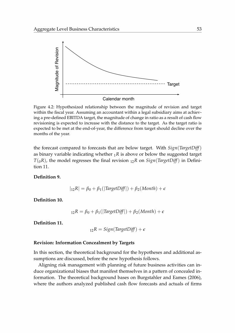
Aggregate Level Business Characteristics 53
Calendar month!
Mag
nitu
de o
f Rev
isio
n!
Target!
Figure 4.2: Hypothesized relationship between the magnitude of revision and targetwithin the fiscal year. Assuming an accountant within a legal subsidiary aims at achiev-ing a pre-defined EBITDA target, the magnitude of change in ratio as a result of cash flowrevisioning is expected to increase with the distance to the target. As the target ratio isexpected to be met at the end-of-year, the difference from target should decline over themonths of the year.
the forecast compared to forecasts that are below target. With Sign(TargetDiff )as binary variable indicating whether 1R is above or below the suggested targetT(0R), the model regresses the final revision 12R on Sign(TargetDiff ) in Defini-tion 11.
Definition 9.
|12R| = β0 + β1(|TargetDiff |) + β2(Month) + ε
Definition 10.
12R = β0 + β1(|TargetDiff |) + β2(Month) + ε
Definition 11.12R = Sign(TargetDiff ) + ε
Revision: Information Concealment by Targets
In this section, the theoretical background for the hypotheses and additional as-sumptions are discussed, before the new hypothesis follows.
Aligning risk management with planning of future business activities can in-duce organizational biases that manifest themselves in a pattern of concealed in-formation. The theoretical background bases on Burgstahler and Eames (2006),where the authors analyzed published cash flow forecasts and actuals of firms
54 Aggregate Level Business Characteristics
as a function the expectations of market analysts. While Burgstahler and Eamesfocus the management of cash flows on the outer shell of firms, the proposedanalysis cover the internal forecasts and actuals within the sample corporation.In contrast to Burgstahler and Eames (2006), the following hypothesis should beconsidered as an extension by referring the shifts of earnings management to aspecific reason based on empirical data. Further, the data will cover the internalforecasts and actuals of the corporation, from which official market reports arederived later on.
The difficulty for corporations lies in their need for a well–aligned manage-ment of planning, forecasting, and operations. To align the management to re-cent, current, and future business development, the corporation requires infor-mation from the subsidiaries. Information is usually provided through managers(and information systems) that have the possibility to access a perspective on theinternal state of the subsidiary, which often requires preprocessing informationto a view required by the corporation. The amount of work involved in planning,forecasting, and operations often implies sharing of tasks by several managers.When organizational structure motivates one manager (e.g. with incentivizationpayment), but not the other ones, an organizational biased view might occur forsome of the information–giving managers. As a result, organizational biased fore-casters might provide a view that incorporates inaccuracies in the forecast data.These inaccuracies originate partly from the concealment of information—whenmanagers with the different tasks are not well aligned and one side is hiding in-formation (unintentionally). Hence, the following hypothesis is made:
Hypothesis 6 (Information Concealment). Organizational biases can result in fore-casting that follows a pattern defined as the “concealment of information”.
As noted before, reaching planned targets is an important organizational goal.If forecasts are adjusted to follow these targets, a pattern of concealing informa-tion inside the subsidiary may occur. The resulting pattern for Hypothesis 6 willdrive adjustments differently for revisions regarding their current position. Thepattern is an indication of the prevention of bad news. Here, the performanceabove the target is perceived as good current state. In order to conceal bad news,adjustments should increase more strongly when the performance is bad (or notas good as required) and should decrease with a good performance – but not asfast as bad news. As a result, some of the good news can be held back for worsetimes of the subsidiary.
The expectation on Hypothesis 6 with regard to end of year targets (in align-ment to Hypothesis 5) leads to a decrease of adjustments over time, as the current

Aggregate Level Business Characteristics 55
forecast ratio approaches to the target. A schematic diagram of the expected ad-justments is given in Figure 4.3.
Calendar Month!
Rev
isio
n to
war
ds T
arge
t!
Target!
Figure 4.3: Required pattern that adjustments follow to conceal bad news. Current per-formance below the target increases the revision upward and performance above the tar-get decreases the revision. The magnitude of revisions for performance below the targetshould be much higher compared to a performance above the target.
To test the relationship, the regression for 12R uses one boolean variables for therelation between target and forecast ratio (TargetDiff(+)), while the other state ofthe boolean variable is indicated by the intercept. Therefore, the intercept is re-named to “TargetDiff(−)”. Further the regression uses the month and interactioneffects of month and TargetDiff(+). The linear regression is modeled with theDefinition 12.
Definition 12 (Information Concealment).
12R = β0(TargetDiff(+)) + β1(TargetDiff(−)) + β2(Month)+
β3(TargetDiff(+) ×Month) + ε
while: TargetDiff(+) = true (equals one) indicates a forecast below the target,
TargetDiff(−) = true (equals one) indicates a forecast above the target,
Month = the number of the month in the fiscal year, and
TargetDiff(+) ×Month = interaction of the target relation and the month of the
fiscal year, stating that the forecast is below the target.
4.3.3 Impact on Organizational Goals
The subsequent analyses in this paragraph are proposed to alter the corpora-tion’s understanding of the meaning of “the goal of forecasting” in forecasting
56 Aggregate Level Business Characteristics
processes. After the analysis of organizational biases in subsidiaries (target in-fluence, revisions predefined, and concealment of information), it will be ana-lyzed whether corporate operations are well aligned to the goal of accurate fore-casting. Structures in organizational operations might alter the realizations (e.g.,with earnings management) that are compared to the forecasting figures. Thesechanges can have serious implications on forecast error measures. Therefore,Proposition 8 and Hypothesis 6 motivate the Hypotheses 7 and 8. These new hy-potheses aim at disentangling the “goal of forecasting” for corporations from themanagerial “goal of forecasting”, as organizational influences are to be expectedto alter the former goal.
The intention behind the corporation’s “goal of forecasting” is that forecastersshould provide perspectives for future expectations and should try to minimizethe forecast error, which can be understood as an organizational bias itself onforecast processes. The assumption is that forecasting process might have a ran-dom baseline, but more importantly, to underline the foretold intention, in a fore-cast process the forecasting adjustments should depend on actual realizations.This leads to the following Hypothesis 7.
Hypothesis 7 (Distorted Forecast Processes). Structures in organizations (as a bias)can alter or distort forecasting processes.
When the tasks of planning, forecasting, and accounting are interlinked tosome extent, the pursuit of planned annual return targets can systematically in-fluence both actual and forecast adjustments, which requires a comprehensiveperspective. Tasks of forecasting, planning, accounting operations can be as-signed to different managers. Forecasters who actually focus to intentionally givepurposeful forecasts can, however, provide organizationally biased forecasts – inrelation to Hypothesis 6 – suggesting a trade-off between the internal view theyhave, planned figures, and the operational view. This trade-off becomes evenmore rigid when the dedicated forecaster is also involved in planning and oper-ating tasks within the subsidiary (and these additional tasks can provide incen-tives). For example, a forecaster tries to integrate known planning figures, previ-ous and upcoming earnings management, with own expectations. But, however,this forecaster might give more credit to the expected annual return targets thanto the internal state of the subsidiary. Depending on the impact of these influ-ences, the combination of organizational biases could substantially distort theoverall goal and change the forecasting process from an accurate forecasting toa forecasting of ambiguous and even misleading organizational influences (Hy-pothesis 8).

Aggregate Level Business Characteristics 57
Hypothesis 8 (Goal of Forecasting). The goal for forecasters can change or be distortedin dependence of organizational biases.
Forecast adjustments that are strongly influenced by organizational biases, giv-ing rise to the question what influences would justify the revisions of the expertwith regard to the Hypotheses 7 and 8. The intention is to analyze what influencesa model considers to be essential for revisions. For this purpose, the manager’srevisioning is regressed with a model that can access actuals, and another modelthat can additionally access suggested earnings targets.
First, Hypothesis 7 requires that accurate forecasting (the goal of forecastingfor corporations) relates to revisions. This relation incidentally is a preconditionfor the analysis of Hypothesis 8, requiring two competing goals. Thus, the firstregression analyzes the dependency of revisions on the difference from the actualratio and is modeled with Definition 13.
Definition 13.12R = β0 + β1(1E) + ε
Revision 12R is expected to be dependent on the actual error 1E (minimizationof “0R− 1R” symbolizes the corporation’s goal of forecasting) and to be indepen-dent of the Constant (symbolizes indistinguishable biases in forecasting, includ-ing target focus and operational earnings management). In the resulting model,Constant should have a small estimate and low significance, while 1E should havea significant influence. If 1E has an insignificant estimate, this would suggest thatthe revision is not influenced by the corporation’s goal of forecasting (rejection ofHypothesis 7.
Second, Hypothesis 8 requires a comprehensive perspective on dependencies.Integrating the organizational bias of Hypothesis 5 (planned earnings targets)into Definition 13 leads to the disentanglement of the effect TargetDiff from theConstant, resulting in the Definition 14.
Definition 14.12R = β0 + β1(1E) + β2(TargetDiff) + ε
The expectation according to the Hypothesis 8 requires TargetDiff to play a sig-nificant role in the regression model. The revision’s dependency on TargetDiffshould imply a significant estimate with a higher magnitude in comparison tothe other variables (1E and Constant).
Overall, as simple as it may seem, Definition 14 can result in wide-rangingimplications. First, the regression model might state that the forecast process isdistorted from the corporation’s original goal of forecasting (assuming that full

58 Aggregate Level Business Characteristics
knowledge of the error would be given in advance). If forecast processes (inten-tionally or unintentionally) dependent on another organizational bias than errorminimization, some actions should be taken. Second, as the organizational biasof error minimization might not be the primary goal, the forecast should be cor-rected. With detailed knowledge for the reason behind, the integration of the con-sidered organizational bias of planning targets might be used to improve forecastcorrection.
Chapter 5
Predictive Value
F inancial services within corporations usually are part of an information sys-tem on which many business functions depend, such as decision support
systems for judgmental forecasts. As of the importance of forecast quality forfinancial services, means of forecast accuracy improvement, such as data-drivenstatistical prediction techniques and forecast correction, have been subject to fore-cast research for decades.
The evaluation of the predictive value for forecast correction techniques appliesthe following framework: Expert forecasts will be compared to model forecaststhat apply statistical prediction techniques on individual and aggregate level. Itis expected that the models provide forecasts with higher accuracy than the un-corrected ones. Therefore, it is expected that models provide reliable recommen-dations to managers where differences between model forecasting and expertsare most pronounced. Studies on improving forecast accuracy usually apply cor-rection techniques such as linear regressions for analysis and correction of biases.With no regard for further improvements the thesis applies linear regression tech-niques as reasoned by (Brighton and Gigerenzer, 2015), and provides a initial ap-proach to the model correction of forecasts. Assumed that the descriptive statis-tics provide evidence that a regression model at the individual or aggregate levelcan partially explain dependencies (e. g. an organizational model compared to astatistical base model), it is justified to assume that more advanced models (e. g.random forests or neural networks) can also use this information.
All model forecast are based on regressions that are trained with sample datafrom the training period covering the years from 2008 up to 2012. The evalua-tion analyses are based on the out-of-sample data with a test period that coversthe subsequent year 2013. Evaluation uses recalculation with month-end ratesto retrieve Euro-equivalent volumes for items in different currencies than Euro.The model notation uses MDef. # or MEqu. # to refer to the specific definition orequation, while M∅ refers to the experts’ forecasting. If an element of the forecastprocesses has a subscript with a model it indicates that the element refers to the
59

60 Predictive Value
model corrected forecast. For instance, the notation 1F{MNew} refers to the forecastof model “New” with lead time t = 1. The dependent variable of most interestfor corporate controllers is the error of the last forecast, when the revision processis completed and biases can be detected based on a full dataset of forecasts andrevisions. Therefore, the evaluation of the predictive value will base on the errorof the last forecast for models and experts. The following section will explain theanalyses in detail.
5.1 Predictions on Individual Level
5.1.1 Correction: Anchoring and Adjustment
The correction approach for the reduction of individual level biases of A&A ap-plies to two trained regressions, one for negative and one for positive revisions.These regressions utilize Equation 5.1 with lead time t = 1.
t pe = α + β(tr) + ε (5.1)
After training the models the out-of-sample errors are predicted. One percentof these predicted errors are then removed from the expert forecasts 1F to accountfor the “bias bias” (Brighton and Gigerenzer, 2015). For the model-corrected fore-casts (1F{MEqu. 5.1}) and the original expert forecasts (1F{M∅}) the forecast errors ofthe models are computed for the out-of-sample period (year 2013), which are lateraggregated by date (each month of 2013) and currency. This aggregation uses ab-solute volumes for each 〈month, currency〉-pair to provide error volumes of netforeign exchange exposures. As, for reasons of confidentiality, absolute volumesare not reported. Instead, the percentage error reduction of the correction model(Improvement) for each month is calculated (see Equation 5.2).
Improvement (in %) =∑ |1pe{M∅}| −∑ |1pe{MEqu. 5.1}|
∑ |1pe{M∅}|· 100 % (5.2)
5.1.2 Correction: Concentration Measures
Focus is now turned to the question how the results – specifically, the revisionpatterns described by the concentration measures (Xi, Yi, Zi) – can be leveragedto improve forecast accuracy, and the judgmental forecasts of the net foreign ex-change exposure. The results compares a benchmark model, as shown in Equa-tion 5.3, with the full model as specified in Equation 5.4.

Predictive Value 61
1e = β1(c)× β2(m) + β3(g)× β4(Division)× β5(1F) + ε (5.3)
1e = β1(c)× β2(m) + β3(g)× β4(Division)×β5(Xi)× β6(Yi)× β7(Zi)×β8(Sign)× β9(Sign change)× β10(1F) + ε
(5.4)
After predicting the error volumes with both models, the error prediction is re-moved from the expert forecast to receive the model forecasts of 1F{MEqu. 5.3,MEqu. 5.4}and the R2-values. Based on the absolute model errors |1e| the aggregated net ex-posure improvement in the test period is calculated and compared to one anotherto evaluate the potential of forecast improvement.
5.2 Predictions on Aggregate Level
This section explains the motivation and development of predictions on the ag-gregate level of business characteristics. In particular, question is how the cor-rection of forecasts on the aggregate ratios of subsidiaries can improve corporatebusiness. A financial department might have interest to achieve two objectives:reducing costs and reducing workload. As foretold, forecast inaccuracies cantranslate into costs increase (for instance in hedging activities). Further, whenmanagers manually inspect the validity of specific forecasts the workload willincrease with numbers of issued forecasts.
Implications by Aggregate Level
The aggregation of the forecasts to a subsidiary-specific ratio level provides sev-eral implications:
First, accurate recommendation techniques on aggregates result in fewer issuesrecommended for manual review, and therefore fewer workload for managers.Compared to the validation of thousands of issues for individual forecasts, re-ducing the number of data points to inspect upon the important core, improvesboth quality of the forecast in terms of random noise and total number of issues.This is important for corporations as human workload is a vital topic and costly.
Second, organizational biases can inflict the accuracy of many underlying fore-casts in different ways (e.g., earnings management often affects a set of items),
62 Predictive Value
but at the aggregate level the biases can directly relate to a specific forecast. Uti-lizing the information at the aggregate level can provide beneficial insights tobetter identify the concerning issues at a level where meaningful decisions aremade – the business level. And, as these issues concern the business level thesolved issues can improve forecast accuracy. For corporations with tasks in riskmanagement, obtaining an accurate forecasting basis is important as it can helpto reduce the costs by avoiding unnecessary currency hedges.
Third, forecast correction techniques on an aggregate level can easily integratekey figures for these biases, providing more reliable predictions. When verifica-tion of individual level forecasts is determined in a forecasting support systems,correction approaches could take into account statistical information relevant atall levels of the organization to provide a more accurate determination of manualverification issues. While business organizations and scientific communities areaware of various biases, it seems that little effort was put into the combination ofcorrection techniques and organizational biases to improve decision support.
Finally, by identifying the meaningful issues the accuracy and reliability ofmodel predictions become more important as the aggregates combine many fore-casts. Otherwise, based on a biased model forecast, falsely predicted issues po-tentially increase workload as it leads the managerial attention on unimportantwork scopes. An improved predictive value for forecast support systems can helpto reduce the workload of forecast inspections.
Models on Aggregate Level
When the information retrieval processes can not be changed (the way sub-sidiaries gather and transfer the forecast data to the corporation), the subsidiaries’forecasts need to be enhanced with information of planning and operations toovercome organizational biases. However, current forecast correction techniquesusually build models that employ solely statistical information of basic featuresbased on historical data – neglecting the important business information of or-ganizational biases for forecast correction approaches. An example of a basicstatistic model can be found in Definition 7 (MBasic). Here, the forecast error 1Eis regressed using basic variables such as regression intercept, ratio 1R, and revi-sion 12R. Theoretically valid, this model optimizes the error based on the humanforecasting and revisioning behavior. But the accuracy of these forecasts is mostlikely reduced by biases of the organizational structure. In case of aggregatedcash flows in accounting, the forecasts are expected to highly depend on KPIs,such as return margins. Therefore, the thesis argues that correction approachesshould also incorporate such important organizational information. As noted

Predictive Value 63
before, reaching predefined target KPIs is an important corporate goal and thedistance to such organizational prerequisites should be measured and take intoconsideration. That is why Definition 8 integrates the information of TargetDiffinto the regression model MOrga.
Support for the subsequent hypotheses is evaluated based on the two regres-sion models (MBasic, MOrga), utilizing the results of Hypothesis 4. Consideringthe seasonality in the business data, both models are trained for each month ofthe year independently. Therefore, the data is split into 12 monthly subsets thatare accessed to train one specific instance of the model for each month (resultingin 2×12 models for {MBasic, MOrga} in total). To show the benefit of the organi-zational information empirically, the model prediction of the error 1E requires toadd the original forecast 1R{M∅} to derive the model predictions 1R{MBasic,MOrga}of the actual ratio 0R.
Forecast evaluation utilizes the results (1R{M∅,MBasic,MOrga}) for comparison inthe test period. These model predictions in the empirical study will then be an-alyzed in comparison to the original forecasts and with each other in terms offorecast correction (and forecast efficiency in Section 5.3). The baseline for com-parison is the forecast based on M∅, which will be evaluated first. For reasons ofclarity, the model forecast substitutes the original forecast, which leads to threepossible forecast processes 〈5R, 4R, 3R, 2R, 1R{M∅,MBasic,MOrga}, 0R〉 with changedrevision and error measures for 12R and 1E depending on the selected model.Understandably, the evaluation focuses on these changed measurements only.
Test Design for Forecast Correction
The hypothesis is that re-adjustment of the subsidiaries’ forecasts, utilizingthe previously defined model, will provide meaningful accuracy improvementwithin the correction process.
Hypothesis 9 (Business Information Improves Predictive Results). Utilization of aproxy for business key figures in a forecast correction model can improve the predictiveresults.
In order to evaluate the correction of predictions, a comparison of the errors forfuture predictions should be striven for. To support Hypothesis 9, the monthlypredictions of the models will be compared to the expert forecasts in terms ofabsolute error ratio, shown in Equation 5.5. In addition, Equation 5.6 measuresthe percentage improvement of the model error in comparison to the expert error,which is analyzed for each month separately. To show empirically that percent-age differences between the models are significant, the results on the improve-

64 Predictive Value
ments are validated with a t-test. Further, evaluation will analyze error distribu-tions of forecast corrections to provide the quantiles, maximum, minimum, mean,and median descriptives for the errors 1E{M∅,MBasic,MOrga}.
Forecast Error = ∑ |1E{M∅,MBasic,MOrga}| (5.5)
Improvement (in %) =∑ |1E{M∅}| −∑ |1E{MBasic,MOrga}|
∑ |1E{M∅}|· 100 % (5.6)
5.3 Improvement of Aggregate Efficiency
Empirical analyses on weak forecast efficiency or on biases in cash flows is amajor topic for specific research communities and therefore easy to find in theliterature. These efficiency tests usually provide confirmation or rejection of effi-ciency from a statistical perspective, but, they can also provide further qualitativeinformation about the objects to be examined. Such forecast research for the as-sessment of the corrected predictions that evaluates forecast based on efficiency,does not receive the attention it deserves.
Correction techniques usually evaluate their results with some error metric,such as error (deviation), absolute error, percentage error, absolute percentage er-ror, and so on. Slightly different use cases can favor a specific error measure asmost of them have known flaws that suit one case but not others. The researchpresented in the next analyses tries to be independent of those restrictions thatwould make comparison of scientific results difficult. For this purpose the sub-sequent analyses use forecast efficiency to provide statistical information, whichresults in a model comparison evaluated in an error metric independent way –the forecast efficiency of corrections. As a result, the most diverse error metrics,which in the specific case are more or less justified but block the comparability ofthe approaches, are then not as relevant anymore.
In forecast processes, basic correction techniques with linear models (such asin Definition 7) regress the targeted variable with basic statistical information. Asa result, these basic statistics as input information deliver no information aboutforecast process dependencies to the correction model. I.e. organizational biasesthat result in dependencies between forecast processes will not be taken into ac-count. Models that miss such dependencies can hardly optimize entire forecastprocesses while correcting the target variable. One could compare these fore-
Predictive Value 65
casting models, which focuses only the target variable, is as if blindly walkingthrough a forest, trying to avoid bad “symptoms” (e.g., walking into trees). Guid-ing the model’s forecasting with relevant information about the inherent depen-dencies of the forecast process changes this circumstance1. A corrective modelenhanced with such forecast process information might be able to produce fore-casts that are aligned with the forecast process2. The resulting model forecast canbe understood as optimized for the forecast process’s “causes” that result in thesymptoms (such as errors). Therefore, enhancing basic statistical approaches withinformation for organizational debiasing seems beneficial. Combining the argu-mentation for organizational debiasing and efficiency, the following hypothesesare proposed:
Hypothesis 10. Disregarding the organizational information in forecast correctionmostly decreases the efficiency of forecast processes.
Hypothesis 11. Forecast correction that incorporates organizational information (thatorganizationally biases forecasts) is beneficial to efficiency of forecast processes.
Hypothesis 12. Organizational forecast correction is superior to solely statistical ap-proaches in terms of weak forecast efficiency.
5.3.1 Weak Forecast Efficiency Analysis
The subsequent analyses are expected to show that organizational information isbeneficial to forecast correction techniques in terms of forecast efficiency. Themodel predictions are the same as those given in Section 5.2 (Models at Ag-gregate Level). The three hypotheses will be stated in terms of forecast ef-ficiency on the aggregate ratio level, analyzing the Spearman correlations be-tween 1E{M∅,MBasic,MOrga} with 12R{M∅,MBasic,MOrga}, 23R, 34R, and 45R (Proposi-tion 1 in Nordhaus, 1987). Further, changes of correlations will be analyzed for12R{M∅,MBasic,MOrga} with 23R, 34R, and 45R (Proposition 2 in Nordhaus, 1987).
1Aspects of random noise for organizational correction techniques in terms of forecast efficiency:Considering that adding big random values with correction approaches means forecast pro-cesses are perfectly efficient afterwards. E.g. an approach might generate a bias feature ran-domly, which would make revisions and errors appear independent from each other. Suchan approach has the following consequence: the resulting forecast error should increase – ifrandom walks are not the best option. But, the sensitivity of most correction approaches toa random noise of extreme values will result in an insignificant influence to change the errorterm. Thus, a correction model would hardly use these provided values (based on the er-ror distribution) for a corrective model. Corrective model in general are not entailed by thisconcern, since the models would not utilize these random metrics. Therefore, this matter isno limitation for (organizational) debiasing techniques and result in the validity of correctionmodel in terms of efficiency.
2And with regard to the targeted variable as “symptom”-free.

66 Predictive Value
Expectation for Hypothesis 10 suggests the result that correlations of MBasicin comparison to M∅ might increase, except for Cor(1E, 12R) as both models tar-geted to optimize the variable 1E. Expectation for Hypothesis 11 hints to resultsthat correlations could decrease for MOrga in comparison to MBasic, except forCor(1E, 12R). Finally, Hypothesis 12 leads to the expectation that the model MOrgaoffers higher efficiency of the forecast processes in comparison to MBasic. Further,it leads to the expectation that the model MOrga will produce forecasts that alignthe revision to the organizational information. This alignment is expected to re-sult in adjustment of 1R with slight changes for 1E.
Evaluation of Hypotheses 10 and 11 uses the Models M∅, MBasic, MOrga tocalculate the percentage difference on absolute correlation values of one modelMNew in comparison to the other model MBaseline as shown in Equation 5.7. Theevaluation of Hypothesis 12 (which might be partially stated within the evalua-tion of Hypothesis 11) will base on the analysis of the statistics for correlation anddistribution of 1E and 12R.
Efficiency Improvement (in %) =|Eff.(MBaseline)| − |Eff.(MNew)|
|Eff.(MBaseline)|· 100 % (5.7)
5.3.2 Extended Weak Forecast Efficiency Analysis
Based on the previous hypotheses on forecasting efficiency, this thesis questionswhat further insights are possible with the theory of weak efficiency. Forecastefficiency theory could provide an alternative approach to understand the valueof specific information within forecast correction (compared to other approachessuch as entropy or information gain). It suggests itself therefore to extend theoften adapted efficiency test and to demonstrate the increase of theoretical un-derstanding for forecasts and their corrections. Therefore, this section introducesthe concept of the “extended weak forecast efficiency” and the design of the re-search analyses with this concept.
Concept of Extended Weak Forecast Efficiency
The extended weak forecast efficiency proposes a concept that aligns the Propo-sitions 1 and 2 (as proposed in Nordhaus, 1987) with the following two Proposi-tions 9 and 10.
Proposition 9 (Timing). Forecast error at t is dependent of all subsequent revisionsuntil (t− 1).

Predictive Value 67
Proposition 10 (Impact). Forecast error at t is independent of all preceding errors until(t + 1).
The concept of extended forecast efficiency refers to the weak efficiency theoryPropositions 1 as “Purpose (1)”, and Proposition 2 as “Revision (2)” , while the newextending parts of the concept focus on Propositions 9 as “Timing (3)”, and Propo-sitions 10 as “Impact (4)” of forecast processes. A graphical representation of theconcept that groups the dependencies with regard of lead times t is depicted inFigure 5.1.
x
x
x
x
x
x
x
x
x
x
x
x
−1 −0.8 −0.6 −0.4 −0.2 0 0.2 0.4 0.6 0.8 1
4E
3E
2E
1E
45R
34R
23R
12R
4E
3E
2E
1E
45R
34R
23R
12R Timing (3)!
Purp
ose
(1)!
Impact (4)!
Revision (2)!
Figure 5.1: The concept of the “extended weak forecast efficiency” analysis as a graphi-cal representation. All dependencies that are calculable between revisions and errors aregrouped into four distinct parts, while blue bullets represent self-dependencies with val-ues of 100 % dependency. These four parts cover Purpose (1), Revision (2), Timing (3), andImpact (4) of the forecast process. Based on at least two different approaches of forecastcorrection, the comparison of the resulting values of the forecast processes can provideinsights for these parts of efficiency of the different behavior shown by the correction ap-proaches. For convenience of the reader that are common with the Nordhaus analysesthat cover elements of (1) and (2), it is noted that the most left side column for dependen-cies with error 5E is dismissed in the figure.
The concept utilizes all possible dependencies between revisions and errors.At this point the different groups of dependencies are explained with regard toforecast processes, the comparison of different forecast processes, and forecastcorrections.

68 Predictive Value
1. The Purpose (1) group shows dependencies of the errors with previous re-visions. As the revision should give no indication for subsequent errorslow values are beneficial. Forecast processes that show low or insignificantdependency are considered as weak efficient. The comparison of differ-ent forecast processes on behalf of these dependencies can help to indicatewhich specific forecast process has the better progresses in integrating in-formation into forecasts. This comparison is ought to show which processesserving the purpose of efficient forecast processes to receive a adequate rep-resentation of the actual value (and to minimize errors), or at which pointthe forecast processes require improvements. Comparing different forecastcorrections, which usually change the last forecast to optimize the forecasterror, one should favor the correction with lower dependency.
2. The Revision (2) group shows dependencies of revisions with previous re-visions. Revisions should give no indication of subsequent revisions. Oth-erwise anticipation of this information into revisions could make the afore-mentioned revision partially obsolete. Therefore, low dependency is ben-eficial. Forecast processes that show low or insignificant dependency areconsidered as weak efficient. Comparison of different forecast processes canindicate at which point the forecast process is improvable. Forecast correc-tions that change the last forecast should be favored if the correction resultin lower dependency to previous revisions, as the revisions will show a ran-dom walk behavior, where information is efficiently integrated.
3. The Timing (3) group shows dependencies of revisions with previous er-rors. The intuition is that subsequent revisioning should reduce the forecasterror at previous points in time. Otherwise, at the point in time when er-rors would require change of forecast no adjustment would be made. Highdependency is considered as beneficial for forecast processes. Forecast pro-cesses should show high and significant dependencies stating that the fore-cast process considers the errors made over time. Favorable among differentforecast processes are those that constantly improve over time showing highdependencies, while low dependencies can indicate that the integration ofinformation does partially not serve the error reduction. Preferred are fore-cast corrections that show the highest dependencies to the last revision ofthe corrected forecast. Corrections that increase the dependency indicatethat information that is present in the early stages of the forecasting processbut has not yet been fully taken into consideration is now integrated in thecorrected forecast. Depending on the information utilized by the specificcorrection algorithm, dependency states the relevance of these informationfor specific earlier stages of the forecast process.

Predictive Value 69
4. The Impact (4) group shows dependencies of errors with previous errors3.The intuition for this group is that a forecast processes should integrate asmuch information as possible in an efficient way, resulting in a constantchange of forecasts. Such forecast processes will have a high impact on theforecasts being made. Forecasts that integrate irrelevant or few informationwill not exhibit high changes, resulting in a high probability that forecasterrors stay the same. Forecast processes should exhibit low dependencies.Low dependencies state that forecasts change over the forecast processes,indicating that the information used influences forecast errors. A high de-pendency between errors would state that errors being made will propagatethrough the forecast process untouched. Among different forecast processesthe ones with the lowest dependency are preferable, since high dependencysuggests useful information that could be integrated – regardless of whetheror not the possibility to extract exists at all. Forecast correction that aims toreduce the error should have the lowest dependency possible, showing thatthe correction approach has a low dependence to previous forecasts withinthe forecast process (that might serve as input) to produce the corrected out-put. Otherwise, the impact of the correction would be marginal, producinghigh forecast errors when errors were already high and producing low er-rors when errors were already low.
This concept is applicable to domains, where exploratory data analysis, evalu-ating specific information, and forecast correction play an important role in timeseries forecasting.The resulting empirical analyses derived by the concept of ex-tended weak forecast efficiency should help to understand forecast correction ap-proaches better, leading to Hypothesis 13.
Hypothesis 13. The concept of extended forecast efficiency can help to understand theinherent adjustments made by different correction approaches.
Summary of Extended Weak Forecast Efficiency Concept
The provided insights cover important details for the correction with models,which is summarized as: Purpose (1) states that the process does what it should do(increasing accuracy). Revision (2) questions if all information is integrated. Tim-ing (3) detects the duration of the corrected pattern (since when it existed), andImpact (4) measures the integration of information (magnitude of adjustments) forthe forecasting process. The information of what is targeted for the dependency
3This group might be considered as an converse group of the Revision (2) group – oriented onthe error output instead of revisions.
70 Predictive Value
values of a forecast processes is summarized as follows: Low dependencies forthe groups of Purpose (1) and Revision (2) qualifies weak efficient forecast pro-cesses, which is beneficial. It is helpful to notice that in the case of the Timing (3)group a higher dependency does mean that forecast processes are beneficial. Forthe Impact (4) group lower dependency is beneficial.
Test Design for Extended Weak Forecast Efficiency
Hypothesis 13 claims that the extended weak efficiency analysis provides a sta-tistical tool to evaluate different correction approaches. The analysis of efficiencyfigures can provide insights for the differences of models’ predictions. The ex-tended efficiency analyses will be used on accounting cash flows to underlinethe validity of the hypothesis. Further, the analysis will contribute to the currentresearch as the concept extended forecast efficiency could show that includingspecific information (of organizational dependencies) into correction models iskey for further improvements in correction techniques.
The evaluation is based on the comparison of forecast efficiency for differentforecast processes with the models M∅, MBasic, MOrga. The model predictions arethe same as those given in Section 5.2 (Models at Aggregate Level). The appliedforecast correction with MBasic, MOrga is expected to change the specific forecast(1R), wherefore the extended weak forecast efficiency analyses cover Spearmancorrelations of the revision (12R) or error (1E) with all other existing revisions(t,t+1R) and errors (τE) for τ ≥ 1. For instance, a forecast process with five fore-casts result in changes of four correlations in the Purpose (1) group, four correla-tions in the Revision (2) group (with the self-correlation of 12R), four correlationsin the Timing (3) group, and four correlations in the Impact (4) group. These fourgroups of correlations are analyzed to identify changes for the different models.
Differences in the correlations of the models (for the 4 groups) are consideredas support for Hypothesis 13 if specific model differences are discernible from thecorrelations and the information used. The results are also expected to providefurther support to the Hypothesis 12. Expectation for the empirical outcomes ofthese organizational models in comparison to the purely statistical models is thatboth models reduce the error, but the disregard of organizational information inthe purely statistical approach does crucially harm the efficiency. Expectation isthat the organizational information changes the extended weak forecast efficiencyin different ways and the integration of this information can be related to specificbenefits being identified, answering how does efficiency for organizational cor-rection differ from basic statistical approaches.

Part III
Application in Practice and EmpiricalEvaluation


Chapter 6
Case for Data Evaluation
The empirical dataset used in the thesis stem from the confidential, uniquerecord of real-world cash flow forecasts and corresponding realizations
within the financial system of a large multinational corporation. The corpora-tion is headquartered in Germany but has worldwide operating subsidiaries indifferent countries. With over 100,000 employees, the company generates annualrevenues in the medium double-digit billion Euro range and is one of the largestcorporations registered in Germany.
The corporation has more than 300 separate legal entities, including the sub-sidiaries. The subsidiaries are grouped into three large distinct business di-visions, based on their fundamentally different business portfolios: “Agricul-tural products” (AP), “health and pharmaceuticals” (HP), and “industrial ma-terials” (IM). Entities with business portfolios (products) belonging to more thanone division are summarized under a fourth artificial division, “diverse” (DV).Companies in AP produce a broad spectrum of agricultural supplies and there-fore largely depend on agricultural cycles, i.e., a yearly cycle of seeding, and har-vesting. Companies in IM develop and produce industrial materials, dependingon orders of manufacturing companies that again depend on macro-economicuncertainties. HP researches and produces health-related products and pharma-ceuticals, which mostly only weakly depend on the economy or annual cycles.
Processes in today’s business of corporations often rely on qualitative andquantitative expectations about future events – commonly known as forecasts. Inthe case of a globally active corporation, business results usually in invoices andcash flows in various currencies. Financial risk management is centralized, withlocal financial managers at the subsidiaries reporting cash flows and invoices tothe corporation’s central finance department, where these data serve as the basisfor further actions in corporate finance. One important task of the finance depart-ment is the management of financial risks, in particular future foreign exchangerisks.
The experts in the corporation’s subsidiaries generate judgmental cash flow
73

74 Case for Data Evaluation
forecasts of accounts receivable and accounts payable in a decentralized fashionfor the corporate finance department1, in the individual subset of currencies inwhich each of the subsidiary issues and receives cash flows. Accounts receivableresult mainly from sales invoices expected to be issued, accounts payable frominvoices expected to be received from suppliers and other counterparts.
After the realization date, the corporation receives the accountants’ cash flowand invoice figures for realizations (hence, “actuals”) of the subsidiary everymonth. The forecasts and actual data available for the analyses cover item-typesof invoices issued (II) and invoices received (IR) in the corporate informationsystem. Delivered by the subsidiaries on a quarterly basis, the forecasts covermonthly intervals with differing forecast horizons of up to 15 months (five quar-ters).
Each (revised) forecast has a specific time horizon depending on the month inwhich it is delivered. Forecasts are only delivered in the months of March, June,September and November and remain unchanged between forecast deliveries.Table 6.1 shows schematically the temporal structure of forecast deliveries foractual cash flows realized between January and March 2012: the months in whicha forecast is delivered are labeled F, and the month in which the correspondingcash flow is realized is labeled A. The first forecast will have been delivered inNovember 2010, and the corresponding revised forecasts in March 2011 (with ahorizon of four quarters), June 2011 (three quarter horizon), and so on. Hence,revised forecasts for January 2012 will have been delivered 10, 7, 4, and 2 monthsbefore. Therefore, the lead time refers to quarters of the year before the actualrealization. An exemplary revision process for a whole short actual time series isshown in the Appendix B, Table B.1.
The dataset for actual invoices ranges from January 2008 to December 2013.The corresponding forecasts were delivered from November 2007 to September2013 and cover the actuals’ period.
1Taken literally, accounts receivable and accounts payable are accruals rather than cash flows.Forecasts of accounts receivable and accounts payable are used in the empirical analysis ratherthan cash flows, because there is no access to detailed historical data for realized (actual) cashflows. As in most companies, the partner company’s reporting systems were traditionallydesigned to meet the requirements of financial and tax reporting, i.e., they were oriented to-wards revenues (and other income) and expenses, not to cash in–flows and out–flows. For allpractical purposes, the forecasts of accounts receivable and accounts payable are comparableto forecasts of cash in flows and out flows. The results of the empirical analyses are thus gen-eralizable to cash flow forecasts. For the sake of simplicity, this thesis continues to refer to theforecasts used in the empirical analyses as cash flow forecasts.

Case for Data Evaluation 75
Horizon 2010 2011 2012
10 11 12 1 2 3 4 5 6 7 8 9 10 11 12 1 2 3
5 Quarters F A A A4 Quarters F A A A3 Quarters F A A A2 Quarters F A A A1 Quarter F A A A
Table 6.1: Temporal structure of expert forecast deliveries for the first quarter of cashflows and invoices in 2012 with the months of actual cash flows (A) and delivery of thecorresponding forecasts (F) for different forecast horizons.
6.1 Information System: Landscape and Workload
The subsidiaries forecast figures provide main inputs for the financial informa-tion system, which are further processed to support acquisition, data prepara-tion, and representation of the relevant information. A forecast support systemattached to the information system will validate these inputs with subsequent de-biasing techniques for decision support. The forecast support system will provideaggregate views on a corporate level, upon the managers give recommendationsfor hedging activities. The Figure 6.1 depicts the components and connections ofthe technical landscape implemented for the forecast support system.
As corporate managers expect that biases may affect the corporation’s cashflows and much effort is spent on identification and handling of biases in cashflows. Therefore, the corporation aims to reduce forecast error and to enhancecorporate forecast support system with automated validations and also with val-idations that employ model driven support.
The validation process starts when the forecasts are transferred by the sub-sidiary into the corporate information system, after which the forecast supportsystem provides validations on the syntax and the semantic for each single fore-cast item. The current set of validations also checks if a specific forecast is inline with the predictions of correction algorithms. The algorithms cover time-series and behavioral analysis, such as identification of anchoring pattern. Thepredictions of the algorithms are fed into a decision support system, which rec-ommends the inspection of specific forecasts (issue) to the corporate managers,who then contact the subsidiary’s responsible to review the situation. After themanual review, the corporate managers finalize the forecast process, or the sub-sidiary’s responsible may be asked to update the forecasts with a new forecast
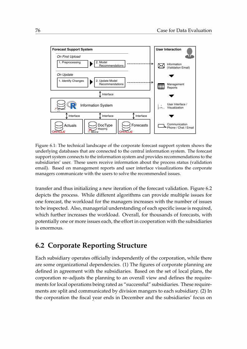
76 Case for Data Evaluation
Information System!
Forecast Support System! User Interaction!
Actuals!!
DocType Mapping!
Forecasts!!
Information!(Validation Email)!
User Interface / Visualization!
Communication Phone / Chat / Email!
1. Preprocessing !
2. Model Recommendations!
On Update!
1. Identify Changes!
2. Update Model Recommendations! Management
Reports!
On First Upload!
Interface! Interface!Interface!
Interface!
Figure 6.1: The technical landscape of the corporate forecast support system shows theunderlying databases that are connected to the central information system. The forecastsupport system connects to the information system and provides recommendations to thesubsidiaries’ user. These users receive information about the process status (validationemail). Based on management reports and user interface visualizations the corporatemanagers communicate with the users to solve the recommended issues.
transfer and thus initializing a new iteration of the forecast validation. Figure 6.2depicts the process. While different algorithms can provide multiple issues forone forecast, the workload for the managers increases with the number of issuesto be inspected. Also, managerial understanding of each specific issue is required,which further increases the workload. Overall, for thousands of forecasts, withpotentially one or more issues each, the effort in cooperation with the subsidiariesis enormous.
6.2 Corporate Reporting Structure
Each subsidiary operates officially independently of the corporation, while thereare some organizational dependencies. (1) The figures of corporate planning aredefined in agreement with the subsidiaries. Based on the set of local plans, thecorporation re–adjusts the planning to an overall view and defines the require-ments for local operations being rated as “successful” subsidiaries. These require-ments are split and communicated by division mangers to each subsidiary. (2) Inthe corporation the fiscal year ends in December and the subsidiaries’ focus on

Case for Data Evaluation 77
Subsidiary! Corporation!
Start!
End!
changes needed?!
yes! no!
data acquisition and preparation!
update forecasts!
data transfer! syntax validation!
semantic validation!
recommend inspection!
manual review!
finalize!
Figure 6.2: The validation process for the delivered forecast data of the subsidiary. Theprocess is starts with the initialize data acquisition preparation of the subsidiary. Afterthe data transfer the data is processed within the information and forecast support sys-tem that validates the data and recommends specific forecasts for inspection. Corporatemanagers manually review the forecast data and can iterate a new forecast update or canfinalize the process.
meeting targets is assumed to be most pronounced at the end of the year. (3) Inevery subsidiary, a manager dedicated to forecasting should provide accurateforecasts to the best of his knowledge for the corporation. The corporation doesnot incentivize the managers for these tasks. (4) Full time employees in the sub-sidiaries are expected to work on a mix of different tasks, if the workload in plan-ning, forecasting, or operations enables resource shifts. (5) As the subsidiaries op-erate independently, they have their own financial system and a heterogeneouspayment structure (e.g., incentivization bonuses), and they have to ensure liq-uidity for their operations (e.g., with earnings management processes). (6) Eachsubsidiary that is participating in the forecasting process –mostly large-volumeentities– enters their expectations on future cash flow in a digital, corporate–based forecasting system. Forecasts accessible are aggregated for corporate riskmanagement to apply hedging measures and further instruments later on.
Figure 6.3 depicts the interactions between the corporation and a subsidiary.Planning figures, forecasts, and realization volumes are needed to be communi-cated, but the responsible managers (planner, forecaster, and earnings manager)
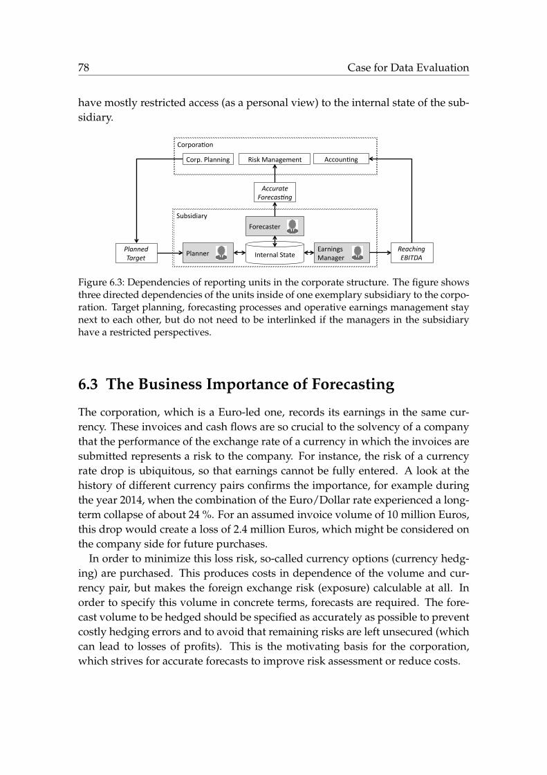
78 Case for Data Evaluation
have mostly restricted access (as a personal view) to the internal state of the sub-sidiary.
Planner Earnings Manager
Forecaster
Reaching EBITDA
Planned Target Internal State
Subsidiary
Corpora9on
Risk Management Accoun9ng Corp. Planning
Accurate Forecas9ng
Figure 6.3: Dependencies of reporting units in the corporate structure. The figure showsthree directed dependencies of the units inside of one exemplary subsidiary to the corpo-ration. Target planning, forecasting processes and operative earnings management staynext to each other, but do not need to be interlinked if the managers in the subsidiaryhave a restricted perspectives.
6.3 The Business Importance of Forecasting
The corporation, which is a Euro-led one, records its earnings in the same cur-rency. These invoices and cash flows are so crucial to the solvency of a companythat the performance of the exchange rate of a currency in which the invoices aresubmitted represents a risk to the company. For instance, the risk of a currencyrate drop is ubiquitous, so that earnings cannot be fully entered. A look at thehistory of different currency pairs confirms the importance, for example duringthe year 2014, when the combination of the Euro/Dollar rate experienced a long-term collapse of about 24 %. For an assumed invoice volume of 10 million Euros,this drop would create a loss of 2.4 million Euros, which might be considered onthe company side for future purchases.
In order to minimize this loss risk, so-called currency options (currency hedg-ing) are purchased. This produces costs in dependence of the volume and cur-rency pair, but makes the foreign exchange risk (exposure) calculable at all. Inorder to specify this volume in concrete terms, forecasts are required. The fore-cast volume to be hedged should be specified as accurately as possible to preventcostly hedging errors and to avoid that remaining risks are left unsecured (whichcan lead to losses of profits). This is the motivating basis for the corporation,which strives for accurate forecasts to improve risk assessment or reduce costs.

Case for Data Evaluation 79
6.4 Domain Expert Knowledge
In reconciliation with the management of the sample corporation, I used a datadriven approach to identify several issues for the data base. The approachled to identification of issues that are explainable and covered by expert’s do-main knowledge, and those issues that required interaction with the subsidiaries.These aforementioned issues cover the following topics:
Issues covered by Expert Knowledge
(1) Very few samples of a testing entity are inside of the database. These samplesmust be removed as they exhibit irrelevant data of forecasts and actuals. (2) Dueto the system requirements, data samples of the holding corporation is containedinside of the database. The data is required to be removed. (3) Data samplesof entities that are from Argentina encounter political import and export restric-tions. The data samples are required to be removed. (4) Subsidiaries can switchinvoice currencies due to business decisions. As the human forecaster does ordoes not know about this situation, the forecasts can entail very high errors. Acurrency switch can occur in one step or over a longer period of time with partialadjustments for invoice items. For instance, switching the realization currencycompletely from the symbolic old currency A to the new currency B in one stepcan result in forecasts being unaligned to this matter. This results in all fore-casts of one specific invoice item having no actual counterpart in currency A andup to five forecasts entail a percentage error of −100.0 % when the forecasts arerevised. Additionally, the second currency B misses the forecasts which resultsin five additional forecast errors. This will result in a high percentage error independence to the other invoice volumes in that currency B. Currency switchesusually apply in more than one single month. These currency switches starts ata specific point in time and items are issued and received with the new currencyin the period after. This may result in up to 15 forecast series being associatedto the wrong currency, depending on the time the forecaster receives informationfor the currency switch. In total, each single currency switch can have a massiveimpact on error metrics for up to 150 forecasts. Possible solutions are to removeor recalculate the respective items. In reconciliation with the sample company,the items in both currencies are recalculated in the EUR currency, for both fore-casts and actuals. This enables identification of overalls-errors for forecasts. But,as a result, the specific items must be recalculated to the original currencies whenhedging measures are applied. (5) Usually the standardized three letter currencycode should be provided for forecasts and actuals. But, the currencies of items

80 Case for Data Evaluation
were not standardized in the beginning working period of the information sys-tem. Data items with misspelled currencies and currency codes like “097” dooccur. Data samples of these issues have to be removed, as an allocation is notpossible. (6) For the American subsidiaries five so called reference entities exist.These entities provide aggregate forecasts of the other subsidiaries in the USAwith regard to the different business divisions. The actuals of each subsidiaryin USA are provided separately. But, some subsidiaries do not deliver actualrealization volumes – mostly small entities. In reconciliation with the manage-ment of the sample corporation, the data samples should be removed. (7) Asrealization entries are made by humans, sometimes false booking entries for ac-tuals do exist. The mistaken entries are corrected with a second booking for thatitem with the inverse signed volume. As these mistakes are recognized mostlyin the same month there is nearly no effect. Very few corrections have a delaythat result in corrections being shifted in the next, or later months. These correc-tion entries are easy to identify based on the exact volume and inverse sign andshould be removed. (8) Subsidiaries exist that are not fully registered in the cor-porate database. This issue results in missing information for local currencies inwhich the subsidiary operates, preventing hedging operations. These data sam-ples should be removed. (9) For twenty-one subsidiaries no technical interfacedoes exist to provide actual realization volumes to the database. For these fore-casts no actual counterpart exists. To prevent percentage errors of−100.0 % thesedata samples must be removed.
Issues Requiring Subsidiary Knowledge
For each forecasting subsidiary, a local database provides actual realization vol-umes for invoices. These booking systems of the subsidiaries have different labelsfor document types, a two letter alphanumeric code system. These codes have de-veloped over the years and their meaning depends on the subsidiaries. Thus, thesame document code can provide different meanings for different subsidiaries.Furthermore, the subsidiary’s document codes depend in few special cases oncurrencies, partner subsidiary, and time of the invoice.
Based on these attributes, I developed a classification system that allocates thespecific invoice type by a combination of attribute characteristics (classificationtuple). If the classification does not allocate an item type, the item is dismissedin the further analyses and the classification frames the item type as “unknown”.The classification tuple is described in Equation 6.1.
ItemType = (Document Type, Subsidiary, Partner, Currency, Date) (6.1)

Case for Data Evaluation 81
The specific characteristics that determine a item type are stored in a centraldatabase within the forecast support system. After my implementation of theclassification system, the corporate manager reconciled with the subsidiaries todetermine the meaning of specific document types, reducing the existing un-known items to a minimum (in volume and number). The specific attribute char-acteristics were updated in the database to provide knowledge for future datadeliveries. Continuous improvement processes were implemented to ensure thevalidity of the classification system.
6.5 Data Preprocessing in Practice
The CRISP-DM reference model (Chapman et al., 1999, p. 10) describes the typicalstages of a data mining process, upon which the data mining process was buildon. In practice, the preprocessing of the data mining process for development ofthe forecast support system in the sample corporation requires data acquisition,data understanding, and the identification of foretold data artifacts. Further workis required for the classification system, establishing continuous improvementprocesses, and in acquisition a comprehensive business understanding. The dataacquisition, data understanding, and preprocessing is widely known to take up to80 % of the total workload for data mining processes (Mannila, 1996). The amountof work in my project with the corporation did take about 3.0 years for thesesteps and around 75 % of the initial workload. This workload does not cover thesoftware implementation of the data classification and continuous improvementprocesses. The data cleaning process covers the applied steps of “PreprocessingContent Cleaning” and “Preprocessing Ratio Cleaning”, to provide high qualityinput for the scientific analyses. The section “Preprocessing Overview” providesan overview on the metrics for different stages of data preprocessing.
Preprocessing Content Cleaning
The data cleaning covers the following preprocessing steps: (1) Integration of allconsiderable and known issues retrieved by expert knowledge and subsidiaryknowledge. The data samples are removed or recalculated as exhibited previ-ously. (2) Removing samples that contain false sign of invoice type. For instance,items of type “invoice received” that have a forecast or actual above zero states afalse direction of invoice flow. (3) Samples with an actual monthly volume below100,000 EUR equivalent will to be removed due to a high expected percentage er-ror. (4) Removing samples that exhibit a percentage error of more than 1,500.0 %.

82 Case for Data Evaluation
Preprocessing Ratio Cleaning
After the cleaning based on expert and content knowledge, further preprocessingbased on ratio insights is applied. These steps of preprocessing cover: (1) Sam-ples that miss one item type of invoices in forecasts or actuals are removed, as aratio can not be obtained without the complement of item type. (2) Subsidiariesthat permanently have a ratio level of zero are removed, as these result mostlyfrom selling-only subsidiaries. In such cases a normalization is not possible.(3) Removing samples that have a ratio above five, as these result mostly fromselling-only subsidiaries. (4) Samples that have a history of less then four yearsare removed to ensure both target calculation over three years and out-of-sampleevaluation of one year. (5) Ratios of currencies that do not achieve a correla-tion over 0.8 to the overall ratio of a subsidiary are filtered. The intention is thatcurrencies without high correlation to the subsidiaries ratio can hardly providehedging opportunities without further correction, which would require an ap-proach based on the split of invoice received and issued depending on all entityspecific currency.
Preprocessing Overview
Table 6.2 shows the different stages of preprocessing. Mean percentage error forthe whole data set (second column) is reduced from nearly 80,000.0 % down to51.4 % for the content cleaning and down to 28.5 % for ratio cleaning. Medianpercentage errors are reduced too. Obviously, these numbers state that cleaningis essential for data analyses and predictive purposes. With poorly preprocessedor unprocessed data the predictive models and analyses will render unreliable.

Case
forD
ataEvaluation
83
Metric Data Sample
ape All AP HP IM DV EUR USD
Pseudo Actuals (Data #0)
mean 58.7 % 84.2 % 44.4 % 55.3 % 90.2 % — 542.2 %
median — — — — — — —
Uncleaned (Data #1)
mean 79237.8 % 414.0 % 1900.5 % 8316.7 % 186399.6 % 1465.3 % 2696.1 %
median 84.8 % 98.8 % 58.6 % 100.0 % 100.0 % 60.3 % 77.9 %
Content Cleaned (Data #2)
mean 51.4 % 55.8 % 44.3 % 47.7 % 44.0 % 42.6 % 58.4 %
median 26.1 % 33.8 % 24.5 % 26.8 % 24.5 % 19.0 % 29.9 %
Ratio Cleaned (Data #3)
mean 28.5 % 44.7 % 27.2 % 21.5 % 24.4 % 14.4 % 35.2 %
median 12.8 % 17.8 % 9.2 % 12.6 % 12.5 % 8.7 % 19.3 %
Table 6.2: Importance of data cleaning: Comparison of ape metric for different stages of uncleaned and cleaned data. First columnnotates if mean and median of the ape metric taken. The other columns cover numbers for the whole dataset, all divisions, andselected currencies. Data #0 show numbers as reported in (Martin, 2012), but just covers deliveries of 06/2009 to 11/2010 anddoes not cover median metric and EUR. His numbers do not cover ape based on real actuals, instead pseudo-actuals are taken(pseudo-actuals replace actuals A(i) by forecasts 1F(i) and use the second to last forecasts instead of the last ones (1F(i) := 2F(i)).Data #1 is the raw, uncleaned data. Data #2 is derived from Data #1 and applies preprocessing for content cleaning – the data isused in the individual analyses of this thesis. Data #3 additionally applies preprocessing for ratio cleaning. The resulting data isused in the ratio analyses of this thesis.
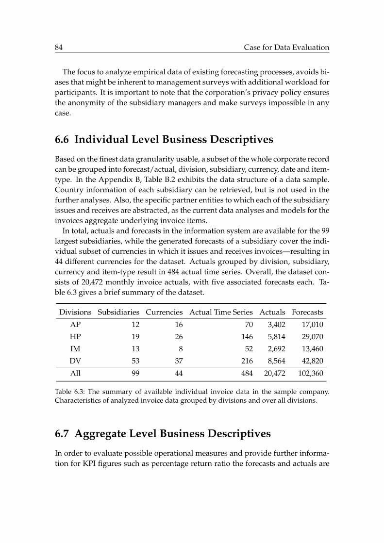
84 Case for Data Evaluation
The focus to analyze empirical data of existing forecasting processes, avoids bi-ases that might be inherent to management surveys with additional workload forparticipants. It is important to note that the corporation’s privacy policy ensuresthe anonymity of the subsidiary managers and make surveys impossible in anycase.
6.6 Individual Level Business Descriptives
Based on the finest data granularity usable, a subset of the whole corporate recordcan be grouped into forecast/actual, division, subsidiary, currency, date and item-type. In the Appendix B, Table B.2 exhibits the data structure of a data sample.Country information of each subsidiary can be retrieved, but is not used in thefurther analyses. Also, the specific partner entities to which each of the subsidiaryissues and receives are abstracted, as the current data analyses and models for theinvoices aggregate underlying invoice items.
In total, actuals and forecasts in the information system are available for the 99largest subsidiaries, while the generated forecasts of a subsidiary cover the indi-vidual subset of currencies in which it issues and receives invoices—resulting in44 different currencies for the dataset. Actuals grouped by division, subsidiary,currency and item-type result in 484 actual time series. Overall, the dataset con-sists of 20,472 monthly invoice actuals, with five associated forecasts each. Ta-ble 6.3 gives a brief summary of the dataset.
Divisions Subsidiaries Currencies Actual Time Series Actuals Forecasts
AP 12 16 70 3,402 17,010
HP 19 26 146 5,814 29,070
IM 13 8 52 2,692 13,460
DV 53 37 216 8,564 42,820
All 99 44 484 20,472 102,360
Table 6.3: The summary of available individual invoice data in the sample company.Characteristics of analyzed invoice data grouped by divisions and over all divisions.
6.7 Aggregate Level Business Descriptives
In order to evaluate possible operational measures and provide further informa-tion for KPI figures such as percentage return ratio the forecasts and actuals are

Case for Data Evaluation 85
aggregated for the corporate risk management. As a proxy for the percentage re-turn margin within a fiscal year, the entity’s ratio of aggregated revenues (II) andexpenses (IR) is calculated. The aggregated dataset used in the analysis coversforecasts and actual for the entities’ ratios.
In total, actuals and forecasts are available for the 67 largest subsidiaries result-ing in 25 different currencies for the dataset. Actuals grouped by division, sub-sidiary, currency and item-type result in 72 actual time series. Overall, the datasetconsists of 3,087 monthly invoice actuals, with five associated forecasts each. Theunderlying raw dataset of non-aggregated forecasts cover 102,360 items. Table 6.4gives a brief summary of the ratio dataset.
Divisions Subsidiaries Currencies Actual Time Series Actuals Forecasts
AP 10 7 11 618 3,090
HP 13 8 15 608 3,040
IM 6 4 7 420 2,100
DV 38 20 39 1,441 7,205
All 67 25 72 3,087 15,435
Table 6.4: The summary of available aggregate invoice data in the sample company. Char-acteristics of analyzed invoice ratio data grouped by divisions and over all divisions.
Additionally, partial data from the official corporation’s annual report are usedfor testing the hypotheses. In the annual report 2010 the EBITDA margins listedare 19.0 % (AP), 26.0 % (HP), and 13.4 % (IM). Official figures for division DVwere not reported separately. In 2011, the figures were: 22.8 % (AP), 27.4 % (HP),and 10.8 % (IM). In 2012, the figures were: 24.0 % (AP), 27.2 % (HP), and 10.9 %(IM). The figures in 2013 were comparable in magnitude, namely, 25.5 % (AP),28.2 % (HP), and 9.5 % (IM).
6.8 Framework for Data Evaluation
These analyses for the data evaluation uses several techniques to retain the em-pirical results. These analyses consist of methods, such as correlation analysisfor efficiency, linear regression analysis, in particular revision and error analysis,analysis of the out-of-sample results, and t-test evaluation. For the analyses andhypothesis testing the experiments use the programming language R and toolsprovided by (R Core Team, 2013) and the libraries corrplot (Wei and Simko,2016), data.table (Dowle et al., 2015), and ggplot2 (Wickham et al., 2016).

Chapter 7
Evaluation of Individual LevelCharacteristics
The following sections analyze the sample data set (see Table 6.3) for indi-vidual level forecasts and present the empirical results of the analyses from
Chapter 3. These results cover efficiency analyses, testing of the efficiency hy-pothesis, and the analyses of individual level biases. The results are followed bythe interpretation and a final summary.
7.1 Forecasting Efficiency
The Propositions (P1) and (P2) for weak forecast efficiency are tested by exam-ining correlations between forecast errors and revisions as well as between revi-sions. The first four columns of Table 7.1 show Spearman correlations betweenrelative revisions and percentage errors. The last three columns of Table 7.1show Spearman correlations between relative revisions. Significance levels of thep-values are given after the correlation value.
87

88Evaluation
ofIndividualLevelCharacteristics
Proposition 1 Proposition 2
4pe 3pe 2pe 1pe 3r 2r 1r
4r −0.04 ∗∗∗ −0.04 ∗∗∗ −0.06 ∗∗∗ −0.05 ∗∗∗ 0.07 ∗∗∗ 0.08 ∗∗∗ −0.03 ∗∗
3r −0.01 −0.04 ∗∗∗ −0.07 ∗∗∗ 0.11 ∗∗∗ 0.09 ∗∗∗
2r −0.03 ∗∗ −0.03 ∗∗ 0.04 ∗∗∗
1r −0.08 ∗∗∗
Note: ∗p<0.1; ∗∗p<0.05; ∗∗∗p<0.01
Table 7.1: Spearman correlations and significance levels of percentage error and relative revision. The correlations are groupedbased on Nordhaus Propositions 1 & 2. Significant correlations indicate inefficient individual level forecasting. The results showthat revisions (tr) are inefficient for errors τ pe (Proposition 1) and revisions τr (Proposition 2) at all times.

Evaluation of Individual Level Characteristics 89
All but one of the correlations are significant with p-values below 0.05. With es-timated correlation coefficients between−8 % and−1 %, all correlations betweenforecast errors and revisions are negative and relatively small. Correlations be-tween revisions are positive except for the correlation between revisions 1r and 4r.The results indicate violation of both Propositions. The revisions 1r and 4r com-prise forecasts of different years (1F and 5F), wherefore their negative correlationmight exhibit a interesting conjunction to the year in which the forecast are made.This suggests that the corporation’s forecasting processes are not weak efficient.
7.1.1 Forecast Efficiency: Lead Time
Next, the analyses focuses on how inefficiencies are related to forecast accuracy.Proposition (P3) suggests that forecasts are less accurate when they are inefficient.In other words, Proposition (P3) leads to the expectation that forecast accuracylessens with the strength of inefficiency patterns – in the revision setting, as leadtimes shorten. Analysis covers forecast groups separated by division and fordifferent lead times.
Results in Tables 7.2 and 7.3 show mape values by lead time and division for allmonths (Table 7.2) and for December actuals only (Table 7.3). Taking all monthstogether, it’s observable that mape generally decreases with lead time. The excep-tion is an increase between 4F and 3F in division AP. Taking December forecastsonly, increasing mape is observable between 2F and 1F for divisions AP and IM,and between 3F and 2F for DV and IM.
Division Lead time (in Quarters)
t = 5 t = 4 t = 3 t = 2 t = 1
AP 0.655 0.582 0.594 0.566 0.558HP 0.543 0.490 0.477 0.472 0.443IM 0.579 0.530 0.517 0.493 0.477DV 0.570 0.486 0.466 0.457 0.440
Table 7.2: Mean absolute percentage error (mape) by division for all months. Most divi-sions have decreasing errors for decreasing lead time and are aligned to theory, exceptfor division AP (from lead time t = 4 to t = 3).
The findings show that a decrease of the lead time is not associated with areduction of the error. This provides the first indication that some influences areat play and Proposition (P4) may not hold.

90 Evaluation of Individual Level Characteristics
Division Lead time (in Quarters)
t = 5 t = 4 t = 3 t = 2 t = 1
AP 0.784 0.723 0.699 0.675 0.724HP 0.603 0.562 0.553 0.543 0.526IM 0.649 0.542 0.503 0.523 0.559DV 0.639 0.549 0.508 0.524 0.503
Table 7.3: Mean absolute percentage error (mape) by division for December. Divisionshave decreasing errors, except in divisions AP (from lead time t = 2 to t = 1), in divisionIM (from lead time t = 3 to t = 2, to t = 1), and in division DV (from lead time t = 3 tot = 2), where the mape increases for these forecast revisions. The results for these threedivisions are contrary to theory.
7.1.2 Forecast Efficiency Hypothesis: Increased Accuracy
For Proposition 4 the analyses cover the relation of mape(1F) to the absolutecorrelation values |Cor(x, y)| of all Nordhaus’s correlations that are derived onan entity–currency level. Table 7.4 shows the results of bivariate correlationtests on mape(1F) and absolute correlations between revisions and percentageerrors (|Cor(tr, τ pe)|), and on mape(1F) and absolute correlations between revi-sions (|Cor(tr, τr)|). The first ten rows in Table 7.4 show the correlations betweenmape and absolute correlations between revisions and percentage errors. Propo-sition (P4) holds for one case (|Cor(3r, 1pe)|). In two cases, |Cor(1r, 1pe)| and|Cor(3r, 3pe)|, inefficiency patterns are associated with higher forecast accuracy(rejection of Proposition (P4)). The next six rows in Table 7.4 show correlations be-tween mape and absolute correlations between revisions. Proposition (P4) againholds for one case (|Cor(4r, 3r)|). In two cases, |Cor(2r, 1r)| and |Cor(3r, 1r)|, in-efficiency patterns are associated with higher accuracy. For each single estimatemore than 1,400 absolute correlation values |Cor(x, y)| were accessed, which un-derlines the significance of the results.
In summary, obtained results are mixed for Proposition (P4). Two correlationsshow that efficient forecasting is associated with lower error levels – while fourcorrelations show contrary results. I conclude that inefficient forecasts are notnecessarily associated with lower forecast accuracy – counter-intuitively, someinefficiency patterns are even associated with higher accuracy. This thesis com-plements the literature with a study where revision patterns are associated withhigher forecast accuracy, that is why Proposition (P4) is not supported. Therefore,the validity of the efficiency hypothesis must be refused for the analyzed data ofcorporate internal forecasts, which supports Hypothesis 1.
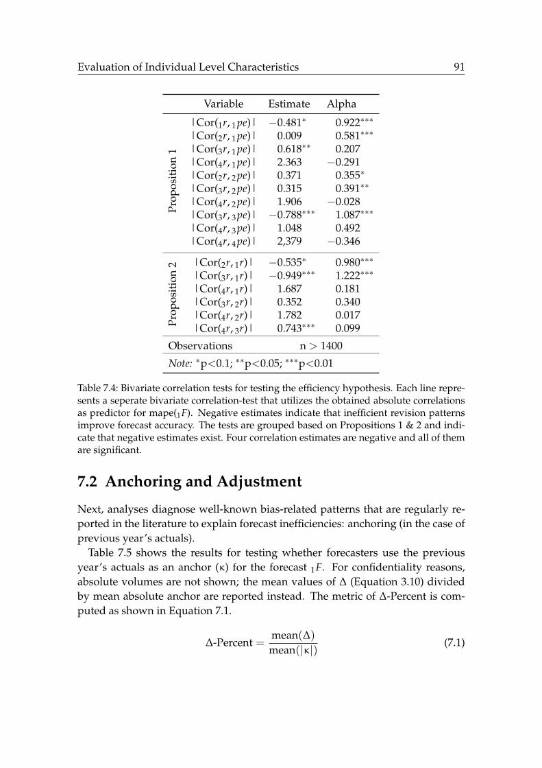
Evaluation of Individual Level Characteristics 91
Variable Estimate Alpha
Prop
osit
ion
1
|Cor(1r, 1pe)| −0.481∗ 0.922∗∗∗
|Cor(2r, 1pe)| 0.009 0.581∗∗∗
|Cor(3r, 1pe)| 0.618∗∗ 0.207|Cor(4r, 1pe)| 2.363 −0.291|Cor(2r, 2pe)| 0.371 0.355∗
|Cor(3r, 2pe)| 0.315 0.391∗∗
|Cor(4r, 2pe)| 1.906 −0.028|Cor(3r, 3pe)| −0.788∗∗∗ 1.087∗∗∗
|Cor(4r, 3pe)| 1.048 0.492|Cor(4r, 4pe)| 2,379 −0.346
Prop
osit
ion
2 |Cor(2r, 1r)| −0.535∗ 0.980∗∗∗
|Cor(3r, 1r)| −0.949∗∗∗ 1.222∗∗∗
|Cor(4r, 1r)| 1.687 0.181|Cor(3r, 2r)| 0.352 0.340|Cor(4r, 2r)| 1.782 0.017|Cor(4r, 3r)| 0.743∗∗∗ 0.099
Observations n > 1400
Note: ∗p<0.1; ∗∗p<0.05; ∗∗∗p<0.01
Table 7.4: Bivariate correlation tests for testing the efficiency hypothesis. Each line repre-sents a seperate bivariate correlation-test that utilizes the obtained absolute correlationsas predictor for mape(1F). Negative estimates indicate that inefficient revision patternsimprove forecast accuracy. The tests are grouped based on Propositions 1 & 2 and indi-cate that negative estimates exist. Four correlation estimates are negative and all of themare significant.
7.2 Anchoring and Adjustment
Next, analyses diagnose well-known bias-related patterns that are regularly re-ported in the literature to explain forecast inefficiencies: anchoring (in the case ofprevious year’s actuals).
Table 7.5 shows the results for testing whether forecasters use the previousyear’s actuals as an anchor (κ) for the forecast 1F. For confidentiality reasons,absolute volumes are not shown; the mean values of ∆ (Equation 3.10) dividedby mean absolute anchor are reported instead. The metric of ∆-Percent is com-puted as shown in Equation 7.1.
∆-Percent =mean(∆)mean(|κ|) (7.1)

92 Evaluation of Individual Level Characteristics
In nine months patterns are observed that fit anchoring (negative ∆-Percent).In five of those months the effect is significant to the p-value of 0.05, and it is par-ticularly pronounced (∆-Percent = −0.06, p < 0.001) in the last two months ofa year. This intensified A&A effect at the end of the year suggests that previousyear’s actual is much more important for the expert’s forecasts. A predeterminedbusiness objective that has to be achieved at the end of a business cycle and there-fore anchors forecasts would correspond to these circumstances.
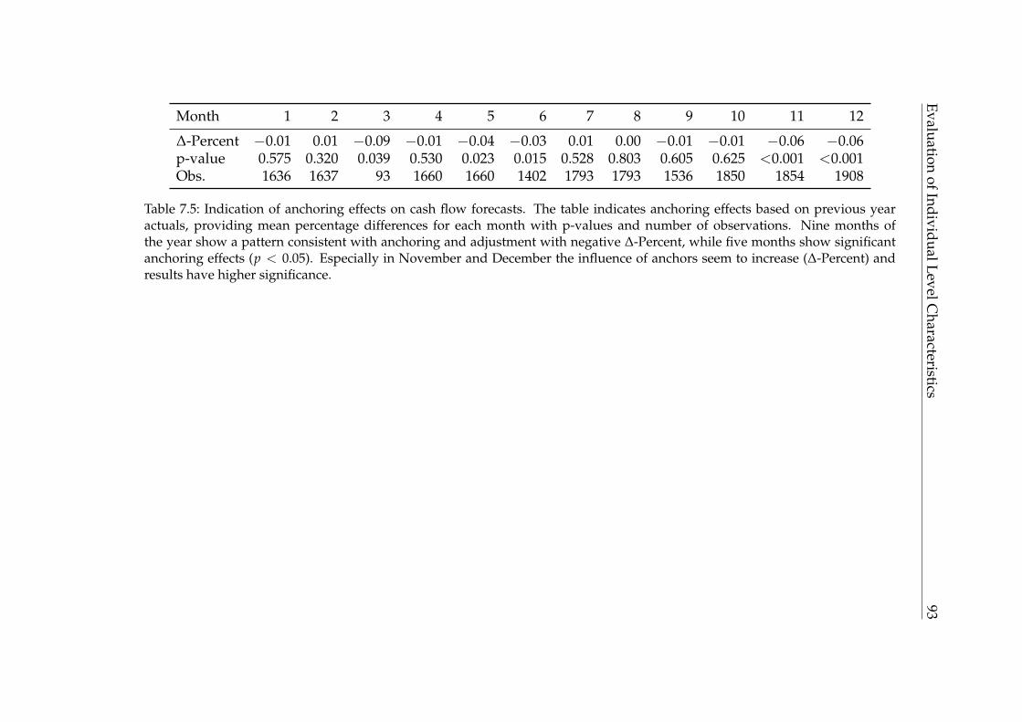
EvaluationofIndividualLevelC
haracteristics93
Month 1 2 3 4 5 6 7 8 9 10 11 12
∆-Percent −0.01 0.01 −0.09 −0.01 −0.04 −0.03 0.01 0.00 −0.01 −0.01 −0.06 −0.06p-value 0.575 0.320 0.039 0.530 0.023 0.015 0.528 0.803 0.605 0.625 <0.001 <0.001Obs. 1636 1637 93 1660 1660 1402 1793 1793 1536 1850 1854 1908
Table 7.5: Indication of anchoring effects on cash flow forecasts. The table indicates anchoring effects based on previous yearactuals, providing mean percentage differences for each month with p-values and number of observations. Nine months ofthe year show a pattern consistent with anchoring and adjustment with negative ∆-Percent, while five months show significantanchoring effects (p < 0.05). Especially in November and December the influence of anchors seem to increase (∆-Percent) andresults have higher significance.
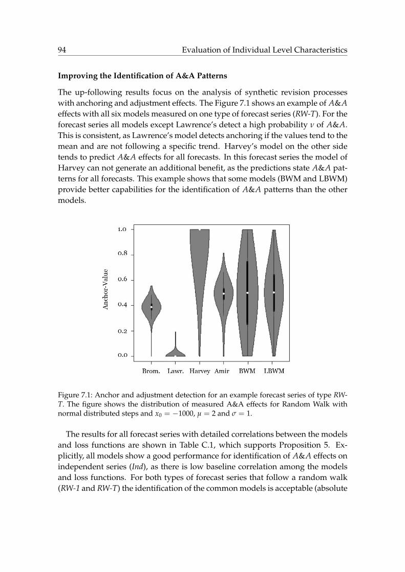
94 Evaluation of Individual Level Characteristics
Improving the Identification of A&A Patterns
The up-following results focus on the analysis of synthetic revision processeswith anchoring and adjustment effects. The Figure 7.1 shows an example of A&Aeffects with all six models measured on one type of forecast series (RW-T). For theforecast series all models except Lawrence’s detect a high probability ν of A&A.This is consistent, as Lawrence’s model detects anchoring if the values tend to themean and are not following a specific trend. Harvey’s model on the other sidetends to predict A&A effects for all forecasts. In this forecast series the model ofHarvey can not generate an additional benefit, as the predictions state A&A pat-terns for all forecasts. This example shows that some models (BWM and LBWM)provide better capabilities for the identification of A&A patterns than the othermodels.
Figure 7.1: Anchor and adjustment detection for an example forecast series of type RW-T. The figure shows the distribution of measured A&A effects for Random Walk withnormal distributed steps and x0 = −1000, µ = 2 and σ = 1.
The results for all forecast series with detailed correlations between the modelsand loss functions are shown in Table C.1, which supports Proposition 5. Ex-plicitly, all models show a good performance for identification of A&A effects onindependent series (Ind), as there is low baseline correlation among the modelsand loss functions. For both types of forecast series that follow a random walk(RW-1 and RW-T) the identification of the common models is acceptable (absolute
Evaluation of Individual Level Characteristics 95
correlation values above those of Ind). For RW-1, all models show a correlationin dependence to the loss function between 0.22 and 0.50, while the model ofLawrence reached a value between −0.10 and −0.20. Bromiley’s model performsquite good, but reached lower correlation values than both Bandwidth Modelsfor random walk series. The Bandwidth Models identify the A&A pattern in areliable way and outperform the other models by far for either loss function. Thisis mainly a result of the fact that both models are taking all values into account,but are not as easily influenced by small changes as the other approaches. Addinga trend (RW-T series) enhances all correlation values of the models further. In thisseries, LBWM is able to reach a correlation of 0.67 with the RMSE closely followedby BWM with 0.60 and Bromiley’s model with only 0.40. In all three series theresults of Lawrence’s model are strictly dominated by the other models, which isreasonable as the used series do not tend to the mean. For these first three forecastseries both Bandwidth Models show a good performance compared to the othermodels. The performance differs especially for the growth series LogG and ExpG,where correlations decrease. Detection of A&A effects seems to be more difficult.For strict monotone growth series the N.A.s describe that Harvey’s model alwaysdetects A&A and Lawrence’s never detects A&A. No correlation is be calculatedfor Amir’s model for LogG series as it is resulting in either 1 or 0. Thereforenone will be further considered for these forecast series. However, the Band-width Models show an good precision in detecting A&A effects for these seriesand are highly correlated with the used loss function in general. An overview ofthe comparison is shown in Table 7.6.
To further improve the precision of identification for these particular growthseries (LogG and ExpG) one could transform the forecast series with the inversefunction: the exponential function for LogG series and the logarithmic functionfor ExpG series. Another possibility would be to modify the model directly by acorresponding function, e. g. to use bandwidths for exponential growth insteadof percentage growth in an area where BWMs perform best.
Proposition 6 suggests that the the degree of A&A identification of the modelscorrelate with one another, in dependence to the forecast series. The Pearson cor-relation coefficient is used for the correlation between the different models. A lowcorrelation for a forecast series will state that a combination of different modelswould be beneficial for identification of A&A effects. The correlations betweenthe models are shown in Table C.2, which supports Proposition 6. For Bromi-ley’s model the correlation to the other models highly depends on the kind offorecast series. For instance, in the ExpG series Bromiley’s model and the Band-width Models have instead of a high positive correlation a low negative corre-lation of −0.1, reasoned by the separate treatment of positive and negative revi-

96 Evaluation of Individual Level Characteristics
Model Time Series
Ind RW-1 RW-T LogG ExpG
Bromiley√ √ √
© ©Lawrence
√ √ √N.A. N.A.
Harvey√ √ √
N.A. N.A.Amir
√ √ √N.A. ©
BWM√ √√ √√
© ©LBWM
√ √√ √√© ©
Appropriate Use: © with limitations,√
good,√√
better.
Table 7.6: Comparison of A&A models on different time series.
sions by Bromiley’s model. The approach of Lawrence focuses on the mean of theprevious forecast instead of tendencies, which results in low or even negative cor-relations with the other approaches. The models of Lawrence and Harvey shownegative correlation, but both models can not be considered for the forecast seriesof LogG and ExpG. Lawrence’s model never detects A&A and Harvey’s model al-ways does. Furthermore, Harvey’s and Amir’s models show a high correlation,as both are considering if consecutive revisions dispose over equal signs. Amir’smodel is not considered for LogG, as the resulting values are only 0 and 1. Finally,a very high correlation was found between BWM and LBWM, consistent over allkinds of series.
Combining multiple models can be an appropriate approach if the models arehighly correlated with the loss function but not with each other. For instance,Amir’s model is only weak correlated with the Bandwidth Models and all ofthem reach a good correlation with the loss functions. Bromiley on the otherside shows a considerable correlation with all metrics, in dependence to the fore-cast series. As a result, this would suggest that a combination of Amir’s modeland the LBWM can be considered beneficial for A&A identification – especiallywhen combined with a model that accounts for the interaction of forecast serieswith Bromiley’s model.
Interim Result
The results indicate that previous year actual provides an anchor for the sub-sidiary’s forecasting. Especially in the end of the year (November and December)the anchor had highly significant influence on the forecasts. These results suggest

Evaluation of Individual Level Characteristics 97
that cash realizations at the end of the year may have a stronger impact than inthe previous months, and a end-of-year effect may exist.
The results present the Bandwidth Models BWM and LBWM to determineA&A effects. These models are compared with the models from findings of pre-vious papers. The two models base on the A&A influence of previous forecastsfor the succeeding forecast value. The evaluation uses short, synthetic forecastsseries with specific pattern. The Bandwidth Models can predict the probabilityof a forecast series being influenced by A&A effects with higher accuracy andoutperform each analyzed A&A models in at least three types of synthetic timeseries. Detecting the influence of A&A on human forecasters offers high potentialfor forecast correction as they have a higher relation to common loss functions,which supports Proposition 5. For instance, a forecast correction model may beapplied only on those forecasts that exhibit A&A behavior, or even use the infor-mation directly within the correction model to improve the forecast error.
For application of the models it is assumed that real world forecast series havesimilarities to the used kinds of forecast series. The performance of the A&Amodels is expected to partially relate to the real world time series, depending onthe distribution to the patterns of the synthetic forecast series. The applicationon real world series requires further analysis, where the authors of (Knöll andRoßbach, 2018a) started to explore this branch of research.
7.3 Optimism, Pessimism and Overreaction,Underreaction
The following results cover the analyses for biases of optimism, pessimism, over-reaction, and underreaction. Table 7.7 shows outcomes of linear regressions onthe full data set, grouped by revision sign and lead time. Positive revisions arepresented in the first four columns, negative revisions in the last four columns.
In accord with the findings reported by Amir and Ganzach (1998), the resultsindicate the presence of individual biases. For negative revisions, pessimism isobserved: α’s are negative, implying that the actual is, on average, greater thanthe last forecast. For positive revisions, optimism is observed: α’s are positive, im-plying that the actual is, on average, smaller than the last forecast. For both posi-tive and negative revisions, underreaction is observed: β’s are negative, implyingthat revisions are too small. However, contrary to intuition and the findings ofAmir and Ganzach (1998), it is not found that these patterns weaken consistentlyas the forecast horizon shortens. In fact, three of the four patterns become morepronounced; only underreaction in positive forecasts becomes somewhat weaker.
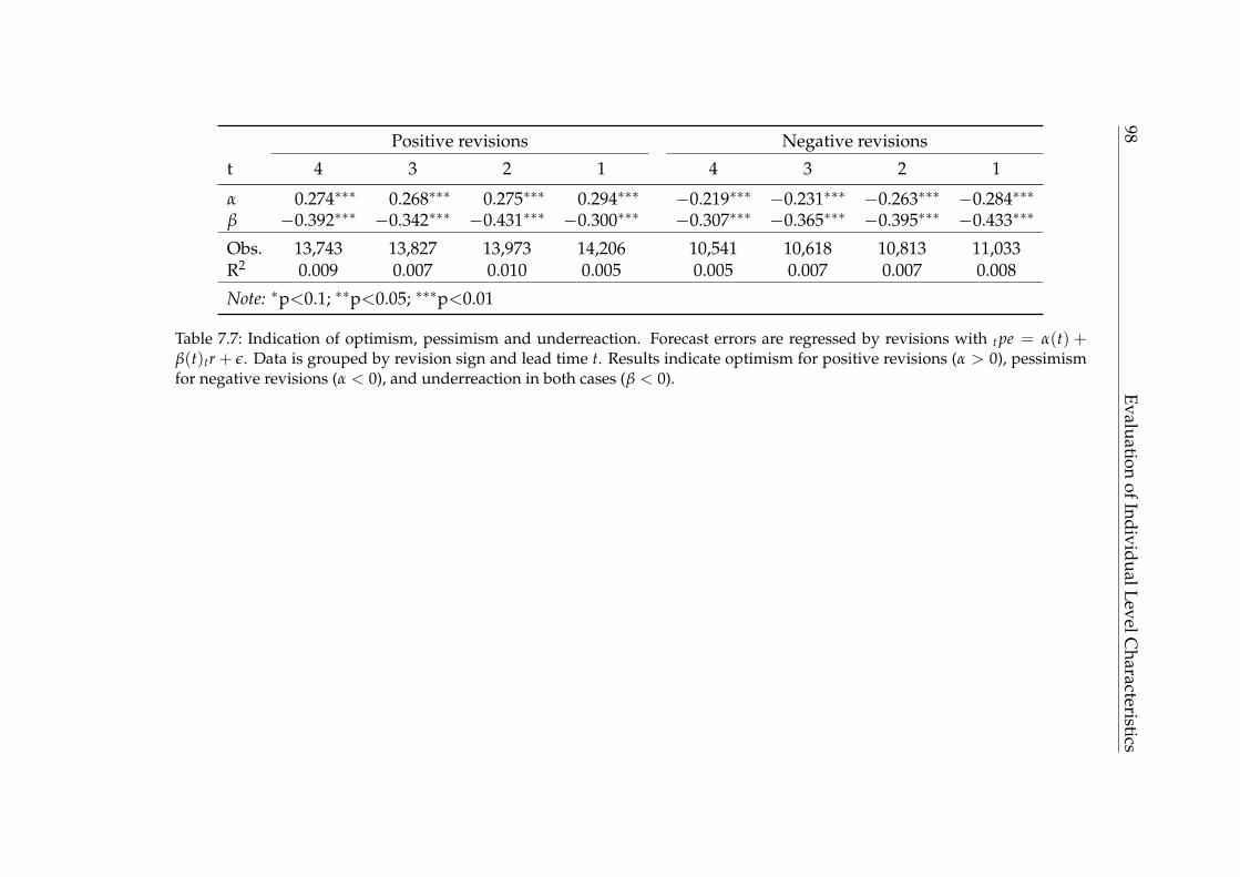
98Evaluation
ofIndividualLevelCharacteristics
Positive revisions Negative revisions
t 4 3 2 1 4 3 2 1
α 0.274∗∗∗ 0.268∗∗∗ 0.275∗∗∗ 0.294∗∗∗ −0.219∗∗∗ −0.231∗∗∗ −0.263∗∗∗ −0.284∗∗∗
β −0.392∗∗∗ −0.342∗∗∗ −0.431∗∗∗ −0.300∗∗∗ −0.307∗∗∗ −0.365∗∗∗ −0.395∗∗∗ −0.433∗∗∗
Obs. 13,743 13,827 13,973 14,206 10,541 10,618 10,813 11,033R2 0.009 0.007 0.010 0.005 0.005 0.007 0.007 0.008
Note: ∗p<0.1; ∗∗p<0.05; ∗∗∗p<0.01
Table 7.7: Indication of optimism, pessimism and underreaction. Forecast errors are regressed by revisions with t pe = α(t) +β(t)tr + ε. Data is grouped by revision sign and lead time t. Results indicate optimism for positive revisions (α > 0), pessimismfor negative revisions (α < 0), and underreaction in both cases (β < 0).
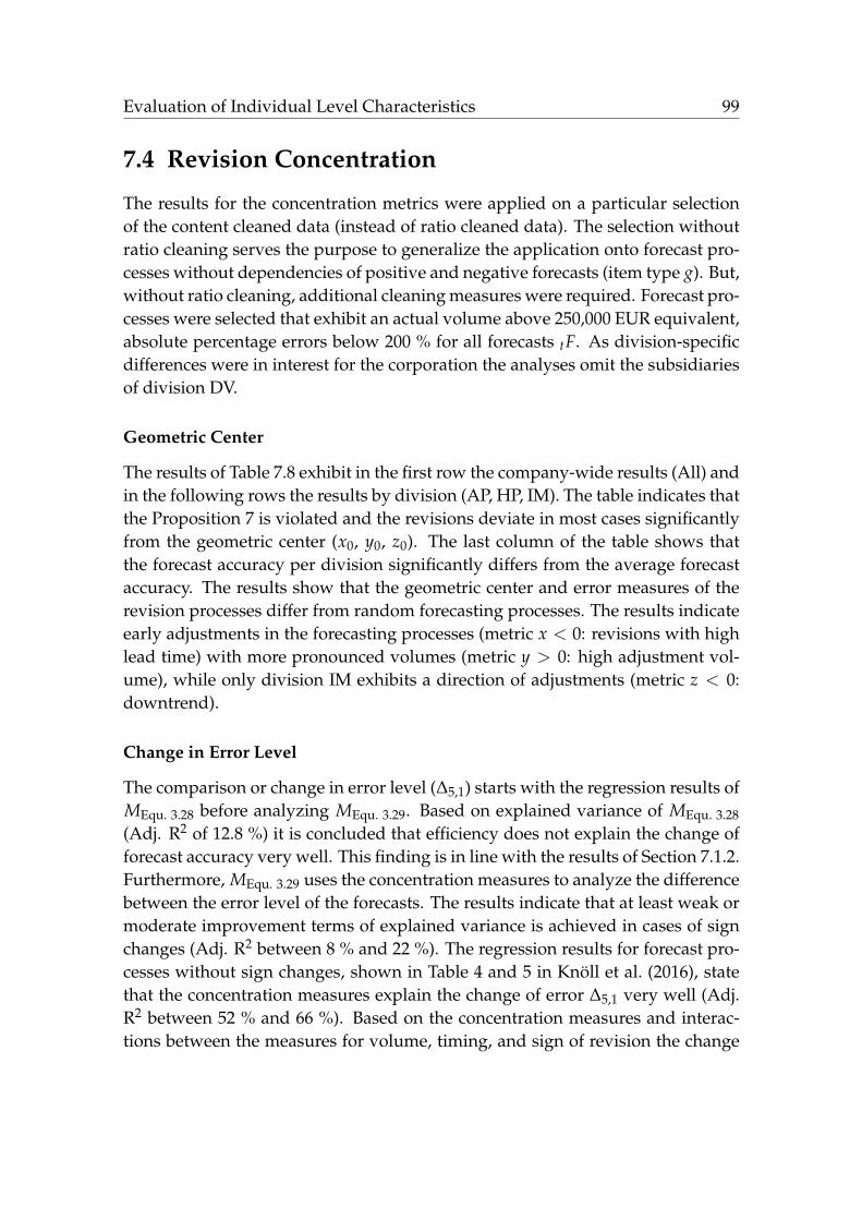
Evaluation of Individual Level Characteristics 99
7.4 Revision Concentration
The results for the concentration metrics were applied on a particular selectionof the content cleaned data (instead of ratio cleaned data). The selection withoutratio cleaning serves the purpose to generalize the application onto forecast pro-cesses without dependencies of positive and negative forecasts (item type g). But,without ratio cleaning, additional cleaning measures were required. Forecast pro-cesses were selected that exhibit an actual volume above 250,000 EUR equivalent,absolute percentage errors below 200 % for all forecasts tF. As division-specificdifferences were in interest for the corporation the analyses omit the subsidiariesof division DV.
Geometric Center
The results of Table 7.8 exhibit in the first row the company-wide results (All) andin the following rows the results by division (AP, HP, IM). The table indicates thatthe Proposition 7 is violated and the revisions deviate in most cases significantlyfrom the geometric center (x0, y0, z0). The last column of the table shows thatthe forecast accuracy per division significantly differs from the average forecastaccuracy. The results show that the geometric center and error measures of therevision processes differ from random forecasting processes. The results indicateearly adjustments in the forecasting processes (metric x < 0: revisions with highlead time) with more pronounced volumes (metric y > 0: high adjustment vol-ume), while only division IM exhibits a direction of adjustments (metric z < 0:downtrend).
Change in Error Level
The comparison or change in error level (∆5,1) starts with the regression results ofMEqu. 3.28 before analyzing MEqu. 3.29. Based on explained variance of MEqu. 3.28
(Adj. R2 of 12.8 %) it is concluded that efficiency does not explain the change offorecast accuracy very well. This finding is in line with the results of Section 7.1.2.Furthermore, MEqu. 3.29 uses the concentration measures to analyze the differencebetween the error level of the forecasts. The results indicate that at least weak ormoderate improvement terms of explained variance is achieved in cases of signchanges (Adj. R2 between 8 % and 22 %). The regression results for forecast pro-cesses without sign changes, shown in Table 4 and 5 in Knöll et al. (2016), statethat the concentration measures explain the change of error ∆5,1 very well (Adj.R2 between 52 % and 66 %). Based on the concentration measures and interac-tions between the measures for volume, timing, and sign of revision the change
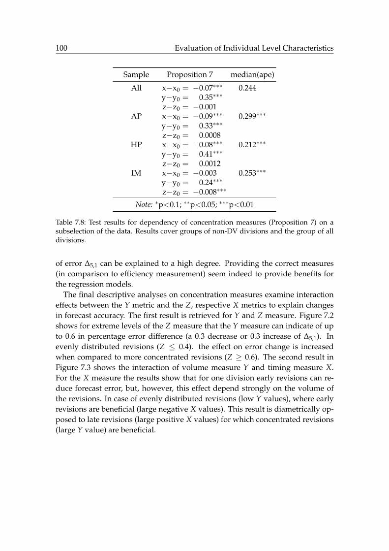
100 Evaluation of Individual Level Characteristics
Sample Proposition 7 median(ape)
All x−x0 = −0.07∗∗∗ 0.244y−y0 = 0.35∗∗∗
z−z0 = −0.001AP x−x0 = −0.09∗∗∗ 0.299∗∗∗
y−y0 = 0.33∗∗∗
z−z0 = 0.0008HP x−x0 = −0.08∗∗∗ 0.212∗∗∗
y−y0 = 0.41∗∗∗
z−z0 = 0.0012IM x−x0 = −0.003 0.253∗∗∗
y−y0 = 0.24∗∗∗
z−z0 = −0.008∗∗∗
Note: ∗p<0.1; ∗∗p<0.05; ∗∗∗p<0.01
Table 7.8: Test results for dependency of concentration measures (Proposition 7) on asubselection of the data. Results cover groups of non-DV divisions and the group of alldivisions.
of error ∆5,1 can be explained to a high degree. Providing the correct measures(in comparison to efficiency measurement) seem indeed to provide benefits forthe regression models.
The final descriptive analyses on concentration measures examine interactioneffects between the Y metric and the Z, respective X metrics to explain changesin forecast accuracy. The first result is retrieved for Y and Z measure. Figure 7.2shows for extreme levels of the Z measure that the Y measure can indicate of upto 0.6 in percentage error difference (a 0.3 decrease or 0.3 increase of ∆5,1). Inevenly distributed revisions (Z ≤ 0.4). the effect on error change is increasedwhen compared to more concentrated revisions (Z ≥ 0.6). The second result inFigure 7.3 shows the interaction of volume measure Y and timing measure X.For the X measure the results show that for one division early revisions can re-duce forecast error, but, however, this effect depend strongly on the volume ofthe revisions. In case of evenly distributed revisions (low Y values), where earlyrevisions are beneficial (large negative X values). This result is diametrically op-posed to late revisions (large positive X values) for which concentrated revisions(large Y value) are beneficial.

Evaluation of Individual Level Characteristics 101
Figure 7.2: Interactions for volume (Y) and direction (Z) measures grouped by item typeand under-/overestimation (no sign change). Figure from the paper (Knöll et al., 2016).
Interim Result
Summarizing the concentration measures leads to an descriptive extension for thetheoretical aspect of the efficiency processes by Nordhaus, explained as follows:the Y concentration metric identifies if the adjustment is made by one or manysteps. The Y metric measures therefore the degree of volume relation between re-visions. As inefficient revisions show systematic behavior they naturally shouldexhibit a low Y measure, as the revisions tend to be more similar to each other.For instance, the value Y = 1 can not be reached for similar revisions – insteadonly with a one time peak where the entire adjustment of a forecasting process ismade at once. Further, the results state that accuracy depends also on the point intime of revisions: the X concentration metric. Early, evenly distributed revisionstend to have reduced error levels – while late, evenly revisions have higher errorlevels. Therefore, based on the interpretation and analyzed data it is arguable: In-efficient, early revisions might have higher accuracy than efficient revisions (withpeak-structure). Overall, the results clearly support Hypothesis 2.
7.5 Summary
This chapter provides the results on individual level analyses of financial fore-casting processes. The empirical analysis of efficiency reveals that forecastingprocesses are not weak form efficient. The inefficiencies of individual level fore-casts are often expected to relate to behaviors of widely established biases, suchas anchoring and adjustment. Analyses that account for these biases did indicate
102 Evaluation of Individual Level Characteristics
Figure 7.3: Interaction effect for timing (X) and volume (Y) measures of division HP (over-estimation). Figure from the paper (Knöll et al., 2016).
that individual level biases are at play. But, detailed inspection of the analysessuggest that other underlying influences might form these behavioral aspects.
Efficiency and Efficiency Hypothesis
The analyses reveal that weak form forecast efficiency can not be stated and thereduction of lead time is not solely associated with accuracy increase, especiallyfor December forecasts. Furthermore, the analyses reveal that weak forecast effi-ciency is not invariably connected to accurate forecasting – and as a consequencethereof the validity of the forecast efficiency hypothesis for the analyzed corpo-rate internal forecasts must be rejected. However, with regard to market effi-ciency, it would be interesting to analyze data from the financial markets to de-termine whether similar effects exist there.
Behavioral Individual Level Reasoning
The analyses of A&A metrics and concentration metrics revealed interesting in-sights in individual level behavior of forecasting processes. First, the results in-dicate that the influence of the A&A effect intensifies for previous year’s actualsin November and December. Second, depending on the kind of metric used forA&A biases, performance for identification is different, and metrics do correlatewith error metrics in differing ways. Utilizing advanced approaches for patternidentification of A&A can improve predictive performance due to error correla-tion. Third, complex descriptive measurement of whole forecast processes withBandwidth Models and concentration measures show that important informa-

Evaluation of Individual Level Characteristics 103
tion is inherent in forecast processes in their entirety. Analyses that base solely onthe examination of single forecasts misses opportunities for understanding andcorrection, as revisions provide meaningful information based on the dimensionstime, volume, and direction of adjustments.
Indication of Further Influences
However, the findings show that anchoring is most pronounced in the last twomonths of a year, and the strength of bias-related patterns increase as lead timedecreases, in particular for actuals approaching the end of a fiscal year. Theseresults provide further indications that other influences than individual bias areat play and suggesting reasons why Proposition (P4) does not hold. The rejectionof the efficiency hypothesis for the analyzed internal corporate forecasts is animportant contradiction to the common expectations in forecasting research. Thedistorting influence that seem to impact forecasting especially at the end of theyear, provides the argumentation for the next chapter.

Chapter 8
Evaluation of Aggregate LevelBusiness Characteristics
This chapter presents the empirical results of the aggregate level analysis.These consist of the ratio metric analysis, which supports the existence of
targets at an aggregate level, the explanation framework for beneficial inefficien-cies and the examination of organizational relations. The examination analyzesin particular the target, revision and organizational dependencies. The chapterconcludes by a summarizing interpretation of the results.
8.1 Ratio Metric: Validity
The results for the validity analysis on lag-shifted unnormalized ratio calculationis shown in Table 8.1. The standard deviation of ratios only decreases for thefiscal year from January to December (column l = 0, from 3.40 to 2.08). Whena different starting point than January is chosen, the aggregation results for allother alternatives in increased standard deviation of ratios instead. For instance,when starting in April as the first month of the aggregation (column l = 3), thestandard deviation of ratio starts with 4.80, decreases for invoices that aggregateApril and May to 3.63, but end up with 8.21 for the last aggregation that coversall calculated ratios based on the starting month April.
105
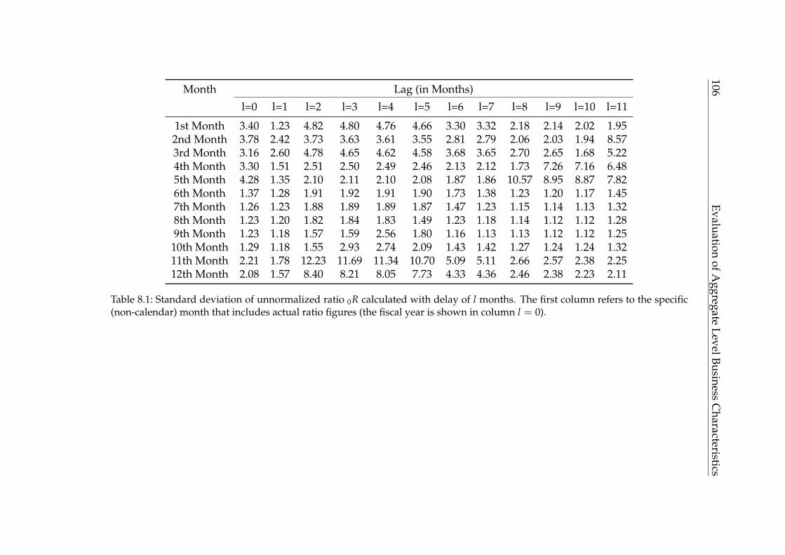
106Evaluation
ofAggregate
LevelBusinessC
haracteristics
Month Lag (in Months)
l=0 l=1 l=2 l=3 l=4 l=5 l=6 l=7 l=8 l=9 l=10 l=11
1st Month 3.40 1.23 4.82 4.80 4.76 4.66 3.30 3.32 2.18 2.14 2.02 1.952nd Month 3.78 2.42 3.73 3.63 3.61 3.55 2.81 2.79 2.06 2.03 1.94 8.573rd Month 3.16 2.60 4.78 4.65 4.62 4.58 3.68 3.65 2.70 2.65 1.68 5.224th Month 3.30 1.51 2.51 2.50 2.49 2.46 2.13 2.12 1.73 7.26 7.16 6.485th Month 4.28 1.35 2.10 2.11 2.10 2.08 1.87 1.86 10.57 8.95 8.87 7.826th Month 1.37 1.28 1.91 1.92 1.91 1.90 1.73 1.38 1.23 1.20 1.17 1.457th Month 1.26 1.23 1.88 1.89 1.89 1.87 1.47 1.23 1.15 1.14 1.13 1.328th Month 1.23 1.20 1.82 1.84 1.83 1.49 1.23 1.18 1.14 1.12 1.12 1.289th Month 1.23 1.18 1.57 1.59 2.56 1.80 1.16 1.13 1.13 1.12 1.12 1.25
10th Month 1.29 1.18 1.55 2.93 2.74 2.09 1.43 1.42 1.27 1.24 1.24 1.3211th Month 2.21 1.78 12.23 11.69 11.34 10.70 5.09 5.11 2.66 2.57 2.38 2.2512th Month 2.08 1.57 8.40 8.21 8.05 7.73 4.33 4.36 2.46 2.38 2.23 2.11
Table 8.1: Standard deviation of unnormalized ratio 0R calculated with delay of l months. The first column refers to the specific(non-calendar) month that includes actual ratio figures (the fiscal year is shown in column l = 0).

Evaluation of Aggregate Level Business Characteristics 107
The result suggests that a proxy for a end of year target only exists in the fiscalyear, supporting Hypothesis 3. The further expectation that other sub-annual in-fluences exist could explain the differences in the lagged aggregates of the othermonths. Also, the aggregation and lag aspect depends on the business cycle,which in the sample corporation is the calendar year. The closure of yearly ac-counts may vary for other corporations and in those cases the correct setting ofthe lag is assumed to be different. According to Section 4.1, all further analyseswill base on ratios calculated with zero lag.
8.2 Ratio Metric: Earnings Target Existence
Decrease of Standard Deviation
The results for the validity of a earnings target existence on division level isshown in Table 8.2. Here, standard deviation is calculated over the aggregatedratios of entities belonging to a division. The table shows decreasing standard de-viation of the ratio over time for division AP. For the other divisions its behavioris more like a martingale process, finalizing with minimum standard deviationin December. For instance, the standard deviation in January for the businessdivision AP is 1.20, which decreases to 0.55 in December. Another example ofdecreased standard deviation is shown for the business division HP that reducesby 28 % (from 1.06 to 0.76). For all divisions except DV, the accumulated ratiosapproach their minimum values in December, when approaching the end of afiscal year. However, division DV has decreased standard deviation at the end ofthe fiscal year when compared to January. The result clearly indicates a divisionspecific converging actual ratio while approaching the end of year.
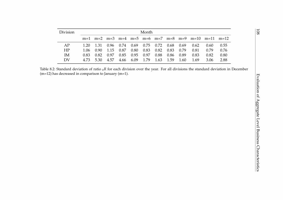
108Evaluation
ofAggregate
LevelBusinessC
haracteristics
Division Month
m=1 m=2 m=3 m=4 m=5 m=6 m=7 m=8 m=9 m=10 m=11 m=12
AP 1.20 1.31 0.96 0.74 0.69 0.75 0.72 0.68 0.69 0.62 0.60 0.55HP 1.06 0.90 1.15 0.87 0.80 0.83 0.82 0.83 0.79 0.81 0.79 0.76IM 0.83 0.82 0.97 0.85 0.95 0.97 0.88 0.86 0.89 0.83 0.82 0.80DV 4.73 5.30 4.57 4.66 6.09 1.79 1.63 1.59 1.60 1.69 3.06 2.88
Table 8.2: Standard deviation of ratio 0R for each division over the year. For all divisions the standard deviation in December(m=12) has decreased in comparison to January (m=1).
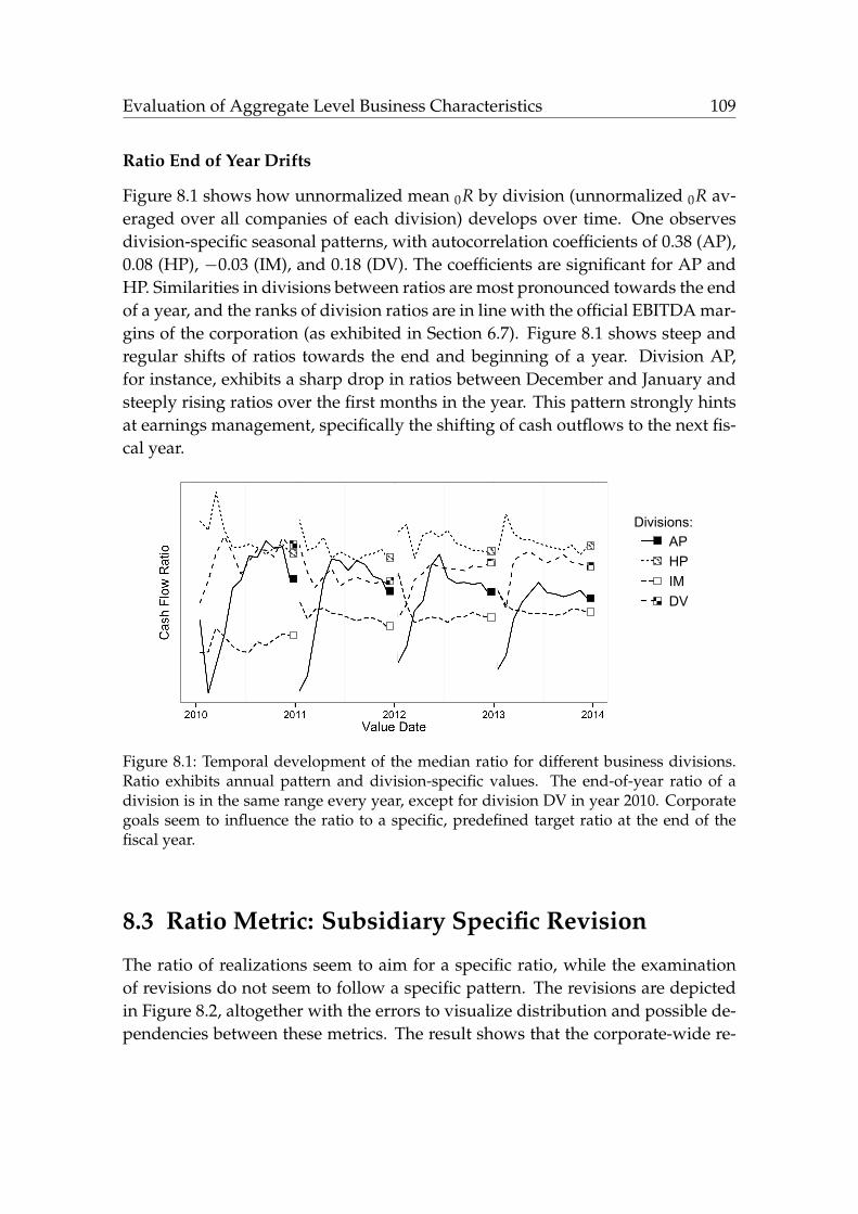
Evaluation of Aggregate Level Business Characteristics 109
Ratio End of Year Drifts
Figure 8.1 shows how unnormalized mean 0R by division (unnormalized 0R av-eraged over all companies of each division) develops over time. One observesdivision-specific seasonal patterns, with autocorrelation coefficients of 0.38 (AP),0.08 (HP), −0.03 (IM), and 0.18 (DV). The coefficients are significant for AP andHP. Similarities in divisions between ratios are most pronounced towards the endof a year, and the ranks of division ratios are in line with the official EBITDA mar-gins of the corporation (as exhibited in Section 6.7). Figure 8.1 shows steep andregular shifts of ratios towards the end and beginning of a year. Division AP,for instance, exhibits a sharp drop in ratios between December and January andsteeply rising ratios over the first months in the year. This pattern strongly hintsat earnings management, specifically the shifting of cash outflows to the next fis-cal year.
Divisions: ! AP ! HP ! IM ! DV
Figure 8.1: Temporal development of the median ratio for different business divisions.Ratio exhibits annual pattern and division-specific values. The end-of-year ratio of adivision is in the same range every year, except for division DV in year 2010. Corporategoals seem to influence the ratio to a specific, predefined target ratio at the end of thefiscal year.
8.3 Ratio Metric: Subsidiary Specific Revision
The ratio of realizations seem to aim for a specific ratio, while the examinationof revisions do not seem to follow a specific pattern. The revisions are depictedin Figure 8.2, altogether with the errors to visualize distribution and possible de-pendencies between these metrics. The result shows that the corporate-wide re-

110 Evaluation of Aggregate Level Business Characteristics
visions hardly indicate a specific pattern. To analyze whether a pattern for therevisions exists within the entity, the revisions (and errors) are normalized basedon the history of ratios. The importance of this entity specific normalization is de-picted with Figures 8.2 and 8.3. Without normalization the ratio of the forecastsdistributes with an center of zero error and zero revision. Instead, with normal-ization the relation between error and revision shows a clear negative pattern.One could argue that without normalization the forecasts seem to be “efficient”and without predictive value, while they obviously show some dependency thatsuggests “inefficiency” for normalized ratio revisions. For analytic and predic-tive purposes the entity-specific normalization is obviously beneficial, allowingto relate the errors and revisions.
Error (not normalized
) 1E
Revision (not normalized) 12R
Figure 8.2: Relation between not normalized revisions and not normalized error of enti-ties. Revisions and errors scatter, following a Gaussian normal-distribution with a centerof zero revision.
8.4 Efficiency at Aggregate Level
Previous sections offers a perspective that entity specific behavior might influ-ence the forecasting process. This motivates the following analyses for efficiencyat the aggregate level, as it is assumed that forecasting processes has to differ inefficiency for the single item forecasting and the entity level forecasting. Further-more, it is expected that influences are more pronounced at the entity level.
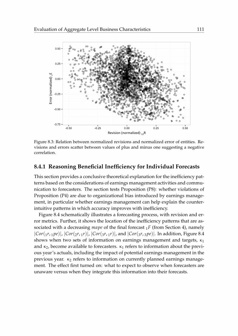
Evaluation of Aggregate Level Business Characteristics 111
Error (normalized
) 1E
Revision (normalized) 12R
Figure 8.3: Relation between normalized revisions and normalized error of entities. Re-visions and errors scatter between values of plus and minus one suggesting a negativecorrelation.
8.4.1 Reasoning Beneficial Inefficiency for Individual Forecasts
This section provides a conclusive theoretical explanation for the inefficiency pat-terns based on the considerations of earnings management activities and commu-nication to forecasters. The section tests Proposition (P8): whether violations ofProposition (P4) are due to organizational bias introduced by earnings manage-ment, in particular whether earnings management can help explain the counter-intuitive patterns in which accuracy improves with inefficiency.
Figure 8.4 schematically illustrates a forecasting process, with revision and er-ror metrics. Further, it shows the location of the inefficiency patterns that are as-sociated with a decreasing mape of the final forecast 1F (from Section 4), namely|Cor(1r, 1pe)|, |Cor(2r, 1r)|, |Cor(3r, 1r)|, and |Cor(3r, 3pe)|. In addition, Figure 8.4shows when two sets of information on earnings management and targets, κ1
and κ2, become available to forecasters. κ1 refers to information about the previ-ous year’s actuals, including the impact of potential earnings management in theprevious year. κ2 refers to information on currently planned earnings manage-ment. The effect first turned on: what to expect to observe when forecasters areunaware versus when they integrate this information into their forecasts.
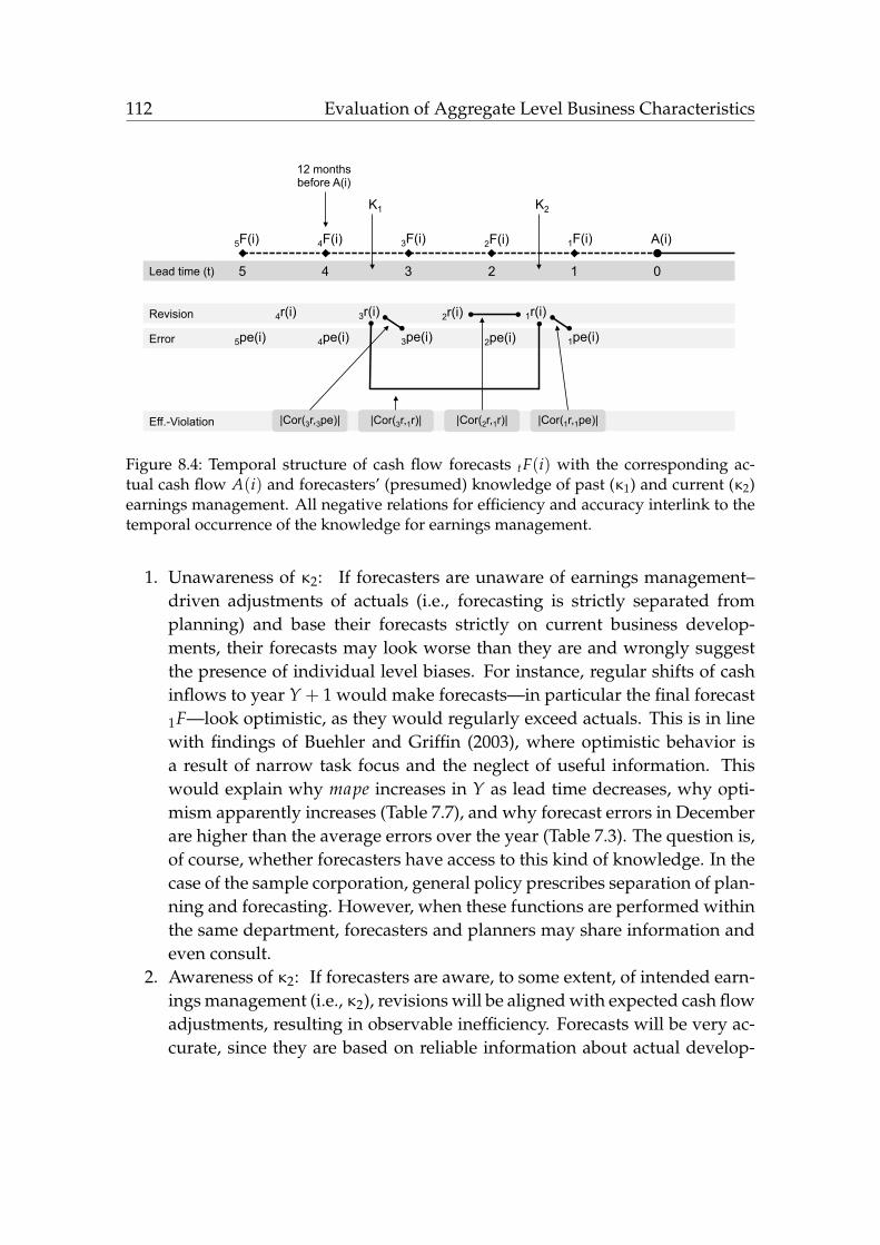
112 Evaluation of Aggregate Level Business Characteristics
Eff.-Violation
Error
Revision 4r(i) 3r(i) 1r(i) 2r(i)
5F(i) 4F(i) 3F(i) 1F(i) 2F(i) A(i)
Lead time (t) 5 4 3 2 1 0
Κ2
12 months before A(i)
Κ1
5pe(i) 4pe(i) 3pe(i) 1pe(i) 2pe(i)
|Cor(1r,1pe)| |Cor(2r,1r)| |Cor(3r,3pe)| |Cor(3r,1r)|
Figure 8.4: Temporal structure of cash flow forecasts tF(i) with the corresponding ac-tual cash flow A(i) and forecasters’ (presumed) knowledge of past (κ1) and current (κ2)earnings management. All negative relations for efficiency and accuracy interlink to thetemporal occurrence of the knowledge for earnings management.
1. Unawareness of κ2: If forecasters are unaware of earnings management–driven adjustments of actuals (i.e., forecasting is strictly separated fromplanning) and base their forecasts strictly on current business develop-ments, their forecasts may look worse than they are and wrongly suggestthe presence of individual level biases. For instance, regular shifts of cashinflows to year Y + 1 would make forecasts—in particular the final forecast1F—look optimistic, as they would regularly exceed actuals. This is in linewith findings of Buehler and Griffin (2003), where optimistic behavior isa result of narrow task focus and the neglect of useful information. Thiswould explain why mape increases in Y as lead time decreases, why opti-mism apparently increases (Table 7.7), and why forecast errors in Decemberare higher than the average errors over the year (Table 7.3). The question is,of course, whether forecasters have access to this kind of knowledge. In thecase of the sample corporation, general policy prescribes separation of plan-ning and forecasting. However, when these functions are performed withinthe same department, forecasters and planners may share information andeven consult.
2. Awareness of κ2: If forecasters are aware, to some extent, of intended earn-ings management (i.e., κ2), revisions will be aligned with expected cash flowadjustments, resulting in observable inefficiency. Forecasts will be very ac-curate, since they are based on reliable information about actual develop-
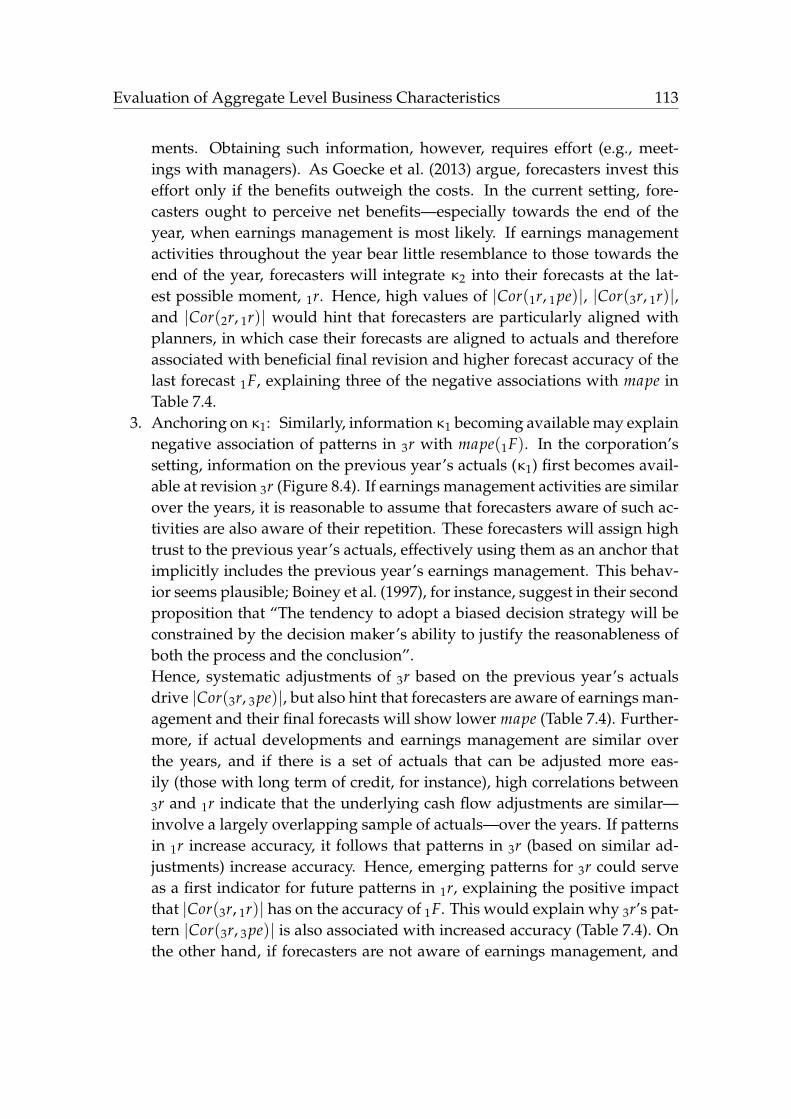
Evaluation of Aggregate Level Business Characteristics 113
ments. Obtaining such information, however, requires effort (e.g., meet-ings with managers). As Goecke et al. (2013) argue, forecasters invest thiseffort only if the benefits outweigh the costs. In the current setting, fore-casters ought to perceive net benefits—especially towards the end of theyear, when earnings management is most likely. If earnings managementactivities throughout the year bear little resemblance to those towards theend of the year, forecasters will integrate κ2 into their forecasts at the lat-est possible moment, 1r. Hence, high values of |Cor(1r, 1pe)|, |Cor(3r, 1r)|,and |Cor(2r, 1r)| would hint that forecasters are particularly aligned withplanners, in which case their forecasts are aligned to actuals and thereforeassociated with beneficial final revision and higher forecast accuracy of thelast forecast 1F, explaining three of the negative associations with mape inTable 7.4.
3. Anchoring on κ1: Similarly, information κ1 becoming available may explainnegative association of patterns in 3r with mape(1F). In the corporation’ssetting, information on the previous year’s actuals (κ1) first becomes avail-able at revision 3r (Figure 8.4). If earnings management activities are similarover the years, it is reasonable to assume that forecasters aware of such ac-tivities are also aware of their repetition. These forecasters will assign hightrust to the previous year’s actuals, effectively using them as an anchor thatimplicitly includes the previous year’s earnings management. This behav-ior seems plausible; Boiney et al. (1997), for instance, suggest in their secondproposition that “The tendency to adopt a biased decision strategy will beconstrained by the decision maker’s ability to justify the reasonableness ofboth the process and the conclusion”.Hence, systematic adjustments of 3r based on the previous year’s actualsdrive |Cor(3r, 3pe)|, but also hint that forecasters are aware of earnings man-agement and their final forecasts will show lower mape (Table 7.4). Further-more, if actual developments and earnings management are similar overthe years, and if there is a set of actuals that can be adjusted more eas-ily (those with long term of credit, for instance), high correlations between3r and 1r indicate that the underlying cash flow adjustments are similar—involve a largely overlapping sample of actuals—over the years. If patternsin 1r increase accuracy, it follows that patterns in 3r (based on similar ad-justments) increase accuracy. Hence, emerging patterns for 3r could serveas a first indicator for future patterns in 1r, explaining the positive impactthat |Cor(3r, 1r)| has on the accuracy of 1F. This would explain why 3r’s pat-tern |Cor(3r, 3pe)| is also associated with increased accuracy (Table 7.4). Onthe other hand, if forecasters are not aware of earnings management, and

114 Evaluation of Aggregate Level Business Characteristics
give high weight to their own business expectations rather than the previ-ous year’s actuals, no patterns will be observable either in 3r or in 1r. Thiswould explain why there is generally an increase in mape at 3r observable,while there is no such increase if 3r does exhibit inefficiency patterns.
Interim Result
The explanation framework hypothesizes when to expect structure in forecastingprocesses to be negative and due to cognitive bias – and where to expect a positiveassociation between accuracy and structure that hints to organizational-level is-sues masking cognitive biases at the individual forecaster level. In sum, earningsmanagement appears to provide a conclusive explanation for the results regard-ing individual level biases, mape increasing with decreasing lead time, and thefour counter-intuitive patterns associated with improvements in the accuracy ofthe final forecast (Table 7.4). If inefficiencies are found that are associated with in-creased accuracy, it’s recommend to consider organizational-level issues to driveforecasting and rethink organizational structure before wrong conclusions aredrawn with respect to the quality of forecasters (individual level).
8.4.2 Testing Aggregate Level Efficiency
As noted before, the forecast efficiency is an important goal of forecasting pro-cesses. The baseline of forecast efficiency for M∅ on ratio basis is shown inTable 8.3. The result indicates very high inefficiency for revisions and the de-scending error of the forecast resulting from that revision made by experts. Forinstance, revision 23R and subsequent error 2E exhibit a correlation coefficient of−0.27. Further, the autocorrelation of revisions at shift one exhibits high negativecorrelation, while there is indeed a high negative correlation between 45R and12R. This supports the argument of revisions aligned to seasonal pattern, whileit is noted that this differs from the argument of end of year values – since theseefficiency characteristics does not only start in the last quarter of the year, insteadthe analyzed forecast processes cover the whole year.
8.5 Organizational Relations
This section covers analyses of organizational influences with dependencies oftarget ratio and revision ratio. In addition, the section covers ratio analyses oninflicting goals that highlight important implications for the forecasting processwithin the corporation.

Evaluation of Aggregate Level Business Characteristics 115
4E 3E 2E 1E 34R 23R 12R
45R −0.24∗∗∗ −0.11∗∗∗ −0.08∗∗∗ 0.02 −0.22∗∗∗ −0.05∗∗∗ −0.13∗∗∗
34R −0.19∗∗∗ −0.02 0.01 −0.23∗∗∗ −0.03∗
23R −0.27∗∗∗ −0.10∗∗∗ −0.24∗∗∗
12R −0.31∗∗∗
Note: ∗p<0.1; ∗∗p<0.05; ∗∗∗p<0.01; Observations: 2,355.
Table 8.3: Spearman correlation and significance levels on ratio level of revisions and er-rors. Results show correlation values and significance levels of experts, without any cor-rection (baseline model M∅). Consecutive revisions and errors (in the diagonals) exhibitvery high correlations.
8.5.1 Error Dependencies on Earnings Target
The resulting regression models MBasic (Definition 7) and MOrga (Defintion 8) areshown in Table 8.4. The integration of TargetDiff shows clearly strong influenceon the response variable (ratio error), while the estimates’ magnitude of the otherdependent variables are reduced. Analysis of the R2-values of the models sup-ports Hypothesis 4 (R2-value of 0.310 for Model MBasic compared to 0.608 forModel MOrga).
Dep. Variables Estimates Model MBasic Estimates Model MOrga
Constant 0.178∗∗∗ −0.027∗∗∗
1R −0.541∗∗∗ −0.000312R −0.125∗∗∗ −0.039∗∗
TargetDiff (Not Utilized) 0.735∗∗∗
R2 0.310∗∗∗ 0.608∗∗∗
Note: ∗p<0.1; ∗∗p<0.05; ∗∗∗p<0.01; Observations: 2,355.
Table 8.4: Analyses for the influence of target difference by comparison of regressionmodels. The error 1E is regressed with two models MBasic and MOrga. Estimate of Tar-getDiff strongly influences the error in ratio. The explanatory power (R2-value) nearlydoubles by incorporating TargetDiff information.
Detailed results for the regression model of MOrga is shown in Table 8.5. Dif-ference from target has by far the strongest association with ratio error 1E, whichbasically means that at the ratio level, the presumed margin target is the best in-dicator of how to adjust forecasts in order to increase accuracy. Last forecast ratio1R has no significant effect on 1E. Last revision 12R has a small but significant neg-ative association with 1E. Hence, in line with Amir and Ganzach (1998) observed

116 Evaluation of Aggregate Level Business Characteristics
Variable Estimate 90 % CI
Constant −0.027∗∗∗ (−0.042, −0.012)1R −0.0003 (−0.033, 0.033)12R −0.039∗∗ (−0.071, −0.007)DiffTarg 0.735∗∗∗ (0.706, 0.763)
Observations 2,355R2 0.608Residual Std. Error 0.202 (df = 2351)F Statistic 1,216.089∗∗∗ (df = 3; 2351)
Note: ∗p<0.1; ∗∗p<0.05; ∗∗∗p<0.01; CI = confidence interval.
Table 8.5: Analytical model for the difference between expert forecast and actual ratio(1E) for the entire year. The model utilizes normalized ratio of the last forecast, relativerevision and the ratio difference from the entity specific target ratio. Difference fromtarget has the strongest effect. Actuals and forecast ratios are derived from aggregatedcash flow data.
estimates show that the forecasters tend to be pessimistic and underreact withtheir revisions (Constant negative, 12R negative).
Table 8.6 shows the results for the same regression performed on the subset ofDecember actuals. Compared to the year model, difference from target in Decemberhas a greater effect on ratio error. This is in line with the previous suggestionthat if earnings management is present, effects will be most pronounced towardsthe end of the year. The explaining conclusion of this finding can be stated asan enhancement of Ball and Watts (1972). Earnings targets of entities drive thesub-martingale process behavior via accounting practices (smoothed cash flowactuals), stating that the expectation of income is a function of time. To find aspecific form of time series behavior seems difficult, because incomes seem todepend from an organizational bias that probably varies over time. But yearlyearnings targets show one potential and likely explanation.
This interpretation is also supported by the fact that the proportion of ex-plained variance for the December model (Adj. R2 = 0.729) is higher than for theyear model (Adj. R2 = 0.608) and that the regression constant, the corporation-wide baseline for the normalized ratio, indicates lower error in December. Thedrift towards earnings targets turns out to be a valuable predictor for cash flowforecast accuracy at the aggregate level of annual return.
Table 8.7 shows the results for the same regression performed on the subset ofJanuary actuals. The estimate of the Constant and 1R has a significant influence,while 12R and DiffTarg are above the 0.05 significance level. Compared to the

Evaluation of Aggregate Level Business Characteristics 117
Variable Estimate 90 % CI
Constant −0.051∗∗ (−0.090, −0.013)1R 0.052 (−0.030, 0.133)12R −0.060 (−0.150, 0.030)DiffTarg 0.850∗∗∗ (0.773, 0.927)
Observations 217R2 0.729Residual Std. Error 0.158 (df = 213)F Statistic 190.621∗∗∗ (df = 3; 213)
Note: ∗p<0.1; ∗∗p<0.05; ∗∗∗p<0.01; CI = confidence interval.
Table 8.6: Analytical model for the difference between expert forecast and actual ratio (1E)for months of December. The model utilizes normalized ratio of the last forecast, relativerevision and the ratio difference from the entity specific target ratio. Difference fromtarget has the strongest effect. Actuals and forecast ratios are derived from aggregatedcash flow data.
December model, difference from target in December has a far smaller effect onratio error, which is in line with the suggestion that earnings management will bemost pronounced towards the end of year. While earnings management at theend of year leads to adjustments that entail shifts of cash flows in January, thefinding underlines that forecast errors in January seem less systematic. In fact,the linear regression model of January can not account for the shifts that wererequired to reach the target in the previous year1.
This interpretation is also supported by the fact that the proportion of ex-plained variance for the January model (Adj. R2 = 0.324) is lower than for the De-cember model (Adj. R2 = 0.729) and that the regression constant, the corporation-wide baseline for the normalized ratio, indicates higher error in January.
In summary, the results support Proposition (P8), that organizational biasesrelated to targets of earnings margin and earnings management are present andlead (to a large extent) to the ambiguities regarding Proposition (P4). The resultsshow that organizational biases help explain counter-intuitive findings on theindividual level, and that individual level analysis will lead to wrong conclusionsif organizational-level biases are not accounted for.
1One can assume that such information strongly improve the model performance in January.

118 Evaluation of Aggregate Level Business Characteristics
Variable Estimate 90 % CI
Constant 0.213∗∗∗ (0.124, 0.301)1R −0.548∗∗∗ (−0.751, −0.345)12R −0.058 (−0.195, 0.079)DiffTarg 0.156∗ (0.004, 0.309)
Observations 204R2 0.388Residual Std. Error 0.324 (df = 200)F Statistic 42.210∗∗∗ (df = 3; 200)
Note: ∗p<0.1; ∗∗p<0.05; ∗∗∗p<0.01; CI = confidence interval.
Table 8.7: Analytical model for the difference between expert forecast and actual ratio (1E)for months of January. The model utilizes normalized ratio of the last forecast, relativerevision and the ratio difference from the entity specific target ratio. Current ratio forecasthas the strongest effect. Actuals and forecast ratios are derived from aggregated cash flowdata.
8.5.2 Dependencies on Revision
This section considers means of forecast improvement due to regular patterns inforecast revisioning. The focus is analyzing how business forecasts are adjustedto exploit possible improvements for the accuracy of forecasts with lower leadtime. The assumption is that direction and magnitude of the final revision inaggregated forecasts can be related to suggested earnings targets, providing themeans of improving the accuracy of longer-term cash flow forecasts.
Revision: Direction and Strength Influenced by Targets
Regression outcomes for revision magnitude (Model MDef. 9) are shown in Ta-ble 8.8. The outcome shows that an expert’s revisioning can indeed be partlyexplained by TargetDiff and Month. Changes in forecast ratios through a revi-sioning of cash flows increases with TargetDiff – high distance of a forecast ratioto the presumed target ratio is associated with high the adjustments of the ratiothrough revisioning, and declines when approaching the end of a fiscal year. Thesignificance of both estimates is surprising, as this means that the magnitude ofthe final revisions of cash flows, at the aggregated ratio level, is predictable tosome extent.
Table 8.9 shows the result of the regression of revision with significance levels(MDef. 10). The results indicate that revision at the ratio level is significantly pos-itively related to the magnitude of difference from target, indicating that forecast

Evaluation of Aggregate Level Business Characteristics 119
Dep. Variables for |12R| Estimates
Constant 0.184 ∗∗∗
| TargetDiff | 0.085 ∗∗∗
Month −0.005 ∗∗∗
Observations: 2,355Significance levels: ∗p<0.1; ∗∗p<0.05; ∗∗∗p<0.01
Table 8.8: Analytical model regressing the magnitude in forecast ratio through absolutedifference from target and month. The higher the distance of the forecast ratio to thetarget ratio, the higher the adjustments of the ratio revisioning. Absolute change declineswhen approaching the end of a fiscal year.
ratios increase through the final revisioning cycle. The higher the absolute dis-tance from T(0R), the more the cash flow forecasts (1R) are adjusted to increasethe ratio. In addition, over the months in a year the last revision (12R) decreasesthe revision and therefore the forecast ratio (1R). These results hint at experts ad-justing their cash flows in a way to reach a position above T(0R). Forecast ratiosare revised upwards, with adjustments getting smaller when approaching T(0R).Considering the negative estimate of Month, this leads to approaching T(0R) to-wards the end of a year.
Dep. Variables for 12R Estimates
Constant 0.025 ∗
| TargetDiff | 0.054 ∗∗
Month −0.004 ∗∗∗
Observations: 2,355Significance levels: ∗p<0.1; ∗∗p<0.05; ∗∗∗p<0.01
Table 8.9: Analytical model regressing the forecast revision through absolute differencefrom target and month. The adjustments of the ratio revisioning is positively related tothe distance of the forecast ratio to the target ratio, indicating that forecast ratios increasethrough the final revision. Revision declines when approaching the end of a fiscal year.
Regression results for revision based on TargetDiff (MDef. 11) are shown in Ta-ble 8.10. The significance of the negative estimate indicates that 1R decrease whenT(0R) is already met and increased when 1R is below T(0R).
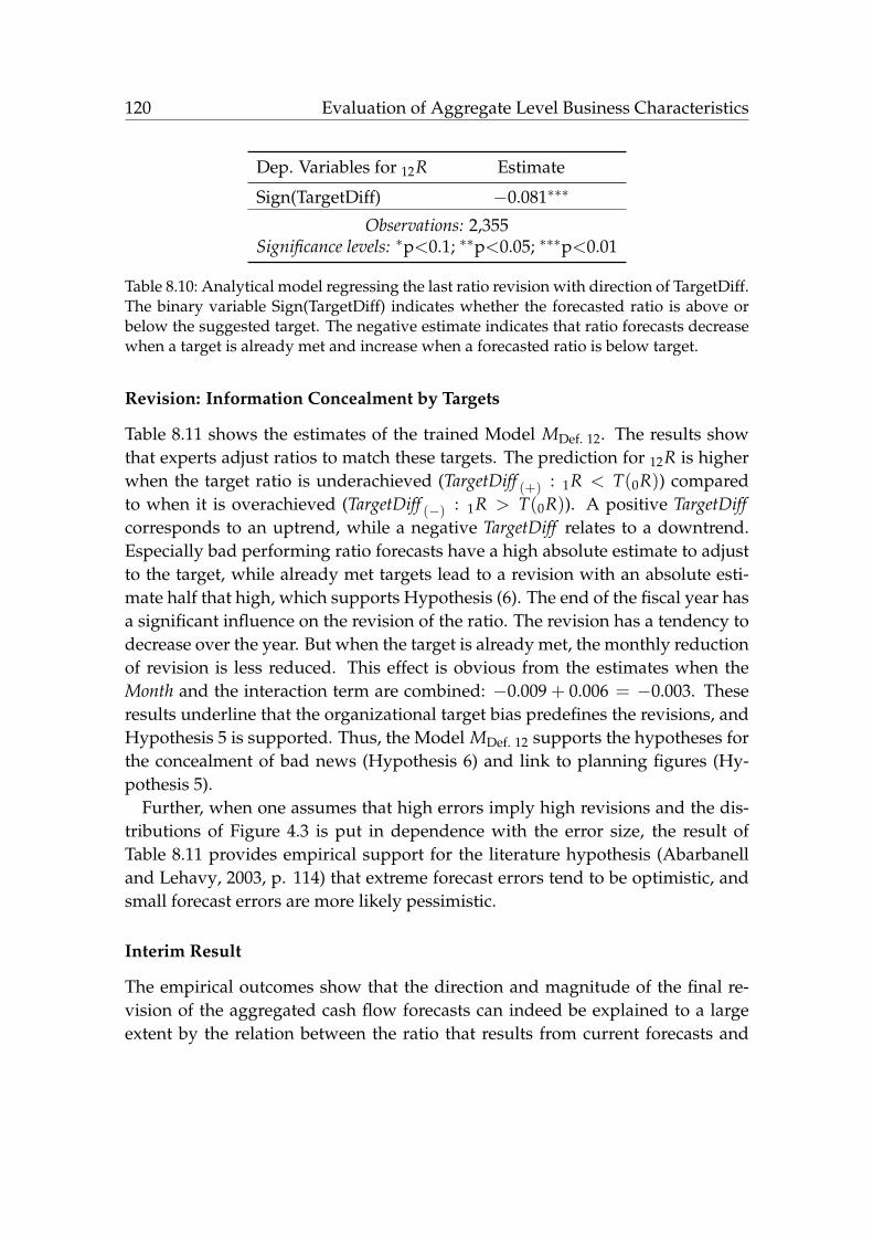
120 Evaluation of Aggregate Level Business Characteristics
Dep. Variables for 12R Estimate
Sign(TargetDiff) −0.081∗∗∗
Observations: 2,355Significance levels: ∗p<0.1; ∗∗p<0.05; ∗∗∗p<0.01
Table 8.10: Analytical model regressing the last ratio revision with direction of TargetDiff.The binary variable Sign(TargetDiff) indicates whether the forecasted ratio is above orbelow the suggested target. The negative estimate indicates that ratio forecasts decreasewhen a target is already met and increase when a forecasted ratio is below target.
Revision: Information Concealment by Targets
Table 8.11 shows the estimates of the trained Model MDef. 12. The results showthat experts adjust ratios to match these targets. The prediction for 12R is higherwhen the target ratio is underachieved (TargetDiff (+) : 1R < T(0R)) comparedto when it is overachieved (TargetDiff (−) : 1R > T(0R)). A positive TargetDiffcorresponds to an uptrend, while a negative TargetDiff relates to a downtrend.Especially bad performing ratio forecasts have a high absolute estimate to adjustto the target, while already met targets lead to a revision with an absolute esti-mate half that high, which supports Hypothesis (6). The end of the fiscal year hasa significant influence on the revision of the ratio. The revision has a tendency todecrease over the year. But when the target is already met, the monthly reductionof revision is less reduced. This effect is obvious from the estimates when theMonth and the interaction term are combined: −0.009 + 0.006 = −0.003. Theseresults underline that the organizational target bias predefines the revisions, andHypothesis 5 is supported. Thus, the Model MDef. 12 supports the hypotheses forthe concealment of bad news (Hypothesis 6) and link to planning figures (Hy-pothesis 5).
Further, when one assumes that high errors imply high revisions and the dis-tributions of Figure 4.3 is put in dependence with the error size, the result ofTable 8.11 provides empirical support for the literature hypothesis (Abarbanelland Lehavy, 2003, p. 114) that extreme forecast errors tend to be optimistic, andsmall forecast errors are more likely pessimistic.
Interim Result
The empirical outcomes show that the direction and magnitude of the final re-vision of the aggregated cash flow forecasts can indeed be explained to a largeextent by the relation between the ratio that results from current forecasts and
Evaluation of Aggregate Level Business Characteristics 121
Dep. Variables for 12R Estimates
TargetDiff(+) 0.145 ∗∗∗
TargetDiff(−) −0.063 ∗∗∗
Month −0.009 ∗∗∗
TargetDiff(+)×Month 0.006 ∗∗
Observations: 2,355Significance levels: ∗p<0.1; ∗∗p<0.05; ∗∗∗p<0.01
Table 8.11: Analytical model regressing revision with dependencies of TargetDiff andMonth. Model MDef. 12 explains dependencies of revision on the difference from the tar-get. The result shows that revision in ratio is higher, if the forecast is below the target(TargetDiff(+)) when compared to forecasts above the target (TargetDiff(−)).
the presumed accountants’ earnings targets.Overall, these results show that forecasting processes do not describe random
walks and provide strong indication that cash flow ratios are adjusted to con-verge to predefined target ratios. The difference of the forecast from this targetturns out to be a strong predictor for subsequent revision direction and volume.This allows for anticipating the final revision and therefore the upcoming expertforecasts to some extent. Knowledge of how forecasts will be adjusted later on byexperts allows improving longer–term forecast ratios, considering that forecastaccuracy overall increases with decreasing lead time. For instance, a model forthe last revision 12R can partially anticipate at time t = 2 the final forecast 1R inadvance.
8.5.3 Impact on Organizational Goals
Model MDef. 13 in Table 8.12 shows that Constant is not significant, while 1E hasa significant effect on 12R, which supports Hypothesis (7). Revisioning in ModelMDef. 14 is organizationally biased by 1E and experts adjust the ratio in relationto TargetDiff . As anticipated, the organizational bias TargetDiff distorts the fore-casting process according to the result for the Hypotheses (5) and (6). Expectingthat accurate forecasting is the primary goal of forecasting processes, the strengthof the estimate of 1E is expected to be the highest. However, estimates clearlyshow that TargetDiff overlays this goal with an estimate more than five times thathigh. These estimates suggests that the model assign more importance to the tar-get (T(0R)) than to the actual ratio (0R) for the forecaster’s revisioning (12R). Thegoal of managers seems to be different from the corporation’s original goal of theforecasting process, which supports Hypothesis (8). However, the comparison of
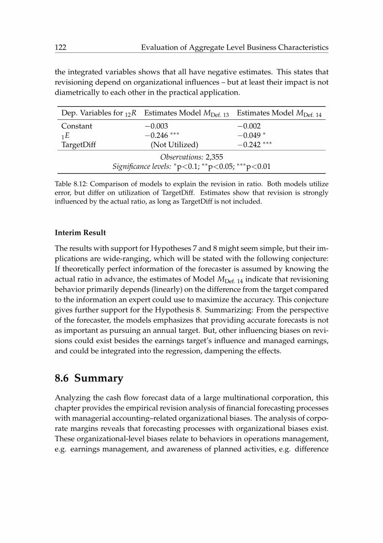
122 Evaluation of Aggregate Level Business Characteristics
the integrated variables shows that all have negative estimates. This states thatrevisioning depend on organizational influences – but at least their impact is notdiametrically to each other in the practical application.
Dep. Variables for 12R Estimates Model MDef. 13 Estimates Model MDef. 14
Constant −0.003 −0.0021E −0.246 ∗∗∗ −0.049 ∗
TargetDiff (Not Utilized) −0.242 ∗∗∗
Observations: 2,355Significance levels: ∗p<0.1; ∗∗p<0.05; ∗∗∗p<0.01
Table 8.12: Comparison of models to explain the revision in ratio. Both models utilizeerror, but differ on utilization of TargetDiff. Estimates show that revision is stronglyinfluenced by the actual ratio, as long as TargetDiff is not included.
Interim Result
The results with support for Hypotheses 7 and 8 might seem simple, but their im-plications are wide-ranging, which will be stated with the following conjecture:If theoretically perfect information of the forecaster is assumed by knowing theactual ratio in advance, the estimates of Model MDef. 14 indicate that revisioningbehavior primarily depends (linearly) on the difference from the target comparedto the information an expert could use to maximize the accuracy. This conjecturegives further support for the Hypothesis 8. Summarizing: From the perspectiveof the forecaster, the models emphasizes that providing accurate forecasts is notas important as pursuing an annual target. But, other influencing biases on revi-sions could exist besides the earnings target’s influence and managed earnings,and could be integrated into the regression, dampening the effects.
8.6 Summary
Analyzing the cash flow forecast data of a large multinational corporation, thischapter provides the empirical revision analysis of financial forecasting processeswith managerial accounting–related organizational biases. The analysis of corpo-rate margins reveals that forecasting processes with organizational biases exist.These organizational-level biases relate to behaviors in operations management,e.g. earnings management, and awareness of planned activities, e.g. difference

Evaluation of Aggregate Level Business Characteristics 123
from target, and lead to systematic biases in forecast revisionsing processes. Re-sults indicate that including organizational biases into accounting is the key toexplain results in aggregate level forecasting.
The empirical analysis of cash flow forecasting in the sample corporation con-firms that the relation between individual bias and accuracy is indeed ambigu-ous. The thesis argues that organizational issues—such as the pursuit of annualreturn targets—introduce organizational-level bias that distorts cognitive biasand explains such counter-intuitive relations. Separating the biases and deter-mining when organizational bias can be expected to distort the diagnosis of indi-vidual bias helps to prevent misinterpretation and rethink organization structure.
In this research, two research gaps were addressed: First, providing insightsinto corporate invoice forecast and revision processes and, second, uncoveringsystematic effects and biases on the aggregate level, where hedging takes place.
Implications on Hedging, Management, and Innovation
For corporations, it is important to understand how organizational business pre-requisites may affect forecasting accuracy in order to decrease hedging costs.In particular, risk management must incorporate planning figures and earningsmanagement to some degree to reach an unbiased perspective. Otherwise, thebiased perspective would impair risk management and hedging activities. Evenif netting effects take place, with positive invoices (II) canceling the effect of neg-ative invoices (IR), the influence of the findings must not be underrated. In par-ticular skewed distributions of invoices would create additional risks or costs forunnecessary hedging. However, the three biases (ratio difference from planningtargets, information concealment, and organizational goals) seem to influence theexperts’ forecasts.
From a managerial perspective, the results provide new insights into how or-ganizational biases influence the purpose of the forecasting task. The endeavorto align forecasts to target figures determines how revisions are made. The ac-curacy and the forecast quality become less important for the human forecastersthan other external and organizational influences. This does not mean that thehuman forecasts have a bad accuracy per se. The analyses revealed that reachingthe target does not conflict with accurate forecasting for the revision behavior. Butaligning the goal of forecasting for individuals to the corporation’s goals seemsto be beneficial. As a result, organizations that want accurate forecasts for in-voice margins from managers should consider motivating purposeful forecasts,i.e. with incentives for forecasters.
In sum, the findings bridge the gap between forecasting research and organiza-
124 Evaluation of Aggregate Level Business Characteristics
tional biases within management research for digital innovation in corporations.The results provided are relevant to corporate leadership, management strate-gies, information technology, and business analytics. Altering the understandingof “the goal of forecasting”, corporate leaders can iteratively measure the impactof a managerial incentive system and build strategies to change organizationaldependencies. For instance, to improve awareness of upcoming earnings man-agement activities, the information might be communicated to the forecasterswith an information system. Business analytics benefits from the informationprovided, as forecast correction services could incorporate dependencies storedin the information system in order to improve the forecast accuracy.
Scope of Business Context
The combination of incentivization, earnings management, and organizationalplanning (organizational biases) leads to forecast revisions most likely dependingon the business context. The pursuit of annual return targets and forecast accu-racy can be relevant in many companies. In case of another structure or differentbusiness model, the dependencies might look different. Also, it seems likely thatother business aspects exist, which additionally biases forecasts.
Business aspects beyond corporate financial responsibilities can provide in-sights to understand interlinks to organizational structures. For example, self-governing departments can have serious implications for corporations, as de-partments’ independence provides no obvious reason to align to corporate goals– besides benevolence. Also, it seems likely that other organizational aspectsexist, such as country-specific tax avoidance. Tax avoidance might affect eachsubsidiary differently by defining upper borders for ratios that subsidiaries mustnot reach. These aspects can be accounted in correction approaches too, but thisthesis can not examine and cover all possible organizational influences.
Correction Opportunities
Improvement processes of corporate risk assessment have an essential need ofunderstanding interlinks of organizational and individual structures, especiallybeyond the organizational borders of the corporation. An approach for improve-ment should account for all relevant organizational levels, and besides takingmanagerial actions, future research work might reveal alternatives. Additionalcorporation wide research and documentation in the meetings, wherefrom effectsmight derive, possibly shows a solution how to identify future, unknown orga-nizational biases. The analyzed organizational target bias and further measure-

Evaluation of Aggregate Level Business Characteristics 125
ment of so far unknown biases might disclose the latent motivations of forecastsin detail. It is concluded that the knowledge of these biases, together with thepredictive value for decision support systems, drives subsequent forecast correc-tion approaches to retrieve highly accurate forecasts for accounting informationsystems. The effort might be high, but the resulting opportunities seem to be evenhigher.

Chapter 9
Evaluation of Predictive Value
This chapter presents the empirical results for prediction analysis. These con-sist of the out-of-sample results on individual and aggregate level, analysis
of error distribution, t-test evaluation, correlation analysis for weak efficiency, inparticular revision and error analysis, and analysis of the extended weak effi-ciency with an examination of the underlying numbers. The chapter concludesby a summarizing interpretation of the results.
9.1 Predictions on Individual Level
9.1.1 Correction: Anchoring and Adjustment
The two models for lead times t = 1 base on MEqu. 5.1, which are exhibited inTable 7.7. They state that the explained variance is below 1 % for each model,questioning whether the models can be applied successfully for statistical debi-asing. The results in Table 9.1 show the respective out-of-sample evaluation whenapplying both models (positive and negative) to correct forecasts.
Overall, the correction model lead to a low mean out-of-sample error reduc-tion compared to the original expert forecasts of 0.29 %. This result states, forexample, an error of one million Euro would be reduced by 2,900 Euro only. Withnetting effect the mean error improvement on net foreign exposure volumes isexpected to be further reduced, questioning if the impact of the model in compar-ison to other forecast correction models is high enough to justify the deployment.However, the extent of improvement varies strongly by month, with error evenincreasing when applying the correction in months 1 and 2 (January and Febru-ary). With regard to the low explained variance, this result indicates that differentbiases might exist that are differently pronounced over the months of a year. Forinstance, further analyses for earnings management at the end of the year couldreason the differences in model performance.
127
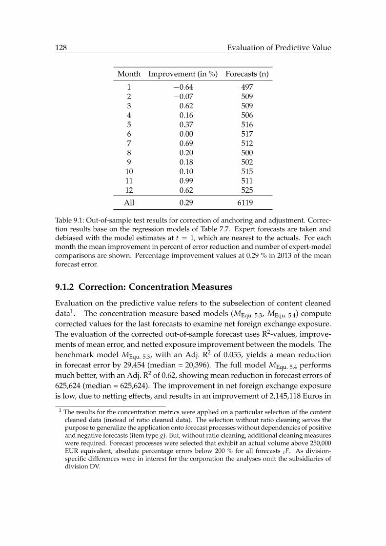
128 Evaluation of Predictive Value
Month Improvement (in %) Forecasts (n)
1 −0.64 4972 −0.07 5093 0.62 5094 0.16 5065 0.37 5166 0.00 5177 0.69 5128 0.20 5009 0.18 502
10 0.10 51511 0.99 51112 0.62 525
All 0.29 6119
Table 9.1: Out-of-sample test results for correction of anchoring and adjustment. Correc-tion results base on the regression models of Table 7.7. Expert forecasts are taken anddebiased with the model estimates at t = 1, which are nearest to the actuals. For eachmonth the mean improvement in percent of error reduction and number of expert-modelcomparisons are shown. Percentage improvement values at 0.29 % in 2013 of the meanforecast error.
9.1.2 Correction: Concentration Measures
Evaluation on the predictive value refers to the subselection of content cleaneddata1. The concentration measure based models (MEqu. 5.3, MEqu. 5.4) computecorrected values for the last forecasts to examine net foreign exchange exposure.The evaluation of the corrected out-of-sample forecast uses R2-values, improve-ments of mean error, and netted exposure improvement between the models. Thebenchmark model MEqu. 5.3, with an Adj. R2 of 0.055, yields a mean reductionin forecast error by 29,454 (median = 20,396). The full model MEqu. 5.4 performsmuch better, with an Adj. R2 of 0.62, showing mean reduction in forecast errors of625,624 (median = 625,624). The improvement in net foreign exchange exposureis low, due to netting effects, and results in an improvement of 2,145,118 Euros in
1 The results for the concentration metrics were applied on a particular selection of the contentcleaned data (instead of ratio cleaned data). The selection without ratio cleaning serves thepurpose to generalize the application onto forecast processes without dependencies of positiveand negative forecasts (item type g). But, without ratio cleaning, additional cleaning measureswere required. Forecast processes were selected that exhibit an actual volume above 250,000EUR equivalent, absolute percentage errors below 200 % for all forecasts tF. As division-specific differences were in interest for the corporation the analyses omit the subsidiaries ofdivision DV.

Evaluation of Predictive Value 129
comparison to the benchmark model.The resulting exposure improvement of the full model is in magnitude an ac-
ceptable high volume, but relatively speaking, the corrected part counts still forless than 0.1 % of the overall net foreign exposure in the out-of-sample period.Further, the forecast error is reduced by less than 0.1 % of the expert exposure er-ror. Despite the explained variances of the concentration models were very high,these figures clearly motivate the analyses for the aggregate corrections.
9.2 Predictions on Aggregate Level
9.2.1 Forecast Correction
The results of the aggregate correction are presented in Table 9.2. The table showsthe date of the month and the amount of ratio forecasts for each month in 2013.Further the table exhibits the aggregated forecast error of the expert forecast (M∅)and model predictions (MBasic and MOrga). The last two columns show the per-centage improvement of the models in comparison to the baseline M∅.
Data Descriptive Forecast Error Improvement (in %)
Date Amount M∅ MBasic MOrga MBasic MOrga
01/2013 58 18.77 18.01 18.40 4.0 % 2.0 %02/2013 60 18.11 15.11 14.38 16.6 % 20.6 %03/2013 60 16.79 14.74 10.86 12.2 % 35.3 %04/2013 60 16.15 14.82 9.66 8.2 % 40.2 %05/2013 61 16.59 15.42 9.25 7.1 % 44.3 %06/2013 61 16.30 15.75 8.34 3.4 % 48.8 %07/2013 61 16.84 15.38 7.91 8.7 % 53.0 %08/2013 61 17.30 15.41 7.39 10.9 % 57.3 %09/2013 61 18.51 16.58 7.35 10.4 % 60.3 %10/2013 63 17.41 16.67 7.28 4.3 % 58.2 %11/2013 63 17.79 15.95 7.10 10.3 % 60.1 %12/2013 63 17.61 15.77 7.05 10.4 % 59.9 %
Table 9.2: Out-of-sample test results for the forecast ratios of experts, the basic statisticalmodel, and the organizational model. Out-of-sample test covers the forecast correctionin 2013. Cumulative absolute forecast error for expert forecast M∅, MBasic, and MOrga areshown. MOrga predictions have the lowest forecast error (7.05 in December) compared toM∅ and MBasic predictions. Percentage improvement compares the specific model errorto the baseline of expert error. The improvements at the end of the year show that MOrgareduces error by 59.9 %, which is better than MBasic with 10.4 %.

130 Evaluation of Predictive Value
The organizational information to reach the assumed target ratio clearly relatesto the forecast error of Model MOrga, as comparison for column four and fiveshows. Approaching the end of the fiscal year the Model MOrga reduces the ag-gregated forecast error to 7.05, while expert M∅ and Model MBasic error is stablein a disquieting high way. Considering that 100 % is the full opportunity forimprovement as the resulting error would be equals zero, the result shows theadvantage of the organizational information. In January the MBasic has an ad-vance of two percent, but for all other months MOrga outperforms the foresaidmodel. The results show that percentage improvement of the models with solelystatistical information reduces the expert error up to 16.6 % in February, while themodels that considers business key figures performs with up to 60.3 % improve-ment in September.
The paired t-test based on the monthly improvements of Model MBasic andModel MOrga (comparison of the last two columns in Table 9.2) provides the fol-lowing statistics: t = 6.7299, df = 11, p-value = 3.243e-05. The statistics evidencethat the results in the out-of-sample period are significant at the 0.01 % level,supporting Hypothesis 9.
9.2.2 Error Distribution of Forecast Correction
The error analysis starts with a summary of the forecast error 1E, shown in theTable 9.3. These numbers provide the first support for the superior debiasingperformance of MOrga. Quantiles and median of the error are highly improved incomparison to M∅ and MBasic.
Approach Min. 1st Qu. Median Mean 3rd Qu. Max.
M∅ −1.000 −0.239 −0.038 −0.068 0.125 1.000MBasic −0.651 −0.201 −0.021 0.001 0.216 0.824MOrga −0.681 −0.129 −0.004 −0.003 0.096 0.926
Table 9.3: Error quantiles of 1E for the forecasts of experts, the basic statistical, and theorganizational model.
The Figure 9.1 shows important information for the error quantiles of the fore-casts utilizing a violin plot. This figure provides further support for the perfo-mance of MOrga by the 1E measure. The organizational model outperforms thestatistical model especially for the 1. quartile (∆ = 0.072), median (∆ = 0.017),and 3. quartile (∆ = 0.120). Furthermore, the lower and upper whiskers areimproved. Only for minimum, maximum, and for mean error (∆ = 0.002) thestatistical model seems beneficial.
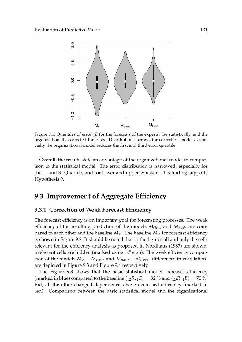
Evaluation of Predictive Value 131
−1.
0−
0.5
0.0
0.5
1.0
M0 MBasic MOrga
Figure 9.1: Quantiles of error 1E for the forecasts of the experts, the statistically, and theorganizationally corrected forecasts. Distribution narrows for correction models, espe-cially the organizational model reduces the first and third error quantile.
Overall, the results state an advantage of the organizational model in compar-ison to the statistical model. The error distribution is narrowed, especially forthe 1. and 3. Quartile, and for lower and upper whisker. This finding supportsHypothesis 9.
9.3 Improvement of Aggregate Efficiency
9.3.1 Correction of Weak Forecast Efficiency
The forecast efficiency is an important goal for forecasting processes. The weakefficiency of the resulting prediction of the models MOrga and MBasic are com-pared to each other and the baseline M∅. The baseline M∅ for forecast efficiencyis shown in Figure 9.2. It should be noted that in the figures all and only the cellsrelevant for the efficiency analysis as proposed in Nordhaus (1987) are shown,irrelevant cells are hidden (marked using "x" sign). The weak efficiency compar-ison of the models M∅ − MBasic and MBasic − MOrga (differences in correlation)are depicted in Figure 9.3 and Figure 9.4 respectively.
The Figure 9.3 shows that the basic statistical model increases efficiency(marked in blue) compared to the baseline (12R, 1E) = 92 % and (23R, 1E) = 70 %.But, all the other changed dependencies have decreased efficiency (marked inred). Comparison between the basic statistical model and the organizational

132 Evaluation of Predictive Value
x
x
x
x
x
x
x
x
x
x
x
x
−1 −0.8 −0.6 −0.4 −0.2 0 0.2 0.4 0.6 0.8 1
4E
3E
2E
1E
45R
34R
23R
12R
4E
3E
2E
1E
45R
34R
23R
12R
Figure 9.2: Correlation of revisions with errors and revisions of experts, without any cor-rection (baseline model M∅).
0
0
0
0
0
0
0
0
0
0
−0.9
−0.19
0.7
0.92
0
0
0
−0.72
0
0
−0.85
0
−0.83 0
x
x
x
x
x
x
x
x
x
x
x
x
4E
3E
2E
1E
45R
34R
23R
12R
4E
3E
2E
1E
45R
34R
23R
12R
Figure 9.3: Percentage improvement in correlation of the basic statistical model MBasicover the baseline model M∅ (positive numbers exemplify the improvement).

Evaluation of Predictive Value 133
0
0
0
0
0
0
0
0
0
0
0.73
0.16
0.63
0.56
0
0
0
0.57
0
0
0.06
0
0.19 0
x
x
x
x
x
x
x
x
x
x
x
x
4E
3E
2E
1E
45R
34R
23R
12R
4E
3E
2E
1E
45R
34R
23R
12R
Figure 9.4: Percentage improvement in correlation of the organizational model MOrgaover the baseline model MBasic (positive numbers exemplify the improvement).
model in Figure 9.4 shows an increase of efficiency relative to MBasic by 56 %for the final forecast. More remarkable, the whole forecasting revision process ismore efficient (see (12R, 23R), (12R, 34R), and (12R, 45R)).
Empirical results show that correction techniques can utilize organizational ef-fects to improve forecast efficiency. The reduction of inefficient pattern showsthat correction techniques with organizational forecast debiasing is superior tobasic statistical approaches.
The results for the correlation of (12R, 1E) are not significant after correctiondue to the high efficiency, but the details are shown in Table 9.4. The Spearmancovariance for the approaches states that revisions and errors have a lower jointvariability. The organizational model has a positive covariance, while the statis-tical model has a negative covariance with a higher magnitude. The table showsthat MOrga increases standard deviation for the revision, but standard deviationreduces for the error. It is arguable with these numbers that the correction of theorganizational model focuses with meaningful revisions on the reduction of theerror, while the the correction of the basic statistical model focuses on changingthe error with minor corrections. The results imply that MOrga enables future ap-proaches to detect other, currently unknown biases to be identified and removed.

134 Evaluation of Predictive Value
Approach Covariance(12R,1E) Std.Dev.(12R) Std.Dev.(1E)
M∅ (Baseline) −246092.58 0.24 0.34MBasic (Statistical) −20360.87 0.21 0.28MOrga (Organizational) 8968.19 0.28 0.20
Table 9.4: Spearman correlation details of the last revision and final error for forecastratios of the experts, the statistically, and the organizationally corrected forecast ratios.MOrga exhibits the highest standard deviation for revision while having the lowest stan-dard deviation for error.
Interim Result
The results state Hypothesis 11 in the terms of Nordhaus’s weak form forecastefficiency. The empirical results show that forecasts correction based on orga-nizational information can improve forecast efficiency of (12R, 1E) by 56 % incomparison to a statistical approach. The reduction of inefficient pattern showstatistics arguing for forecast correction that rely on organizational biases (stan-dard deviation of error 0.20) instead of basic statistical approaches that harmforecast efficiency (standard deviation of error 0.28). Overall, the results stateseveral advantages of the organizational model in comparison to the basic sta-tistical model. First, Hypothesis 10 is supported. The purely statistical modeldecreased efficiency in five of seven cases (Figure 9.3). Second, in the sense ofNordhaus the organizational model for debiasing improves forecast efficiency for(12R, 1E). Moreover, the efficiency of the entire forecast process is improved (Fig-ure 9.4), supporting Hypotesis 11. Third, highly improved efficiency for MOrgaover MBasic in (12R, 1E) and (23R, 1E) and the advantage of meaningful revisionsinstead of pure error reduction (Table 9.4), which supports Hypothesis 12.
9.3.2 Correction of Extended Weak Forecast Efficiency
The extended weak forecast efficiency of the original forecasts M∅ and the result-ing ratio prediction of the correction models MBasic and MOrga are compared toeach other. The results of the different predictions are presented in Table 9.5. Theupper part of the table shows the correlations between the last revisions with revi-sions and errors of M∅, MBasic, and MOrga. The lower part shows the correlationsbetween the last error with revisions and other errors. The performance of theorganizational model will be analyzed in the following explanations of extendedweak forecast efficiency.

EvaluationofPredictive
Value
135
Metric Approach 45R 34R 23R 12R 5E 4E 3E 2E
Revision (2) Timing (3)
12R M∅ −0.13∗∗∗ −0.03∗∗ −0.24∗∗∗ 1.00 0.07∗∗∗ 0.15∗∗∗ 0.15∗∗∗ 0.35∗∗∗
12R MBasic −0.22∗∗∗ −0.06∗∗∗ −0.44∗∗∗ 1.00 0.06∗∗∗ 0.19∗∗∗ 0.22∗∗∗ 0.55∗∗∗
12R MOrga −0.10∗∗∗ −0.05∗∗∗ −0.36∗∗∗ 1.00 0.38∗∗∗ 0.45∗∗∗ 0.50∗∗∗ 0.79∗∗∗
Purpose (1) Impact (4)
1E M∅ 0.02 0.01 −0.10∗∗∗ −0.31∗∗∗ 0.59∗∗∗ 0.60∗∗∗ 0.63∗∗∗ 0.71∗∗∗
1E MBasic 0.03∗ 0.02 −0.03 −0.03 0.71∗∗∗ 0.71∗∗∗ 0.74∗∗∗ 0.79∗∗∗
1E MOrga −0.01 0.01 −0.01 0.01 0.50∗∗∗ 0.52∗∗∗ 0.55∗∗∗ 0.58∗∗∗
Note: ∗ p-value < 0.1, ∗∗ p-value < 0.05, ∗∗∗ p-value < 0.01.
Table 9.5: Analysis of correction efficiency for the forecasts of the experts, the basic statistical model, and the organizational model.Results show correlation values and p-value levels of the last revision and the last error in ratio.

136 Evaluation of Predictive Value
Extended Weak Forecast Efficiency: Revision
The upper left part with the first six columns of Table 9.5 shows the relevantfigures for the weak form forecast efficiency concerning revision (Nordhaus’s re-vision dependencies). The model MBasic increases the correlation for all revisionvariables. The model MOrga increases with it’s forecasts the correlation of 12R toall revision variables, except for 45R. When the correlations between the mod-els and the original forecast are compared, the numbers state that MBasic clearlydamages the forecast efficiency the most. MOrga is not beneficial compared to theoriginal forecasts, with one exception the correlation between (45R, 12R). Herethe model improves the forecast efficiency in comparison to the experts. The de-creased correlation between 45R and 12R does make sense due to the fact thatMOrga in particular incorporates figures of the assumed target (and these figuresare at least one year before the current revision). However, MOrga outperformsMBasic in all these correlations. From these numbers it can be concluded that it isdifficult but possible to improve forecast efficiency by models (besides error opti-mization). Overall, the organizational model is superior to the purely statistical.
Extended Weak Forecast Efficiency: Timing
The insight for the timing is provided in the upper right part of the Table 9.5(columns 5E to 2E). Here, high values are a positive result as the subsequent revi-sion 12R should increase in magnitude to be able to adjust errors. The magnitudeof the correlations in the columns 5E to 2E hint to the fact that the biasing pat-tern is also existing in earlier forecasts (and their errors). It is argueable that theunderlying pattern that a model should correct (for MBasic and MOrga) increasesin influence with decreasing lead time from the earliest forecast with error 5Euntil 2E. Therefore the thesis argues that MBasic corrects (indicated by positivecorrelation) a pattern that exists less in the beginning (value 0.06) and mainly inthe end (value 0.55) of the forecasting process. In contrast, the model MOrga cor-rects (indicated by positive correlation) an underlying pattern that is existing andmore important during the whole forecasting process (correlation values of 0.38up to 0.79). Altogether, it is expected that MOrga corrects biases that exist for alonger time compared to the biases that MBasic corrects. These results supportProposition 9.
Extended Weak Forecast Efficiency: Purpose
In the lower left part of the table the shown figures are important regarding thepurpose of the models. The only figures relevant to Nordhaus can be found in
Evaluation of Predictive Value 137
the sixth column of the lower part of the table, the correlation between 12R and1E. Here, the models strongly improve the correlation from −0.31 to −0.03, re-spective to 0.01. As both models optimize the error, the results are as expected.Further, the error correlation of both models are compared to those of the expert.The results show that for the revision-columns (45R to 12R) the correlation is re-duced (in magnitude and p-value). The figures state that both models serve theirpurpose to reduce the relation between the last revision and error, making theforecasts more efficient. One exception is Cor(45R,1E), which states that the errorof the prediction of MBasic is less efficient to the previous year adjustments, whileMOrga is still efficient.
Extended Weak Forecast Efficiency: Impact
The error-columns (5E to 2E) in the lower right part exhibits an advantage withregard to the impact of the model MOrga. Here, lower correlation-numbers statethat the error of the model is less dependent on previous errors, which is a desiredresult of a bias correction model. The MOrga reduces the inherent organizationalbias within the original forecasts and the result shows that the error correlationreduces (e.g. see column 2E, M∅: 0.71 vs. MOrga: 0.58). The example of an unde-sired outcome is visible for MBasic (e.g. see column 2E, M∅: 0.71 vs. MBasic: 0.79).Moreover, MBasic increases the correlation between all the errors of the entire fore-cast process in comparison to M∅. This means a high error of the expert in anearly phase (such as 5E) probably results in an high error of the statistical modelprediction (1E). The model MBasic is therefore highly dependent on the input ofM∅, and MOrga is less dependent (column-wise perspective). Even more inter-estingly, the magnitude of error-correlations of model MOrga is below the expertM∅, stating that the utilization of organizational information leads to higher in-dependence of forecasts (row-wise perspective). The underlying approach of thestatistical model obviously optimize the error of the forecast, leaving the impor-tant bias mostly unchanged within the forecasts, while the organizational modelfocuses especially on an important bias. That explains the different model re-sults. However, the results do not support Proposition 10, even if the modelsexhibit correlation values for 2E and 1E, which show that the statistical modelrequires further improvements to at least reach the results of the organizationalmodel (correlation values of MBasic > M∅ > MOrga).

138 Evaluation of Predictive Value
Interim Result
Hypothesis 12 is supported in the extended weak forecast efficiency analyses thatshow the superiority of organizational models for debiasing, namely the revision,the timing, the purpose, and the impact on how the model corrects the expertforecasts.
Overall, the results state several advantages of the organizational model MOrgain comparison to the statistical model MBasic. First, in the sense of Nordhausthe organizational model improves forecast efficiency for Cor(12R, 1E) and hasno deficits for Cor(45R, 1E) (Ext. Efficiency: Purpose). Second, in the sense ofNordhaus the correction improves the forecasts, especially for Cor(45R, 12R) (Ext.Efficiency: Revision). Third, the underlying pattern upon the correction is basedis important even at the early stages of the forecast process (Ext. Efficiency: Tim-ing). Fourth, improvements of MOrga make the error less dependent from previ-ous errors and from expert inputs (Ext. Efficiency: Impact). The result supportHypothesis 13.
9.4 Summary
Improving information systems and decision support tools can help to reducehedging costs and the managerial workload (with regard to the manual identi-fication of forecasts items that need revising). The empirical results of forecastcorrection techniques were comprehensive. This has led to starting a new projectwith the research partner, the corporation that provided the analyzed data, toutilize the model predictions with organizational debiasing and to automaticallycheck the expert’s validity of ratio forecasts within a forecast support system. Theorganizational model debiases at an aggregate level, where business reasons mat-ter. Overall, the results show that consideration of business key figures makes iteasier to identify on an aggregate level the most beneficial work packages of fore-casts that need revisions.
Predictive Value: Individual Level
The analyses on individual level cash flow forecasts associated the revisions pat-tern to forecast accuracy. The metrics used to improve the forecasts in the revisionprocesses show that these have low explanatory power (below 1% for correctionmodels based on A&A) and high explanatory power (above 60% for correctionmodels based on concentration measures). However, the out-of-sample test re-sults suggest that by considering these patterns, the improvement of net foreign

Evaluation of Predictive Value 139
exchange exposure is marginally better than the expert forecasts. In both casesless than 0.3% of the expert error could be improved, which suggests to analyzepredictive value of aggregate level.
Predictive Value: Aggregate Level
Information systems with services for decision support systems benefit from theinsights provided. The empirical analyses show that business information pro-vides meaningful key figures for predictive purposes. Explicitly, forecast cor-rection approaches that incorporate organizational dependencies (EBITDA proxyinformation) can highly improve forecast accuracy.
The empirical results on ratio show that considering organizational objectivesfor debiasing techniques can strongly improve forecast accuracy. The total cor-rectable expert error is reduced by up to 60 % for all forecasts of a month, pro-viding better decision support for managers, and reducing the personnel effortto determine forecasts with suspicious pattern that are unaligned with organiza-tional structures.
Besides ratio-level correction, utilizing ratio information for correcting individ-ual forecasts is should be considered. By improving ratio forecasts the error of thenet foreign exposure may theoretically improve by up to 60 %, which requires amapping function from ratio of accumulated invoices issued and invoice receivedto the accumulated difference between them for each month (net exposure). Insum, the results provide out-of-sample evidence of organizational influences andmethodology to analyze fewer issues by identifying those that really matter.
Aggregate Level Efficiency Improvement
For the forecasting community the results might reinforce the link between ex-ploratory data analysis and forecast correction. Exploring data can actually pro-vide essential information. I’d like to underline that the results were not achievedwith a neural network, a random forest, or a complex machine learning algo-rithm. Instead, the results are achieved with a simple linear regression models.
The importance of exploratory data analysis is underlined as data and businessunderstanding additionally allows a differentiation between biases with patternand errors, stated by aggregate level efficiency. From the perspective of forecastresearcher it is important to understand in which way business-related organi-zational influences may affect forecasts and, indirectly, correction models. In thecase of cash flow forecasts in a corporate setting one important bias is the per-centage margin target, as these might provide incentivization to alter forecasts

140 Evaluation of Predictive Value
and actuals of cash flows. The underlying value of this organizational informa-tion on ratios in terms of forecast efficiency. The analysis showed that efficiencyincreases for the whole process when such information is integrated into a cor-rective model.
Extended Forecast Efficiency Analysis
An important theoretical result is the conclusion that the different results for cor-rective models may be inherent to each approach. This thesis contributes with ap-plying the developed approach to test for the extended weak forecast efficiency.This approach states that a basic statistical model mainly tries to optimize the se-lected component (e.g., the error), while an organizational model tries to reducethe bias itself.
Thus, the organizational model provides the possibility to identify further un-known biases. Even if the debiasing with a single organizational model does notachieve a high error decrease, it is possible to identify and correct further biaseswith a second subsequent model. Finally, a subsequent set of models for the mostimportant organizational biases will definitely increase the forecast accuracy. Un-derstanding the error components for correction approaches is important. Whena forecaster distinguishes the signal from the noise, the error should decrease bythe way or making predictions more confident.
Despite the fact that the organizational model has two flaws in efficiency – in(12R, 34R) and (12R, 23R) – the model MOrga outperforms the expert M∅ in all otheraspects of extended forecast efficiency. Furthermore, MOrga outperforms MBasicin every aspect. These results state that organizational information is essentialfor forecast correction, while the extended weak efficiency analysis provides aframework to understand the differences in correction approaches.

Part IV
Finale

Chapter 10
Conclusion and Outlook
10.1 Summary
Forecast efficiency theory is widely used to investigate judgmental forecaststhat regularly turn out to be inefficient in terms of weak form forecast effi-
ciency. Influences that lead to individual level biases are usually associated withsuch inefficiencies. However, influences can also lead to organizational-level bi-ases. This is why particular importance should be given to improve the under-standing of the context of forecast processes.
This thesis contributes to the literature with analyses of forecast efficiency, indi-vidual biases, organizational biases, forecast correction, and the links in between.Based on corporate data for judgmental cash flow forecasts, this works showedthat isolated tests for biases and forecast efficiency must be interpreted with spe-cial care. The analyses revealed a need for an integrative view to determine andinterpret the respective biases appropriately.
The analyses provided evidence for the pursuit of annual returns targets inrelation to earnings management, which not only reveals predictable patterns ofhow the ratios of accumulated cash inflows and cash outflows are adjusted overtime, but also provides reasonable explanations for phenomena that contradictefficiency theory. Explicitly, some of the inefficiencies in the data were found tobe associated with improved forecast accuracy, which could be explained by theknowledge of earnings management.
While it is likely that earnings management in pursuit of annual returns tar-gets will be relevant in many business contexts, there might well be additionalorganizational biases at play. But in practice, however, non-disclosed volumesof presumed earnings targets and missing direct observations of earnings man-agement or other potentially bias-related activities make forecast analyses andmodel based correction truly challenging. With such information available, itwould become much easier to unravel the effects of different biases on forecast-
143
144 Conclusion and Outlook
ing processes. Separating the biases and determining when organizational biasescan be expected to distort the diagnosis of individual biases helps to prevent mis-interpretations and rethink organization structure.
Despite the potential causes of the predictability of the cash flow forecasts at thecumulative ratio level, the results indicate an enormous potential for improvingthe longer–term cash flow forecasts and corporate risk assessment that uses theforecast data of the financial system. Specifically, forecast difference from targetis the key to explaining results in corporate cash flow forecasting.
In the following part of this chapter, the research results are summarized anddiscussed in the context of the corporate forecast and its implications for the mainresearch questions. To conclude, further future questions will be outlined on thebasis of the thesis.
10.2 Contributions
The objective of this thesis was to investigate forecast efficiency, different biasesand forecast correction, and their relation in the context of forecast processes.For empirical forecasts in intra-corporate financial planning, this thesis showedthat biases exist already at the level of individual forecasts but that forecastsare influenced in particular by organizational biases. Existing inefficiencies atthe organizational level underline these dependencies. Based on research ques-tions 1 – 3, the individual level was investigated. The aspects of the aggregatelevel were analyzed based on research questions 4 – 6. The research questionsdiscussed in Section 1.2 are summarized as:
RQ 1. Forecast Efficiency — Revision ProcessRQ 2. Forecast Efficiency — Efficiency HypothesisRQ 3. Revision Process — Anchoring & AdjustmentRQ 4. Revision Process — Organizational InfluenceRQ 5. Organizational Influence — Forecast CorrectionRQ 6. Forecast Correction — Forecast Efficiency
As a result of my research, I have answered these six complex research ques-tions as follows: For research question 1, it can be summarized that the corpo-rate forecasts analyzed do not exhibit weak efficiency and that, hence, forecastcorrection potential is available. Save for a few exceptions, forecast horizons areassociated positively with the forecast errors. Based on research question 2, an ap-proach to evaluate the efficiency hypothesis was introduced. The results obtainedlead to a rejection of the efficiency hypothesis for the corporation’s consolidated

Conclusion and Outlook 145
cash flow data. Further, all violations of the efficiency hypothesis were associatedto organizational influences. Regarding research question 3, this thesis has iden-tified and described different patterns of individual biases based on the possibili-ties of identification. Several Bandwidth Models and concentration measures arepointed out as metrics that can map more complex relationships than the usualmetrics. The forecast correction advantages were pointed out for the respectivemodels. Research question 4 can be confirmed on the aggregate level. Here, orga-nizational biases exist in terms of the return ratio relative to annual earnings tar-gets. The dependencies on annual targets, revisions, and forecast errors evaluatedin addition gave deep insight into existing forecasting processes. Research ques-tion 5 was answered through evaluation of aggregate level forecast correction,where correction of organizational biases provides impressive improvements, inparticular in comparison to purely statistical approaches. Finally, research ques-tion 6 was answered by means of an efficiency analysis of the corrected forecastsfrom an organizational and a standard statistical correction method. This thesis’sresearch was able to show that standard statistical corrections focus on the errorreduction, are disadvantageous for the efficiency of forecast processes, and thatorganizational corrections outperform the purely statistical corrections in all as-pects of extended weak forecast efficiency. The full list of research questions andtheir results are exhibited in Appendix A.
10.3 Future Outline
At present, efficiency theory is applied mainly showing that markets and fore-casting processes are not efficient, i.e. that there exists improvement potential.The question as to what type of corrections are suitable and necessary to achieveadvantages for forecasting processes, among others, was pointed out in this thesison biases and forecast efficiency in corporate finance. Summarizing: Improvedaggregate model forecasting revealed efficiency emendation. This work providesa basis for future research e.g., on forecast efficiency, bias extraction, implicationsfor managers, and forecast correction, that will follow.
10.3.1 Forecast Efficiency
Efficiency at Different Aggregation Levels: Over Time
Efficiency is fundamental in its theory and, hence, can provide meaningful state-ments. However, there are no basic studies on the statistical properties of weakforecast efficiency. Research, therefore, should focus in particular on assessing
146 Conclusion and Outlook
the impacts of aggregation for efficiency e.g., of aggregation over time (insteadof over different subsamples of the categorical features of a dataset). I expectthat a coarser aggregation of units will reveal fundamental changes in forecastefficiency in the context of seasonal aspects.
Efficiency Related to Information
Besides the above, linking of information on efficiency is an aspect to be consid-ered. If already known and important information is newly integrated into pro-cesses, this should clearly prove the absence of efficiency. A formal analysis andderivation of this relationship would be desirable. Moreover, the understandingof weak efficiency should be changed in such a way that the concept of efficiencydoes not focus on the single points of a forecasting process but on the entire pro-cess, thus enabling a systematic comparison of different forecasting processes asa whole.
Efficiency for Pre-Evaluation of Predictions
In my opinion, the concept of efficiency could be used also for analyzing forecastsin a pre-evaluation step. The research question would be how far, in a forecastingprocess, the forecasts of a correction model must be independent from one an-other. To my mind, independence of forecasts should be guaranteed under the as-sumption of a random walk, if all corrections concerning content (e.g., organiza-tional debiasing) have been carried out. Such analyses can be applied before thereal reference values exist and would, so to speak, be out-of-sample evaluationswithout the need of real values. However, at least as regards error minimization,corrected forecast revisions should have the same efficiencies as the revisions ofthe realizations. From the theoretical and practical points of view, it would beparticularly interesting to analyze the dependencies of the pre-evaluation resultsand the resulting real forecast errors.
10.3.2 Formalized Bias Extraction
As is pointed out in the Chapter 4.2.1, important relationships within forecastingprocesses can be identified by means of efficiency analyses and expert knowl-edge of extremely complex issues. Automation of this method in order to matchthe expert knowledge with the advantageous or disadvantageous efficiencies inforecasting processes could improve dealing with the practical questions and ad-vance research, in particular. This would require to formalize the expert knowl-edge at which point biases are to be expected in the forecast processes. At least
Conclusion and Outlook 147
from the theoretical point of view, the results of such formalization could bematched automatically to the efficiencies in the respective processes. The depen-dencies between the efficiencies and individual information from experts couldserve to evaluate and confirm drawn up and automated models. In particular,this approach provides a possibility of partially automating the research process,which could lead to machine-based research and human scientific work at a newlevel of abstraction.
10.3.3 Managerial Implications
From a practical point of view, two implications for management and processescan be derived directly from this thesis. Forecasting processes must be adaptedaccording to the margin targets, either through improved provision and use ofexisting knowledge (e.g. by central knowledge management of margin definitionand relevance within the respective companies), or by lower incentives within thesubsidiaries or incentives through the corporation from the outside. In practicalterms, this should result in better reconciliation between the participating personsand thus in improvements regarding forecasts and realization values. Moreover,it becomes evident that without expert knowledge, the efficiency results cannotbe put in a context. To consolidate the results, the existing knowledge should bewell documented and explicit incentives should be given for documentation.
10.3.4 Forecast Correction
Correction Methods
Over a long time, attempts have been made to minimize forecast errors indepen-dent of the respective topic. To my mind, this means “improvement of symp-toms” and is at the expense of the different correction methods (e.g., regressionsversus decision trees versus neural networks). The focus on symptoms has ledto diverging views within science and practice and in solitary attempts at find-ing answers to the question as to “which specific algorithm provides lower errorrates”. At the present state of research, where low forecast errors are to be ex-pected and where continuous reliability and stability of forecasts are of particularsignificance, this should not be the only central question anymore, and debiasingshould play a role. Usage of organizational biases to correct the inherent relation-ships is helpful in the case of intra-corporate financial planning. The applicationto debias forecasts from organizational influences would also be interesting forother correction methods and forecasting in other domains.

148 Conclusion and Outlook
Sequential Correction
As a rule, mainly only error metrics are accepted for evaluation of correctionapproaches. Considering the results of this thesis and the possible future im-provements in efficiency theory pointed out above, it suggests itself to comparedifferent sequential correction processes in addition to the individual forecast-ing processes. Assumed that there are two alternative sequential approaches,A(B(data)) or C(D(data)), one could evaluate which correction process (i.e., ABor CD) is more suitable for mapping and correcting the relationships of the con-tents. Moreover, the intermediate results of B(data) and D(data) can be comparedthrough efficiency analysis even if the resulting intermediate results are not ofthe same result type. Inefficient approaches within the sequential (correction)process hence can be identified to show where improvements in such complex(correction) processes can be advantageous.
Bias Correction and Error Reduction
Finally, I would like to recommend to place the focus of scientific research onthe reasons for error corrections. Corrections with statistical methods that par-ticularly aim to reduce errors but not to remove (or reduce) biases must be ques-tioned. Without analyzing or correcting the reasons, correction will always staybehind the symptoms. The forecasting community is recommended not to re-duce the error component by changing forecasts and revisions marginally but toinstead maximize or at least change the forecasts and revisions to an acceptableextent resulting in only marginal errors. The consistency of a high revision willdetermine in how far the forecast result is aligned to the bias pattern. Based onsuch results, an understanding of forecasts and best correction techniques is ob-tained along the way. Overall, consideration of inherent relationships throughmodel-based description and correction can start where errors actually occur. In-stead of placing emphasis on the correction of the symptoms, the technique toremove organizational biases and this thesis promote the correction of the under-lying original reasons.

Part V
Appendix

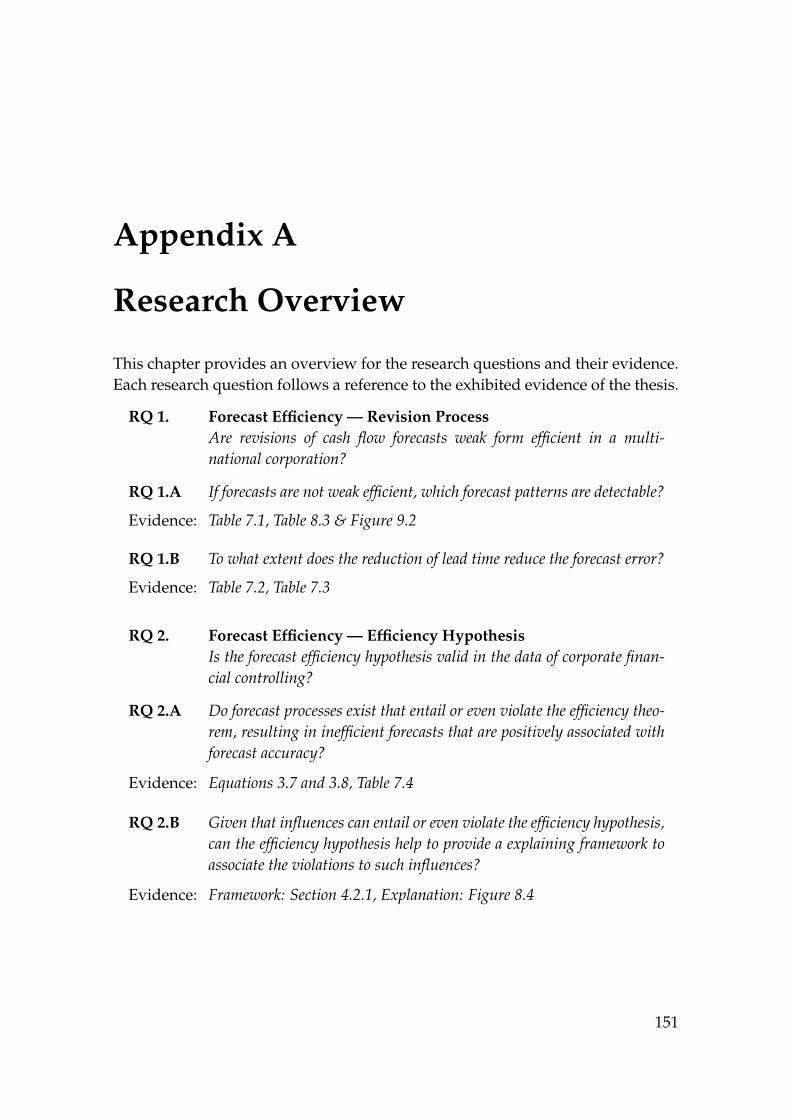
Appendix A
Research Overview
This chapter provides an overview for the research questions and their evidence.Each research question follows a reference to the exhibited evidence of the thesis.
RQ 1. Forecast Efficiency — Revision ProcessAre revisions of cash flow forecasts weak form efficient in a multi-national corporation?
RQ 1.A If forecasts are not weak efficient, which forecast patterns are detectable?
Evidence: Table 7.1, Table 8.3 & Figure 9.2
RQ 1.B To what extent does the reduction of lead time reduce the forecast error?
Evidence: Table 7.2, Table 7.3
RQ 2. Forecast Efficiency — Efficiency HypothesisIs the forecast efficiency hypothesis valid in the data of corporate finan-cial controlling?
RQ 2.A Do forecast processes exist that entail or even violate the efficiency theo-rem, resulting in inefficient forecasts that are positively associated withforecast accuracy?
Evidence: Equations 3.7 and 3.8, Table 7.4
RQ 2.B Given that influences can entail or even violate the efficiency hypothesis,can the efficiency hypothesis help to provide a explaining framework toassociate the violations to such influences?
Evidence: Framework: Section 4.2.1, Explanation: Figure 8.4
151
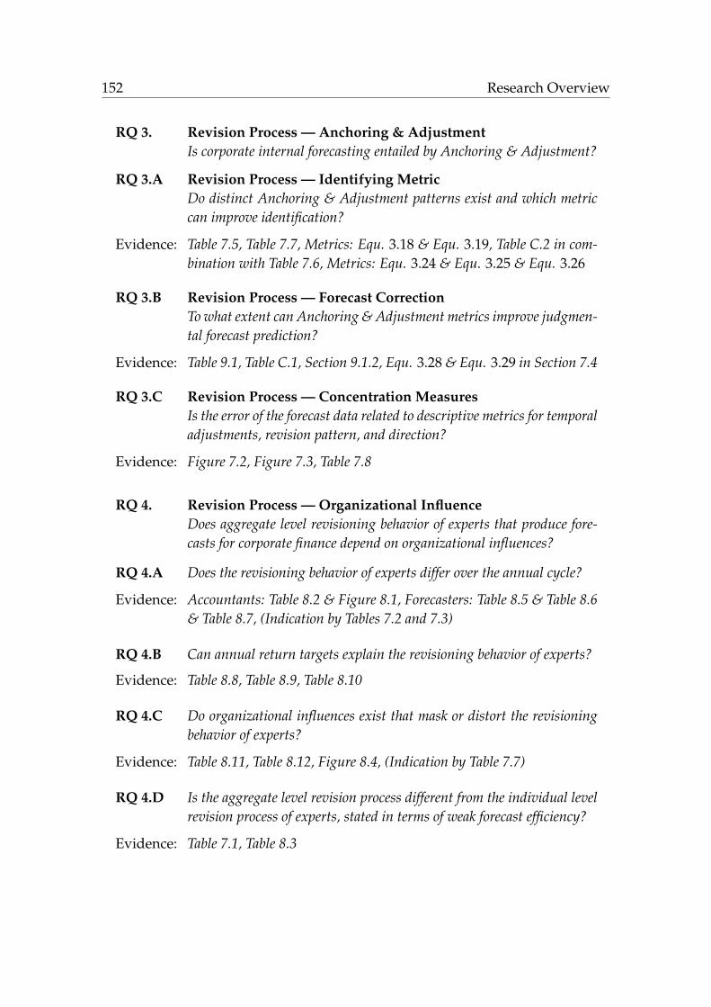
152 Research Overview
RQ 3. Revision Process — Anchoring & AdjustmentIs corporate internal forecasting entailed by Anchoring & Adjustment?
RQ 3.A Revision Process — Identifying MetricDo distinct Anchoring & Adjustment patterns exist and which metriccan improve identification?
Evidence: Table 7.5, Table 7.7, Metrics: Equ. 3.18 & Equ. 3.19, Table C.2 in com-bination with Table 7.6, Metrics: Equ. 3.24 & Equ. 3.25 & Equ. 3.26
RQ 3.B Revision Process — Forecast CorrectionTo what extent can Anchoring & Adjustment metrics improve judgmen-tal forecast prediction?
Evidence: Table 9.1, Table C.1, Section 9.1.2, Equ. 3.28 & Equ. 3.29 in Section 7.4
RQ 3.C Revision Process — Concentration MeasuresIs the error of the forecast data related to descriptive metrics for temporaladjustments, revision pattern, and direction?
Evidence: Figure 7.2, Figure 7.3, Table 7.8
RQ 4. Revision Process — Organizational InfluenceDoes aggregate level revisioning behavior of experts that produce fore-casts for corporate finance depend on organizational influences?
RQ 4.A Does the revisioning behavior of experts differ over the annual cycle?
Evidence: Accountants: Table 8.2 & Figure 8.1, Forecasters: Table 8.5 & Table 8.6& Table 8.7, (Indication by Tables 7.2 and 7.3)
RQ 4.B Can annual return targets explain the revisioning behavior of experts?
Evidence: Table 8.8, Table 8.9, Table 8.10
RQ 4.C Do organizational influences exist that mask or distort the revisioningbehavior of experts?
Evidence: Table 8.11, Table 8.12, Figure 8.4, (Indication by Table 7.7)
RQ 4.D Is the aggregate level revision process different from the individual levelrevision process of experts, stated in terms of weak forecast efficiency?
Evidence: Table 7.1, Table 8.3
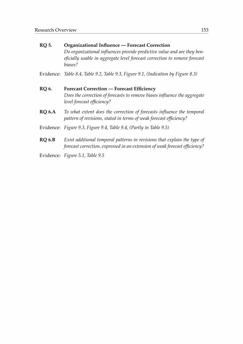
Research Overview 153
RQ 5. Organizational Influence — Forecast CorrectionDo organizational influences provide predictive value and are they ben-eficially usable in aggregate level forecast correction to remove forecastbiases?
Evidence: Table 8.4, Table 9.2, Table 9.3, Figure 9.1, (Indication by Figure 8.3)
RQ 6. Forecast Correction — Forecast EfficiencyDoes the correction of forecasts to remove biases influence the aggregatelevel forecast efficiency?
RQ 6.A To what extent does the correction of forecasts influence the temporalpattern of revisions, stated in terms of weak forecast efficiency?
Evidence: Figure 9.3, Figure 9.4, Table 9.4, (Partly in Table 9.5)
RQ 6.B Exist additional temporal patterns in revisions that explain the type offorecast correction, expressed in an extension of weak forecast efficiency?
Evidence: Figure 5.1, Table 9.5

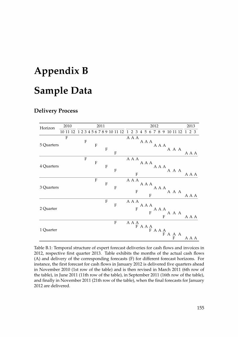
Appendix B
Sample Data
Delivery Process
Horizon 2010 2011 2012 201310 11 12 1 2 3 4 5 6 7 8 9 10 11 12 1 2 3 4 5 6 7 8 9 10 11 12 1 2 3
5 Quarters
F A A AF A A A
F A A AF A A A
F A A A
4 Quarters
F A A AF A A A
F A A AF A A A
F A A A
3 Quarters
F A A AF A A A
F A A AF A A A
F A A A
2 Quarter
F A A AF A A A
F A A AF A A A
F A A A
1 Quarter
F A A AF A A A
F A A AF A A A
F A A A
Table B.1: Temporal structure of expert forecast deliveries for cash flows and invoices in2012, respective first quarter 2013. Table exhibits the months of the actual cash flows(A) and delivery of the corresponding forecasts (F) for different forecast horizons. Forinstance, the first forecast for cash flows in January 2012 is delivered five quarters aheadin November 2010 (1st row of the table) and is then revised in March 2011 (6th row ofthe table), in June 2011 (11th row of the table), in September 2011 (16th row of the table),and finally in November 2011 (21th row of the table), when the final forecasts for January2012 are delivered.
155

156Sam
pleD
ata
Data Structure
Division Date Entity Partner Type Currency Actual Forecast 5 Forecast 4 Forecast 3 Forecast 2 Forecast 1
BHC 01-08-2010 0001 0002 Invoice Issued EUR 95.00 71.79 61.20 71.80 20.10 48.70BHC 01-08-2010 0001 0002 Invoice Received EUR 87.10 81.65 65.70 91.59 54.30 52.64
Table B.2: Sample data in the corporate financial portal. This table presents a sample of raw data. In this sample the forecasts andactuals are grouped inline, while the date refers to the realization of the actual.
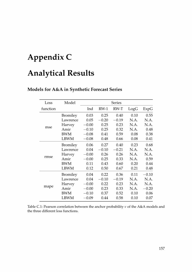
Appendix C
Analytical Results
Models for A&A in Synthetic Forecast Series
Loss Model Series
function Ind RW-1 RW-T LogG ExpG
mse
Bromiley 0.03 0.25 0.40 0.10 0.55Lawrence 0.05 −0.20 −0.19 N.A. N.A.Harvey −0.00 0.25 0.23 N.A. N.A.Amir −0.10 0.25 0.32 N.A. 0.48BWM −0.08 0.41 0.59 0.08 0.38LBWM −0.08 0.48 0.66 0.08 0.41
rmse
Bromiley 0.06 0.27 0.40 0.23 0.68Lawrence 0.04 −0.10 −0.21 N.A. N.A.Harvey −0.00 0.26 0.26 N.A. N.A.Amir −0.00 0.25 0.33 N.A. 0.59BWM 0.11 0.43 0.60 0.20 0.44LBWM 0.12 0.50 0.67 0.21 0.48
mape
Bromiley 0.04 0.22 0.36 0.11 −0.10Lawrence 0.04 −0.10 −0.19 N.A. N.A.Harvey −0.00 0.22 0.23 N.A. N.A.Amir −0.00 0.23 0.33 N.A. −0.20BWM −0.10 0.37 0.52 0.10 0.06LBWM −0.09 0.44 0.58 0.10 0.07
Table C.1: Pearson correlation between the anchor probability ν of the A&A models andthe three different loss functions.
157

158 Analytical Results
Series Model Bromiley Lawrence Harvey Amir BWM LBWM
Ind
Bromiley 1.00 −0.10 0.32 0.26 0.15 0.23Lawrence 1.00 −0.10 −0.00 0.09 0.10Harvey 1.00 0.83 0.01 0.03Amir 1.00 0.01 0.03BWM 1.00 0.90LBWM 1.00
RW-1
Bromiley 1.00 −0.20 0.36 0.31 0.30 0.35Lawrence 1.00 −0.30 −0.20 −0.10 −0.10Harvey 1.00 0.87 0.16 0.21Amir 1.00 0.15 0.20BWM 1.00 0.93LBWM 1.00
RW-T
Bromiley 1.00 0.08 −0.17 0.07 0.40 0.45Lawrence 1.00 −0.68 −0.55 −0.12 −0.12Harvey 1.00 0.80 0.13 0.15Amir 1.00 0.15 0.16BWM 1.00 0.93LBWM 1.00
LogG
Bromiley 1.00 N.A. N.A. N.A. 0.92 0.94Lawrence 1.00 N.A. N.A. N.A. N.A.Harvey 1.00 N.A. N.A. N.A.Amir 1.00 N.A. N.A.BWM 1.00 0.99LBWM 1.00
ExpG
Bromiley 1.00 N.A. N.A. 0.96 −0.10 −0.10Lawrence 1.00 N.A. N.A. N.A. N.A.Harvey 1.00 N.A. N.A. N.A.Amir 1.00 −0.20 −0.20BWM 1.00 0.96LBWM 1.00
Table C.2: Pearson correlation between the anchor probability ν of the A&A models.
References
Abarbanell, J. and R. Lehavy (2003). Biased Forecasts or Biased Earn-ings? The Role of Reported Earnings in Explaining Apparent Bias andOver/Underreaction in Analysts’ Earnings Forecasts. Journal of Accounting andEconomics 36(1), 105–146.
Almeida, H., M. Campello, and M. S. Weisbach (2004). The Cash Flow Sensitivityof Cash. Journal of Finance 59(4), 1777–1804.
Amir, E. and Y. Ganzach (1998). Overreaction and Underreaction in Analysts’Forecasts. Journal of Economic Behavior & Organization 37(3), 333–347.
Armstrong, J. S. and F. Collopy (1992). Error Measures for Generalizing aboutForecasting Methods: Empirical Comparisons. International Journal of Forecast-ing 8(1), 69–80.
Ashiya, M. (2003). Testing the Rationality of Japanese GDP Forecasts: The Signof Forecast Revision Matters. Journal of Economic Behavior & Organization 50(2),263–269.
Ashiya, M. (2006). Testing the Rationality of Forecast Revisions Made by the IMFand the OECD. Journal of Forecasting 25(1), 25–36.
Ball, R. and R. Watts (1972). Some Time Series Properties of Accounting Income.The Journal of Finance 27(3), 663–681.
Bartz-Beielstein, T., M. Chiarandini, L. Paquete, and M. Preuss (2010). Experimen-tal Methods for the Analysis of Optimization Algorithms. Springer.
Berinato, S. (2001). What Went Wrong at Cisco in 2001. CIO.com.http://cio.com/article/2441400/it-organization/what-went-wrong-at-cisco-in-2001.html.
Bessler, D. A. and J. A. Brandt (1992). An Analysis of Forecasts of Livestock Prices.Journal of Economic Behavior & Organization 18(2), 249–263.
159

160 References
Boiney, L. G., J. Kennedy, and P. Nye (1997). Instrumental Bias in MotivatedReasoning: More When More is Needed. Organizational Behavior and HumanDecision Processes 72(1), 1–24.
Brighton, H. and G. Gigerenzer (2015). The Bias Bias. Journal of Business Re-search 68(8), 1772–1784.
Bromiley, P. (1987). Do Forecasts Produced by Organizations Reflect Anchoringand Adjustment? Journal of Forecasting 6(3), 201–210.
Buehler, R. and D. Griffin (2003). Planning, Personality, and Prediction: The Roleof Future Focus in Optimistic Time Predictions. Organizational Behavior andHuman Decision Processes 92(1), 80–90.
Burgstahler, D. and I. Dichev (1997). Earnings Management to Avoid EarningsDecreases and Losses. Journal of Accounting and Economics 24(1), 99–126.
Burgstahler, D. and M. Eames (2006). Management of Earnings and Analysts’Forecasts to Achieve Zero and Small Positive Earnings Surprises. Journal ofBusiness Finance & Accounting 33(5–6), 633–652.
Chapman, P., J. Clinton, R. Kerber, T. Khabaza, T. Reinartz, C. Shearer, andR. Wirth (1999). CRISP-DM 1.0: Step-by-step data mining guide.
Clements, M. P. (1995). Rationality and the Role of Judgement in MacroeconomicForecasting. The Economic Journal 105(429), 410–420.
Clements, M. P., F. Joutz, and H. O. Stekler (2007). An Evaluation of the Fore-casts of the Federal Reserve: A Pooled Approach. Journal of Applied Economet-rics 22(1), 121–136.
Dalrymple, D. J. (1987). Sales Forecasting Practices: Results from a United StatesSurvey. International Journal of Forecasting 3(3-4), 379–391.
Dana, J. and R. M. Dawes (2004). The Superiority of Simple Alternatives to Re-gression for Social Science Predictions. Journal of Educational and BehavioralStatistics 29(3), 317–331.
Daniel, N. D., D. J. Denis, and L. Naveen (2008). Do Firms Manage Earnings toMeet Dividend Thresholds? Journal of Accounting and Economics 45(1), 2–26.
Davenport, T. H. and J. E. Short (2003). Information Technology and BusinessProcess Redesign. Operations Management: Critical Perspectives on Business andManagement 1, 97–123.

References 161
Dechow, P., W. Ge, and C. Schrand (2010). Understanding Earnings Quality: AReview of the Proxies, Their Determinants and Their Consequences. Journal ofAccounting and Economics 50(2), 344–401.
Dechow, P. M. (1994). Accounting Earnings and Cash Flows as Measures of FirmPerformance: The Role of Accounting Accruals. Journal of Accounting and Eco-nomics 18(1), 3–42.
DeFond, M. L. and M. Hung (2003). An Empirical Analysis of Analysts’ CashFlow Forecasts. Journal of Accounting and Economics 35(1), 73–100.
Degeorge, F., J. Patel, and R. Zeckhauser (1999). Earnings Management to ExceedThresholds. Journal of Business 72(1), 1–33.
Deschamps, B. and C. Ioannidis (2013). Can Rational Stubbornness Explain Fore-cast Biases? Journal of Economic Behavior & Organization 92, 141–151.
Dovern, J. and J. Weisser (2011). Accuracy, Unbiasedness and Efficiency of Pro-fessional Macroeconomic Forecasts: An Empirical Comparison for the G7. In-ternational Journal of Forecasting 27(2), 452–465.
Dowle, M., A. Srinivasan, J. Gorecki, T. Short, S. Lianoglou, and E. Antonyan(2015). data.table: Extension of ’data.frame’. Package version 1.9.6.
Easterwood, J. C. and S. R. Nutt (1999). Inefficiency in Analysts’ Earnings Fore-casts: Systematic Misreaction or Systematic Optimism? The Journal of Fi-nance 54(5), 1777–1797.
Fama, E. F. (1970). Efficient Capital Markets: A Review of Theory and EmpiricalWork. The Journal of Finance 25(2), 383–417.
Fildes, R., P. Goodwin, and M. Lawrence (2006, October). The Design Featuresof Forecasting Support Systems and Their Effectiveness. Decision Support Sys-tems 42(1), 351–361.
Fildes, R., P. Goodwin, M. Lawrence, and K. Nikolopoulos (2009). Effective Fore-casting and Judgmental Adjustments: An Empirical Evaluation and Strategiesfor Improvement in Supply-Chain Planning. International Journal of Forecast-ing 25(1), 3–23.
Fildes, R. and R. Hastings (1994). The Organization and Improvement of MarketForecasting. Journal of the Operational Research Society 45(1), 1–16.

162 References
Frankel, J. A. and K. Froot (1991). Chartists, Fundamentalists and the Demandfor Dollars. NBER Working Paper No. R1655.
Givoly, D. and J. Lakonishok (1979). The Information Content of Financial Ana-lysts’ Forecasts of Earnings: Some Evidence on Semi-Strong Inefficiency. Journalof Accounting and Economics 1(3), 165–185.
Goecke, H., W. J. Luhan, and M. W. Roos (2013). Rational Inattentiveness in aForecasting Experiment. Journal of Economic Behavior & Organization 94, 80–89.
Goodwin, P. (1996). Statistical Correction of Judgmental Point Forecasts and De-cisions. Omega 24(5), 551–559.
Gordon, L. A. and D. Miller (1976). A contingency framework for the designof accounting information systems. Accounting, Organizations and Society 1(1),59–69.
Graham, J. R. and C. R. Harvey (2001). The Theory and Practice of CorporateFinance: Evidence from the Field. Journal of Financial Economics 60(2), 187–243.
Guidry, F., A. J. Leone, and S. Rock (1999). Earnings-Based Bonus Plans andEarnings Management by Business-Unit Managers. Journal of Accounting andEconomics 26(1), 113–142.
Haigh, M. S. and J. A. List (2005). Do Professional Traders Exhibit Myopic LossAversion? An Experimental Analysis. The Journal of Finance 60(1), 523–534.
Han, J., J. Pei, and M. Kamber (2011). Data Mining: Concepts and Techniques. Else-vier.
Harvey, N., F. Bolger, and A. McClelland (1994). On the Nature of Expectations.British Journal of Psychology 85(2), 203–229.
Healy, P. M. (1985). The Effect of Bonus Schemes on Accounting Decisions. Journalof Accounting and Economics 7(1-3), 85–107.
Hogarth, R. M. and S. Makridakis (1981). Forecasting and Planning: An Evalua-tion. Management Science 27(2), 115 – 138.
Holthausen, R. W., D. F. Larcker, and R. G. Sloan (1995). Annual Bonus Schemesand the Manipulation of Earnings. Journal of Accounting and Economics 19(1),29–74.

References 163
Isiklar, G., K. Lahiri, and P. Loungani (2006). How Quickly do Forecasters In-corporate News? Evidence from Cross-Country Surveys. Journal of AppliedEconometrics 21(6), 703–725.
Jacob, J. and B. N. Jorgensen (2007). Earnings Management and Accounting In-come Aggregation. Journal of Accounting and Economics 43(2), 369–390.
Jacowitz, K. E. and D. Kahneman (1995). Measures of Anchoring in EstimationTasks. Personality and Social Psychology Bulletin 21(11), 1161–1166.
James, G., D. Witten, T. Hastie, and R. Tibshirani (2013). An Introduction to Statis-tical Learning, Volume 112. Springer.
John, T. A. (1993). Accounting Measures of Corporate Liquidity, Leverage, andCosts of Financial Distress. Financial Management 22(3), 91–100.
Kaplan, S. N. and R. S. Ruback (1995). The Valuation of Cash Flow Forecasts: AnEmpirical Analysis. The Journal of Finance 50(4), 1059–1093.
Kim, C., D. Mauer, and A. Sherman (1998). The Determinants of Corporate Liq-uidity: Theory and Evidence. Journal of Financial and Quantitative Analysis 33(3),335–359.
Kim, K. and D. A. Schroeder (1990). Analysts’ Use of Managerial Bonus Incen-tives in Forecasting Earnings. Journal of Accounting and Economics 13(1), 3–23.
Knöll, F. (2018). The Goal of Forecasting—Predictability of Cash Flow Revisionsin Corporate Finance. Working Paper in Preparation for the European Conferenceon Information Systems. Under Review.
Knöll, F., V. Dorner, and T. Setzer (2016). Relating Cash Flow Forecast Errorsto Revision Patterns. In Multikonferenz Wirtschaftsinformatik (MKWI) 2016: Pre-scriptive Analytics in IS, Volume 2, pp. 1217–1228. Universitätsverlag Ilmenau.
Knöll, F., V. Dorner, and T. Setzer (2018). When Inefficiency Seems Beneficial—Organizational Issues versus Cognitive Biases in Corporate Cash Flow Fore-casting. Working Paper in Journal Preparation.
Knöll, F. and J. Huber (2018). Forecast Correction in Judgmental Cash Flow Re-visions. Working Paper in Preparation for the International Conference on ExploringService Science. Under Review.

164 References
Knöll, F. and D. Roßbach (2018a). Anchor and Adjustment Detection on Empir-ical Forecast Series. In Multikonferenz Wirtschaftsinformatik (MKWI) 2018: DataAnalytical Processes in IS, Volume 1, pp. 257–268. Leuphana Universität Lüneb-urg.
Knöll, F. and D. Roßbach (2018b). The Anchor and Adjustment Bandwidthmodel:Exploring Cognitive Biases in Simulated Forecast Series. In Proceedings of the51st Hawaii International Conference on System Sciences (HICSS), 2018, pp. 1533–1542.
Knöll, F., T. Setzer, and K. Laubis (2018). On Predictability of Revisioning inCorporate Cash Flow Forecasting. In Proceedings of the 51st Hawaii InternationalConference on System Sciences (HICSS), 2018, pp. 1583–1589.
Knöll, F. and K. Shapoval (2018). Forecast Correction Using Organizational Debi-asing in Corporate Cash Flow Revisioning. Working Paper in Preparation for theInternational Conference on Exploring Service Science. Under Review.
Knöll, F. and V. Simko (2017). Organizational Information improves Forecast Effi-ciency of Correction Techniques. In Proceedings of the 17th Conference on Informa-tion Technologies – Applications and Theory (ITAT), Computational Intelligence andData Mining (WCIDM 2017), Volume 1885, pp. 86–92.
Kudla, R. J. (1976). Elements of Effective Corporate Planning. Long Range Plan-ning 9(4), 82–93.
Lawrence, M., P. Goodwin, M. O’Connor, and D. Önkal (2006). Judgmental Fore-casting: A Review of Progress Over the Last 25 Years. International Journal ofForecasting 22, 493–618.
Lawrence, M. and S. Makridakis (1989). Factors Affecting Judgmental Forecastsand Confidence Intervals. Organizational Behavior and Human Decision Pro-cesses 43(2), 172–187.
Lawrence, M. and M. O’Connor (1992). Exploring Judgemental Forecasting. In-ternational Journal of Forecasting 8(1), 15–26.
Lawrence, M. and M. O’Connor (1993). Scale, Randomness and the Calibration ofJudgmental Confidence Intervals. Organizational Behavior and Human DecisionProcesses 56, 441–458.
Lawrence, M. and M. O’Connor (2000). Sales Forecasting Updates: How Goodare They in Practice? International Journal of Forecasting 16(3), 369–382.

References 165
Leitner, J. and U. Leopold-Wildburger (2011). Experiments on Forecasting Behav-ior with Several Sources of Information – A Review of the Literature. EuropeanJournal of Operational Research 213(3), 459–469.
Lim, J. S. and M. O’Connor (1995). Judgemental Adjustment of Initial Forecasts:Its Effectiveness and Biases. Journal of Behavioral Decision Making 8(3), 149–168.
Lim, J. S. and M. O’Connor (1996). Judgmental Forecasting with Time Series andCausal Information. International Journal of Forecasting 12(1), 139–153.
Lim, S. S. and H. Wang (2007). The Effect of Financial Hedging on the Incentivesfor Corporate Diversification: The Role of Stakeholder Firm-Specific Invest-ments. Journal of Economic Behavior & Organization 62(4), 640–656.
Mannila, H. (1996). Data mining: machine learning, statistics, and databases.In Proceedings of the Eighth International Conference on Scientific and StatisticalDatabase Systems, pp. 2–9. IEEE.
Marr, B. (2012). Key Performance Indicators (KPI): The 75 Measures Every ManagerNeeds to Know. Pearson UK.
Martin, J. (2012). Quality Assurance in Corporate Financial Planning – A Process-and Data-Driven Perspective. Ph. D. thesis, Karlsruhe, Karlsruher Institut fürTechnologie (KIT), Dissertation, 2012.
Martin, J. D. and G. E. Morgan (1988). Financial Planning Where the Firm’s De-mand for Funds is Nonstationary and Stochastic. Management Science 34(9),1054–1066.
Mathews, B. P. and A. Diamantopoulous (1990). Judgemental Revision of SalesForecasts: Effectiveness of Forecast Selection. Journal of Forecasting 9(4), 407–415.
McCarthy, T. M., D. F. Davis, S. L. Golicic, and J. T. Mentzer (2006). The Evolutionof Sales Forecasting Management: A 20-Year Longitudinal Study of ForecastingPractices. Journal of Forecasting 25(5), 303.
McNees, S. K. (1975). An Evaluation of Economic Forecasts. New England Eco-nomic Review 16, 3–39.
McNees, S. K. (1990). The Role of Judgment in Macroeconomic Forecasting Ac-curacy. International Journal of Forecasting 6(3), 287–299.
166 References
Mendoza, M. and E. de Alba (2006). Forecasting an Accumulated Series Based onPartial Accumulation II: A new Bayesian Method for Short Series with StableSeasonal Patterns. International Journal of Forecasting 22(4), 781–798.
Mentzer, J. T. and J. E. Cox (1984). Familiarity, Application, and Performance ofSales Forecasting Techniques. Journal of Forecasting 3(1), 27–36.
Meub, L. and T. Proeger (2016). Can Anchoring Explain Biased Forecasts? Exper-imental Evidence. Journal of Behavioral and Experimental Finance 12, 1–13.
Nikolopoulos, K., M. Lawrence, P. Goodwin, and R. Fildes (2005). On the ac-curacy of judgmental interventions on forecasting support systems. WorkingPaper.
Nordhaus, W. D. (1987). Forecasting Efficiency: Concepts and Applications. TheReview of Economics and Statistics 69(4), 667–674.
Northcraft, G. B. and M. A. Neale (1987). Experts, Amateurs, and Real Estate: AnAnchoring-and-Adjustment Perspective on Property Pricing Decisions. Orga-nizational Behavior and Human Decision Processes 39(1), 84–97.
Noval, L. J. (2016). On the Misguided Pursuit of Happiness and Ethical DecisionMaking: The Roles of Focalism and the Impact Bias in Unethical and SelfishBehavior. Organizational Behavior and Human Decision Processes 133, 1–16.
Penman, S. H. (1980). An Empirical Investigation of the Voluntary Disclosure ofCorporate Earnings Forecasts. Journal of Accounting Research 18(1), 132–160.
Petrovits, C. M. (2006). Corporate-Sponsored Foundations and Earnings Man-agement. Journal of Accounting and Economics 41(3), 335–362.
Phillips, L. D. (1984). A Theory of Requisite Decision Models. Acta Psycholog-ica 56(1), 29–48.
R Core Team (2013). R: A Language and Environment for Statistical Computing. Vi-enna, Austria: R Foundation for Statistical Computing.
Roychowdhury, S. (2006). Earnings Management Through Real Activities Manip-ulation. Journal of Accounting and Economics 42(3), 335–370.
Sanders, N. R. and K. B. Manrodt (2003). The Efficacy of Using Judgmental VersusQuantitative Forecasting Methods in Practice. Omega 31(6), 511–522.

References 167
Sanders, N. R. and L. P. Ritzman (1995). Bringing Judgment into CombinationForecasts. Journal of Operations Management 13(4), 311–321.
Schweitzer, M. E., L. Ordóñez, and B. Douma (2004). Goal Setting as a Motivatorof Unethical Behavior. Academy of Management Journal 47(3), 422–432.
Shugan, S. M. and D. Mitra (2009, January). Metrics — When and Why Nonaver-aging Statistics Work. Management Science 55(1), 4–15.
Stulz, R. M. (1990). Managerial Discretion and Optimal Financing Policies. Journalof Financial Economics 26(1), 3–27.
Stulz, R. M. (1996). Rethinking Risk Management. Journal of Applied CorporateFinance 9(3), 8–25.
Switzer, F. S. and J. A. Sniezek (1991). Judgment Processes in Motivation: Anchor-ing and Adjustment Effects on Judgment and Behavior. Organizational Behaviorand Human Decision Processes 49(2), 208–229.
Syntetos, A. A., K. Nikolopoulos, J. E. Boylan, R. Fildes, and P. Goodwin (2009).The Effects of Integrating Management Judgement into Intermittent DemandForecasts. International Journal of Production Economics 118(1), 72–81.
Timmermann, A. and C. W. Granger (2004). Efficient Market Hypothesis andForecasting. International Journal of Forecasting 20(1), 15–27.
Tversky, A. and D. Kahneman (1975). Judgment Under Uncertainty: Heuris-tics and Biases. In Utility, Probability, and Human Decision Making, pp. 141–162.Springer.
Wansink, B., R. J. Kent, and S. J. Hoch (1998). An Anchoring and AdjustmentModel of Purchase Quantity Decisions. Journal of Marketing Research 35(1), 71–81.
Wei, T. and V. Simko (2016). corrplot: Visualization of a Correlation Matrix. Packageversion 0.77.
Wickham, H., W. Chang, and RStudio (2016). ggplot2: Create Elegant Data Visuali-sations Using the Grammar of Graphics. Package version 2.1.0.
Working, H. (1934). A Random-Difference Series for Use in the Analysis of TimeSeries. Journal of the American Statistical Association 29(185), 11–24.
Yelland, P. M. (2006). Stable Seasonal Pattern Models for Forecast Revision: AComparative Study. International Journal of Forecasting 22(4), 799–818.
