BIFURCATION BOUNDARIES IN ECONOMIC MODELS

JACQUES K NGOIE

UN Project Link

October 24, 2012

1

OUTLINE

Contributions and motivation of the study

Literature review

Definitions and Descriptions of Bifurcation boundaries

Empirical measurement techniques

Solution framework

Results and Conclusion

2

KEY CONTRIBUTIONS TO THE LITERATURE

Expand on bifurcation analysis of economic models

Provide empirical assessment techniques of bifurcation

boundaries in economic models

Provide technical ways to address the issue in economic

modeling

3

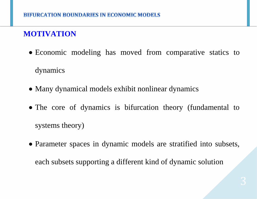
MOTIVATION

Economic modeling has moved from comparative statics to

dynamics

Many dynamical models exhibit nonlinear dynamics

The core of dynamics is bifurcation theory (fundamental to

systems theory)

Parameter spaces in dynamic models are stratified into subsets,

each subsets supporting a different kind of dynamic solution

4

Dynamic econometrics inference is produced from simulations

with parameters set only at point estimates instead of various

settings within the confidence region

Bifurcation boundaries damage several qualitative properties of

dynamic models

Stratification of confidence region into bifurcated subsets

seriously damages robustness of dynamic inference

5

To know whether the confidence region is crossed by bifurcation

boundaries, one needs to locate those boundaries

The uncertainty surrounding parameters leads to more

uncertainty about bifurcation boundaries linked to the par. space

6

LITERATURE REVIEW

First study on bifurcation boundaries was conducted by Poincare

(1885, 1892) for two-dimensional vector fields

Andronov (1929) formulated the first theorem on Hopf bifur. and

developed important tools for analysing nonlinear dynamical

systems (also for two-dimensional vect. fields)

Later on, in 1942, Hopf developed the most famous general

theorem on the existence of Hopf bifurcation – generalized to n

dimensional vector fields

7

Studies such as Torre (1977) for Keynesian systems and

Benhabib et al (1979) for multi-sectoral neoclassical optimal

growth models were among the first one to find Hopf bifurcation

boundaries in economic models

Later on, bifurcation boundaries were found in overlapping

generation models; see Benhabib et al (1982, 1991), Aiyagari

(1989), etc

In 1985, Grandmont expanded findings – par. space of even the

simplest classical general-equilibrium models are stratified into

bifurcation regions

8

More recent studies finding bifurcation boundaries in

econometric models such a Bergstrom continuous-time model,

the Leeper & Sims Euler-equations model, etc., include Barnett

and He (1999, 2001, 2002, 2004, 2006, 2008,2011)

Also, Barnett et al have expanded on the work of Grandmont

bringing policy relevance to his findings; see Barnett et al (2004,

2005),

Barnett and Duzhak (2008,2009) have investigated bifurcation

boundaries within the more recent class of New Keynesian

models

9

DEFINITIONS AND DESCRIPTIONS

Bifurcation refers to changes in qualitative features of solution

dynamics as parameter values change

When the system has no bifurcations boundaries, only changes in

quantitative features of dynamic solutions are observed

Bifurcation boundaries bring changes in qualitative features of

dynamics solutions such as monotonic convergence to damped

convergence to a steady state

10

Close to bifurcation boundaries, quantitative features of the

system become more sensitive to parameter changes

The use of parameter changes to assess the impact of policy

shifts using the model might lead to unreliable results

11

EXAMPLE

Let a continuous dynamic system (Barnett et al. 2008, Banerjee et al

2012)

)(xfx

, nx and 0x an equilibrium of the system

M: the Jacobian matrix dx

df evaluated at 0x

Let the numbers of eigenvalues of A

with negative real: n

with zero real: 0n

with positive real: n

12

Definition 1

We have an hyperbolic equilibrium when 0n .

It means no eigenvalues on the imaginary axis or unit circle.

Or, let the following two dynamical systems

),( xfx

, nx ,

m (1)

),( ygy

, ny ,

m (2)

13

Definition 2

We can say that (1) is topologically equivalent to (2) if

- there is existence of a homeomorphism of the parameter space

mmp : , )( p

- there is a parameter-dependent homeomorphism of the phase

space nnh : , )(xhy which maps the system’s orbits at

parameter values )( p while preserving the time direction

14

Definition 3

Presence of topologically non-equivalent phase portrait under

variation of parameters is called bifurcation.

At the non-hyperbolic points, sufficiently small perturbations of

parameters lead to changes in structural stability.

15

Definition 4

A transcritical bifurcation occurs when a system has non-hyperbolic

equilibrium with a geometrically simple zero eigenvalue at the

bifurcation point with additional transversality conditions.

16

Fig. 1 – Portrait phase of saddle-node bifurcation

17

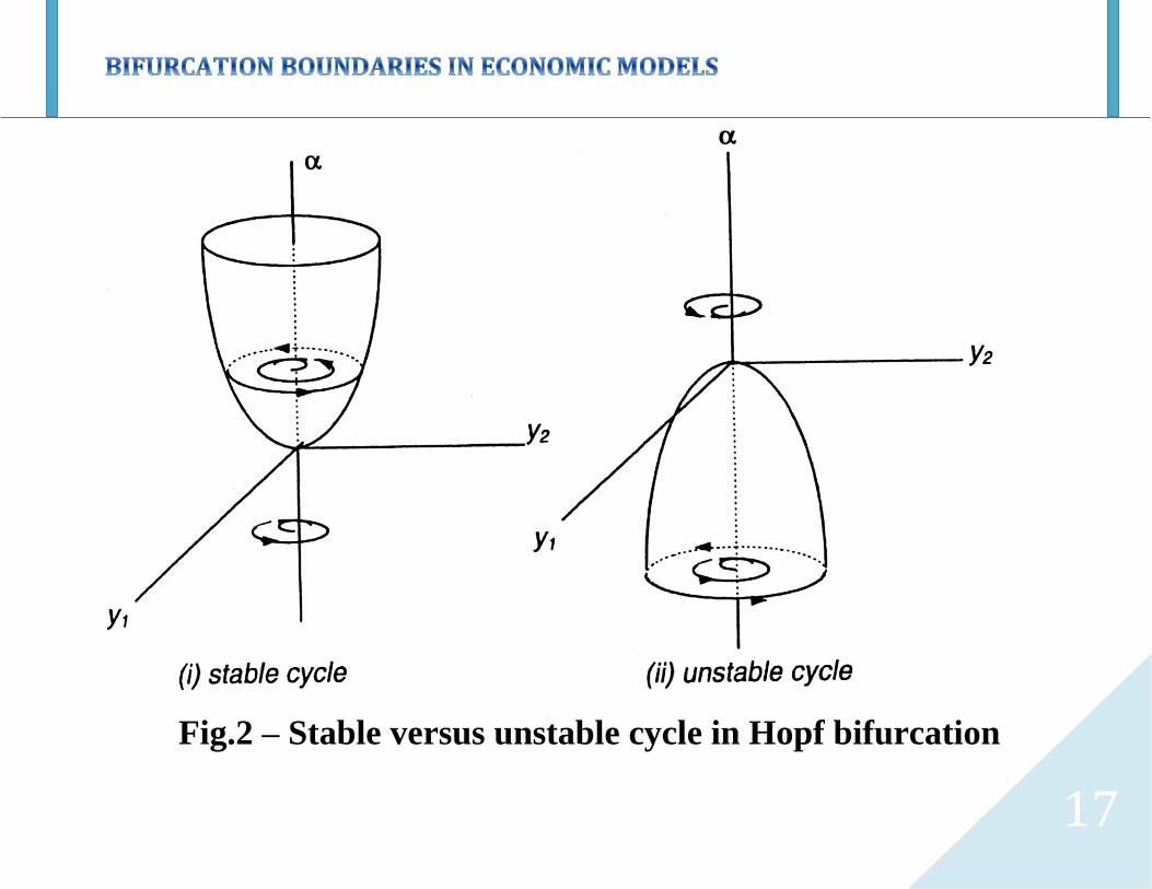
Fig.2 – Stable versus unstable cycle in Hopf bifurcation

18

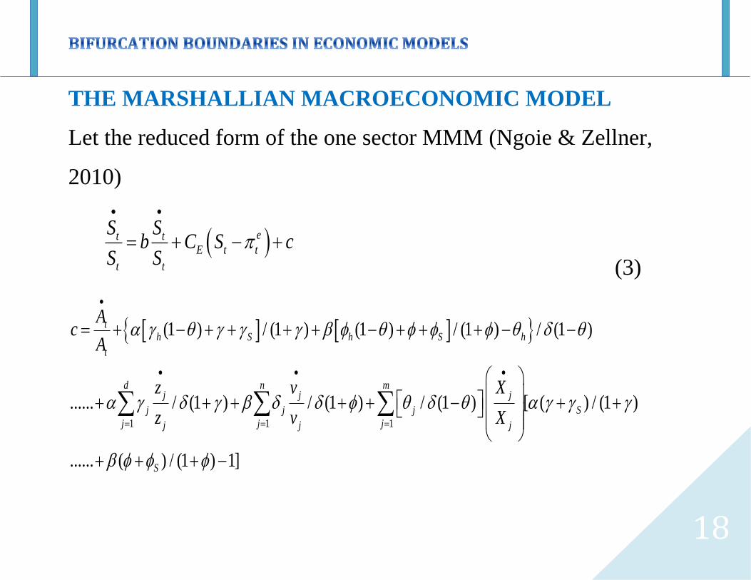
THE MARSHALLIAN MACROECONOMIC MODEL

Let the reduced form of the one sector MMM (Ngoie & Zellner,

2010)

et t

E t t

t t

S Sb C S c

S S

(3)

1 1 1

(1 ) / (1 ) (1 ) / (1 ) / (1 )

...... / (1 ) / (1 ) / (1 ) [ ( ) / (1 )

...... ( ) / (1 ) 1]

th S h S h

t

d n mj j j

j j j S

j j jj j j

S

Ac

A

z v X

z v X

19

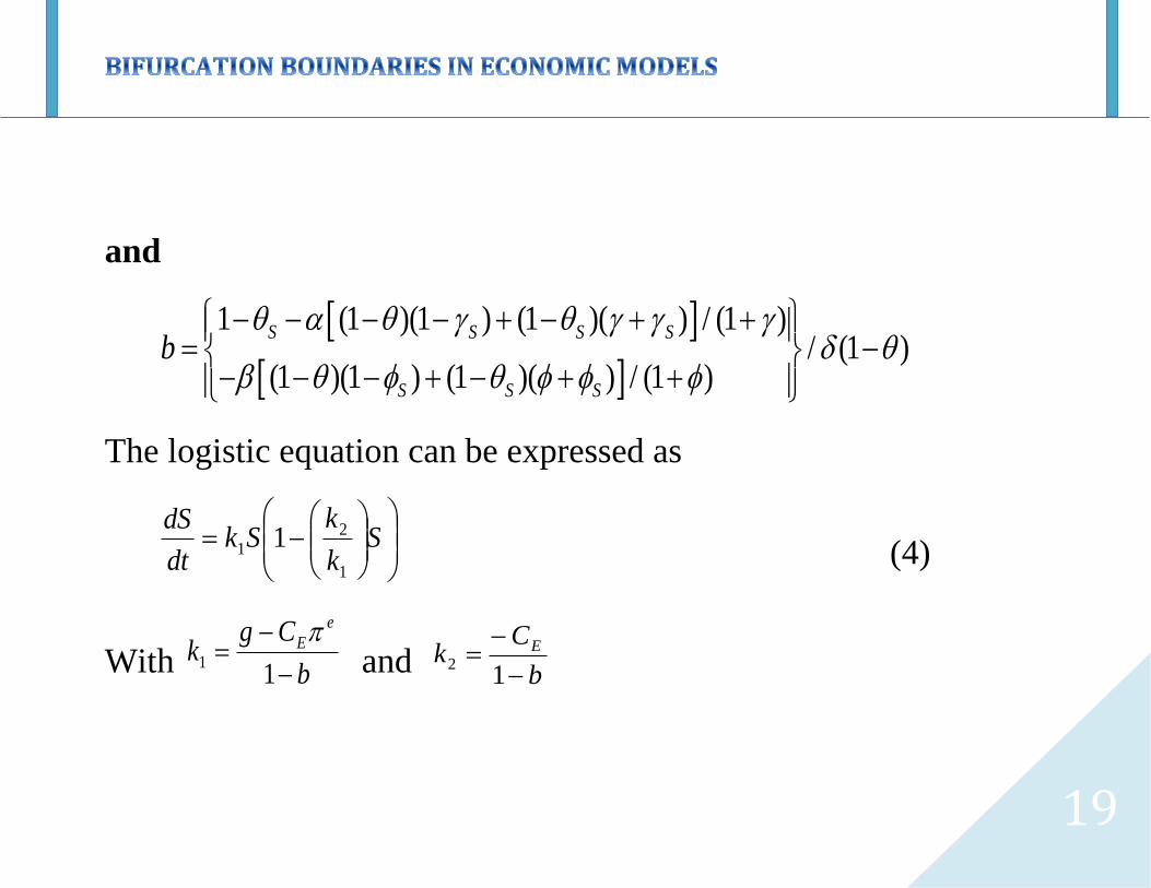
and

1 (1 )(1 ) (1 )( ) / (1 )/ (1 )

(1 )(1 ) (1 )( ) / (1 )

S S S S

S S S

b

The logistic equation can be expressed as

S

k

kSk

dt

dS

1

21 1

(4)

With b

Cgk

e

E

11

and b

Ck E

12

20

(4) has two equilibrium values 0S and 2

1

k

kS

For constant parameters there are no cyclical movements

For discrete lags there is mixed differential-difference equation

that can produce cyclical solutions

21

Fig.3 – Stability of equilibrium solutions

22

SOLUTION FRAMEWORK

MODELS WITH ANALYTICAL SOLUTIONS

1. Construct an acceptance region

Optimize and obtain the model’s solution either from its reduced

form or any other form

Construct an A-R (Accept Reject) algorithm to reconstruct an

acceptance region, i.e. a region without bifurcation boundaries –

A-R algorithm will restrict the acceptance sample to be iid

To remove that restriction, I also construct a M-H (Metropolis

Hastings) algorithm

23

The Accept-Reject algorithm

The algorithm is used to generate the required parameter space

only with draws that pass the set conditions

This algorithm allows to generate a candidate space from

virtually any type of distribution

Using the known functional form of the density of interest f (the

target density) as well as the conditions of acceptance for the

parameters space

From f, I use a simpler density g (the candidate density) to

generate rv that satisfy my parameter space

24

Constraints

Compatible support for both densities f and g, i.e. g(x)>0 when

f(x)>0 and vice versa

I use a constant C such as

for all x

g(x) contains only draws that satisfy the ‘no bifurcation

boundaries’ condition

25

To illustrate

X can be simulated as follows:

1. I generate and independently, I also generate

2. If

, then I set X=Y

3. Should the inequality not being satisfied, the algorithm discards

Y and U and start all over again

26

Algorithm representation

1. Form g with draws that match the conditions

2. Generate , ;

3. Accept X = Y if

4. Return to 2 otherwise

27

Proof that the method works

It can be proven that the cdf of the accepted sample,

| { }

is exactly the same as the cdf of X.

( |

{ })

{ }

{ }

28

∫ ∫

{ }

∫ ∫

{ }

∫ [

{ }]

∫ [

{ }]

29

∫

∫

,

Which proves that the cdf of the accepted sample is the same as the

cdf of X.

30

The impact of bifurcation boundaries can therefore be assessed

looking at the acceptance probability

The higher the probability, the less concerned we should be

about bifurcation boundaries

The A-R algorithm helps derive a uniform distribution

31

The Metropolis-Hastings Algorithm

M-H algorithm is far more sophisticated than the A-R algorithm

as it removes the iid restriction on the candidate sample

Yt are generated independently but the resulting sample is not iid

Probability of acceptance of Yt depends on a Markov chain X(t)

The M-H is a straightforward generalization of the A-R method

The M-H involves repeated occurences of the sample value since

rejection of Yt leads to repetition of X(t)

at time t+1

32

A-R acceptance steps require the calculation of the upper bound

.

This is not required by the M-H algorithm

The M-H requires very little knowledge about f

33

HOW DOES IT WORK?

Given a target density f, I build a markov kernel K with

stationary distribution f and then generate a markov chain using

this kernel.

The limiting distribution of )( )(tX is f and integrals can be

approximated according to the Ergodic Theorem

The key issue here is therefore to construct a kernel K that is

associated with an arbitrary density f.

34

Given the target density f, the kernel is associated with working

conditional density )( xyq that is easy to simulate.

Also, q can be almost arbitrary in that the only theoretical

requirements are that the ratio )(

)(

xyq

yf

is known up to a constant

independent x and that )( xq has enough dispersion to lead to an

exploration of the entire support of f.

For every given q, I can construct a Metropolis_Hastings kernel such

that f is stationary distribution.

35

The algorithm

The M-H algorithm associated with the objective density f and the

conditional density q produces a markov chain through the following

transition kernel:

1.Generate )(~ )(t

t xyqY

2.Take

),,(1..............

),,(.....................)()(

)(

)1(

t

tt

t

t

tt

Yxyprobabilitwithx

YxyprobabilitwithYX

where

1,(

)(

)(

)(min),(

xyq

yxq

xf

yfyx

36

2. BAYESIAN ESTIMATION USING PRIOR

INFORMATION

I construct an informative prior (conjugate in case of the A-R

algorithm) using information obtained from the algorithms

In the case of M-H, the prior can be improper

I associate the problem to Bernoulli trial where the success is

attributed to draws within the acceptance region and the failure

outside of the region

37

I make use of the A-R or M-H algorithm to build an informative

beta prior using Bernoulli distribution with know probability of

success

Compute the posterior odd between the two models: (1) a model

using the new prior (the one accounting for bifurcation

boundaries); and (2) a model using a similar prior that does not

account for bifurcation boundaries

38

The usual conjugate prior associated to the Bernoulli distribution

is the Beta prior obtained from a beta distribution.

Considering an observation x such as

,

From this, we can extract a family of conjugate priors as

{

}

,

with the hyperparameters

39

The posterior is as follows:

| {

}

,

The problem here is that difficulty of dealing with gamma

functions make it impossible to simulate directly from | .

It is required to make use of a substitute distribution and

integrate using Monte Carlo methods.

40

3. CASE OF MIXTURE REPRESENTATIONS

The mixture distribution can be represented as follows.

∫ |

with the auxiliary continuous space and g and p, two standard

distributions.

In order to generate a rv X using such a representation, I first

generate a variable Y from the mixing distribution and then generate

X from the selected conditional distribution.

For and | , then in continuous space

41

RESULTS

Table 1 - Acceptance rates

Algorithm Acceptance rate (%) Kolmogorov Sm. test

A-R 68 0.0203

M-H 71 0.0301

42

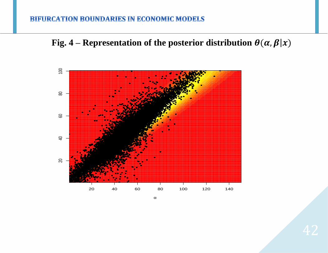
Fig. 4 – Representation of the posterior distribution |

20 40 60 80 100 120 140

2040

6080

100

a

43

Posterior odds between models

Model 1 (M1) – Model that ignores bifurcation boundaries (no

distinction between acceptance and rejection in the prior)

Model 2 (M2) – Model accounting for bifurcation boundaries

(information about acceptance region included in the prior)

|

|

A posterior odd of 0.24 (1:4.2) strongly support

consideration of bifurcation boundaries.

44

Fig. 5 – Histogram of 10^6 rv generated from the mixture

representation along the probability function

x

Den

sity

0 10 20 30 40 50 60 70

0.00

0.01

0.02

0.03

0.04

0.05

0.06

45

CONCLUSION

Bifurcation boundaries remain a treat to policy guidance

provided by dynamic models and reduce the confidence region

This study unveils tools useful to redefine the confidence region

in the presence of bifurcation boundaries

This research provides a solution framework allowing Bayesian

inferences to provide estimates that control for bifurcation

boundaries