big data management for periodic wireless sensor networks
TRANSCRIPT

HAL Id: tel-01228515https://tel.archives-ouvertes.fr/tel-01228515
Submitted on 13 Nov 2015
HAL is a multi-disciplinary open accessarchive for the deposit and dissemination of sci-entific research documents, whether they are pub-lished or not. The documents may come fromteaching and research institutions in France orabroad, or from public or private research centers.
L’archive ouverte pluridisciplinaire HAL, estdestinée au dépôt et à la diffusion de documentsscientifiques de niveau recherche, publiés ou non,émanant des établissements d’enseignement et derecherche français ou étrangers, des laboratoirespublics ou privés.
Big data management for periodic wireless sensornetworks
Maguy Medlej
To cite this version:Maguy Medlej. Big data management for periodic wireless sensor networks. Data Structures and Al-gorithms [cs.DS]. Université de Franche-Comté, 2014. English. �NNT : 2014BESA2029�. �tel-01228515�

Copyright
By
Maguy Medlej
2014

Big Data Management in
Periodic Wireless Sensor Networks
Maguy Medlej
By
Thèse soutenue le 30 juin 2014

The Thesis Committee for University of Franche-Comté
Certifies that this is the approved version of the following thesis:
Big Data Management in Periodic Wireless Sensor Networks
THESIS COMMITTEE:
Pr. Salima Benbernou, University of Paris Descartes, Reviewer
Pr. Hamamache Kheddouci, University of Claude Bernard - Lyon 1, Reviewer
Pr. Congduc Pham, University of Pau, Examinator
Pr. Olga Kouchnarenko, University of Franche-Comté, Examinator
Pr. Jacques Bahi, University of Franche-Comté, Ph.D Director
Dr. Abdallah Makhoul, University of Franche-Comté, Supervisor

Big Data Management in Periodic Wireless Sensor Networks
by
Maguy Medlej
Thesis
Presented to
the University of Franche Comté
in Partial Fulfillment
of the Requirements
for the Degree of
PHD
The University of Franche Comté
June, 30 2014

Dedication
This thesis work is foremost dedicated to my husband, Maroun, who has been a
constant source of support and encouragement during the challenges and the hardships of
this journey. Maroun, your words of encouragement and endorsement for tenacity ring in
my ears. I am truly thankful for having you in my life.
I would like to extend my dedication to Dr. Abdallah Makhoul who supported me
throughout my journey. I will always appreciate his tireless efforts in scaling up my
technical skills, and the countless hours of proofreading he spent.
I dedicate this work as well to my baby girl Skye whom innocent smile gave me
the strength to overcome the hardest moments I endured, especially during my last year
of this thesis. Baby, you have been my best cheerleader.
A special feeling of gratitude to my mom who supported me in my determination
to find and realise my potential. Mom, thank you for your continuous support throughout
my life.
Last but most certainly not least, this thesis is dedicated to the loving memory of
my father. Dad, Thank you for being there and doing your best with so little you had.
You have been my silent inspiration to thrive. Till we meet again, I will always be your
little girl.

vi
Acknowledgements
The long journey of my doctoral study has ended. It is with great delight that I
acknowledge my debts to those who have greatly contributed to the success of this
thesis.
Foremost, I would like to express my sincere gratitude to both my advisors
Prof. Jacques Bahi and Dr. Abdallah Makhoul for their continuous support for my
Ph.D study and research, their patience, motivation, enthusiasm, and immense
knowledge. Their tireless guidance has helped me immensely in researching and
writing this thesis. I could not have imagined having better advisors and mentors. I am
also particularly grateful to Dr. Abdallah Makhoul for enlightening me the first glance
of research.
Besides my advisors, I would like to express my gratitude to Prof. Salima
Benbernou and Prof. Hamamache Kheddouci for accepting to review my manuscript
and for their insightful and appreciated comments. I would like to thank also Prof.
Congduc Pham and Prof. Olga Kouchnarenko for accepting to participate to my thesis
committee.
This work would have never been possible without the support, persistence
and endurance of my husband Maroun Khoury.
Last but not the least, I would like to thank God for his blessings, his grace,
wisdom, favor, faithfulness and protection especially that he blessed me with a
wonderful girl last year.

vii
Abstract
Big Data Management in Wireless Sensor Networks
Maguy Medlej
The University of Franche Comté, 2014
Supervisors: Jacques Bahi, Abdallah Makhoul
Tides of readings are generated by small sensor nodes which constitute a
wireless sensor networks (wsn) providing powerful silos of information that aims to
leverage business profitability and enable environmental benefits. The promising
results of wsn deployment in medical, commercial, industrial and military
applications coupled with the acute need for real time decision making and periodic
data collection especially in remote or menacing environments intrigued data
consortiums and network communities to invest heavily in this field. Researches
focused mainly on the limitations imposed by wsn in terms of energy, computing and
communication capacity. This thesis proposes novel big data management techniques
for periodic sensor networks embracing the limitations imposed by wsn and the nature
of sensor data.
First, we proposed an adaptive sampling approach for periodic data collection.
The main idea behind this approach is allowing each sensor node to adapt its sampling
rates to the physical changing dynamics. In this way, over-sampling can be minimized
and power efficiency of the overall network system can be improved dramatically.
We present an efficient adaptive sampling approach based on the dependence of
conditional variance of measurements over time. Then, we propose a multiple level
activity model that uses behavioral functions modeled by modified Bezier curves to
define application classes and allow for sampling adaptive rate.
Then we shift gears to address the periodic data aggregation on the level of
sensor node data as a preprocessing phase for an efficient and scalable data mining.
For this purpose, we introduced two tree-based bi-level periodic data aggregation

viii
techniques for periodic sensor networks. The first one look on a periodic basis at each
data measured at the first tier then, clean it periodically while conserving the number
of occurrences of each measure captured. Lastly, data aggregation is performed
between groups of nodes on the level of the aggregator while preserving the quality of
the information. The second one proposes a new data aggregation approach aiming to
identify near duplicate nodes that generate similar sets of collected data in periodic
applications. We suggest the prefix filtering approach that avoids computing
similarity values for all possible pairs of sets. We define a new filtering technique
based on the quality of information.
Last but not least, we propose a new data mining method depending on the
existing K-means clustering algorithm to mine the aggregated cleaned data and
overcome the high computational cost imposed by data mining techniques as well as
sensor networks limitations in terms of energy and power. We developed a new
multilevel optimized version of « k-means » based on prefix filtering technique. K-
means optimization technique in terms of comparison and number of iterations is
applied by exploiting prefix subsets of data. The main idea of this technique is to
optimize the clustering of observations generated by sensor networks into groups of
related readings without any prior knowledge of the relationships between the
prefixes sets.
All the proposed approaches for data management in periodic sensor networks
are validated through simulation results based on real data generated by periodic
wireless sensor network. These results show the importance of the suggested approach
in terms of energy optimization, performance and data quality needed for decision
making, analysis and business benefits.

ix
Résumé
Gestion de données volumineuses dans les réseaux de capteurs
périodiques
Maguy Medlej
Université de Franche Comté, 2014
Encadrants: Prof. Jacques Bahi, Dr. Abdallah Makhoul
Durant la dernière décennie, sont apparus les réseaux de capteurs sans fils. Ces
réseaux facilitent le suivi et le contrôle à distance de l’environnement physique avec
une meilleure précision. Ils peuvent avoir de très diverses applications
(environnementales, militaires, médicales, etc). Notons qu’un réseau de capteurs est
constitué d’un grand nombre d’unités appelées noeuds capteurs. Chaque noeud est
composé principalement d’un ou plusieurs capteurs, d’une unité de traitement et d’un
module de communication.
La diversité d’application d’un réseau de capteurs fait que cette nouvelle
technologie soit orientée application. Parmi les applications les plus répandues est la
sureveillance environementale. Les capteurs environnementaux sont des composants
électroniques qui peuvent être utilisés pour mesurer/capter des paramètres de
l’environnement comme la température, l’humidité, la pression atmosphérique, la
concentration d’un gaz particulier dans l’air, etc. Un réseau de capteurs
environnemental permet de très diverses applications comme, le suivi de la qualité des
eaux souterraines, la surveillance de la pollution dans une ville, les systèmes
d’arrosage, la surveillance des glaciers montagneux, etc.
La collecte des données auprès des réseaux de capteurs environnementaux
peut être réalisée à la demande par un dialogue bi-directionnel entre les noeuds et la
station de base, ou bien sans demande. Cependant, dans la majorité des cas le modèle

x
de collecte de données adopté est le modèle d’échantillonnage périodique. Ce modèle
est caractérisé par l’acquisition de données par les noeuds capteurs à distance et sa
transmission à la station de base d’une manière périodique. Nous appelons réseau de
capteur périodique, un réseau de capteur adoptant le modèle d’échantillonnage
périodique pour la collecte de données.
Les réseaux de capteurs périodiques, tout comme les réseaux de capteurs
traditionnels présentent de nombreuses contraintes, telles que la bande passante, la
puissance de calcul, la mémoire disponible ainsi que la consommation d’énergie.
Cependant, un défi majeur dans les réseaux périodiques est la gestion de données. En
effet, comme chaque noeud est une source de données, et comme il peut être équipé
d’un ou de plusieurs capteurs, de nombreurses données seront recueillies. Cependant,
l'analyse des flux de données pour obtenir des informations et prendre des décisions
appropriées, est l'un des challenges de conception pour les réseaux de capteurs
périodiques. La gestion des données n'est pas une tâche facile, en particulier pour les
réseaux de capteurs d'énergie limitée et ce qui constiue l’objectif principal de cette
thèse.
Dans cette thèse, notre travail principal consiste à réduire la grande masse de
données générée par les réseaux de capteurs périodiques tout en conservant son
intégrité. Nous avons proposé des modèles de gestion de données volumineuses de la
collecte de données à la prise de décision. En effet, nous avons conçu un modèle
permettant à chaque noeud d’adapter son taux d’échantillonnage à l’évolution
dynamique de l’environnement. Par ce modèle on réduit le sur-échantillonnage et par
conséquent on réduit la quantité d’énergie consommée. Une deuxième technique
permettant la réduction de taille de données est l’agrégation. En effet, les données
produites par les capteurs voisins sont très corrélées spatialement et temporellement.
Ceci peut engendrer la réception par l’utilisateur final d'informations redondantes.
Réduire la quantité de données redondantes transmises par les noeuds permet de
réduire la consommation d'énergie dans le système et prépare les données pour la
prise de décision. Ensuite, un modèle de fouille de données est proposé et adapté à
notre cas.

xi
Ces travaux sont présentés dans cette thèse en 6 chapitres.
Dans le chapitre II, nous commençons par une présentation générale des
réseaux de capteurs périodiques tout en mettant en valeur leurs applications et leur
caractérisques. Ensuite, les differents défits de ces réseaux en plus des défis imposés
par la gestion des données volumineuse générées par les reseaux de capteurs
périodiques sont présentés tels que la collecte, la latence and l’integrité des données.
Un premier objectif a consisté à réduire cette masse de données tout en
conservant son intégrité. Pour cela, le problème de la collecte de données dans les
réseaux de capteurs périodiques est abordé dans le chapitre III. Nous avons conçu un
modèle permettant à chaque nœud d’adapter son taux d’échantillonnage à l’évolution
dynamique de l’environnement. Par ce modèle on réduit le sur-échantillonnage et par
conséquent on réduit la quantité d’énergie consommée. L’approche est basée sur
l’étude de la dépendance de la variance de mesures captées pendant une mëme
période voir pendant plusieurs périodes différentes. Ensuite, pour sauvegarder plus de
l’énergie, un modèle d’adpatation de vitesse de collecte de données est étudié. Ce
modèle est basé sur les courbes de besier en tenant compte des exigences des
applications. Pour évaluer ses algorithmes, l’auteur utilise OMNeT++ un simulateur à
événements discrets. Les données utilisées dans les simulations sont des données
réelles récoltées au laboratoire Intel. Les paramètres pris en compte dans l’analyse
sont la variation de la vitesse instantannée de l’échantillonnage ainsi que la
consommation d’énergie. Les résultats de simulation montrent l’efficacité de
l’approche proposée.
Dans les chapitres 4 et 5, nous étudions une technique pour la réduction de la
taille de données massive à travers l’agrégation de données. En effet, les données
produites par les capteurs voisins sont très corrélées. Ceci peut engendrer la réception
par l’utilisateur final d'informations redondantes. Réduire la quantité de données
redondantes transmises par les nœuds permet de réduire la consommation d'énergie et
économiser de la mémoire.

xii
Dans le chapitre 4, après une étude bibliographique de l’existant, une étude
heuristique de deux étapes est présentée pour l’agrégation de données périodiques. A
la première étape, chaque nœud fusionne ses mesures redondantes d’une façon
périodique tout en conservant l’intégrité de ces mesures à travers d’un poid calculé
pour chacune des mesures collectées. A la deuxième étape, l’agrégateur recevant les
mesures provenant de plusieurs nœuds les agrèges d’une façon à éliminer de plus de
redondances et à les préparer pour l’application de la fouille de donnée. Cette
méthode est validée via une série de simulations pour montrer la réduction de la taille
de données redondantes.
Le but du chapitre 5 est d’identifier tous les nœuds voisins qui génèrent des
séries de données similaires. Deux couches d’agrégation sont proposées. La première
au niveau des nœuds eux-mêmes et la deuxième au niveau des agrégateurs. L’auteur
adopte une approche hiérarchique. Elle utilise les fonctions de similarité entre les
ensembles de données ainsi qu’elle propose un modèle de filtrage par fréquence pour
répondre à cette problématique. Plusieurs optimisations sont proposées pour réduire la
complexité des algorithmes ainsi que le temps de calcul de similarité entre les séries
de mesures. Comme pour les approches introduites dans les chapitres précédents,
l’avantage des algorithmes sont illustrés par simulation via des mesures réelles. La
réduction de données redondantes, l’optimisation de la consommation d’énergie et le
temps de calcul montrent que l’auteur obtient de bons résultats.
Le chapitre 6 s’intéresse à la fouille de données dans les réseaux de capteurs
périodiques. La fouille de données est appliquée après la technique d’aggrégation
presentée qu’on considere une phase de pré-traitement et de préparation pour le data
mining. Nous nous basons sur un algorithme de classification non supervisé, le K-
means qu’on adapte pour fouiller les données aggregées tout en tenant compte des
contraintes des reseaux de capteurs et de la puissance de calcul dont le data mining
algorithme en a besoin. Pour celà, nous developpons une nouvelle technique
hiérarchique qui applique le K-means sur les préfixes des données aggrégées. Cette
technique est efficace et fiable en terme d’optimisation du k-means puisqu’elle reduit

xiii
le nombre d’iterations dont k-means a besoin ainsi optimise la puissance de calcul et
d’energie dans les réseaux de capteurs sans fils. Cette approche est nommée le
« Préfix-K-means », et validée par plusieurs tests de simulation montrant son
efficacité.
Le chapitre 7 récapitule le travail effectué dans le cadre de cette thèse, et ouvre
quelques nouvelles perspectives.

xiv
Table of Contents
List of Tables ..................................................................................................... xviii
List of Figures ...................................................................................................... xix
Chapter I Introduction ............................................................................................21
I. Main Contribution ................................................................................23
A. Data Collection ...........................................................................23
B. Data Aggregation ........................................................................24
C. Data Mining in sensor networks .................................................25
II. Thesis Structure ...................................................................................26
Chapter II Periodic Wireless Sensor Networks .....................................................28
I. What is a Periodic Sensor Network (PSN)? ........................................28
II. Periodic Sensor Networks Applications ..............................................30
III. Challenges for Periodic Sensor Networks ...........................................33
IV. Data Management Challenges in PSN .................................................35
V. Conclusion ...........................................................................................37
Chapter III Adaptive Data Collection in periodic sensor networks .......................39
I. Introduction ..........................................................................................39
II. Related Work .......................................................................................40
A. Time Series Approach.................................................................41
B. Spatial Approach .........................................................................43
C. Spatio-Temporal Approach .........................................................44
III. Adapting sampling rate ........................................................................45
A. Variance study ............................................................................45
B. Mean’s period verification ..........................................................46
C. Illustrative example ....................................................................47
IV. Adaptation to application criticality ................................................47
A. Dynamic sampling model ...........................................................49
1) Influence on the F-ratio:.....................................................50
2) Application classes: ...........................................................50
3) The behavior function: .......................................................51
Definition III.1: Bezier Curve .....................................................52
Definition III.2: Quadratic Bezier Curve ....................................52

xv
Definition III.3: Bezier Curve function ......................................52
B. Adapting Algorithm ....................................................................54
V. Experimental results.............................................................................55
VI. Conclusion ...........................................................................................59
Chapter IV Energy Efficient 2 tiers in-Sensor weighted data aggregation ............60
I. Introduction ..........................................................................................60
II. Taxonomies in data aggregation ..........................................................62
A. Flat Network ...............................................................................63
B. Clustered Network ......................................................................64
C. Tree Based Network ...................................................................65
D. Grid/Chain Based network ..........................................................66
E. Structure free data aggregation ...................................................67
F. Metrics for data aggregation in WSN .........................................68
III. Data Aggregation Schema ...................................................................70
A. Definitions and Notations ...........................................................70
Definition IV.1: link between two measures ..............................71
Definition IV.2: Weight of a measure.........................................71
Definition IV.3: Cell’s measure ..................................................72
B. First Tier: Periodic data aggregation at the node’s level ............72
C. Second Tier: weighted data aggregation at the aggregator level 73
1. Illustrative Example: ..........................................................74
IV. Experimental Results ...........................................................................76
A. First tier: periodic data aggregation at the node’s level ..............76
B. Second tier: weighted data aggregation at the aggregator’s level.....................................................................................................77
C. Energy study ...............................................................................78
V. Conclusion ...........................................................................................80
Chapter V Data Aggregation in periodic sensor networks using sets similarity ...82
I. Introduction ..........................................................................................82
II. Previous Work .....................................................................................84
III. Data Aggregation – Our Approach ......................................................84
A. Local aggregation ........................................................................85
Definition V.1: link function.......................................................85

xvi
Definition V.2: Measure’s frequency .........................................85
B. Aggregation using similarity functions .......................................86
I. Similarity Functions ...........................................................86
Definition V.3: Overlap function ................................................87
Example1: ...................................................................................87
II. Sets similarity computation................................................88
Lemma V.1: ................................................................................89
III. Frequency filtering approach ..............................................91
Definition V.4: Ordering O .........................................................91
Definition V.5: ..............................................................91
IV. Frequency filter principle ...................................................92
Lemma V.2 .................................................................................92
V . Jaccard similarity computation..........................................93
Lemma V.3: .................................................................................94
IV. Experimental Results ...........................................................................96
A. Local aggregation........................................................................97
B. Aggregation using PFF technique ...............................................98
C. Data accuracy ..............................................................................99
D. PFF vs ToD aggregation protocols ...........................................101
E. Percentage of received measures and data accuracy .................102
F. Overall energy dissipation ........................................................105
V. Conclusion .........................................................................................106
Chapter VI Data Mining in periodic sensor networks: K-Means clustering .......108
I. Introduction ........................................................................................108
II. Related Research ................................................................................111
A. Centralized Approach: related research ....................................111
B. Distributed approach: Related Research ...................................114
III. Prefix K-Means in sensor Networks ..................................................116
A. The k-Means algorithm: ............................................................118
Definition VI.1: K-means .........................................................118
K Means recall ..........................................................................118
K-means recall ..........................................................................119
B. Our algorithm: The prefix set k-means technique ....................119

xvii
Definitions and Notations .........................................................120
Definition VI.2: Measure’s frequency f ....................................120
Definition VI.3: Aggregator of Set AM ....................................120
Definition VI.4: Means of Set ...................................................120
Definition VI.5: General Similarity function ............................120
Definition VI.6: Average absolute deviation between pairs of
sets: ..................................................................................120
Definition VI.7: Standardization of pairs of sets ......................121
Lemma VI.1: .............................................................................121
C. K-means algorithm on the level of the super-aggregators: .......122
Algorithm VI.1: k- means on prefix pairs of set .......................122
Example: ...................................................................................123
IV. Experimental Results .........................................................................124
A. Sensors Distribution in clusters. ...............................................124
B. Energy Consumption ................................................................126
C. Data Accuracy ...........................................................................127
D. Performance of the prefix K-means ..........................................128
1. Running time ....................................................................128
2. Number of iterations ........................................................128
V. Conclusion .........................................................................................130
Chapter VII Conclusion and Future Work ...........................................................131
I. Conclusion .........................................................................................131
II. Discussions and Future Works...........................................................133
Publications ..........................................................................................................135
I. Articles in journal or book chapters ..........................................135
II. Conference articles....................................................................135
III. Articles in journal submitted .....................................................135

xviii
List of Tables
Table III.1: Measures Example ............................................................................47
Table IV.1. Data Aggregation Taxonomies ...........................................................69
Table IV.2. Array List under creation. ...................................................................75
Table IV.3. Sample of the Result Set sent to the aggregator .................................75

xix
List of Figures
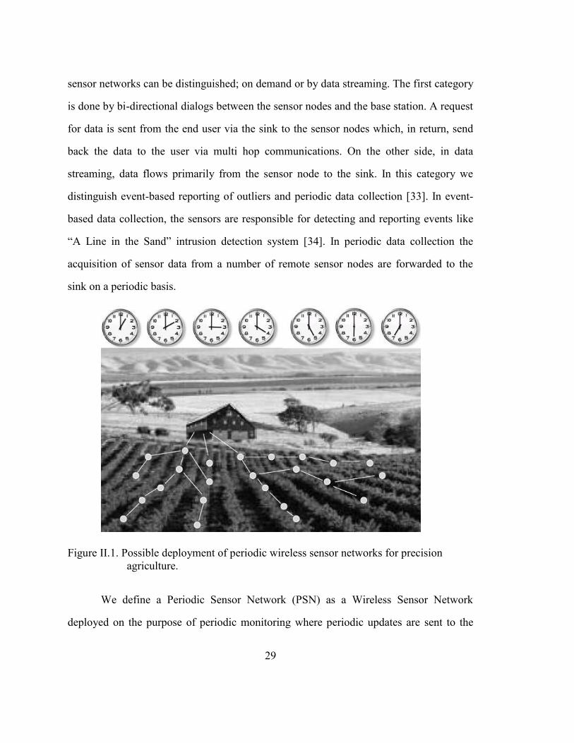
Figure II.1. Possible deployment of periodic wireless sensor networks for
precision agriculture..........................................................................29
Figure III.1. Naïve approach. ...............................................................................49
Figure III.2. Dynamic approach. ..........................................................................50
Figure III.3. The Behavior Curve Function ...........................................................54
Figure III.4. Sensor Nodes deployed in Intel Berkely Research Lab ....................56
Figure III.5. Snapshot of real data ........................................................................57
Figure III.6. The sampling rate adaptation for SMAX=250 ................................58
Figure III.7. The sampling rate adaptation for SMAX=150 ..................................58
Figure III.8. The energy consumption for SMAX=250 .........................................58
Figure III.9. The energy consumption for SMAX=150 .........................................58
Figure IV.1 WSN Taxonomies .............................................................................62
Figure IV.2 Flat Topology Architecture ..............................................................64
Figure IV.3 Cluster Based Topology architecture. Clusters boundaries referred by
dotted line..........................................................................................65
Figure IV.4 Tree based topology ..........................................................................66
Figure IV.5 chain based topology ..........................................................................67
Figure IV.6. Tree based data aggregation scheme.................................................70
Figure IV.7. Percentage of total data sent to the aggregator ..................................77
Figure IV.8 Second Tier Data Aggregation ...........................................................78
Figure IV.9. Energy Consumption ........................................................................80
Figure V.1 Percentage of total data sent to the aggregator ....................................97
Figure V.2 Percentage of deleted sets, δ= 0.01 ......................................................98
Figure V.3 Percentage of deleted sets, δ= 0.05 ......................................................99
Figure V.4 Percentage of deleted sets, δ= 0.07 ......................................................99
Figure V.5 Percentage of lost measures, δ= 0.01.................................................100

xx
Figure V.6 Percentage of lost measures, δ= 0.05.................................................100
Figure V.7 Percentage of lost measures, δ= 0.07.................................................101
Figure V.8 Received Measure (Temperature) .....................................................103
Figure V.9 Received Measure (Humidity)...........................................................104
Figure V.10 Data accuracy (Temperature) ..........................................................104
Figure V.11 Data accuracy (Humidity) ...............................................................105
Figure V.12 Total energy dissipation ...................................................................106
Figure.VI.1 K-Mining similar prefix sets in wsn .................................................118
Figure VI.2 K-means example .............................................................................123
Figure VI.3 Distribution of sensors in clusters, day= 1, delta=0.07 ....................125
Figure VI.4 Distribution of sensors in clusters, day= 1, delta=0.1 ......................125
Figure VI.5 Distribution of measurements in clusters based on K-means on data
source ..............................................................................................126
Figure VI.6 Similarity sets, delta=0.07 ................................................................127
Figure VI.7 Similarity sets, delta=0.1 ..................................................................127
Figure VI.8 Data accuracy, delta=0.07 ................................................................127
Figure VI.9 Data accuracy, delta=0.1 ..................................................................127
FigureVI.10 Running time, k= 4, delta=0.07 .......................................................128
FigureVI.11 Running time, day= 1, delta=0.07 ...................................................128

21
Chapter I Introduction
The need to monitor wide range of application areas has risen significantly during
the past years. To answer such demand, wireless sensor networks have been deployed
sporadically all over fields of application. Such deployment has failed to account the
erroneous and limited nature of these networks in terms of power and infrastructure.
Lured with such deficiency, researchers from all over the world have gained exponential
interest in improving wireless sensors network lifetime. The mission of WSN became
vast and wide spanning into various industrial, environmental and power arenas. A
typical topography of a sensor network is distributed redundantly in thousands over a
deployment site. Such redundant volume is required to ensure the cooperative sensors
readings reliability. Each sensor node has a separate sensing, processing, storage, and
communication unit. The sensing unit is primarily concerned with collecting data from its
work environment and the microprocessor processing unit handles the tasks. Memory is
used to store temporary data or data generated during processing whereas the
communication unit mainly interacts with the environment.
Physical resources constraints have to be taken into considerations in a wireless
sensor network: due to the limited bandwidth of wireless links connecting sensor nodes,
communication should be carefully tackled in order to avoid variable latency and dropped
packets. Sensor nodes are powered by a battery which supplies energy; however its
lifespan is tightly limited which makes energy optimization a major consideration that
affects the lifetime of a wireless sensor network. Finally, sensors computation power and
memory size are other issues that could hinder any data processing algorithm.
The major challenge that faces wireless sensor network implementation is
improving the lifetime of the network; in other words managing efficiently the battery

22
and power consumption. Extensive researches have focused on such task as it is difficult
and cost ineffective to recharge the battery [1][2]. Energy is mainly consumed during
data transmission from the source node to the sink (gateway). Then, sensor node is not
expected to carry huge amount of data or complex computations. As a result, packet
transmission is one of the core issues to address in order to reduce energy consumption
by mainly reducing the size of the packets transmitted.
Data collection from sensor networks can be on demand or by streaming. The first
is done by bi-directional dialogs between the sensor nodes and the base station. A request
for data is sent via the sink to the sensor nodes which, in return, sends back the data to the
requester via multi hop communications. On the other hand, by using streaming, data
flows primarily from the sensor node to the sink. We distinguish the periodic sampling
and the event driven data models. In periodic sampling, data is reported from the sensors
on periodic basis while in event driven model, an event triggers the generation of data.
Intrusion detection, battlefield gas detection are good example of applications answered
by the event driven sensor networks whereas the periodic model is the best for
applications that needs continuous monitoring like environmental or health monitoring.
This thesis focuses on ”periodic sampling” data model in sensor networks, where
the collection of sensor data from a number of remote sensor nodes is done on a periodic
basis. This data model is appropriate for applications where certain conditions or
processes need to be monitored constantly, such as the temperature in a conditioned space
or pressure in a pipeline. This type of network is called periodic wireless sensor network.

23
I. MAIN CONTRIBUTION
Our work focuses on overcoming the challenges imposed by periodic WSN
through data management while preserving the quality of the data. In fact, battery power
is a main limitation imposed by a wireless sensor network. As a result, saving resource
expensive transmission becomes a must. It is commonly understood that newest current
applications require data processing with temporal constraints in their tasks. Moreover,
periodic applications require querying processed data and real-time storage adding new
challenge to WSN. Data Management on the node level will ensure the usefulness of
every reading, thus reducing packet transmission size which consequently optimizes the
energy consumption. In such periodic networks, data collection, data aggregation and
data mining constitute the main components of data management. The listed phases in
periodic sensor data management are the pillars of interest in this thesis which analyzes
the existing and suggests efficient and improved algorithms.
A. Data Collection
Data collection from remote terrain and transmission of the information to the
sink is a fundamental task in periodic sensor networks. The “periodic sampling” data
model is characterized by the acquisition of sensor data from a number of remote sensor
nodes which are forwarded to the sink on a periodic basis. The sampling period depends
mainly on how fast the condition or process varies and what intrinsic characteristics need
to be captured. There are couple of important design considerations associated with the
periodic sampling data model.
The network is powered by a short lived battery which makes energy
consumption and efficiency a major challenge to look out for. Therefore, in order to keep
the networks operating for long time, adaptive sampling approach to periodic data

24
collection constitutes a fundamental mechanism for energy optimization. The key idea
behind this approach is to allow each sensor node to adapt its sampling rates to the
physical changing dynamics. In this way, over-sampling can be minimized and power
efficiency of the overall network system can be further improved. This thesis proposes an
efficient adaptive sampling approach based on the dependence of conditional variance on
measurements that varies over time. Then, it proposes a multiple levels activity model
that uses behavior functions modeled by modified Bezier curves to define application
classes and allow for sampling adaptive rate.
B. Data Aggregation
While developing a new technique that addresses the data collection, huge data
volumes generated periodically constitutes an intrinsic consideration in periodic sampling
data model. The most critical design issue at this stage is the phase relation among
multiple sensor nodes. Redundant data exists at this phase leading to huge packet size
which overheads the network and depletes the energy thus reducing the life cycle of the
network. Hence, in periodic sensor networks two neighboring nodes operate with
identical or similar sampling rates so redundant packets from the two nodes are likely to
happen repeatedly. It is essential for sensor networks to be able to detect and clean
redundantly transferred data from the nodes to the sink.
This thesis introduces a periodic hierarchical data aggregation model to achieve
this goal. Two layer algorithms are introduced: at the node level and at the aggregator
level. These algorithms aim to optimize the volume of data transmitted thus saving
energy consumption and reducing bandwidth on the network level.
At the first level, a simple process aggregate data on a periodic basis avoiding each
sensor node to send its raw data as is to the base station.

25
At the second level, “data aggregator“ sensor node collects the information from its
associated nodes where a new part of the filtering aggregation problem is explored. The
algorithm at this level identifies the similarity between data sets generated by neighboring
nodes and sent to the same aggregator. The objective is to detect similarities between
near sensor nodes, and integrate their captured data into one record while preserving
information integrity. In this context two techniques are studied: the first technique
suggests an algorithm to be applied on the level of the aggregator node itself taking into
consideration the number of occurrence of each measure; the second one suggests a new
prefix filtering method to study the sets similarity in sensor networks. Many optimization
techniques are also proposed to rightfully exploit the ordering of measurements according
to their frequencies and for early termination of sets similarity computing.
C. Data Mining in sensor networks
With the challenging data management phases in periodic sensor networks, the
large set of collected and aggregated data constitute ideal candidates for data mining
techniques. Numerous data mining applications deal with high-dimensional data,
however they impose a high computational cost which is not supported by sensor
network. Limitation in terms of available energy for transmission, computational power,
memory, and communications bandwidth are the main challenges of the sensor
network for data mining applications. The presented data aggregation phase will
constitute the preprocessing step to get the perfect data set to be mined in an acceptable
timeframe.
Data mining is a perfect tool to analyze data, categorize it and summarize the
relationships identified. Our approach will adopt this tool on the level of the aggregator
allowing it to send only useful information to the base station. The weight collected from

26
the first step will constitute the optimization key of a data mining algorithm (FP_Tree).
Our approach avoids the scanning procedure by working on a different structure resulting
from the output of the data cleaning algorithm applied on the level of the aggregator.
Another data mining algorithm has been also customized to respect the constraint
imposed by wireless Sensor Networks: K-Means. Our objective is to use the prefix
filtering to optimize the data mining algorithms in sensor networks. We applied K-means
on the prefix cleaned sets results of our data aggregation algorithm.
II. THESIS STRUCTURE
The rest of this thesis is structured as follows:
The second chapter introduces the periodic sensor network and its main objectives and
discuss the technological and data management challenges existing in periodic sensor
networks. A number of periodic sensor networks applications are also reviewed via some
existing examples.
Chapter III focuses on the adaptive data collection in periodic sensor networks to allow
each sensor node to adapt its sampling rates to the physical changing dynamics. An
efficient adaptive sampling approach based on the dependency of conditional variance on
measurements that varies over time is proposed. Then, a multiple levels activity model
that uses behavior functions modeled by modified Bezier curves to define application
classes and allow for sampling adaptive rate is suggested.
Chapter IV introduces as a first step the aggregation technique applied on a periodic basis
at the first level which is the source node level. At the source node level, we look at
specified intervals at each data measured and periodically clean the data taking into
consideration the number of occurrences of the measures. A second level of data
aggregation is performed between groups of nodes called aggregator. This algorithm will

27
not tolerate the effect of the information that each data measurement provides by
preserving the weight of each measure. The result set will constitute a perfect drill to
mine without high CPU activities allowing us to send only the information to the sink.
In chapter V, we shift gears to reducing measures redundancy by identifying near
duplicate nodes that generate similar data sets. A tree based bi-level periodic data
aggregation approach implemented on the source node and on the aggregator levels has
been considered. The problem of finding all pairs of nodes generating similar data sets
such that, similarity between each pair of sets is above a threshold t, have been explored.
We propose a new frequency filtering approach and several optimizations using sets
similarity functions to solve this problem. The obtained results show that our approach
offers significant data reduction by eliminating in network redundancy and outperforming
existing filtering techniques.
In chapter VI, this thesis tackles the problem of adapting distributed “k-means”
clustering, a data mining algorithm, on the prefixes sets in order to cluster observations
into groups of related data without any prior knowledge of the relationships between the
prefixes sets. The main interest in this chapter was to design an efficient prefix mining
algorithm in sensor network, both from a statistical and computational point of view. This
chapter addressed the energy problem in sensor network and the problem of mining
prefix item sets instead of mining the whole set of data. Simulation results have been
compared with other model and techniques.
The Last Chapter concludes this work with some aspects of suggested future research
work.

28
Chapter II Periodic Wireless Sensor Networks
Recent technological developments in the miniaturization of electronics and
wireless communication technology have led to the emergence of Wireless Sensor
Networks which will greatly enhance environment monitoring and lure techniques for
periodic taking measurements of some historically unstudied phenomenon. This is
particularly important in remote or menacing environments where many essential
processes have rarely been studied due to their inaccessibly. In this chapter, we attempt to
introduce a periodic sensor network and its main objectives. We review a number of
periodic sensor networks applications via some existing examples. Then we discuss the
technological and data management challenges in periodic sensor networks.
I. WHAT IS A PERIODIC SENSOR NETWORK (PSN)?
Wireless sensor networks (WSN) are composed of a large number of low cost
sensor nodes deployed over a geographical area for a specific monitoring [31]. Typically,
a sensor node is a tiny device that includes three basic components: a sensing subsystem
for data acquisition from the physical surrounding environment, a processing subsystem
for local data processing and storage, and a wireless communication subsystem for data
transmission. In addition, a power source supplies the energy needed by the device to
perform the programmed task [32]. Wireless sensor networks have a multitude of
applications, ranging from environmental to military domains. These applications include
contamination tracking, habitat monitoring, health monitoring, traffic monitoring,
building surveillance and monitoring, industrial and manufacturing automation,
distributed robotics and enemy tracking in the battlefield [31].
The main common task of a sensor node is monitoring some phenomena and
relaying data toward a base station called “Sink”. Two categories of data collection in
29
sensor networks can be distinguished; on demand or by data streaming. The first category
is done by bi-directional dialogs between the sensor nodes and the base station. A request
for data is sent from the end user via the sink to the sensor nodes which, in return, send
back the data to the user via multi hop communications. On the other side, in data
streaming, data flows primarily from the sensor node to the sink. In this category we
distinguish event-based reporting of outliers and periodic data collection [33]. In event-
based data collection, the sensors are responsible for detecting and reporting events like
“A Line in the Sand” intrusion detection system [34]. In periodic data collection the
acquisition of sensor data from a number of remote sensor nodes are forwarded to the
sink on a periodic basis.
Figure II.1. Possible deployment of periodic wireless sensor networks for precision
agriculture.
We define a Periodic Sensor Network (PSN) as a Wireless Sensor Network
deployed on the purpose of periodic monitoring where periodic updates are sent to the

30
sink from the PSN, based on the most recent information sensed from the physical
parameter. PSNs are typically arrays of sensor nodes interconnected using a radio
communication network which allow their data to reach the sink. They are used for
applications where certain conditions or processes need to be monitored constantly, such
as the temperature in a conditioned space or pressure in a process pipeline. An example
of periodic sensor network is shown in Figure II.1. It depicts a precision agriculture
deployment. Hundreds of nodes scattered throughout a field detect temperature, light
levels and soil moisture at hundreds of points. Every five minutes, each node takes one
data measurement and each one hour communicates its data over a multi-hop
communication to the end user for analysis.
II. PERIODIC SENSOR NETWORKS APPLICATIONS
Periodic sensor networks are used in several applications and for many purposes
[118]. The simplest of these are weather stations, and more complex examples include
seismic monitoring. We can find microclimate monitoring, water quality monitoring,
cattle monitoring, and other monitoring applications. In the reminder of this section, we
give an overview of existing periodic sensor networks applications.
The Georgia Automated Environmental Monitoring Network is a periodic weather
sensor network. The data are collected every 1 second and summarized at 15 minutes
intervals and at midnight a daily summary is calculated. The data are processed
immediately and disseminated via the Internet [35] and analyzed within a cyber-
infrastructure system [36]. Another example is the Snow-pack Telemetry (SNOTEL)
project which uses meteor burst communications technology to collect and communicate
data in real-time [37]. These SNOTEL are generally located in remote high-mountain
watersheds where access is often difficult or restricted. They are designed to operate

31
unattended and without maintenance for a year and are battery powered with solar cell
recharge. The main objective in [46] is to provide reliable, long-term monitoring of
rainforest ecosystems. The target was a rainforest area in South-East Queensland
(Springbrook, Australia) which had a high priority for monitoring the restoration of
biodiversity. The first phase of the project was to develop a better understanding of the
challenges in deploying long-term, low-power PSNs in rainforest environments.
The Tropical Atmosphere Ocean Project (TAO) which collects real-time data
from 70 moored ocean buoys in the Pacific Ocean to study El Niño processes [38]. The
system begun during the 1970s, and today the data is transmitted by satellite to the
Internet. However, existing infrastructure can be adapted to support local periodic sensor
networks. The CORIE project [39] integrates a real-time periodic sensor network, a data
management system and advanced numerical models to understand on the spatial and
temporal variability of the Lower Columbia River, USA. This project combines
environmental observation with forecasting. On a larger scale from this is the US
Geological Survey (USGS) NWIS web water data which has 1.5 million stations across
the USA providing real-time and sampled data on line [40]. The purpose of the project in
[45] was to monitor the salinity, water table level, and water extraction rate at a number
of bores within the Burdekin irrigated sugar cane growing district. This is a coastal region
and over extraction of water leads to saltwater intrusion into the aquifer. The area we
monitored was approximately 2 - 3 km2. The PSN had to operate unattended; it was very
sparse with very long wireless transmission ranges (with average link length over 800 m).
One simplification was that many nodes could be mains powered (since they were co-
located with pumps). Another PSN was deployed to measure vertical temperature profile
at multiple points on a large water storage that provides most of the drinking water for the
city of Brisbane, Australia. The data, from a string of temperature transducers at depths

32
from 1 to 6 m at 1-m intervals, provide information about water mixing within the lake
which can be used to predict the development of algal blooms [50].
The Volcano Tungurahua project [41] used a wireless periodic sensor networks to
monitor volcanic activity by specially-constructed microphones to monitor infrasonic
(low-frequency acoustic) signals emanating from the volcanic vent during eruptions. The
network gathered over 54 h of continuous infrasound data, transmitting signals over a 9
km wireless link back to a base station at the volcano observatory. The GlacsWeb project
[42] which uses a wireless sensor network to understand sub-glacial processes using
sensor nodes embedded in the glacier and sub-glacial sediment. From August 2004 to
August 2005 it collected the equivalent of 859 days of probe data (36,078 sensor
readings) on sub glacial water pressure, case stress, temperature, tilt angle and resistivity.
From this they were able to reconstruct how sub glacial processes operated over the year
in order to understand the relationship between glacier dynamics and climate change.
Other periodic sensor networks projects have been developed by the Centre for
Embedded Network Sensing at University of California, Los Angeles (UCLA) which has
over eight projects (like the Great Duck Island project) in different environments [43]. In
these projects, sensor nodes are responsible of measuring generic parameters such as
incoming solar radiation, air temperature and humidity, soil temperature and soil
moisture. They are mostly installed within a small area (up to 2 km2), and report back to a
central base station either directly or via a relay. The authors in [44] describes how data
are collected by one node and shared with others, these nodes can react and change their
behavior on the basis of this shared data. They define this behavior as a sensor web.

33
III. CHALLENGES FOR PERIODIC SENSOR NETWORKS
Extracting periodic data gathered by sensor nodes deployed in different (maybe
inaccessible) locations involves some unique challenges. These issues can be common to
the traditional wireless sensor networks.
Power consumption: The only power source of a sensor node often consists of a
battery with a limited energy budget. In addition, it could be impossible or inconvenient
to recharge the battery, because nodes may be deployed in a hostile or unpractical
environment. On the other hand, the PSN should have a lifetime long enough to fulfill the
application requirements.
Communication: The bandwidth of wireless links connecting sensor nodes is
usually limited, and the wireless networks connecting sensors provide only limited
quality of service such as variable latency and dropped packets. On the other side, radio
communications success is unpredictable in wet and windy locations. For example, radio
losses are not negligible in glacier ice and other environments, e.g. leaf cover changes in
forest habitats. The ability to alter transceiver power and the use of lower frequency or
acoustic fallback systems is commonly used.
Computation: Sensor nodes have limited computation power and memory sizes
that restrict the types of data processing algorithms that can be deployed and intermediate
results that can be stored on the sensor nodes.
Scalability: Periodic sensor networks deployed large number of sensor nodes in
order to monitor some phenomenon. Any node wishing to communicate with other nodes
generates more packets than its own data packets. These extra packets are generally
called control packets or network overhead. Moreover, the larger the network the more
potential there is for interruption in communication links, resulting in the creation of
more control packets. In summary, more overhead is unavoidable in a larger scale

34
periodic sensor network if the communication paths are to be kept intact. Since the
available overall bandwidth is limited, an increase of overhead results in the decrease of
usable bandwidth for data transmission. As the network continues to grow, only a very
small amount of bandwidth will be left for application data transmission.
Remote management: Sensor nodes in isolated locations cannot be visited
regularly so remote access is essential. Bugs need fixes, subsystems might need shutting
down and schedules changed. For example, the Duck Island project found that their
sensors could short circuit their power when wet. Custom communications make remote
access more complex because normal logins and routing are not available. More software
development and failure scenario testing is required in order to achieve good remote
management.
Security: Although security is a necessity in other types of networks, it is much
more so in sensor networks due to the resource-constraint, susceptibility to physical
capture, and wireless nature. Security issues are important at all levels of periodic and
event driven sensor networks from physical to data interference. PSN can cope with the
loss of one or more nodes due to failure or damage. Data may need to be protected
against deliberate and accidental alteration. However security should not be used to
hamper public access to information. A balance between security and information needs
to be reached so that all parties can trust the deployed PSN; this will dramatically affect
their development and implementation.
Data management: The main difference between the traditional event driven
sensor networks and PSN is the huge amount of data collected from the field of
monitoring. In the event driven model, the kind of data collection is less demanding in
terms of the amount of wireless communication, since local filtering is performed at the
sensor nodes, and only events are propagated to the base station. In the next section, we

35
introduce data management in periodic sensor networks and its challenges from the
collection to the decision making.
IV. DATA MANAGEMENT CHALLENGES IN PSN
Massive and heterogeneous data collected from periodic sensor networks brings
the data management challenges. The traditional approach of migrating raw data to
centralized points for data storage and analysis may incur debilitating communication and
high energy costs. In this section, we will discuss different challenges in the data
management field for periodic sensor networks.
Data collection: Periodic data collection in periodic sensor networks enables
complex analysis of data, which may not be possible with query processing because of
the great amount of the collected data. Researchers’ strategies are directed to minimize
the amount of data retrieved (communicated) by the network without considerable loss in
fidelity (accuracy). The main objective of this reduction is first to increase the network
lifetime and then to help in analyzing data and making decision. Using compression
schemes is one way to reduce the amount of data that needs to be transferred to the base
station. Another method is to scale periodic wireless sensor networks to the size of the
system/region under study and sample data at frequencies equivalent to physical
phenomenon changes. Periodic sensor networks with these properties can provide the
appropriate fine-grain information needed for accurate modelling and prediction.
Data delivery latency: Real-time delivery is very important in most applications
of periodic sensor networks. Therefore, reducing latency is very important. The periodic
data collected from the sensor nodes are expected to be delivered to the end user with a
minimum latency. For example, snow monitoring data must be delivered in the order of
hours to days, but not weeks. The major challenge for periodic sensor networks lies in the

36
fact that this latency guarantee need to be met in the presence of hard power constraints
and limitations of radio connectivity. The data needs to be delivered via a multi-hop
communication using radio transceiver with limited communication range (about 30
meters). This problem warrants an ultra-low-power solution that not only meets the data-
delivery latency requirements, but also maximizes the network lifetime simultaneously.
Data integrity and quality: To ensure a good understanding of the monitored
phenomenon, it is imperative to assess the quality of the data gathered by periodic sensor
networks before presenting them to the users. The first challenge is about ensuring
temporal integrity. PSN applications require periodic measurements to be time-stamped
to an accuracy of seconds to milliseconds. Thus, assigning accurate timestamps to the
collected measurements is a non-negligible issue in PSN. Apart from ensuring temporal
integrity, the data gathered by such network contains a lot of missing values and are
inherently noisy. Sensor calibration is vital for high quality data collection. Furthermore,
it is crucial to apply methods that are robust and can deal with data of such nature.
Finally, defining the exact source of sensor data is important when they are analyzed.
This data source will need to be preserved without placing too much burden on the users.
Big data volumes management: Periodic sensor networks produce immense
amount of data continuously. For example, a 50 node deployment that collects data every
minute from 10 different sensing fields will produce over 26 million records over a year
period. Knowing that sensor nodes have limited memory and computational resources
and cannot save all the collected data. Important for data processing in PSN will be
intelligent data reduction at individual sensor nodes through the computation of measures
aggregates. In addition to these local computations, we need to be able to process and
combine received data from several sensor nodes. This can be done by an effective data
aggregation technique. Another major challenge with sensor data is converting raw

37
sensor values into final usable data and ready to make decisions. This will require
concerted efforts to make simple and efficient data mining on periodic collected data with
different levels of detail and low latency.
Distributed data management: Sensor nodes collect the data about the
environment from different locations and different sources in order to send it to the end
user for a variety of analysis. Unfortunately, post analysis of the data extracted from the
periodic sensor networks incurs high sensor communication cost for sending the raw data
to the base station and at the same time runs the risk of delayed analysis. To overcome
this, distributed data management algorithms have been proposed to deal with the data on
site. These algorithms utilize the computing power at each node to do some local
computations and then exchange messages with its neighbors leading to a consensus
regarding a global model. These algorithms reduce the communication cost vastly and
extend the whole network lifetime.
V. CONCLUSION
In this chapter, we introduced the periodic sensor network which is the core
interest of this thesis. Several applications are in need of periodic sensor network in order
to answer crucial objectives like monitoring, preventing or forecasting. As presented,
sensor network architectures include some design aspects imposing big challenges when
working with them. Energy efficiency is the primary challenge to increase the network
lifetime. Therefore, data management techniques are an essential building blocks aiming
to reduce energy consumption by reducing the number of transmissions required. This
chapter highlights the main challenges of data management in periodic sensor networks
that need to be accounted for. The upcoming chapters will tackle in details the data

38
management in periodic sensor networks by introducing new overcoming suitable
approaches.

39
Chapter III Adaptive Data Collection in periodic sensor networks
Data collection from unreachable terrain and then transmit the information to the
sink is a fundamental task in periodic sensor networks. However, in order to keep these
networks operating for long time, adaptive sampling approach to periodic data collection
constitutes a fundamental mechanism for energy optimization. The key idea behind this
approach is to allow each sensor node to adapt its sampling rates to the physical changing
dynamics. In this way, over-sampling can be minimized and power efficiency of the
overall network system can be further improved. In this chapter, we present an efficient
adaptive sampling approach based on the dependence of conditional variance on
measurements that varies over time. Then, we propose a multiple levels activity model
that uses behavior functions modeled by modified Bezier curves to define application
classes and allow for sampling adaptive rate. The proposed method was successfully
tested in a real sensor data set.
I. INTRODUCTION
Due to the large amounts of data generated by wireless sensor networks(WSN),
collection of sensing data to be forwarded from the sensor nodes to a central base station
constitute a major process for WSN. This process is known as Data Collection.
Unfortunately, the transmission of large quantities of data is a threat on the lifetime of the
sensor network due to the limited energy resources of the sensor nodes. On the other hand
most of the applications require all the data generated and doesn’t tolerate any loss of
detail as to reach the accuracy required. For instance, we can list the structural health
monitoring application [3] that requires more than 500 samples per second to efficiently

40
detect damage. All of this makes the data collection in WSN an interested area of
research where transmission of data should be studied carefully.
The “periodic sampling” data collection model is characterized by the acquisition
of sensor data from a number of remote sensor nodes then pushing them to the sink on a
periodic basis. These periodic models are used for applications where certain conditions
or processes need to be monitored constantly, such as the temperature or pressure, etc. As
seen in the previous chapter, some examples of these applications include the observation
of nesting patterns of storm petrels at Great Duck Island [4], measuring light intensities at
various heights in a redwood tree [5] and logging temperature and humidity in the canopy
of potato plants for precision agriculture [6]. The sampling period in periodic data
collection model depends mainly on how fast the condition or process varies and what
intrinsic characteristics need to be captured. As seen in chapter II, there is couple of
important design considerations associated with the periodic sampling data model. One of
them is the over-sampling. For instance, the dynamics of the monitored condition or
process can slow down or speed up; if the sensor node can adapt its sampling rates to the
changing dynamics of the condition or process, over-sampling can be minimized and
power efficiency of the overall network system can be further improved.
II. RELATED WORK
Predicting the values measured either in source node or sink in a periodic wireless
sensor networks is one of the data reduction methods to reduce the amount of data sent by
each node. Many researches fall in this area aiming to reduce the communication
overhead by selecting a subset of the data produced and reconstructing all the original
data with some level of accuracy. Some work [10][21] that guarantees that the data

41
maintained at the central server is within a certain interval of the actual sensor readings
and node, reports their readings to the server in case the value is outside this interval. [29]
proposed an energy efficient clustering and prediction protocol which uses mobile sink to
route the path efficiently. On the other hand, we should highlight that time and space are
two main factors based on which prediction and adaptive sampling can be performed
since data is correlated in both time and space.
Hence, adaptive sampling helps to reduce the number of samples by exploiting either
spatial, temporal or spatio-temporal correlations between sensed data. [11], [12] rely on
the time factor to perform data reduction while [13], [14] count on the space domain.
Some few approach count on the temporal and spatial domain [20], [16]. The below
elaborates the different prediction model approaches existing for data collection in
periodic wireless sensor networks.
A. Time Series Approach
As a record of the target trajectory, a time series of historical target positions is
transferred among the sensor nodes with sensing tasks. When the current target position
is obtained, the historical target is also available in the active sensor nodes so that target
forecasting can be performed.
Reporting approximations of sensor readings at regular time intervals is required
in many applications of wireless sensor networks. Hence, Time series prediction
techniques have been adopted as an effective technique to reduce the communication
effort while preserving the accuracy of the collected data. The target is often predicted by
a number of sensor nodes and a Fisher information matrix (FIM) is used to evaluates the
target localization error [17]. Measurements of the target are produced by using time
series of historical target positions transferred among the sensor nodes with sensing tasks.
Time series analysis in WSN implements the target position forecasting through the
known target trajectory. [49] processes the time series by empirical mode decomposition
introduced in [18] described by ARMA models adaptively. Then, the forecasted results of

42
each component are combined to forecast the target position. The operation energy
consumption of sensor node is optimized using a probability awakening approach noting
that an anti-colony optimization (ACO) [19] is introduced to optimize the routing scheme
for the next sensing period.
On the other hand, Goel and Imilienski [16] visualize the sensor readings as an
optical image which let them adapt the MPEG standard for video compression and
generate a prediction model so the readings is sent to the sink only if it differs
significantly from the predicted model. The prediction model in this case is only valid for
a specific period of time. Deshpande et al. [15] propose a similar model driven approach
where the temporal prediction model is learnt from historical data then use to predict the
new sensor readings in the current time period. Guestrin et al. [13] use a kernel linear
regression to build a model of the data by letting the nodes transmit only the changes on
the level of the model coefficients instead of the raw data. In [14], the subsets are used in
a round robin fashion by relying on a single subset identified from several nodes subsets
to predict the readings of the remaining subsets. In this approach, only one subset is
solicited at a time which leads to energy savings.
A temporal correlation of data is used also in [22], where the authors propose an
adaptive sampling scheme suitable to snow monitoring for avalanche forecast. Some
approaches are based on the prior identification of some parameters like Dual kalman
filter that perform linear prediction by sending updates to a central server only when the
prediction error exceeds some given threshold. Many kalman filters as the number to
remote sources run in parallel at the central server in order to reconstruct the phenomenon
observed on the source node and reconstruct the model based on the data received or the
computed predictions. A drawback of this approach is its dependency on the model of the
observed phenomenon that should be provided by both server and node to the filter. [23]
Overcomes this limitation by proposing least mean square (LMS) an adaptive algorithm

43
that doesn’t require nodes to be assisted by a central entity to perform prediction, since no
global model parameters need to be defined. However this algorithm consider a loss-free
communication links between sink and source and rely only on single sensor reading in
the time domain.
All the described approaches required a central entity that collects the sensor
readings from neighboring nodes for the extraction of the prediction model. Therefore the
sensor nodes are dependent on this central entity to ensure the data reduction which
means that all these approach are centralized. To note also that this model may suffer
from inaccuracy since it might become outdated.
B. Spatial Approach
Other existing methods are limited to only space correlation and based on
grouping nodes into clusters. Spatial data correlation is used in [24], where a back casting
scheme is proposed. Mainly, nodes deployed with sufficient density do not have to
sample the sensed field in a uniform way. In fact, more nodes have to be active in the
regions where the variation of the sensed data quantity is high. In this work a cluster
based method is used to group sensors in clusters, each managed by a cluster-head. The
authors in [25] define a spatial Correlation based Collaborative MAC protocol (CC-
MAC) that regulates sensor node transmissions so as to minimize the number of reporting
nodes while achieving the desired level of distortion. In [26] a TA-PDC-MAC protocol is
proposed, a traffic adaptive periodic data collection MAC which is designed in a TDMA
fashion. This work is designed in the ways that it assigns the time slots for nodes activity
due to their sampling rates in a collision avoidance manner. Adaptive Sampling
Approach to Data Collection (ASAP) is proposed in [27]. This technique splits the
network into clusters. A cluster formation phase is performed to select cluster heads and
select which nodes belong to a given cluster. The metrics used to group nodes within the

44
same cluster include the similarity of sensor readings and the hop count. Then, not all
nodes in a cluster are required to sample the environment. Adaptive sampling techniques
are very promising, because of their efficiency to optimize energy consumption and the
network overload. However, most of the previous proposed solutions are implemented in
a centralized manner that requires rather huge computations and communications.
C. Spatio-Temporal Approach
Some works [28], [16], [30] exploit the spatio-temporal correlation among data
and predict the measurements from the subset of sensor reading identified for this
purpose. The predicted data solve the issue of delivering the whole data to the sink, thus
reducing communication.
In this thesis that specifically addresses periodic sensor networks; we propose a
non-complex distributed adaptive sampling algorithm that is based on the sensed data
variation. Moreover, we take into account the application criticality and propose a model
that dynamically defines multiple levels of sampling rate corresponding to how many
samples are captured per unit of time. The final goal is to provide the necessary
algorithmic support for environmental surveillance applications to express their
objectives.
The rest of this chapter is organized as follows. In section II we present our model
of adaptive sampling rate based on the variance study. In section III we describe how to
integrate the application criticality level in order to adapt the sampling rate. Section IV
presents our experimental results based on real data readings. We show that our model
performs well and allows to dynamically adapt its sample rate in order to save its energy
consumption. Finally we conclude with some few remarks.

45
III. ADAPTING SAMPLING RATE
A. Variance study
In this section we perform a statistical model allowing to compare means of
measures taken by a node in different periods. Based on this comparison a node will
adapt its sampling rate. With a period p a sensor node takes several measures of
temperature or humidity for example. To illustrate, we consider a sensor node n after J
periods. The objective is to compute the variation between periods after every new period
to adapt the sampling rate in function of the new variance. The variance between periods
may be thought of as a signal of measures differences. Therefore, we use the one way
ANOVA model to test whether or not the means of several periods are all equal and if the
variance differs from one period to another. We suppose that measures inside each period
J are independent, with mean and the variances of periods are equal . Then the measure’s variable can be written as follows: ⃗⃗
Where are the residual which are independent and are normally distributed following
N(0; ).
We denote by: ∑ ∑
∑∑
the mean and the variance in each period and the mean of all the J periods respectively.
The total variation (ST) is the within period variation (SR) and the between period
variation (SF). The whole idea behind the analysis of variance is to compare the ratio of
between period variance to within period variance. If the variance caused by the

46
interaction between the measures is much larger when compared to the variance that
appears within each period, then it is because the means aren’t the same. Let us consider:
∑ ∑ ∑ ∑ ∑ (1)
B. Mean’s period verification
In this section we present how each sensor after each period compares the means
and computes the variance to then adapt its rate. After a period j, each sensor node will
test the hypothesis that all the previous period means and the new one are the same or
not. Therefore we used the Fisher test, let
⁄ ⁄ (2)
If the hypothesis is correct then, F will have a Fisher distribution, with F(J - 1; N - J)
degrees of freedom.
The hypothesis is rejected if the F calculated from the measurements is greater than the
critical value of the F distribution for some desired false-rejection probability (risk α). Let
Ft = F1-α(J -1; N -J). The decision is based on F and Ft:
If F > Ft the hypothesis is rejected with false-rejection probability α, and
the variance between periods are significant
If F ≤ Ft the hypothesis is accepted.

47
C. Illustrative example
Consider the measures and periods as shown in the following table:
Periods (j) 1 2 3 4 5
1.51
1.92
1.08
2.04
2.14
1.76
1.17
1.69
0.64
0.90
1.41
1.01
0.84
1.28
1.59
1.56
1.22
1.32
1.39
1.33
1.54
1.04
2.25
1.49
1.30
0.75
1.26
0.69
0.62
0.90
1.20
0.32
0.73
0.80
0.90
1.24
0.82
0.72
0.57
1.18
0.54
1.30
1.66 1.17 1.46 0.88 0.88 = 1.189 0.175 0.144 0.115 0.123 0.074 7 8 9 8 10 N = 42
Table III.1: Measures Example
For α = 0.01 we have Ft = 3.83, after the fifth period we find F = 8.066 and after the
fourth period we find F = 7.43.
IV. ADAPTATION TO APPLICATION CRITICALITY
In periodic sensor networks and in order to save energy, it is desirable to be able
to adjust the sampling rate according to the applications requirements. If we are in the
context of critical applications, sensor nodes should speed up its sample rate faster than
sensor nodes in non-critical applications. In our approach we express the application
criticality by the r0 variable which can take values between 0 and a defined 1 representing
the low and the high criticality level respectively. Low level criticality indicates that the
application does not require a high sampling rate while a high level criticality does. Then,

48
according to the applications requirements, r0 could be initialized accordingly into all
sensors nodes prior to deployment.
To take into account the application criticality, a naïve approach would consist in
fixing the measure sampling rate of all sensor nodes to a given rate. As illustrated in
Figure III.1, we show how the sensor nodes capture speed can be regulated proportionally
to the dynamic risk level r0. For instance, a high criticality level pushes sensor nodes to
capture at near the maximum sampling rate capability. The idea behind this model is,
when the observed F become greater than threshold Ft (= F1−α ) the sampling rate is
balanced to the maximum sampling rate or to the minimum sampling rate in the other
cases. However, this simple approach presents some drawbacks:
(i) Setting sensor nodes to work at full capacity provides high number of taken
measures which need high bandwidth and leads to run out the sensor batteries and thus
reducing the network lifetime
(ii) Although setting the nodes at low capacity saves energy and extends the
network lifetime, it provides poor data quality where some important measures will be
missed.
(iii) Choosing a moderate sampling rate could balance between capture quality
and network lifetime but at the same time sensors cannot be fully exploited if it is
necessary and the physical changes are very dynamics.

49
Figure III.1. Naïve approach.
A. Dynamic sampling model
To fully exploit the sensor node capabilities we propose that a node sampling rate
depends on the result of the fisher test F as shown in figure III.2. Based on the results and
residual of the variance test described above, the idea is that when a node noticed high
variance differences, it can increase its sampling rate in order to prevent missing
important measures and decrease its sampling rate when the variance are lesser than the
threshold. In general, it is desirable to be able to adjust the sampling rate according to the
application’s requirements. In our approach we express the application criticality by the
quantitative variable r0 which can take values between 0 and 1 representing the low and
the high criticality level respectively. Low level criticality indicates that the application
does not require a high sampling rate while a high level criticality does. Then, according
to the application’s requirements, r0 could be initialized accordingly into all sensors
nodes prior to deployment. It is also possible during the network lifetime to dynamically
change r0 , in all sensor nodes or for a given subset only, if some kind of supervision and

50
control platform is available. In what follows we will define different application classes
which will determine a node’s sampling rate.
Figure III.2. Dynamic approach.
1) Influence on the F-ratio:
In this section, we discuss why the sampling rate increases when the F-ratio
increases. In fact, the greater the difference among the means, the higher is the F and the
greater the likelihood of obtaining variance differences. Hence, it is important to note that
a large F does not by itself convey why or how the means differ from each other. A high
F value can be found when the means for all of the groups differ at least moderately from
each other. Alternatively, a high F can be obtained when most of the means are fairly
similar but one of the means happen to be far removed from the other means. In this last
case, F ratio is influenced by group means, where the variances intra groups are very
different. In these two cases, the sensor node must increase its sampling rate to capture all
physical changes.
2) Application classes:
We can broadly classify applications into different categories based on their
criticality level. In our approach we define two classes of applications: high and low

51
criticality applications. This criticality level is represented by a mathematical function y =
f(r0,F) that we call BV (BehaVior) function inspired from [48]. This function can
oscillate from hyperbolic to parabolic shape as illustrated in Figure III.3:
• Values on the x axis are positive results of Fisher test. These values lie between
1 and Ft. We consider that Ft corresponds to the maximum sampling rate. Thus, if a node
finds F greater than Ft it puts its sampling rate to the maximum.
• The y axis gives the corresponding sampling rate based on the Fisher test results
on the x axis and the application criticality level (r0) (number of sensed measures per unit
of time).
We now present the contrast between applications that exhibit high and low
criticality level in terms of the BV function.
1) Class 1 ”low criticality”, 0 ≤ r0 < 0.5: this class of applications does not need
high sampling rate. This characteristic is represented by hyperbolic projections of x
values that are gathered close to zero (i.e. the majority of the sensors will preserve their
energy by sampling slowly).
2) Class 2 ”high criticality”, 0.5 ≤ r0 ≤ 1: This class of applications needs high
sampling rate. This characteristic is represented by a parabolic BV function. As
illustrated in figure III.2, most projections of x values are gathered close to the max frame
capture rate (i.e. the majority of nodes capture at a high rate).
3) The behavior function:
We use Bezier curve to model the BV function. Bezier curves are flexible and can
plot easily a wide range of geometric curves.

52
Definition III.1: Bezier Curve
The Bezier curve is a parametric form to draw a smooth curve. It is fulfilled
through some points P0, P1 ...Pn, starting at P0 going towards P1 ...Pn−1 and terminating at
Pn.
In our model we will use a Bezier curve with three points which is called a
Quadratic Bezier curve. It is defined as follows:
Definition III.2: Quadratic Bezier Curve
A quadratic Bezier curve is the path traced by the function B(t), given points P0 ,
P1 , and P2 .
B(t) = (1 − t)2 * P0 + 2t(1 − t) * P1 + t
2 *P2 . (3)
The BV function is expressed by a Bezier curve that passes through three points:
• The origin point (P0 (0, 0)).
• The behavior point (P1 (bx, by ))
• The threshold point (P2 (hx , hy )) where hx represents Ft and hy represents the
maximum sampling rate determined by the sensor node hardware capabilities.
As illustrated in Figure 3.3, by moving the behavior point P1 inside the rectangle
defined by P0 and P2, we are able to adjust the curvature of the Bezier curve. The BV
function describes the application criticality. It takes F value as input on the x axis and
returns the corresponding “sampling rate” on the y axis. To apply the BV function with
the Bezier curve, we modify this later to obtain y as a function of x, instead of taking a
temporal variable t as input to compute x and y. Based on the Bezier curve, let us now
define the ”BV function”:
Definition III.3: Bezier Curve function
The BV function curve can be drawn through the three points P0 (0, 0), P1 (bx , by)
and P2 (hx , hy ) using the Bezier curve as follows:

53
[ ] [ ]
{ (4)
Where √ {
4) The criticality level r0: As discussed above, the criticality level r
0 of an
application is given into the interval [0, 1]. According to this level, we define the
criticality function called Cr which operates on the behavior point P1 to control the BV
function curvature.
According to the position of point P1 the Bezier curve will morph between
parabolic and hyperbolic form. As illustrated in figure III.3 the first and the last points
delimit the curve frame. This frame is a rectangle and is defined by the source point P0(0,
0) and the threshold point P2(hx, hy). The middle point P1(bx, by) controls the application
criticality. We assume that this point can move through the second diagonal of the
defined rectangle

54
Figure III.3. The Behavior Curve Function
We define the Cr function as follows, such that varying r0
between 0 and 1 gives
updated position for P1:
[ ] [ ] [ ] ( ) {
Level r0 is represented by the position of point P1.
If r0 = 0, P1 will have the coordinate (hx, 0). If r
0 = 1, P1 will have the coordinate (0, hy).
B. Adapting Algorithm
The adaptive sampling rate algorithm operates in rounds where each round equals
m periods. For each round, every node decides to increase or decrease its sampling rate
according to the variance condition and the application risk. The algorithm is presented in
algorithm III.1.

55
Algorithm III.1: Adapting rate algorithm.
Require: m (1 round = m periods), Smax (maximum sampling speed), r0
Ensure: St (instantaneous sampling speed).
1: St ← Smax
2: while Energy > 0 do
3: for i = 1 → m do
4: takes measures at St speed
5: end for
6: for each round do
7: compute SR, SF and F.
8: find Ft
9: if F < Ft then
10: St ← BV (F, Ft , r0 , Smax ) (BV behavior function).
11: else
12: St ← Smax
13: end if
14: end for
15: end while
V. EXPERIMENTAL RESULTS
To verify our suggested approach, we conducted multiple series of simulations
using a custom Java based simulator. The objective of these simulations is to confirm that
our adaptive data collection technique can successfully achieve desirable results for
energy conservation in periodic sensor networks. Therefore, in our simulations we used
real readings collected from 45 sensor nodes deployed in the Intel Berkeley Research
Lab(see figure III.4) [47].

56
Figure III.4. Sensor Nodes deployed in Intel Berkely Research Lab
Every 31 seconds, sensors with weather boards were collecting humidity, temperature,
light and voltage values. In our experiments, we used a file that includes a log of about
2.3 million readings collected from these sensors. Figure III.5 shows a screen capture of
this file. Temperature is in degrees Celsius. Humidity is temperature corrected relative
humidity, ranging from 0-100%. Light is in Lux. Voltage is expressed in volts.
For the sake of simplicity, in this chapter we are interested in one field of sensor
measurements: the temperature. We performed several runs of the algorithms. In each
experimental run, each node reads periodically real measures and adapts its sampling rate
after each round according to its BV function. We evaluated the performance of the
algorithm using the following parameters: a) the time t; b) m the number of periods per
round; c) the application criticality level (r0). We employ two metrics in our simulations:
the instantaneous sampling speed after each round;
The overall energy dissipation

57
Figure III.5. Snapshot of real data
The main goal here is to show how our approach is able to adapt the sampling rate of the
sensor nodes according to the changing dynamics of the environment and to the
application criticality level. Our simulation results were obtained for the following
parameters:
- a period is equal to 500 measures (' 4 hours)
- SMAX = 150 or 250
- m = 2,
- α= 0.05
- r0 = 0.2 and 0.9
Figures III.6 and III.7 confirm our previous analysis and show that the sampling rate is
changing along the time and is able to adapt itself to application criticality i.e. r0. Now
from an energy preservation point of view (figures III.8 and III.9), if we assume that each
sensor has an energy level arbitrarily fixed to 5000 units and that each measure consumes
0.125 unit our simulation results are again very encouraging. For example, for r0 = 0.2
and SMAX =150, our approach is able to provide a gain of more than 25% of sensors
lifetime (comparing to a non-optimized sampling rate).
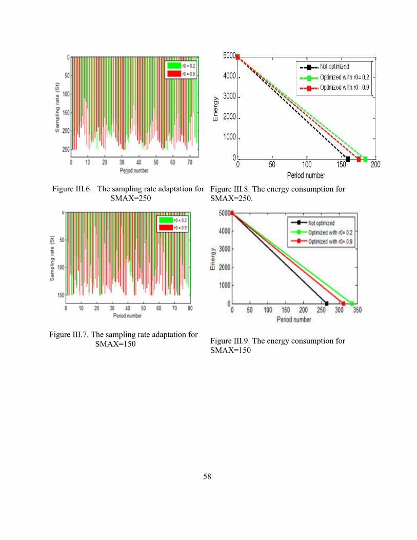
58
Figure III.6. The sampling rate adaptation for
SMAX=250
Figure III.7. The sampling rate adaptation for
SMAX=150
Figure III.8. The energy consumption for
SMAX=250.
Figure III.9. The energy consumption for
SMAX=150

59
VI. CONCLUSION
We provided an adaptive sampling approach for energy efficient periodic data
collection in sensor networks. We described two main mechanisms that form the core of
our approach. First we study the sensed data between periods based on the dependence of
conditional variance on measurements varies over time. Then, we proposed a multiple
levels activity model that uses behavior functions modeled by modified Bezier curves to
define application classes and allow each node to compute its sampling rate. We showed
that our approach can be effectively used to increase the sensor network lifetime, while
still keeping the quality of the collected data high.

60
Chapter IV Energy Efficient 2 tiers in-Sensor weighted data
aggregation
Exploiting sensors data should respect the characteristics of sensor networks in
terms of energy and computation constraints, network dynamics, and faults. Reducing
packet size transmitted and preparing the data for an efficient and scalable data mining is
very crucial. Such approach, leads us to think of a periodic data aggregation as a
preprocessing phase to achieve this goal. This chapter introduces a tree-based bi-level
periodic data aggregation approach implemented on both the source node and the
aggregator levels. Our contribution in this chapter is two folds. First we look on a
periodic basis at each data measured. Secondly, we clean it periodically while conserving
the number of occurrences of each measure captured. Then, data aggregation is
performed between groups of nodes on the level of the aggregator. The quality of the
information should be preserved during the in-network transmission through the number
of occurrence of each measure called weight. The experimental results show the
effectiveness of this technique in terms of energy efficiency and quality of the
information.
I. INTRODUCTION
The need of unattended operations in remote or hostile locations became an
eminent demand nowadays. Information collection and prediction for controlling and
predicting natural disasters, preventing failures, improving food production, and
improving human well-being are intended to wireless sensor networks. However as
presented in chapter II, sensor nodes are not expected to carry huge amount of data or
complex computations due to their presented constraints. It is important to remind that a
sensor network usually consists of thousands or ten thousands of nodes deployed
redundantly in order to ensure reliability. Subsequently, the collected data is partially

61
redundant and is subject to aggregation offering. In this context, data aggregation
constitutes energy efficient data management technique for wireless sensor network.
Furthermore, data accuracy is another main design concern in wireless sensor networks.
The distributed measurements nodes communicate wirelessly to a central gateway,
providing “interaction between people or computers and surrounding environment” [51].
To achieve data accuracy we strongly believe that only the right information should be
communicated through the wireless sensor networks. Intrigued by such interest, this
chapter suggests a periodic multilevel data aggregation algorithm aiming to optimize the
volume of data transmitted thus saving energy consumption and reducing bandwidth on
the network level. Instead of sending each sensor node’s raw data to a base station, the
data is cleaned periodically at the first level of the sensor node then another “data
aggregator “ sensor node collects the information from its associated nodes. We shall call
this the first level “in-sensor process periodic aggregation” approach. At the second level,
a heuristic data aggregation technique is applied on the level of the aggregator node
itself. This technique preserves the quality of the information through the number of
occurrences of each measure in the set called weight. The described approach focuses on
a periodical data aggregation while taking into consideration the weight of the data
captured. The output is a cleaned training set of data. This phase will constitute the
preprocessing step to get the perfect data set to be mined in an acceptable timeframe.
This will allow an optimization of the data mining algorithms that will be discussed in
chapter VI.
The rest of this chapter is organized as follows: the first section presents the
different data aggregation taxonomies and accredits data aggregation related work and
research. While the second introduces our data aggregation architecture scheme: the first
level periodic data aggregation algorithm applied on the sensor node level. At the second
level, a heuristic method aiming to aggregate data on the aggregator level and index the
data by a weight significant of its redundancy and quality. The Third section shows the
experimental results of our suggested bi-level aggregation algorithm and its contribution
to the network life in terms of energy consumption optimization. We conclude by
emphasizing the added value of our periodic data aggregation approach and its
contribution to the world of wireless sensor network research.

62
II. TAXONOMIES IN DATA AGGREGATION
Data aggregation in wireless sensor networks has been well studied in recent years
[52][53]. Data transmission is the most costly operation in sensors [54], compared with
it, the energy cost of in-network computation is sometimes trivial and negligible. In
consequences, the main challenge is the optimization of the energy consumed during the
transmission of the data. Computing and transmitting partially aggregated data to the end
user instead of sending the raw data will reduce the number of packets in the network
which save the energy of the sensor nodes [55]. Data aggregation techniques consist of
exploring how the data is to be routed in the network as well as the processing method
that are applied on the packets received by node. There are vast amount of extant works
on in-network data aggregation in the literature. Figure IV.1 illustrates the different data
aggregation schema existing in the WSN world. Actually, various structured and
unstructured algorithmic techniques have been proposed to allow efficient aggregation
without increasing the message size [62].
Figure IV.1 WSN Taxonomies
Four different topologies illustrated in Figure IV.1 can constitute the structured data
aggregation world: flat network, clustered network, tree based network and chain/grid
network.
Data Aggregation
Scheme
Structured
Flat Network
Clustered Network
Tree Based Network
Chain/Grid network
Unstructured Free scheme

63
A. Flat Network
Flat network based is a network composed of sensor nodes equipped with same
battery power and belonging to the same broadcast area. Figure IV.2 shows a
representation of a flat network. Some of the methods reported recently in such type of
network are query based methods [63] [64]. A query is generated at the sink and then
broadcasted through the network via multi-hop routes by using peer nodes as relays.
Some nodes just process the query, while others propagate it, receive partial results,
aggregate results, and send them back to the sink. A query is generated at the sink and
then broadcasted through the network. All protocols respecting this topology use a
technique that rely on a given node to broadcast received data and control packets to the
rest of the nodes in the network. This technique is called flooding and aims to find a
good-quality route from sources nodes to sink nodes. The main problem in this technique
is the implosion and overlap during routing since it doesn’t take into account the energy
constraint. Neighbors may also receive duplicate packets when two sensors sense the
same region and broadcast their sensed data at the same time. Different protocols exist in
this regard depending on the type of application aiming to restrict the flooding to
localized regions. Some examples of routing protocol based on flat topology are Sensor
Protocols for Information via Negotiation (SPIN) [52] [63], Directed-Diffusion[53],
Rumor-Routing[55],etc. The main advantages in the flat based topology are that no big
effort is needed to maintain and manage the network since non-complex switches or
routers are used. In addition, these protocols include a good quality routes from source to
sink. Unfortunately, flooding doesn’t respect the constraints imposed by sensor networks
since it is an expensive operation. To add also that the lifetime of a sensor network
decreases due to the unbalanced energy distribution and to the redundancy of packets
transmitted. High delay and unreliability also occur in such topology in case of large
network.

64
Figure IV.2 Flat Topology Architecture
B. Clustered Network
In a clustered network, the nodes are organized into clusters and a local
aggregator is introduced as a cluster head. The main function of a cluster head is to
aggregate data collected by all sensors existing in the same cluster before transmitting
them to the sink. This topology illustrated in figure IV.3 overcomes the constraint
imposed by large size network. It helps also in load balancing applications that require
scalability to thousands of nodes.
Some works, such as [65] [66] [67], use the clustering methods for aggregating
data packets in each cluster separately. Among these methods, the low-energy adaptive
clustering hierarchy (LEACH) protocol [68] [69] constitutes an example. LEACH
generates clusters based on the size of the sensor network. A drawback in this protocol
is the prior knowledge of the topology of the network. In [66], the authors propose a
self-organizing method for aggregating data based on the architecture CODA (Cluster-
based self-Organizing Data Aggregation). CODA relies on Kohonen Self-Organizing
Map to aggregate sensor data in cluster. Then clusters are combined or partitioned.
Before deployment, the nodes are trained to have the ability to classify the sensor data.
[66] proves that his method increases the quality of data and reduces data traffic as well
as conserves energy. An adaptive data aggregation (ADA) scheme for clustered sensor
networks has been also proposed in [67]. In this scheme, a time based as well as spatial
aggregation degrees are introduced. They are controlled by the reporting frequency at
sensor nodes and by the aggregation ratio at cluster heads (CHs) respectively. The
function of the ADA scheme is mainly performed at the sink node, with a little function
at CHs and sensor nodes.

65
At the end, all protocols adopting the clustered topology will have to choose a
cluster head, construct the cluster then transmit the data. The difference exists in the
implementation of these stages either through a fixed distribution or a dynamic one to
locate the sensor nodes and the cluster head.
The main advantage of a cluster based topology is the high scalability and the
optimization of energy consumption that extend the network lifetime. The channel
bandwidth is well utilized since the network is well organized. However we might face
cases were cluster heads are grouped on the same side of the network which lead to non-
uniform clustering. In consequences, no balanced energy distribution exists and energy
might be depleted to the long channel of communication between the cluster member
and the cluster head which lead to a decrease in the network lifetime.
.
C. Tree Based Network
In a tree based network, as illustrated in figure IV.4, a tree is constituted of sensor
nodes where data aggregation is performed at aggregators along the tree to arrive to the
sink. Tree based data aggregation approaches are suitable for in-network data
aggregation and aim to consume the lowest energy of the network. However, the
aggregation tree doesn’t share fairly the load of data packets to the transmitting nodes
which sometimes leads to heavily loaded nodes and results with the death of the
network. The authors in [70] [71], have proposed Tree on DAG (ToD) for data
aggregation, a semi structured approach that uses Dynamic Forwarding on an implicitly
constructed structure composed of multiple shortest path trees to support network
Sensor
Nodes
(SN)
Cluster
Heads
(CHs)
Base
Station
Figure IV.3 Cluster Based Topology architecture. Clusters boundaries referred by dotted line

66
scalability. The key principle behind ToD is the adjacent nodes in a graph which will
have low stretch in one of these trees in ToD thus resulting in early aggregation of
packets. An energy aware spanning tree (ESPAN) algorithm is proposed in [72] that
choose the node that has the highest residual energy as the root. Parent nodes are chosen
from neighbor nodes based on the residual energy and the distance to the root.
[73] proposes an energy-aware data aggregation tree (EADAT) algorithm. A
broadcast control message is sent periodically from the base station. A timer will start
on the level of each node once the message is received. When a node receives a
message, the timer is refreshed. The expiration time is inversely proportional to the
node’s residual energy. Therefore some nodes will be heavily loaded which will cause
depletion of energy and in consequences the death of the network. To overcome this
problem, [74] uses the genetic algorithm to calculate the possible routes represented by
the aggregation trees in order to balance the residual energy among the nodes. The
optimum tree is the adopted and the data load and the energy in the network are
balanced. This method can work only in case of homogeneous WSN with some spatial
correlation to monitor the environment. The most inconvenient point in this topology is
that the construction of the tree is time consuming and costly and if one parent node is
dead, the entire sub-tree is dead. The node in the leaf level are more likely to save
energy than the one closer to the base station that consume a lot of power when
forwarding packets received from the different nodes in the sub tree.
Figure IV.4 Tree based topology
D. Grid/Chain Based network
In a grid based data aggregation, the region to be monitored is divided into a grid.
Fixed regions of sensor networks contain a set of sensors assigned as data aggregators.
root
aggregator
sensor node

67
Sensors dispersed on the same grid transmit the data to the aggregators belonging to this
grid [75]. Communication is done only inside the grid and not among different grid like
the in network aggregation. The aggregator can be any node inside the grid on a round
basis till the death of the last node.
Some protocols such as PEGASIS [74] save energy dissipation of data transmission by
constructing transmission chain that connects the sensor nodes (figure IV.5). One of the
sensor nodes will lead the chain in a specific time-frame. Sensor nodes communicate by
choosing the closest node along the chain in direction of the leader till data is received
by the leader. The main objectives reached by PEGASIS are the enhancement of the
lifetime of each node through the collaborative technique, and the optimization of the
bandwidth consumed during communication.
Figure IV.5 Chain based topology
E. Structure free data aggregation
In a structure free data aggregation, no structure is adopted. Event driven models
are the typical example where we can adopt such structure since many changes are done
on the level of the event imposing several architectural reconstruction. However in a
structure free architecture, routing decisions need to be made on the fly. In addition, the
nodes ignore their upstream nodes and forward their own data without waiting to receive
data from other node. However, the positive side of this architecture, there is no need to
worry about the construction of the structure when some nodes fail. The first work done
on this point was by [68] where a MAC layer protocol for spatial convergence called
data-aware anycast (DAA) is proposed. DAA aggregates packets early on their route to

68
the sink. Then, another angle is tackled allowing some sensor nodes to wait for others
through a randomized waiting (RW) before sending data. It works as follow:
The node sends a “request to send” (RTS) packet with the type of data to its neighbor. In
his turn, the neighbor sends the “clear to send” (CTS) packet that have similar type of
data. After receiving the CTS from more than one neighbor, the source node selects only
one of them according to instantaneous channel condition. DAA is based on MAC layer
where in any casting we have the situation to select only one next hop among many. A
combination of the DAA and RW improves the performance in comparison with
structure approach.
F. Metrics for data aggregation in WSN
The efficiency of a data aggregation technique can be calculated using the below
different metrics:
1. The network lifetime prolongation that constitutes the target of any data
aggregation scheme since once all sensor nodes have died, the whole network is dead.
Efficient Energy consumption constitutes a main challenge for data aggregation as it
affects the network lifetime.
2. Minimizing latency which is very important since delay in data transmission may
consume more energy.
3. Enhancing data accuracy and avoiding data loss thus having better decision
making.
TableIV.1 shows a comparison between the different taxonomies of data aggregation in
a structure based topology taking into consideration the above metrics:
Advantages Drawbacks
Flat network Good quality routes from source to sink.
No topology maintenance overhead
Implosion problem due to duplicate
packets
Sink node might lead to the breakdown
of the entire network
High latency
Energy constraint not respected
Tree based Less power consumed
Optimization of energy
Unbalanced power consumption
between the closest nodes to the based
station and the nodes in the sub tree

69
Long delay for sending data from leaf
to root node.
Tree maintenance overhead is high.
Tree construction is time consuming
and costly.
Cluster based Enhanced scalability
Optimization of energy consumption
Efficient data aggregation that in
consequences lead to better utilization of the
channel bandwidth
The failure of a cluster head doesn’t affect
the whole network
Non uniform clustering leading to not
having cluster heads in some side of the
network
Failure of the sink node may
breakdown the entire network
Higher latency is involved in the data
transmission to the sink via multihop
Energy dissipation rate is highly
different from one sensor to another
sensor, even if they are in the same
cluster. Thus energy distribution is not
even.
Total energy dissipation increases due
to the long way communication between
a cluster member and cluster head.
Because of very long-way
communications, some sensors consume
energy rapidly and die. As a result,
network lifetime decreases.
Network connectivity may not be
guaranteed.
Chain Based Optimization in energy
Balancing in energy distribution
Prolongevity of the network lifetime
Too much delay for data collection.
High Topology management overhead
Table IV.1. Data Aggregation Taxonomies
In this chapter we will study a tree based data aggregation algorithm for periodic
sensor networks, where each sensor node takes measurements at regular time intervals
prior to send it to the aggregator. To the best of our knowledge, previous works didn’t
take into consideration the accuracy of the information affected by the number of
similarity between measures. Our aim is to periodically aggregate the data captured from
noisy and redundant measures while maintaining an acceptable level of quality and
accuracy of the information. The measures' occurrences are called weighted measures in
this chapter and will serve as a parameter passed to all data aggregation levels and
subsequently saving accuracy of the purged data. When applying the suggested
algorithm, it aggregates periodically the data while assigning to each measure its proper
weight. Such scheme will form an optimized training set for the classifier, predicting
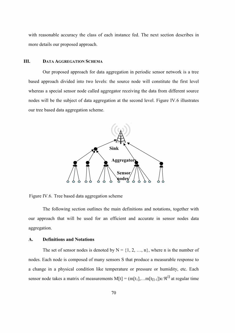
70
with reasonable accuracy the class of each instance fed. The next section describes in
more details our proposed approach.
III. DATA AGGREGATION SCHEMA
Our proposed approach for data aggregation in periodic sensor network is a tree
based approach divided into two levels: the source node will constitute the first level
whereas a special sensor node called aggregator receiving the data from different source
nodes will be the subject of data aggregation at the second level. Figure IV.6 illustrates
our tree based data aggregation scheme.
The following section outlines the main definitions and notations, together with
our approach that will be used for an efficient and accurate in sensor nodes data
aggregation.
A. Definitions and Notations
The set of sensor nodes is denoted by N = {1, 2, …, n}, where n is the number of
nodes. Each node is composed of many sensors S that produce a measurable response to
a change in a physical condition like temperature or pressure or humidity, etc. Each
sensor node takes a matrix of measurements M[t] = (m[t1],…m[t-1]) at regular time
Figure IV.6. Tree based data aggregation scheme
Sink
Aggregators
Sensor
nodes

71
interval t during a period . The unit time is called slot, whose length is the time interval
between two measurements. After -1 slot, each sensor node Ni will have a matrix of
measurements Mi as follows:
]1π[tsm........]2[tsm]1[tsm
]1π[t3m........]2[t3m]1[t3m
]1π[t2m.......]2[t2m]1[t2m
]1π[t1m.......]2[t1m]1[t1m
sM
3M2M1M
Definition IV.1: link between two measures
We define a link function link(m[ti], m[tj]), the degree of similarity between two
measures m[ti] and m[tj] collected at two slots i and j. This function returns either 0 or 1.
A higher similarity value indicates that the measures are more similar.
( [ ] [ ]) { [ ] [ ]
1)
Where is a threshold fixed by the application.
Definition IV.2: Weight of a measure
Intuitively, redundancy gives more importance to some information which, are
represented by many features and may occult less than others that are less present. We
define weight of a measure m at a time t the total number of measures captured after
the time t and can be similar to m.
i =Weight(m[ti]) = -1j=ti+1link(m[ti], m[tj]) (2)

72
Definition IV.3: Cell’s measure
On the level of an aggregator A, we define a cell of a measure Ca[i] = A[i](i,
mi), a cell that contains the received measure mi from the node ni with its corresponding
weight i. We refer to Ca[i](m) as the measure in a cell while the respective weight is
Ca[i]().
B. First Tier: Periodic data aggregation at the node’s level
At this level, our technique consists on evaluating the link function between two
measures taken at the same period before sending them to the aggregator. Hence, during
a period, when a node takes a new measure it calculates the link function with the
previous measure already captured during this period. If the link is equal to 1, this means
that the new measure can be aggregated with the existing measure on which we are
performing the link function. The weight of the existing measure is incremented by 1 and
the new measure is disregarded. For sake of simplicity and without loss of generality,
Algorithm IV.1 illustrates the first tier with one field of measure (i.e: temperature). At the
end of this algorithm, no redundant measures will exist. Each sensor will send to the
aggregator a set of reduced measures associated to their corresponding weight and ready
for the second tier data aggregation algorithm.
Algorithm IV.1: First Tier Data Aggregation
Input: New measure m[ti].
Output: Reduced set of measurements M.
Initialization: Get first measure m[t1]
1: 1 0
2: Foreach slot ti during a period do
3: Get a measure m[ti]
4: Foreach existing measure m[tj] do
5: If link (m[ti], m[tj]) = 1 then
6: j j+1 // j is the weight(m[tj])
7: Disregard [ ] 8: Else i i+1 //i is the weight(m[ti])

73
9: Add m[ti] to M: M {(M(i, m[ti])}
10: End if
11: End for
12: End For
C. Second Tier: weighted data aggregation at the aggregator level
At this level of aggregation, each aggregator has received k measures and their
frequencies. The idea here is to identify all pairs of measures whose similarities are
above a given threshold t. For this reason we use the same similarity function used at the
first tier. Thus we can treat pairs of measures with high similarity value as duplicates and
reduce the size of the final data set that will be sent to the sink.
Our approach aims at reducing data transmitted from the aggregators to the sink
subsequently reducing energy consumption. The obvious idea will suggest looping each
list comparing its measures with the remaining lists looking for redundant data. Such
approach proved to be costly in terms of data processing since it will scan the whole
existing set many times and is attributed a complexity of O(n!). Our approach, illustrated
in Algorithm IV.2, suggests building progressively a dynamic array list as follows:
We define A = Union of all existing lists in the aggregator: A = ((i,
m[ti])|iN). Then we select a random measure with its related weight from A in order to
create the first cell of our dynamic array list by placing the above random value in it. We
continue by selecting value (i, mi) from A and calculating the link function for each
selected value mi with the array list values { (j, mj), jarray list values}. The first
measure mj answering link (mi, mj) = 1 is observed and the weight of matched values are
added. If no match occurs the value is added to the dynamic array list by creating a new
cell. Finally, the selected value mi is deleted from A. As we proceed in the algorithm an
array list is built up.
Algorithm IV.2: Second Tier Data Cleaning
Input:
N: number of nodes associated to one aggregator A.
K: number of measurements received by the aggregator A.

74
A= (nk,m| nN, kK)= {(nk, mnk)| nN, kK} = {(11, m11),(12, m12) ,..,
(21, m21), …., (nk, mnk)}.
Output: Final dataset sent to the sink.
Initialization: We create a cell Ca[1] which contain a random value from the set
A.
1: L K
2: T 1 //T is the number of cells created
3: For i 2 to L do
4: Remove False
5: For j=1 to T do
6: Compute link(Ca[j](m),A[i](m))
7: If link(Ca[j](m),A[i](m)) =1 Then
8: Ca[j]() Ca[j]()+ A[i]()
9: Remove A[i](, m) from the set A
10: Remove True
11: End if
12: End For
13: If remove False Then
14: Build a cell Ca[j+1] to contain A[i](, m)
15: Remove A[i](, m) from A
16: Remove True
17: End if
18: L length (A)
19: T number of cells created for an aggregator.
20: End For
21: Built Array list of measures and weights.
1. Illustrative Example:
Let AM be the set of values related to one type of measures received from
different nodes connected to an aggregator A.

75
AM = {(11, m11),(12, m12), .., (21, m21), …., (nk, mnk)}.
We create the first cell Ca[1] in the array list where the first value (11, m11) collected is
placed. For each (ij,mij)we compute link (Ca[1](m), mij) where m is a measure from AM.
If the function returns 1 it means that these two measures are similar. Then the weights
are added to each other and we remove (ij, mij) from the set A, else we create a cell
Ca[2] for mij affected of the weight ij as shown in Table IV.1. for (12, m12) . At the end
we remove (ij, mij) from the set A.
Cells Ca[1] Ca[2]
11,m11 12, m12
Table IV.2. Array List under creation.
Supposing we are in the case where the measures are not similar we continue as follows:
We move to (13, m13), then we check if the similarity is reached with the measure m. If
so, the weights are added as follows: Ca[1]() = Ca[1]() + 13 and m=m13 is removed
from the set A. Otherwise we continue checking the similarity with the measure existing
in the second cell. If link (Ca[2](m), m13) =1 then Ca[2]() = Ca[2]() + 13 and m13 is
removed from the set A. If the measure is not similar with any of the existing measure in
the array we create a cell Ca[3] for m13 affected by its weight 13 before we remove (13,
m13) from the set A. Instead of looping through the entire set of values in A, we are only
scanning the cells progressively created in the dynamic array list while computing the
link function and reducing the original set size. If the latter is not verified then we create
a new cell containing the measure with its related weight otherwise we are only adding
the weight to an existing slot as in Table IV.2.
Cells Ca[1] Ca[2]
Weight 11, m11 (12+13),m12
Table IV.3. Sample of the Result Set sent to the aggregator

76
IV. EXPERIMENTAL RESULTS
To validate the approach presented in this chapter, we developed a C# based
simulator that we ran on the same readings collected from 46 sensors deployed in the
Intel Berkeley Research Lab [47] mentioned in chapter III. Every 31 seconds, sensors
with weather boards were collecting humidity, temperature, light and voltage values. In
our experiments, we are interested in two sensors measurements: the temperature and the
humidity. Each node reads an average of 83000 values of each measurement per day and
per field. All the results presented below are the average of 25 runs.
Output of our two tiers aggregation approach is presented below and include: (1)
output of first tier where the aggregation is done on a periodic basis every 31 seconds
(2) output of the second tier where the aggregation is done on the level of the aggregator
that receives the input from a group of nodes.
A. First tier: periodic data aggregation at the node’s level
At the first tier, data is filtered on a periodic basis where each period is
constituted of 31 seconds. At each period, each measure is affected by its weight. In these
series of simulations, we computed the percentage of the measurements sent by the nodes
to the aggregators after local aggregation. We varied the threshold delta between 0.01
and 0.07 based on the variation of measurements. Figure IV.9 shows the percentage of
data sent to the aggregator. Obviously the data size is disproportional to the threshold
data. The goal of this tier is to reduce the size of the data collected by each node while
preserving the frequency of each value as to not affect the analysis on the sink level. The
experimental results show that a minimum of 5% of the total set for each type of measure
is sent. The size of the affected weight for each measure is equal to the number of items
existing in the message to be sent to the aggregator. The total size of the messages sent to
the aggregator is then equal to the total number of measures to be sent in addition to the
total number of affected weight. As per the experimental results displayed in figure IV.7,
minimum of 10% for each measure is sent to the aggregator.

77
Figure IV.7. Percentage of total data sent to the aggregator
B. Second tier: weighted data aggregation at the aggregator’s level
At this level, weighted data measures are received by the aggregator. Weighted
data aggregation between all measures is performed at the level of the aggregator. It takes
as input the measures with their weight and gives as output one reduced set. This set
contains the aggregated measures associated to their weight. The weight of each measure
can define the number of occurrence of the data measure existing in this aggregator.
Results in Figure IV.8 show that maximum 13% of the data is sent to the sink adding to it
13% related to their respective number of occurrence. We conclude that only 26% of the
size of messages received by each aggregator A will be the aggregated data generated by
algorithm IV.2.

78
Figure IV.8 Second Tier Data Aggregation
C. Energy study
Sensor nodes used to form a sensor network are normally operated by a small
battery which has small amount of energy. Therefore, in wireless sensor networks
reducing energy consumption of each sensor node is one of the prominent issues to
address in the network lifetime. Since wireless communications consume significant
amount of battery power, sensor nodes should be energy efficient in transmitting data.
Protocols can reduce transmitted power in two ways. First where nodes can emit to short
distances such as data sinks or cluster nodes. The cluster node can then send the data
over a larger distance preserving the power of the smaller nodes. The second is by
reducing the number of bits (amount of data) sent across the wireless network. Our
approach reduces the overhead by detecting and aggregating redundant measures while
preserving the information integrity. To evaluate the energy consumption of our
approach we used the same radio model as discussed in [79]. In this model, a radio
dissipates Eelec = 50 nJ/bit to run the transmitter or receiver circuitry and βamp = 100
pj/bit/m2 for the transmitter amplifier. The radios have power control and can expand
the minimum required energy to reach the intended recipients as well as they can be
turned off to avoid receiving unintended transmissions. The equations used to calculate

79
transmission costs and receiving costs for a k-bit messages and a distance d are
respectively shown below in (3) and (4):
delecampd (3)
R delec (4)
Receiving is also a high cost operation, therefore, the number of receptions and
transmissions should be minimal. In our simulations, we used a measure length k of 64
bits which, corresponds to a packet length. With these radio parameters, when d2 is 500
m2, the energy spent in the amplifier part is equal to the energy spent in the electronics
part, and therefore, the cost to transmit a packet will be twice the cost to receive.
At the first level, and at the end of the period, each node will contain m messages
affected each by a weight . The size of the message sent by each node is equal to the
number of weight sent in addition to the number of values sent. We consider that each
value is equal to 64 bits. The total energy consumed is equal to the sum of the energy
consumed by each node when the packet is sent to the aggregator from the source nodes
and can be calculated as follows:
aggdxdxelecβampdelec
At the second level, the energy consumption will be equal to the energy consumed when
the aggregator send the data to the sink in addition to the energy consumed by the sink
when receiving the data as shown in (6).
sink d TxdRx elec βampd
elec
The total energy consumed on the level of the network is calculated as follows:
aggdsinkd
To evaluate the energy consumption of our approach we compared it to a classical
clustering approach, where every node sends all its measures to a cluster head which, in
his turn relays all the received data to the sink. Figure IV.9 shows that our approach

80
outperforms clustering approaches and minimizes the energy consumption by at least
50%.
Our approach is efficient since the information integrity is fully preserved. All
taken measurements appearing in the final set arrived to the sink along with their weight.
Therefore, we can consider that our approach decreases the amount of redundant data
forwarded to the sink and performs an overall lossless process in terms of information
and integrity by conserving the weight of each measure.
Figure IV.9. Energy Consumption
V. CONCLUSION
Data aggregation is a well-known technique to achieve energy efficiency, in
wireless sensor networks, when propagating data from sensor nodes to the sink. The
objective is rather than sending all captured data from sensors to the sink, multiple
redundant data are aggregated as they are forwarded by the sensor network. We
provided a two levels data aggregation scheme. At the first level we provided an
aggregator for simple captured measurements based on a link similarity function while
at the second one our objective was to detect and aggregate multiple data sets generated

81
by different neighboring nodes. It was shown through simulations on real data
measurements that our method reduces drastically the redundant sensor measures. In the
next chapter, another approach will be presented at the second tier relying on the sets
similarity in sensor networks.

82
Chapter V Data Aggregation in periodic sensor networks using sets
similarity
This chapter objective is to propose a new data aggregation approach aiming to
identify near duplicate nodes that generate similar sets of collected data in periodic
applications. We propose a new prefix filtering approach that avoids computing
similarity values for all possible pairs of sets. We define a new filtering technique based
on the quality of information. To the best of our knowledge, the proposed algorithm is a
pioneer in using “sets similarity functions” for data aggregation in sensor networks. To
evaluate the performance of the proposed method, experiments on real sensor data have
been conducted. The analysis and the results show the effectiveness of our method
dedicated to period sensor networks.
I. INTRODUCTION
An important topic addressed by the sensor networks community over the last
several years has been in-network aggregation. The idea is that cumulate time intervals,
or summaries can be computed directly within the network by sensor nodes, endowed
with computational power, thus avoiding the expensive transmission of all sensor data to
the sink. Previous work studied the data aggregation as the computation of statistical
means and moments, as well as other cumulative quantities that summarize the data
obtained by the network. To some extent these concerns can be alleviated by providing
tools for filtered aggregation, where only a selected subset of nodes participate in the
aggregation, according to the values of some of their sensors, their geographic location,
etc.
In this chapter we are interested in exploring a new part of the filtering aggregation
problem, by focusing on identifying the similarity between sets of data generated by
neighboring nodes further to a local processing technique. As highlighted, one of the
issues accompanying the growth of sensed data in periodic sensor networks is the

83
existence of near duplicate sets of data. Our objective is to identify similarities between
near sensor nodes, and integrate their sensed data into one record while preserving
information integrity. A quantitative approach in identifying two similar sets of sensed
data is by using a similarity function. Such function measures the degree of similarity
between two sets and returns a value between 0 and 1. A higher similarity value indicates
that the sets are more similar, thus we can treat pairs of sets with high similarity values as
duplicates, and send only one set to the sink instead of sending both. Similarity functions
were used in various domains and applications in order to identify near duplicate objects
(data). For instance, for Web search engines [53], Web mining applications [54],
detecting plagiarism [55], collaborative filtering in data mining [56], etc.
We provide a new prefix filtering method to study the sets similarity in sensor
networks. We propose frequency filtering optimization techniques, which exploits the
ordering of measurements according to their frequencies. A frequency of a measure is
defined by the number of occurrences of this measure in the set defined at the first
aggregation level. Furthermore, we provide a new optimization method for early
termination of sets similarity computing.
Our method is divided into two phases: the first one is done at the nodes level, where
each node compacts its measurements set according to a link function. The second is
defined at the aggregator level where the frequency filtering technique will be applied.
To evaluate our approach we conducted extensive experimental study using real data
measurements and we compare our approach to the existing ToD protocol [70, 71] for
data aggregation in sensor networks. The obtained results compared to the existing
algorithms show the effectiveness of our method which significantly reduces the number
of duplicate data.
The rest of this chapter is organized as follows: The first section gives an overview
on related works reported on the similarity between objects or records.. The second
introduces our data aggregation tree architecture scheme: the first level periodic data
aggregation algorithm applied on the sensor node level. At the second level, a heuristic
method based on the frequency ordering is proposed. Two optimization techniques based
on frequency filtering extension aiming to find similar data sets efficiently are presented.
The Third section shows the experimental results of our suggested data aggregation
algorithm and its contribution to the network life through optimizing energy

84
consumption. We conclude by emphasizing the added value of our approach and its
contribution to the world of wireless sensor network research.
II. PREVIOUS WORK
In this chapter we will follow the same hierarchical multilevel data aggregation
scheme presented in chapter IV aiming to optimize the volume of data transmitted thus
saving energy consumption and reducing bandwidth on the network level.
We are not aware of previous work that specifically addresses the set joins similarity
aggregation problem in sensor networks. Recently, many studies have proposed new
algorithms that define the similarity between objects or records. These algorithms are
classified into three categories, inverted index based methods [82], prefix filtering
methods [65], and signature based methods [83]. The most of these methods seem to be
pretty complex for wireless sensor networks usually generating large amount of
candidate pairs, all of which need to be verified by the similarity function. [87] applied
the Euclidean distance and cosine distance to reduce the packet size and minimize the
data redundancy of cluster-based underwater wireless sensor networks.
III. DATA AGGREGATION – OUR APPROACH
In this section we present our approach for data aggregation in sensor networks.
We consider the same tree based network adopted in previous chapter, where sensed data
needs to be aggregated on the way to their final destination. Sensor nodes collect
information from the region of interest and send it to aggregators. The aggregators can
either be special (more powerful) nodes or regular sensors nodes, or mobile agents like
robots that traverse the region of interest and collect the data sets. Each aggregator then
condenses the data prior to sending it. Our data aggregation method works in two phases,
the first one at the nodes level, which we call local aggregation and the second at the
aggregators’ level. At each period p each node sends its aggregated data set to its proper
aggregator which subsequently aggregates all data sets coming from different sensor
nodes and sends them to the sink.

85
A. Local aggregation
In periodic sensor networks, we consider that each sensor node i at each slot s takes a
new measurement yis . Then node i forms a new set of captured measurements Mi with
period p, and sends it to the aggregator. It is likely that a sensor node takes the same (or
very similar) measurements several times especially when s is too short. In this phase of
aggregation, we are interested in identifying locally duplicate data measurements in order
to reduce the size of the set Mi . Therefore, to identify the similarity between two
measures, we provide the two following definitions:
Definition V.1: link function
We define the link function between two measurements as:
{
(
1)
Where is a threshold fixed by the application.
Definition V.2: Measure’s frequency
The frequency of a measurement yis is defined as the number of the subsequent
occurrence of the same or similar (according to the link function) measurements in the
same set. It is represented by f (yis ).
Using the notations defined above we present the local aggregation algorithm
which is run by the nodes themselves (see Algorithm V.1). For each new sensed
measurement (at each slot), a sensor node i searches for similarities of the new taken
value. If a similar measurement is found, it deletes the new one while incrementing the
corresponding frequency by 1.
Algorithm V.1: Aggregation at the nodes level.
Require: New measure yisk , set of previous measures Mi .
Ensure: searching for similarities in Mi .

86
1: for every measure yisl ∈ Mi do
2: if (linkis (yisk , yisl ) = 1 then
3: f (yisl ) ← f (yisl ) + 1
4: delete yisk
5: else
6: add yisk to the set Mi
7: f (yisk ) ← 1
8: end if
9: end for
At the end of the period p, each node i possesses a local aggregated set Mi. The
second step is to send it to the aggregator which in his turn aggregates the data sets
coming from different sensor nodes.
B. Aggregation using similarity functions
At this level of aggregation, each aggregator has received k sets of measurements
and their frequencies. The idea here is to identify all pairs of sets whose similarities are
above a given threshold t. For this reason we use a similarity function which measures
the degree of similarity between the two sets and returns a value in [0, 1]. A higher
similarity value indicates that the sets are more similar. Thus we can treat pairs of sets
with high similarity value as duplicates and reduce the size of the final data set that will
be sent to the sink.
I. Similarity Functions
A variety of similarity functions have been used in the literature such as overlap
threshold, Jaccard similarity and Cosine similarity [84–86]. We denote |Mi | as the
number of elements (measures) in the set Mi . The following functions can be used to
measure the similarity between two sets of measurements Mi and Mj :
Overlap similarity: O(Mi , Mj ) = |Mi ∩ Mj |
Jaccard similarity:

87
Cosine similarity: √ Dice similarity:
All these functions are commutative and can be transformed to the Overlap
similarity easily. For instance, we can present the Jaccard similarity function as follows:
In our approach, we will focus on the Jaccard similarity. It is one of the most widely
accepted functions because it can support many other similarity functions [85]. In our
application, two given sets Mi and Mj are considered similar if and only if: where t is a threshold given by the application itself. This equation can be
transformed as: ⇔ (1)
where
In order to study the similarity functions for data aggregation in sensor networks, we
define a new function for overlapping ”∩s ” between two sets of measurements as
follows:
Definition V.3: Overlap function
Consider two sets of measurements M1 and M2, then we define:
M1 ∩s M2 = {(y1, y2 ) ∈ M1 × M2 / link(y1, y2 ) = 1}; and Os (M1 , M2 ) =
|M1∩sM2|.
For instance, we consider the following example:
Example1:
Consider 2 sets of measurements: { } { }

88
Such that:
M1 ∩s M2 = { } ⇒
To evaluate the similarity between two sets we obtain:
⇔ (2)
II. Sets similarity computation
In this section we provide techniques for computing the similarity between the
received sets. A naïve solution to find all similar sets is to enumerate and compare every
pair of sets as shown in algorithm V.2. This method is obviously prohibitively expensive
for large data sets (such the case of sensor networks), as total number of comparison is
O(n2).
Algorithm V.3: Naïve method for similarity computation.
Require: Set of measures’ sets M = {M1, M2 ...Mn }, and a threshold t.
Ensure: All pairs of sets (Mi , Mj ), such that J (Mi, Mj ) ≥ t.
1: S ← ∅ 2: for i=2 to n do
3: for j=1 to i-1 do
4: if Os (Mi, Mj) ≥ α then
5: (S { } 6: End if
7: End for
8: End for
9: Return S
To reduce the number of comparisons between sets, a prefix filtering method has
been proposed. Several approaches for traditional similarity join between sets are based
on the prefix filtering principle [84] [86] [9]. This method is based on the intuition that if

89
all sets of measures are sorted by a global ordering, some fragments of them must share
several common tokens with each other in order to meet the threshold similarity. An
inverted index maps a given measurement m to a list of identifiers of sets that contain mi
such that link(mi , m) = 1. After inverted indices for all measures in the set are built, we
can scan each one, probe the indices using every measure in the set M, and obtain a set of
candidates; merging these candidates together gives us their actual overlap with the
current set M; final results can be extracted by removing sets whose overlap with M is
less than [ (Equation 1).
This intuition is formalized by the following Lemma inspired from [86]:
Lemma V.1: Consider two sets of sensor measures Mi and Mj, such that their elements are
ordered by a global defined ordering. Let the p-prefix be the first p elements of Mi. If |Mi
∩s Mj | ≥ α, then the (|Mi |−α +1)-prefix of Mi and the (|Mj |−α +1)-prefix of Mj
must share at least one element.
Proof: Lemma V.1 can be proven similarly to the lemma of page 6 in [86].
To ensure the prefix filtering based approach does not miss any similarity set result,
as shown in Lemma V.1 we need a prefix of length |Mi | − t.|Mi | + 1 for every set
Mi [9]. The algorithm for finding similarity sets based on prefix filtering technique is
given in Algorithm V.3. It takes as input a collection of datasets coming from different
sensor nodes already sorted according to a defined ordering. It scans sequentially each set
Mi, selects the candidates that intersects with its prefix. Afterwards, Mi and all its
candidates will be verified against the Jaccard similarity threshold to finally return the set
of correct similar measurements sets.
Algorithm V.3: Prefix-filtering based algorithm.
Require: Set of measures’ sets M = {M1, M2 ...Mn }, and a threshold t.
Ensure: All pairs of sets (Mi, Mj ), such that J (Mi , Mj ) ≥ t.
1: S ← ∅ 2: Ii ← ∅ (1 ≤ i ≤ total number of measures)

90
3: for each set Mi ∈ M do
4: p ← |Mi | − t × |Mi | + 1
5: X ← empty map from set id to int
6: for k ← 1 to p do
7: w ← Mi [k]
8: if (Iws exists such that link(w, ws ) = 1) then
9: for each Measurement (Mj [l]), f (Mj [l]) ∈ Iws do
10: X [Mj ] ← X [Mj ] + 1
11: end for
12: Iws ← Iws {Mi }
13: else
14: create Iw
15: Iw ← Iw {Mi }
16: end if
17: end for
18: for each Mj such that X [Mj ] > 0 do
19: if Os (Mi , Mj ) ≥ α then
20: (S ← {(Mi , Mj )})
21: end if
22: end for
23: end for
24: return S
Prefix filtering algorithm helps prune out unfeasible sets of measures, however, in
practice the number of non-similar sets surviving after this technique is still quadratic
growth [88]. Following the prefix filtering, many optimization methods [88] [89] were
proposed to prune out further the unfeasible non-similar sets. A trade-off of these prefix
filtering optimizations is that usually require more computational efforts which is
unsuitable by heavy resources sensor networks. In our approach, we provide some
optimizations for prefix filtering techniques based on measures frequency while taking
into account this trade-off.

91
III. Frequency filtering approach
In this section, we present our frequency filtering method based on prefix
extension. We begin by introducing some definitions and notations which will be the basis
of what follows. In periodic sensor networks, two data sets are similar if their
measurements overlap with each other, and especially the ones having higher frequencies
values.
Definition V.4: Ordering O
We define an ordering O which arranges the measurements of a given set by the
decreasing order of their frequencies.
For two similar measures such that ( ) , we denote ( ) ( ) the minimum value of the frequency of these
measures.
Definition V.5: Consider two sets of measures Mi and Mj , we define ∑ ( ) ∈
In this chapter, we consider that all sensor nodes operate with the same sampling
rate, and every node captures τ measures with each period p. Thus we can deduce that
for every received set Mi from node i we have: ∑ ∈ Using the Jaccard similarity function, two sets Mi and Mj are similar if and
only if:
Os (Mi, Mj ) ≥ α where (2)
Supposing that the sets were sent to the aggregators without applying the first
aggregation phase and without computing measures frequencies, thus we can observe
that:
|Mi | = |Mj | = τ and fs (Mi, Mj) = Os (Mi, Mj). (3)
Hence, from Equation (2) and Equation (3) we can deduce that:

92
Mi and Mj are similar iff: (4)
IV. Frequency filter principle
Lemma1 states that the prefixes of two sets of measures must share at least one
measure in order to satisfy the prefix filtering condition (P F C). Nevertheless, in sensor
networks this condition is easily satisfied. In this section, we will present an extension of
the prefix filtering technique making the P F C condition more difficult to be satisfied.
Lemma V.2:
Assume that all the measures in the sets Mi and Mj are ordered according to the global
ordering O. Let the p-pref ix be the first p elements of Mi: ∑ ∈
Proof:
We denote by p-Mi the prefix of the set Mi and r-Mi the set of reminder measures
where Mi = {p-Mi + r-Mi}. We have:
∑ ∈
In the second line we can omit the term fs (p-Mi , r-Mj ) because we have assumed
that it is negligible compared to the other terms in the equation. Indeed, if the two sets are

93
similar then the measures having highest frequencies must be in the prefix set and not in
the remainder, which means that the overlapping between the p-Mi and r-Mj is almost
empty. From the above equations and equation (4) (similarity condition) we can deduce:
∑ ∈ (5)
From the following equation:
∑ ∈ ∑ ∈ (6)
We obtain:
∑ ( ∈ ) (7)
The lemma is proved.
Algorithm V.2 describes our method to find similar sets of measures based on the
frequency filtering approach. It is a hybrid solution, where we integrate our frequency
condition presented in Lemma V.2 to the prefix filtering approach presented in
Algorithm V.1.
V. Jaccard similarity computation
Although filtering approaches reduce the number of comparisons between the
received sets of measures, the number of candidate sets surviving after this phase is still
non negligible. Furthermore, the computation of the Jaccard similarity between two
candidates’ sets can be very complex, especially when it comes to sensor networks
where measures’ sets can have ten hundreds or thousands elements. Therefore, to
continue filtering out further candidate sets we propose a new frequency filtering
constraint in the verification phase. By applying this, we can also reduce the overhead of
the Jaccard similarity computation.
Algorithm V.2: Frequency-filtering based algorithm.
Require: Set of measures’ sets M = {M1, M2 ...Mn }, t, τ .
Ensure: All pairs of sets (Mi, Mj ), such that J (Mi, Mj ) ≥ t.

94
1: Replace line 5 in Algorithm V.1 with
2: F s ← empty map from set id to int
3: sumF req ← 0
4: for k ← 1 to p do
5: sumF req ← sumF req + f (mk ∈ p-Mi )
6: end for
7: Replace line 10 in Algorithm 1 with
8: F s[Mj ] ← F s[Mj ] + fmin (Mi [k], Mj [l])
9: Replace line 18 in Algorithm V.1 with
10: for each Mj such that F s[Mj ] > sumF req − do
Assume that we want to compute the similarity between two sets Mi and Mj.
Then, these sets are similar if they satisfy the overlap condition . We also
assume that a measure m ∈ Mi divides Mi into two partitions: one partition containing all
the measures having frequencies higher than f (m) including m denoted by h-Mi and
the second l-Mi containing all the measures having frequencies less than f (m).
Similarly, we assume that any measure in Mj divides it in two partitions h-Mj and l-
Mj. The idea of dividing the sets is to find a measure where at this position a similarity
upper bound is estimated and checked against the similarity threshold. As soon as the
check fails we can stop the overlap computing early. This hypothesis is formalized by the
following lemma:
Lemma V.3:
Assume that |Mi | < |Mj | and all measures in Mi are ordered according to the
global ordering O. Mi and Mj are similar ⇒ for any m ∈ Mi dividing Mi into h-Mi
and l-Mi we have:
∑ ( ∈ )
Proof. Mi and Mj are similar

95
⇒ (8) ⇒ (9) ⇒ (10)
Then we have: ∑ ( ∈ ) ∑ ( ) (11) ∑ ( ∈ ) (12) ∑ ( ∈ ) (13)
From equations (10) and (13) we can deduce that:
∑ ( ∈ )
The lemma is proved.
The algorithm of overlap computation is given in Algorithm V.3
Algorithm V.3: Overlap Computation.
Require: Two sets of measures Mi and Mj, t, τ .
Ensure: Os (Mi, Mj ).
1: Os ← 0
2: Consider |Mi | < |Mj |
3: sumFreqH ← 0
4: sumFreql ← τ
5: Mj ← sort(Mj, |Mj |) Mj is sorted in increasing order of the measures
6: for k ← 0 to |Mi | do
7: sumFreql ← sumFreql − f (Mi[k])
8: Search similar of Mi [k] in Mj
9: find Mj [l]/link(Mi [k], Mj [l]) = 1
10: sumFreqH ← sumFreqH + fmin (Mi[k], Mj[l])

96
11: if sumFreqH ≥ sumFreql then
12: Os ← Os + 1
13: else
14: Return −∞
15: end if
16: end for
17: Return Os
In this algorithm, we used two kinds of measures ordering depending on the sets
sizes. The first one according to the global ordering O (Mi in the above algorithm) and the
second is sorted in increasing order of the measures to accelerate a measure search.
IV. EXPERIMENTAL RESULTS
To validate the approach presented in this chapter, we developed a custom C#
based simulator. The objective is to confirm that our prefix filtering technique (PFF) can
successfully achieve intended results for data aggregation in sensor networks with
random distribution of sensor nodes. We performed experiments on the same real sensor
data measurements used in previous chapter. We exploited data collected from 46 sensors
deployed in the Intel Berkeley Research lab. Mica2Dot sensors with weather boards
collected timestamped topology information, along with humidity, temperature, light and
voltage values once every 31 seconds. Data was collected using the TinyDB in-network
query processing system, built on the TinyOS platform. In our experiments, we used a
file that includes a log of about 2.3 million readings collected from these sensors.
Temperature is in degrees Celsius. Humidity is temperature corrected relative humidity,
ranging from 0-100%. Light is in Lux. Voltage is expressed in volts [47]. In our
experiments, we are interested in two sensors measurements: the temperature and the
humidity fields since the variation is more frequent than the light and the voltage. Each
node reads an average of 1600 measurements per day and per field. The sensor readings
are generated based on intervals. According the variation of measurements, we choose to

97
vary the threshold delta between 0.01 and 0.07. All the results presented below are the
average of 7 days readings.
A. Local aggregation
In these series of simulations, we computed the percentage of the measurements
sent by the nodes to the aggregators after local aggregation. The results are shown in
Figure V.1. We noted the number of the measurements sent by the nodes to the
aggregators after local aggregation. The size of the set contains also the values of the
frequencies of each measurement. We considered that the size of each frequency value is
equal to the size of a sensor reading. In one day, the 46 sensor nodes collect around 8.0E
+ 4 measurements by field. It is well noticed that the size of data improves strongly
depending on the threshold δ. It decreases when δ increases.
Figure V.1 Percentage of total data sent to the aggregator

98
B. Aggregation using PFF technique
In this section we show the impact of our frequency filtering technique on data
aggregation in sensor networks. As before, we calculated the percentage of aggregated
sets as well as the information integrity.
Figures V.2 to V.4 show the percentage of number of sets not sent to the sink depending
on similarity and link thresholds that vary between 0.8 to 0.9 and between 0.01 to 0.07
respectively. For instance, we noticed that the size of the data set sent to the aggregator is
reduced by around 30% in case of δ = 0.07 and t = 0.8. The obtained results validated by
real data measurements, show clearly the effectiveness of our filtering technique in
finding and eliminating redundancy and comparing between two sets of data.
Figure V.2 Percentage of deleted sets, δ= 0.01

99
Figure V.3 Percentage of deleted sets, δ= 0.05
Figure V.4 Percentage of deleted sets, δ= 0.07
C. Data accuracy
We evaluate the impact of data accuracy by calculating the total number of measurements
in sets not sent to the sink (the aggregation error). Figures V.5 to V.7 show the
percentage of measurements not received by the sink. These results demonstrate clearly
that our approach conserves the information integrity. Therefore, we can consider that our

100
approach decreases the amount of redundant data forwarded to the sink and performs an
overall lossless process. In summary, the results obtained from real data sets of sensor
reading were qualitatively similar to the one obtained from a random scheme of data
measurements.
Figure V.5 Percentage of lost measures, δ= 0.01
Figure V.6 Percentage of lost measures, δ= 0.05

101
Figure V.7 Percentage of lost measures, δ= 0.07
D. PFF vs ToD aggregation protocols
In these experiments we compare our approach (PFF) to the ToD protocol proposed
in [71, 90]. In ToD, the network is divided into square cells, where each cell can contain
a number of sensor nodes. Then these cells are grouped into clusters called F-clusters
(first cluster). All nodes in F-clusters send their data to F-aggregators (cluster heads).
This structure is called F-tree. A second clustering layer (s-clusters) is built. It must
interleave with F-clusters so it can cover adjacent cells in different F-clusters. In the ToD
approach, the authors present data as events while in our simulations these data are sensor
readings. Thus, we consider every new reading as an event-like [71].
As our real data sensor network consists of 46 nodes, we use ToD in a one
dimensional Network as explained in [91] and we only divide the network into two F-
cluster.
We evaluated the performance of the protocols using the following parameters: a)
the number of sensor measurements taken by all nodes during a period τ , and b) the
threshold of the Jaccard similarity function t. The threshold δ is fixed to 0.07. The
aggregation function used for the ToD protocol is the same used in our approach (PFF)
based on the link function (cf section III[A]). We employ four metrics in our simulations:

102
• The number of candidate sets generated after applying the prefix filtering
approach [92], the frequency filtering algorithms with optimizations (PFF) and
the final result (the real number of duplicate sets);
• Percentage of received measures: It represents how effective a protocol is in
aggregating data. It is the number of measures received by the sink over the
number of measures taken by all nodes;
• Data accuracy: represents the measures loss rate. It is an evaluation of measures
taken by the source nodes which was not received at the base station (sink). It is
defined also as the aggregation error;Overall energy dissipation: is the total energy
dissipation of the entire network. To evaluate the energy consumption of our
approach we used the same radio model as discussed in [93]. In this model, a
radio dissipates Eelec = 50 nJ/bit to run the transmitter or receiver circuitry and
βamp = 100 pj/bit/m2 for the transmitter amplifier. The radios have power control
and can expend the minimum required energy to reach the intended recipients as
well as they can be turned off to avoid receiving unintended transmissions. The
equations used to calculate transmission costs and receiving costs for a k-bit
messages and a distance d are respectively shown below in (3) and (4):
delecampd (3)
R delec (4)
E. Percentage of received measures and data accuracy
Figure V.8, V.9 show the percentage of received measures over the total number
taken by all nodes for the temperature field. These experiments permit to show how well
aggregation protocols do aggregation and reduce redundant measures. PFF performs
better than ToD in terms of data aggregation because of it is ability to compare sets of
data instead of single packets. In other words, PFF reduces the number of redundant data
traveling into the networks better than TOD especially when the number of readings
increases (the case of periodic networks). We also notice that, the percentage of received
packets remains almost unchangeable while increasing the sensor readings.

103
Figure V.10, V.11 depicts the results of the aggregation error for temperature and
humidity fields respectively. This metric is an important performance index, and the high
measures loss rate will impact the use of the data greatly. The obtained results show that
the two protocols have good performance regarding the aggregation error. As expected,
when we increase the threshold t of the similarity function we reduce the measures loss
rate. For instance, we can notice that PFF outperforms ToD in terms of data accuracy for
t = 0.9.
Figure V.8 Received Measure (Temperature)

104
Figure V.9 Received Measure (Humidity)
Figure V.10 Data accuracy (Temperature)

105
Figure V.11 Data accuracy (Humidity)
F. Overall energy dissipation
The overall energy dissipation is the total energy consumption of the entire
network. Figure V.12. shows the results for total energy consumption obtained while
varying the total number of sensor readings. The figure shows that the overall energy
dissipation for different protocols increases as the number of readings increases. We
notice that ToD consumesfairly, but does not scale well as the number of readings
increases. For all the values of the threshold t tested, PFF always outperforms the ToD
protocol in total energy dissipation. This is because, the packet-packet comparison used
in ToD instead of data sets in PFF generates more transmissions in the network, and
furthermore, the packet construction in ToD contains additional information required for
the aggregation which is not the case in PFF. To conclude, PFF uses a factor of 1.5 to 2.5
less overall energy than ToD as shown in Figure V.12.

106
Figure V.12 Total energy dissipation
V. CONCLUSION
Data aggregation is a well-known technique to achieve energy efficiency, in wireless
sensor networks, when propagating data from sensor nodes to the sink. The main idea
behind is that rather than sending all captured data from sensors to the sink, multiple
redundant data are aggregated as they are forwarded by the sensor network. In this
chapter, we proposed a new method based on sets similarity functions and prefix filtering
technique for data aggregation in periodic sensor networks. In periodic networks, nodes
are likely to send multiple correlated data to the sink, thus causing the propagation of
redundant information throughout the network which in turn leads to both a waste of
energy resources and bandwidth, and increase in network congestion. The objective of
our aggregation approach is to reduce the number of redundant data sent to the final user
while preserving the data integrity. We have developed a new frequency based prefix
filtering technique that avoids computing similarity values for all possible pairs of sets.

107
We used the Jaccard similarity function to estimate the similarity between sets of data
measures. It was shown through simulations on real data measurements that the proposed
method reduces drastically the redundant sensor measures while preserving information
integrity. Therefore, it saves energy and improves the overall network lifetime.

108
Chapter VI Data Mining in periodic sensor networks: K-Means
clustering
Tides of data captured by sensors networks represent a powerful resource for
mining. Data mining is a perfect tool to analyze, categorize data and summarize the
relationships identified. However, high computational cost imposed by data mining
techniques as well as limitation existing in sensor networks in terms of energy and power
constitute a major challenge.
At the same time, big data generated by periodic wireless sensor networks can’t
be easily mined. All of this has led to the development of new multilevel optimized
version of a data mining algorithm named « k-means ». In this chapter we present an
efficient prefix mining algorithm in periodic wireless sensor network, both from a
statistical and computational point of view.
Periodic preprocessing algorithm based on prefix filtering technique is applied on
big data generated by periodic sensor networks. Then a K-means optimization technique
in terms of comparison and number of iterations is applied by exploiting prefix subsets of
data. The main idea of this technique is to optimize the clustering of observations
generated by periodic sensor networks into groups of related readings without any prior
knowledge of the relationships between the prefixes sets. Simulations results are
presented to validate the performance of the proposed approach.
I. INTRODUCTION
During last years, the main deal of interest reside in applying recognized
unsuitability of traditional data warehousing and knowledge discovery methodologies
within the challenges posed by sensor networks. Too much data overwhelm the WSN and
effectively consume a lot of memory and power when transported. As already stated, it is
well known that communicating messages over a sensor network consume far more

109
energy than processing it. These constraints should be respected by any technique that
needs to be applied on the periodic sensor networks. It is therefore mandatory to user
request while avoid sending all the data across the network. Thus we introduce the value
of applying data mining algorithms on the sensor network.
With the rapidly increasing amount of data gathered over 3 years period, data
mining is becoming an increasingly important tool to transform such data into
information. Such mining practices are commonly used in a wide range of profiling
practices, including marketing, surveillance, fraud detection and scientific discovery.
Data mining is generally defined as the process of extracting patterns from data.
Data mining is often associated with analyzing large amounts of data, usually in
the form of centralized database table, for useful and interesting information. The current
limitation of data mining applications in sensor networks is that existing distributed data
mining techniques impose heavy demands on computation and/or communication.
Making data mining in sensor networks even more challenging by overcoming the
individual sensor constraints of available energy for transmission, computational power,
memory, and communications bandwidth undertaking efficiently the data mining process
on the sensor network. Centralized data mining in sensor network and distributed data
mining in sensor network are two interesting research fields. We summarize the
advantages and the differences between the two approaches. The simplest approach is the
use of a centralized architecture where a central server maintains a database of readings
from all the sensors. The problem arises where the sensor networks is made of thousands
of node, the number of messages sent in the system as well as the number of variables of
the data mining task will be too large to be managed efficiently. A solution suggests the
introduction of intermediary nodes (aggregators) having the capability to fuse the
information from different sources before being transmitted along the network [94] [95].
On the other hand, heavy traffic over the limited bandwidth wireless channels will result
from central collection of data from every sensor node which will drain a lot of power
from the devices. A solution proposed by recent researches consist of a distributed data
mining (DDM) approach that pays careful attention to the distributed resources of data,
computing, and communication in order to consume them in a near optimal fashion. In
such, distributed clustering methods, each sensor collects a set of data (measures) and

110
aims to design local clustering rules that perform at least as well as global ones which
rely on all data being centrally available. However, transmitting the entire collected data
to a centralized location consumes a lot of energy. This suggests the development of “in-
network” clustering algorithms that only require exchanging information with one hop
cluster head or aggregator to solve the unsupervised classification problem in a fully
distributed manner. A popular iterative solution to the distributed clustering problem is
the k-means algorithm [110]. The algorithm alternates between two major steps
(assigning collected data to clusters and computing cluster centers) until a stopping
criterion is satisfied.
Our thinking consist of a hierarchical architecture for data mining in periodic
sensor network aiming to reduce the communication load and also reduce the battery
power more evenly across the different nodes in the sensor network by introducing a
preprocessing phase. In this chapter, our hierarchical data mining approach consists of
integrating the data aggregation phase presented in previous chapter as a preprocessing
step with the traditional k-means algorithm. We applied k-means on prefixes sets of
collected data instead of all data sets. Our suggested approach is folded in two steps: the
first one is the “pre-processing prefix frequency filtering technique” presented in chapter
V, which ensures similar sets of data generated by neighboring nodes. In order to reduce
the number of sets comparisons, for each set we compute a prefix subset based on its
length and the threshold of a well-defined similarity function. At the second step, we
exploit these prefixes to adapt a “k-means clustering, on the prefixes sets in order to
cluster observations into groups of related observations without any prior knowledge of
the relationships between the prefixes sets. Our main objective is to use solely subsets of
data instead of using the whole collected data in a clustering k-means algorithm. In this
chapter we design an efficient prefix mining algorithm in sensor network, both from a
statistical and computational point of view. On the other hand, we will be addressing the
energy problem in sensor network and the problem of mining big data generated sensor
networks by mining prefix set of periodic data.
The rest of this chapter is organized as follows: section II gives an overview of
related works reported on data mining and k-means clustering in sensor networks. We,
then briefly describe k-means algorithm. The problem statement and the mining of prefix

111
item sets resulted from chapter V are also presented in this section. Simulation results are
given in Section IV. Section V concludes the chapter.
II. RELATED RESEARCH
The deployment of data mining techniques in sensor networks is an open research
problem. This section will include two parts: first part will present the works and
limitations of applying the data mining techniques on a centralized architecture of WSN.
The second part will explore the work related to distributed data mining techniques in
WSN.
A. Centralized Approach: related research
Mining the large data repository generated by a sensor network for useful
information is crucial and challenging. The simplest approach to analyze sensor network
data makes use of a centralized architecture where a central server maintains a database
of readings from all the sensors. The limitation of this approach appears when the sensor
networks is made from thousands of nodes where the number of messages sent in the
system as well as the number of variables of the data mining task are too large to be
managed efficiently.
Another important issue is that routing may be based on data centric. Such
routing, the interest dissemination is performed to assign the sensing tasks to the sensor
nodes. The data aggregation is a technique used to solve the implosion and overlap
problems in data centric routing [79]. In this technique, a sensor network is usually
perceived as a reverse multicast tree where the sink asks the sensor nodes to report the
ambient condition of the phenomena. Data coming from multiple sensor nodes are
aggregated as if they are about the same attribute of the phenomenon when they reach the
same routing node on the way back to the sink. Data aggregation can be perceived as a
set of automated methods of combining the data that comes from many sensor nodes into
a set of meaningful information [79]. With this respect, data aggregation is known as data
fusion [79]. Also, care must be taken when aggregating data, because the specifics of the
data, e.g., the locations of reporting sensor nodes, should not be left out.

112
This solution, however, consumes too much energy because the data volume can
be extremely large. A good method should require little data transmission, but still
achieves information extraction from the large amount of data distributed across the
network. An alternative consists of aggregating systems where the data obtained from
different source nodes can be aggregated before being transmitted along the network
[101]. Intermediary nodes having capability to fuse the information from different
sources are integrated as aggregator in the system. [100] proposes a two layer topology of
a sensor network made of a lower level whose task is to organize the sensors in clusters,
compress their signals and transmit the aggregate information in the upper level playing
the role of a data mining server which uses the aggregate information to carry out the
required sensing task. The data mining architecture proposed the Lazy Learning
algorithm which is a supervised learning technique. [100] deems that this algorithm is a
promising tool in the sensor network context. This algorithm on a query-by-query basis,
tunes the number of neighbors using a local cross-validation criterion. In his paper, [100]
advocates the idea that the structure of the processing architecture of a sensor network
must take into account also criteria related to the accuracy and quality of the data mining
task. This means that the organization of the same sensor network may change according
to the type of sensing task (e.g. classification or prediction) and the required quality and
precision.
[58] considers a very important data mining problem: outlier detection, which
defines a process to identify data points that are very different from the rest of the data
based on a certain measure. In his paper, [104] consider the problem of finding two types
of distance-based outliers in sensor networks. He proposed to use a histogram method to
extract hints about the data distribution from the sensor network. The histogram
information can help filter out the non-outliers and identify the potential outliers within a
certain range. Those potential data ranges can be further refined with more histogram
information or identified by individual check. The histogram method reduces the
communication cost dramatically versus the centralized scheme. On the other hand, [116]
proposes in-network clustering algorithm to detect outlier values and classify them to
either noisy data or interesting event in the physical environment.

113
Other algorithms adopted for in-sensor-network has been developed within the
artificial neural-networks tradition [102] [117] where the application demands
compressed summaries of large spatio-temporal sensor data and similarity queries, such
as detecting correlations and finding similar patterns. Unsupervised learning Artificial
Neural Networks such as ART class algorithm typically perform dimensionality
reduction or pattern clustering. They are able to discover both regularities and
irregularities in the redundant input data by using an iterative process of adjusting
weights of interconnections between a large numbers of simple computational units
(called artificial neurons). As a result of the dimensionality reduction which is easily
obtained from the outputs of these algorithms, lower communication costs leading to
considerable energy savings can also be achieved. As a consequence of its stability-
plasticity property, the network is capable of learning “on-line”, i.e. refining its learned
categories in response to a stream of new input patterns, as opposed to being trained “off-
line” on a finite training set. Because of its computational advantages, complement
coding is used in nearly all ART applications. The strengths of the ART models include
its unique ability to solve a stability-plasticity dilemma, extremely short training times in
the fast-learning mode, and an incrementally growing number of clusters based on the
variations in the input data. The network runs entirely autonomously; it does not need any
outside control, it can learn and classify at the same time, provides fast access to match
results, and is designed to work with infinite stream of data. All these features make it an
excellent choice for application in wireless sensor networks. A neural network algorithm
can be implemented in the tiny platform of Smart-It units, which are kind of sensor nodes
or motes. Instead of reporting the raw-data, each Smart-It unit can send only the cluster
number where the current sensory input pattern has been classified. In that way a huge
dimensionality reduction can be achieved depending on the number of sensor inputs in
each unit. In the same time communication savings will benefit from the fact that the
cluster number is a small binary number unlike sensory readings which can be several
bytes long real numbers converted from the analog inputs. The uses of limited resources
together with the distributed nature of the sensor-networks has lead also to distributed
algorithmic solution for data clustering.

114
B. Distributed approach: Related Research
With their own processing power, the sensors become active devices allowing the
possibility to implement distributed algorithms in a network of sensors. One application
is the distributed stream mining system Vedas [97] by Kargupta et al., which monitors
data streams obtained in moving vehicles before reporting them to a base. More recently,
Banyopadhyay et al. [96] introduced a distributed clustering algorithm based on the k-
means clustering algorithm in a peer to peer environment. We briefly discuss classical K-
means clustering for readers not familiar with the problem.
K-means clustering: Simply put clustering, is the grouping of similar objects (data
points) in a way that minimizes intra-cluster dissimilarity while maximizing inter cluster
dissimilarity. K-means clustering is a classical clustering technique where K, the number
of clusters, is fixed a priori. The goal is to divide the objects into K clusters minimizing
the sum of the average distances to the centroids over all clusters. Finding an optimal
clustering is hard (NPcomplete), so the most common approach is to employ an iterative,
greedy search as described below:
1. Place K points randomly. These represent the initial cluster centroids.
2. Assign each point to the closest centroid.
3. Recalculate the positions of each centroid (the average of all data points
assigned).
4. Repeat Steps 2 and 3 until the centroids do not change. The assignment of
points to the final centroids forms the clustering.
Hence, [101] shows that distributed clustering algorithms based on artificial
neural networks, seem useful for mining sensor-network data or data steam. An exact
local algorithm for majority Voting which is always guaranteed to terminate with
precisely the same result that would have be found by a centralized algorithm, show how
it can be used as a primitive for monitoring a K-means clustering [106].
Although these algorithms achieve exact solutions eventually, they are limited to
problems which can be reduced to threshold predicates. For example it is very difficult
(perhaps impossible) to develop an exact local algorithm to compute the mean of a set of

115
numbers distributed over the network, but not so for evaluating whether the mean lies
above a threshold. In light of this, some data mining problems are very difficult, perhaps
impossible, to solve with exact local algorithms – in particular, K-means clustering.
Following this, an approximate local algorithm offering an approximate solution for
incrementally computing a K-means clustering has been developed in [113][114]. The
algorithm is initiated with a set of randomly chosen starting centroids distributed over all
peers. In each iteration, each peer runs a two-step process. The first step is identical to
one iteration of standard K-means where the peer assigns each of its own point to its
nearest of k cluster-centroids. In the second step, peer sends a poll message, consisting its
id and current iteration number to its immediate neighbors and waits for their responses.
Each response message from a neighboring peer contains the locally updated centroids
and cluster counts of that peer for the iteration.
[76] proposes a framework for building and deploying predictors in sensor
networks that pushes most of the work out to the sensors themselves. [76] Consider only
the hubbed sensor networks where the network structure is a tree. In this technique each
sensor may collect only a single attribute. A target class is associated with each global
reading; for training data, there is a further column containing these target classes. After
deployment, the goal is to predict the target class for each global reading. So at the end,
each sensor builds a local predictor that predicts the target class based only on the
attribute(s) available to it locally. At the root, local predictions are combined using
weighted or unweight voting. The network is a tree, with a powerful computation device
at the root, and sensors, with limited power, processing, and memory capabilities at the
leaves. The bandwidth in the network is a scarce resource, in part because transmission
by the sensors consumes power. In this overall approach, the variations depends on the
predictive technique being used either it required access to all of the training data at once
like decision tree or it requires only one reading at a time like neutral networks. In both
cases, sensors must have enough memory to store the model itself and to hold the entire
training data for its input attributes. [76] proves that the overall classification accuracy for
both the simple and the weighted voting scheme is a good or better than that of the
centralized data mining approach. In this approach each sensor learns a local predictive
model for the global target classes. Only the predicted target class for each reading is then

116
transmitted to the root, which determines the appropriate prediction by voting the target
classes of the local predictors. The prerequisite of this approach is that the target class
prediction should be predefined otherwise this approach is not valid.
Other research related to the distributed data mining introduced the collective data
mining[6] where the framework is constituted by the fact that the function to be learned
by the data mining algorithm, can be expressed as a sum of basic functions and their
corresponding coefficients. By using such technique, the sum is only approximated and
the computation is expensive on the sensor. Since it is approximate calculation, this puts
an upper boundary on the accuracy that can be achieved.
The existing distributed data mining techniques in sensor networks impose heavy
demands on computation and/or communication. We are not aware of previous work that
specifically addresses the prefix filtering to mine large item sets problem. Our idea is to
reduce the size of data to be mined without losing the main information through our
hierarchical approach.
III. PREFIX K-MEANS IN SENSOR NETWORKS
Data mining algorithms are designed for the relational data model. That is why
the existing works consider homogeneous schemata containing same set of attributes
across different sites. Typically the same algorithm operates on each distributed data site
concurrently, producing one local model per site. Subsequently all local models are
aggregated to produce the final model. The success of data mining algorithms lies in the
aggregation. Each local model represents locally coherent patterns, but lacks details that
may be required to induce globally meaningful knowledge. For this reason, many data
mining algorithms required a centralization of a subset of local data to compensate it.
Therefore, minimum data transfer is another key attribute of the successful data mining
algorithm. Our approach consists of considering each sensor as a data site. A feature
selection algorithm will first be applied on each data site resulting by minimizing the set
of attributes existing in each sensor and producing a local model per site. The main idea
of feature selection is to eliminate useless and redundant features. The learning process is
then accelerated and the accuracy of learning algorithms may be improved [110].

117
All the presented work didn’t take into consideration the accuracy of the
information affected by the number of similarity between measures. Our approach starts
with a preprocessing phase that uses the approach presented in chapter V.
In this chapter we shall focus on mining the prefix item sets resulted from the
preprocessing phase since such scheme will form an optimized training set for the
classifier, predicting with reasonable accuracy the class of each instance fed. However, in
data mining the task of finding frequent pattern(FP) in large databases is very important
but is computationally expensive, especially when a large number of patterns exist with
different set size of attribute. Han & al. [76] propose an FP growth algorithm which use
an extended prefix-tree structure for storing compressed and crucial information about
frequent patterns named frequent-pattern tree (FP_Tree). In his study, Han proved that his
method outperforms other popular methods for mining frequent patterns, e.g. the Apriori
Algorithm and the TreeProjection [77]. However the FP growth is expensive to build in
terms of CPU and time.
Our work considers a three level tree-based representative network. The first level
is the sensor node level where data captured and cleaned on a periodic basis then sent to
the aggregator. At the second level, each aggregator condenses the data sets based on
prefix frequency filtering technique [9], prior to apply our k-means prefix mining. Our
aim is to use the prefix of the frequent item sets collected from the first step as the
optimization key for the generation of frequent pattern based on the structure generated
on the level of the aggregators as shown in Figure.VI.3.

118
Figure.VI.1 K-Mining similar prefix sets in wsn
A. The k-Means algorithm:
Definition VI.1: K-means
Classifying or grouping data based on attributes/ features into k number of groups
is called k-means. k is a positive integer number based on which the number of clusters
are defined. The grouping is done by minimizing the sum of squares of distances between
data and the corresponding cluster centroid.
K Means recall
The main idea is to define k centroids, one for each cluster. These centroids
should be placed in a cunning way because of different location causes different result.
So, the better choice is to place them as much as possible far away from each other. The
next step is to take each point belonging to a given data set and associate it to the nearest
centroid. When no point is pending, the first step is completed and an early grouping is
done. At this point we need to re-calculate k new centroids as barycenter of the clusters
resulting from the previous step. After we have these k new centroids, a new binding has
to be applied between the same data set points and the nearest new centroid. A loop has
been generated. As a result of this loop we may notice that the k centroids change their
si
K- means K- means
Source
nodes
Aggregator Aggregator Frequency
Filtering Prefix Filtering
K-Means on the level of the super aggregator

119
location step by step until no more changes are done. In other words centroids do not
move any more.
The steps of the K-means algorithm are presented below.
K-means recall
1: Determine the centroid coordinate by placing K points into the space
represented by the objects that are being clustered. These points represent
initial group centroids.
2: Assign each object to the group that has the closest centroid according to
the minimum distance.
3: When all objects have been assigned, recalculate the positions of the K
centroids.
4: Iterate Steps 2 and 3 until the centroids no longer move. This produces a
separation of the objects into groups from which the metric to be
minimized can be calculated.
Although it can be proved that the procedure will always terminate, the k-means
algorithm does not necessarily find the most optimal configuration, corresponding to the
global objective function minimum. The algorithm is also significantly sensitive to the
initial randomly selected cluster centers. The k-means algorithm can be run multiple
times to reduce this effect. K-means is a simple algorithm that has been adapted to many
problem domains.
B. Our algorithm: The prefix set k-means technique
The existing work done in k-means doesn't take into consideration the
computational time in periodic sensor networks. Our aim is to respect the constraint
imposed by the sensor network and to minimize the computational time for online
clustering. The preprocessing phase based on the prefix filtering approach applied in
chapterV will output the all pairs of sets (Mi, Mj). This output will be taken as input in
our K-means algorithm.

120
Definitions and Notations
In this section we will introduce some definitions and notations that will be used
in our approach.
Definition VI.2: Measure’s frequency f The frequency of a measure is defined as the number of subsequent occurrence of
the same similar measurements in the same set.
Definition VI.3: Aggregator of Set AM
We define AM, aggregator of sets as the Union of all sets received by an
Aggregator such that for all similar measures between those sets we keep the sum of their
frequencies.
Definition VI.4: Means of Set
We define i
AM as means of a set i
M the average of measures existing in the set
Mi.
An
n
kk
m 1
iM such that n is the number of elements
Definition VI.5: General Similarity function
We will use as follows a generalization of the distance of Manhattan to check the
similarity between the pairs of set generated by each aggregator:
Definition VI.6: Average absolute deviation between pairs of sets:
The average absolute deviation function of pairs of sets is defined by the function
Sf as follows:
|f
mn
1ii
AM|n1Sf
|j
Mi
AM|j)d(i, A

121
such that
Definition VI.7: Standardization of pairs of sets
The standard function of sets i
AM is defined by the function if
z as follows:
In a nutshell, we generalize the prefix defined in our previous chapter by the
following lemma VI.1.
Lemma VI.1:
Consider two aggregators of sets of sensor measures AMi and AMj, such that
their elements are ordered by a global defined ordering. Let the p-prefix be the first p
elements of AMi. If |AMi ∩s AMj| ≥ α, then the (|AMi |−α +1)-prefix of AMi and
the (A|Mj |−α +1)-prefix of AMj must share at least one element.
Proof:
The Lemma can be proven similarly to the lemma1 in [8].
This method is based on the intuition that if all sets of measures are sorted by a
global ordering, some fragments of them must share several common behaviors with each
other in order to meet the threshold similarity and belong to the same cluster. Therefore,
the prefix will consist of the most reliable data since it is extracted based on global
frequency ordering. This leads us to think of working on the prefix set instead of the
whole set. An inverted index maps a given measurement to a list of identifiers of sets that
contains mi such that link (mi, m) = 1. After inverted indices for all measures in the set
are built, we can scan each one, probe the indices using every measure in the set M, and
obtain a set of candidates; Adapting K-Means on these candidates in order to group them
together in the same cluster gives us their actual overlap with the current set M; final
results can be extracted by clustering all sets. K-means will be adapted then to be
fs
fm
i
AM
if
z
.)|j
Mi
AM|n
1
fm A

122
applied on the similar prefix sets results of detecting and aggregating multiple data sets
generated by different neighboring nodes instead of applying it on the whole set of data.
C. K-means algorithm on the level of the super-aggregators:
Using the functions defined above we present a new technique of k-means applied
on the prefix pairs of sets preprocessed after applying prefix frequency filtering described
in Chapter V. This technique is run by one aggregator introduced on the top of all
aggregators (algorithm VI.1).
Similar sets are extracted based on the prefix frequency filtering already presented
in chapter V which will constitute the preprocessing step of the K means. AM is then
constructed on the level of each aggregator as per definition6 where frequency of the
similar sets are added to the non-similar sets. Each aggregator will then send AM to the
super-aggregator where the K-means is applied as per algorithm1. At the end of the k-
means clustering algorithm applied on the prefixes sets we have clustered similar sensor
node into groups of related sensed data. Sensor Nodes belonging to the same cluster
means that they will generate similar set of data. Using this hypothesis, the network life
cycle will be optimized by applying algorithmVI.1.
Algorithm VI.1: k- means on prefix pairs of set
Require: Set of measures’ sets AM = {AM1 , AM2 ...AMn }and a number of k random
centroids
1: Get prefix of all pairs of sets (AMi, AMj) results in different aggregator
as per LemmaVI.1.
2: Extract similar sets existing in AM based on the frequency filtering
algorithmVI.1
3: Standardization of pairs of sets by calculating ASf
4: Compute the minimum distance of Manhattan between the means of the
prefix pairs of sets.
5: Assign each prefix to the group that has the closest centroid according
to the minimum distance between the means.

123
6: When all objects have been assigned, recalculate the positions of the K
centroids.
7: Reiterate steps 5 and 6 until the centroids no longer move. This
produces a separation of the prefix pairs of sets into groups of set that
will be sent to an aggregator introduced on the top.
Example:
Before standardization we have A1 is more similar to A2 then A3.
After standardization we will have the following: A1 is more similar to AM3 then AM2.
This means that AM1 and AM3 will be in the same cluster subsequently all sensors
belonging to AM1 and AM3 will behave the same.
Figure VI.2 K-means example
Since the frequency of information for each item sets is preserved through the
whole path and clusters of nodes containing prefix sets of data with the same target
category are identified, predictions for new data items can be made by assuming they are
of the same type as the nearest cluster center. This has two fold benefits:
1. Instead of sending the data to the sink we can send only the predicted result.

124
2. Instead of having all sensors turned on at the same time and since sensors
belonging to the same cluster behave the same, only 1 sensor can be turned on till
his battery reach 90%. At this stage the sensor will send its data to the aggregator
tagged with an order to its neighbor to start capturing data.This way, lifetime of
the sensor network is prolonged and energy is optimized. To proof the above
algorithms, experimentations have been conducted in the section below.
IV. EXPERIMENTAL RESULTS
To validate the approach presented in this chapter, we checked k-means on
existing datamining software, "tanagra" [109] then we develop our own simulator that
implement our suggested algorithm of K-means. We aim at proofing that the result
received on the similar prefix item sets leads to same results as applying k-means on the
whole set. We study the threshold of data loss when applying k-means on the similar
prefix set as well as the performance of the new customized K-means. First of all we ran
our program on the same real set of data used in previous chapter collected from 46
sensors deployed in the Intel Berkeley Research Lab [47] where every 31 seconds,
sensors with weather boards were collecting humidity, temperature, light and voltage
values. In our experiments, we are interested in two sensors measurements: the
temperature and the humidity. Each node reads an average of 83000 values of each
measurement per day and per field. Then we ran our program on the result sets extract in
[9] from the same readings collected that we worked on in the first simulation.
A. Sensors Distribution in clusters.
In order to validate our approach we checked the distribution of sensors measures over
the clusters. FigureVI.3 and figureVI.4 show the distribution of sensors on the level of
the different clusters based on the variation of delta. Sensors belonging to the same
cluster will have same behavior. The experimental results shows clearly between figure
VI.3 and figure VI.5 that almost same source node distribution is obtained when
applying K-means on the whole set versus when applying it on the prefix set after PFF
when delta =0.07. This proof the efficiency of our approach based on the intuition that
since all measures are sorted based on the global ordering, several common tokens are

125
shared. The major information that can be extracted from this dataset are reflected in the
prefix. To add also that figureVI.3 and figureVI.4 shows clearly that we don’t have the
same number of node in all clusters which opens up a new horizon leading to check the
best algorithm to adopt regarding the optimal delta to choose. Another window of
research can also tackle the energy load balancing subject among sensor nodes within the
same cluster by taking a decision which sensor node to turn off and which one to turn on
since we should not lose the operation of any cluster and we should have the maximum
information accuracy.
0.8 0.85 0.90
10
20
30
40
50
60
70
80
90
100
Jaccard similarity threshold t
perc
enta
ge o
f sensors
in e
ach c
luste
r
cluster #1
cluster #2
cluster #3
cluster #4
Figure VI.3 Distribution of sensors in
clusters, day= 1, delta=0.07
0.8 0.85 0.90
10
20
30
40
50
60
70
80
90
100
Jaccard similarity threshold t
perc
enta
ge o
f sensors
in e
ach c
luste
r
cluster #1
cluster #2
cluster #3
cluster #4
Figure VI.4 Distribution of sensors in
clusters, day= 1, delta=0.1

126
Figure VI.5 Distribution of measurements in clusters based on K-means on data
source
B. Energy Consumption
Our aim is to proof that our algorithm is valid in terms of optimization of the
energy consumption by decreasing the number of packets sent to the sink. We ran the k-
means on the sets results from the preprocessing steps based on the prefix filtering
approach versus the original K-means on the data source. Same as in previous chapters,
we choose to vary the threshold delta between 0.07 and 0.1. We compared the similarity
between k-means on data source and K-means after prefix frequency filtering algorithm
at the local aggregator level during 4 consecutive day where each day consist of all
measures collected by each sensor in the network. As shown in figureVI.6 and
figureVI.7. We reached almost 68% similarities which mean that we can eliminate
around 68% of the sets when delta =0.07 and t=0.8. It is well noticed that the size of data
improves strongly depending on the threshold t. It decreases when t increases. For
instance, when delta =0.07 and threshold t=0.85 we are reaching of an average of 20 % of
similarity which will lead to the optimization of 20% of the total energy consumed on the
level of the network.
0
5
10
15
20
25
30
35
cluster 1 cluster 2 cluster 3 cluster 4
K-means before PFF
percentage of sensors in
each cluster

127
C. Data Accuracy
Data accuracy is also calculated by checking the percentage of data loss not sent
at all to the sink taking into consideration the delta variation. As shown in figureVI.9 and
figureVI.8 the percentage of loss measurements after aggregation can be neglected. This
means that applying K-means on the prefix set will lead to same data integrity as
applying it on the whole set.
1 2 3 40
0.5
1
1.5
2
2.5
3
days
perc
enta
ge o
f lo
ssed m
easure
ments
aft
er
aggre
gation
t= 0.8
t= 0.85
t= 0.9
Figure VI.8 Data accuracy, delta=0.07
1 2 3 40
1
2
3
4
5
days
perc
enta
ge o
f lo
ssed m
easure
ments
aft
er
aggre
gation
t= 0.8
t= 0.85
t= 0.9
Figure VI.9 Data accuracy, delta=0.1
1 2 3 40
10
20
30
40
50
60
70
days
Num
ber
of
sim
ilarity
sets
t= 0.8
t= 0.85
t= 0.9
1 2 3 40
10
20
30
40
50
60
70
days
Num
ber
of
sim
ilarity
sets
t= 0.8
t= 0.85
t= 0.9
Figure VI.6 Similarity sets, delta=0.07 Figure VI.7 Similarity sets, delta=0.1

128
D. Performance of the prefix K-means
The performance of K-means is measured based on two factors: Running Time
and Number of iterations.
1. Running time
Running time is also calculated and it showed us that K-means applied on the
preprocessed data is highly performing thus running time is decreased by 30% as per
figureVI.10 and figureVI.11. In effect, it is very normal to obtain such results since the
data source is minimized in terms of size.
2. Number of iterations
The performance of the mining algorithm is also increased when applying k-
means on the prefix sets only since the number of iterations is decreased by at least 40%
as shown in figureVI.12 till figureVI.17 taking into consideration the different variation
of the number of delta on the level of different days. By varying delta between 0.07 and
0.1 and the threshold of similarity between 0.75 and 0.9, we checked the number of
iterations needed by k-means algorithm in order to reach the optimal end. We noticed
FigureVI.11 Running time, day= 1, delta=0.07
1 2 3 450
100
150
200
250
300
350
400
days
Runnin
g t
ime (
in m
s)
PFF w ith t= 0.8
PFF w ith t= 0.85
PFF w ith t= 0.9
k-means for DS
4 6 80
100
200
300
400
500
600
700
Number of clusters
Runnin
g t
ime (
in m
s)
PFF w ith t= 0.8
PFF w ith t= 0.85
PFF w ith t= 0.9
k-means for DS
FigureVI.10 Running time, k= 4, delta=0.07

129
that the number of iterations increases when the threshold of similarity decreases. The
number of iteration is also reduced by 30% when applying K-means on prefix set instead
of applying it on the whole data source.
1 2 3 42
3
4
5
6
7
8
9
10
11
12
days
Num
ber
of
itera
tions
t= 0.75
t= 0.8
t= 0.85
t= 0.9
1 2 3 42
3
4
5
6
7
8
9
10
11
days
Num
ber
of
itera
tions
t= 0.75
t= 0.8
t= 0.85
t= 0.9
Figure VI.12 K-means after PFF,
iterations number, k= 4, delta=0.07 Figure VI.13 K-means after PFF,
Iterations number, k= 4, delta=0.1
Figure VI.14 K-means after PFF,
iterations number, t= 0.8, delta=0.07
4 6 82
3
4
5
6
7
8
9
10
11
12
Number of clusters
Num
ber
of
itera
tions
day1
day2
day3
day4
4 6 83
4
5
6
7
8
Number of clusters
Num
ber
of
itera
tions
day1
day2
day3
day4
Figure VI.15 K-means after PFF,
iterations number, t= 0.8, delta=0.1
4 6 80
5
10
15
20
25
30
35
40
Number of clusters
Num
ber
of
itera
tions
PFF w ith t= 0.75
PFF w ith t= 0.8
PFF w ith t= 0.85
PFF w ith t= 0.9
k-means for DS
4 6 80
5
10
15
20
25
30
35
40
Number of clusters
Num
ber
of
itera
tions
PFF w ith t= 0.75
PFF w ith t= 0.8
PFF w ith t= 0.85
PFF w ith t= 0.9
k-means for DS
Figure VI.16 Iterations number, day=1
delta=0.07
Figure VI.17 Iterations number, day=1
delta=0.1

130
V. CONCLUSION
Extracting knowledge from big data generated by periodic sensor networks is
crucial for decision maker. Data mining techniques can serve this purpose. However, they
impose high computational cost that challenges their application in sensor networks. In
this chapter, we tackled an interesting problem on the level of mining data in sensor
network with low energy consumption. We applied the k-means algorithm on prefix sets
of the data generated by the sensors and showed that we can have same result as the one
received by applying k-means on the whole set of data. Our approach reduces the energy
consumption and increase the performance of the mining algorithm. Moreover, our
simulation results show that k-means is optimized in terms of running time and number
of iterations. Other data mining algorithm on prefix set generated by sensor network can
be also studied since this will be a good venture in overcoming the challenge of data
mining facing big data generated by sensor networks.

131
Chapter VII Conclusion and Future Work
I. CONCLUSION
This thesis presents novel algorithms for data management in periodic wireless
sensor networks. Energy efficiency in wireless sensor networks and mining data
generated are at the core of this thesis. Our work highlighted the researches in this field to
date and identifies new directions in periodic wireless sensor network big data
management.
The main goal of this research is to overcome the challenges imposed by periodic
WSN through data management while preserving the quality of the data. In fact, battery
power is a main limitation imposed by a wireless sensor network. As a result, saving
resource expensive transmission becomes a must. It is commonly understood that newest
current applications require data processing with temporal constraints in their tasks. In
chapterII, we gave an overview of periodic sensor networks, characteristics, challenges.
Periodic applications require querying processed data and real-time storage thus adding
new challenge to WSN. Data Management on the node level will ensure the usefulness of
every reading, thus reducing packet transmission size which consequently optimizes the
energy consumption. In such periodic networks, data collection, data aggregation and
data mining constitute the main components of data management. The listed phases in
periodic sensor data management are the pillars of interest in this thesis which analyzes
the existing and suggests efficient and improved algorithms.
In chapterIII we studied the data collection approach. We presented an efficient
adaptive sampling approach based on the dependence of conditional variance on
measurements that varies over time. Then, we propose a multiple levels activity model
that uses behavior functions modeled by modified Bezier curves to define application
classes and allow for sampling adaptive rate. The proposed method was successfully
tested in a real sensor data set. We showed that it can be effectively used to increase the
sensor network lifetime, while still preserving the high quality of the collected data.

132
In chapters IV and V we presented two data aggregation techniques for periodic
sensor networks. In the first technique presented in chapter IV, we introduced a tree-
based bi-level periodic data aggregation approach implemented on both the source node
and the aggregator levels. Our contribution in this component is two folds. First we look
on a periodic basis at each data measured. Secondly we, periodically, clean it while
preserving the number of occurrences of each measure captured. Then, data aggregation
is performed between groups of nodes on the level of the aggregator. The quality of the
information is preserved during the in-network transmission through the number of
occurrence of each measure called weight. The experimental results show the
effectiveness of this technique in terms of energy efficiency and quality of the
information.
ChapterV presented the second technique of data aggregation. By using it a new
method based on sets similarity functions and prefix filtering technique is proposed. The
objective of our aggregation approach is to reduce the number of redundant data sent to
the end user while preserving the data integrity. We have developed a new frequency
based prefix filtering technique that avoids computing similarity values for all possible
pairs of sets. We used the Jaccard similarity function to estimate the similarity between
sets of data measures. It was shown through simulations that the proposed method
reduces drastically the redundant sensor measures while preserving information integrity.
Therefore, it saves energy and improves the overall network lifetime.
Last but not least, in chapterVI we customized an existing datamining algorithm
on the tides of data captured by sensors networks and aggregated it using our prefix
filtering algorithm. The idea was to load balance between the high computational cost
imposed by data mining techniques and the limitation existing in sensor networks in
terms of energy and power consumption. We developed a new multilevel optimized
version of a data mining algorithm named « k-means » to work on the prefix sets.
Periodic preprocessing algorithm based on prefix filtering technique is applied on big
data generated by sensor networks. Then a distributed K-means optimization in terms of
comparison and number of iterations is applied by exploiting prefix subsets of data. The
main idea of this technique is to optimize the clustering of observations generated by
sensor networks into groups of related readings without any prior knowledge of the

133
relationships between the prefixes sets. Simulations results are presented to validate the
performance of the proposed approach.
II. DISCUSSIONS AND FUTURE WORKS
Novel methods for data management in periodic sensor networks have been
proposed in this thesis. The contribution of our work lies not only in the new data
management’s algorithms and techniques proposed, but also in the new research horizons
we established through these findings. Future works can be conducted upon our work to
realize more efficient data management techniques for wireless sensor network and for
data mining areas. In this section I would like to discuss some interesting points to be
improved in the presented work, and my opinions on directions that would be interesting
for someone addressing similar challenges.
To begin with, adaptive data sampling from sensor nodes in a periodic basis
should take into consideration the level of residual energy. As the residual energy at the
node is time varying, and is subject to a variety of other factors like the sampling rate, it
is challenging to formulate closed form expressions that indicate future energy levels and
lifetime of a node. Therefore, in order to save more energy in sensor networks, the
adaptive model must be adapted to adjust the sampling rate on the basis of the available
energy beside the variation of the Fisher function, while, at the same time minimizing the
total uncertainty error. On the other hand, adapting sampling rate may lead sometimes to
some missing important data. Therefore, using spatio-temporal correlations between
sensor measurements can be used to detect faulty readings and improve the overall
information quality.
We have two major directions for future work concerning the prefix-frequency
filtering technique. In our data aggregation technique, we consider sensor nodes
operating with same sampling rate. This means that the size of the generated data sets is
the same for all sensor nodes. Hence, in periodic sensor networks and as seen in chapter
III sensor nodes can operate with different sampling rate. Therefore, the first direction
seeks to adapt our proposed method to take into account non equal data sets. The second
direction is to develop a new suffix frequency filter algorithm. To optimize the number of
the generated candidates, new suffix filter algorithm beside the prefix filtering approach

134
proposed in this thesis can be checked. The goal will be to use additional filtering method
that prunes erroneous candidates that survive after applying the prefix and frequency
filtering technique. Our approach can also be extended to other commonly used similarity
measures, like overlap or cosine similarities and especially” Hamming distance”.
A preliminary study and results of periodic data mining was presented in this
thesis. The purpose of this study is to apply the k-means algorithm on the prefixes instead
of the whole set in order to save energy and especially to accelerate the computing
process. The preliminary results confirmed the efficiency of such approach. On the other
hand, this method remains a heuristic proposition that needs to be proved theoretically.
The idea here is to study the best prefix length that guarantees best data mining results.
Moreover, this method can be generalized to integrate more data mining algorithms and
not only the k-means.

135
Publications
I. Articles in journal or book chapters
1. Jacques Bahi,Abdallah Makhoul, and Maguy Medlej. A Two Tiers Data
Aggregation Scheme for Periodic Sensor Networks.Ad Hoc & Sensor Wireless
Networks, 21(1-2):77-100 (2014)
2. Jacques Bahi,Abdallah Makhoul, and Maguy Medlej. Energy Efficient in-Sensor
Data Cleaning for Mining Frequent Itemsets.Sensors and Transducers journal,
14(2):64--78, March 2012.
II. Conference articles
1. Jacques Bahi,Abdallah Makhoul, and Maguy Medlej. An Optimized In-Network
Aggregation Scheme for Data Collection in Periodic Sensor Networks. In
ADHOC-NOW 2012, 11-th Int. Conf. on Ad Hoc Networks and Wireless, volume
7363 of LNCS, Belgrade, Serbia, pages 153--166, July 2012. Springer.
2. Jacques Bahi,Abdallah Makhoul, and Maguy Medlej. Frequency Filtering
Approach for Data Aggregation in Periodic Sensor Networks. In NOMS 2012:
570-573, 13-th IEEE/IFIP Network Operations and Management Symposium,
Hawaii, United States, April 2012. IEEE Computer Society Press.
3. Jacques Bahi,Abdallah Makhoul, and Maguy Medlej. Data Aggregation for
Periodic Sensor Networks Using Sets Similarity Functions. In IWCMC 2011, 7th
IEEE Int. Wireless Communications and Mobile Computing Conference, Istanbul,
Turkey, pages 559--564, July 2011. IEEE Computer Society Press.
4. Jacques Bahi,Abdallah Makhoul, and Maguy Medlej. Energy Efficient 2-Tiers
Weighted in-Sensor Data Cleaning. In SENSORCOMM'11, 5-th Int. Conf. on
Sensor Technologies and Applications, Nice, France, pages 197--202, August 2011.
III. Articles in journal submitted
1. Jacques Bahi,Abdallah Makhoul, and Maguy Medlej. Data Mining in periodic
sensor networks: K-Means clustering

136
References
[1]. Nima Jafari Navimipour, Sara Halimi Shabestari, Vahid Samadzad Samaei.
“Minimize Energy Consumption and Improve the Lifetime of Heterogeneous Wireless
Sensor Networks by Using Monkey Search Algorithm”. 2012 International Conference
on Information and Knowledge Management (ICIKM 2012).IPCSIT vol.45, 2012.
[2]. Agnelo Silva, Mingyan Liu, and Mahta Moghaddam. “Power-Management
Techniques for Wireless Sensor Networks and Similar Low-Power Communication
Devices Based on Non rechargeable Batteries”. Journal of Computer Networks and
Communications Volume 2012, Article ID 757291, 10
pageshttp://dx.doi.org/10.1155/2012/757291
[3]. K. Chintalapudi, T. Fu, and T. Fu, “Monitoring civil structures with a wireless
sensor network,” IEEE Internet Computing, vol. 10, no. 2, pp. 26–34, 2006.
[4]. O. Younis and S. Fahmy. An experimental study of routing and data aggregation in
sensor networks. IEEE International Conference on Mobile Adhoc and Sensor Systems
Conference, 2005. page 8, 2005.
[5]. A.Mainwaring, J.Polastre, R. Szewczyk, D. Culler, and J. An- derson. Wireless
sensor networks for habitat monitoring. First ACM Int. Workshop on Wireless Sensor
Networks and Application (WSNA), pages 89–97, 2002.
[6]. G. Tolle, J. Polastre, R. Szewczyk, D. Culler, N. Turner, K. Tu, S. Burgess, T.
Dawson, P. Buonadonna, D. Gay, and W. Hong. A macroscope in the redwoods. 3rd
ACM Conf. on Embedded Networked Sensor Systems (SenSys), pages 51–63, 2005.

137
[7]. Jacques Bahi, Abdallah Makhoul, and Maguy Medlej. A two tiers data aggregation
scheme for periodic sensor networks. Ad Hoc & Sensor Wireless Networks 21(1-2): 77-
100 (2014).
[8]. Jacques Bahi, Abdallah Makhoul, and Maguy Medlej. An optimized in-network
aggregation scheme for data collection in periodic sensor networks. ADHOC-NOW
2012, 11-th Int. Conf. on Ad Hoc Networks and Wireless, pages 153–166, 2012.
[9]. Jacques Bahi, Abdallah Makhoul, and Maguy Medlej. Data aggregation for periodic
sensor networks using sets similarity functions. IWCMC 2011, 7th IEEE Int. Wireless
Communications and Mobile Computing Conference, pages 559–564, 2011.
[10]. C. Olston, B.T. Loo and J.Widom: Adaptive precision setting for cached
approximate values. ACM SIGMOD, 2001.
[11]. A. Jain, E.Y. Chang and Y.-F. Wang: Adaptive stream resource management
using Kalman Filters. In Proceedings of the ACMSIGMOD/PODS Conference
(SIGMOD ’04). Paris, France, June 2004.
[12]. A. Jain and E.Y. Chang: Adaptive Sampling for Sensor Networks. In Proceedings
of the 1st International Workshop on Data Management for Sensor Networks (DMSN
’04). Toronto, Canada, June 2004.
[13]. C. Guestrin, P. Bodik, R. Thibaux R., M. Paskin and S. Madden: Distributed
Regression: an Efficient Framework for Modeling Sensor Network Data. In Proceedings
of the 3rd International Symposium on Information processing in Sensor Networks (IPSN
’04), Berkeley, USA, April 2004
[14]. Y. Le Borgne and G. Bontempi: Round Robin Cycle for Predictions in Wireless
Sensor Networks. In Proceedings of the 2nd International Conference on Intelligent

138
Sensors, Sensor Networks and Information Processing (ISSNIP ’05), Melbourne,
Australia, December 2005.
[15]. A. Deshpande, C. Guestrin, S.R. Madden, J.M. Hellerstein and W. Hong: Model-
Driven Data Acquisitionin Sensor Networks. In Proceedings of the 30th VLDB
Conference (VLDB ’04), Toronto, Canada, 2004
[16]. S.Goel and T. Imielinski. Prediction-based monitoring in sensor networks: Taking
lessons from mpeg. In ACM Computer Communication Review, 31(5), 2001.
[17]. Lin, Z.; Zou, Q. Cramer-Rao lower bound for parameter estimation in nonlinear
systems. IEEE Signal Processing Letters 2005, 12, 855-858.
[18]. 39. Zecchin, A.C. Parametric study for an ant algorithm applied to water
distribution system optimization. IEEE Transactions on Evolutionary Computation 2005,
9, 175-191
[19]. M.C. Vuran and I.F. Akyildiz. Spatial correlation-based col- laborative medium
access control in wireless sensor networks. IEEE/ACM Transactions on Networking,
14(2):316329, 2006.
[20]. Xue Wang , Jun-Jie Ma, Sheng Wang and Dao-Wei Bi,Time Series Forecasting
for Energy-efficient Organization of Wireless Sensor Networks State Key Laboratory of
Precision Measurement Technology and Instruments, Department of Precision
Instruments, Tsinghua University, Beijing 100084, P. R. China; Published: 5 September
2007
[21]. Gabriel, R.; Patrick, F.; Paulo, G. Empirical mode decomposition, fractional
Gaussian noise and Hurst exponent estimation. Proceedings of International Conference
on Acoustics, Speech, and Signal Processing 2005, 4, 489-492.
[22]. C. Alippi, G. Anastasi, C . Galperti, F. Mancini, and M. Roveri. Adaptive

139
sampling for energy conservation in wireless sensor networks for snow monitoring
applications. IEEE International Workshop on Mobile Ad Hoc and Sensor Systems for
Global and Homeland Security (MASS-GHS 2007), 2007.
[23]. Silvia Santini, ETH Zurich.An Adaptive Strategy for Quality-Based Data
Reduction in Wireless Sensor Networks
[24]. R. Willett, A. Martin, and R. Nowak. Backcasting: adaptive sampling for sensor
networks. Third International Symposium on Information Processing in Sensor
Networks (IPSN), page 124133, 2004.
[25]. M.C. Vuran and I.F. Akyildiz. Spatial correlation-based collaborative medium
access control in wireless sensor networks. IEEE/ACM Transactions on Networking,
14(2):316329, 2006.
[26]. M. Vahabi, M. F. A. Rasid, R. S. A. R. Abdullah, and M. H. F. Ghazvini.
Adaptive data collection algorithm for wireless sensor networks. IJCSNS International
Journal of Computer Science and Network Security, 8(6):125132, 2008.
[27]. B. Gedik, L. Liu, and P.S. Yu. ASAP: an adaptive sampling approach to data
collection in sensor networks. IEEE Trans- actions on Parallel Distributed Systems,
18(12), 2007.
[28]. A. Deshpande, C. Guestrin, S.R. Madden, J.M. Hellerstein and W. Hong: Model-
Driven Data Acquisitionin Sensor Networks. In Proceedings of the 30th VLDB
Conference (VLDB ’04), Toronto, Canada, 2004.
[29]. M.Suganthi1, Mrs. Susmita Mishra. Dynamic Data Aggregation Prediction Based
Clustering to Mobile Sink in Wireless Sensor Networks, International Journal of
Computer Science and Mobile Computing (IJCSMC), Vol. 3, Issue. 3, March 2014,
pg.223 – 228.

140
[30]. A. Jain, E.Y. Chang and Y.-F. Wang: Adaptive stream resource management
using Kalman Filters. In Proceedings of the ACMSIGMOD/PODS Conference
(SIGMOD ’04). Paris, France, June 2004.
[31]. I .F. Akyildiz, W. Su, Y. Sankarasubramaniam, E. Cayirci, Wireless sensor
networks: a survey, Computer Networks 38 (4) (2002).
[32]. Anastasi, G., Conti, M., Di Francesco, M., and Passarella, A. 2009. Energy
conservation in wireless sensor networks: A survey. Ad Hoc Networks 7, 3 (May), 537-
568.
[33]. Preprint of a book chapter in "Medium Access Control in Wireless Networks,
Volume II: Practice and Standards" edited by H.Wu and Y. Pan, to be published by Nova
Science Publishers in 2007.
[34]. A. Arora, P. Dutta, S. Bapat, V. Kulathumani, H. Zhang, V. Naik, V. Mittal, H.
Cao, M. Demirbas, M. Gouda, Y. Choi, T. Herman, S. Kulkarni, U. Arumugam, M.
Nesterenko, A. Vora, and M. Miyashita, A line in the sand: a wireless sensor network for
target detection, classification, and tracking, Computer Networks, 46 (2004), pp. 605-
634.
[35]. Hoogenboom, G., 1993. The Georgia automated environmental monitoring
network. Southeastern Climate Review 4 (1), 12–18.
[36]. Li, B., McClendon, R.W., Hoogenboom, G., 2004. Spatial interpolation of
weather variables for single locations using artificial neural networks. Transactions of the
ASAE 47 (2), 629–637.
[37]. http://www.wcc.nrcs.usda.gov/snotel/snotel-info.html
[38]. McPhaden, M.J., 2004. Evolution of the 2002–03 El Niño. Bulletin of the
American Meteorological Society 85, 677–695.

141
[39]. Zhang, Y.L., Baptista, A.M., Myers, E.P., 2004. A cross-scale model for 3D baro-
clinic circulation in estuary-plume-shelf systems: I. Formulation and skill assessment.
Continental Shelf Research 24, 2187–2214.
[40]. http://waterdata.usgs.gov/nwis
[41]. Werner-Allen, G., Johnson, J., Ruiz, M., Lees, J.M., Welsh, M., 2005. Monitoring
volcanic eruptions with a wireless sensor network. Proc. European Workshop on Sensor
Networks (EWSN'05), #1568945184.
[42]. Martinez, K., Hart, J.K., Ong, R., 2004. Environmental sensor networks.
Computer 37 (8), 50–56.
[43]. Szewczyk, R., Osterweil, E., Polastre, J., Hamilton, M., Mainwaring, A., Estrin,
D., 2004. Habitat monitoring with sensor networks. Communications of the ACM 47 (6),
34–40.
[44]. Delin, K.A., Jackson, S.P., Johnson, D.W., Burleigh, S.C., Woodrow, R.R.J.,
McAuley, M., Dohm, J.M., Ip, F., Ferré, T.PA., Rucker, D. F., Baker, V.R., 2005.
Environmental studies with the SensorWeb: principles and practice. Sensors 5, 103–117.
[45]. T. L. Dinh, W. Hu, P. Sikka, P. I. Corke, L. Overs, and S. Brosnan, BDesign and
deployment of a remote robust sensor network: Experiences from an outdoor water
quality monitoring network,[ in Proc. 2nd IEEE Int. Workshop Practical Issues in
Building Sensor Netw. Appl., Dublin, Ireland, 2007, pp. 799–806.
[46]. T. Wark, W. Hu, P. Corke, J. Hodge, A. Keto, B. Mackey, G. Foley, P. Sikka, and
M. Bruenig, BSpringbrook: Challenges in developing a long-term, rainforest wireless
sensor network, in Proc. Int. Conf. Intell. Sensors Sensor Netw. Inf. Process., 2008, pp.
599–604.
[47]. Samuel Madden. http://db.csail.mit.edu/labdata/labdata.html.

142
[48]. CongDuc Pham, Abdallah Makhoul, Rachid Saadi: Risk-based adaptive
scheduling in randomly deployed video sensor networks for critical surveillance
applications. J. Network and Computer Applications 34(2): 783-795 (2011)
[49]. Xue Wang, Jun-Jie Ma, Sheng Wang and Dao-Wei Bi: Time Series Forecasting
for Energy-efficient Organization of Wireless Sensor Networks, 5 September 2007
[50]. I. Vasilescu, K. Kotay, D. Rus, M. Dunbabin, and P. Corke, BData collection,
storage and retrieval with an underwater sensor network, in Proc. ACM SenSys, 2005,
pp. 154-165
[51]. R. Verdone, D. Dardari, G. Mazzini, and A. Conti, “Wireless Sensor and Actuator
Networks,” Academic Press/Elsevier, London, 2008.
[52]. Kulik J., Heinzelman W., Balakrishnan H. Negotiation-based protocols for
disseminating information in wireless sensor networks. Wirel.Netw. 2002;8:169–185.
[53]. Intanagonwiwat C. Ph.D. Thesis. University of Southern California; Los Angeles,
CA, USA: 2002. Directed Diffusion: An Application-Specific and Data-Centric
Communication Paradigm for Wireless Sensor Networks.
[54]. G. Pottie and W. Kaiser, “Wireless integrated network sensors," Communications
of the ACM, vol. 43, no. 5, p.51C58, 2000.
[55]. Semong T., Anokye S., Li Q., Hu Q. Rumor as an Energy-Balancing Multipath
Routing Protocol for Wireless Sensor Networks. Proceedings of the International
Conference on New Trends in Information and Service Science; Beijing, China.30 June–
2 July 2009; pp. 754–759
[56]. R. Rajagopalan and P. K. Varshney, "Data-Aggregation Techniques in Sensor
Networks: A Survey," IEEE Communication Surveys and Tutorials, Vol. 8, No. 4, pp.
48-63, December 2006.
[57]. X. Li, "A Survey on Data Aggregation in Wireless Sensor Networks," Project
Report for CMPT 765, Spring 2006.

143
[58]. Y. Zhuang and L. Chen Hong Kong, “In-network Outlier Cleaning for Data
Collection in Sensor Networks,” Proceedings of the First International VLDB Workshop
on Clean Databases,(CleanDB06), 2006.
[59]. E. Fasolo, M. Rossi, J. Widmer, and M. Zorzi, "In-network Aggregation
Techniques for Wireless Sensor Networks: A Survey, " IEEE Wireless Communications,
Vol. 14, No. 2, pp. 70-87, April 2007.
[60]. Y. Zheng, K. Chen, and W. Qiu, “Building Representative-Based Data
Aggregation Tree in Wireless Sensor Networks," Mathematical Problems in Engineering,
vol. 2010, Article ID 732892, 11 pages, 2010.
[61]. B.J. Chen, K. Jameison, H. Balakrishnan, and R. Morns, Span: “An Energy
Efficient coordination Algorithm for Topology Maintenance in Ad-Hoc Wireless
Networks,” Wireless Networks 8(5):481-494, 2002.
[62]. Boulis A., Ganeriwal S. and SrivastavaM.b. (2003) 1st IEE INT’l.WKSP.Sensor
Network Protocols and Applications, USA.
[63]. Fariborzi H., Moghavvemi M. EAMTR: Energy aware multi-tree routing for
wireless sensor networks. IET Commun. 2009;3:733–739.
[64]. Lindsey S., Raghavendra C. PEGASIS: Power-Efficient Gathering in Sensor
Information Systems. Proceedings of the IEEE Aerospace Conference Proceedings; Big
Sky, Montana. 9–16 March 2002; pp. 3-1125–3-1130
[65]. G. Cormode, M. Garofalakis, S. Muthukrishnan, and R. Rastogi. Prolonging the
lifetime of wireless sensor networks via unequal clustering. Proceedings of the 5th
International Workshop on Algorithms for Wireless, Mobile, Ad Hoc and Sensor
Networks, 2005.
[66]. SangHak Lee and TaeChoong Chung. Data aggregation for wireless sensor
networks using self-organizing map. Artificial Intelligence and Simulation Lecture Notes
in Computer Science, pages 508–517, 2005.
[67]. Huifang Chen, Hiroshi Mineno, and Tadanori Mizuno. Adaptive data aggregation
scheme in clustered wireless sensor networks. Computer Communications, 31(15):3579–
3585, 2009.

144
[68]. R.C. Shah and J.M Rabaey. Energy aware routing for low energy ad hoc sensor
networks. IEEE Wireless Communications and Networking Conf. WCNC, pages 350–
355, 2002.
[69]. O. Younis and S. Fahmy. An experimental study of routing and data aggregation
in sensor networks. IEEE International Conference on Mobile Adhoc and Sensor Systems
Conference, page 8 pages, 2005.
[70]. Prakash G L, Thejaswini M, S H Manjula, K R Venugopal, and L M Patnaik.
Tree-ondag for data aggregation in sensor networks. World Academy of Science,
Engineering and Technology, 37, 2009.
[71]. Kai-Wei Fan, Sha Liu, and PrasunSinha. Dynamic forwarding over tree-on-dag
for scalable data aggregation in sensor networks. IEEE Trans. on Mobile Computing,
7(10):1271–1284, 2008.
[72]. Marc Lee and Vincent W.S. Wong,In E-span. An energy-aware spanning tree
algorithm for data aggregation in wireless sensor networks. Department of Electrical and
Computer Engineering The University of British Columbia,Vancouver, BC, Canada, e-
mail: {wnmlee, vincentw}@ece.ubc.ca
[73]. Min Ding, Xinuzhen Cheng, GuoliangXue,(2006)Proceeding Mobility ’06
Proceeding of the 3rd International conference on mobile yechnology, applications and
systems, ISBN:1-59593-519-3, doi> 10.1145/1292331.1292391
[74]. Ali Norouzi1, Faezeh Sadat Babamir2, Zeynep Orman1, A Tree Based Data
Aggregation Scheme for Wireless Sensor Networks Using GA, 1Department of
Computer Engineering, Istanbul University, Istanbul, 2Department of Computer Science,
ShahidBeheshti University, Tehran, Email: [email protected],
[email protected], [email protected] Received May 9, 2012; revised June
18, 2012; accepted June 28, 2012
[75]. Vaidhyanathan K. et al. (2004) Technical Report, OSU-CISRC-11/04-TR60, Ohio
State University
[76]. J. Han, H. Pei, and Y. Yin. "Mining Frequent Patterns without Candidate
Generation". In: Proc. Conf. on the Management of Data (SIGMOD’00, Dallas, TX).
ACM Press, New York, NY, USA 2000.

145
[77]. Agarwal, R., Aggarwal, C., and Prasad, V.V.V. 2001. A tree projection algorithm
for generation of frequent itemsets. Journal of Parallel and Distributed Computing,
61:350–371.
[78]. Jiawei Han, Jian Pei, Yiwen Yin, and Runying Mao, Mining Frequent Patterns
without Candidate Generation: A Frequent-Pattern Tree Approach, Data Mining and
Knowledge Discovery, Volume 8, Issue 1, pages 53-87, January 2004
[79]. W. Heinzelman, A.Chandrakasan, and H.Balakrishnan, “Energy-Efficient
Communication Protocol for Wireless Microsensor Networks,” In Proceedings of the
Hawaii Conference on System Sciences, Jan. 2000.
[80]. H. O. Tan and I. Korpeoglu. (2003). Power efficient data gathering and
aggregation in wireless sensor networks. SIGMOD Record, 32(4):66–71.
[81]. Vaidhyanathan K. et al. (2004) Technical Report, OSU-CISRC-11/04-TR60, Ohio
State University
[82]. G. Cormode, M. Garofalakis, S. Muthukrishnan, and R. Rastogi. Holistic
aggregates in a networked world: Distributed tracking of approximate quantiles. 2005
ACM SIGMOD International Conference on Management of Data, pages 25–36, 2005.
[83]. SangHak Lee and TaeChoong Chung. Data aggregation for wireless sensor
networks using self-organizing map. Artificial Intelligence and Simulation Lecture Notes
in Computer Science, pages 508–517, 2005.
[84]. Roberto J. Bayardo, Yiming Ma, and Ramakrishnan Srikant. Scaling up all pairs
similarity search. 16th international conference on World Wide Web, WWW’07, pages
131–140, 2007.
[85]. Sunita Sarawag and Alok Kirpal. Efficient exact set-similarity joins. 32nd
international conference on Very large data bases, VLDB’06, pages 918–929, 2006.

146
[86]. Surajit Chaudhuri, Venkatesh Ganti, and Raghav Kaushik. A primitive operator
for similarity joins in data cleaning. 22nd International Conference on Data Engineering
(ICDE’06), page 5, 2006.
[87]. Khoa Thi-Minh Tran, Seung-Hyun Oh, and Jeong-Yong Byun. Well-Suited
Similarity Functions for Data Aggregation in Cluster-Based Underwater Wireless Sensor
Networks, International Journal of Distributed Sensor Networks Volume 2013 (2013),
Article ID 645243, 7 pages, accepted 10 July 2013.
[88]. Chuan Xiao, Wei Wang, Xuemin Lin, and Jeffrey Xu Yu. Efficient similarity
joins for near duplicate detection. Proceeding of the 17th international conference on
World Wide Web, pages 131–140, ACM 2008.
[89]. Chuan Xiao, Wei Wang, Xuemin Lin, and Haichuan Shang. Top-k set similarity
joins. Proceedings of the 2009 IEEE International Conference on Data Engineering,
pages 916–927, 2009.
[90]. Prakash G L, Thejaswini M, S H Manjula, K R Venugopal, andLMPatnaik. Tree-
on-dag for data aggregation in sensor networks. World Academy of Science, Engineering
and Technology, 37, 2009.
[91]. B Krishanamachari, D Estrin, and S Wicker. The impact of data aggregation in
wireless sensor networks. 22nd International Conference on Distributed Computing
Systems Workshops, pages 575 –578, 2002.
[92]. Andrei Z. Broder, Steven C. Glassman, Mark S. Manasse, and Geoffrey Zweig.
Syntactic clustering of the web. Computer Networks and ISDN Systemsl, 29(8-13):1157–
1166, 1997.

147
[93]. R.C. Shah and J.M Rabaey. Energy aware routing for low energy ad hoc sensor
networks. 2002 IEEE Wireless Communications and Networking
Conference.WCNC2002, pages 350–355.
[94]. Semani et al., DahbiaSemani, Carl Frelicot, and Pierre Courtellemont,
Uncritered’evaluation pour la selection de variables. In EGC, pages 91–102, 2005.
[95]. A. Boulis, S. Ganeriwal, and M. B. Srivastava. Aggregation in sensor networks:
an energy - accuracy tradeoff. Elsevier Ad-hoc Networks Journal (special issue on sensor
network protocols and applications), 1(2-3):317–331, 2003.
[96]. S. Bandyopadhyay, C. Ginella, U. Maulik, H.Kargupta, K. Liu, and S. Datta.
Clustering Distributed Data Streams in Peer-to-Peer Enviroments, 2004, Accepted for
publication in the formation Science Journal, in press.
[97]. H. Kargupta, R. Bhargava, K.Liu, M. Powers, P. Blair,S. Bushra, J. Dull, K.
Sarkar, M.Klein, M.Vasa, and D. Handy, VEDDAS: A Mobile and Distributed Data
Stream Mining System for Real-time Vehicle Monitoring, Proceedings of the SIAM
International Data Mining Conference, Orlando, 2004.
[98]. Agrawal, R. and Srikant, R. 1994. Fast algorithms for mining association rules.
In Proc. 1994 Int. Conf. Very Large Data Bases (VLDB’94), Santiago, Chile, pp. 487–
499.
[99]. N. Shrivastava, C. Buragohain, D. Agrawal, and S. Suri. Medians and beyond:
New aggregation techniques for sensor networks. 2nd international conference on
Embedded networked sensor systems, pages 239–249, 2004.
[100]. Gianluca Bontempi,Yann-Ael Le Borgue: An adaptive modular approach to the
mining of sensor network data,Universite Libre de Bruxelles, Belgium , 2004.

148
[101]. L. Subramanian and R.H.Katz. An architecture for building self-configurable
systems. In IEEE/ACM Workshop on Mobile Ad Hoc Networking and Computing
(MobiHOC 2000),2000
[102]. Andrea Kulakov, Danco Davcev. Data mining in wireless sensor networks based
on artificial neural-networks algorithms. Computer Science Department,Faculty of
Electrical Engineering.Skopje, Macedonia, 2006.
[103]. Bo Yu, Jianzhong Li, and Yingshu Li. Distributed data aggregation scheduling in
wireless sensor networks. IEEE, INFOCOM2009, 2009.
[104]. M. A. Sharaf, J. Beaver, A. Labrinidis, and P. K. Chrysanthis. Tina: A scheme
for temporal coherency-aware in-network aggregation. 3rd ACM international work-
shop on Data engineering for wireless and mobile access, pages 69–76, 2003.
[105]. Supriyo Chatterjea, Tim Nieberg, Nirvana Meratnia, and Paul Havinga. A
distributed and self-organizing scheduling algorithm for energy-efficient data aggre-
gation in wireless sensor networks. Transactions on Sensor Networks (TOSN),
4(4):1550–4859, 2008.
[106]. R. Wolff, K. Bhaduri, and H. Kargupta. Local l2 thresholding based data mining
in peer-to-peer systems. Technical Report TR-CS-05-11, Department of Computer
Science, UMBC, October 2005.
[107]. M. Mehyar, D. Spanos, J. Pongsajapan, S. Low, and R. Murray. Distributed
averaging on a peer-to-peer network. In Proceedings of IEEE Conference on Decision
and Control, 2005.
[108]. N. Gupta and R.L. Ujjwal. An Efficient Incremental Clustering Algorithm. World
of Computer Science and Information Technology Journal (WCSIT), ISSSN:221-0741,
vol. 3,no. 5, 97-99, 2013.

149
[109]. http://eric.univ-lyon2.fr/~ricco/tanagra/, 2004, last access January 2012.
[110]. S. P. Lloyd, “Least-squares quantization in PCM,” IEEE Trans. on Info. Theory,
vol. 28, no. 2, pp. 129–137, March 1982.
[111]. I. S. Dhillon and D. S. Modha, “A data-clustering algorithm on distributed
memory multiprocessors,” in Large-Scale Parallel Data Mining. 2000, Lecture Notes in
Artificial Intelligence, pp. 245–260, Springer.
[112]. Y. Zhang, Z. Xiong, J. Mao and L. Ou., “The study of parallel k-means
algorithm,” in Proc. 6th World Congress on Intelligent Control and Automation, June
2006, vol. 2, pp. 5868–5871.
[113]. A. Goder and V. Filkov, “Consensus clustering algorithms: Comparison and
refinement,” in Proc. of the 9th Wrkshp. on Algorithm Engineering and Experiments, San
Francisco, CA, January 2008, SIAM, pp. 109–117.
[114]. P. A. Forero, A. Cano, and G. B. Giannakis, “Consensus-based k-means
algorithm for distributed learning using wireless sensor networks,” in Proc. Workshop
Sens., Signal, Inf. Process., Sedona, AZ, May 11-14, 2008.
[115]. YuanYuan Li and Lynne E. Parker, “Classification with missing data in a wireless
sensor network”, Distributed Intelligence Laboratory, Department of Electrical
Engineering and Computer Science, The University of Tennessee, 203 Claxton Complex,
Knoxville, Tennessee 37996-3450, Email: {yli,parker}@eecs.utk.edu.
[116]. Asmaa Fawzya, Hoda M.O. Mokhtarb and Osman Hegazy. Outliers detection and
classification in wireless sensor networks, Egyptian Informatics Journal, volume 14, issue
2, July 2013, pages 157–164
[117]. Nabil Ali Alrajeh and J. Lloret. Intrusion Detection Systems Based on Artificial
Intelligence Techniques in Wireless Sensor Network, International Journal of Distributed

150
Sensor Networks, volume 2013, Article ID 351047, 6 pages,
http://dx.doi.org/10.1155/2013/351047.
[118]. Tai-hoon Kim, Carlos Ramos, and Sabah Mohammed. Ubiquitous Sensor
Networks and Their Application 2013, International Journal of Distributed Sensor
Networks, volume 2014, Article ID 583956, 5 pages, published 2 February 2014.
[119]. Abdallah Makhoul and Congduc Pham. Dynamic Scheduling of Cover-Sets in
Randomly Deployed Wireless Video Sensor Networks for Surveillance Applications. In
WD'09, 2nd IFIP Wireless Days Conference, Paris, France, December 2009.
[120]. Abdallah Makhoul, Rachid Saadi, and Congduc Pham. Adaptive Scheduling of
Wireless Video Sensor Nodes for Surveillance Applications. In PM2HW2N'09, Procs of
the 4th ACM Workshop on Performance Monitoring, Measurement and Evaluation of
Heterogeneous Wireless and Wired Networks, in conjunction with 12th ACM MSWIM
2009, Tenerife, Canary Islands, Spain, pages 54--60, 2009.
[121]. S. Benbernou, M.S. Hacid, Abdallah Makhoul, and Ahmed Mostefaoui. A Spatio-
Temporal Adaptation Model for Multimedia Presentations. In ISM'05, IEEE Int.
Symposium on Multimedia, Irvine, California, United States, pages 143--150, December
2005.
[122]. Jacques M. Bahi, Abdallah Makhoul, Ahmed Mostefaoui: Localization and
coverage for high density sensor networks. Computer Communications 31(4): 770-781
(2008).
[123]. Jacques Bahi, Christophe Guyeux, and Abdallah Makhoul. Efficient and Robust
Secure Aggregation of Encrypted Data in Sensor Networks. In SENSORCOMM'10, 4th
Int. Conf. on Sensor Technologies and Applications, Venice-Mestre, Italy, pages 472--
477, July 2010.

151
Résumé
Les recherches présentées dans ce mémoire s’inscrivent dans le cadre des réseaux de
capteurs périodiques. Elles portent sur l’étude et la mise en oeuvre d’algorithmes et de protocoles distribués dédiés à la gestion de données volumineuses, en particulier : la collecte, l’agrégation et la fouille de données. L’approche de la collecte de données permet à chaque nœud d’adapter son taux d’échantillonnage à l’évolution dynamique de l’environnement. Par ce modèle le sur-échantillonnage est réduit et par conséquent la quantité d’énergie consommée. Elle est basée sur l’étude de la dépendance de la variance de mesures captées pendant une même période voir
pendant plusieurs périodes différentes. Ensuite, pour sauvegarder plus de l’énergie, un modèle d’adpatation de vitesse de collecte de données est étudié. Ce modèle est basé sur les courbes de
bézier en tenant compte des exigences des applications. Dans un second lieu, nous étudions une
technique pour la réduction de la taille de données massive qui est l’agrégation de données. Le but est d’identifier tous les nœuds voisins qui génèrent des séries de données similaires. Cette
méthode est basée sur les fonctions de similarité entre les ensembles de mesures et un modèle de
filtrage par fréquence. La troisième partie est consacrée à la fouille de données. Nous proposons
une adaptation de l’approche k-means clustering pour classifier les données en clusters similaires,
d’une manière à l’appliquer juste sur les préfixes des séries de mesures au lieu de l’appliquer aux séries complètes. Enfin, toutes les approches proposées ont fait l’objet d’études de performances
approfondies au travers de simulation (OMNeT++) et comparées aux approches existantes dans la
littérature.
Mots-Clés: réseaux de capteurs périodiques, collecte adaptative de données, agrégation
de données, filtrage par préfixe, fonction de similarité, fouille de données, K-Means.
Abstract This thesis proposes novel big data management techniques for periodic sensor networks
embracing the limitations imposed by wsn and the nature of sensor data. First, we proposed an
adaptive sampling approach for periodic data collection allowing each sensor node to adapt its
sampling rates to the physical changing dynamics. It is based on the dependence of conditional
variance of measurements over time. Then, we propose a multiple level activity model that uses
behavioral functions modeled by modified Bezier curves to define application classes and allow
for sampling adaptive rate. Moving forward, we shift gears to address the periodic data
aggregation on the level of sensor node data. For this purpose, we introduced two tree-based bi-
level periodic data aggregation techniques for periodic sensor networks. The first one look on a
periodic basis at each data measured at the first tier then, clean it periodically while conserving
the number of occurrences of each measure captured. Secondly, data aggregation is performed
between groups of nodes on the level of the aggregator while preserving the quality of the
information. We proposed a new data aggregation approach aiming to identify near duplicate
nodes that generate similar sets of collected data in periodic applications. We suggested the prefix
filtering approach to optimize the computation of similarity values and we defined a new filtering
technique based on the quality of information to overcome the data latency challenge. Last but
not least, we propose a new data mining method depending on the existing K-means clustering
algorithm to mine the aggregated data and overcome the high computational cost. We developed
a new multilevel optimized version of « k-means » based on prefix filtering technique. At the end,
all the proposed approaches for data management in periodic sensor networks are validated
through simulation results based on real data generated by periodic wireless sensor network.
Keywords: periodic sensor networks, adaptive sampling approach, Bezier Curve, tree-
based data aggregation, similar sets, prefix frequency filtering, data mining, K-Means.