big data: the computation/statistics interface data: the computation/statistics interface michael i....
TRANSCRIPT
Big Data: The Computation/Statistics Interface
Michael I. Jordan University of California, Berkeley
September 2, 2013
What Is the Big Data Phenomenon?
• Big Science is generating massive datasets to be used both for classical testing of theories and for exploratory science
• Measurement of human activity, particularly online activity, is generating massive datasets that can be used (e.g.) for personalization and for creating markets
• Sensor networks are becoming pervasive
What Is the Big Data Problem?
• Computer science studies the management of resources, such as time and space and energy
What Is the Big Data Problem?
• Computer science studies the management of resources, such as time and space and energy
• Data has not been viewed as a resource, but as a “workload”
What Is the Big Data Problem?
• Computer science studies the management of resources, such as time and space and energy
• Data has not been viewed as a resource, but as a “workload”
• The fundamental issue is that data now needs to be viewed as a resource – the data resource combines with other resources to yield timely,
cost-effective, high-quality decisions and inferences
What Is the Big Data Problem?
• Computer science studies the management of resources, such as time and space and energy
• Data has not been viewed as a resource, but as a “workload”
• The fundamental issue is that data now needs to be viewed as a resource – the data resource combines with other resources to yield timely,
cost-effective, high-quality decisions and inferences • Just as with time or space, it should be the case (to first
order) that the more of the data resource the better

What Is the Big Data Problem?
• Computer science studies the management of resources, such as time and space and energy
• Data has not been viewed as a resource, but as a “workload”
• The fundamental issue is that data now needs to be viewed as a resource – the data resource combines with other resources to yield timely,
cost-effective, high-quality decisions and inferences • Just as with time or space, it should be the case (to first
order) that the more of the data resource the better – is that true in our current state of knowledge?

• No, for two main reasons: – query complexity grows faster than number of data points
• the more rows in a table, the more columns • the more columns, the more hypotheses that can be considered • indeed, the number of hypotheses grows exponentially in the
number of columns • so, the more data the greater the chance that random
fluctuations look like signal (e.g., more false positives)

• No, for two main reasons: – query complexity grows faster than number of data points
• the more rows in a table, the more columns • the more columns, the more hypotheses that can be considered • indeed, the number of hypotheses grows exponentially in the
number of columns • so, the more data the greater the chance that random
fluctuations look like signal (e.g., more false positives) – the more data the less likely a sophisticated algorithm will
run in an acceptable time frame • and then we have to back off to cheaper algorithms that may be
more error-prone • or we can subsample, but this requires knowing the statistical
value of each data point, which we generally don’t know a priori
Example of an Ultimate Goal
Given an inferential goal and a fixed computational budget, provide a guarantee (supported by an algorithm and an analysis) that the quality of inference will increase monotonically as data accrue (without bound)

Statistical Decision Theory 101
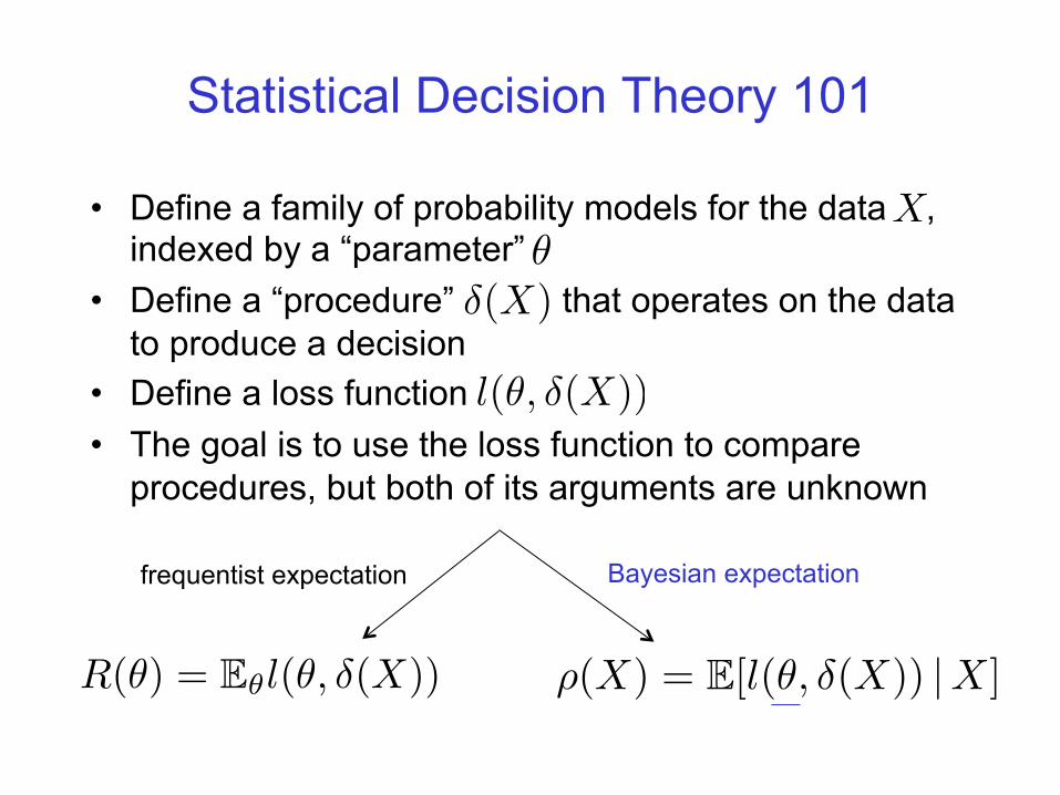
• Define a family of probability models for the data , indexed by a “parameter”
• Define a “procedure” that operates on the data to produce a decision
• Define a loss function • The goal is to use the loss function to compare
procedures, but both of its arguments are unknown
Xθ
δ(X)
l(θ, δ(X))
R(θ) = Eθl(θ, δ(X))
frequentist expectation Bayesian expectation
ρ(X) = E[l(θ, δ(X)) |X]

Statistical Decision Theory 101
• Define a family of probability models for the data , indexed by a “parameter”
• Define a “procedure” that operates on the data to produce a decision
• Define a loss function • The goal is to use the loss function to compare
procedures, but both of its arguments are unknown
Xθ
δ(X)
l(θ, δ(X))
R(θ) = Eθl(θ, δ(X))
frequentist expectation Bayesian expectation
ρ(X) = E[l(θ, δ(X)) |X]

Coherence and Calibration
• Coherence and calibration are two important goals for statistical inference
• Bayesian work has tended to focus on coherence while frequentist work hasn’t been too worried about coherence – the problem with pure coherence is that one can be coherent and
completely wrong
• Frequentist work has tended to focus on calibration while Bayesian work hasn’t been too worried about calibration – the problem with pure calibration is that one can be calibrated and
completely useless
• Many statisticians find that they make use of both the Bayesian perspective and the frequentist perspective, because a blend is often a natural way to achieve both coherence and calibration
The Bayesian World
• The Bayesian world is further subdivided into subjective Bayes and objective Bayes
• Subjective Bayes: work hard with the domain expert to come up with the model, the prior and the loss
• Subjective Bayesian research involves (inter alia) developing new kinds of models, new kinds of computational methods for integration, new kinds of subjective assessment techniques
• Not much focus on analysis, because the spirit is that “Bayes is optimal” (given a good model, a good prior and a good loss)

Subjective Bayes
• A fairly unassailable framework in principle, but there are serious problems in practice – for complex models, there can be many, many unknown
parameters whose distributions must be assessed – independence assumptions often must be imposed to make
it possible for humans to develop assessments – independence assumptions often must be imposed to obtain
a computationally tractable model – it is particularly difficult to assess tail behavior, and tail
behavior can matter (cf. marginal likelihoods and Bayes factors)
• Also, there are lots of reasonable methods out there that don’t look Bayesian; why should we not consider them?
Objective Bayes
• When the subjective Bayesian runs aground in complexity, the objective Bayesian attempts to step in
• The goal is to find principles for setting priors so as to have minimal impact on posterior inference
• E.g., reference priors maximize the divergence between the prior and the posterior
• Objective Bayesians often make use of frequentist ideas in developing principles for choosing priors
• An appealing framework (and a great area to work in), but can be challenging to work with in complex (multivariate, hierarchical) models
Frequentist Perspective
• From the frequentist perspective, procedures can come from anywhere; they don’t have to be derived from a probability model
• This opens the door to some possibly silly methods, so it’s important to develop principles and techniques of analysis that allow one to rule out methods, and to rank the reasonable methods
• Frequentist statistics has tended to focus more on analysis than on methods – but machine learning research, allied with optimization, has
changed that • One general method—the bootstrap
Frequentist Perspective • There is a hierarchy of analytic activities:
– consistency – rates – sampling distributions
• Classical frequentist statistics focused on parametric statistics, then there was a wave of activity in nonparametric testing, and more recently there has been a wave of activity in other kinds of nonparametrics – e.g., function estimation – e.g., small n, large p problems
• One of the most powerful general tools is empirical process theory, where consistency, rates and sampling distributions are obtained uniformly on various general spaces (this is the general field that encompasses much of statistical learning theory)
Outline Part I: Convex relaxations to trade off statistical
efficiency and computational efficiency Part II: Bring algorithmic principles more fully into
contact with statistical inference. The principle in today’s talk: divide-and-conquer
Part I: Computation/Statistics Tradeoffs via Convex
Relaxation
with Venkat Chandrasekaran Caltech

Computation/StatisticsTradeoffs
• More data generally means more computation in our current state of understanding – but statistically more data generally means less risk
(i.e., error) – and statistical inferences are often simplified as the
amount of data grows – somehow these facts should have algorithmic
consequences
Related Work
• Bottou & Bousquet • Shalev-Shwartz, Srebro, et al • Agarwal, et al • Amini & Wainwright • Berthet & Rigollet
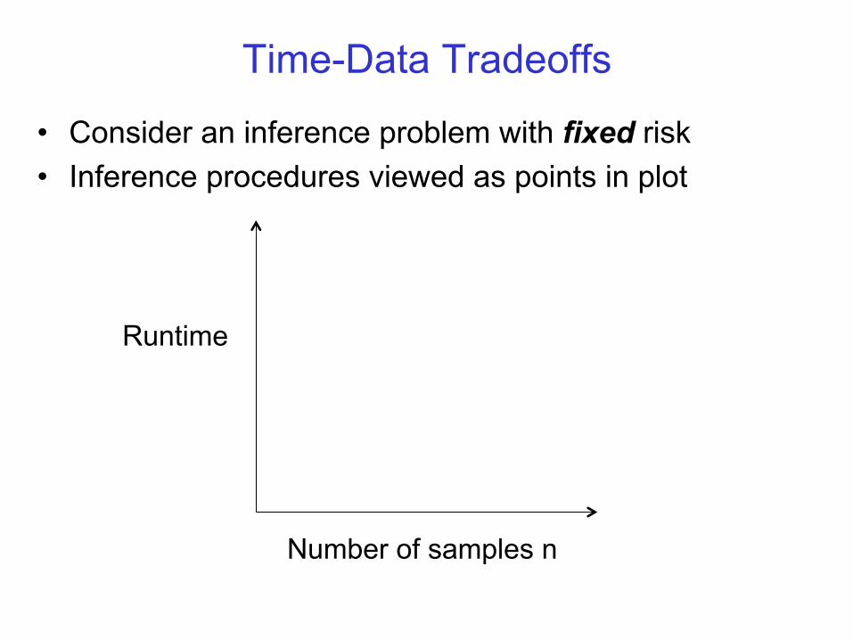
Time-Data Tradeoffs
• Consider an inference problem with fixed risk • Inference procedures viewed as points in plot
Runtime
Number of samples n
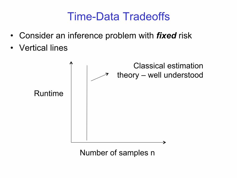
Time-Data Tradeoffs • Consider an inference problem with fixed risk • Vertical lines
Runtime
Number of samples n
Classical estimation theory – well understood
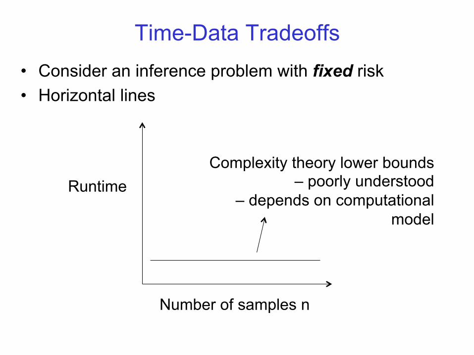
Time-Data Tradeoffs • Consider an inference problem with fixed risk • Horizontal lines
Runtime
Number of samples n
Complexity theory lower bounds – poorly understood
– depends on computational model

Time-Data Tradeoffs • Consider an inference problem with fixed risk
Runtime
Number of samples n
o Trade off upper bounds o More data means smaller
runtime upper bound o Need “weaker”
algorithms for larger datasets
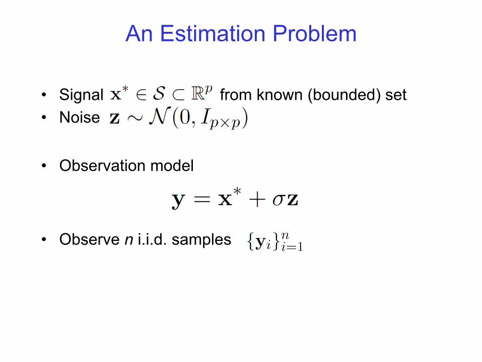
An Estimation Problem
• Signal from known (bounded) set • Noise
• Observation model
• Observe n i.i.d. samples
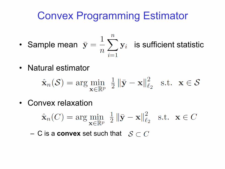
Convex Programming Estimator
• Sample mean is sufficient statistic
• Natural estimator
• Convex relaxation
– C is a convex set such that
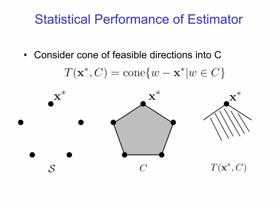
Statistical Performance of Estimator
• Consider cone of feasible directions into C
Statistical Performance of Estimator
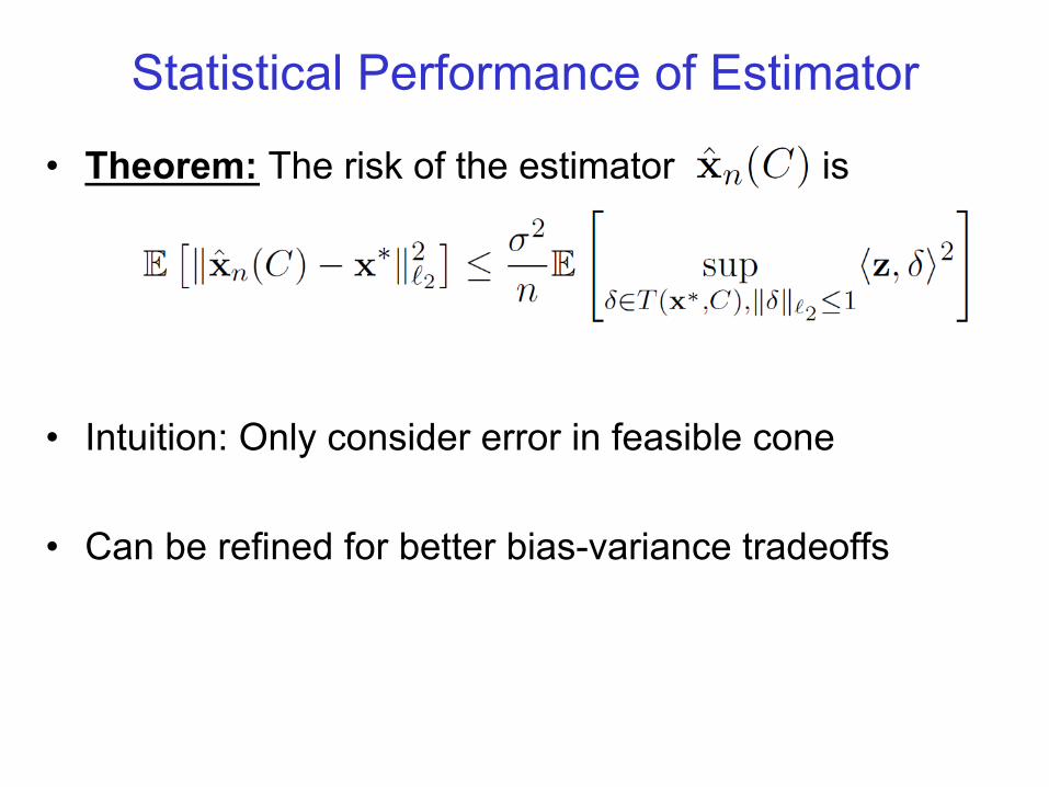
• Theorem: The risk of the estimator is
• Intuition: Only consider error in feasible cone
• Can be refined for better bias-variance tradeoffs
Hierarchy of Convex Relaxations
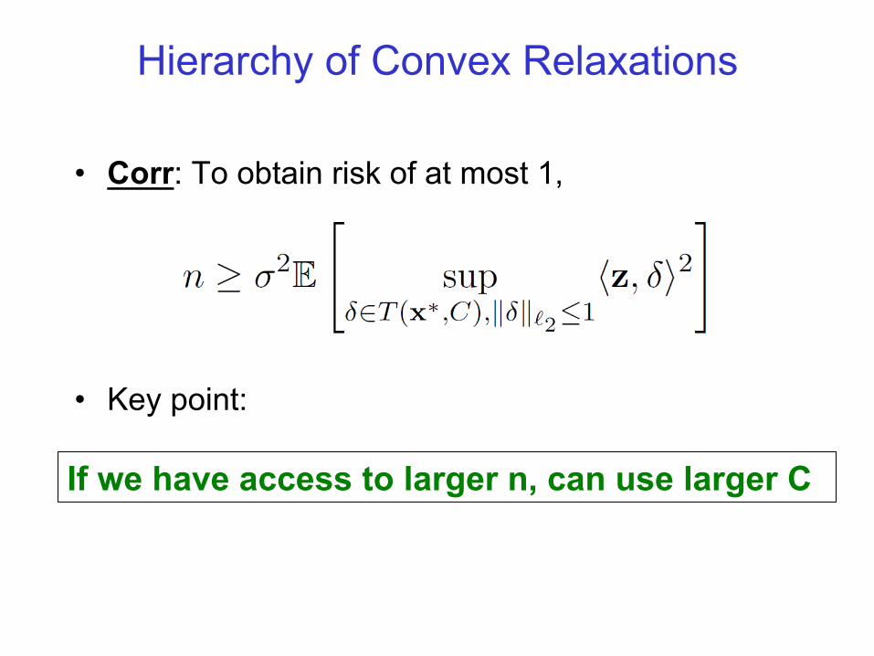
• Corr: To obtain risk of at most 1,
• Key point:
If we have access to larger n, can use larger C
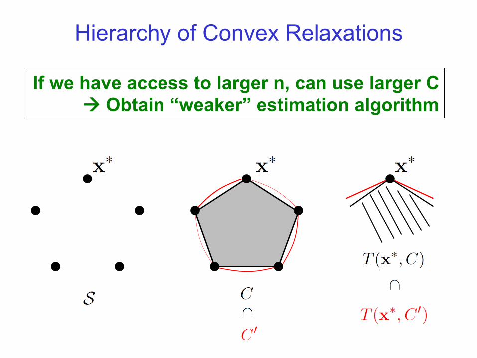
Hierarchy of Convex Relaxations
If we have access to larger n, can use larger C Obtain “weaker” estimation algorithm
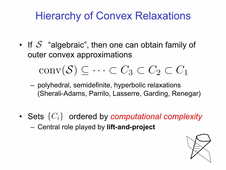
Hierarchy of Convex Relaxations
• If “algebraic”, then one can obtain family of outer convex approximations
– polyhedral, semidefinite, hyperbolic relaxations (Sherali-Adams, Parrilo, Lasserre, Garding, Renegar)
• Sets ordered by computational complexity – Central role played by lift-and-project
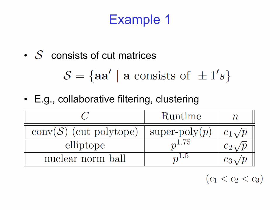
Example 1
• consists of cut matrices
• E.g., collaborative filtering, clustering
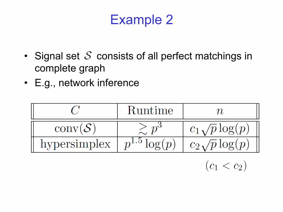
Example 2
• Signal set consists of all perfect matchings in complete graph
• E.g., network inference
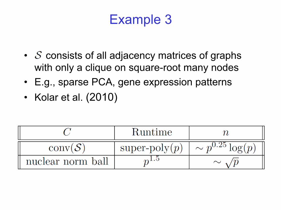
Example 3
• consists of all adjacency matrices of graphs with only a clique on square-root many nodes
• E.g., sparse PCA, gene expression patterns • Kolar et al. (2010)
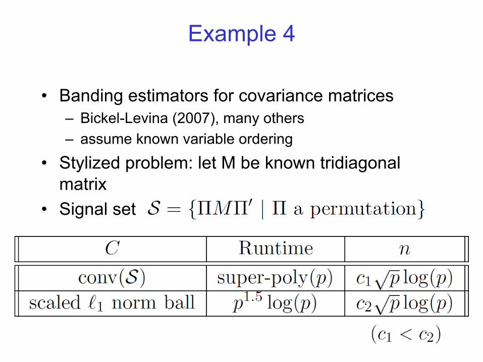
Example 4
• Banding estimators for covariance matrices – Bickel-Levina (2007), many others – assume known variable ordering
• Stylized problem: let M be known tridiagonal matrix
• Signal set
Remarks
• In several examples, not too many extra samples required for really simple algorithms
• Approximation ratios vs Gaussian complexities – approximation ratio might be bad, but doesn’t matter as
much for statistical inference
• Understand Gaussian complexities of LP/SDP hierarchies in contrast to theoretical CS
Part II: The Big Data Bootstrap
with Ariel Kleiner, Purnamrita Sarkar and Ameet Talwalkar
University of California, Berkeley
Assessing the Quality of Inference
• Data mining and machine learning are full of algorithms for clustering, classification, regression, etc – what’s missing: a focus on the uncertainty in the outputs of such
algorithms (“error bars”) • An application that has driven our work: develop a
database that returns answers with error bars to all queries
• The bootstrap is a generic framework for computing error bars (and other assessments of quality)
• Can it be used on large-scale problems?
Assessing the Quality of Inference
Observe data X1, ..., Xn
Assessing the Quality of Inference
Observe data X1, ..., Xn
Form a “parameter” estimate θn = θ(X1, ..., Xn)
Assessing the Quality of Inference
Observe data X1, ..., Xn
Form a “parameter” estimate θn = θ(X1, ..., Xn)
Want to compute an assessment ξ of the quality of
our estimate θn (e.g., a confidence region)
The Unachievable Frequentist Ideal
Ideally, we would ① Observe many independent datasets of size n. ② Compute θn on each. ③ Compute ξ based on these multiple realizations of θn.

The Unachievable Frequentist Ideal
Ideally, we would ① Observe many independent datasets of size n. ② Compute θn on each. ③ Compute ξ based on these multiple realizations of θn.
But, we only observe one dataset of size n.
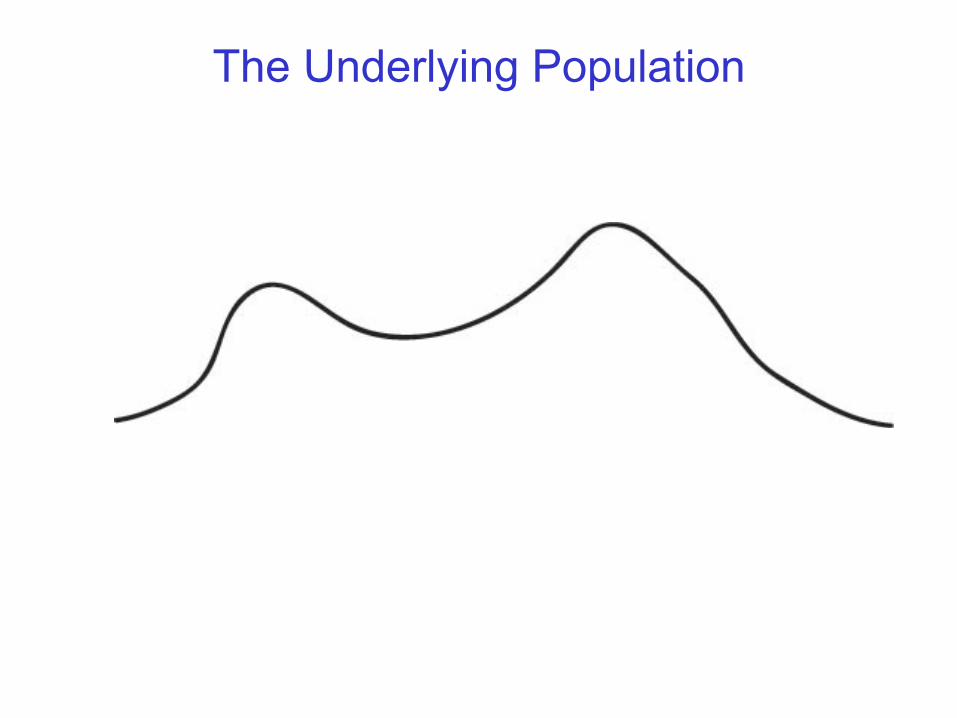
The Underlying Population

The Unachievable Frequentist Ideal
Ideally, we would ① Observe many independent datasets of size n. ② Compute θn on each. ③ Compute ξ based on these multiple realizations of θn.
X(m)1 , . . . , X(m)
n
X(1)1 , . . . , X(1)
n
...
X(2)1 , . . . , X(2)
n
θ(1)n
θ(2)n
θ(m)n
...
ξ(θ(1)n , . . . , θ(m)n )
But, we only observe one dataset of size n.

Sampling

Approximation

Pretend The Sample Is The Population
The Bootstrap
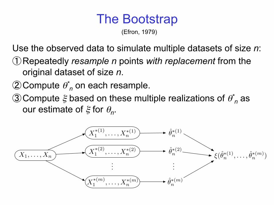
Use the observed data to simulate multiple datasets of size n: ① Repeatedly resample n points with replacement from the
original dataset of size n. ② Compute θ*
n on each resample. ③ Compute ξ based on these multiple realizations of θ*
n as our estimate of ξ for θn.
......
X1, . . . , Xn
X∗(1)1 , . . . , X∗(1)
n
X∗(2)1 , . . . , X∗(2)
n
X∗(m)1 , . . . , X∗(m)
n
θ∗(1)n
θ∗(2)n
θ∗(m)n
ξ(θ∗(1)n , . . . , θ∗(m)n )
(Efron, 1979)

The Bootstrap: Computational Issues
• Seemingly a wonderful match to modern parallel and distributed computing platforms
• But the expected number of distinct points in a bootstrap resample is ~ 0.632n – e.g., if original dataset has size 1 TB, then expect
resample to have size ~ 632 GB • Can’t feasibly send resampled datasets of this
size to distributed servers • Even if one could, can’t compute the estimate
locally on datasets this large
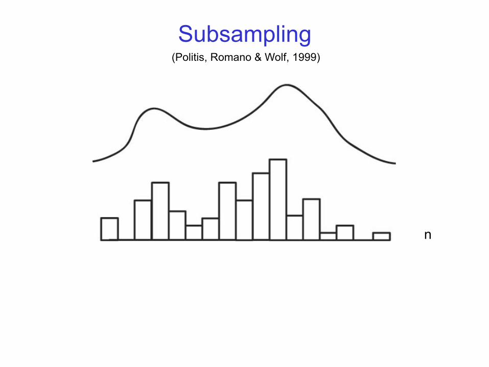
Subsampling
n
(Politis, Romano & Wolf, 1999)

Subsampling
n
b
Subsampling
• There are many subsets of size b < n • Choose some sample of them and apply the estimator to
each • This yields fluctuations of the estimate, and thus error
bars • But a key issue arises: the fact that b < n means that the
error bars will be on the wrong scale (they’ll be too large)
• Need to analytically correct the error bars

Subsampling
Summary of algorithm: ① Repeatedly subsample b < n points without replacement from the
original dataset of size n ② Compute θ*b on each subsample ③ Compute ξ based on these multiple realizations of θ*b ④ Analytically correct to produce final estimate of ξ for θn
The need for analytical correction makes subsampling less automatic than the bootstrap Still, much more favorable computational profile than bootstrap Let’s try it out in practice…
Empirical Results: Bootstrap and Subsampling
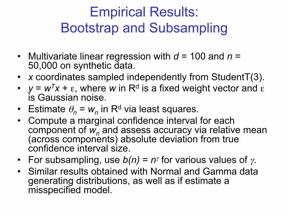
• Multivariate linear regression with d = 100 and n = 50,000 on synthetic data.
• x coordinates sampled independently from StudentT(3). • y = wTx + ε, where w in Rd is a fixed weight vector and ε
is Gaussian noise. • Estimate θn = wn in Rd via least squares. • Compute a marginal confidence interval for each
component of wn and assess accuracy via relative mean (across components) absolute deviation from true confidence interval size.
• For subsampling, use b(n) = nγ for various values of γ. • Similar results obtained with Normal and Gamma data
generating distributions, as well as if estimate a misspecified model.
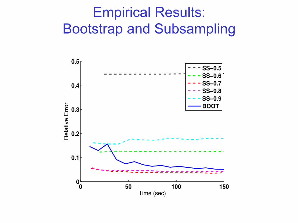
Empirical Results: Bootstrap and Subsampling
0 50 100 1500
0.1
0.2
0.3
0.4
0.5R
ela
tive E
rror
Time (sec)
SS!0.5
SS!0.6
SS!0.7
SS!0.8
SS!0.9
BOOT
Bag of Little Bootstraps
• I’ll now present a new procedure that combines the bootstrap and subsampling, and gets the best of both worlds
Bag of Little Bootstraps
• I’ll now discuss a new procedure that combines the bootstrap and subsampling, and gets the best of both worlds
• It works with small subsets of the data, like subsampling, and thus is appropriate for distributed computing platforms
Bag of Little Bootstraps
• I’ll now present a new procedure that combines the bootstrap and subsampling, and gets the best of both worlds
• It works with small subsets of the data, like subsampling, and thus is appropriate for distributed computing platforms
• But, like the bootstrap, it doesn’t require analytical rescaling
• And it’s successful in practice
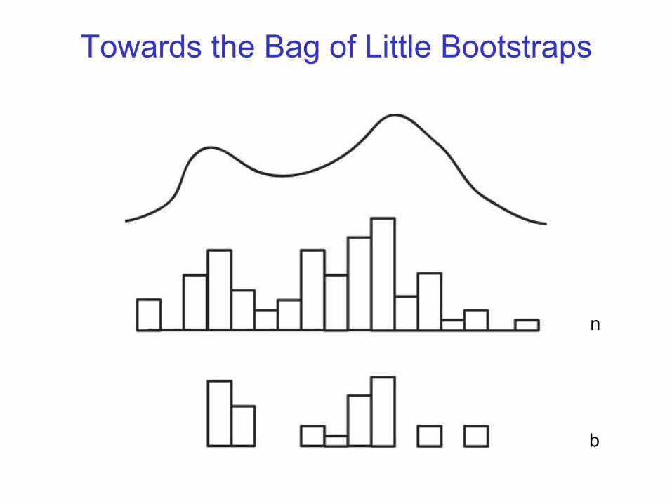
Towards the Bag of Little Bootstraps
n
b

Towards the Bag of Little Bootstraps
b
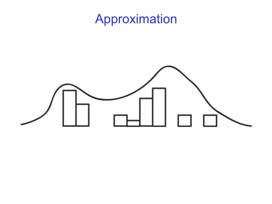
Approximation

Pretend the Subsample is the Population
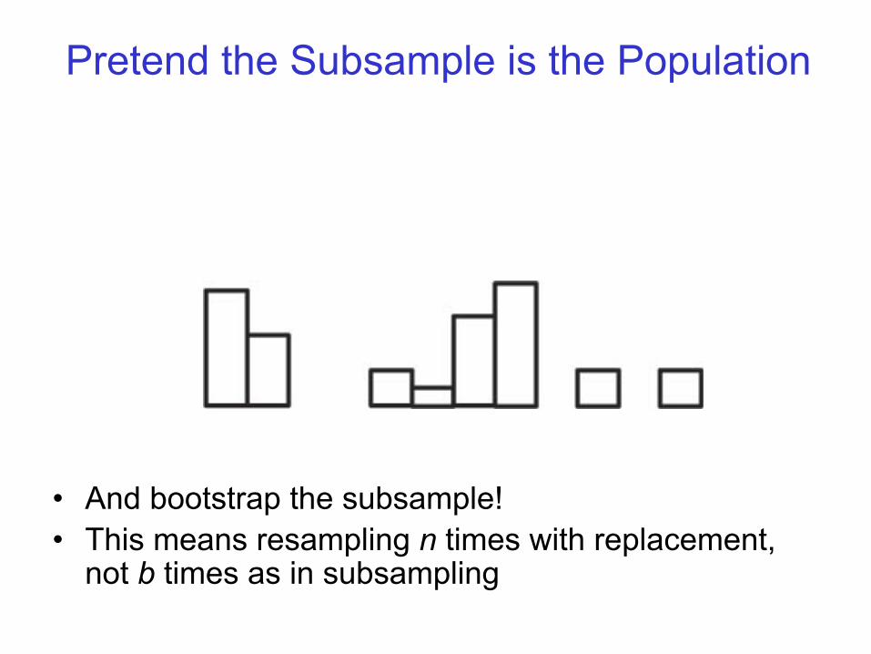
Pretend the Subsample is the Population
• And bootstrap the subsample! • This means resampling n times with replacement,
not b times as in subsampling
The Bag of Little Bootstraps (BLB)
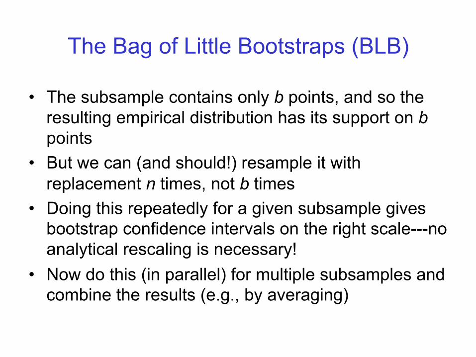
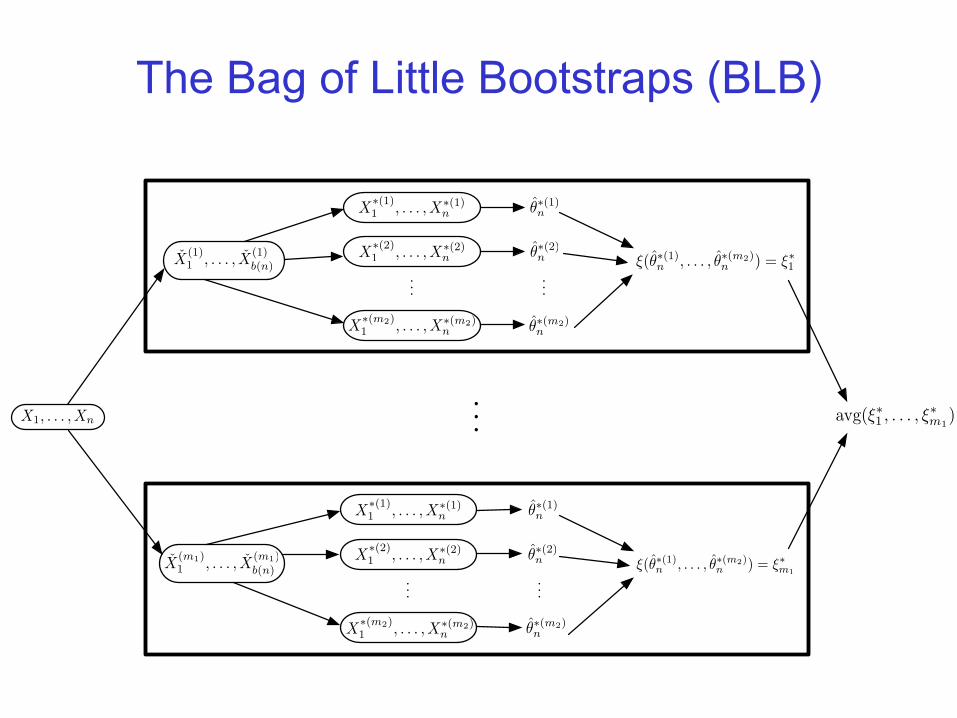
• The subsample contains only b points, and so the resulting empirical distribution has its support on b points
• But we can (and should!) resample it with replacement n times, not b times
• Doing this repeatedly for a given subsample gives bootstrap confidence intervals on the right scale---no analytical rescaling is necessary!
• Now do this (in parallel) for multiple subsamples and combine the results (e.g., by averaging)
The Bag of Little Bootstraps (BLB)
X1, . . . , Xn
......
X∗(1)1 , . . . , X∗(1)
n
X∗(2)1 , . . . , X∗(2)
n
θ∗(1)n
θ∗(2)n
......
X∗(1)1 , . . . , X∗(1)
n
X∗(2)1 , . . . , X∗(2)
n
θ∗(1)n
θ∗(2)n
...
X(1)1 , . . . , X(1)
b(n)
X(m1)1 , . . . , X(m1)
b(n)
X∗(m2)1 , . . . , X∗(m2)
n θ∗(m2)n
X∗(m2)1 , . . . , X∗(m2)
n θ∗(m2)n
ξ(θ∗(1)n , . . . , θ∗(m2)n ) = ξ∗1
ξ(θ∗(1)n , . . . , θ∗(m2)n ) = ξ∗m1
avg(ξ∗1 , . . . , ξ∗m1
)
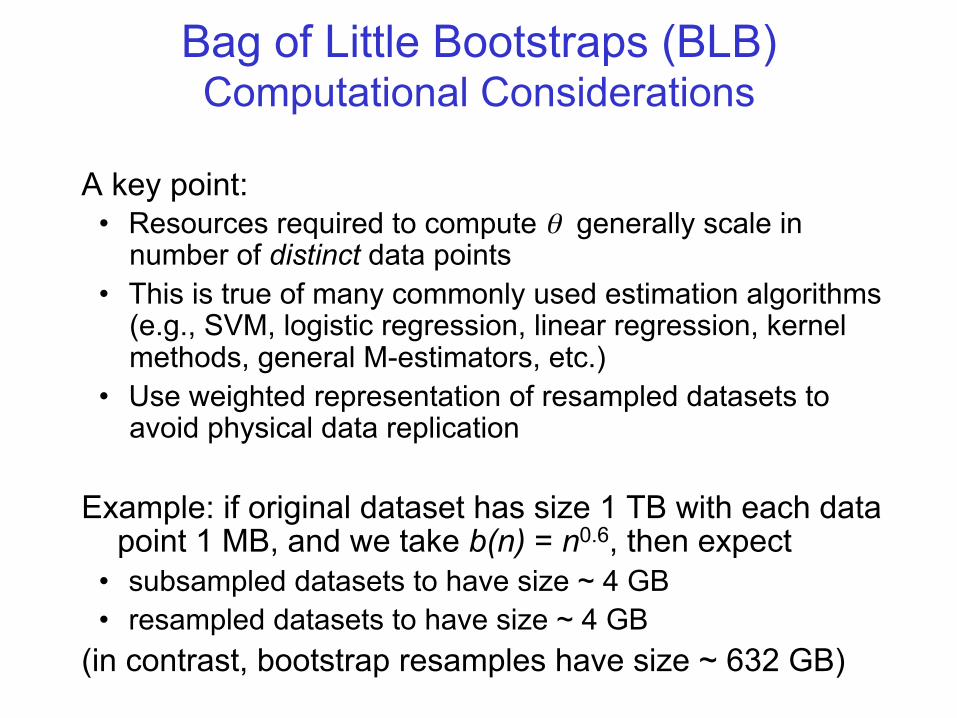
Bag of Little Bootstraps (BLB) Computational Considerations
A key point: • Resources required to compute θ generally scale in
number of distinct data points • This is true of many commonly used estimation algorithms
(e.g., SVM, logistic regression, linear regression, kernel methods, general M-estimators, etc.)
• Use weighted representation of resampled datasets to avoid physical data replication
Example: if original dataset has size 1 TB with each data
point 1 MB, and we take b(n) = n0.6, then expect • subsampled datasets to have size ~ 4 GB • resampled datasets to have size ~ 4 GB
(in contrast, bootstrap resamples have size ~ 632 GB)
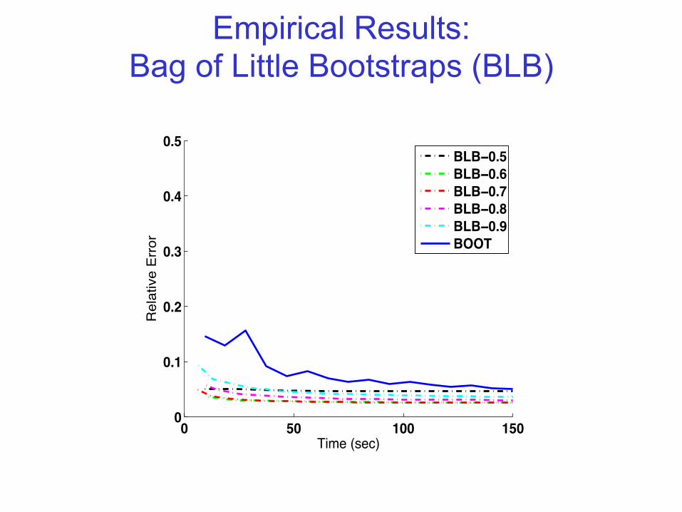
Empirical Results: Bag of Little Bootstraps (BLB)
0 50 100 1500
0.1
0.2
0.3
0.4
0.5R
ela
tive E
rror
Time (sec)
BLB!0.5
BLB!0.6
BLB!0.7
BLB!0.8
BLB!0.9
BOOT
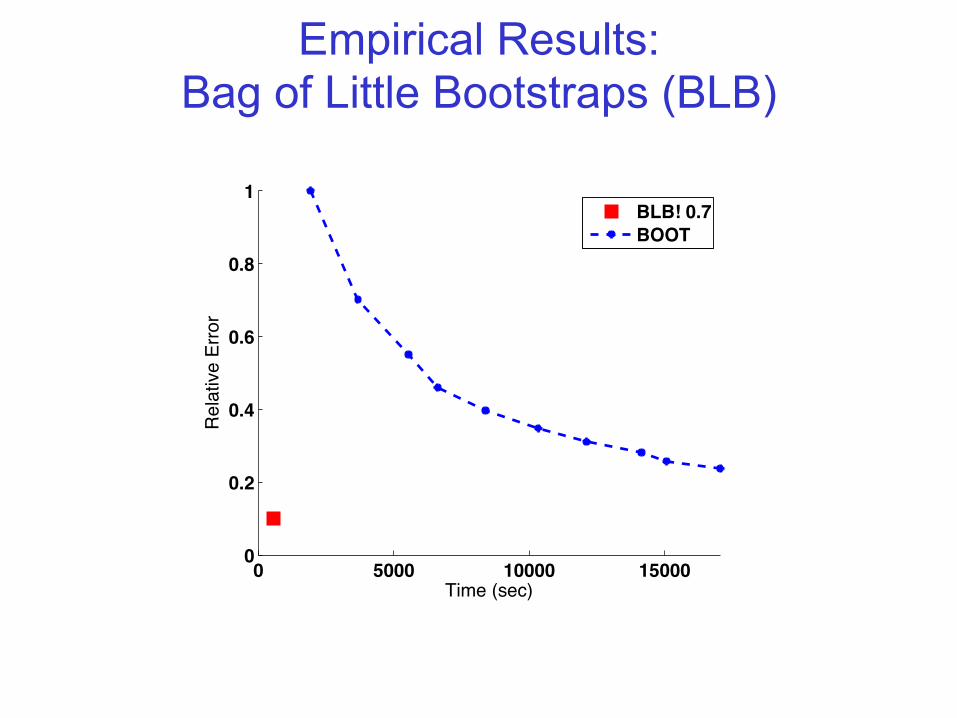
Empirical Results: Bag of Little Bootstraps (BLB)
0 5000 10000 150000
0.2
0.4
0.6
0.8
1
Rela
tive E
rror
Time (sec)
BLB! 0.7
BOOT
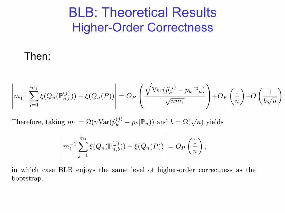
BLB: Theoretical Results Higher-Order Correctness
Then:
m
−11
m1
j=1
ξ(Qn(P(j)n,b))− ξ(Qn(P ))
= OP
Var(p(j)k − pk|Pn)
√nm1
+OP
1
n
+O
1
b√n
Therefore, taking m1 = Ω(nVar(p(j)k − pk|Pn)) and b = Ω(√n) yields
m
−11
m1
j=1
ξ(Qn(P(j)n,b))− ξ(Qn(P ))
= OP
1
n
,
in which case BLB enjoys the same level of higher-order correctness as thebootstrap.
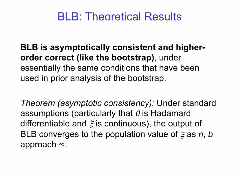
BLB: Theoretical Results
BLB is asymptotically consistent and higher-order correct (like the bootstrap), under essentially the same conditions that have been used in prior analysis of the bootstrap. Theorem (asymptotic consistency): Under standard assumptions (particularly that θ is Hadamard differentiable and ξ is continuous), the output of BLB converges to the population value of ξ as n, b approach ∞.
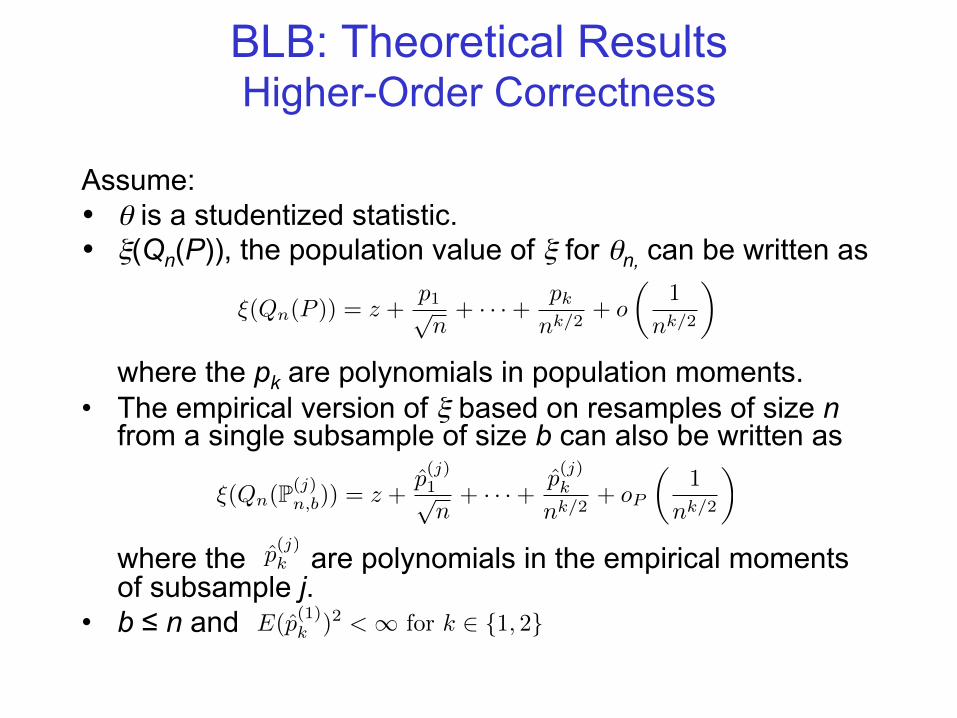
BLB: Theoretical Results Higher-Order Correctness
Assume: • θ is a studentized statistic. • ξ(Qn(P)), the population value of ξ for θn, can be written as
where the pk are polynomials in population moments.
• The empirical version of ξ based on resamples of size n from a single subsample of size b can also be written as
where the are polynomials in the empirical moments of subsample j.
• b ≤ n and
ξ(Qn(P )) = z +p1√n+ · · ·+ pk
nk/2+ o
1
nk/2
ξ(Qn(P(j)n,b)) = z +
p(j)1√n
+ · · ·+p(j)k
nk/2+ oP
1
nk/2
p(j)k
E(p(1)k )2 < ∞ for k ∈ 1, 2
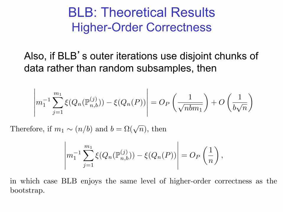
BLB: Theoretical Results Higher-Order Correctness
Also, if BLB’s outer iterations use disjoint chunks of data rather than random subsamples, then
m
−11
m1
j=1
ξ(Qn(P(j)n,b))− ξ(Qn(P ))
= OP
1√
nbm1
+O
1
b√n
Therefore, if m1 ∼ (n/b) and b = Ω(√n), then
m
−11
m1
j=1
ξ(Qn(P(j)n,b))− ξ(Qn(P ))
= OP
1
n
,
in which case BLB enjoys the same level of higher-order correctness as thebootstrap.
Conclusions
• Many conceptual challenges in Big Data analysis • Distributed platforms and parallel algorithms
– critical issue of how to retain statistical correctness – see also our work on divide-and-conquer algorithms for
matrix completion (Mackey, Talwalkar & Jordan, 2012) • Algorithmic weakening for statistical inference
– a new area in theoretical computer science? – a new area in statistics?
• For papers, see www.cs.berkeley.edu/~jordan