bikeability in basel · a.1 case study basel ..... 77 a.2 using the dependency between cyclists’...
TRANSCRIPT

Bikeability in Basel
Elena Grigore
Master Thesis
Spatial Development and Infrastructure Systems
July 2018

Bikeability in Basel July 2018
2
Preface
There is growing interest in transport communities to promote sustainable transport modes,
such as walking and cycling. Due to their space- and resource efficiency, they have the
potential to reduce congestion in inner cities. While the concept of walkability has been a
popular research topic for many years, bikeability has been given less attention. The objective
of this thesis is to develop a method to model “bikeability” within the Swiss context. The
method will enable the identification of locations where improvements are necessary, as well
the quantification of different planning measures. A case study area within the city of Basel
has been selected for assessment.
In order to develop the tool, the workflow has been structured according to the following
steps:
Relevant literature and data sources are reviewed and described. This concerns
existing methods to assess bikeability and walkability, as well as literature regarding
the attributes of streets and intersections that are important for cyclists.
A relevant case study area is chosen within the city of Basel.
A method to model bikeability of the area is developed based on the findings from the
literature review.
The assessment is carried out with the software QGIS for the case study area.
Afterwards, important findings and recommendations are discussed. A sensitivity
analysis is carried out to see how bikeability is affected by changes in the quality of
the network. Possible applications are discussed.
As a final step, the method is evaluated according to its strengths and limitations, and
possibilities for expansion are discussed. Interesting topics for further research are
identified and discussed.
This research has been done at the Chair for Transport Planning, under the leading of Prof.
Dr. K. W. Axhausen, supervised by Prof. Dr. N. W. Garrick and Raphael Fuhrer, in
collaboration with the Office of Mobility of Canton Basel-Stadt.

Bikeability in Basel July 2018
3
Acknowledgements
Hereby, I would like to thank Prof. Dr. K.W. Axhausen for making this project possible. A
special thanks to my supervisors Prof. Dr. N. W. Garrick and Raphael Fuhrer for their
supervision of the project. Due to their useful insights and their openness for discussion, they
helped bringing the project forward.
I would also like to thank my supervisors and colleagues from the Office of Mobility Basel-
Stadt for their collaboration, interesting ideas and for providing the necessary data. My thanks
go to Barbara Auer, Simon Kettner, Alain Groff, Thomas Graff, Michael Redle and Andrea
Dürrenberger.
Finally, I would like to thank my family, partner and friends for their support during this project,
as well as during my whole study period.

Bikeability in Basel July 2018
4
Master Thesis
Bikeability in Basel
Elena Grigore
IVT ETH Zurich
Seestrasse 266, 8038 Zurich, Switzerland
Phone: +41- 767278162
E-Mail: [email protected]
July 2018
Abstract
“Bikeability” is becoming increasingly relevant in the fields or transport- and spatial planning.
However, it is not always clear how bikeability is defined, let alone how it can be modeled. The
goal of this project is to develop a method to model bikeability within the Swiss context. A case
study area in the city of Basel has been selected for analysis. In this thesis, “bikeability” is
understood as a measure of the ability and convenience to reach important destinations by bike,
based on the quality of the routes and the travel distances. Results show that the method
developed enables the identification of locations where improvements in the cycling network
are necessary. Moreover, it allows the quantification of various planning measures, by assessing
their effect on bikeability. The current analysis is intended for conventional bikes and is focused
on the needs of commuting cyclists. However, the method can be expanded to consider E-bikes
and non-commuting cyclists.
Keywords
Bikeability; Perceived distance; Cycling quality; Accessibility; Cyclist; Route choice;
Transport planning; Spatial Planning; Urban design; Sustainable transport
Preferred citation style
Grigore, E. (2018) Bikeability in Basel, Master Thesis, Institute for Transport Planning
and Systems, ETH Zurich, Zurich.

Bikeability in Basel July 2018
5
Table of contents
1 Introduction ....................................................................................................................... 12
2 Literature review ............................................................................................................... 13
2.1 Measuring bikeability and walkability ...................................................................... 13
3 Methodology ..................................................................................................................... 19
3.1 Case Study Basel ....................................................................................................... 19
3.2 Overview and scope of the project ............................................................................ 20
3.3 Cycling quality for streets.......................................................................................... 21
3.4 Cycling quality of intersections ................................................................................. 33
3.5 Perceived distance along a route ............................................................................... 37
3.6 Bikeability and accessibility by bike ......................................................................... 37
3.7 Spatial data ................................................................................................................ 39
3.8 Assumptions and simplifications ............................................................................... 40
3.9 Correlations ............................................................................................................... 43
4 Results ............................................................................................................................... 44
4.1 Cycling quality of street segments ............................................................................. 44
4.2 Cycling quality of intersections ................................................................................. 50
4.3 Bikeability and accessibility by bike ......................................................................... 53
5 Findings and recommendations ........................................................................................ 56
5.1 Overview ................................................................................................................... 56
5.2 Identifying locations where network improvements are necessary ........................... 56
5.3 Sensitivity analysis .................................................................................................... 59
5.4 Computing bikeability and accessibility for only one destination ............................ 63
5.5 The influence of segment attributes on sensitivity .................................................... 65
5.6 Application in urban planning ................................................................................... 66
6 Conclusion ........................................................................................................................ 68
6.1 Evaluation of the research method ............................................................................ 68
6.2 Further research ......................................................................................................... 70
7 References ......................................................................................................................... 71

Bikeability in Basel July 2018
6
A Additional information regarding methodology ............................................................... 77
A.1 Case study Basel ........................................................................................................ 77
A.2 Using the dependency between cyclists’ speed and gradient to determine the gradient
cost function ......................................................................................................................... 79
A.3 Comparison between Swiss, Dutch, and Danish guidelines regarding the types of
cycling infrastructure ............................................................................................................ 80
A.4 Comparison between the chosen gradient cost function, and the cost function found
by Broach et al. (2012) ......................................................................................................... 82
A.5 Comparison between the chosen cycling infrastructure cost functions, and the cost
function found by Broach et al. (2012) ................................................................................ 83
A.6 Example of a roundabout cost calculation ................................................................. 84
B Additional information regarding spatial data .................................................................. 85
B.1 The street network ..................................................................................................... 85
B.2 Workspaces ................................................................................................................ 87
C Additional information regarding calculations ................................................................. 87
C.1 Computing the gradient ............................................................................................. 87
C.2 Computing the coverage of green and water ............................................................. 87
C.3 Generating intersections and annotating segments with intersection IDs ................. 88
C.4 Cost calculation for segments and intersections ........................................................ 88
C.5 Computing the shortest perceived path with the Dijkstra algorithm ....................... 100
C.6 Declaration of originality ......................................................................................... 103

Bikeability in Basel July 2018
7
List of tables
Table 1: Types of cycling infrastructure recommended for different motorized traffic volumes
and speed limits in Basel, according to the Swiss and cantonal guidelines ............................. 25
Table 2: Cost functions and constant costs for different types of cycling infrastructure for
different widths ........................................................................................................................ 29
Table 3: Chosen hazards and their costs .................................................................................. 31
Table 4: Turn costs for different types of turns, as identified by Broach et al. (2012) ............ 33
Table 5: Chosen turn cost components and values as a distance measure (m), based on the
findings of Broach et al. (2012) ............................................................................................... 35
Table 6: Additional expansion / reduction of turn cost to account for the intersection layout 36
Table 7: Case studies for the calculation of the cost multiplier ............................................... 49
Table 8: Case studies for turn costs values .............................................................................. 52
Table 9: Synthesis results of Bikeability and accessibility by bike ......................................... 55
Table 10: Average bikeability- and accessibility to workplaces by bike for the Base Scenario,
Scenario Optimization and Scenario Deterioration .................................................................. 61
Table 11: Average values for bikeability and accessibility for the computation with
workplaces as destinations and for the one with Basel SBB as destination ............................. 64
Table 12: Comparison between Swiss, Dutch and Danish guidelines and recommendations . 81
Table 13: Description of the important fields in the segment layer (including intersections) . 86

Bikeability in Basel July 2018
8
List of figures
Figure 1: Selected case study area to be assessed in Basel (shown in red) .............................. 20
Figure 2: Chosen gradient cost function .................................................................................. 23
Figure 3: Chosen cycling infrastructure cost functions for the cases “Bikes + motorized” and
bike lanes (for widths between 1.5 m – 1.8 m), for speed limits of 30 and 50 Km/h .............. 27
Figure 4: Benefit function of the riding environment based on the coverage of green and water
within a 20 m buffer along the street ........................................................................................ 32
Figure 5: Cycling quality for segments in the case study area for both directions of travel .... 44
Figure 6: Gradient costs for both directions of travel .............................................................. 45
Figure 7: Cycling infrastructure costs for both directions of travel ......................................... 46
Figure 8: Hazard costs for both directions of travel ................................................................. 47
Figure 9: Riding environment benefit, based on the percentage of green- and water coverage
.................................................................................................................................................. 48
Figure 10: Number of traffic streets without cycling infrastructure for direct left turns, for
each intersection in the case study area .................................................................................... 50
Figure 11: Bikeability to workplaces (left) and accessibility to workplaces by bike (right) ... 53
Figure 12: Accessibility to workplaces by bike against bikeability to workplaces ................. 54
Figure 13: The cumulative cost for a cycling trip based on actual distance compared to the
cumulative cost for a cycling trip based on perceived distance ............................................... 57
Figure 14: Difference between the average perceived distances to workplaces and the average
scaled real distances for the case study area. Orange spots represent poorly connected areas,
while green spots indicate good connectivity .......................................................................... 58
Figure 15: Scenario Optimization (left) and Scenario Deterioration (right) ............................ 59
Figure 16: Bikeability to workplaces for Scenario Optimization (left) and Scenario
Deterioration (right) as absolute values (top) and as differences from the Base Scenario
(bottom) .................................................................................................................................... 60
Figure 17: Chosen source cell from the case study area (left) and its distribution of perceived
distances for the Base Scenario and Scenario Optimization (right) ......................................... 62
Figure 18: Bikeability and accessibility by bike to Basel SBB for the case study area ........... 63
Figure 19: Distribution of costs among the segments for the total cost (top left), gradient cost
(top right), cycling infrastructure costs (bottom left) and hazard costs (bottom right) ............ 65

Bikeability in Basel July 2018
9
Figure 20: Network map of the Cycling Directive Plan of Canton Basel-Stadt. Commuting
routes are shown in blue, basic routes are shown in red. Source: The Office of Mobility Basel-
Stadt (2014) .............................................................................................................................. 77
Figure 21: Traffic oriented streets in Basel-Stadt, classified into motorways (yellow), main
connection roads (red) and main collection streets (green) ...................................................... 78
Figure 22: Map of the streets and intersections mentioned in sections 4.1 and 4.2.
Intersections are marked with the sign “-“ between the names of the streets .......................... 79
Figure 23: Design speed (y-axis) vs. longitudinal gradient (x-axis). Speed 0 represents the
speed of cyclist on a flat surface. ............................................................................................. 80
Figure 24: Comparison between the chosen gradient cost function, and the gradient cost
determined in the route choice model by Broach et al. (2012) ................................................ 82
Figure 25: Comparison between the chosen cycling infrastructure cost functions, and the cost
function determined in the route choice model by Broach et al. (2012) for cycling together
with motorized transportation .................................................................................................. 83
Figure 26: Example of cycling trajectory through a roundabout ............................................. 84
Figure 27: Weighting factor for the cycling infrastructure costs against bike lane widths
between 1.2 m and 1.5 m .......................................................................................................... 89
Figure 28: Assigning virtual starting- and ending nodes at each intersection, with virtual
segments of lengths 0 m ........................................................................................................... 90
Figure 29: Declaration of originality ...................................................................................... 103

Bikeability in Basel July 2018
10
List of abbreviations
AADT: Annual Average Daily Traffic
ASTRA: Swiss Federal Roads Office
ARE: Swiss Federal Office for Spatial Development
BLOS: bicycle level of service
BVB: Basler Verkrhs Betriebe (Board of city tranport in Basel-Stadt)
BVD: Department of Construction and Transport Basel-Stadt
CROW: Dutch Bicycle Design Manual
DWV: Annual Average Daily Traffic for weekdays
DTV: Annual Average Daily Traffic (in German)
HCM: Highway Capacity Manual
TBA: Department of Civil Engineering Base-Stadt
TRB: Transport Research Board
UVEK: Swiss Federal Department for the Environment, Transport, Energy and
Communications
veh.: vehicle
VSS: Swiss Association of Road and Traffic Professionals
List of symbols
𝑎𝑖: accessibility of destination i (based on Hansen’s model)
𝐵𝐸𝑛𝑣: riding environment benefit
𝑏𝑖: bikeability of source i
𝛽: parameter that determines how strongly distance impedes travel
𝐶𝑏𝑙: cycling infrastructure cost for bike lanes
𝐶 𝑏𝑚: cycling infrastructure cost for the case bike + motorized (bikes riding together with cars)
𝐶𝐺𝑟: gradient cost

Bikeability in Basel July 2018
11
𝐶𝑖𝑗: travel cost from souce i to destination j
𝐶𝐼𝑛𝑓: cycling infrastructure cost
𝐶𝐻𝑧: hazard cost
𝐶𝑡: turn cost
𝐷: subset of destination (hectare centers)
de: end point of a segment in the direction DR
DR: predefined direction of travel for each segment
ds: starting point of a segment in the direction DR
𝐸𝑗 : intensity of activity at destination j (e.g number of workplaces)
f, g, h: parameters of an exponential function
ge: end point of a segment in the direction GDR
GDR: direction of travel opposite to the predefined direction for each segment
gs: starting point of a segment in the direction GDR
𝑔𝑟: gradient of a street segment, measured in percentage
𝑔𝑤 𝑝𝑒𝑟: percentage of green and water coverage
𝐼𝑖𝑗: subset of intersections along the route from source i to destination j
𝐿𝑠: length of segment s in m
𝑀 𝑠: cost multiplier for one street segment
𝑝𝑖𝑗: perceived distance along the route from source i to destination j
𝑅𝑖𝑗: subset of segments along the route from source i to destination j
𝑠: segment
𝑡: turn
𝑊𝑓: weighting factor (used to compute the cycling infrastructure cost for bike lanes with widths
between 1.2 m and 1.5 m)
𝑊𝑖𝑏𝑙: bike lane width
𝑤𝑗: number of workplaces at destination j

Bikeability in Basel July 2018
12
1 Introduction
Cycling as a sustainable transport mode has become increasingly relevant in transport- and
spatial planning, because it has the potential to replace motorized transportation for short
distances. Cycling is space-efficient, does not cause pollution, and is financially attractive.
Moreover, it can be perceived as a form of leisure and has many health benefits. Therefore,
many cities are aiming at increasing their modal share of cycling by improving the
attractiveness of their cycling network. However, it is not always clear how to quantify the
influence of various cycling measures, nor for which locations in the network improvements
are relevant.
Therefore, the goal of this project is to develop a method to model bikeability within the
Swiss context, using Basel as a case study. In this thesis, bikeability is understood as a
measure of the ability and convenience to reach important destinations by bike, based on the
quality of the routes and the travel distances. However, it is important to note that there is no
consensus in literature about the definition of the term. In many research papers, “bikeability”
refers only to the quality of streets for cycling.
The assessment consists of three main components: first, the quality of streets and
intersections is evaluated according to a number of attributes selected and quantified
according to literature. As a second component, a measure of perceived distance for cycling
routes is defined based on the quality of streets and intersections along a route. Afterwards,
the perceived distances to the destinations of interest will be used to compute bikeability for
each cell in the case study area. The analysis will be carried out using the software QGIS.
For simplicity, the analysis will focus only on conventional bikes and commuter cyclists.
Therefore, the method will not be directly applicable to assess bikeability for E-Bikes and
non-commuter cyclists. Moreover, the assessment will be carried out for a case study area in
Basel and will only consider workplaces and the train station SBB as destinations.
Nevertheless, various expansions of the method are possible and will be discussed.

Bikeability in Basel July 2018
13
2 Literature review
2.1 Measuring bikeability and walkability
2.1.1 Defining “bikeability”
The term “bikeability” is used differently in literature. In some studies, the term is used to assess
the quality of streets in an urban area, according to their level of comfort and safety for cyclists
(e.g. Krenn et al. (2015)). However, assessing the quality of streets is not sufficient to locate
where improvements in the network are necessary, because some streets might be located along
more important routes than others. In this respect, a more comprehensive approach is observed
in the work of Lowry et al. (2012). Their assessment of bikeability incorporates both the quality
of streets and intersections, as well as the accessibility to the destinations of interest by bike.
The current thesis adopts a similar approach, whereby bikeability is defined as an assessment
of the ability and convenience to reach important destinations by bike, based on the routes’
cycling quality and the travel distances. The cycling quality will be defined in terms of
perceived comfort, safety and attractiveness of streets and intersections composing the cycling
routes. This concept is also referred to as “bicycle suitability” in literature (Lowry et al, 2012).
2.1.2 Methods to evaluate the cycling quality
There are many existing methods to evaluate the cycling quality. In most cases, various
attributes of the street are assessed and they receive a number of points, which are combined
into a total score. However, the choice of attributes, and the score calculation are different for
each method (Lowry et al., 2012).
One of the most frequently used methods is the bicycle level of service (BLOS), which enables
the evaluation of both streets and intersections. The method is described in the Highway
Capacity Manual (HCM) of the Transportation Research Board (TRB, 2000). The attributes
used to assess the cycling quality of streets are vehicle volumes (including heavy traffic),
vehicle speeds and bicyclists’ operating space (width of the outside lane, of the shoulder, or of
the bike lane). For the intersection, BLOS is primarily a function of the width of the street being
crossed, the bicyclists’ operating space, as well as of traffic volumes (Huff & Ligett, 2014).
However, BLOS has a few shortcomings: first of all, it does not consider attributes that are not
related to infrastructure, such as topography and landscape quality. According to Broach et al.
(2012), avoiding steep uphill slopes is the main reason for cyclists to detour from the shortest
route. Second of all, BLOS is not sensitive to bicycle specific intersection treatments, such as

Bikeability in Basel July 2018
14
bike boxes, and does not consider the presence of cycle tracks (Huff & Ligett, 2014). Third of
all, BLOS has been developed for US, and further research is needed to determine whether it is
directly applicable in a European context. Therefore, BLOS will not be used to measure cycling
quality for the current project.
Instead of using an existing method to evaluate the cycling quality, one can develop a cycling
index that can be applied specifically for the area to be evaluated. Its components can be
identified and quantified by comparing cyclists’ GPS traces with the shortest possible cycling
routes. If a cyclist chooses to travel longer than the shortest distance, a reasonable explanation
is that the longer route provides better comfort or safety. Winters et al. (2013) and Krenn et al.
(2015) conducted such analyses in Vancouver and in Graz respectively and each of them have
developed a cycling index (referred to as bikeability index in their work). The indices consist
of five components that are additively combined to produce a total score. Their calculations and
mapping of the cycling quality has been conducted in GIS.
Broach et al. (2012) used a comparison of GPS traces with the shortest routes in Portland, to
develop a route choice model for cyclists. The importance of each relevant street and
intersection attribute is quantified based on how long cyclists are willing to detour from their
shortest route, in order to avoid, or to encounter a certain attribute along their way. Their
findings suggest that the average detour from the shortest path amounts to 11-12%. Similar
studies find longer average detours, such as 40% (Sener et.al., 2009) and 67% (Krizek et al.,
2007).
However, an analysis based on GPS data goes beyond the scope of this project. The selection
and quantification of the cycling quality attributes will be based on existing literature, as well
as norms, guidelines and recommendations (see sections 3.3 and 3.4).
2.1.3 Attributes of streets and intersections regarding cycling quality
The decision to cycle depends on many factors, such as travel distance to destinations, trip
purpose and the individual characteristics of cyclists (ASTRA, 2017). Numerous studies show
that the characteristics of streets and intersections are crucial in determining the cyclists’
perceived safety and comfort, and hence their decision to cycle (Caviedes et al., 2016; Broach
et al., 2012; Menghini et al., 2009). In this section, the attributes of streets and intersections
important for cyclists are identified from literature and explained.
An important factor regarding cyclists’ comfort is the inclination of streets, known as “gradient”
(ASTRA, 2017). Both Winters et al. (2013) and Krenn et al. (2015) identify the gradient as one
of the five components of their cycling indices. Broach et al. (2012) find that commuter cyclists

Bikeability in Basel July 2018
15
will detour longer than three times the shortest distance in order to avoid slopes higher than 6%,
while Menghini et al. (2009) also find that gradients of 5.6% are avoided. Uphill slopes require
a higher physical effort for cyclists to maintain the same speed on a flat surface and therefore
they reduce the directness of a route, according to the Swiss Guideline for the Planning of
Cycling Routes (ASTRA et al., 2008). Additionally, it is harder for cyclists to keep balance on
an uphill slope, as it is pointed out by Baker & Schmidt (2017) in Basel’s Cantonal Design
Guideline for Cycling and Pedestrian Traffic. At the same time, cycling downhill can be
dangerous due to high cycling speeds, especially near parked cars, according to the Technical
Report of Basel’s Cycling Directive Plan (Pestalozzi & Stäheli, 2012).
Furthermore, the speed limits and the motorized traffic volumes can impact the cyclists’
comfort and safety. The car speed affects both the collision risk between a car and a bike and
the severity of the accident (Schüller, 2017). Broach et al. (2012) find that streets with high
motorized traffic volumes are avoided by cyclists, when there is no cycling infrastructure
available. According to the Swiss, Dutch and Danish cycling guidelines, bikes should not ride
together with cars for speed limits higher than 30 - 40 Km/h and for motorized traffic volumes
higher than 3000 veh./day (ASTRA et al., 2008; CROW, 2007; Celis Consult, 2014). The
percentage of heavy traffic should not exceed 8% along cycling routes (ASTRA et al., 2008).
Of course, different types of cycling infrastructure are evaluated differently by cyclists.
Generally, separated tracks are perceived as safer than bike lanes, although more accidents
occur at intersections with cycle tracks than with bike lanes (Agerholm et al., 2006; Jensen,
2006). Cyclists prefer not to share the same path with pedestrians, due to the risk of collision
with pedestrians (Walter, 2017a). Moreover, they prefer homogenous routes, where the type of
cycling infrastructure remains constant over longer distances (ASTRA et al., 2008). Different
widths are recommended for different types of cycling infrastructure, in order to provide the
desired level of comfort (Baker & Schmidt, 2017). The presence of car parking and tram tracks
can lead to dangerous situations for cyclists and can be perceived as hazards. These are
problematic especially in combination with insufficient space or downhill slopes (Pestalozzi &
Stäheli, 2012). Certain street layouts can lead to dangerous overtaking situations in mixed
traffic, when the motorized traffic volumes are too high for the given street width (ASTRA et
al., 2008) (see section 3.3).
Krenn et al. (2015) identify the presence of green and aquatic areas as one of the five
components of their cycling index. Green and water positively contribute to the attractiveness
of bike routes due to their aesthetics, but also because they provide shade and cooling in the
summer. ASTRA et al. (2008) recommend the presence of green and water along cycling routes.

Bikeability in Basel July 2018
16
Other attributes of streets that are positively perceived by cyclists are smooth surfaces, presence
of lightning, proper signalization, and lack of interruptions (ASTRA et al., 2008; Hausigke,
2018). ). However, these factors are found less frequently in literature than the others, and have
not been identified by the route choice models reviewed. Therefore, they will not be included
in the analysis.
Most of existing bikeability assessments consider only the quality of streets, without
incorporating intersection design. However, intersections are a source of conflict and delay
for cyclists. According to Dill et al. (2011), 68% of bicycle crashes occur at intersections. The
bicycle accident map in Basel also shows that many accidents involving bicycles occur near
intersections (Swisstopo, 2018a). Revealed- and stated-route-choice studies indicate that
intersections have negative effects on the cycling experience, but that certain features can
offset this (Buehler & Dill, 2015).
Studies find that the motorized traffic volumes at the intersections affect cyclists’ safety and
comfort (Carter et al., 2007; Landis et al., 2003). The computation of BLOS at intersections
considers the traffic volumes (TRB, 2000). Broach et al. (2012) find that cyclists are willing
to detour 885 m to avoid unsignalized left turns with traffic volumes higher than 20’000
veh./day, while by 5’000-10’000 veh./day they will only detour 66 m. Studies suggest that
cyclists turning left are affected the most by high traffic volumes (ASTRA et al., 2008;
Broach et al., 2012), while the ones turning right are affected the least (Broach et al., 2012).
Caviedes et al. (2017) find that signalized intersections are hotspots for cyclists’ stress and
recommend that cyclists are given priority at busy intersections. Broach et al. (2012) find that
cyclists in Portland try to minimize the number of turns, stop signs and traffic lights on their
way. The speed limits are also found to affect the cyclists’ comfort (Carter et al., 2007).
Moreover, the number of car lanes on the main street affects the safety and comfort of cyclists
turning left (Carter et al., 2007), because they have to cross these lanes before turning. The
total crossing distance also affects the comfort (Landis et al., 2003) and is included in the
computation of BLOS (TRB, 2000). The presence of a separate car lane turning right
increases the risk of collision between bikes going straight and cars going right (Kidholm
Osmann Madsen & Lahrmann, 2017; Buch & Jensen, 2012). Additional safety concerns are
given by the lack of visibility at intersections, or by crossing tram tracks in a sharp angle
(ASTRA et al., 2008; Baker & Schmidt, 2017).
However, intersection treatments can offset the negative effects of these attributes. Carter et
al. (2007) find that the presence of bike lanes improves cyclists’ comfort. The Swiss national
norm SN 640 252 of VSS (2017) requires the use of bike lanes for unsignalized intersections,

Bikeability in Basel July 2018
17
for streets with priority. For signalized intersections, bike lanes are necessary for going
straight, and for direct left turns, bike lanes or bike boxes can be used. Bike boxes allow
cyclists to wait ahead of cars at the signalized intersection to ride before cars. Dill et al.
(2012) find that the use of bike boxes in Portland leads to a reduction in the number of
conflicts, to improvements in perceived safety and comfort, and increases the number of
cyclists at the intersections. Hunter et al. (2000) and Jensen (2008) also find that bike boxes
improve safety.
Landis et al. (2003) stress the importance of sufficient bike lane widths at intersections.
According to VSS (2017), bike lanes for left turns require a larger width than the ones going
straight, because the bike lane is placed between car lanes. Moreover, bike lanes at signalized
intersections must have staggered stop lines, so that the cyclists stop ahead of the cars. For
unsignalized intersections with high traffic volumes, it is recommended in to color the bike
lane red to improve visibility (VSS, 2017).
If there is not enough space for a bike lane or a bike box for a direct left turn, an alternative is
to use an indirect left turn instead. In this case, the cyclist must wait more times while
crossing. This provides a safer alternative than crossing together with cars, but it leads to
higher delays for cyclists (VSS, 2017).
In order to minimize cyclists’ delay at signalized intersections, a number of measures are
possible. Examples are permanent green for bikes (actuated for other traffic participants),
allowing more bike phases pro cycle, detecting and prioritizing bicycles, providing green
waves for bikes, and allowing cyclists to turn right during the red phase. These measures
(except for the prioritizations of bicycles) have been introduced in Basel as pilot projects.
Moreover, a maximum waiting time of 30 s for cyclists is not exceeded in Basel (Baker &
Schmidt, 2017).
Roundabouts are regarded by cyclists as problematic, because they hinder their movement and
lead to additional struggle for space with other vehicles (Menghini et al., 2009). According to
VSS (2017) more accidents occur at roundabouts than at other types of intersections.
Therefore, they should be designed very carefully. In order to maintain visual contact, cyclists
must ride in front of cars in roundabouts, and bike lanes are not allowed. Large widths must
be avoided, and the angles of entry- and exit must be sufficiently large. For roundabouts with
more than one lane, a separate route (such as a tunnel) is recommended (VSS, 2017).

Bikeability in Basel July 2018
18
2.1.4 Measuring bikeability
Only few methods to compute bikeability incorporate the distance to destinations into the
calculation. Lowry et al. (2012) compute bikeability based on Hansen’s model of accessibility
(Hansen, 1959), by integrating the cycling quality into the equation. The cost used to calculate
accessibility in Hansen’s model is scaled by a factor of cycling quality in the computation of
Lowry et al. (2012). Thus, a higher quality leads to a decrease in cost, while a lower quality
leads to an increase. They also normalize by the intensity of activity at each destination (e.g.
number of workplaces), to remove its influence on the bikeability score.
McNeil (2011) calculates accessibility for cyclists by assigning points to various types of
destinations within a 20 minutes bicycle ride and summing up the points to calculate the final
score. This method does not incorporate the cycling quality in the equation. Klobucar and
Fricker (2007) incorporate the quality in the calculation of the accessibility for cyclists, by
multiplying the link length by a quality factor. In this case, it is assumed that cyclists are
willing to detour from the shortest path in order to use segments with higher quality.
2.1.5 Methods to evaluate walkability
So far, more research has been conducted regarding walkability than bikeability and many
walkability indices have been developed. These can serve as methodological examples to
develop similar indices for bikeability, but they cannot be applied directly to measure
bikeability, due to the difference in travel distance and behavior between cyclists and
pedestrians.
The concept of walkability is interpreted in some studies as a measure of the quality of
pedestrian environment and in others as a measure of pedestrian accessibility to destinations.
Examples of the former approach are the “Neighborhood Environment Walkability Scale”
(NEWS) of Saelens et al. (2003) and the PERS system developed by Clark and Davies
(2009). An example of the latter approach is the walkscore (Walkscore, 2007).
Erath et al. (2017) have developed a “Pedestrian Accessibility tool“, that incorporates the
quality of pedestrian environment into the accessibility calculation. The actual travel time is
scaled by a measure of quality, to result in the so called “perceived travel time”. Revealed and
stated preferences surveys are used to quantify how pedestrians value certain network
attributes and how these attributes affect their route choice. For example, the presence of
greenery along the route reduces the perceived travel distance by around 20%.

Bikeability in Basel July 2018
19
3 Methodology
3.1 Case Study Basel
The canton Basel-Stadt has been selected as a case study for this project. Basel’s modal split
for cycling according to the number of trips amounts to 17% (in 2015), which is the highest in
Switzerland. If one considers only the work trips within Basel, the value reaches 42%
(Planungsbüro Jud, 2017). Basel has been pursuing an active policy of promoting cycling for
about 40 years. With countless infrastructure measures to improve the cyclists’ comfort and
safety, Basel has become more and more attractive for cyclists (Office of Mobility Basel-Stadt,
2018a). Moreover, short distances and the density of destinations in the inner city contribute to
the attractiveness for cycling.
Basel’s efforts to improve the bike infrastructure include traffic calming, separated bike
infrastructure, and intersection treatments such as bike boxes, bike lanes for left turns and
indirect left turns. A number of pilot projects have been taking place, such as the introduction
of two bike boulevards (Mülhauserstrasse, St. Alban Rheinweg) (Office of Mobility, 2018b).
Due to the presence of many infrastructure measures for cyclists, Basel is a suitable case-study
for the assessment of bikeability.
An important planning instrument at cantonal level is the Cycling Directive Plan, in which
planned changes in the existing cycling network are defined. It consists of a report and a
network map, in which the planned changes in the cycling network are shown together with the
existing situation (see section A.1.1). The cycling network consists of streets that are found
along important routes for cyclists, as well as separate cycle tracks, and bike paths that are
shared with pedestrians. Planning measures regarding cycling are implemented only within this
cycling network. It can be distinguished between two types of cycling routes, namely
commuting- and basic routes. The former ones are intended mainly for experienced cyclists, for
which directness is the main priority, while the latter ones are meant for cyclists with increased
safety needs, such as seniors and children (BVD, 2014).
A detailed analysis of the whole cycling network of the canton goes beyond the scope of the
project, due to the amount of data collection required. Therefore, a case study area has been
selected, consisting of the inner city to the south of Rhine, St. Johann and some areas outside
the inner city (Figure 1). The area consists of different types of city structures, both central ones
of high density, and more scattered neighborhoods further from the center. In the analysis, all
streets and intersections of the area will be included, even if they are not part of the cycling
network.

Bikeability in Basel July 2018
20
Figure 1: Selected case study area to be assessed in Basel (shown in red)
Source: adopted from Swisstopo (2018b)
3.2 Overview and scope of the project
The goal of this project is to develop a method to model bikeability within the Swiss context,
using Basel as a case study. The selected case study area in Basel will be used for the calculation
(see section 3.1), however the method must be applicable for any urban area in Switzerland.
For simplicity, the current analysis will be conducted for commuting cyclists and conventional
bikes.
The method relies on two basic assumptions regarding behavior of cyclists: first of all, it is
assumed that cyclists prefer to travel along the shortest route to destinations. However, if this
route does not provide their desired level of comfort or safety, it is assumed that they are willing
to detour and travel along a longer route with better quality. This behavior of cyclists has been
observed in many existing studies on the cyclists’ route choice (Broach et al., 2012; Winters et
al., 2013; Krenn et al., 2015; Menghini et al., 2009).
The quantification of this detour for each relevant attribute of streets and intersections will be
used to define a measure of cycling quality. For each cycling route, a measure of perceived
distance will be defined based on the quality of the streets and intersections along the route, and
the actual travel distance. While traveling to a destination, the cyclist can choose between a
variety of routes. It is assumed that he or she will choose the route with the shortest perceived
distance, which will be referred to as “perceived shortest path”. Assuming there are more
destinations of interest in the network, bikeability will be computed as an average of these

Bikeability in Basel July 2018
21
perceived shortest paths, weighted by the intensity of activity for each destination (e.g. number
of workplaces at each destination). The result will be expressed in meters. Moreover, a measure
of accessibility by bike based on Hansen’s model will be introduced, also computed based on
the perceived shortest path.
3.3 Cycling quality for streets
The cycling quality for streets will be assessed for each street segment in the case-study area.
A segment is defined by a uniform type of cycling infrastructure, such as a bike lane or a cycle
track. If the type of infrastructure changes, a new segment is defined. Moreover, when more
segments come together (at intersections) new segments are defined.
The cycling quality of street segments will be measured by the so called “scaled length”. Thus,
a segment of good quality can be perceived as shorter than its actual length, while a segment of
lower quality is perceived as longer. In order to obtain the scaled length, the actual length of
the segment will be multiplied by a scaling factor, called a “cost multiplier”. Cost multipliers
greater than 1 indicate low segment quality, because the scaled length is longer than the actual
length. Similarly, values lower than 1 indicate high quality. When the cost multiplier is equal
to 1, the actual length is equal to the scaled length (neutral quality). In this study, possible values
will range between 0 and 10. Values greater than 10 will be considered to be equal to 10.
In order to assess the cycling quality of segments, a number of attributes have been selected
based on the literature review in section 2.1.3. The chosen attributes are the gradient, type and
dimensions of the cycling infrastructure (depending on traffic volumes and speed limits), the
presence of additional hazards (such as parking and tram tracks), as well as riding environment
(green and aquatic areas). These attributes have been selected because they have been found by
revealed- and stated preferences studies to be relevant for cyclists, and some of them are
included in (inter)national guidelines (see section 2.1.3). Each attribute will be explained in
detail in this section. Examples of other relevant attributes are homogeneity of the cycling
network, surface quality and presence of lightning (ASTRA et al., 2008). However, these
factors are found less frequently in literature than the others, and have not been identified by
the route choice models reviewed. Therefore, they will not be included in the analysis.
For each attribute, a separate cost has been defined based on existing literature. The cost
multiplier of segments is calculated by adding up the separate attribute costs, following the
examples of Winters et al. (2013) and Krenn et al. (2015). The riding environment will be
assessed as a benefit instead of a cost, and it will therefore be subtracted from the total. The
formula to compute the cost multiplier of segments is given by:

Bikeability in Basel July 2018
22
𝑀 𝑠 = 𝐶𝐺𝑟 + 𝐶𝐼𝑛𝑓 + 𝐶𝐻𝑧 − 𝐵𝐸𝑛𝑣,
where 𝑀 𝑠 is the cost multiplier of segments (to be multiplied with the length), 𝐶𝐺𝑟 is the cost
due to gradient, 𝐶𝐼𝑛𝑓 is the cost due to the type and dimensions of cycling infrastructure, 𝐶𝐻𝑧 is
the cost due to the presence of additional hazards, and 𝐵𝐸𝑛𝑣 is the benefit due to the riding
environment.
As mentioned before, the value of the cost multiplier is equal to 1, when the actual length is
equal to the scaled length. This represents a situation in which the cycling quality has a neutral
value, i.e. the segment is not perceived as longer nor shorter than it actually is. For the cost
multiplier to be equal to 1, the costs of the separate attributes must add up to 1. Therefore, one
attribute (in this case the cycling infrastructure) will be assigned a cost of 1 to indicate a neutral
quality, while the other attributes will receive a cost of 0 to indicate neutral quality. This way,
a cycling infrastructure cost of 1.3 indicates that the scaled length increases by 30% compared
to the actual length, due to the quality of the cycling infrastructure. For the other attributes, this
increase of 30% will be expressed by a cost of 0.3. The choice of costs based on the existing
literature will be explained in the following paragraphs.
As explained in section 2.1.3, the presence of a steep gradient massively affects the cyclist’s
comfort and safety. Uphill slopes require a higher amount of physical effort to maintain the
same cycling speed, while steep downhill slopes can lead to a decrease in safety due to higher
cycling speeds (Pestalozzi & Stäheli, 2012). Small downhill gradients can have a benefit,
because they require less physical effort, without affecting the safety. However, there has
been no statement about negative gradients found in existing studies on the route choice of
cyclists, while uphill slopes are found to be very influential (Broach et al., 2012; Menghini et
al., 2009). Therefore, the literature suggests that uphill gradients must lead to higher costs
than downhill ones.
A quadratic gradient cost function has been defined based on the gradient of the segment
(expressed in percentages), whereby positive values represent uphill slopes, negative ones
correspond to downhill slopes, and a value of 0 indicates a flat surface. To find the equation
of the function, three points are selected. The first one is (0%, 0), because cycling on a flat
surface does not lead to an increase or decrease in cost. Small downhill slopes (between -4%
and 0%) are considered to be a benefit for cyclists, because they lead to slight increase in
speed, so a negative cost (benefit) is chosen between these values. Therefore, the function
intersects the x-axis in the point (-4%, 0). A third point (2%, 0.5) has been chosen based on
the dependency between the cyclist’s speed and gradient, found in the norm SN 640 060
(VSS, 1994). A detailed explanation of how this point is selected is given in appendix 0. After
solving the system of equations, the following function has been determined:

Bikeability in Basel July 2018
23
𝐶 𝐺𝑟 = 417 × 𝑔𝑟 × (𝑔𝑟 + 0.04),
where 𝐶 𝐺𝑟 is the cost multiplier for the gradient and 𝑔𝑟 is the gradient expressed as a
percentage. The function is shown in Figure 2. It reaches its minimum value in the point (-2%,
-0.17). Therefore, a gradient of –2% leads to a reduction of 17% in cost. Moreover, a
comparison has been made between this function and the gradient cost found by Broach et al.
(2012) in their route choice model, shown in appendix A.4. Because there has been no
literature found on the influence of negative gradients on the cost, further reasearch is needed
for a more precise quantification of their cost.
Figure 2: Chosen gradient cost function
The second attribute to be explained is the cycling infrastructure. The choice of a suitable type
of infrastructure depends on the traffic volumes, and the speed limit of the street, while its
quality largely depends on its dimensions (width). This will be explained in detail in the
following paragraphs.
According to Basel’s Cantonal Design Guideline, there are seven main types of infrastructure
for cyclists in Basel. They are different according to the degree of separation with other
transport modes, traffic calming measures and bicycle priority (for bicycle boulevards) (Baker
& Schmidt, 2017). The main types of cycling infrastructure are:

Bikeability in Basel July 2018
24
Bike + pedestrians
Bike + motorized + pedestrians
Bike + motorized
Bike lane
Bus lane with bikes allowed
Cycle track
Bike boulevard
“Bike + pedestrians” can be subdivided into bike path with pedestrians allowed, pedestrian
path with bikes allowed and pedestrian zone with bikes allowed. For simplicity, this
distinction will not be made for this project. “Bike + motorized + pedestrians” represents a
shared space, known as “Begegnungszone”, with a speed limit of 20 Km/h. “Bike +
motorized” indicates a situation in which cars, trucks and bikes share the same road, without
any specific space dedicated to bikes. A bike lane is a marked space for bikes on the same
road with motorized traffic. On roads with bus lanes, there is not enough space for bike lanes,
therefore bikes are allowed to use the same lane as the bus. A separated cycle track is an off –
road bike facility, and it can be in both directions or for only one direction. A bike boulevard
is a type of street in which bikes have priority at intersections in comparison with other traffic
participants, and with a speed limit of 30 Km/h. Two pilot projects exist in Basel
(Mülhauserstrasse, St. Alban Rheinweg) (The Office of Mobility Basel-Stadt, 2018b).
Different types of cycling infrastructure are recommended for different speed limits and
motorized traffic volumes. The recommendations vary for different European countries, but
generally for speed limits up to 30 Km/h and motorized traffic volumes up to 3000 veh./day a
separation between cars and bikes is not necessary (ASTRA et al., 2008; CROW, 2007; Celis
Consult, 2014). A detailed comparison between the Swiss, Dutch and Danish
recommendations is shown in appendix A.3. In Basel, by traffic volumes higher than 3’000
veh./day, the use of bike lanes for basic routes is recommended, according to the technical
report of Cycling Directive Plan (Pestalozzi & Stäheli, 2012). The Swiss Guideline for the
Planning of Cycling Routes recommends the use of cycle tracks for motorized traffic volumes
higher than 10’000 veh./day (ASTRA et al., 2008). Moreover, the Cantona Design Guideline
for Cycling and Pedestrian Traffic in Basel recommends the use of bike lanes for speed limits
higher than 30 Km/h (Baker & Schmidt, 2017). Table 1 shows the types of cycling
infrastructure recommended at different speed limits and motorized traffic volumes in Basel,
based on the Swiss and cantonal guidelines.

Bikeability in Basel July 2018
25
Table 1: Types of cycling infrastructure recommended for different motorized traffic volumes
and speed limits in Basel, according to the Swiss and cantonal guidelines
Speed limit
[Km/h]
AADT
0 – 3’000 veh./day
AADT
3’000 - 10’000 veh./day
AADT
≥ 10’000 veh./day
0 Bikes + pedestrians
Cycle track both directions - -
10 - 20 Bikes + motorized +
pedestrians - -
30 Bikes + motorized
Bike boulevard Bike lane / Bus lane
Cycle track
Bikes + pedestrians
40 Bike lane / Bus lane Bike lane / Bus lane Cycle track
Bikes + pedestrians
≥ 50 Bike lane / Bus lane
Bike lane / Bus lane
Cycle track
Bikes + pedestrians
Cycle track
Bikes + pedestrians
Sources: ASTRA et al. (2008) 31-32, Pestalozzi & Stäheli (2012) 9, Baker & Schmidt (2017) 10
As explained in section 3.2, the cost of cycling infrastructure is defined in such a way, that a
value of 1 describes a cycling infrastructure of neutral quality, that leads to no increase or
decrease in the scaled length of the segment. Cost values above 1 indicate lower quality than
desired, while costs lower than 1 represent good quality. For example, a value of 1.3
corresponds to an increase of 30% in cost in comparison the neutral value of 1. Similarly, a
value of 0.8 represents a decrease of 20% in cost compared to the neutral value of 1.
For the cycling infrastructure types “Bike + motorized” as well as for bike lanes, exponential
cost functions are defined for both speed limits 30- and 50 Km/h, according to the motorized
traffic volumes. For simplicity, bus lanes will be considered in the same as bike lanes, because
they can be seen as wider bike lanes. For all the other types of cycling infrastructure, constant
costs are assigned (see Table 2).
The exponential cost functions chosen are in the form:
𝐶 𝐼𝑛𝑓
= 𝑓 × 𝑒 𝑔×𝐴𝐴𝐷𝑇 + ℎ,
Where 𝐶 𝐼𝑛𝑓
is the cost function, AADT is the annual average daily traffic (veh./day), and
“f”,“g” and “h” are parameters to be varied. This form allows for an easy manipulation of
parameters. The “f” parameter determines where the function starts to increase, “g” determines
how fast it increases, and “h” allows shifting the same function on the y-axis.

Bikeability in Basel July 2018
26
The first function to be defined is that of “Bikes + motorized” at 30 Km/h. As with the gradient
cost function, three points are first chosen, based on which the function is determined. A cost
of 1 (corresponding to a 0% increase in cost) is chosen for a motorized traffic volume of 0 veh./
day. Therefore, the point (0,1) must be on graph. The growth rate of the function is defined
based on the findings of Broach et al. (2012). According to them, commuter cyclists are willing
to detour about 30% longer by AADT between 10’000 and 20’000 veh./day and 140% longer
by AADT between 20’000 and 30’000 veh./day. Because these intervals are very large, the
average values within these intervals are chosen (15’000 veh./day and 25’000 veh./day).
Therefore, the points (15’000, 1.3) (30% increase in cost) and (25’000, 2.4) (140% increase in
cost) must be on the graph. The system of equations is solved using the online equation solver
WolframAlpha (2018) to find the equation of the function.
The other three functions are chosen in comparison to this one, by adjusting the parameters g
and h. According to Broach et al. (2012), variations in types of infrastructure lead to changes
in costs of about 10-30%. For “Bikes + motorized” at 50 Km/h, an increase of 30% compared
to the speed limit of 30 Km/h is chosen, because a high vehicle speed is dangerous for cyclists,
even at low traffic volumes (Schüller, 2017). This function also increases faster, and reaches a
value of 3 by 20’000 veh./day. A bike lane at 50 Km/h is considered the same as “Bikes +
motorized” at 30 Km/h, because bike lanes offer a safer alternative than riding together with
cars. The presence of a bike lane at 30 Km/h is assumed to decrease the cost with 20% in
comparison to the situation “Bikes + motorized” at 30 Km/h. Although it is defined as a function
of traffic volume, this situation is not expected to occur by high traffic volumes. These functions
are shown in Figure 3. It is important to note, that only bike lanes with widths between 1.5-1.8
m are described by these functions. Dealing with different dimensions will be described shortly
afterwards.

Bikeability in Basel July 2018
27
Figure 3: Chosen cycling infrastructure cost functions for the cases “Bikes + motorized” and
bike lanes (for widths between 1.5 m – 1.8 m), for speed limits of 30 and 50 Km/h
Moreover, it is visible from Figure 3 that the cost functions chosen are in aggreement with the
Swiss guidelines. For motorized traffic volumes between 3’000 – 10’000 veh./day, and speed
limits of 50 Km/h bike lanes are recommended (Table 1). Therefore, the cycling infrastructure
cost for a bike lane at 50 Km/h increases considerably only after 10’000 veh./day. “Bike +
motorized” at 50 Km/h is not in agreement with the Swiss recommendations, therefore, it
always receives a high cost (starting from 1.3). A bike lane at 30 Km/h represents a situation
that is better than the recommendation, therefore the cost starts from a low value of 0.8.
Moreover, it is important to mention that the bike lanes considered here are 1.5-1.8 m wide.
Dealing with different dimensions will be explained in the paragraphs below. A comparison
with the values found by Broach et al. (2012) is shown in appendix A.5.
For “Bikes + pedestrians” and cycle tracks constant costs are assumed, because they represent
off-road infrastructure, and it is assumed that cyclists are not directly influenced by the speed
limits and vehicle volumes. Similarly, for bike boulevards and “Bikes + motorized +
pedestrians” constant costs are assumed, because they are only implemented at lower traffic
volumes and certain speeds. Based on the findings of Broach et al. (2012), bike boulevards and
cycle tracks receive a score of 0.9 and 0.8 respectively. Here, it is assumed that the cycle track
has the recommended width of 3.0 m (for two cyclists riding in the same direction) or 3.4 m

Bikeability in Basel July 2018
28
(bidirectional cycle tracks). Dealing with different dimensions will be explained shortly
afterwards. Cycling with pedestrians is assumed to be less comfortable than on separate cycle
tracks, due to possible collisions. In practice, this depends on the pedestrian traffic volumes.
However, for simplicity, a constant cost of 1 will be assumed for both “Bikes + pedestrians”
and “Bikes + motorized + pedestrians”, irrespective of the pedestrian traffic volumes (Table 2).
Of course, cyclists’ comfort and safety, as well as the ability to overtake other cyclists also
depend on the cycling infrastructure’s width. For example, if bike lanes are too narrow, the
risk of collision with cars might be higher, or the cyclist might feel less safe. The required
widths for each type of cycling infrastructure in Basel are specified in the Cantonal Design
Guideline for Cycling and Pedestrian traffic (Baker & Schmidt, 2017), while the Swiss
national requirements are specified in SN 640 262 (VSS,1999). For simplicity, only the width
of bike lanes and cycle tracks will be considered. For “Bikes + pedestrians” the comfortable
width depends on the pedestrian volumes (Baker & Schmidt, 2017).
Baker & Schmidt (2017) recommend a width of 1.6 – 1.8 m for bike lanes. Nevertheless, the
Swiss norm SN 640 262 prescribes a standard width of 1.5 m and a minimum one of 1.2 m
(VSS, 1999). According to the Dutch Bicycle Design Manual (CROW, 2007) a width of 1.5
m is sufficient. Therefore, in this study, bike lanes narrower than 1.2 m will not be
considered, and the functions of Bike + motorized will be used for these cases. For widths
between 1.2 and 1.5 m, a weighted average between the bike lane- and the “Bikes +
motorized” cost functions will be taken (see appendix C.4). For bike lane widths of 1.5 – 1.8
m, the bike lane cost functions defined above will be used. For bike lanes wider than 1.8 m a
constant cost of 1 will be assumed (see Table 2).
Baker & Schmidt (2017) recommend a width of 2.6 – 3.0 m for cycle tracks used only in one
direction (for two cyclists) and a width of 2.8 – 3.4 m for bidirectional cycle tracks. For this
project, it will be assumed that cycle tracks with widths lower 2.6 m (one direction) and 2.8 m
(bidirectional) have a cost multiplier of 1 (the same as Bikes + pedestrians), while cycle tracks
with widths of 2.6 – 2.9 m (one direction) and 2.8 – 3.3 m (bidirectional) will receive a cost
multiplier of 0.9. If the widths cycle tracks reach the recommended values of 3.0 m and 3.4 m
respectively, a cost multiplier of 0.8 will be given, based on the findings of Broach et al.
(2012). Table 2 shows the chosen cycling infrastructure costs for different types cycling
infrastructure and different widths.

Bikeability in Basel July 2018
29
Table 2: Cost functions and constant costs for different types of cycling infrastructure for
different widths
Type of cycling infrastructure Cycling infrastructure cost function
Bike + motorized at 30 Km/h 0.011 × 𝑒0.00020 ×AADT + 0.989
Bike + motorized at 50 Km/h 0.011 × 𝑒0.00025×AADT + 1.280
Bike lane (1.5 -1.8 m) / bus lane at 30 Km/h 0.011 × 𝑒0.00015×AADT + 0.789
Bike lane (1.5 -1.8 m) / bus lane at 50 Km/h 0.011 × 𝑒0.00020×AADT + 0.989
Bike lane (< 1.2 m) 0.011 × 𝑒0.00025×AADT + 1.280
Cycling infrastructure constant cost [ ]
Bike + pedestrians 1
Bike + motorized + pedestrians 1
Bike boulevard 0.9
Cycle track of 3.0 m (one direction)
or 3.4 m (bidirectional)
0.8
Cycle track 2.6 – 2.9 m (one direction)
Or 2.8 – 3.3 m (bidirectional)
0.9
Cycle track < 2.6 m (one direction)
Or < 2.8 m (bidirectional)
1
Bike lanes: 1.2 -1.5 m Weighted average between “Bike + motorized”- and bike
lane functions at each speed limit
Bike lanes > 1.8 m 1
Source: Chosen cost values based on the findings of Broach et al. (2012) 1736 and recommendations from
ASTRA et al. (2008). 31-32. , Baker & Schmidt (2017) 4 and VSS (1999)
The third segment attribute used to assess the cycling quality is given by the additional
hazards. These are identified based on the Swiss Design Guideline for the Planning of
Cycling Routes (ASTRA et al., 2008), the Technical Report of the Cycling Directive Plan of
Basel (Pestalozzi & Stäheli, 2012) and Cantonal Design Guideline for Cycling and Pedestrian
Traffic (Baker & Schmidt, 2017). A number of situations and combinations of situations are
selected, for which an increase in cost of 20% - 50% is assumed. If there are more hazards
along a certain segment, the maximum cost value will be chosen. It is unlikely that commuter
cyclists will take longer detours than 50% to avoid hazards, since according to Broach et al.
(2012) the routes chosen by cyclists are on average only 11% longer than the shortest routes.
However, it is important to note that there has been no route choice study found, in which
these hazards have been quantified. Their exact values must be the topic for further research.

Bikeability in Basel July 2018
30
In the following paragraphs, the chosen hazards and their cost values will be explained and
then they will be summarized in Table 3.
Longitudinal parking is dangerous for cyclists, because drivers might open the doors
unexpectedly. This is especially problematic, when the cyclists are driving too close to the
parked cars, when there are tram tracks present, or when cyclists ride downhill with increased
speeds (Pestalozzi & Stäheli, 2012). Uphill gradients are also not desirable, because cyclists
need more space to keep balance. Furthermore, the presence of longitudinal parking is very
common in Basel (TBA, 2018) and can be seen as a risk for the cyclists.
According to Baker & Schmidt (2017), a distance of 50 cm is required between bike lanes and
longitudinal parking, and a distance of 2.65 m between a tram track and longitudinal parking,
in cases when cyclists can be overtaken by trams. For these reasons, the cases “longitudinal
parking with a bike lane closer than 50 cm” and “longitudinal parking with tram tracks closer
than 2.65 m” will be considered as hazards. They will receive a hazard cost of 0.2 and 0.3
respectively (20% - 30% increase in cost). Furthermore, if the gradient is lower than -4% or
higher than 4% the both costs will become 0.5 (50% increase in cost). For the situation “Bikes
+ motorized”, the presence of longitudinal parking will add a cost of 0.3, but only when the
gradient is lower than -4% or higher than 4%. For small gradients, longitudinal parking will
not be considered a hazard in mixed traffic without tram tracks, because cyclists can choose to
ride further from the parking, and this situation is widespread in Basel.
Moreover, perpendicular and angular parking is not recommended along cycling routes,
because of the reduced visual contact between drivers and cyclists (Pestalozzi & Stäheli,
2012). A cost of 0.2 is assigned for this situation. Moreover, tram stops in Basel are being
reconstructed according to the requirements of the Swiss Federal Law BehiG regarding the
removal of disadvantages for disabled people (Swiss Confederation, 2017). The curbs must be
raised up to a height of 27 cm. Without additional measures, cyclists only have 70 cm to ride
between tram track and curb, although they are also allowed to ride between the tracks (BVB,
2018). Many cyclists find it unpleasant to ride along the high curbs. A cost of 0.2 is assigned
for segments with tram stops along sidewalks that do not exhibit additional measures for
cycling (such as riding on the sidewalk).
According to ASTRA et al. (2008), streets with a percentage of heavy traffic higher than 8%
from the total motorized traffic volume are not suitable for cycling. This hazard has been
included in the analysis only for traffic oriented streets, because it is assumed that residential
streets have a low traffic volume, and the number of trucks is not influential. A cost of 0.2 has
been assigned for this situation. Moreover, certain street widths in combination with high
motorized traffic volumes can lead to dangerous overtaking maneuvers between cars and

Bikeability in Basel July 2018
31
cyclists. According to ASTRA et al. (2008), motorized traffic volumes must not exceed 2’500
veh./day for a street width of 5.0 m, 5’000 veh./day for a street width of 6.0 m, 7’500 veh./day
for a street width of 7.0 m, and 10’000 veh./day for a street width of 7.5 m. Street segments
that do not correspond to these requirements receive a cost of 0.2.
Another dangerous situation occurs when cyclists cross the tram tracks at an angle lower than
30 degrees. Because there is no data available about this situation, and the crossing angles
between cyclists and tram tracks is difficult to measure, this hazard has not been included in
the analysis. Table 3 shows all the chosen hazards and their corresponding cost multiplier
values.
Table 3: Chosen hazards and their costs
Hazard Cost [ ]
Longitudinal parking + Bike lane closer than 50 cm 0.2
Longitudinal parking + Bike lane closer than 50 cm
+ Gradient < -4% or Gradient > 4% 0.5
Longitudinal parking + tram tracks closer than 2.65 m 0.3
Longitudinal parking + tram tracks closer than 2.65 m
+ Gradient < -4% or Gradient > 4% 0.5
Longitudinal parking + „Bike + motorized“
+ Gradient < -4% or Gradient > 4% 0.3
Angular or perpendicular parking 0.2
Tram stop along sidewalks without bike specific measures 0.2
Percentage of heavy traffic > 8% of AADT (traffic oriented streets) 0.2
AADT too high for the given street width 0.2
Source: Chosen hazards based on ASTRA et al. (2008) 37, Pestalozzi & Stäheli (2012) 8-10, Baker &
Schmidt (2017) 27,39. Own choice of cost multiplier values.
The fourth attribute chosen to assess the cycling quality of segments is the riding
environment. This refers to aesthetic qualities but also to climatic benefits of green and water
(e.g. shade). Krenn et al. (2015) find the presence of green and aquatic areas to be relevant in
the route choice of cyclists in Graz. It is questionable if this is the case for commuting
cyclists, since they are mainly focused on directness in their route choice. However, the
presence of green and water can improve the cycling experience and will be included in the
analysis. All types of greenery (trees, shrubs and grass) have been included. Other aspects of
the riding environment might also be relevant, such as the presence of shops or the
architecture of the buildings. For simplicity, they will not be included in the analysis.

Bikeability in Basel July 2018
32
Erath et al. (2016) find that the presence of greenery leads to a reduction of 20% in the
perceived travel time for pedestrians, in comparison the actual travel time. Because for
commuting cyclists directness is important, a maximum decreases in cost of 10% is assumed,
corresponding to a benefit of 0.1 (Figure 4). The benefit function is defined according to the
coverage of green and water within a buffer of 20 m around the middle of the street, measured
as a percentage. The function is chosen in such a way, so that a coverage of 30 - 40% has a
considerable influence, while lower values of about 10% have a very small influence. The
benefit function can be written formally as:
𝐵𝐸𝑛𝑣 = 0.1 − 0.1
0.01 + 𝑒0.05×𝑔𝑤𝑝𝑒𝑟 ,
where 𝐵𝐸𝑛𝑣 is the benefit of the riding environment, and 𝑔𝑤𝑝𝑒𝑟 is the percentage of green and
water coverage along the segment, within the buffer of 20 m around the middle of street (10
m on each side).
Figure 4: Benefit function of the riding environment based on the coverage of green and water
within a 20 m buffer along the street

Bikeability in Basel July 2018
33
3.4 Cycling quality of intersections
According to Dill et al. (2011), 68% of bicycle crashes occur at intersections, and cyclists
prefer to avoid turns (Broach et al., 2012), therefore it is crucial to include intersections in the
assessment. In order to assess the cycling quality of intersections, separate turn costs are
defined. A number of attributes is identified based on existing literature. The turn cost is
quantified based on the distance cyclists are willing to detour from the shortest route, in order
to avoid taking the turn and will be measured in meters. The values will be chosen based on
existing literature on the route choice of cyclists.
The turn cost can be quantified by comparing GPS traces of cyclists with the shortest routes
possible. The only example of such a turn cost quantification in literature is the one of Broach
et al. (2012) in Portland. In their paper, they measure the turn cost in percentages of miles,
which have been here converted to meters (see Table 4).
Broach et al. (2012) define a basic turn cost to account for the fact that cyclists prefer to avoid
turns in general, irrespective of the turn’s characteristics. This will be referred to as the “basic
turn” cost in this study. Additional turn costs are found for stop signs and traffic lights. For
unsignalized intersections (without traffic lights), they find that the turn cost is a function of
motorized traffic volume for each turn direction (going left, straight or right). The highest
costs are identified for left turns, and the lowest ones for right turns. One possible reason for
this, is that left turns require crossing car lanes, and paying attention to many traffic
participants from many directions. While turning right, cyclists need to pay attention only to
cars coming from their left.
Table 4: Turn costs for different types of turns, as identified by Broach et al. (2012)
Turn type Additional costs as perceived distance
for commuters [m]
Basic turn 67
Traffic light (excluding right turns) 34
Stop sign cost 8
Unsignalized, left turn, AADT 5’000 – 10’000 veh./day 66
Unsignalized, left turn, AADT 10’000 – 20’000 veh./day 220
Unsignalized, left turn, AADT > 20’000 veh./day 885
Unsignalized, going straight, AADT 5’000 – 10’000 veh./day 66
Unsignalized, going straight, AADT 10’000 – 20’000 veh./day 94
Unsignalized, going straight, AADT > 20’000 veh./day 515
Unsignalized, right turn, AADT > 10’000 veh./day 61
Source: adopted from Broach et al. (2012), p. 1736

Bikeability in Basel July 2018
34
In order to define turn costs, the turns must be classified according to a number of attributes.
The first attribute is the type of street in the street network hierarchy of Basel (residential vs.
traffic oriented, see appendix A.1.2), both for the incoming and the outgoing street. Between
residential streets, usually priority of right applies (TBA, 2018). Based on the findings of
Broach et al. (2012), turns will be further classified according to the presence of a traffic light
(signalized vs. unsignalized) and direction (left, straight, right).
However, the quantification of Broach et al. (2012) does not capture the influence of the
intersection layout or the presence of cycling infrastructure. Studies show that intersection
design can offset the effect of negative intersection characteristics (see section 2.1.3).
Moreover, without considering bicycle specific measures, it is not possible to quantify the
effect of introducing them. Therefore, this thesis will also consider the intersection design.
The following attributes have been selected: the presence of cycling infrastructure (bike lane,
bike box or indirect left turn), number of car lanes (for direct left turns) and the presence of a
separate car lane turning right for unsignalized intersections. For simplicity, bicycle specific
treatments of traffic lights have not been included. The crossing distance has not been
included in the turn cost, because the distance is captured by the street segment cost (it can be
seen as part of the actual segment length).
Moreover, roundabouts will not be treated as a separate category in this study, although they
are perceived as problematic for cyclists (Menghini et al., 2009). However, each approach of
the roundabout found on the cyclist’s route will be considered as a separate turn, and will
receive a cost. Summing up the turn costs of each approach leads to a high turn cost for the
whole intersection, as it will be explained in appendix 0.
The turn costs components and values are taken from the findings of Broach et al. (2012)
(Table 4) and assigned to turns according to the street network hierarchy of the incoming and
outgoing street. The resulting cases are shown in Table 5. This table does not include the
contribution of intersection treatments, because their quantification will be explained
afterwards.
For right turns between residential streets, and for crossing a residential street along a traffic
oriented street, the turn costs of Broach et al. (2012) have been adjusted to account for the
priority regime. Thus, it is assumed that for right turns between residential streets the cost is
lower than for unsignalized right turns, because priority of right applies. Thus, only half of the
basic turn cost is assumed for this case. For unsignalized intersections, when the cyclist
crosses a residential street coming from a traffic street, it is assumed that the motorized traffic
volumes do not play a role, because the cyclist does not need to pay attention to other traffic
participants. In order to calculate the motorized traffic volumes an intersection, the traffic

Bikeability in Basel July 2018
35
volumes of all segments coming together at the intersection is summed up and divided by 2.
The division by 2 is necessary, because each street appears at the intersection twice (as an
incoming segment and outgoing segment on the cyclist’s route).
Table 5: Chosen turn cost components and values as a distance measure (m), based on the
findings of Broach et al. (2012)
Left turn cost
components and
values [m]
Going straight cost
components and values
[m]
Right turn cost
components and values
[m]
Residential street →
Residential street
Basic turn
67
Basic turn
67
0.5 x Basic turn
34
Residential street →
Traffic oriented street
signalized Basic turn + traffic
light
101
Basic turn + traffic light
101
Basic turn
67
unsignalized Basic turn + traffic
cost left + stop sign
141-960
Basic turn + traffic cost
straight (+ stop sign)
161-590
Basic turn + traffic cost
right
67-128
Traffic oriented street →
Residential street
signalized Basic turn + traffic
light
101
Basic turn + traffic light
101
Basic turn
67
unsignalized Basic turn + traffic
cost left + stop sign
141-960
Basic turn (+ stop sign)
67-75
Basic turn + traffic cost
right
67-128
Traffic oriented street →
Traffic oriented street
signalized Basic turn + traffic
light
101
Basic turn + traffic light
101
Basic turn
67
unsignalized Basic turn + traffic
cost left + stop sign
141-960
Basic turn + traffic cost
straight (+ stop sign)
161-590
Basic turn + traffic cost
right
67-128
Source: Chosen values based on the findings of Broach et al. (2012), 1736

Bikeability in Basel July 2018
36
In order to account for the presence of bicycle-specific treatments (bike lanes, bike boxes and
indirect left turns), as well as for the number of car lanes and the presence of a separate car
lane turning right, the turn costs values will be multiplied by a factor. This is will be done for
intersections with at least one traffic oriented street, while for residential streets, only the
costs from Table 5 will be used. The presence of a bike lane will lower the turn cost, while a
higher number of lanes for left turns will increase the cost. This will be called a “layout
multiplier” and the chosen values are shown in Table 6. An exact quantification of these
multipliers goes beyond the scope of this project, and a previous quantification has not been
found in literature. Therefore, the values of these multipliers will be based on qualitative
findings of the literature review. For example, indirect left turns are generally disliked
cyclists, because they reduce directness (VSS, 2017). Therefore, a multiplier of 0.9 (only 10%
reduction in cost) is chosen. Direct left turns are assumed to be preferred, with bike boxes
being better than bike lanes, hence the multipliers of 0.7 and 0.8. For going straight, the
reduction in cost is assumed to be lower than for direct left turns, because left turns are found
to be more critical (Broach et al., 2012). For turning left, cyclists need to cross car lanes,
which can be dangerous. Therefore, a multiplier of 1.5 is chosen for a number of car lanes that
is greater than 2. For unsignalized intersections, having a separate car lane for turning right
can lead to conflicts when cyclists go straight. A penalization of 1.1 is chosen in this case.
Table 6: Additional expansion / reduction of turn cost to account for the intersection layout
Additional turn attributes Direction turn Layout multiplier [ ]
Bike lane turning left Left (direct turn) 0.8
Bike box Left (direct turn) 0.7
Indirect left turn Left 0.9
Bike lane going straight Going straight / right 0.9
Number of lanes > 2 Left (direct turn) 1.5
Separate car lane turning right Going straight 1.1
Source: Own considerations based on literature review

Bikeability in Basel July 2018
37
3.5 Perceived distance along a route
The cycling quality of streets and intersections is used to define a measure of perceived
distance along a route. This is defined by the sum of the all scaled lengths of the segments (m)
and the costs of all turns (m) along the route. This can be written formally as:
𝑃 𝑖𝑗 = ∑ (𝑀𝑠 × 𝐿𝑠)
𝑠 ∈ 𝑅𝑖𝑗
+ ∑ 𝐶𝑡
𝑡 ∈ 𝐼𝑖𝑗
Where 𝑃 𝑖𝑗 is the perceived distance along the route from i to j, s is a segment along the route,
𝑅 𝑖𝑗 is the subset of segments along the route, 𝑀𝑠 is the cost multiplier of each segment, 𝐿𝑠 is
the actual length of each segment, t represents each turn along the route, 𝐼 𝑖𝑗 is the subset of
intersections along the route, and 𝐶𝑡 is the turn cost.
3.6 Bikeability and accessibility by bike
While cycling to a certain destination, the cyclist can usually choose between different routes.
In this study, it is assumed that the cyclist will choose the route with the shortest perceived
distance, the so called “perceived shortest path”. Assuming there are more destinations of
interest in the network, bikeability will be computed as an average of these perceived shortest
paths, weighted by the intensity of activity (e.g. number of workplaces). The result will be
expressed in meters. Moreover, a measure of accessibility by bike based on Hansen’s model
will be introduced, also computed based on the perceived shortest path.
Any set of destinations can be considered in the calculation, such as commercial destinations
or green areas. Since this project is focused on commuter cyclists workplaces will be used as
destinations.
Thus, bikeability and accessibility by bike to all workplaces in Basel-Stadt will be calculated
for each hectare square in the case study area, using the shortest path as cost. It is important to
note that the cycling quality of segments and intersections has been assessed only for the case
study area, but the destinations outside this case study area will be included in the assessment.
The computation outside the area will be based on the average cost multiplier of segments and
the average turn cost found within the case study area.
The formula used to compute bikeability is given by:
𝑏𝑖 = ∑ (𝑤𝑗 × 𝑝𝑖𝑗)𝑗∈𝐷
∑ 𝑤𝑗𝑗∈𝐷

Bikeability in Basel July 2018
38
where 𝑏𝑖 is the bikeability of source 𝑖, 𝑗 represents each destination hectare center in the
subset D, 𝑤𝑗 is the intensity of activity (number of workplaces) at the destination j, and 𝑝𝑖𝑗 is
the perceived shortest path (measured in m) from source i to each destination j. Normalizing
by the number of workplaces is necessary in order to eliminate their influence in the
calculation. Thus, bikeability will only depend on the distance to jobs, but not on the number
of jobs.
A computation of accessibility by bike will also be made, based on Hansen’s model of
accessibility.
Hansen’s model has the form:
𝑎𝑖 = 𝐸𝑗 𝑓(𝑐𝑖𝑗) ,
where 𝑎𝑖 is the accessibility of source 𝑖, 𝐸𝑗 represents the intensity of activity at destination 𝑗
(number of workplaces, shopping square footage, etc), 𝑓(𝑐𝑖𝑗) is an impedance function for
𝑐𝑖𝑗, and 𝑐𝑖𝑗 is the cost of traveling (distance, travel time) between source 𝑖 and destination 𝑗.
The most commonly used impedance function is:
𝑓(𝑟𝑖𝑗) = 𝑒−𝛽𝑐𝑖𝑗
Thus, the accessibility decreases exponentially with greater distances. The parameter β
determines how strongly distance impedes travel. Typical values range between 0.5-2 (Lowry
et al., 2012). Another possible function is the power function, but this declines less gradually
than the power function, and it is less appropriate in estimating shorter trips (Kanafani, 1983).
In the current study, the cost of travel will be given by the distance along the perceived
shortest path from source to destination. Therefore, the formula used to compute accessibility
by bike is given by:
𝑎𝑖 = ∑ (𝑤𝑗 ×𝑒
−𝛽×𝑝𝑖𝑗)𝑗∈𝐷
∑ 𝑤𝑗𝑗∈𝐷 ,
where 𝑎𝑖 is the accessibility of source i, 𝑗 represents each destination in the subset D, 𝑤𝑗 is
number of workplaces at destination j, and 𝑝𝑖𝑗 is the perceived shortest path (measured in m)
from source i to destination j. 𝛽 is a parameter that determines how strongly the cost impedes
travel, and is usually determined by travel surveys (Lowry et al., 2012). In this case, 𝛽 has
been chosen in such a way, so that the average bikeability value of the area will be equal to
0.5, which corresponds to 𝛽 = 0.00017. Values of accessibility will range between 0 and 1.
As in the calculation of bikeability, it is necessary to normalize by the number of workplaces.

Bikeability in Basel July 2018
39
The computation of accessibility by bike used in this thesis is similar to the method used in
the work of Lowry et al. (2012). In both cases, a measure of cycling quality is integrated in
the impedance cost function based on Hansen’s model of accessibility. However, they used a
different terminology and referred to it as “bikeability”.
In the current study, the measure defined as “bikeability” decreases linearly as the distance to
destinations increases, while accessibility shows an exponential decay with distance. This
way, the presence of longer distances will be more influential on the measure of accessibility
than on bikeability. The accessibility accounts for the fact that people are less likely to travel
to destinations located further away.
3.7 Spatial data
The cycling network of Basel-Stadt has been provided by the Office of Mobility. It contains
all streets and cycle tracks in the canton, represented as segments. Each street segment
included in the Basel’s Cycling Directive Plan is defined by a continuous type of cycling
infrastructure. For example, when a bike lane changes to cycle track, a new segment is
defined. Intersections also divide the streets into more segments. For each segment, a
predefined direction of travel and a number of attributes have been defined by the Office of
Mobility in Basel. Examples of attributes included in the network (for both directions of
travel) are the type of cycling infrastructure and its width, the use along the street (e.g.
longitudinal or angular parking) and the presence of tram stops along the sidewalk. The speed
limits and the street network hierarchy are also included. More details regarding the data of
the street network, are explained in appendix B.1.
Data regarding certain street attributes have already been collected for the street segments
found within the cycling network by the Office of Mobility Basel-Stadt. Examples are speed
limits, the type of cycling infrastructure and the widths (see appendix B.1). For street
segments outside of the cycling network, some assumptions have been made (see section 3.8).
Data regarding motorized traffic volumes and the percentage of heavy traffic have been
collected from the traffic model of the Region Basel, produced by Arendt et al. (2015).
The Geoviewer cantonal map of the Department of Civil Engineering Basel-Stadt (TBA,
2018) has been used for the measurement of street widths and for the identification of hazard
situations related to longitudinal parking, tram tracks and bike lanes. These are introduced
manually in QGIS. The gradient of each street segment has been computed using raster data
with altitudes from Swisstopo (2018c) (see appendix C.1). Manual corrections have been
made near tunnels and bridges using the Geoviewer map of TBA (2018), because the data
from Swisstopo (2018c) only include the altitudes of the natural environment.

Bikeability in Basel July 2018
40
Vector data with trees, green areas and water has been provided by the Geoportal of the
cantonal administration (Geoportal Basel-Stadt, 2018a). These have been converted to raster
to calculate the percentage of green and water coverage along the street segment (see
appendix C.2).
Data regarding intersections has been collected for intersections with at least one traffic street.
For intersections between residential streets constant cost values have been assumed (see
Table 5). Data have been introduced manually from the Geoviewer map of TBA (2018).
Intersections have been generated from the point end coordinates of segments. The attributes
of the segments and intersections have been collected in the same layer, so that the
calculations of costs can be carried out with the Python console (see appendices C.3, C.4,
C.5).
Workplaces have been provided as point data by the Office of Mobility. Each point represents
one hectare center, for which the number of workplaces within this hectare is collected. For
hectares with no workplaces, no points are shown.
3.8 Assumptions and simplifications
A number of assumptions regarding the route choice of cyclists are necessary in order to
measure cycling quality. First of all, a number of attributes for segments and intersections
have been selected and quantified. Most choices regarding quantifications are based on the
findings of Broach et al. (2012) in Portland. However, one could argue that their findings are
not directly applicable in the Swiss context, because US transport policies are generally less
focused on cycling than the policy of Basel. The modal share of cycling in Portland based on
the number of trips amounts to only 6%, as opposed to 17% in Basel, and the rate of accidents
involving cyclists is higher in US than in Europe (Garrick, 2018). Therefore, it is likely that
the people who choose to cycle in US are part of a different social group, who is more likely
to take risks. A stated-preferences study by Dill & McNeil (2016) finds that cyclists’
willingness to take risks in traffic depends largely on personal characteristics, such as gender,
age and cycling experience. They recommend that cyclist policies should focus on the target
group with higher safety needs to increase the modal share of cycling. Due to the difference in
safety between Portland and Basel, it is expected that most of people who cycle in Portland
are men who cycle for sport, while in Basel there are more women, children and seniors who
cycle. Therefore, cyclists in Basel are expected to have higher expectations for the cycling
quality of streets and intersections, than the ones in Portland, and higher cost values might be
more appropriate.

Bikeability in Basel July 2018
41
Moreover, due to the lack of available data in literature, some attribute values can only be
chosen based on a comparison with other known attribute values. Examples are the cost
values of hazards, negative gradients, and layout multipliers of intersections. For a more
accurate selection of attributes and their quantification, it is recommended to conduct a stated-
(e.g. comparison of GPS traces) or revealed preferences study (e.g. a survey) in Basel (see
sections 6.1 and 6).
Furthermore, an important assumption is that cyclists choose their route based only on
distance and the cycling quality of streets and intersections. However, other factors might play
a role, such as the ease of orientation, personal habits, as well as the willingness to take risks
(Dill & McNeil, 2016). Moreover, it is assumed that cyclists have perfect knowledge of all
alternative routes, and that they try to optimize their route. In practice, some cyclists might
simply use the routes that are most familiar to them. The values chosen for literature are based
on averages for commuter cyclists. However, some cyclists might detour longer than others in
order to avoid a certain attribute or to use it, based on the willingness to take risks or the
physical fitness. Also, for very short distances people might prefer to walk than to cycle. In
this analysis, it is assumed that bikeability increases linearly, as the distance decreases.
Other assumptions are related to the traffic model for Region Basel of Arendt et al. (2015),
which is used for the collection of motorized traffic volumes and the percentage of heavy
traffic. Data have been collected from the reference scenario for 2030, which is based on
trends and prognoses of the local administrations regarding population- and traffic growth,
and assumes an increase of 9% in motorized transportation compared to 2010 (Arendt et al.,
2015). Of course, traffic models have limitations, for example trip distribution (with Gravity
models) is based only on distance (Axhausen, 2016). However, for the current project a higher
precision is not necessary, since the infrastructure cost functions increase very gradually with
motorized traffic volumes, and only differences of about 1’000 veh./day vehicles are relevant
(see Figure 3).
Moreover, the values of the motorized traffic volumes from the traffic model refer only to
trips conducted during weekdays (Arendt et al., 2015). Because the motorized traffic volumes
of Broach et al. (2012) also include trips during the weekend and they have been used as
reference, the values from the model have been converted to include weekend trips by
multiplying by 0.9. This value is taken from the report on the national traffic model (ARE,
2016).
Of course, some simplifications are necessary in order to be able to conduct the analysis
within the given time frame and some parameters are left out. Examples are the pedestrian
traffic volumes and the widths of paths for cases when the cycling path is shared with

Bikeability in Basel July 2018
42
pedestrians. A constant infrastructure cost has been chosen instead for these paths (see section
3.3). Moreover, according to Baker & Schmidt (2017), positive gradients higher than 4%
require larger widths for the cycling infrastructure. For simplicity, the influence of the
gradient on the widths has not been included in the calculation. In addition, steep gradients are
more problematic if they occur along longer distances than shorter ones (Walter, 2017b).
However, because the cost multiplier of segments is multiplied with the length of the
segment, gradients occurring over longer lengths will lead to a higher increase in perceived
distance.
In order to account for directions with a ban on bicycle traffic, an infrastructure cost of 5 is
assumed for these cases. This way, these segments are unlikely to be on the shortest cost path
when computing bikeability. For computing bikeability, only workplace destinations within
the canton of Basel-Stadt have been included. In reality, people living in the case study area
might cycle to other places for work, such as Saint-Louis or Huningue. However, the current
analysis is concerned with bikeability for Basel-Stadt, and therefore only the destinations
within the canton are relevant.
As mentioned in section 3.7, constant turn costs have been assumed for intersections between
residential streets. Due to the high number of such intersections, it is not possible to manually
collect data for all of them. It is therefore assumed, that the motorized traffic volumes for
these intersections are low (below 5’000 veh./day), and lead to no increase in cost. Since
residential streets are not intended for high traffic volumes, this is likely to be true in most of
cases.
Another simplification has been made regarding the cycling quality of segments and
intersection outside the case study area. Here, bikeability has been computed with the average
cost multiplier for segments and the average turn cost taken from the case study area (see
sections 3.6 and 4.3). Of course, the cycling quality varies outside of the area. Nevertheless,
no significant influence on bikeability is expected, because the chosen case study area is
representative for the whole canton (see section 3.1).
Finally, the cost values chosen in the analysis are suitable to assess the needs of commuter
cyclists and for conventional bikes. Non-commuters are expected to have different
expectations. For example, they might cycle for leisure, and the riding environment might be
more important for them, or they might have increased safety needs due to less cycling
experience. In the case of E-Bikes, gradients are not expected to be as influential as for
conventional bikes. Moreover, E-Bike users might be more likely to detour from the shortest
path, due to higher cycling speeds combined with less physical effort required. In order to

Bikeability in Basel July 2018
43
assess the needs of non-commuting cycling or E-Bikes, an expansion of the method is
necessary (see section 6.1).
3.9 Correlations
A number of correlations exist between the attributes of streets. For example, the gradient
appears both as an input for the gradient cost and three of the hazard situations, for values
higher than 4% or lower than -4% (see section 3.3). This way, a gradient of -4% has a cost of
0, but in the presence of longitudinal parking, the hazard for this gradient becomes 0.3 (for
“Bike & Motorized”) and 0.5 for bike lanes closer than 50 cm to longitudinal parking. For
many segments, the speed limits and the motorized traffic volumes are correlated, because
streets with very high motorized traffic volumes usually have a speed limit of 50 Km/h, while
streets with low traffic volumes usually have speed limit 30 Km/h, with some exceptions,
such as Weiherweg (Geoportal Basel-Stadt, 2018b).
A number of correlations exist between features of street segments and those of intersections.
For example, bike lanes for going straight at intersections are included both in the segment
cost and in the turn cost (for going straight). Intersections with high motorized traffic volumes
and higher number of lanes are found along streets with high motorized traffic volumes.

Bikeability in Basel July 2018
44
4 Results
4.1 Cycling quality of street segments
In this section, the cycling quality of segments in the case study area will be described. The
total cost multipliers for segments in both directions is calculated using the method described
in section 3.3. In order to get an insight into how each attribute contributes to the score, each
attribute will be separately visualized and described. Afterwards, two examples of segments
will be shown with their respective costs. The locations discussed in this chapter can be found
in appendix A.1.3 in Figure 22.
The cycling quality for segments for the case study area can be seen in Figure 5 for both
directions of travel. Cost multipliers lower than 1 represent segments of good quality (shown
in green).
Figure 5: Cycling quality for segments in the case study area for both directions of travel

Bikeability in Basel July 2018
45
It appears, that high quality is provided mostly by residential streets (see appendix A.1.2 Figure
21 for a map of the traffic oriented streets). Segments located along main streets usually have a
lower quality. In the city center many streets have high cost values. This is not surprising, since
there are larger height differences in the center. In order to see how each attribute contributes
to the cost, it is necessary to visualize each attribute separately.
Gradient costs in the case-study area for both directions of travel are to be seen in Figure 6.
Cost values lower than 0 are the most suitable for cycling and are given by negative gradients
between -4% and 0% (see section 3.3).
Figure 6: Gradient costs for both directions of travel
Segments with high gradient costs are to be found mainly in the city center, as well as in the
proximity of the central station and Kannenfeldplatz. It is important to note that not all these
segments are included in the cycling network of Basel (see appendix A.1.1, Figure 20).
However, a high value of 1.7 is to be found along the Mülhauserstrasse (gradient 4.5%), which
is a bike boulevard. More problematic is the Innere Margarethenstrasse, with a score of 2.6
(gradient 6.2%), classified as a basic route.
As expected, the costs in both directions are different, because negative gradients are assigned
lower costs than positive ones. Moreover, gradient costs are strongly correlated with the total

Bikeability in Basel July 2018
46
cost multipliers of segments, especially for higher cost values (see Figure 5). Therefore, the
gradient is very influential in the calculation of the total score multiplier, as it will be discussed
in section 5.5.
Figure 7 shows the cycling infrastructure cost for both directions of travel. Segments with a
cycling ban receive automatically an infrastructure cost of 5, as explained in section 3.8. These
are shown in blue. Values between 0.8-1 indicate a good quality.
Figure 7: Cycling infrastructure costs for both directions of travel
It becomes obvious, that most streets in the case study area attain infrastructure costs between
0.8 - 1.0, corresponding to a 0%-20% decrease in cost. Higher values are to be found along
main streets with high motorized traffic volumes and speed limits of 50 Km/h. The most
problematic route is the one between Johanniterbrücke and Elisabethenanlage via
Schanzenstrasse. This route is characterized by an AADT of 16’000-24’000 veh./day and most
of it has no cycling infrastructure available, although it is included in the cycling network and
the southern part is a basic route. Relatively high cost values of 1.2 - 1.5 are to be found along
Kannenfeldstrasse and Spalenring, because the bike lanes are often not sufficiently large (1.0 -
1.1 m) and the AADT is about 13’000 veh./day.
Figure 8 shows the hazard costs for both directions of travel.

Bikeability in Basel July 2018
47
Figure 8: Hazard costs for both directions of travel
From Figure 8 it becomes obvious, that the vast majority of segments do not present the hazards
described in section 3.3. Values of 0.5 are to be found along Burgfelderstrasse and
Missionsstrasse, where longitudinal parking is located too close to the tram tracks. The route
between Johanniterbrücke and Elisabethenanlage via Schanzenstrasse has a percentage of
trucks above 8%. However, it is important to note that the hazard cost has been computed as a
maximum value between all the hazards found on a segment.
Finally, the last attribute considered is the riding environment benefit, shown in Figure 9. The
values are the same for both directions of travel.

Bikeability in Basel July 2018
48
Figure 9: Riding environment benefit, based on the percentage of green- and water coverage
It becomes obvious, that most of streets in the case study area benefit from green- or water,
even along main roads. The city center is less green than the rest, because it is densely more
densely built. The presence of green and water contributes to the cycling experience in Basel
for most of streets in the case study area.
Table 7 shows two examples of calculations for street segments in Basel, namely the
Burgfelderstrasse and the Flughafenstrasse. The costs of the individual attributes are being
additively combined to calculate the cost multiplier for each segment.

Bikeability in Basel July 2018
49
Table 7: Case studies for the calculation of the cost multiplier
Burgfelderstrasse Segment layout
Attribute Attribute value Cost [ ]
Gradient [%] 0 0.0
Speed limit [Km/h] 50 1.3
AADT [veh.day] 6‘250
Cycling infrastructure available [ ] No
Hazards [ ] Longitudinal parking +
Tram tracks +
insufficient space
0.5
Green and water coverage [%] 100 -0.1
Cost multiplier [ ] 1.7
Flughafenstrasse Segment layout
Attribute Attribute value Cost [ ]
Gradient [%] -0.1 0.0
Speed limit [Km/h] 50 1.0
AADT [veh.day] 8‘000
Cycling infrastructure available [ ] Bike lane (1.5 m)
Hazards [ ] No 0.0
Green and water coverage [%] 100 -0.1
Cost multiplier [ ] 0.9
Source: Own calculations based on cycle network data of the Office of Mobility Basel-Stadt, the traffic model
of Region Basel (Arendt et al., 2015), the height map Swisstopo (2018c). Images and data collection of
hazards are from TBA (2018).

Bikeability in Basel July 2018
50
4.2 Cycling quality of intersections
The cycling quality of intersections is calculated based on turn costs, according to the method
described in 3.4. Due to the complexity of the method, a visualization of all relevant attributes
simultaneously is not possible. Because the costs of unsignalized turns are mainly influenced
by the motorized traffic volumes, and left turns without cycling infrastructure are most
problematic, a visualization of intersections based on motorized traffic volumes and left turns
without cycling infrastructure is presented in Figure 10. Moreover, two examples of
calculations will be shown in Table 8.
For each intersection, the number of traffic oriented streets without cycling infrastructure for
direct left turns has been shown in Figure 10 for the case study area. Additionally, motorized
traffic volumes are visualized by the size of the bullet and have been calculated by summing up
the traffic volumes of all street segments coming together at the intersection and dividing by 2
(see section 3.4).
Figure 10: Number of traffic streets without cycling infrastructure for direct left turns, for
each intersection in the case study area

Bikeability in Basel July 2018
51
Based on these 2 attributes, it appears that the intersections in the city center and the ones
between residential streets are the least problematic. Hotspots are the ones along the route
between Johanniterbrücke and Elisabethenanlage via Schanzenstrasse, and the ones at
Luzernerring. Especially problematic are intersections between traffic oriented streets with no
cycling infrastructure for left turns, such as the ones between Luzernerring and
Burgfelderstrasse, and between Burgfelderstrasse and Spalenring (shown in red in Figure 10).
However, this visualization does not provide information about each turn of the intersection. In
order to do so, two case studies of intersections are shown in Table 8, one signalized (with
traffic light) and one unsignalized (without traffic light). The values of the cost components
used to calculate the turn costs are to be found in Table 5.

Bikeability in Basel July 2018
52
Table 8: Case studies for turn costs values
Burgfelderstrasse – Luzernerring
(signalized, traffic oriented streets)
AADT 37’000 veh./day
Turn Turn cost components Turn cost (m) Intersection layout
Luzernerring →
Burgfelderstrasse
(left)
(Basic turn + traffic
light) × Number of lanes
multiplier
152
Luzernerring →
Luzernerring
(straight)
(Basic turn + traffic
light) ×
Bike lane (straight)
multiplier
91
Burgfelderstrasse →
Burgfelderstrasse
(straight)
Basic turn + traffic light 101
Burgfelderstrasse →
Luzernerring
(right)
Basic turn 67
St. Johann Vorstadt – Schanzenstrasse – Johanniterbrücke
(unsignalized, one residential street, traffic oriented streets)
AADT 10’000 veh./day
Turn Turn cost components Turn cost (m) Intersection layout
Johanniterbrücke
→ St. Johann Vorstadt
(left)
Basic turn + traffic cost
left + stop sign
295
St. Johann Vorstadt →
St. Johann Vorstadt
(straight)
Basic turn + traffic cost
straight
161
Johanniterbrücke →
Schanzenstrasse
(straight)
(Basic turn + traffic cost
straight) × car lane
turning right multiplier
182
St. Johann Vorstadt →
Schanzenstrasse
(right)
Basic turn + traffic cost
right
128
Sources: Own calculations based on Broach et al. (2012). Images and data collection from the Geoviewer of the
TBA (2018)

Bikeability in Basel July 2018
53
Although the motorized traffic volumes are much higher for the first intersection, the turn
costs are lower than for the second one, because the second intersection is unsignalized. For
signalized intersections, traffic volumes are not included in the costs. The left between
Johanniterbrücke and St. Johann Vorstadt is especially problematic, reaching an additional
perceived distance of almost 300 m (Table 8).
4.3 Bikeability and accessibility by bike
Bikeability- and accessibility to workplaces by bike are calculated using the methods described
in sections 3.6. The results can be seen in Figure 11. Green areas indicate better bikeability-
and accessibility by bike, while the orange ones in orange represent less bikeable and accessible
locations.
Figure 11: Bikeability to workplaces (left) and accessibility to workplaces by bike (right)
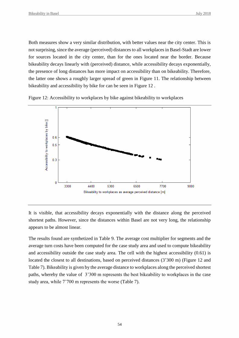
Bikeability in Basel July 2018
54
Both measures show a very similar distribution, with better values near the city center. This is
not surprising, since the average (perceived) distances to all workplaces in Basel-Stadt are lower
for sources located in the city center, than for the ones located near the border. Because
bikeability decays linearly with (perceived) distance, while accessibility decays exponentially,
the presence of long distances has more impact on accessibility than on bikeability. Therefore,
the latter one shows a roughly larger spread of green in Figure 11. The relationship between
bikeability and accessibility by bike for can be seen in Figure 12 .
Figure 12: Accessibility to workplaces by bike against bikeability to workplaces
It is visible, that accessibility decays exponentially with the distance along the perceived
shortest paths. However, since the distances within Basel are not very long, the relationship
appears to be almost linear.
The results found are synthetized in Table 9. The average cost multiplier for segments and the
average turn costs have been computed for the case study area and used to compute bikeability
and accessibility outside the case study area. The cell with the highest accessibility (0.61) is
located the closest to all destinations, based on perceived distances (3’300 m) (Figure 12 and
Table 7). Bikeability is given by the average distance to workplaces along the perceived shortest
paths, whereby the value of 3’300 m represents the best bikeability to workplaces in the case
study area, while 7’700 m represents the worse (Table 7).

Bikeability in Basel July 2018
55
Table 9: Synthesis results of Bikeability and accessibility by bike
Minimum value for
all destinations
Average value for
all destinations
Maximum value for
all destinations
Average distance along the perceived
shortest paths [m] 3’300
4’400
7’700
Accessibility to workplaces by bike [ ] 0.31 0.50 0.61
Average cost multiplier segments [ ] 1.34
Average turn cost [m] 72
Source: Own calculations

Bikeability in Basel July 2018
56
5 Findings and recommendations
5.1 Overview
The results presented in section 4.3 show how bikeability- and accessibility to workplaces by
bike is distributed in Basel. The next step is to conduct an analysis that enables us to locate
shortcomings in the network and thus find out where improvements are necessary (section
5.2). A sensitivity analysis will be carried out in order to see how bikeability and accessibility
change due to changes in network (section 0). Afterwards, bikeability and accessibility will be
computed again, this time for only one destination (train station Basel SBB) (section 0). The
next step is to find out which how the cycling quality of segments and intersections influences
bikeability and accessibility by bike (section 5.5). Finally, possible applications of the method
will be discussed (section 5.6).
5.2 Identifying locations where network improvements are necessary
As seen in the results presented in 4.3, the results of both bikeability and accessibility are
strongly influence by the actual distance to destinations. Areas from which workplaces are
easier to reach, automatically show better values, but this does not say much about the quality
of the network. In order to be able to visualize the influence of the cycling quality, and to locate
shortcomings in the network, a new measure is needed.
This measure will rely on the difference between bikeability based on perceived distance and a
computation based on the actual (scaled) distances for each cell in the case study area. The
reasoning is as follows: when cycling quality is not considered, the cost of a cycling trip is
given only by the actual distance from source to destination. In this case, during the cycling
trip, the cumulative cost of the trip increases at constant rate. However, if cycling quality is
included in the calculation, the actual distances are scaled by the cost multipliers of segments
(and they are also increased by the turn costs) to obtain the perceived distance. The cumulative
cost of a trip based on the perceived distance increases at lower rate along segments of high
quality, and at higher rate along segments with lower quality (Figure 13).
Visualizing the differences between the two types of cumulative costs in the network provides
insight into how the cycling quality changes along different routes. In order to do so, it is
necessary to scale the all the actual distances to destinations in the case study area by a factor
(in this case 1.79), so that their average value will be equal to the average perceived distance.
Without the scaling, the actual distances will always be shorter than the perceived distances,

Bikeability in Basel July 2018
57
and the comparison between them is not meaningful. The difference between the two measures
for each cell shows the areas for which the quality of the network is above or below average.
The distances are computed along the shortest (perceived) paths from each source to each
destination. Orange spots surrounded by green indicate places with an average perceived
distance to destinations larger than the average scaled actual distance. These spots indicate poor
connectivity. Their outgoing links towards the green areas are characterized by low quality.
Similarly, for green spots surrounded by yellow, the average perceived distance to destinations
is lower than the scaled actual distance and this spots are well connected to the surrounding
areas. Because orange spots indicate poor connectivity, they indicate places that need
improvements.
Figure 13: The cumulative cost for a cycling trip based on actual distance compared to the
cumulative cost for a cycling trip based on perceived distance
The differences between the average perceived distances to workplaces and the average scaled
actual distances for the case study area can be seen in Figure 14.

Bikeability in Basel July 2018
58
Figure 14: Difference between the average perceived distances to workplaces and the average
scaled real distances for the case study area. Orange spots represent poorly connected areas,
while green spots indicate good connectivity
Therefore, this comparison enables us to identify locations in the network for which
improvements in the network are necessary. The cycling quality maps of segments (Figure 5)
and intersections (Figure 10) show which elements have poor quality, but they do not tell us
where improvements are most relevant. For example, if a cyclists can choose between two
parallel routes that are significantly different in quality but comparable in distance, improving
the route with lower quality does not bring any advantage to the cyclist. However, poor
connected spots (Figure 14) are less reachable than the average, therefore it can be said that
there are no high quality alternative routes from the surrounding areas.
Moreover, this analysis enables us to find out by how much segments and intersections
influence bikeability. In order to scale the actual distances to obtain the same average values as
for perceived distances, a factor of 1.79 is necessary. This has been found out by trying out
different values. The average cost multiplier of segments amounts to 1.34, which is 75% of
1.79. Therefore, the quality of segments has a contribution of 75% to the calculation, while turn
costs contribute by 25%. Therefore, bikeability and accessibility values are influenced more by
changes in the segment quality, than by adjustments in intersection quality. For this reason, the
sensitivity analysis will only consider changes in the attributes of segments.

Bikeability in Basel July 2018
59
5.3 Sensitivity analysis
A sensitivity analysis is carried out to find out how bikeability- and accessibility to workplaces
by bike change if certain attributes are changed. Two scenarios have been carried out, one with
an improved version of the cycling network within the case study area (Scenario Optimization)
and one in which a number of street segments are made unavailable for cyclists (Scenario
Deterioration) (Figure 15). The first scenario is aimed at improving the poorly connected spots
identified in section 5.2. Hereby, 1% of the total street length of the canton of Basel-Stadt is
adjusted using a number of cycling measures. In the second scenario, 100 street segments,
corresponding to 3% of the total street length in the canton are made unavailable for cyclists
within the whole network of Basel-Stadt (Figure 15). The existing situation shown in section
4.3 will be referred to as the Base Scenario.
Figure 15: Scenario Optimization (left) and Scenario Deterioration (right)

Bikeability in Basel July 2018
60
After conducting these changes, bikeability and accessibility to workplaces by bike are
computed again for both scenarios. The new bikeability for both scenarios, as well as the
differences from the base scenario are visualized in Figure 16. To calculate the differences, the
accessibility by bike of the Base Scenario has been subtracted from the accessibility with each
new scenario.
Figure 16: Bikeability to workplaces for Scenario Optimization (left) and Scenario
Deterioration (right) as absolute values (top) and as differences from the Base Scenario
(bottom)

Bikeability in Basel July 2018
61
The changes in of bikebility- and accessibility from the base scenario can be seen in Table 10.
Table 10: Average bikeability- and accessibility to workplaces by bike for the Base Scenario,
Scenario Optimization and Scenario Deterioration
Base Scenario Scenario Optimization Scenario Deterioration
Average accessibility [ ] 0.501 0.506 0.462
Change in average accessibility
from the base scenario [%] - +1 -8
Average Bikeability [m] 4’577 4’507 6’407
Change in average bikeability from
the base scenario [%] - +2 -29
Source: Own calculations
From Figure 16 it appears that the improvements in the network of Scenario Optimization
influence bikeability mainly locally. The areas in the vicinity of the segments show higher
values than the Base Scenario, but the rest of the area shows limited improvement. The average
bikeability for the whole area increases only with 2%, and the average accessibility by 1%
(Table 10). On the other hand, Scenario Deterioration shows a decrease of 29% in bikeability
and of 8% in accessibility, and has a more uniform effect (Figure 16). The larger impact of the
second scenario has to do with the fact that the average actual distances have been decreased
after making the streets unavailable for cyclists. Moreover, the total segment length adjusted in
this scenario is three times higher than in the previous one. Also, many of the segments made
unavailable in the second scenario are located outside the case study area. In Scenario
Optimization, the improved segments are located only in the case study area, and fewer routes
are affected by the changes.
Although the average bikeability- and accessibility by bike show limited improvement in
Scenario Optimization, one can look at the improved locations to see by how much they change.
Therefore, a cell along an improved axis is chosen for analysis. The perceived distances to all
destinations are measured for the Base Scenario and Scenario Optimization (Figure 17).

Bikeability in Basel July 2018
62
Figure 17: Chosen source cell from the case study area (left) and its distribution of perceived
distances for the Base Scenario and Scenario Optimization (right)
It has been found, that the maximum reduction in perceived distance amounts to 881 m (29%
higher bikeability than in the Base Scenario), while the average reduction amounts to 270 m
(3% better than in the base scenario). This improvement in bikeability is rather substantial.
Therefore, although improvements in the network have a limited effect on the case study area
as a whole, their local impact on the nearby locations is quite large.

Bikeability in Basel July 2018
63
5.4 Computing bikeability and accessibility for only one destination
Both bikeability and accessibility to workplaces by bike shown in Figure 11 show a rather
uniform spatial distribution, with the central areas showing better values. The computations are
based on average perceived distances (along the shortest paths) to workplaces. Because each
average value is influenced by all destinations, some of them being located very close and others
very far away, the range of values for both measures is not very wide. Moreover, the chosen
routes are very disperse, and it is hard to see in practice which routes are preferred and why.
For these reasons, it is interesting to find out how bikeability and accessibility by bike will
change if one considers only one destination. In this case, the train station Basel SBB, has been
chosen because it is an important destination for commuter cyclists and provides bicycle
parking. Bikeability- and accessibility by bike to Basel SBB for the case study area is shown in
Figure 18.
Figure 18: Bikeability and accessibility by bike to Basel SBB for the case study area

Bikeability in Basel July 2018
64
It can be clearly seen in Figure 18 that both bikeability and accessibility show better values in
the vicinity of Basel SBB and they decrease with distance. Accessibility decreases faster than
bikeability, because the former one decays exponentially, while the latter one decays linearly
with distance. The difference between the two measures appears to be more pronounced than
when more destinations are included in the calculation. Moreover, both measures decay faster
with distance than when more destinations are present and a much wider spectrum of values for
both values is observed. The reason is that the computation is not based on average values any
more. In the previous computation, the presence of many nearby destinations increases
bikeability and accessibility considerably, while the destinations located further away decrease
them, leading to a narrower spectrum of values. Overall, the average bikeability and
accessibility for the whole study area have decreased compared to the computation in section
4.3 (Table 11). The reason for this is, that nearby destinations are more influential than the ones
located further away when more destinations are considered.
Table 11: Average values for bikeability and accessibility for the computation with
workplaces as destinations and for the one with Basel SBB as destination
Computation using workplaces
as destinations
Computation using Basel SBB
as destination
Average accessibility [ ] 0.501 0.467
Change in average accessibility
from the original computiation [%] - -6
Average Bikeability [m] 4‘577 4‘811
Change in average bikeability from
from the original computiation [%] - -5
Source: Own calculations

Bikeability in Basel July 2018
65
5.5 The influence of segment attributes on sensitivity
As mentioned in section 5.2, it has been found that the quality cost multiplier of segments has
a contribution of 75% to the bikeability score, whereas turn costs contribute by 25%. Therefore,
the attributes of segments have a much higher influence on the quality cost for routes. In order
to see which segment attributes are influential in the calculation, it is necessary to look at the
distribution of costs for each segment attribute separately.
The maps in section 4.1 (Figure 7 - Figure 9) show the spatial distribution of costs for each
attribute. In this section, the distributions of costs among the number of segments are shown in
Figure 19 for the total cost and the separate attributes, except for the riding environment. The
range of costs described as “high quality” indicates that there is no increase in the scaled length
due to them.
Figure 19: Distribution of costs among the segments for the total cost (top left), gradient cost
(top right), cycling infrastructure costs (bottom left) and hazard costs (bottom right)

Bikeability in Basel July 2018
66
Similarly to the findings in section 4.1, we see that the total cost is strongly correlated with the
gradient cost. For both types of costs, 44% of the segments are of high quality. Moreover, we
see that for both the cycling infrastructure and additional hazards, the vast majority of segments
are of high quality. It is important to note that this histograms do not take into account the length
of the segments, nor the spatial distribution of segments within the area. However, by
comparing Figure 5 and Figure 6 in section 4.1 one can also observe a strong correlation
between gradient costs and total costs, while Figure 7 and Figure 8 show that the cycling
infrastructure cost and hazard cost are low for most segments.
In conclusion, one can state that from all the chosen attributes, the gradient has the most
influence on cost multiplier of segments, and therefore also on bikeability. In the planning
practice, changes in gradient are difficult to implement, although bridges for cyclists are a
possibility. This affects the sensitivity of the method: because the gradient has a high influence,
but most measures in practice focus on the cycling infrastructure and the hazards, the total
bikeability score will not change significantly with the new measures. In order quantify the
influence of the gradient on the bikeability score, a sensitivity analysis could be carried out to
see how bikeability changes if all the gradients are made 0. This goes beyond the scope of the
project, but can be a topic for further research (see section 6).
Furthermore, because the cycling infrastructure and the hazards have low costs for most
segments in the case study area, improving a few segments with higher costs is not expected to
significantly impact bikeability, although this depends on the lengths of the segments and on
their position in the network.
5.6 Application in urban planning
The framework developed for this project enables planners not only to assess the quality of
streets and intersections regarding cycling, but also to locate where improvements in the
network are necessary (see section 5.2). An improvement of a low quality street might not be
necessary, if an alternative route provides a better quality without a significant increase in
distance. Moreover, the method can be applied for different types of destinations (see section
0), and can be expanded to consider the needs of different types of cyclists and E-Bikes (see
section 6.1).
Another practical application of the method is to assess the impact of different planning
measures on bikeability. After assessing bikeability for an existing area, one can conduct the
assessment again with the proposed measures to see how it changes (see section 0). Moreover,
one can compare different planning measures to see which one of them has the higher impact
on bikeability. These measures can be directly related to cycling (such as adding a new cycle

Bikeability in Basel July 2018
67
track), but also the effect of other planning measures can be assessed this way (for example
building a new road).
Moreover, the bikeability framework is a useful tool for the cantonal authorities working on the
Cycling Directive Plan, because it can provide insight into which roads are suitable to be
included in the cycling network. Segments of lower quality should not be included, especially
if alternative routes provide better quality without a significant increase in travel distance. By
expanding the method to consider the needs of non-commuter cyclists (see section 6.1) one can
also assess if a road is more suitable as a commuting route, or as a basic route.
Furthermore, the method enables planners and real estate companies to compare neighborhoods
with each other based on their attractiveness for cycling. This way, real estate companies can
find suitable locations for their projects, if they are interested in cyclists as a target group.

Bikeability in Basel July 2018
68
6 Conclusion
The bikeability framework developed in this study provides planners with a powerful tool in
assessing the impact of different planning measures on cycling, as well as identifying relevant
locations that need improvement. The current framework has many advantages compared to
the existing methods of assessing bikeability, but it also has some limitations. However, these
can be addressed by expanding and improving the method, as it will be explained in section
6.1.
6.1 Evaluation of the research method
The main strength of the method lies in the fact that it enables planners to identify relevant
locations for improvement in the cycling quality. Moreover, it relies on a holistic approach
based on the relevant attributes identified and quantified according to literature for both
segments and intersections. Most existing methods to assess bikeability only consider the
quality of segments (Winters et al. (2013); Krenn et al. (2015)). The BLOS method includes
both segments and intersections, but it does not take into account the gradient for segments and
the presence of cycling infrastructure at intersections (Huff & Ligett, 2014). Moreover, these
methods only consider the quality for cycling, but do not provide any insight into which
locations are relevant for improvement and do not enable the quantification of improvements.
Lowry et al. (2012) is the only study found in literature that includes the distance to destinations
in the bikeability calculation, and enable the quantification of improvements.
Furthermore, the method is suitable for various applications in urban planning (see section 5.6).
Although some attributes and values have been selected based on a study conducted in the US
(Broach et al., 2012), the method is applicable in the Swiss context. Many Swiss national norms
and guidelines, as well as the cantonal guidelines of Basel have been used to identify relevant
attributes. Typical attributes for Basel (and other Swiss cities) are the presence of steep
gradients, longitudinal parking, tram tracks, and the use of low speed limits for residential
streets.
Of course, the current analysis has a number of limitations. First of all, it is conducted for a
relatively small case-study area, it considers only commuter cyclists, two types of destinations
(workplaces and the main train station) and does not take into account E-Bikes. Nevertheless,
the method can be applied for other destinations and for larger areas, and can be expanded to
include other types of cyclists and E-Bikes. Expansion and improvements of the method should
focus on the following points:

Bikeability in Basel July 2018
69
1. Select and quantify the segment and intersection attributes based on revealed – or stated
preferences surveys. A revealed preferences study could be conducted by comparing
GPS traces of the actual cycling routes with the shortest routes in order to identify and
quantify the attributes that are important for cyclists in Basel. This method has been
used by Broach et al. (2012), Krenn et al. (2015) and Winters et al. (2013). Although
the values used in the current thesis are taken from the existing route choice model of
Broach et al. (2012), it is important to note that their research has been conducted in US,
and cyclists in Basel might have different expectations (see section 3.8). An alternative
to using GPS traces is to conduct a stated preferences survey, in which cyclists are asked
which attributes are important for them, and how much they would detour from the
shortest route in order to use segment or intersection with the desired attribute.
However, GPS traces are likely to offer a better estimation of the actual values.
2. Expand the method to include the needs of non-commuting cyclists. Because this also
includes safety oriented users, such as children and seniors, higher costs for cycling
infrastructure and for hazards are expected to be necessary (Pestalozzi & Stäheli, 2012).
Moreover, non-commuting cyclists ride for different trip purposes than commuters,
such as leisure cycling. In this case, the riding environment is expected to play a greater
role than for commuting cyclists. As a later step, the analysis aimed for non-commuting
cyclists can be compared with the one for commuters, to see if an area shows different
bikeability levels for both cases.
3. Conduct the analysis for different types of destinations, such residential areas, parks or
commercial destinations and expand the case-study area to the whole city. Bikeability
to parks is mainly relevant for leisure trips.
4. Expand the method to include the needs of E-Bike users. It is expected that positive
gradients (cycling uphill) will not lead to high costs for them. However, the risks
associated with cycling downhill might increase due to the higher speeds of E-Bikes.
More research is needed to see if the cycling infrastructure costs should be different for
E-Bikes. Due to the reduction in physical effort required to cycle, E-Bikers might be
willing to take longer detours from the shortest route in order to use a segment or
intersection with the desired attributes.
5. Refine the quality assessment of segments by including the pedestrian traffic volumes
in the cycling infrastructure cost. The quality assessment of intersections can be refined
by including the crossing distance and the influence of measures regarding specific
traffic lights for cyclists. The bikeability calculation can be refined by considering
destinations outside the cantonal (and national) border. Moreover, destinations located

Bikeability in Basel July 2018
70
very close to the source could be excluded, because very short distances (up to 500 m)
are not expected to be covered by bike.
6. Exclude nearby destinations (up to 300 m), to which people are more likely to walk than
to cycle.
6.2 Further research
The presented work offers opportunity for further research. An important topic is the issue of
stated- and revealed preferences surveys (see section 6.1) that aid refining the choice of
attributes and their quantification. Another topic for further research is the validation of the
current method. This can be done against existing counts of the number of cyclists at certain
locations, or with the aid of a map with the cyclists traces, for example the one of STRAVA
(2018). This way, one can see if the cyclists really use the streets and intersections with higher
cycling quality. However, this comparison must be done with care, because the choice of riding
on a certain street depends also on the actual distance along the cyclist’s route, and not only on
the attributes (see sections 3.2 and 3.8).
Furthermore, further research is needed to quantify the effect of each street and intersection
attribute on bikeability. This can be done by conducting more sensitivity analyses. An example
is to conduct the analysis with a gradient value of 0 for all segments, to see how bikeability
changes. This way, the influence of the gradient on the total bikeability score can be quantified.
Additionally, it is interesting to find out whether there is a relationship between the bikeability
of an area and the modal share of cycling. This could be done by conducting the analysis in
different cities with different modal shares. The comparison between different areas can also
enable transport planners to define target values for bikeability. For example, the bikeability
score of a city with a high modal share of cycling (such as Basel) could serve as a target value
that other cities aim to achieve. Therefore, they must know by how much their bikeability score
must improve in order to achieve a certain modal share for cycling.
Finally, the relationship between network density and bikeability can be an interesting topic for
further research. Areas with a denser network are expected to have better values, because the
actual distances will be shorter, and therefore also the perceived distances will be shorter.
Therefore, by comparing different areas with each other according to their bikeability, one
should also take into account the network density.

Bikeability in Basel July 2018
71
7 References
Agerholm, N., Caspersen, S., Madsen, J. C. O., and Lahrmann, H. (2006) Cykelstiers
trafiksikkerhed - en før-efterundersøgelse af 46 nye cykelstiers sikkerhedsmæssige
effekt. Dansk Vejtidsskrift, 83(12), 52–57.
Arendt, M., D. Marconi, P. Oswald, I. Salzmann, A. Stahel and S. Vogt (2015)
Gesamtverkehrsmodell der Region Basel. Ergebnisse Ausgangszustand und Szenarien
2030, Basel/Liestal.
ARE Office for Spatial Development (2016) Nationales Personen- und Güterverkehrsmodell
des UVEK – DWV/DTV des Personen-, Güter- und Lieferwagenverkehrs, Bern.
ASTRA Swiss Federal Roads Office (2017) Macroscopic modelling of bicycle and pedestrian
travel – foundation, Bern.
ASTRA Swiss Federal Roads Office, SchweizMobil, Fonds für Verkehrssicherheit (2008)
Planung von Velorouten. Handbuch, Bern.
Axhausen, K.W. (2016) Gravity models, Transport Planning Methods, ETH Zürich, Zürich
Baker, J., and M. Schmidt (2017) Planungshilfe für die Gestaltung von Anlagen des Fuss- und
Veloverkehrs. Grundsätze und Projektierung, BVD, Basel.
Buehler, R., and J. Dill (2015) Bikeway Networks: A Review of Effects on Cycling,
Transport Reviews, https://doi.org/10.1080/01441647.2015.1069908.
Buehler, R., and J. Pucher (2012) City Cycling, the MIT Press, London.
Broach, J., J. Dill and J. Gliebe (2012) Where do cyclists ride? A route choice model
developed with revealed preference GPS data, Transportation Research Part A 46
1730–1740.
Buch, T. S., and Jensen, S. U. (2012) Sikkerhedseffekter af tilbagetrukne stopstreger - før-
efter uheldsevaluering af 123 signalregulerede kryds, Trafitec, Copenhagen.
BVB Basler Verkehrsbetriebe (2018) Projektierungsrichtlinien für Infrastrukturanlagen,
BVB, Basel. BVD Department of Construction and Transport Basel-Stadt (2014) Teilrichtplan Velo 2013
des Kantons Basel-Stadt Erläuterungsbericht, Basel.
Carter, D.L.m W.W. Hunter, C.V. Zegeer and J.R. Stewart (2007) Pedestrian and Bicyclist
Intersection Safety Indices, Turner-Fairbank Highway Research Center. Federal
Highway Administration, FHWA-HRT-06-130.

Bikeability in Basel July 2018
72
Caviedes, A., M. Figliozzi, H. Le, F. Liu and W. Feng (2016) What does stress real-world
cyclists?, paper presented at the 95th Annual Meeting of the Transportation Research
Board, Washington DC.
Celis Consult (2014) Håndbog i cykeltrafik en samling af de danske vejregler på
cykelområdet, Celis Consult, Egå
Clark, S. and A. Davies (2009) Identifying and prioritising walking investment through the
PERS audit tool, paper presented at the Walk21 Proceedings, 10th international
conference for walking. 7–9.
CROW (2007) Design Manual for Bicycle Traffic, Ede.
Dill, J. and N. McNeil (2016) Revisiting the Four Types of Cyclists Findings from a National
Survey, Transportation Research Record: Journal of the Transportation Research
Board, 2587 90–99.
Dill, J., C.M. Monsere and N. McNeil (2011) Evaluation of Bike Boxes at Signalized
Intersections, Transportation Research and Education Center (TREC), University of
Portland, Portland.
Erath, A., M.A.B. van Eggermond, S.S. Ordonez and K.W. Axhausen (2016) Introducing the
Pedestrian Accessibility Tool (PAT): open source GIS- based walkability analysis,
ETH Zurich, Zurich.
Garrick, N. W. (2018) Bicycle Facility and Bicycle Network Design, Verkehr III, ETH Zürich,
Zürich.
Geoportal Basel-Stadt (2018a) Maps BS,
http://map.geo.bs.ch/?lang=en&baselayer_ref=Grundkarte%20farbig.
Geoportal Basel-Stadt (2018b) Geodienste, http://www.geo.bs.ch/geodaten/geodienste.html.
Github (2018) Dijkstra Algorithm, https://github.com/mburst/dijkstras-algorithm.
Hansen, W. (1959) How Accessibility Shapes Land Use, Journal of the American Planning
Association 25 73-76.
Hausigke, S. (2018) Entwicklung eines Bewertungsmodells für die Fahrradfreundlichkeit von
Stadtteilen am Beispiel Berlin, Internationales Verkehrswesen, 70 (1) 59-64.
Huff, H. and R. Ligget (2014) The Highway Capacity Manual’s Method for Calculating
Bicycle and Pedestrian Levels of Service: the Ultimate White Paper, University of
California, Los Angeles.
Hunter, W. W. (2000). Evaluation of Innovative Bike-Box Application in Eugene, Oregon.
Transportation Research Record 1705 99-106.

Bikeability in Basel July 2018
73
Jensen, S. U. (2006) Effekter af cykelstier og cykelbaner: Før-og-efter evaluering af
trafiksikkerhed og trafikmængder ved anlæg af ensrettede cykelstier og cykelbaner i
Københavns Kommune, Trafitec, Copenhagen.
Jensen, S. U. (2008) Safety effects of blue cycle crossings: A before-after study. Accident
Analysis & Prevention 40(2) 742-750.
Kanafani (1983) Transport Demand Analysis, McGraw-Hill, New York.
Kidholm Osmann Madsen, T., and H. Lahrmann (2017) Comparison of five bicycle facility
designs in signalized intersections using traffic conflict studies, Transportation
Research Part F, 46 438-450.
Klobucar, M., and J. Fricker (2007) Network Evaluation Tool to Improve Real and Perceived
Bicycle Safety, Transportation Research Record: Journal of the Transportation
Research Board 2031 25-33.
Krenn, J., P. Oja and S. Titze (2015) Development of a Bikeability Index to Assess the
Bicycle-Friendliness of Urban Environments, Open Journal of Civil Engineering, 5
451-459.
Krizek, K.J., N.J. Tilahun and D.M. Levinson (2007) Trails, Lanes or Traffic: Value of
Different Bicycle Facilities Using Adapted Stated Preferences Survey, Transportation
Research part A, 41 287-301.
Landis, B.W., M. Guttenplan, L.B. Crider (2003) Intersection Level of Service for the Bicycle
Through Movement, Transportation Research Record 1828 101-106.
Lowry, M.B. , D. Callister, M. Gresham and B. Moore (2012) Using Bicycle Level of Service
to Assess Community-wide Bikeability, Transportation Research Record 2314 41-48.
Menghini, G., N. Carrasco, N. Schüssler and K.W. Axhausen (2009) Route choice of cyclists:
discrete choice modelling based on GPS-data, Arbeitsberichte Verkehrs- und
Raumplanung, 544, IVT, ETH Zurich, Zurich.
McNeil, N. (2011) Bikeability and the Twenty-Minute Neighborhood: How Infrastructure and
Destinations Influence Bicycle Accessibility, paper presented at the 90th Annual
Meeting of the Transportation Research Board, Washington DC.
Pestalozzi and Stäheli (2012) Technischer Bericht zum Teilrichtplan Basel-Stadt, BVD
Department of Construction and Transport Basel-Stadt, Basel.
Planungsbüro Jud (2017) Städtevergleich Mobilität. Vergleichende Betrachtung der Städte
Basel, Bern, Luzern, St.Gallen, Winterthur und Zürich im Jahr 2015, Basel-Stadt,
Mobilität, Stadt Bern, Verkehrsplanung, Stadt Luzern, Tiefbauamt, Stadt St.Gallen,
Tiefbauamt, Stadt Winterthur, Tiefbauamt, Stadt Zürich, Tiefbauamt, Zurich.

Bikeability in Basel July 2018
74
Saelens, B. E., J. F. Sallis, and L. D. Frank (2003) Environmental correlates of walking and 3
cycling: findings from the transportation, urban design, and planning literatures, The
Annals of Behavioral Medicine, 25, 80–91.
Schüller, H. (2017) Strassenverkehrssicherheit Entwurf Teil1– Netz + Erschliessungsstrassen,
Strassenverkehrssicherheit, ETH Zurich, Zurich.
Sener, I. N., N. Eluru and C. R. Bhat (2009) An analysis of bicycle route choice preferences
in Texas, US. Transportation 36 511–539.
Stackoverflow (2018a) How do I parse a string to a float or int in Python?,
https://stackoverflow.com/questions/379906/how-do-i-parse-a-string-to-a-float-or-int-
in-python.
Stackoverflow (2018b) Creating a dictionary from a csv file?,
https://stackoverflow.com/questions/6740918/creating-a-dictionary-from-a-csv-file.
Stackoverflow (2018c) Dictionaries and Default Values,
https://stackoverflow.com/questions/9358983/dictionaries-and-default-values#.
Stackoverflow (2018d) How to write multiple values into one line in a text file,
https://stackoverflow.com/questions/6931183/how-to-write-multiple-values-into-one-
line-in-a-text-file.
Stackoverflow (2018e) Iterating over dictionaries using 'for' loops
https://stackoverflow.com/questions/3294889/iterating-over-dictionaries-using-for-
loops.
Stackoverflow (2018f) Read CSV items with column name,
https://stackoverflow.com/questions/41567508/read-csv-items-with-column-name.
Stackoverflow (2018g) Skipping Iterations in Python,
https://stackoverflow.com/questions/549674/skipping-iterations-in-python.
STRAVA (2018) Global Heatmap for Cycling,
https://www.strava.com/heatmap#12.95/7.58925/47.55787/hot/ride.
Strickler, J. (2014) Using defaultdict in Python, https://www.accelebrate.com/blog/using-
defaultdict-python/.
Swiss Confederation (2017) Bundesgesetz über die Beseitigung von Benachteiligungen von
Menschen mit Behinderungen, https://www.admin.ch/opc/de/classified-
compilation/20002658/index.html.

Bikeability in Basel July 2018
75
Swisstopo (2018a) Map of Accidents Involving a bicycle,
https://map.geo.admin.ch/?lang=en&topic=ech&bgLayer=ch.swisstopo.pixelkarte-
farbe&layers=ch.swisstopo.zeitreihen,ch.bfs.gebaeude_wohnungs_register,ch.bav.halt
estellen-oev,ch.swisstopo.swisstlm3d-wanderwege,ch.astra.unfaelle-
personenschaeden_fahrraeder&layers_visibility=false,false,false,false,true&layers_tim
estamp=18641231,,,,99990101.
Swisstopo (2018b) Background Map,
https://map.geo.admin.ch/?lang=en&topic=ech&bgLayer=ch.swisstopo.pixelkarte-
grau&layers=ch.swisstopo.zeitreihen,ch.bfs.gebaeude_wohnungs_register,ch.bav.halte
stellen-oev,ch.swisstopo.swisstlm3d-wanderwege,ch.astra.unfaelle-
personenschaeden_fahrraeder,ch.bfs.volkszaehlung-
gebaeudestatistik_gebaeude&layers_visibility=false,false,false,false,false,false&layers
_timestamp=18641231,,,,99990101,2016&E=2611197.61&N=1268681.18&zoom=6
Swisstopo (2018c) swissALTI3D,
https://shop.swisstopo.admin.ch/en/products/height_models/alti3D.
TBA Department of Civil-Engineering Basel-Stadt (2018), GeoViewer TBA, https://tba-
bs.ch/geoviewer/.
TRB Transport Research Board (2000) Highway Capacity Manual, the National Academy of
Science, Washington.
The Office of Mobility Basel-Stadt (2018a) Velo, http://www.mobilitaet.bs.ch/velo.html,
Basel.
The Office of Mobility Basel-Stadt (2018b) Pilotversuche,
http://www.mobilitaet.bs.ch/velo/pilotversuch.html, Basel.
The Office of Mobility Basel-Stadt (2018c) Teilrichtplan Velo
http://www.mobilitaet.bs.ch/velo/veloverbindungen/teilrichtplan-velo.html
The Office of Mobility Basel-Stadt (2018d) Strassennetzhierarchie
http://www.mobilitaet.bs.ch/motorfahrzeuge/strassennetz/strassennetzhierarchie.html
VSS Swiss Association of Road and Traffic Professionals (2017) SN 640 252: Knoten
Führung des Veloverkehrs, Zurich.
VSS Swiss Association of Road and Traffic Professionals (1999) SN 640 262: Knoten,
Knoten in einer Ebene (ohne Kreisverkehr), Zürich
VSS Swiss Association of Road and Traffic Professionals (1994) SN 640 060 Leichter
Zweiradverkehr, Grundlagen, Zürich
Walk Score (2015) Walk Score Methodology, https://www.walkscore.com/
methodology.shtml.

Bikeability in Basel July 2018
76
Walter, U. (2017a) Anlagenentwurf Veloverkehr, Fuss und Veloverkehr, ETH Zurich, Zurich.
Walter, U. (2017b) Aufbau von Veloverkehrsnetzen, Fuss und Veloverkehr, ETH Zurich,
Zurich.
Winter, S. and Grunbacher A. (2002) Modeling Costs of Turns in Route Planning, Institute for
Geoinformation Technical University Vienna, Vienna.
Winters, M., E.M. Setton, K. Teschke and M. Brauer (2013) Mapping bikeability: a spatial
tool to support sustainable travel, Environment and Planning B: Planning and Design
40 865 – 883.
WolframAlpha (2018), Online Equation Solver,
http://www.wolframalpha.com/calculators/equation-solver/.

Bikeability in Basel July 2018
77
A Additional information regarding methodology
A.1 Case study Basel
A.1.1 The Cycling Directive Plan and the Cycling Network of Basel-Stadt
The Cycling Directive Plan of Basel-Stadt is a cantonal planning instrument and is binding for
the communal and cantonal authorities. It concerns itself with planned changes in the cycling
network and consists of a network map of the changes within the existing network, and a
report in which these changes are explained within the planning context. The network map is
shown in Figure 20. It is distinguished between commuting- and basic routes: The former
ones (shown in blue) are intended mainly for experienced cyclists, for which directness is the
main priority. The latter ones (shown in red) are for cyclists with increased safety needs, such
as seniors and children. For these routes, a higher level of safety is aimed for in the planning
and design process, compared to commuting routes.
Figure 20: Network map of the Cycling Directive Plan of Canton Basel-Stadt. Commuting
routes are shown in blue, basic routes are shown in red. Source: The Office of Mobility Basel-
Stadt (2014)
Source: The Office of Mobility Basel-Stadt (2018c)

Bikeability in Basel July 2018
78
A.1.2 The Street Network of Canton Basel-Stadt
The street network of Canton Basel-Stadt consists of residential- and traffic oriented streets.
The former ones are intended for accessing the buildings by car and are not intended for high
motorized traffic volumes or high speeds. The latter ones are meant to enable a proper
circulation of motorized traffic and are usually characterized by high traffic volumes and
higher speed limits. The traffic oriented streets are further classified into motorways, main
connection roads and main collection streets. These are shown in color in Figure 21.
Figure 21: Traffic oriented streets in Basel-Stadt, classified into motorways (yellow), main
connection roads (red) and main collection streets (green)
Source: The Office of Mobility Basel-Stadt (2018d)

Bikeability in Basel July 2018
79
A.1.3 Map of important locations in the case study area
Figure 22: Map of the streets and intersections mentioned in sections 4.1 and 4.2.
Intersections are marked with the sign “-“ between the names of the streets
Source: adopted from Swisstopo (2018b)
A.2 Using the dependency between cyclists’ speed and gradient to determine the gradient cost function
In section 3.3 the choice of the gradient cost function is explained. The function is determined
by first choosing three points and then connecting them with the corresponding quadratic curve.
The points (0%,0), (-4%,0), (2%,0.5) have been chosen. The choice of the last point is explained
in this section.
Figure 23 shows the relationship between the cyclists’ speed and the gradient for main roads
(shown as a), as well as for residential streets and separate tracks (shown as b). The separate
tracks include cycle tracks and paths where cyclists ride together with pedestrians (VSS, 1994).
Because most of segments in the cycling network are either residential streets or separate tracks
(see Figure 20 and Figure 21), case b is chosen for the calculation. It appears, that on an uphill
road with an inclination of 2%, the cyclist’s speed amounts to two thirds of his or her original
speed on a flat road, assuming the same amount of physical effort. Therefore, for this gradient,
a person can only cover two thirds of the distance he or she would cover on a flat terrain, with
the same physical effort. In other words, the distance covered along a flat road is 50% longer
than the one covered on an uphill gradient of 2%. Therefore, the perceived distance increases

Bikeability in Basel July 2018
80
with 50% for a gradient of 2%, in comparison to gradient of 0%., so an uphill gradient of 2%
must have a cost of 0.5.
Figure 23: Design speed (y-axis) vs. longitudinal gradient (x-axis). Speed 0 represents the
speed of cyclist on a flat surface.
Source: adopted from VSS (1994), p 8.
A.3 Comparison between Swiss, Dutch, and Danish guidelines regarding the types of cycling infrastructure
The type of cycling infrastructure to be used depends on motorized traffic volumes and speed
limits. However, in different countries there are different norms, guidelines and
recommendations. As explained in section 3.3, the cost function of the cycling infrastructure
has been chosen from the Swiss recommendations and the values found in the route choice
model conducted in US by Broach et al. (2012). It is interesting, however to look at the
guidelines and recommendations from countries with higher modal share for cycling, such as
the Netherlands and Denmark. Table 12 shows the types of cycling infrastructure

Bikeability in Basel July 2018
81
recommended for different speeds and different motorized traffic volumes (AADT) for
Switzerland, Netherlands and Denmark.
Table 12: Comparison between Swiss, Dutch and Danish guidelines and recommendations
Swiss guidelines and recommendations
Speed limit
(Km/h)
AADT
0 – 3’000 veh./day
AADT
3’000 - 10’000 veh./day
AADT
≥ 10’000 veh./day
0 Bikes + pedestrians
Cycle track
- -
10-20 Bikes + motorized + pedestrians - -
30 Bikes + motorized
Bike boulevard
Bike lane / Bus lane Cycle track
Bikes + pedestrians
40 Bike lane / Bus lane Bike lane / Bus lane Cycle track
Bikes + pedestrians
≥ 50 Bike lane / Bus lane Bike lane / Bus lane
Cycle track
Bikes + pedestrians
Cycle track
Bikes + pedestrians
Dutch guidelines and recommendations
Speed limit
(Km/h)
AADT
0 – 3’000 veh./day
AADT
3’000 - 4’000 veh./day
AADT
≥ 4’000 veh./day
0 Bikes + pedestrians
Cycle track
- -
10 - 20 Bikes + motorized + pedestrians - -
30 Bikes + motorized Bikes + motorized Bike lane
Cycle track
40-50 Bike lane
Cycle track
Bike lane
Cycle track
Bike lane
Cycle track
60 Bike lane
Cycle track
Cycle track Cycle track
≥ 70 Cycle track Cycle track Cycle track
Danish guidelines and recommendations
Speed limit
(Km/h)
AADT
0 – 2’500 veh./day
AADT
2’500 - 6’500 veh./day
AADT
≥ 6’500 veh./day
0 - 20 Bikes + motorized - -
30 Bikes + motorized Bike lane Cycle track
40 Bikes + motorized
Bike lane
Bike lane Cycle track
50 Bike lane Bike lane
Cycle track
Cycle track
≥ 60 Bike lane with continuous
margin
Cycle track with physical
separation
Bike lane with continuous
margin
Cycle track with physical
separation
Cycle track with physical
separation
Sources: ASTRA et al. (2008), 31-32. CROW (2007) from Buehler & Pucher (2012) 110, Celis Consult (2014), 23.

Bikeability in Basel July 2018
82
It appears that for all three countries, by speed limits of 50 Km/h it is recommended to use
bike lanes, instead of allowing the cyclists to ride together with cars. For all three countries,
cycle tracks are preferred by higher motorized traffic volumes. However, it becomes clear that
the Dutch and Danish recommend cycle tracks by lower traffic volumes and speeds than the
Swiss. Moreover, in Switzerland it is more common to use mixed traffic between bikes and
pedestrians, while in the Netherlands and in Denmark it is not such a common practice.
A.4 Comparison between the chosen gradient cost function, and the cost function found by Broach et al. (2012)
Figure 24 shows a comparison between the chosen gradient cost function in this study and the
gradient cost found by Broach et al. (2012). It can be seen, that the values are comparable for
positive gradients, while negative gradients have not been found to be influential by them.
Figure 24: Comparison between the chosen gradient cost function, and the gradient cost
determined in the route choice model by Broach et al. (2012)
Source: red graph adopted from Broach et al. (2012)

Bikeability in Basel July 2018
83
A.5 Comparison between the chosen cycling infrastructure cost functions, and the cost function found by Broach et al. (2012)
As explained in section 3.3 the growth of the cycling infrastructure cost for the case Bike +
motorized at 30 Km/h is determined by two points (15’000, 1.2) and (25’000, 2.5) based on the
findings of Broach et al. (2012). However, it is important to note that Broach et al. (2012) do
not use a continuous function, but one based on constant intervals (Figure 25). Most of the time,
their values lie between the cost functions “Bike + motorized at 30 Km/h” and “Bike +
motorized at 50 Km/h” (Figure 25).
Figure 25: Comparison between the chosen cycling infrastructure cost functions, and the cost
function determined in the route choice model by Broach et al. (2012) for cycling together
with motorized transportation
Source: red graph adopted from Broach et al. (2012)

Bikeability in Basel July 2018
84
A.6 Example of a roundabout cost calculation
Roundabouts have not been included as a separate category of intersection in the calculation.
However, they are problematic for cyclists and it is thus important that they lead to a high
increase in cost for cyclists passing through the roundabout. Each approach of the roundabout
is treated as a separate turn. Therefore, each cyclist will take at least two turns while passing
through the roundabout. The total cost of passing through the roundabout will be given by the
sum of all turn costs on all approaches on the cyclist’s route. An example is shown in Figure
26.
Figure 26: Example of cycling trajectory through a roundabout
It is assumed that the motorized traffic volume for each approach (for each incoming and
outgoing segment) amounts to 5’000 veh./day. Because roundabouts are unsignalized (there is
no traffic light) the cost of each approach is given by the Basic turn (67 m) and a traffic cost for
each turn direction (0 m for right turns, 66 m for goings straight) (see Table 4 and Table 5). In
the example in Figure 26 the cyclist will turn right two times (to enter and exit the roundabout)
and will go straight one time, to cross one street. The right turn costs will be equal to 66 m for
each of the two right turns, while the cost of going crossing the other street is equal to 133 m.
Therefore, the total cost of passing through the roundabout is equal to 267 m. This is quite
substantial, since the average turn cost in the case study area is equal to 72 m. Moreover, if each
street has a motorized traffic volume of 10’000 veh./day, the cost of going through this
roundabout will amount to 417 m (see Table 4 and Table 5) which is very high.

Bikeability in Basel July 2018
85
B Additional information regarding spatial data
B.1 The street network
The network of streets has been provided by the Office of Mobility of Basel-Stadt. It contains
all streets and cycle tracks in the canton, represented as segments. A number of attributes is
defined for each segment. For the segments included in the cycling network, data for a number
of attributes has been collected by the canton (see Table 13). For the streets outside of the
cycling network, only the speed limits and the street network hierarchy have been given.
Each segment in the cycling network is defined by a continuous type of cycling infrastructure.
For example, if a bike lane changes to bus lane, a new segment is defined. New segments are
defined at intersections. Moreover, each segment is assigned a predefined direction of travel,
so that attributes can be collected for both directions. This direction can be visualized in GIS.
Fields with attributes along the predefined direction of travel are described with “DR”, while
attributes in the opposite direction are represented with “GDR” or “GD”.
A number of attributes of both segments and intersections have been added in the original
segment layer, to be used for the project. A short description of the attributes used in the
calculation (both the original and the ones added for this project) is shown in Table 13. This
includes the intersection attributes (see appendix C.3). The annotation “Original” under
“Remark” means the field attribute with its corresponding data has been provided by the Office
of Mobility Basel-Stadt. “Added” means it has been assigned later for this project. The
motorized traffic volumes have been collected from the Traffic Model of Region Basel (Arendt
et al., 2015), while the other attributes have been collected from the Geoviewer Map of the
Department of Civil Engineering Basel-Stadt (2018).

Bikeability in Basel July 2018
86
Table 13: Description of the important fields in the segment layer (including intersections)
Field name Explanation Remark
Art_DR, Art_GDR Type of cycling infrastructure in each direction Original
Breite_DR, Breite _GDR Width of cycling infrastructure in each direction Original
Geschw Speed limit Original
StrnetzHr Street network hierarchy (HLS, HVS, HSS or NULL) Original
SHAPE_Leng Segment length Original
KapHst_DR, KapHst_GDR Tram stop along the sidewalks Original
NutzNeb_DR, NutzNeb_GD Additional uses (longitudinal / angular parking) Original
newid Segment ID Added
knot_0 Intersection ID of the starting point of the segment Added
knot_1 Intersection ID of the ending point of the segment Added
x_0, y_0 Coordinates of the starting point of the segment Added
x_1, y_1 Coordinates of the end point of the segment Added
DWV Weekly motorized traffic volumes Added
Str_br Street width Added
TR_V_L Heavy traffic > 8% (for traffic oriented streets) Added
Slope Gradient Added
Velostrass Bike boulevard Added
Green_mean Average of green and aquatic area within the buffer Added
area Segment within the case study area Added
LT_BR_DR, LT_BR_GD Insufficient space between tram tracks and parking Added
BL_PP_DR, BL_PP_GD Insufficient space between bike lane and parking Added
Angle_star, Angle_end Angle between each end of the segment and the vertical axis Added
dr_priorit, gdr_priori Priority at unsignalized intersection Added
dr_infr_l, gdr_infr_l Presence of bike lane for going left Added
dr_infr_s, gdr_infr_s Presence of bike lane for going straight Added
dr_rc, gdr_rc Presence of a car lane turning right Added
dr_lanes, gdr_lanes Number of car lanes Added
dr_bb, gdr_bb Presence of bike box Added
Source: Own description of the data regarding the segment layer provided by the Office of Mobility

Bikeability in Basel July 2018
87
B.2 Workspaces
Data regarding workspaces have been provided by the Office of Mobility as a point layer in
GIS. Each point describes the center of each hectare in the canton with the number of employees
in the hectare. Missing points represent places with no workspaces. The original fields used are
“Objectid” (the ID of each point) and “emptot” (total number of workspaces in the hectare).
Additionally, the field “TargetID” represents the ID of the closest intersection, calculated with
the distance matrix, which is used in the computation of the shortest perceived path (see
appendices C.5 and C.5).
C Additional information regarding calculations
C.1 Computing the gradient
The gradient has been calculated by using raster data with altitudes from Swisstopo (2018),
with a precision of 1 m. The ends of the street segments have been buffered with 5 m and the
average height within this buffer has been calculated. Based on this heights, the gradient for
each segment has been computed using the open field calculator. However, the raster image
only contains altitudes based on the natural environment, and buildings are not included.
Therefore, in the vicinity of bridges and tunnels, the gradient must be manually adjusted. This
is done by using the gradient tool of the Geoviewer map of TBA (2018), which accounts for
inclinations due to the built environment.
C.2 Computing the coverage of green and water
GIS vector data with trees (as lines) as well as shrubs and grass (as polygons) is provided by
the cantonal administration (Geoportal Basel-Stadt, 2018b). The tree lines have been buffered
(with 10 m) to approximate the green coverage of trees. Then the data have been converted to
raster by saving the GIS file as image and has been imported back in QGIS. The street
segments have been buffered with 20 m, in order to include only the green and aquatic areas
that are in the proximity of the street. This way, green areas located behind buildings are not
included. A colour code has been used in order to calculate the percentage using the “mean”
function of the tool “Zonal Stats”. The green- and aquatic areas have received a colour of
RGB code of (0,0,0), while the background has been assigned the colour with RGB
(100,100,100). This way, by calculating the mean between the colors (0,0,0) and
(100,100,100) the result is automatically expressed as percentage. It represents the percentage
of green and aquatic areas within the buffer.

Bikeability in Basel July 2018
88
C.3 Generating intersections and annotating segments with intersection IDs
It is important that the intersection data and the ones of the segment data are found in the same
layer, in carry out the calculation with the python console. Therefore, data regarding attributes
of intersections will be collected in the same layer as the segments.
In order to generate the intersections, the coordinates of the segment ends have been extracted
using the tools xat and yat in the Open field calculator. Afterwards, the segment layer has been
exported as a CSV and imported in Excel. Here, the ends of the segments have been grouped
in Excel according to their coordinates and have been given an ID (knotid) as an ID of the
intersection. Then, the intersections have been imported in QGIS as a point layer and used for
visualization. The same Excel file has been used to generate the ids of the intersections at the
ends of the segments, denoted as knot0 and knot1. As explained in appendix B.1 each segment
has a predefined direction denoted as DR, which corresponds to the direction from knot0 to
knot1. Similarly, direction GDR (opposite to the predefined direction) corresponds to the
direction from knot1 to knot0.
The intersection attributes are added as new columns. The ones starting with prefix “dr”
correspond to knot1, and while the prefix “gdr” corresponds to knot0. In order to know if the
data must be collected for the fields with prefix “dr” or for the ones starting with “gdr”, one
needs to look at the knotid from the point layer. If the field knot1 from the segment layer
corresponds to knotid in the point layer, the data will be collected for “dr”. Similarly, if knot0
corresponds to knotid, the data will be collected for the fields starting with “gdr”.
C.4 Cost calculation for segments and intersections
This section comprises the code to calculate the costs of segments and intersections (including
lengths of segments). The code has been written in the Python Console of QGIS. The reason
for using Python is that a customized solution is needed, to take into account turn costs, segment
attributes and to use them to compute the shortest perceived path with the Dijkstra algorithm.
The Dijkstra algorithm has been computed with a separate code than the segment- and turn cost
(see appendix C.5). Stack Overflow (2018) and Strickler (2014) have been used as an aid for
programming.
It is important to mention, that the requirements regarding cycle track widths explained in
section 3.3 refer to the situation when two cyclists can ride next to each other or in opposite
direction. Because the widths have been collected separately for each half of the track, the
standard widths shown in Table 2 must be divided by 2 in the calculation. Moreover, for bike

Bikeability in Basel July 2018
89
lane widths between 1.2 - 1.5 the cycling infrastructure cost is calculated as a weighted average
between the bike lane width function and the one for the case “bike + motorized” (see section
3.3). This can be written formally as:
𝐶 𝐼𝑛𝑓 = 𝑊𝑓 × 𝐶 𝑏𝑙 + (1 − 𝑊𝑓) × 𝐶 𝑏𝑚 1.2 𝑚 ≤ 𝑊𝑖𝑏𝑙 < 1.5 𝑚,
where 𝐶 𝐼𝑛𝑓 is the cycling infrastructure cost, 𝑊𝑓 is a weighting factor between 0 and 1, 𝐶 𝑏𝑙 and
𝐶 𝑏𝑚 are the cycling infrastructure costs calculated with the cost functions for bike lanes and
“bike + motorized” respectively, and 𝑊𝑖𝑏𝑙 is the width of the bike lane. The cycling
infrastructure cost must be equal to 𝐶 𝑏𝑚 for a width of 1.2 m, and equal to 𝐶 𝑏𝑙 for a width of
1.5 m. Therefore, 𝑊𝑓 must be equal to 0 for a width of 1.2 m and to 1 for a width of 1.5 m. 𝑊𝑓
will be described by the following linear equation:
𝑊𝑓 = 3.333 × (𝑊𝑖𝑏𝑙 − 1.2)
This function of the weighting factor based on the bike lane width is shown in Figure 27.
Figure 27: Weighting factor for the cycling infrastructure costs against bike lane widths
between 1.2 m and 1.5 m
As explained in section 3.6, the center point of each hectare in the case study area is considered
a source and each workplace in Basel (also represented as hectare center point) is considered a
destination for the cyclist’s journey. It is necessary to associate network elements to these
sources and destinations, because the routing calculation can only take place along segments
and intersections. Therefore, the closest intersection to each hectare center point will be
considered a source or a destination in the Dijkstra computation of the shortest path.
Moreover, it is necessary to define virtual points at each intersection, so that the routing can
take place along any segment starting or ending at the intersection. Point “H” has been defined

Bikeability in Basel July 2018
90
as a starting node, from which virtual segments of length 0 lead to the starting points of
segments. Similarly, point “J” is an end node, to which virtual segments of length 0 arrive from
the end points of all segments (see Figure 28). The starting points of the actual segments are
described with “s” as starting points and “e” as ending points, while “d” and “g” account for
the predefined direction of the segment (DR vs GDR) (see Figure 28).
Figure 28: Assigning virtual starting- and ending nodes at each intersection, with virtual
segments of lengths 0 m
Following the recommendations of Winter & Grunbacher (2002) the turn costs have been
defined as virtual lengths that will be added as costs in the Dijkstra algorithm computation
described in appendix C.5. The direction of the turn (left, straight or right) is measured by an
angle between the incoming street and the outgoing street. A value smaller than 160⁰,
represents a right turn, one between 160⁰ and 200⁰ indicates going straight, while an angle
greater than 200⁰ represents a left turn.
The intersections are generated with from the segment ends, but not all segments in the
network end with intersections. For example, when a bike lane changes to bus lane, a new
segment is defined. Therefore, some “fake” intersections are generated, consisting of two
segments. For this reason, a new column called “num_streets” has been defined, which tells
us, for each intersection how many street segments come together. If the value is equal to 2, a
turn cost of 0 is assigned.
The Python code for computing the segment and intersection cost is shown here with
explanations:

Bikeability in Basel July 2018
91
import csv
import types
from collections import defaultdict
from math import exp
# SEGMENT COSTS
# Defining the segment cost functions
def slopecost(slope):
return 417 * slope * (slope + 0.04)
def bike_cars_ped(traffic):
return 1
def bike_cars_30_cost(traffic):
return (0.0110012 * (exp(0.00019686 * traffic))) + 0.988988
def bike_cars_50_cost(traffic):
return (0.0110012 * (exp(0.00025 * traffic))) + 1.28
def bike_lane_30_cost(traffic):
return (0.0110012 * (exp(0.00015 * traffic))) + 0.788988
def bike_lane_50_cost(traffic):
return (0.0110012 * (exp(0.00019686 * traffic))) + 0.988988
def green_water_benefit(greenwater):
return 0.1 - 0.1 / (0.01 + exp(0.05 * greenwater))
# Account for the widths of bike lanes and cycle tracks
def bike_lane_availability(b_width, infra):
if infra == 'Velostreifen':
if b_width < 1.2:
return 0
elif b_width < 1.5:
return 3.333 * (b_width - 1.2)
elif b_width < 1.8:
return 1
else:
return 1.2
elif infra == 'Busspur mit Velozulassung':
return 1 == 'Busspur mit Velozulassung'
elif infra == 'ohne Velomassnahmen' or infra == '' or infra == \
'Einbahnstrasse mit Gegenverkehr':
return 0
def bike_track_cost(b_width, infra):
if infra == 'Veloweg Ein-Richtgung':
if b_width < 1.3:
return 1
elif b_width < 1.5:
return 0.9
else:
return 0.8
else:
if b_width < 1.4:
return 1
elif b_width < 1.7:
return 0.9
else:
return 0.8

Bikeability in Basel July 2018
92
def suitability_seg(
traffic,
infra,
b_width,
speed,
street,
s_width,
Tr_width,
trucks,
pp_bikelane,
slope,
kap_halt,
v_strasse,
greenwater,
len,
use):
# Exclude gradients smaller than -10% and greater than 10%
if slope > 0.1:
slope = 0.1
elif slope < -0.1:
slope = -0.1
# Convert motorized traffic volumes from averages for the working days to
# weekly averages
traffic = 0.9 * traffic
# Include bike boulevards
if v_strasse == 1:
infra_cost = 0.9
# Assign cost for cycle tracks, bike + pedestrians, cycle ban
elif infra == 'Veloweg Ein-Richtgung' or infra == 'Veloweg Gegenverkehr':
infra_cost = bike_track_cost(b_width, infra)
elif infra == 'Fussweg mit Velozulassung' or infra == 'Veloweg mit ' \
'Fussverkehr' or \
infra == 'Fussgaengerzone':
infra_cost = 1
elif infra == 'Fahrverbot':
infra_cost = 5
# define weighted average between the cases Bike + motorized and bike
# lanes (bike lane widths between 1.2 and 1.5 m)
else:
ba = bike_lane_availability(b_width, infra)
if speed <= 20:
infra_cost = bike_cars_ped(traffic)
elif ba > 1:
infra_cost = 1
elif speed <= 30:
cost_bl = bike_lane_30_cost(traffic)
cost_b_cars = bike_cars_30_cost(traffic)
infra_cost = ba * cost_bl + (1 - ba) * cost_b_cars
else:
cost_bl = bike_lane_50_cost(traffic)
cost_b_cars = bike_cars_50_cost(traffic)
infra_cost = ba * cost_bl + (1 - ba) * cost_b_cars
# define costs for additional hazards
if kap_halt == 'vor der Kaphaltestelle':
risk_kap_halt = 0.2
else:
risk_kap_halt = 0
if Tr_width <= 2.65:
risk_tram = 0.3
else:
risk_tram = 0
if trucks == 1 and (street == 'HVS' or street == 'HSS' or street == 'HLS'):
risk_trucks = 0.2
else:
risk_trucks = 0

Bikeability in Basel July 2018
93
if pp_bikelane == 1:
risk_pp_bikelane = 0.2
else:
risk_pp_bikelane = 0
if use == 'Schrägparkierung Auto':
risk_ang_parking = 0.2
else:
risk_ang_parking = 0
if (((s_width <= 5 and traffic >= 2500)
or (s_width <= 6 and traffic >= 5000)
or (s_width <= 7 and traffic >= 7500)
or (s_width <= 7.5 and traffic >= 10000))
and (
infra == 'ohne Velomassnahmen' or infra == '' or infra ==
'Einbahnstrasse mit Gegenverkehr')):
risk_street_width = 0.200
else:
risk_street_width = 0
if Tr_width <= 2.65 and (slope >= 0.04 or slope <= -0.04):
risk_tram_slope = 0.5
else:
risk_tram_slope = 0
if (
slope >= 0.04 or slope <= -0.04) and use == 'Längsparkierung ' \
'Auto' and (
infra == 'ohne Velomassnahmen' or infra == '' or infra ==
'Einbahnstrasse mit Gegenverkehr'):
risk_parking_slope_mix = 0.3
else:
risk_parking_slope_mix = 0
if (Tr_width <= 2.65) and (use == 'Längsparkierung Auto'):
risk_tram_parking = 0.5
else:
risk_tram_parking = 0
if (slope >= 0.04 or slope <= -0.04) and pp_bikelane == 1:
risk_parking_slope_blane = 0.3
else:
risk_parking_slope_blane = 0
# define hazard cost as a maximum of all hazard costs on each segment
risk_total_cost = max(risk_kap_halt, risk_tram, risk_trucks,
risk_pp_bikelane, risk_ang_parking, risk_street_width,
risk_tram_slope,
risk_parking_slope_mix, risk_parking_slope_blane,
risk_tram_parking)
# compute total cost as a sum of the separate attribute costs
cost = infra_cost - green_water_benefit(greenwater) + slopecost(
slope) + risk_total_cost
# exclude costs that are greater than 10 (they are equated with 10)
if cost > 10:
cost = 10
return (infra_cost, green_water_benefit(greenwater), slopecost(slope),
risk_total_cost, cost, cost * len)
# ===================================================================
# TURN COSTS
# define traffic cost for unsignalized turns for each turn direction
def traffic_cost_left(s):
# Convert motorized traffic volumes from averages for the working days
# to weekly averages
s = 0.9 * s
if s <= 5000:
return 0
elif s <= 10000:
return 66
elif s <= 20000:

Bikeability in Basel July 2018
94
return 240
else:
return 885
def traffic_cost_straight(s):
# Convert motorized traffic volumes from averages for the working days
# to weekly averages
s = 0.9 * s
if s <= 5000:
return 0
elif s <= 10000:
return 66
elif s <= 20000:
return 94
else:
return 515
def traffic_cost_right(s):
# Convert motorized traffic volumes from averages for the working days to
# weekly averages
s = 0.9 * s
if s <= 10000:
return 0
else:
return 61
# define turn cost values for each turn cost component
min_turn_cost = 67
res_turn_right = 34
traffic_light_cost = 34
stop_sign_cost = 8
blane_l_dir_B = 0.8
ind_left_turn_B = 0.9
bbox_l_dir_B = 0.7
blane_s_B = 0.9
clane_r_C = 1.1
no_lanes_C = 1.5
# convert to integer or use 0 if the column is empty
def int_or_zero(s):
if s == '':
return 0
else:
return int(s)
def float_or_other(s, other):
if s == '':
return other
else:
try:
return float(s)
except:
print(s)
throw(e)
# convert to float or use 0 if the column is empty
def float_or_zero(s):
return float_or_other(s, 0)
# define dictionary variable which is the list of all the segments for each
# intersection
int_seg = defaultdict(list)
seg = {}
with open(

Bikeability in Basel July 2018
95
'D:\\Master_ETH\\Master_Arbeit\\recalculation_accessibility'
'\\seg_csv_inputs\\seg_orig.csv',
newline='') as csvfile:
reader = csv.DictReader(csvfile, delimiter=',')
for row in reader:
x = types.SimpleNamespace()
x.newid = int(row["newid"])
x.knot_0 = int(row["knot_0"])
x.knot_1 = int(row["knot_1"])
x.network = row["StrnetzHr"]
x.angle_0 = float(row["Angle_star"])
x.angle_1 = float(row["Angle_end"])
x.dr_priorit = row["dr_priorit"]
x.dr_infr_l = row["dr_infr_l"]
x.dr_infr_s = row["dr_infr_s"]
x.dr_rc = int_or_zero(row["dr_rc"])
x.dr_round = int_or_zero(row["dr_round"])
x.dr_lanes = int_or_zero(row["dr_lanes"])
x.dr_bb = int_or_zero(row["dr_bb"])
x.traffic = float_or_zero(row["DWV"])
x.speed = int_or_zero(row["Geschw"])
x.s_width = float_or_zero(row["Str_br"])
x.trucks = int_or_zero(row["TR_V_L"])
x.slope = float(row["Slope"])
x.v_strasse = int_or_zero(row["Velostrass"])
x.greenwater = float_or_zero(row["Green_mean"])
x.len = float(row['SHAPE_Leng'])
x.area = int_or_zero(row["area"])
x.dr_infra = row["Art_DR"]
x.dr_b_width = float_or_zero(row["Breite_DR"])
x.dr_tr_width = float_or_other(row["LT_BR_DR"], 100)
x.dr_pp_bikelane = int_or_zero(row["BL_PP_DR"])
x.dr_kap_halt = row["KapHst_DR"]
x.dr_use = row["NutzNeb_DR"]
x.gdr_infra = row["Art_GDR"]
x.gdr_b_width = float_or_zero(row["Breite_GDR"])
x.gdr_tr_width = float_or_other(row["LT_BR_GD"], 100)
x.gdr_pp_bikelane = int_or_zero(row["BL_PP_GD"])
x.gdr_kap_halt = row["KapHst_GDR"]
x.gdr_use = row["NutzNeb_GD"]
x.gdr_priorit = row["gdr_priori"]
x.gdr_infr_l = row["gdr_infr_l"]
x.gdr_infr_s = row["gdr_infr_s"]
x.gdr_rc = int_or_zero(row["gdr_rc"])
x.gdr_round = int_or_zero(row["gdr_round"])
x.gdr_lanes = int_or_zero(row["gdr_lanes"])
x.gdr_bb = int_or_zero(row["gdr_bb"])
if row["DWV"] == "":
x.dwv = 0
else:
x.dwv = float(row["DWV"])
# put x in a dictionary
seg[x.newid] = x
int_seg[x.knot_0].append(-x.newid)
int_seg[x.knot_1].append(x.newid)
print(int_seg[100])
# writing output file with all turn costs
outputfile = open(
'D:\\Master_ETH\\Master_Arbeit\\recalculation_accessibility'
'\\links_turn_cost_outputs\\seg_turn_orig_cost_detailed.csv',
'w')
outputfile.write('knot_start,knot_end,cost,len,explanation\n')
# writing output file with all segment costs
outputfile_seg = open(
'D:\\Master_ETH\\Master_Arbeit\\recalculation_accessibility'

Bikeability in Basel July 2018
96
'\\links_turn_cost_outputs\\seg_turn_orig_cost.csv',
'w')
outputfile_seg.write(
'newid,infra_cost,green_water_b, slope_cost, risk_total_cost,cost,plen,'
'gd_infra_cost,gd_green_water_b, gd_slope_cost, gd_risk_total_cost,'
'gd_cost, gd_plen\n')
sum_plen = 0
sum_shape_len = 0
sum_turn_cost = 0
count_turns = 0
# iteration over all segments to write segment cost including lenghts of
# segments
for newid in seg:
crt_seg = seg[newid]
dr_infra_cost, dr_green_water, dr_slope_cost, dr_risk_cost, dr_cost, \
dr_plen = suitability_seg(
crt_seg.traffic,
crt_seg.dr_infra,
crt_seg.dr_b_width,
crt_seg.speed,
crt_seg.network,
crt_seg.s_width,
crt_seg.dr_tr_width,
crt_seg.trucks,
crt_seg.dr_pp_bikelane,
crt_seg.slope,
crt_seg.dr_kap_halt,
crt_seg.v_strasse,
crt_seg.greenwater,
crt_seg.len,
crt_seg.dr_use)
explanation = 'segment infra:{} env:{} slope:{} risk:{} multiplier:{' \
'}'.format(
dr_infra_cost, dr_green_water, dr_slope_cost, dr_risk_cost, dr_cost)
# compute segment cost for the area outside the case study area,
# using the average cost multiplier within the case study area (1.35)
if crt_seg.area == 0:
dr_plen = 1.35 * crt_seg.len
explanation = 'outside area'
outputfile.write(
'ds{},de{},{},{},{}\n'.format(newid, newid, dr_plen, crt_seg.len,
explanation))
gdr_infra_cost, gdr_green_water, gdr_slope_cost, gdr_risk_cost, gdr_cost,\
gdr_plen = suitability_seg(
crt_seg.traffic,
crt_seg.gdr_infra,
crt_seg.gdr_b_width,
crt_seg.speed,
crt_seg.network,
crt_seg.s_width,
crt_seg.gdr_tr_width,
crt_seg.trucks,
crt_seg.gdr_pp_bikelane,
-crt_seg.slope,
crt_seg.gdr_kap_halt,
crt_seg.v_strasse,
crt_seg.greenwater,
crt_seg.len,
crt_seg.gdr_use)
explanation = 'segment infra:{} env:{} slope:{} risk:{} multiplier:{' \
'}'.format(
gdr_infra_cost, gdr_green_water, gdr_slope_cost, gdr_risk_cost,
gdr_cost)
if crt_seg.area == 0:
gdr_plen = 1.35 * crt_seg.len
explanation = 'outside area'
outputfile.write(
'gs{},ge{},{},{},{}\n'.format(newid, newid, gdr_plen, crt_seg.len,
explanation))
outputfile_seg.write('{},{},{},{},{},{},{},{},{},{},{},{},{}\n'.format(
newid, dr_infra_cost, dr_green_water, dr_slope_cost, dr_risk_cost,
dr_cost, dr_plen,
gdr_infra_cost, gdr_green_water, gdr_slope_cost, gdr_risk_cost,

Bikeability in Basel July 2018
97
gdr_cost, gdr_plen))
if crt_seg.area == 1:
sum_plen = sum_plen + dr_plen + gdr_plen
sum_shape_len = sum_shape_len + 2 * crt_seg.len
outputfile_seg.close()
for knotid in int_seg:
segment_list = int_seg[knotid]
# sum up traffic volumes in all the segments for each intersection. H is
# a source node withing the intersection, and J is the destination node
# used by Dijkstra
s = 0
num_tr_streets = 0
num_streets = 0
num_area_streets = 0
tl = 0
# define starting nodes to be used by the Dijkstra algorithm
for v in segment_list:
newid = abs(v)
if v < 0:
outputfile.write('H{},ds{},0,0,virtual\n'.format(knotid, newid))
outputfile.write('ds{},J{},0,0,virtual\n'.format(newid, knotid))
else:
outputfile.write('H{},gs{},0,0,virtual\n'.format(knotid, newid))
outputfile.write('gs{},J{},0,0,virtual\n'.format(newid, knotid))
seg_data = seg[abs(v)]
s = s + seg_data.dwv
if v < 0:
priorit = seg_data.gdr_priorit
infr_l = seg_data.gdr_infr_l
infr_s = seg_data.gdr_infr_s
else:
priorit = seg_data.dr_priorit
infr_l = seg_data.dr_infr_l
infr_s = seg_data.dr_infr_s
if seg_data.network != '':
num_tr_streets = num_tr_streets + 1
if seg_data.area == 1:
num_area_streets = 1
num_streets = num_streets + 1
if priorit == 'TL':
tl = 1
# The traffic volume of the intersection is calculated by summing up the
traffic volumes of the incoming- and outgoing streets and dividing by 2
s = s / 2
# define angles between the incoming street and the outgoing street of
# the intersection, to be used for turn direction (right, straight, left)
for entry in segment_list:
min_angle = 99999
max_angle = 0
min_angle_tr = 99999
for exit in segment_list:
if entry == exit:
continue
seg_entry = seg[abs(entry)]
seg_exit = seg[abs(exit)]
if entry < 0:
angle_entry = seg_entry.angle_0
else:
angle_entry = seg_entry.angle_1
if exit < 0:
angle_exit = seg_exit.angle_0
else:
angle_exit = seg_exit.angle_1
rel_angle = angle_entry - angle_exit

Bikeability in Basel July 2018
98
if rel_angle < 0:
rel_angle = rel_angle + 360
if rel_angle < min_angle:
min_angle = rel_angle
if (rel_angle < min_angle_tr) and (seg_exit.network != ''):
min_angle_tr = rel_angle
if rel_angle > max_angle:
max_angle = rel_angle
for exit in segment_list:
if entry == exit:
continue
seg_entry = seg[abs(entry)]
seg_exit = seg[abs(exit)]
if entry < 0:
angle_entry = seg_entry.angle_0
turn_start = 'ge{}'.format(seg_entry.newid)
priorit = seg_entry.gdr_priorit
infr_l = seg_entry.gdr_infr_l
infr_s = seg_entry.gdr_infr_s
rc = seg_entry.gdr_rc
round = seg_entry.gdr_round
n_lanes = seg_entry.gdr_lanes
b_box = seg_entry.gdr_bb
else:
angle_entry = seg_entry.angle_1
turn_start = 'de{}'.format(seg_entry.newid)
priorit = seg_entry.dr_priorit
infr_l = seg_entry.dr_infr_l
infr_s = seg_entry.dr_infr_s
rc = seg_entry.dr_rc
round = seg_entry.dr_round
n_lanes = seg_entry.dr_lanes
b_box = seg_entry.dr_bb
if exit < 0:
angle_exit = seg_exit.angle_0
turn_end = 'ds{}'.format(seg_exit.newid)
else:
angle_exit = seg_exit.angle_1
turn_end = 'gs{}'.format(seg_exit.newid)
rel_angle = angle_entry - angle_exit
if rel_angle < 0:
rel_angle = rel_angle + 360
# define the turn costs for all situations
# define turn cost of 0 for “fake” intersections made up of two segments
if num_streets <= 2:
turn_cost = 0
explanation = 'no intersection'
elif num_tr_streets == 0:
if rel_angle >= 160 and rel_angle <= 200:
turn_cost = 0
explanation = 'residential straight'
elif rel_angle <= 160:
turn_cost = res_turn_right
explanation = 'residential right turn'
else:
turn_cost = min_turn_cost
explanation = 'residential left'
elif tl == 1:
if rel_angle == min_angle:
if infr_s == 0:
turn_cost = min_turn_cost
explanation = 'right turn signalized'
else:
turn_cost = min_turn_cost * blane_s_B
explanation = 'right turn signalized with bike lane'
elif rel_angle == max_angle:
if infr_l == 0:
turn_cost = min_turn_cost + traffic_light_cost

Bikeability in Basel July 2018
99
explanation = 'left turn signalized'
elif infr_l == 1 and b_box == 1:
turn_cost = (
min_turn_cost +
traffic_light_cost) * \
bbox_l_dir_B
explanation = 'left turn signalized with bike box'
elif infr_l == 1 and b_box == 0:
turn_cost = (
min_turn_cost +
traffic_light_cost) * \
blane_l_dir_B
explanation = 'left turn signalized with bike lane'
else:
turn_cost = (
min_turn_cost +
traffic_light_cost) * \
ind_left_turn_B
explanation = 'left turn from residential signalized ' \
'with indirect left turn'
if n_lanes > 2:
turn_cost = turn_cost * no_lanes_C
explanation = explanation + ' 3 lanes'
else:
if infr_s == 0:
turn_cost = min_turn_cost + traffic_light_cost
explanation = 'straight signalized'
else:
turn_cost = (
min_turn_cost +
traffic_light_cost) * blane_s_B
explanation = 'straight signalized with bike lane'
else:
if rel_angle == min_angle:
if infr_s == 0:
turn_cost = min_turn_cost + traffic_cost_right(s)
explanation = 'right turn unsignalized'
else:
turn_cost = (min_turn_cost + traffic_cost_right(
s)) * blane_s_B
explanation = 'right turn unsignalized with bike lane'
elif rel_angle == max_angle:
if infr_l == 0:
turn_cost = min_turn_cost + traffic_cost_left(s)
explanation = 'left turn unsignalized'
elif infr_l == 1 and b_box == 1:
turn_cost = (min_turn_cost + traffic_cost_left(
s)) * bbox_l_dir_B
explanation = 'left turn unsignalized with bike box'
elif infr_l == 1 and b_box == 0:
turn_cost = (min_turn_cost + traffic_cost_left(
s)) * blane_l_dir_B
explanation = 'left turn unsignalized with bike lane'
else:
turn_cost = (min_turn_cost + traffic_cost_left(
s)) * ind_left_turn_B
explanation = 'left turn unsignalized with indirect ' \
'left turn'
if n_lanes > 2:
turn_cost = turn_cost * no_lanes_C
explanation = explanation + ' 3 lanes'
else:
if seg_entry.network != '' and num_tr_streets <= 2:
turn_cost = min_turn_cost
explanation = 'going straight on traffic street ' \
'crossing a residential street'
else:
if infr_s == 0:
turn_cost = min_turn_cost + traffic_cost_straight(s)
explanation = 'going straight crossing a traffic ' \
'street'
else:
turn_cost = (min_turn_cost + traffic_cost_straight(
s)) * blane_s_B

Bikeability in Basel July 2018
100
explanation = 'going straight crossing a traffic ' \
'street with bike lane'
if rc == 1:
turn_cost = turn_cost * clane_r_C
explanation = explanation + ' with right car lane'
if seg_entry.network == '' or priorit == 'Stop':
turn_cost = turn_cost + stop_sign_cost
explanation = explanation + ' with stop sign'
# computing the average turn costs within the case study area,
# to use it outside the case study area
if num_area_streets == 0 and num_streets > 2:
turn_cost = 73
explanation = 'outside of area'
# write outputfile with turn costs as virtual additional lengths
# (Winter & Grunbacher, 2002)
outputfile.write(
'{},{},{},0,{}\n'.format(turn_start, turn_end, turn_cost,
explanation))
if num_area_streets > 0 and num_streets > 2:
sum_turn_cost = sum_turn_cost + turn_cost
count_turns = count_turns + 1
outputfile.close()
print('average multiplier:', sum_plen / sum_shape_len)
print('average turn cost:', sum_turn_cost / count_turns)
C.5 Computing the shortest perceived path with the Dijkstra algorithm
In order to compute the shortest perceived path, an existing Dijkstra algorithm from Github
(2018) has been used. As mentioned in appendix C.4, the closest intersection to each hectare
center point will be considered a source or a destination in the Dijkstra computation. The closest
intersection to each hectare center point is found by using the Distance matrix tool in QGIS and
is identified by the field “TargetID”. The code used to compute the shortest path algorithm with
explanations is shown below.
import heapq
import csv
import math
from collections import defaultdict
# using an existing implementation of the Dijkstra algorithm (Github, 2018)
class Graph:
def __init__(self):
self.nodes = set()
self.edges = defaultdict(list)
self.distances = {}
def add_edge(self, from_node, to_node, distance):
self.nodes.add(from_node)
self.nodes.add(to_node)
self.edges[from_node].append(to_node)
self.distances[from_node, to_node] = distance

Bikeability in Basel July 2018
101
def dijkstra(graph, initial):
visited = {initial: 0}
h = [(0, initial)]
path = {}
nodes = set(graph.nodes)
while nodes and h:
current_weight, min_node = heapq.heappop(h)
try:
while min_node not in nodes:
current_weight, min_node = heapq.heappop(h)
except IndexError:
break
nodes.remove(min_node)
for v in graph.edges[min_node]:
weight = current_weight + graph.distances[min_node, v]
if v not in visited or weight < visited[v]:
visited[v] = weight
heapq.heappush(h, (weight, v))
path[v] = min_node
return visited, path
G = Graph()
# read the source, destination and cost from the csv file
with open(
'D:\\Master_ETH\\Master_Arbeit\\recalculation_accessibility'
'\\links_turn_cost_outputs\\seg_turn_orig_cost_detailed.csv',
newline='') as csvfile:
reader = csv.DictReader(csvfile, delimiter=',')
for row in reader:
start = row['knot_start']
end = row['knot_end']
cost = float(row['cost'])
G.add_edge(start, end, cost)
# read the grid of sources and destinations from the csv file
grid = {}
with open(
'D:\\Master_ETH\\Master_Arbeit\\recalculation_accessibility'
'\\dest_inputs\\dest_work.csv',
newline='') as csvfile:
reader = csv.DictReader(csvfile, delimiter=',')
for row in reader:
x = types.SimpleNamespace()
x.objectid = (row["objectid"])
x.knotid = (row["TargetID"])
x.distance = float(row["Distance"])
x.district = int(row["district"])
if row["emptot"] == "":
x.workers = 0
else:
x.workers = float(row["emptot"])
grid[x.objectid] = x
# define the exponential function of the Hansen accessibility with a beta of
# 0.00017
def accessibility(distance):
return math.exp(-0.00017 * distance)
# open outputfile
outputfile = open(
'D:\\Master_ETH\\Master_Arbeit\\recalculation_accessibility'
'\\dijkstra_outputs\\dijk_orig_work_plen.csv',

Bikeability in Basel July 2018
102
'w')
outputfile.write('node, acc_orig_work_plen, dist_orig_work_plen\n')
sum_scores = 0
count_scores = 0
for i in grid:
if grid[i].district == 1:
print(i)
start_node = 'H' + grid[i].knotid
# run the dijkstra algorithm from start node to all destinations
result, path = dijkstra(G, start_node)
sum_dist = 0
sum_acc = 0
sum_emp_tot = 0
for j in grid:
if i == j:
continue
end_node = 'J' + grid[j].knotid
if end_node not in result:
distance = 50000
else:
distance = result[end_node]
# calculate Hansen accessibility (before normalizing by the
# number of workplaces)
sum_acc = sum_acc + accessibility(distance) * grid[j].workers
# calculate bikeability as average perceived distance (before
# normalizing by th number of workplaces)
sum_dist = sum_dist + distance * grid[j].workers
# sum up the number of workplaces to be used for normalization
sum_emp_tot = sum_emp_tot + grid[j].workers
# normalize Hansen accessibility by the number of workplaces
score = sum_acc / sum_emp_tot
sum_scores = sum_scores + score
# normalize bikeability by the number of workplaces
avg_dist = sum_dist / sum_emp_tot
count_scores = count_scores + 1
outputfile.write('{},{},{}\n'.format(i, score, avg_dist))
outputfile.close()
print('average_score=', sum_scores / count_scores)

Bikeability in Basel July 2018
103
C.6 Declaration of originality
Figure 29: Declaration of originality

Bikeability in Basel July 2018
104