Bilinear CNN Models for Fine-grained Visual Recognition

Tsung-Yu Lin Aruni RoyChowdhury Subhransu MajiUniversity of Massachusetts, Amherst

{tsungyulin,arunirc,smaji}@cs.umass.edu

Abstract

We propose bilinear models, a recognition architecturethat consists of two feature extractors whose outputs aremultiplied using outer product at each location of the im-age and pooled to obtain an image descriptor. This archi-tecture can model local pairwise feature interactions in atranslationally invariant manner which is particularly use-ful for fine-grained categorization. It also generalizes var-ious orderless texture descriptors such as the Fisher vec-tor, VLAD and O2P. We present experiments with bilinearmodels where the feature extractors are based on convolu-tional neural networks. The bilinear form simplifies gra-dient computation and allows end-to-end training of bothnetworks using image labels only. Using networks initial-ized from the ImageNet dataset followed by domain spe-cific fine-tuning we obtain 84.1% accuracy of the CUB-200-2011 dataset requiring only category labels at train-ing time. We present experiments and visualizations thatanalyze the effects of fine-tuning and the choice two net-works on the speed and accuracy of the models. Resultsshow that the architecture compares favorably to the exist-ing state of the art on a number of fine-grained datasetswhile being substantially simpler and easier to train. More-over, our most accurate model is fairly efficient runningat 8 frames/sec on a NVIDIA Tesla K40 GPU. The sourcecode for the complete system will be made available athttp://vis-www.cs.umass.edu/bcnn

1. Introduction

Fine-grained recognition tasks such as identifying thespecies of a bird, or the model of an aircraft, are quitechallenging because the visual differences between the cat-egories are small and can be easily overwhelmed by thosecaused by factors such as pose, viewpoint, or location of theobject in the image. For example, the inter-category vari-ation between “Ringed-beak gull” and a “California gull”due to the differences in the pattern on their beaks is signifi-cantly smaller than the inter-category variation on a popularfine-grained recognition dataset for birds [37].

…

…

bilinear vector

softmax

convolutional + pooling layers

CNN stream A

CNN stream B

…

Chestnut_Sided_Warbler_0110_164023.jpg

chestnut!sided!warbler

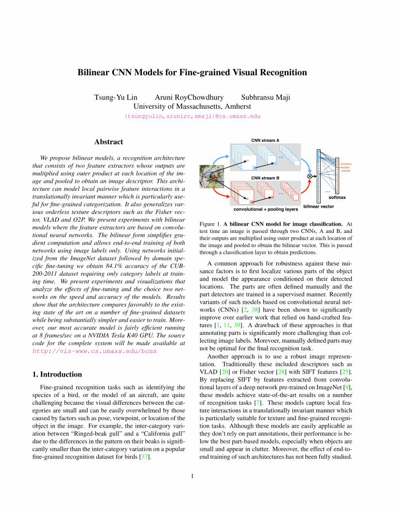
Figure 1. A bilinear CNN model for image classification. Attest time an image is passed through two CNNs, A and B, andtheir outputs are multiplied using outer product at each location ofthe image and pooled to obtain the bilinear vector. This is passedthrough a classification layer to obtain predictions.

A common approach for robustness against these nui-sance factors is to first localize various parts of the objectand model the appearance conditioned on their detectedlocations. The parts are often defined manually and thepart detectors are trained in a supervised manner. Recentlyvariants of such models based on convolutional neural net-works (CNNs) [2, 38] have been shown to significantlyimprove over earlier work that relied on hand-crafted fea-tures [1, 11, 39]. A drawback of these approaches is thatannotating parts is significantly more challenging than col-lecting image labels. Morevoer, manually defined parts maynot be optimal for the final recognition task.

Another approach is to use a robust image represen-tation. Traditionally these included descriptors such asVLAD [20] or Fisher vector [28] with SIFT features [25].By replacing SIFT by features extracted from convolu-tional layers of a deep network pre-trained on ImageNet [9],these models achieve state-of-the-art results on a numberof recognition tasks [7]. These models capture local fea-ture interactions in a translationally invariant manner whichis particularly suitable for texture and fine-grained recogni-tion tasks. Although these models are easily applicable asthey don’t rely on part annotations, their performance is be-low the best part-based models, especially when objects aresmall and appear in clutter. Moreover, the effect of end-to-end training of such architectures has not been fully studied.

1

Our main contribution is a recognition architecture thataddresses several drawbacks of both part-based and texturemodels (Fig. 1 and Sect. 2). It consists of two feature ex-tractors based on CNNs whose outputs are multiplied usingthe outer product at each location of the image and pooledacross locations to obtain an image descriptor. The outerproduct captures pairwise correlations between the featurechannels and can model part-feature interactions, e.g., if oneof the networks was a part detector and the other a localfeature extractor. The bilinear model also generalizes sev-eral widely used orderless texture descriptors such as theBag-of-Visual-Words [8], VLAD [20], Fisher vector [28],and second-order pooling (O2P) [3]. Moreover, the archi-tecture can be easily trained end-to-end unlike these texturedescriptions leading to significant improvements in perfor-mance. Although we don’t explore this connection further,our architecture is related to the two stream hypothesis ofvisual processing in the human brain [15] where there aretwo main pathways, or “streams”. The ventral stream (or,“what pathway”) is involved with object identification andrecognition. The dorsal stream (or, “where pathway”) is in-volved with processing the object’s spatial location relativeto the viewer. Since our model is linear in the outputs oftwo CNNs we call our approach bilinear CNNs.

Experiments are presented on fine-grained datasets ofbirds, aircrafts, and cars (Sect. 3). We initialize various bi-linear architectures using models trained on the ImageNet,in particular the “M-Net” of [5] and the “verydeep” network“D-Net” of [32]. Out of the box these networks do remark-ably well, e.g., features from the penultimate layer of thesenetworks achieve 52.7% and 61.0% accuracy on the CUB-200-2011 dataset [37] respectively. Fine-tuning improvesthe performance further to 58.8% and 70.4%. In compari-son a fine-tuned bilinear model consisting of a M-Net anda D-Net obtains 84.1% accuracy, outperforming a numberof existing methods that additionally rely on object or partannotations (e.g., 82.0% [21], or 75.7% [2]). We present ex-periments demonstrating the effect of fine-tuning on CNNbased Fisher vector models [7], the computational and ac-curacy tradeoffs of various bilinear CNN architectures, andways to break the symmetry in the bilinear models usinglow-dimensional projections. Finally, we present visualiza-tions of the models in Sect. 4 and conclude in Sect. 5.

1.1. Related work

Bilinear models were proposed by Tanenbaum and Free-man [33] to model two-factor variations, such as “style”and “content”, for images. While we also model two fac-tor variations arising out of part location and appearance,our goal is prediction. Our work is also related to bilinearclassifiers [29] that express the classifier as a product of twolow-rank matrices. However, in our model the features arebilinear, while the classifier itself is linear. Our reduced di-

mensionality models (Sect. 3.3) can be interpreted as bilin-ear classifiers. “Two-stream” architectures have been usedto analyze video where one networks models the temporalaspect, while the other models the spatial aspect [12, 31].Ours is a two-steam architecture for image classification.

A number of recent techniques have proposed to useCNN features in an orderless pooling setting such as Fishervector [7], or VLAD [14]. We compare against these meth-ods. Two other contemporaneous works are of interest.The first is the “hypercolumns” of [17] that jointly con-siders the activations from all the convolutional layers ofa CNN allowing finer grained resolution for localizationtasks. However, they do not consider pairwise interactionsbetween these features. The second is the “cross-layer pool-ing” method of [24] that considers pairwise interactions be-tween features of adjacent layers of a single CNN. Our bi-linear model can be seen as a generalization of this approachusing separate CNNs simplifying gradient computation fordomain specific fine-tuning.

2. Bilinear models for image classification

In this section we introduce a general formulation of abilinear model for image classification and then describe aspecific instantiation of the model using CNNs. We thenshow that various orderless pooling methods that are widelyused in computer vision can be written as bilinear models.

A bilinear model B for image classification consists of aquadruple B = (fA, fB , P, C). Here fA and fB are featurefunctions, P is a pooling function and C is a classificationfunction. A feature function is a mapping f : L ⇥ I !Rc⇥D that takes an image I and a location L and outputs afeature of size c⇥D. We refer to locations generally whichcan include position and scale. The feature outputs are com-bined at each location using the matrix outer product, i.e.,the bilinear feature combination of fA and fB at a locationl is given by bilinear(l, I, fA, fB) = fA(l, I)T fB(l, I).

Both fA and fB must have the feature dimension c tobe compatible. The reason for c > 1 will become clearlater when we show that various texture descriptors can bewritten as bilinear models. To obtain an image descrip-tor the pooling function P aggregates the bilinear featureacross all locations in the image. One choice of poolingis to simply sum all the bilinear features, i.e., �(I) =P

l2L bilinear(l, I, fA, fB). An alternative is max-pooling.Both these ignore the location of the features and are henceorderless. If fA and fB extract features of size C ⇥M andC ⇥ N respectively, then �(I) is of size M ⇥ N . The bi-linear vector obtained by reshaping �(I) to size MN ⇥ 1is a general purpose image descriptor that can be used witha classification function C. Intuitively, the bilinear form al-lows the outputs of the feature exactors fA and fB to beconditioned on each other by considering all their pairwiseinteractions similar to a quadratic kernel expansion.

2.1. Bilinear CNN models

A natural candidate for the feature function f is a CNNconsisting of a hierarchy of convolutional and pooling lay-ers. In our experiments we use CNNs pre-trained on theImageNet dataset [9] truncated at a convolutional layer in-cluding non-linearities as feature extractors. By pre-trainingwe benefit from additional training data when domain spe-cific data is scarce. This has been shown to be benefi-cial for a number of recognition tasks ranging from ob-ject detection, texture recognition, to fine-grained classifi-cation [6, 10, 13, 30]. Another advantage of using onlythe convolutional layers, is the resulting CNN can processimages of an arbitrary size in a single forward-propagationstep and produce outputs indexed by the location in the im-age and feature channel.

In all our experiments we use sum-pooling to aggregatethe bilinear features across the image. The resulting bilin-ear vector x = �(I) is then passed through signed square-root step (y sign(x)

p|x|), followed by `2 normaliza-

tion (z y/||y||2) inspired by [28]. This improves perfor-mance in practice (see supplementary material for experi-ments evaluating the effect of these normalizations). Forthe classification function C we use logistic regression orlinear SVM. This can be replaced with a multi-layer neuralnetwork if non-linearity is desirable.

End-to-end training Since the overall architectureis a directed acyclic graph the parameters can be trainedby back-propagating the gradients of the classification loss(e.g., conditional log-likelihood). The bilinear form simpli-fies the gradients at the pooling layer. If the outputs of thetwo networks are matrices A and B of size L⇥M and L⇥Nrespectively, then the pooled bilinear feature is x = AT B ofsize M ⇥N . Let d`/dx be the gradient of the loss function` wrto. x, then by chain rule of gradients we have:

d`

dA= B

✓d`

dx

◆T

,d`

dB= A

✓d`

dx

◆. (1)

The gradient of the classification and normalization layeris straightforward, and the gradient of the layers below thepooling layer can be computed using the chain rule. Thescheme is illustrated in Fig 2. We fine-tune our model usingstochastic gradient descent with mini-batches with weightdecay and momentum as described in Sect 3.1.

2.2. Relation to orderless texture descriptors

In this section we show that various orderless texture de-scriptors can be written as bilinear models. These methodstypically extract local features such as SIFT densely froman image and pass them through a non-linear encoder ⌘.A popular encoder is a Gaussian mixture model (GMM)that assigns features to the k centers, C = [µ1, µ2, . . . , µk],

`2sqrt

d`

dB � A

✓d`

dz

dz

dy

dy

dx

◆

d`

dA � B

✓d`

dz

dz

dy

dy

dx

◆T

A

B

x = AT B y z

Figure 2. Computing gradients in the bilinear CNN model.

based on their GMM posterior. When these encoded de-scriptors are sum-pooled across the image we obtain theBag-of-Visual-Words (BoVW) model [8]. Using the bilin-ear notation this can be written as B = (⌘(fsift), 1, P, C),i.e., a bilinear model where the second feature extractor fB

simply returns 1 for all input.The Vector of Locally Aggregated Descriptors (VLAD)

descriptor [20] aggregates the first order statistics of theSIFT descriptors. Each descriptor x is encoded as (x �µk) ⌦ ⌘(x), where ⌦ is the kroneker product and µk isthe closest center to x. In the VLAD model ⌘(x) is setto one for the closest center and zero elsewhere, also re-ferred to as “hard assignment.” These are aggregated acrossthe image by sum pooling. Thus VLAD can be written asa bilinear model with fA = [x � µ1;x � µ2; . . . ;x � µk],i.e., fA has k rows each corresponding to each center, andfB = diag(⌘(x)), a matrix with ⌘(x) in the diagonal andzero elsewhere. Notice that the feature extractors for VLADoutput a matrix with k > 1 rows.

The Fisher vector (FV) [28] computes both the first order↵i = ⌃

� 12

i (x� µi) and second order �i = ⌃�1i (x� µi)�

(x � µi) � 1 statistics, which are aggregated weighted by⌘(x). Here µi and ⌃i is the mean and covariance of the ith

GMM component respectively and� denotes element-wisemultiplication. This can be written as a bilinear model withfA = [↵1 �1; ↵2 �2; . . . ; ↵k �k] and fB = diag(⌘(x)).

In both VLAD and FV the encoding function ⌘ can beviewed as a part detector. Indeed it has been experimen-tally observed that the GMM centers tend to localize faciallandmarks when trained on faces [27]. Thus, these mod-els simultaneously localize parts and describe their appear-ance using joint statistics of the encoding ⌘(x) and featurex which might explain their effectiveness on fine-grainedrecognition tasks. Another successful method for semanticsegmentation is the second-order pooling (O2P) method [3]that pools the covariance of SIFT features extracted locallyfollowed by non-linearities. This is simply the bilinearmodel B = (fsift, fsift, P, C).

In all these descriptors both fA and fB are based on thesame underlying feature x, e.g., SIFT or CNN. One maywant to use different features to detect parts and to describetheir appearance. Furthermore, these methods typically donot learn the feature extractor functions and only the pa-rameters of the encoder ⌘ and the classifier function C arelearned on a new dataset. Even when CNN features are

pooled using FV method, training is usually not done end-to-end since it is cumbersome to compute the gradients ofthe network since fA and fB both depend on the x. Ourmain insight is to decouple fA and fB which makes thegradient computation significantly easier (Eqn. 1), allowingus to fine-tune the feature extractors on specific domains.As our experiments show this significantly improves the ac-curacy. For Fisher vector CNN models we show that evenwhen fine-tuning is done indirectly, i.e., using a differentpooling method, the overall performance improves.

3. Experiments

3.1. Methods

In addition to SIFT, we consider two CNNs for ex-tracting features in the bilinear models – the M-Net of [5]and the verydeep network D-Net of [32] consisting of 16convolutional and pooling layers. The D-Net is more ac-curate but is about 7⇥ slower on a Tesla K40 GPU. Inboth cases we consider the outputs of the last convolutionallayer with non-linearities as feature extractors, i.e., layer 14(conv5+relu) for the M-net and layer 30 (conv5 4+relu) forthe D-Net. Remarkably, this represents less than 10% ofthe total number of parameters in the CNNs. Both thesenetworks produce 1⇥512 dimensional features at each lo-cation. In addition to previous work, we evaluate the fol-lowing methods keeping the training and evaluation setupidentical for a detailed comparison.

I. CNN with fully-connected layers (FC-CNN) This isbased on the features extracted from the last fully-connectedlayer before the softmax layer of the CNN. The input im-age is resized to 224⇥224 (the input size of the CNN)and mean-subtracted before propagating it though the CNN.For fine-tuning we replace the 1000-way classification layertrained on ImageNet dataset with a k-way softmax layerwhere k is the number of classes in the fine-grained dataset.The parameters of the softmax layer are initialized ran-domly and we continue training the network on the datasetfor several epochs at a smaller learning rate while monitor-ing the validation error. Once the networks are trained, thelayer before the softmax layer is used to extract features.

II. Fisher vector with CNN features (FV-CNN) Thisdenotes the method of [7] that builds a descriptor using FVpooling of CNN filter bank responses with 64 GMM com-ponents. One modification is that we first resize the im-age to 448⇥448 pixels, i.e., twice the resolution the CNNswere trained on and pool features from a single-scale. Thisleads to a slight reduction in performance, but we choose thesingle-scale setting because (i) multi-scale is likely to im-prove results for all methods, and (ii) this keeps the feature

extraction in FV-CNN and B-CNN identical making com-parisons easier. Fine-tuned FV-CNN results are reported us-ing the fine-tuned FC-CNN models since direct fine-tuningis non-trivial. Surprisingly we found that this indirect train-ing improves accuracy outperforming the non fine-tuned butmulti-scale results (Sect 3.2.1) .

III. Fisher vector with SIFT (FV-SIFT) We imple-mented a FV baseline using dense SIFT features [28] ex-tracted using VLFEAT [35]. Keeping the settings identicalto FV-CNN, the input image is first resized to 448⇥448 be-fore SIFT features with binsize of 8 pixels are computeddensely across the image with a stride of 4 pixels. The fea-tures are PCA projected to 80 dimensions before learning aGMM with 256 components.

IV. Bilinear CNN model (B-CNN) We consider sev-eral bilinear CNN models – (i) initialized with two M-netsdenoted by B-CNN [M,M], (ii) initialized with a D-Net andan M-Net denoted by B-CNN [D,M], and (iii) initializedwith two D-nets denoted by B-CNN [D,D]. Identical to thesetting in FV-CNN, the input images are first resized to448⇥448 and features are extracted using the two networksbefore bilinear combination, sum-pooling, and normaliza-tion. The D-Net produces a slightly larger output 28⇥28compared to 27⇥27 of the M-Net. We simply downsam-ple the output of the D-Net by ignoring a row and column.The pooled bilinear feature is of size 512⇥512, which com-parable to that of FV-CNN (512⇥128) and FV-SIFT (80 ⇥512). For fine-tuning we add a k-way softmax layer. Weadopt the two step training procedure of [2] where we firsttrain the last layer using logistic regression, a convex opti-mization problem, followed by fine-tuning the entire modelusing back-propagation for several epochs (about 45 – 100depending on the dataset and model) at a relatively smalllearning rate (⌘ = 0.001). Across the datasets we found thehyperparameters for fine-tuning were fairly consistent.

Classifier training In all our experiments once fine-tuning is done, training and validation sets are combinedand one-vs-all linear SVMs on the extracted features aretrained by setting the learning hyperparameter Csvm = 1.Since our features are `2 normalized the optimal of Csvm islikely to be independent of the dataset. The trained classi-fiers are calibrated by scaling the weight vector such thatthe median scores of positive and negative training exam-ples are at +1 and �1 respectively. For each dataset wedouble the training data by flipping images and and at testtime we average the predictions of the image and its flippedcopy and assign the class with the highest score. Directlyusing the softmax predictions results in a slight drop in ac-curacy compared to linear SVMs. Performance is measuredas the fraction of correct image predictions for all datasets.

3.2. Datasets and results

We report results on three fine-grained recognitiondatasets – birds [37], aircrafts [26], and cars [22]. Birds aresmaller in the image compared to aircrafts stressing the roleof part localization. Cars and birds also appear in more clut-ter compared to aircrafts. Fig. 3 shows some examples fromthese datasets. Approximate feature extraction speeds ofour MatConvNet [36] based implementation and per-imageaccuracies for various methods are shown in Tab. 1.

3.2.1 Bird species classification

The CUB-200-2011 [37] dataset contains 11,788 images of200 bird species. We evaluate our methods in two protocols– “birds” where the object bounding-box is not providedboth at training and test time, and “birds + box” where thebounding-box is provided both at training and test time. Forthis dataset we crop a central square patch and resize it to448⇥448 instead of resizing the image, which performedslightly better.

Several methods report results requiring varying degreesof supervision such as part annotation or bounding-boxesat training and test time. We refer readers to [2] that has acomprehensive discussion of results on this dataset. A moreup-to-date set of results can be found in [21] who recentlyreported excellent performance using on this dataset lever-aging more accurate CNN models with a method to trainpart detectors in a weakly supervised manner.

Comparison to baselines Without object bounding-boxes the fine-tuned FC-CNN [M] and FC-CNN [D]achieve accuracy of 58.8% and 70.4% respectively. Evenwithout fine-tuning the FV models achieve better resultsthan the corresponding fine-tuned FC models – FV-CNN[M] 61.1%, and FV-CNN [D] 71.3%. We evaluated FVmodels with the fine-tuned FC models and surprisinglyfound that this improves performance, e.g., FV-CNN [D]improves to 74.7%. This shows that domain specific fine-tuning can be useful even when early convolutional layersof a CNN are used as features. Moreover, if FV-CNN fine-tuning was done to directly optimize its performance, re-sults may further improve. However, as we discussed earliersuch direct training is hard due to the difficultly in comput-ing the gradients. We also note that the FV-CNN resultswith indirect fine-tuning outperforms the multi-scale resultsreported in [7] – 49.9% using M-Net and 66.7% using D-Net. The bilinear CNN models are substantially more ac-curate than the corresponding FC and FV models. Withoutfine-tuning B-CNN [M,M] achieves 72.0%, B-CNN [D,M]achieves 80.1%, while B-CNN [D,D] achieves 80.1% accu-racy, even outperforming the fine-tuned FC and FV mod-els. Fine-tuning improves performance of these models byabout 4-6% to 78.1%, 84.1% and 84.0% respectively.

Figure 3. Examples from (left) birds dataset [37], (center) aircraftdataset [26], and (right) cars dataset [22] used in our experiments.

The trends when bounding-boxes are used at trainingand test times are similar. All the methods benefit fromthe added supervision. The performance of the FC and FVmodels improves significantly – roughly 10% for the FCand FV models with the M-Net and 6% for those with theD-Net. However, the most accurate B-CNN model benefitsless than 1% suggesting a greater invariance to the locationof parts in the image.

Comparison to previous work Two methods thatperform well on this dataset when bounding-boxes arenot available at test time are 73.9% of the “part-based R-CNN” [38] and 75.7% of the “pose-normalized CNN” [2].Although the notion of parts differ, both these methods arebased on a two step process of part detection followed byCNN based classifier. They also rely on part annotationduring training. Our method outperforms these methods bya significant margin without relying on part or bounding-box annotations. Moreover, it is significantly simpler andfaster – the bilinear feature computation using B-CNN[M,M] runs at 87 frames/sec, while B-CNN [D,M] runs at8 frames/sec. Compared to the part detection step whichrequires thousands of network evaluations on region pro-posals [13] our method effectively requires only two evalu-ations and hence is significantly faster. We note that the ac-curacy of these methods can be improved by replacing theunderlying AlexNet CNN [23] with the more accurate butsignificantly slower D-Net. Recently [21] reported 82.0%accuracy using a weakly supervised method to learn partdetectors followed by the part-based analysis of [38] usinga D-Net. However, this method relies on object bounding-boxes for training. Another recent approach called the “spa-tial transformer networks” reports 84.1% accuracy [19] us-ing the Inception CNN architecture with batch normaliza-tion [18]. This approach also does not require object or partbounding-boxes at training time.

When bounding-boxes are used at test time all meth-ods improve. The results of [38] improves to 76.4%. An-other recently proposed method that reports strong resultson this setting is the “cross-layer pooling” method of [24]that considers pairwise features extracted from two differentlayers of a CNN. Using AlexNet they report an accuracyof 73.5%. Our B-CNN model with two M-Nets methodachieves 80.4% outperforming this by a significant margin.

birds birds + box aircrafts cars

method w/o ft w/ ft w/o ft w/ ft w/o ft w/ ft w/o ft w/ ft FPS

FV-SIFT 18.8 - 22.4 - 61.0 - 59.2 - 10†

FC-CNN [M] 52.7 58.8 58.0 65.7 44.4 57.3 37.3 58.6 124FC-CNN [D] 61.0 70.4 65.3 76.4 45.0 74.1 36.5 79.8 43FV-CNN [M] 61.1 64.1 67.2 69.6 64.3 70.1 70.8 77.2 23FV-CNN [D] 71.3 74.7 74.4 77.5 70.4 77.6 75.2 85.7 8B-CNN [M,M] 72.0 78.1 74.2 80.4 72.7 77.9 77.8 86.5 87B-CNN [D,M] 80.1 84.1 81.3 85.1 78.4 83.9 83.9 91.3 8B-CNN [D,D] 80.1 84.0 80.1 84.8 76.8 84.1 82.9 90.6 10Previous work 84.1 [19], 82.0 [21] 82.8 [21], 73.5 [24] 72.5 [4], 80.7 [16] 92.6 [21], 82.7 [16] †on a cpu

73.9 [38], 75.7 [2] 73.0 [7], 76.4 [38] 78.0 [4]

Table 1. Classification results. We report per-image accuracy on the CUB-200-2011 dataset [37] without (birds) and with bounding-boxes(birds + box), aircrafts dataset [26] and cars dataset [22]. FV-SIFT is the Fisher vector representation with SIFT features, FC-CNN usesfeatures from the last fully connected layer of a CNN, and FV-CNN uses FV pooling of CNN filter banks [7]. B-CNN is the bilinearmodel consisting of two CNNs shown in brackets. For each model results are shown without and with domain specific fine-tuning. ForFV-CNN fine-tuned results are reported using FC-CNN fine-tuned models. We report results using the M-Net [5] and D-Net [32] forvarious approaches. The feature extraction speeds (frames/sec) on a Tesla K40 GPU for various methods using our MatConvNet/VLFEATbased implementation are shown on the rightmost column. See Sect. 3 for details of the methods and a discussion of results.

Common mistakes Fig. 4 shows the top six pairs ofclasses that are confused by our fine-tuned B-CNN [D,M]model. The most confused pair of classes is “Americancrow” and “Common raven”, which look remarkably simi-lar. A quick search on the web reveals that the differenceslie in the wing-spans, habitat, and voice, none of which areeasy to measure from the image. Other commonly confusedclasses are also visually similar – various Shrikes, Terns,Flycatchers, Cormorants, etc. We note that the dataset hasan estimated 4.4% label noise hence some of these errorsmay be incorrect [34].

American Crow Common Raven

Loggerhead Shrike Great Grey Shrike

Caspian Tern Elegant Tern

Acadian Flycatcher Yellow bellied Flycatcher

Brandt Cormorant Pelagic Cormorant

Glaucous winged Gull Western Gull

Figure 4. Top six pairs of classes that are most confused witheach other. In each row we show the images in the test set thatwere most confidently classified as the class in the other column.

3.2.2 Aircraft variant classification

The FGVC-aircraft dataset [26] consists of 10,000 imagesof 100 aircraft variants, and was introduced as a part ofthe FGComp 2013 challenge. The task involves discrim-inating variants such as the Boeing 737-300 from Boeing737-400. The differences are subtle, e.g., one may be ableto distinguish them by counting the number of windows inthe model. Unlike birds, airplanes tend to occupy a signif-icantly larger portion of the image and appear in relativelyclear background. Airplanes also have a smaller represen-tation in the ImageNet dataset compared to birds.

Comparison to baselines The trends among the base-lines are similar to those in birds with a few exceptions. TheFV-SIFT baseline is remarkably good (61.0%) outperform-ing some of the fine-tuned FC-CNN baselines. Comparedto the birds, the effect of fine-tuning FC-CNN [D] is sig-nificantly larger (45.0%! 74.1%) perhaps due to a largerdomain shift from the ImageNet dataset. The fine-tuned FV-CNN models are also significantly better than the FC-CNNmodels in this dataset. Once again indirect fine-tuning ofthe FV-CNN models via fine-tuning FC-CNN helps by 5-7%. The best performance of 84.1% is achieved by the B-CNN [D,D] model. Fine-tuning leads to 7% improvementin its accuracy.

Comparison to previous work This dataset does notcome with part annotations hence several top performingmethods for the birds dataset are not applicable here. Wealso compare against the results for “track 2”, i.e., w/obounding-boxes, at the FGComp 2013 challenge website 1.

1https://sites.google.com/site/fgcomp2013/results

The best performing method [16] is a heavily engineeredFV-SIFT which achieves 80.7% accuracy. Notable differ-ences between our baseline FV-SIFT and theirs are (i) largerdictionary (256! 1024), (ii) Spatial pyramid pooling (1⇥1! 1⇥1 + 3⇥1), (iii) multiple SIFT variants, and (iv) multi-scale SIFT. The next best method is the “symbiotic seg-mentation” approach of [4] that achieves 72.5% accuracy.However, this method requires bounding-box annotations attraining time to learn a detector which is refined to a fore-ground mask. The B-CNN models outperform these meth-ods by a significant margin. The results on this dataset showthat orderless pooling methods are still of considerable im-portance – they can be easily applied to new datasets as theyonly need image labels for training.

3.2.3 Car model classification

The cars dataset [22] contains 16,185 images of 196 classes.Categories are typically at the level of Make, Model, Year,e.g., “2012 Tesla Model S” or ‘2012 BMW M3 coupe.”Compared to aircrafts, cars are smaller and appear in amore cluttered background. Thus object and part localiza-tion may play a more significant role here. This dataset wasalso part of the FGComp 2013 challenge.

Comparison to baselines FV-SIFT once again doeswell on this dataset achieving 59.2% accuracy. Fine-tuningsignificantly improves performance of the FC-CNN models,e.g., 36.5%! 79.8% for FC-CNN [D], suggesting that thedomain shift is larger here. The fine-tuned FV-CNN mod-els do significantly better, especially with the D-Net whichobtains 85.7% accuracy. Once again the bilinear CNN mod-els outperform all the other baselines with the B-CNN [D,M] model achieving 91.3% accuracy. Fine-tuning improvesresults by 7-8% for the B-CNN models.

Comparison to previous work The best accuracyon this dataset is 92.6% obtained by the recently proposedmethod [21]. We also compare against the winning meth-ods from the FGComp 2013 challenge. The SIFT ensem-ble [16] won this category (during the challenge) achievinga remarkable 82.7% accuracy. The symbiotic segmentationachieved 78.0% accuracy. The fine-tuned B-CNN [D,M]obtains 91.3% significantly outperforming the SIFT ensem-ble, and nearly matching [21] which requires bounding-boxes during training. The results when bounding-boxesare available at test time can be seen in “track 1” of theFGComp 2013 challenge and are also summarized in [16].The SIFT ensemble improves significantly with the additionof bounding-boxes (82.7% ! 87.9%) in the cars datasetcompared to aircraft dataset where it improves marginally(80.7%! 81.5%). This shows that localization in the carsdataset is more important than in aircrafts. Our bilinear

models have a clear advantage over FV models in this set-ting since it can learn to ignore the background clutter.

3.3. Low dimensional bilinear CNN models

The bilinear CNN models that are symmetrically initial-ized will remain symmetric after fine-tuning since the gra-dients for the two networks are identical. Although thisis good for efficiency since the model can be implementedwith just a single CNN evaluation, this may be suboptimalsince the model doesn’t explore the space of solutions thatcan arise from different CNNs. We experimented with sev-eral ways to break the symmetry between the two featureextractors. The first is “dropout” [23] where during train-ing a random subset of outputs in each layer are set to zerowhich will cause gradients of the CNN to differ. However,we found that this led to 1% loss in performance on birds.We also experimented with a structured variant of dropoutwhere we randomly zero out the rows and columns of thethe pooled bilinear feature (AT B). Unfortunately, this alsoperformed 1% worse. We hypothesize that the model isstuck at a local minima as there isn’t enough training dataduring fine-tuning. On larger datasets such schemes may bemore important.

Our second idea is to project one of the CNN outputsto a lower dimension breaking the symmetry. This can beimplemented by adding another layer of the CNN with aconvolutional filter of size 1⇥1⇥N⇥D where N is the num-ber of channels in the output of the CNN and D is the pro-jected dimension. We initialize the parameters using PCA,projecting the 512 dimensional output of the M-Net to 64.Centering is absorbed into a bias term for each projection.

This projection also reduces the number of parametersin the model. For the B-CNN [M,M] model with k classesthere are 512⇥512⇥k parameters in the classification layer.With the projection there are only 512⇥64⇥k parameters inthe classification layer, plus 512⇥64 parameters in the pro-jection layer. Thus, the resulting classification function Ccan also be viewed as a “bilinear classifier” [29] – a productof two low-rank matrices.

However, PCA projection alone worsens performance.Fig. 5 shows the average precision-recall curves across the200 classes for various models. On birds the mean averageprecision (mAP) of the non fine-tuned model w/o PCA is72.5% which drops to 72.0% w/ PCA. Since the projectionis just another layer in the CNN, it can be jointly trainedwith the rest of the parameters in the bilinear model. Thisimproves mAP to 80.1% even outperforming the originalfine-tuned model that achieves 79.8%. Moreover the pro-jected model is also slightly faster. Finally, we note thatwhen PCA was applied to both the networks the resultswere significantly worse even with fine-tuning suggestingthat sparse outputs are preferable when pooling.

0 0.1 0.2 0.3 0.4 0.5 0.6 0.7 0.8 0.9 10

0.1

0.2

0.3

0.4

0.5

0.6

0.7

0.8

0.9

1

recall

pre

cisi

on

72.5 (m,m)79.8 (m,m)+ft

72.0 (m,m64

pca)

80.1 (m,m64

pca)+ft

Figure 5. Low dimensional B-CNN (M,M) models.

4. Discussion

One of the motivations for the bilinear model was themodular separation of factors that affect the overall appear-ance. But do the networks specialize into roles of local-ization (“where”) and appearance modeling (“what”) wheninitialized asymmetrically and fine-tuned? Fig. 6 shows thetop activations of several filters in the D-Net and M-Net ofthe fine-tuned B-CNN [D, M] model. These visualizationssuggest that the roles of the two networks are not clearlyseparated. Both these networks tend to activate strongly onhighly specific semantic parts. For example, the last rowof D-Net detects “tufted heads”, which can be seen as ei-ther part or a feature (visualizations on other datasets canbe found in the supplementary material).

The above visualizations also suggests that the role offeatures and parts in fine-grained recognition tasks can betraded. For instance, consider the task of gender recogni-tion. One approach is to first train a gender-neutral face de-tector and followed by a gender classifier. However, it maybe better to train a gender-specific face detector instead. Byjointly training fA and fB the bilinear model can effectivelytrade-off the representation power of the features based onthe data. Thus, manually defined parts not only requires sig-nificant annotation effort but also is likely to be sub-optimalwhen enough training data is available.

Our bilinear CNN models had two feature extractorswhose processing pathways separated early, but some ofthe early processing in the CNNs may be shared. Thus onecan design a more efficient architecture where the featureextractors share the first few stages of their processing andthen bifurcate to specialize in their own tasks. As long as thestructure of the network is a directed acyclic graph standardback-propagation training applies. Our architecture is alsomodular. For example, one could append additional featurechannels, either hand-crafted or CNNs, to the either fA orfB only update the trainable parameters during fine-tuning.Thus, one could train models with desired semantics, e.g.,color, describable textures [6], or parts, for predicting at-

D-Net M-Net

Figure 6. Patches with the highest activations for several filters ofthe fine-tuned B-CNN (D, M) model on CUB-200-2011 dataset.

tributes or sentences. Finally, one could extend the bilinearmodel to a trilinear model to factor out another source ofvariation. This could be applied for action recognition overtime where a third network could look at optical flow.

5. Conclusion

We presented bilinear CNN models and demonstratedtheir effectiveness on various fine-grained recognitiondatasets. Remarkably, the performance is comparable tomethods that use the similar CNNs and additionally relyon part or bounding-box annotations for training. Our hy-pothesis is that our intuition of features that can be extractedfrom CNNs are poor and manually defined parts can be sub-optimal in a pipelined architecture. The proposed modelscan be fine-tuned end-to-end using image labels which re-sults in significant improvements over other orderless tex-ture descriptors based on CNNs such as the FV-CNN.

The model is also efficient requiring only two CNN eval-uations on a 448⇥448 image. Our MatConvNet [36] basedimplementation of the asymmetric B-CNN [D,M] runs at8 frames/sec on a Tesla K40 GPU for the feature extrac-tion step, only a small constant factor slower than a sin-gle D-Net and significantly faster than methods that relyon object or part detections. The symmetric models arefaster since they can be implemented with just a singleCNN evaluation, e.g., B-CNN [M,M] runs at 87 frames/sec,while the B-CNN [D,D] runs at 10 frames/sec. The sourcecode for the complete system will be made available athttp://vis-www.cs.umass.edu/bcnn

Acknowledgement This research was supported in part bythe Office of the Director of National Intelligence (ODNI),Intelligence Advanced Research Projects Activity (IARPA)under contract number 2014-14071600010. The GPUs usedin this research were generously donated by NVIDIA.

References

[1] L. Bourdev, S. Maji, and J. Malik. Describing people: Aposelet-based approach to attribute classification. In ICCV,2011. 1

[2] S. Branson, G. V. Horn, S. Belongie, and P. Perona. Birdspecies categorization using pose normalized deep convolu-tional nets. In BMVC, 2014. 1, 2, 4, 5, 6

[3] J. Carreira, R. Caseiro, J. Batista, and C. Sminchisescu. Se-mantic segmentation with second-order pooling. In ECCV.2012. 2, 3

[4] Y. Chai, V. Lempitsky, and A. Zisserman. Symbiotic seg-mentation and part localization for fine-grained categoriza-tion. In ICCV, 2013. 6, 7

[5] K. Chatfield, K. Simonyan, A. Vedaldi, and A. Zisserman.Return of the devil in the details: Delving deep into convo-lutional nets. In BMVC, 2014. 2, 4, 6

[6] M. Cimpoi, S. Maji, I. Kokkinos, S. Mohamed, andA. Vedaldi. Describing textures in the wild. In CVPR, 2014.3, 8

[7] M. Cimpoi, S. Maji, and A. Vedaldi. Deep filter banks fortexture recognition and description. In CVPR, 2015. 1, 2, 4,5, 6

[8] G. Csurka, C. R. Dance, L. Dan, J. Willamowski, andC. Bray. Visual categorization with bags of keypoints. InECCV Workshop on Stat. Learn. in Comp. Vision, 2004. 2, 3

[9] J. Deng, W. Dong, R. Socher, L.-J. Li, K. Li, and L. Fei-Fei.ImageNet: A Large-Scale Hierarchical Image Database. InCVPR, 2009. 1, 3

[10] J. Donahue, Y. Jia, O. Vinyals, J. Hoffman, N. Zhang,E. Tzeng, and T. Darrell. Decaf: A deep convolutional acti-vation feature for generic visual recognition. In ICML, 2013.3

[11] R. Farrell, O. Oza, N. Zhang, V. I. Morariu, T. Darrell, andL. S. Davis. Birdlets: Subordinate categorization using volu-metric primitives and pose-normalized appearance. In ICCV,2011. 1

[12] K. Fragkiadaki, P. Arbelaez, P. Felsen, and J. Malik. Learn-ing to segment moving objects in videos. In CVPR, 2015.2

[13] R. B. Girshick, J. Donahue, T. Darrell, and J. Malik. Richfeature hierarchies for accurate object detection and semanticsegmentation. In CVPR, 2014. 3, 5

[14] Y. Gong, L. Wang, R. Guo, and S. Lazebnik. Multi-scaleorderless pooling of deep convolutional activation features.In ECCV, 2014. 2

[15] M. A. Goodale and A. D. Milner. Separate visual path-ways for perception and action. Trends in neurosciences,15(1):20–25, 1992. 2

[16] P.-H. Gosselin, N. Murray, H. Jegou, and F. Perronnin. Re-visiting the fisher vector for fine-grained classification. Pat-tern Recognition Letters, 49:92–98, 2014. 6, 7

[17] B. Hariharan, P. Arbelaez, R. Girshick, and J. Malik. Hyper-columns for object segmentation and fine-grained localiza-tion. In CVPR, 2015. 2

[18] S. Ioffe and C. Szegedy. Batch normalization: Acceleratingdeep network training by reducing internal covariate shift. InICML, 2015. 5

[19] M. Jaderberg, K. Simonyan, A. Zisserman, andK. Kavukcuoglu. Spatial transformer networks. CoRR,

abs/1506.02025, 2015. 5, 6[20] H. Jegou, M. Douze, C. Schmid, and P. Perez. Aggregating

local descriptors into a compact image representation. InCVPR, 2010. 1, 2, 3

[21] J. Krause, H. Jin, J. Yang, and L. Fei-Fei. Fine-grainedrecognition without part annotations. In CVPR, 2015. 2,5, 6, 7

[22] J. Krause, M. Stark, J. Deng, and L. Fei-Fei. 3d object repre-sentations for fine-grained categorization. In 3D Represen-tation and Recognition Workshop, at ICCV, 2013. 5, 6, 7

[23] A. Krizhevsky, I. Sutskever, and G. E. Hinton. Imagenetclassification with deep convolutional neural networks. InNIPS, 2012. 5, 7

[24] L. Liu, C. Shen, and A. van den Hengel. The treasure beneathconvolutional layers: Cross-convolutional-layer pooling forimage classification. In CVPR, 2015. 2, 5, 6

[25] D. G. Lowe. Object recognition from local scale-invariantfeatures. In ICCV, 1999. 1

[26] S. Maji, E. Rahtu, J. Kannala, M. Blaschko, and A. Vedaldi.Fine-grained visual classification of aircraft. arXiv preprintarXiv:1306.5151, 2013. 5, 6

[27] O. M. Parkhi, K. Simonyan, A. Vedaldi, and A. Zisserman. Acompact and discriminative face track descriptor. In CVPR,2014. 3

[28] F. Perronnin, J. Sanchez, and T. Mensink. Improving theFisher kernel for large-scale image classification. In ECCV,2010. 1, 2, 3, 4

[29] H. Pirsiavash, D. Ramanan, and C. C. Fowlkes. Bilinear clas-sifiers for visual recognition. In NIPS. 2009. 2, 7

[30] A. S. Razavin, H. Azizpour, J. Sullivan, and S. Carlsson. Cnnfeatures off-the-shelf: An astounding baseline for recogni-tion. In DeepVision workshop, 2014. 3

[31] K. Simonyan and A. Zisserman. Two-stream convolutionalnetworks for action recognition in videos. In NIPS, 2014. 2

[32] K. Simonyan and A. Zisserman. Very deep convolutionalnetworks for large-scale image recognition. In ICLR, 2015.2, 4, 6

[33] J. B. Tenenbaum and W. T. Freeman. Separating styleand content with bilinear models. Neural computation,12(6):1247–1283, 2000. 2

[34] G. Van Horn, S. Branson, R. Farrell, S. Haber, J. Barry,P. Ipeirotis, P. Perona, and S. Belongie. Building a birdrecognition app and large scale dataset with citizen scientists:The fine print in fine-grained dataset collection. In CVPR,2015. 6

[35] A. Vedaldi and B. Fulkerson. VLFeat: An open and portablelibrary of computer vision algorithms. http://www.

vlfeat.org/, 2008. 4[36] A. Vedaldi and K. Lenc. MatConvNet – Convolutional Neu-

ral Networks for MATLAB. In ACMMM, 2015. 5, 8[37] C. Wah, S. Branson, P. Welinder, P. Perona, and S. Belongie.

The Caltech-UCSD Birds-200-2011 Dataset. Technical Re-port CNS-TR-2011-001, CalTech, 2011. 1, 2, 5, 6

[38] N. Zhang, J. Donahue, R. Girshickr, and T. Darrell. Part-based R-CNNs for fine-grained category detection. InECCV, 2014. 1, 5, 6

[39] N. Zhang, R. Farrell, and T. Darrell. Pose pooling kernels forsub-category recognition. In CVPR, 2012. 1