bilinear spatiotemporal basis models - computer...

17

Bilinear Spatiotemporal Basis Models

IJAZ AKHTERLUMS School of Science and Engineering and Disney Research PittsburghTOMAS SIMONCarnegie Mellon University and Disney Research PittsburghSOHAIB KHANLUMS School of Science and EngineeringIAIN MATTHEWSDisney Research Pittsburgh and Carnegie Mellon UniversityandYASER SHEIKHCarnegie Mellon University

A variety of dynamic objects, such as faces, bodies, and cloth, are repre-sented in computer graphics as a collection of moving spatial landmarks.Spatiotemporal data is inherent in a number of graphics applications includ-ing animation, simulation, and object and camera tracking. The principalmodes of variation in the spatial geometry of objects are typically modeledusing dimensionality reduction techniques, while concurrently, trajectoryrepresentations like splines and autoregressive models are widely used toexploit the temporal regularity of deformation. In this article, we present thebilinear spatiotemporal basis as a model that simultaneously exploits spatialand temporal regularity while maintaining the ability to generalize well tonew sequences. This factorization allows the use of analytical, predefinedfunctions to represent temporal variation (e.g., B-Splines or the Discrete Co-sine Transform) resulting in efficient model representation and estimation.The model can be interpreted as representing the data as a linear combina-tion of spatiotemporal sequences consisting of shape modes oscillating overtime at key frequencies. We apply the bilinear model to natural spatiotem-poral phenomena, including face, body, and cloth motion data, and compare

I. Akhter and T. Simon contributed equally to this work.Authors’ addresses: I. Akhter, LUMS School of Science and Engineering,Disney Research Pittsburgh, Pittsburgh, PA; email: [email protected];T. Simon, Carnegie Mellon University, Disney Research Pittsburgh,Pittsburgh, PA; email: [email protected]; S. Khan, LUMS School ofScience and Engineering, Lahore University of Management Sciences,Lahore, Pakistan; email: [email protected]; I. Mathews, Disney Re-search Pittsburgh, Pittsburgh, PA, Carnegie Mellon University; email:[email protected]; Y. Sheikh, Department of Computer Science,Carnegie Mellon University; email: [email protected] to make digital or hard copies of part or all of this work forpersonal or classroom use is granted without fee provided that copies arenot made or distributed for profit or commercial advantage and that copiesshow this notice on the first page or initial screen of a display along withthe full citation. Copyrights for components of this work owned by othersthan ACM must be honored. Abstracting with credit is permitted. To copyotherwise, to republish, to post on servers, to redistribute to lists, or to useany component of this work in other works requires prior specific permissionand/or a fee. Permissions may be requested from Publications Dept., ACM,Inc., 2 Penn Plaza, Suite 701, New York, NY 10121-0701 USA, fax +1(212) 869-0481, or [email protected]© 2012 ACM 0730-0301/2012/04-ART17 $10.00

DOI 10.1145/2159516.2159523http://doi.acm.org/10.1145/2159516.2159523

it in terms of compaction, generalization ability, predictive precision, andefficiency to existing models. We demonstrate the application of the modelto a number of graphics tasks including labeling, gap-filling, denoising, andmotion touch-up.

Categories and Subject Descriptors: I.3.7 [Computer Graphics]:Three-Dimensional Graphics and Realism—Animation; I.3.5 [ComputerGraphics]: Computational Geometry and Object Modeling—Physicallybased modeling

General Terms: Algorithms, Theory, Measurement

Additional Key Words and Phrases: Bilinear models, spatiotemporal, motiondata, motion capture

ACM Reference Format:

Akhter, I., Simon, T., Khan, S., Matthews, I., and Sheikh, Y. 2012. Bilinearspatiotemporal basis models. ACM Trans. Graph. 31, 2, Article 17 (April2012), 12 pages.DOI = 10.1145/2159516.2159523http://doi.acm.org/10.1145/2159516.2159523

1. INTRODUCTION

We present a compact and generalizable model of time-varying spa-tial data that can simultaneously capture the spatial and the temporalcorrelations inherent in the data while remaining efficient in its re-quirements of training data and memory. Time-varying spatial datais widely used to represent animated characters in computer games,marker data in motion capture, and surface meshes in physical sim-ulators. A variety of analysis tasks are performed on this type ofdata such as performance animation [Chai and Hodgins 2005], gap-filling [Liu and McMillan 2006], motion editing [Gleicher 2001],correspondence [Wand et al. 2007], and data compression [Arikan2006]. In theory, as many of these tasks are highly underconstrained,estimation algorithms exploit the natural regularity that exists as apoint cloud moves over time.

The correlation between the spatial locations of nearby points hasbeen captured using dimensionality reduction techniques in severalcontexts, including statistical shape modeling [Cootes et al. 1995],cloth animation [de Aguiar et al. 2010], face animation [Li et al.2010a], and nonrigid structure from motion [Bregler et al. 2000].Typically, each instantaneous shape is represented as a linear com-bination of a compact set of basis shapes. The correlation between

ACM Transactions on Graphics, Vol. 31, No. 2, Article 17, Publication date: April 2012.

17:2 • I. Akhter et al.

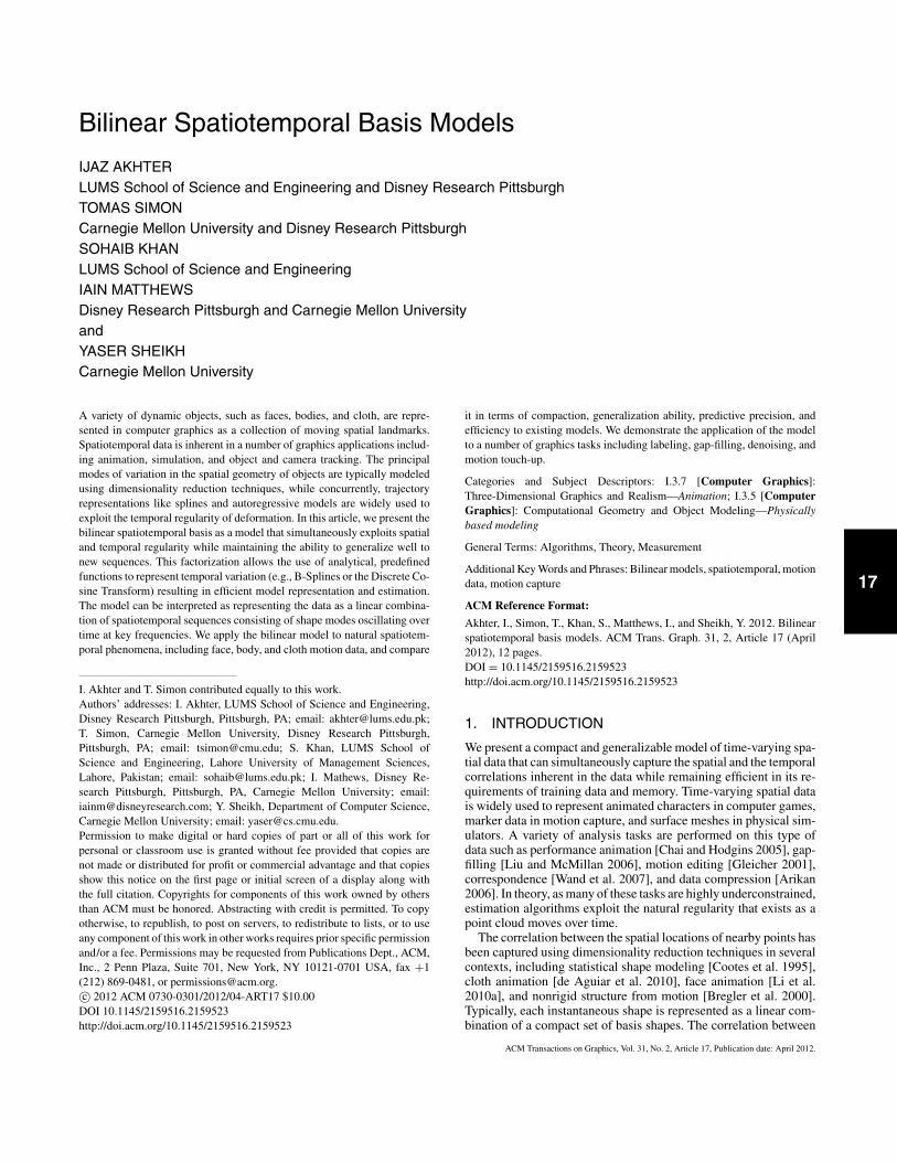
Fig. 1. We present a compact model of spatiotemporal data with the abilityto generalize to unseen data and to accurately predict missing data even whenit is learned from a single training sequence. This figure illustrates the modelbeing used within an expectation maximization routine to simultaneouslyestimate labels for all points in all frames of an unlabeled time-varying pointcloud.

the location of a point at successive time instances has also beenused to compactly represent the motion of a point using autoregres-sive models, via splines [Gleicher 1998], and through dimensional-ity reduction over trajectories [Torresani and Bregler 2002; Akhteret al. 2008]. When dimensionality reduction is used to capture theprincipal modes of variation of the shape geometry, the correlationbetween temporally successive points is ignored; conversely, whendimensionality reduction is performed on trajectories, the correla-tion between spatially adjacent trajectories is ignored. Discardingthese correlations leads to an overparameterization of the data andignores relationships that are useful for performing analysis tasks.

To utilize spatiotemporal regularity, previous research hasproposed directly learning a linear basis that spans the spaceof fixed-duration spatiotemporal sequences [Hamarneh andGustavsson 2004; Min et al. 2009]. As the dimensionality of sucha concatenated linear basis is high, a large amount of training datais required to avoid overfitting, that is, learning spatiotemporalcorrelations that are sequence specific. Filtering approaches, suchas Kalman or particle filters, are also popular approaches to analyzetime-varying spatial data [Thrun et al. 2006]. They represent theinstantaneous configuration of spatial data by state variables andrepresent temporal variation in terms of a dynamical function thatrelates the state at a time instant in terms of the state at the precedingtime instant (or instances). Linear dynamical models are widelyused, and extensions to nonlinear dynamical models (e.g., Wanget al. [2008]) have emerged. Due to the temporally incremental formof dynamical models, they are inherently online models that aredesigned to produce estimates of the state variables as data arrivessequentially.

In this article, we present a new model of time-varying spatialdata as a linear combination of spatiotemporal sequences, each ofwhich may be intuitively interpreted as shape modes oscillatingover time at key frequencies. We demonstrate that such a model canbe expressed in a simple bilinear form, which separately but simul-taneously exploits both the spatial and the temporal regularities thatexist in data. The separation between the spatial and the temporalmodes allows us to condition the model by leveraging analyticaltrajectory bases, such as the Discrete Cosine Transform (DCT) orB-splines. Such conditioning allows the model to generalize wellto sequences of arbitrary length from a small number of trainingsequences while remaining tractable and highly compact. We ana-lyze the form thoroughly, providing bounds on reconstruction errorand experimental validation on four measures of performance: com-paction, generalization ability, computational efficiency, and predic-tive precision. Using these measures we compare our model to linear

dynamical models, shape basis models, splines, trajectory basismodels, and linear spatiotemporal basis models. We demonstratethe broad applicability of the model by directly embedding it instandard algorithms, such as expectation maximization, and per-forming a number of analysis tasks, such as data labeling, denoising,gap-filling, and editing for face, body, and cloth data.

2. RELATED WORK

The representation of time-varying spatial data is a well-studiedproblem in computer graphics, computer vision, and applied math-ematics; an overview of representation and analysis techniques hasbeen covered by Bronstein and colleagues [2008]. A widely usedapproach, due to its simplicity and effectiveness, is to represent thedata as a compact linear combination of basis vectors. PrincipalComponent Analysis (PCA) or a similar dimensionality reductiontechnique is applied to a training set to determine the most signif-icant modes of deformation, and data samples are then describedas a linear combination of these modes. This general approach hassubsequently been extended using nonlinear dimensionality reduc-tion techniques, in particular through the use of kernel methods inKernel PCA [Scholkopf et al. 1997] and Gaussian Process LatentVariable Models (GPLVMs) [Lawrence 2004]. For spatial data, thelinear model is commonly called a point distribution model andwas established through the work of Mardia and Dryden [1989],Le and Kendall [1993], and Cootes and colleagues [1995]. Fortemporal data, dimensionality reduction has also been applied tolearn a compact linear basis of trajectories [Sidenbladh et al. 2000;Torresani and Bregler 2002; Akhter et al. 2008].

Linear models that jointly span both space and time have beenused to track shapes deforming over time and to describe their prin-cipal modes of spatiotemporal variation [Hamarneh and Gustavsson2004], for registration in both space and time [Perperidis et al. 2004],for spatiotemporal segmentation [Mitchell et al. 2002], for motionsynthesis [Urtasun et al. 2004; Min et al. 2009], and for denoising[Lou and Chai 2010]. Typically, joint spatiotemporal models area direct application of linear dimensionality reduction where eachspatiotemporal sequence is vectorized and represents one sample.These models are often specific to the particular sequence lengththat was chosen during training and correlations between pointsat different space-time locations are explicitly learned. These cor-relations are most prominent in periodic motions. To generalizebeyond specific spatiotemporal correlations, joint linear spatiotem-poral models therefore require a large training set, as we show inthis article.

Multilinear methods have been used in a number of computergraphics applications, including expression retargeting [Chuangand Bregler 2005; Vlasic et al. 2005], approximating multi-arrayvisual data [Wang et al. 2005], factoring temporal variationsfrom time-lapse videos [Sunkavalli et al. 2007], and representingtextures [Vasilescu and Terzopoulos 2004]. Min and colleaguesused a multilinear motion model to synthesize, edit, and retargetmotion styles and identities [Min et al. 2010]. Bilinear modelshave been applied to separate style and content by Tenenbaumand Freeman [2000] and have been applied to cardiac data byHoogendoorn and colleagues [2009]. The principal difference isthat while Tenenbaum and Freeman’s symmetric model factorsthe coefficients into bilinear style and content terms which arecombined by a shared mixing basis, our model factors the basisinto spatial and temporal variations and unifies the coefficients.Restating, the Tenenbaum and Freeman approach computes bilinearfactorizations of the coefficients of each sample, while our model islinear in coefficients and a bilinear factorization of the basis. From a


Bilinear Spatiotemporal Basis Models • 17:3

practical perspective, this switch allows for least squares estimationof the coefficients rather than requiring nonlinear iterative mini-mization. When conditioned using a predefined trajectory basis, ourapproach also allows a closed-form solution for model estimation.From a conceptual perspective, our form, when conditioned usingDCT, encodes a spatiotemporal sequence as a linear combinationof spatial modes of variation oscillating at key frequencies.

This interpretation of our bilinear model also finds empiricalsupport in studies of receptive field dynamics [DeAngelis et al.1995] and biological motion [Troje 2002; Sigal et al. 2010], wherea similar sine-wave decomposition of the PCA modes was shownto capture the most prominent features of human gaits. The DCTtrajectory basis has also proven useful in nonrigid structure frommotion [Akhter et al. 2008; Gotardo and Martinez 2011]. In particu-lar, Gotardo and Martinez impose a DCT basis on shape coefficientsto model smooth object deformations. This representation can beexpressed in terms of the bilinear model presented in this article.

Time-varying spatial data has also been modeled as a dynamicalsystem, where a fixed rule describes transitions across time[Thrun et al. 2006]. Compared to basis representations, dynamicalsystems model the evolution of a process as transitions betweentime-steps, making them especially attractive for online processing.Conversely, because it is a model of the process rather than adirect model of the data, operations affecting the entire sequenceare usually more costly. Li and colleagues [2009] model markertrajectories as a Linear Dynamical System (LDS) to infer missingmarkers. Nonlinear dynamical systems have also been successfullyapplied to motion data, most notably Gaussian Process DynamicalModels (GPDMs) [Wang et al. 2008], which have been shown to bean excellent model for synthesis and inference. The main drawbackof Gaussian process models is significant computational and mem-ory cost, making them impractical for very large datasets. Inferenceis usually iterative in the case of missing data. Model estimationis costly as well, and typically accomplished using a nonlinearoptimization (expectation-maximization) that requires adequateinitialization. In comparison, these operations have efficientclosed-form solutions for our DCT-conditioned bilinear model.

From an application perspective, spatiotemporal models are of in-terest in analyzing, editing, synthesizing, compressing, and denois-ing time-varying spatial data. For motion capture data in particular,missing markers, occlusions, and broken trajectories are often sig-nificant issues, and spatiotemporal models are used to infer markerdata across long occlusions and during dropouts. For full-body mo-tion capture applications, the models used often constrain spatialvariation using an articulated skeletal model [Herda et al. 2001;Hornung et al. 2005], or bone-length constraints incorporated intoan LDS framework [Li et al. 2010b]. The focus of this work is onspatial data where an articulated model is not appropriate, such asdense facial motion capture, where most of the motion is due tononrigid deformations. A data-driven approach is that of Liu andMcMillan [2006], who learn piece-wise linear models from largedatasets of motion capture examples for inference. Other work inmotion capture of skin deformations includes Park and Hodgins[2006] and Anguelov and colleagues [2005] who use sparse motioncapture supplemented by a detailed skin model to label and im-pute missing data. Current practice in the industry is for animationhouses to employ motion capture clean-up professionals who createa marker-set, label the points, reconstruct the missing points, andfinally retouch the data, smoothing out noisy points.

Spatiotemporal representations have also been considered for thetasks of motion editing and motion adaptation. Methods relatedto spacetime constraints [Witkin and Kass 1988] aim to globallymodify the character motion to meet certain requirements; these

a1

a2

ω3ω2ω1

f1 f2 f3

p1

p2

Linear Shape BasisLinear Trajectory BasisLinear Spatiotemporal BasisLinear Dynamical ModelBilinear Spatiotemporal Basis

c

cT

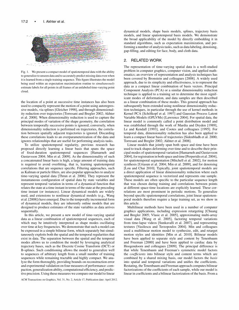
Fig. 2. Graphical model showing parameter dependencies for various mod-els of time-varying spatial data. In this figure, pi refers to a particular pointindex, fi refers to a particular time frame, ωi is a shape coefficient at timefi , and ai is a trajectory coefficient associated with pi . c is a coefficientof a linear spatiotemporal basis, and c is a coefficient of the bilinear spa-tiotemporal basis. T refers to the transition matrix of a linear dynamicalsystem.

methods commonly aim to produce physically realistic motions byminimizing an energy function. Most approaches focus on carefullyformulating the optimization function to enforce the characteristicsof spatiotemporal data and not on the representation itself. Typi-cally, the representation is based on keyframe interpolation of jointangles (for articulated characters) or rig parameters (for facial an-imation). For body motion, a related approach is the per-frame in-verse kinematics + filtering method of Gleicher [2001], who offersan extensive review of this method and related techniques. Otherapproaches to motion transformation use dimensionality reductionin the configuration space of the character to constrain the motionoptimization process [Safonova et al. 2004; de Aguiar et al. 2010],or to match the parameters of a rig [Lewis and Anjyo 2010].

3. METHOD

The time-varying structure of a set of P points sampled at F timeinstances can be represented as a concatenated sequence of 3Dpoints:

SF×3P =

⎡⎢⎣

X11 . . . X1

P

......

XF1 . . . XF

P

⎤⎥⎦ , (1)

where Xij = [

Xij , Y

ij , Z

ij

]denotes the 3D coordinates of the j -

th point at the i-th time instance,1 denoted by one of the graynodes in Figure 2. Thus, the time-varying structure matrix S con-tains 3FP parameters. This representation of the structure is anoverparametrization because it does not take into account the highdegree of regularity generally exhibited by motion data.

One way to exploit the regularity in spatiotemporal data is torepresent the 3D shape at each time instance2 as a linear combinationof a small number of shape basis vectors bj weighted by coefficients

1As a matter of standard notation, we indicate row-index as superscript andcolumn-index as subscript.2The rigid component of deformation is typically compensated for usingProcrustes analysis [Dryden and Mardia 1998]. For clarity of exposition, wedo not include the transformation explicitly in our development.



ωij [Cootes et al. 1995; Bregler et al. 2000],

si =∑

j

ωij bT

j . (2)

Thus, the complete structure matrix, S, which is a row-wise con-catenation of F 3D shapes, can be represented as

S = �BT , (3)

where B is a 3P × Ks matrix containing Ks shape basis vectors,each representing a 3D structure of length 3P , and � is an F × Ks

matrix containing the corresponding shape coefficients ωij , shown

as orange nodes in Figure 2 representing all points at a particulartime frame. The number of shape basis vectors used to represent aparticular instance of motion data is Ks ≤ min{F, 3P }.

An alternate representation of the time-varying structure is tomodel it in the trajectory subspace, as a linear combination of tra-jectory basis vectors θ i [Torresani and Bregler 2002; Akhter et al.2008],

sj =∑

i

aj

i θ i , (4)

where aj

i is the coefficient weighting each trajectory basis vector(denoted by a green node in Figure 2 representing a particularpoint across all frames). In this case, the structure matrix S may beconsidered as the column-wise concatenation of P 3D trajectories,as

S = �AT , (5)

where � is an F × Kt matrix containing Kt trajectory basis as itscolumns, and A is a 3P ×Kt matrix of trajectory coefficients. Here,Kt ≤ min{F, 3P } is the number of trajectory basis vectors spanningthe trajectory subspace. Note that if orthonormal bases are used inboth representations, then BT B = IKs×Ks

and �T � = IKt ×Kt,

because the basis vectors are arranged along the columns of B and�.

3.1 Bilinear Spatiotemporal Basis

The key insight of this article is the observation that using a shapebasis or a trajectory basis independently fails to exploit the fullrange of generalizable spatiotemporal regularities. In the shape ba-sis representation, the temporal regularity of trajectories is ignored;removing temporal regularity by shuffling the frames in time to arandom arrangement only results in a corresponding shuffling of thecoefficients. The same is true for the trajectory basis representation,in which case each spatial location is treated independently; hence,their spatial ordering becomes immaterial. Thus, both representa-tions are overparameterizations because they do not capitalize oneither the spatial or the temporal regularity.

This article presents a bilinear representation of S linking bothshape and trajectory bases in a single model.

THEOREM 1. If S can be expressed exactly as S = �BT andalso S = �AT , then there exists a factorization

S = �CBT , (6)

where C = �T � = AT B is a Kt × Ks matrix of spatiotemporalcoefficients.3

3For clarity, Theorems 1 and 2 are stated assuming orthogonal bases. Equiv-alent proofs for nonorthogonal bases can be derived by using the pseudo-inverses of � and B instead of transposes.

PROOF. Equating the two forms of S in Eqs. (3) and (5), it fol-lows that AT = �T �BT . Substituting this into Eq. (5) yieldsS = ��T �B, where we define C = �T �. The same resultcan be derived in a dual fashion for �, yielding C = AT B.

Eq. (6) describes the bilinear spatiotemporal basis, which con-tains both shape and trajectory bases linked together by a commonset of coefficients. These coefficients can be visualized in two equiv-alent ways as indicated by the two definitions of C given before:(1) C = �T � implies the projection of shape coefficients � ontothe trajectory basis, �, and (2) C = AT B implies the projection oftrajectory coefficients A onto the shape basis B.

For an intuitive understanding of the bilinear spatiotemporalmodel, consider the coefficient ci

j at the i-th row and the j -th col-umn in C (denoted by the red node in Figure 2). This coefficientrepresents the weight of the outer product of the i-th trajectory basisvector, θ i , and the j -th shape basis vector, bj . This outer productwill result in a time-varying structure sequence in which all pointsof a single shape mode (as defined by the j -th shape basis) willvary over time (as defined by the i-th trajectory basis). The sum ofall such outer products θ ibT

j , weighted by the corresponding coef-ficient, ci

j , results in the bilinear representation of S, equivalent toEq. (6).

S =∑

i

∑j

cijθ ibT

j (7)

This is best illustrated as an animation of each shape basis vectorbj modulated over time according to each trajectory basis vectorθ i , as shown in the accompanying video (in the vignette titled “Bi-linear Spatiotemporal Modes”). Under our bilinear basis model,spatiotemporal data is represented as a linear combination of eachof these modulated spatiotemporal sequences.

3.2 Bounds on Reconstruction Error

In Theorem 1, the bilinear spatiotemporal model is derived forthe case of perfect representation of time-varying structure. Wecan also use the bilinear basis (Eq. (6)) with a reduced number ofbasis vectors. In the following theorem, we describe bounds on thebilinear spatiotemporal model error as a function of approximationerrors of the shape and trajectory models.

THEOREM 2. If the reconstruction error of the trajectory modelis εt = ‖S − �AT ‖F , and the error of the shape model is εs =‖S − �BT ‖F , then the error of the bilinear spatiotemporal modelε = ‖S−�CBT ‖F is upper bounded by εt + εs and lower boundedby max(εt , εs), where ‖ · ‖F is the Frobenius norm.

PROOF. The approximate model may be expressed as

S = �AT + �⊥A⊥T , (8)

S = �BT + �⊥B⊥T , (9)

where the columns of �⊥ and B⊥ form a basis for the nullspaces of�T and BT respectively. A⊥T and �⊥ are the coefficients of thesenullspaces. Here εt = ‖�⊥A⊥T ‖F and εs = ‖�⊥B⊥T ‖F . SettingEqs. (8) and (9) equal and noting �T �⊥ = 0 we get

S = �CBT + ��T �⊥B⊥T + �⊥A⊥T . (10)

By inspection we see that ε = ‖��T �⊥B⊥T + �⊥A⊥T ‖F . Fromthe triangle inequality we get ε ≤ ‖��T �⊥B⊥T ‖F + εt . As ��T

is an orthogonal projection matrix onto the range of �, it followsthat ‖��T �⊥B⊥T ‖ ≤ ‖�⊥B⊥T ‖ = εs . Therefore, ε ≤ εt + εs . Adual equality can be written where ε = ‖�⊥A⊥T BBT + �⊥B⊥T ‖



can be derived. As ε must be greater than εs and εt it follows thatε ≥ max(εt , εs).

Theorem 2 states that the bilinear spatiotemporal model errorcannot exceed the sum of errors of the shape and trajectory models.This error, however, is reached with far fewer coefficients for thebilinear model as compared to the shape or trajectory models; thisparsimony will be demonstrated in Section 3.6.

3.3 Comparison with Linear Spatiotemporal Basis

It is instructive to compare the bilinear spatiotemporal basis witha linear spatiotemporal representation. In the latter case, S is vec-torized into a single column vector which can be represented by alinear spatiotemporal basis

vec (S) = �c, (11)

where vec(S) is a column-wise vectorized version of S, � is a3FP×K matrix representing K linear spatiotemporal basis vectors,and c is a K ×1 column vector of coefficients (denoted by the whitenode in Figure 2). We can write the bilinear spatiotemporal basis asa linear model

vec (S) = (B ⊗ �) vec (C) , (12)

where ⊗ denotes the Kronecker Product [Jain 1989]. Hence, for Ks

shape and Kt trajectory bases in the bilinear model, an equivalentlinear model will have K = KsKt columns in �. Note, however,that not all linear spatiotemporal basis can be factored into bilinearspatiotemporal basis.

While the linear and the bilinear spatiotemporal models canmodel both spatial and temporal regularity, linear spatiotemporalbases will need substantial amounts of data to generalize beyondsequence-specific correlations. The linear basis learns any correla-tion within the fixed spatiotemporal window, whereas the bilinearbasis must be separable. This becomes crucial when learning fromsequences that are not temporally aligned, for example, facial mo-tion from utterances of different speech content.

3.4 Conditioned Bilinear Bases

We observe that while appropriate shape basis will often have tobe learned to suit particular datasets,4 the high degree of temporalsmoothness in natural motions allows a predefined analytical trajec-tory basis to be used for a wide variety of datasets without signifi-cant loss in representation. The conditioned bilinear spatiotemporalrepresentation is thus a special case of Eq. (6),

S = �CBT + ε, (13)

where � contains the first Kt vectors of the predefined trajectorybasis arranged along its columns, each of length F . The ability touse a predefined trajectory basis yields closed-form and numericallystable solutions, for both the estimation of the shape basis andcoefficients in Eq. (6). The benefit of using a trajectory basis forwhich an analytical expression exists is that the same model canrepresent time-varying structures of arbitrary durations.

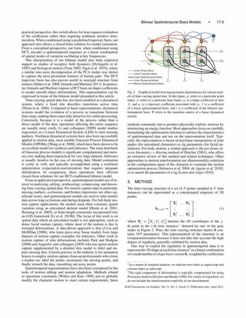
A particularly suitable choice of a conditioning trajectory basisis the Discrete Cosine Transform (DCT) basis. Figure 3 showsthat the optimal PCA basis learned from a large number of variedfacial motion capture sequences converges to the DCT basis. This

4In some cases using a predefined shape basis may be possible. Examplesinclude character animation, where blendshapes may be artist defined, orphysical simulations where an analytical shape basis may be obtained.

DCT

PCA 10

PCA 100

PCA 1000

Fig. 3. For large training sets of natural motion (including nonperiodicmotion), the PCA-learned trajectory basis approaches DCT. Ordered left-to-right, top-to-bottom, comparison of the first 10 DCT basis vectors (orange)with the first 10 data-specific PCA trajectory basis vectors learned on avarying number of facial motion capture training sequences: 10 sequences(light gray), 100 sequences (dark gray), and 1000 sequences (black). Eachsequence and each vector depicted here is 100 frames in length.

result is consistent with Akhter and colleagues [2010] who havedemonstrated a similar experiment for human body sequences, andwith Arikan [2006] who uses the DCT basis to compress motion-capture data. Indeed, it is well known that the DCT basis approachesthe optimal PCA basis if the data is generated from a stationary first-order Markov process [Rao and Yip 1990]. Given the high temporalregularity present in almost all human motions, it is not surprisingthat we empirically find DCT to be an excellent basis for trajectoriesof varied types.

Other choices of a conditioning trajectory basis are possible andmay be preferable in specific applications. While DCT shows com-paction that is close to optimal, the support of each basis vector isglobal and each coefficient affects the entire sequence. This may beundesirable in some cases, and therefore overlapped-block versionssuch as the modified DCT are often used in online signal processingtasks. A practical alternative with localized basis support is the B-spline basis [Deboor 1978], commonly used to approximate smoothfunctions while offering local control over the shape of the curve.The B-spline basis is not orthogonal, which results in a slightlymore expensive solution for estimating the coefficients, as will beshown in Section 3.5.

Using a predefined trajectory basis is a major strength of thebilinear representation, which not only reduces the complexity ofestimating bilinear bases to being nearly identical to shape-onlymodels, but also provides good generalization capabilities, and theability to handle sequences of arbitrary duration. In contrast, forthe linear spatiotemporal model given in Eq. (11), the spatial andthe temporal components do not factor out separately, and hence itis not possible to use a predefined basis for one mode of variationand a data-driven basis for the other.

3.5 Parameter Estimation

An important strength of the conditioned bilinear model is thatthe estimation of coefficients and basis have closed-form solutionsrequiring only linear least squares and SVD routines. Hence, the es-timation is efficient, optimal, and numerically stable. Learning thebilinear basis given a set of example sequences has been studied forthe more general cases of bilinear and multilinear models [Magnusand Neudecker 1999]. While several competing tensor decomposi-tions exist, one possibility is to iteratively project and take the SVDin each of the two subspaces, analogous to the process of estimatingthe bilinear coefficients Tenenbaum and Freeman [2000]. Another



option is to stack the sequences as a third-order tensor and factorizeit using Higher-Order SVD (HOSVD), a generalization of SVD fortensors. However, the conditioned bilinear representation results insimplified estimation, because in this case one of the three matricesin the model is already known. In the following subsections, wefirst discuss the problem of computing the coefficients, C, givenknown bases � and B. Subsequently, in Section 3.5.2 we addressthe problem of estimating the shape basis.

3.5.1 Estimating the Coefficients of a Bilinear Model. Givena shape basis B and a trajectory basis �, we wish to compute thebilinear model coefficients C, that minimize the reconstruction errorfor a given S.

The solution may be estimated by minimizing the squared recon-struction error

C = arg minC

∣∣∣∣(S − �CBT)∣∣∣∣2

F(14)

For any bases � and B, the general solution for optimal C is interms of the pseudo-inverses

C = �+S(BT

)+, (15)

where superscripted + denotes the Moore-Penrose pseudo-inverse.For the case when both � and B have full column-rank, the pre-ceding solution is unique. If the bases are orthogonal, then thesolution simplifies to C = �T SB, which implies simply projectingthe structure S onto each of the bases sequentially. This simplifica-tion applies to the DCT basis, but not to the B-spline basis, sincethat basis is not orthonormal.

3.5.2 Conditioned Shape Basis Estimation. While HOSVD oriterative SVD may be used to estimate bilinear bases in general,the estimation of the conditioned bilinear bases is significantly sim-pler. This is because the trajectory basis are already known. Hence,given a set of training examples, the appropriate shape basis for theconditioned bilinear model may be estimated using the followingtheorem.

THEOREM 3. Given a trajectory basis � and a set of trainingsequences of time-varying structure, S1, S2, . . . , SN , the optimalshape basis which minimizes the squared reconstruction error isgiven by the row-space computed through SVD of the matrix

� = [ST

1 , ST2 , . . . , ST

N

]T, (16)

where Si = ��+Si denotes the reconstruction of S from its trajec-tory projection.

PROOF. For one sequence, expanding S into its components thatspan the trajectory basis and its null space, the optimal shape basisminimizes

arg minB

‖��+S + �⊥A⊥T − ��+S(BT )+BT ‖2F . (17)

Observing that, for a fixed �, �⊥A⊥T does not depend on the choiceof B, then the optimal rank-Ks orthogonal B can be computed asthe row space of S via SVD. For more than one structure sequence,the optimal shape basis B will result from the SVD of the matrixformed by stacking the sequences Si into an FN × 3P matrix �,defined before. The error to be minimized is equivalent to ||� −�(BT )+BT ||2F .

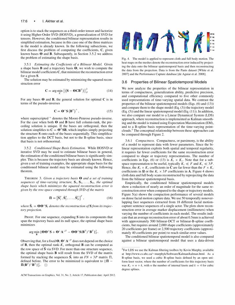
Fig. 4. The model is applied to represent cloth and full body motion. Theheat maps on the meshes denote the reconstruction error induced by project-ing the data onto the bilinear spatiotemporal basis and then reconstructingthe data from the projection. Data is from the Pants dataset [White et al.2007] and the Performance Capture database [de Aguiar et al. 2008].

3.6 Properties of Bilinear Spatiotemporal Models

We now analyze the properties of the bilinear representation interms of compactness, generalization ability, predictive precision,and computational efficiency compared to five other commonlyused representations of time-varying spatial data. We contrast theproperties of the bilinear spatiotemporal models (Eqs. (6) and (13))and compare them to the shape model (Eq. (3)) the trajectory model(Eq. (5)) and the linear spatiotemporal model (Eq. (11)). In addition,we also compare our model to a Linear Dynamical System (LDS)approach, where reconstruction is implemented as Kalman smooth-ing and the model is trained using Expectation Maximization (EM),and to a B-spline basis representation of the time-varying point-clouds.5 The conceptual relationship between these approaches canbe compared through Figure 2.

3.6.1 Compactness. Compactness, or parsimony, is the abilityof a model to represent data with fewer parameters. Since the bi-linear representation exploits both spatial and temporal regularity,it requires far fewer coefficients for the same reconstruction errorcompared to shape or trajectory representations. The number ofcoefficients in Eqs. (6) or (13) is Kt × Ks . Note that for a sub-space representation to be useful, typically Kt � F and Ks � 3P .Hence, the Kt × Ks coefficients in C are far fewer than the F × Ks

coefficients in � or the Kt × 3P coefficients in A. Figure 4 showscloth data and full body scans reconstructed by reprojecting the datafrom the bilinear spatiotemporal basis.

Empirically, the conditioned bilinear spatiotemporal modelsshow a reduction of nearly an order of magnitude for the same re-construction error when compared to the shape or trajectory models.Figure 5(a) shows the compaction performance of several modelson dense facial motion capture data. We use 50 temporally nonover-lapping face sequences extracted from 18 different facial motion-capture sentence sequences of a single actor. The plots show recon-struction error in average marker displacement (millimeters) whenvarying the number of coefficients in each model. The results indi-cate that an average reconstruction error of about 0.5mm is achievedwith approximately 500 bilinear-DCT or bilinear-B-spline coeffi-cients, but requires around 2,000 shape coefficients (approximately20 coefficients per frame) or 2,500 trajectory coefficients (approxi-mately 40 coefficients per point) to reach similar error values.

The conditioned bilinear spatiotemporal model is also comparedagainst a bilinear spatiotemporal model that uses a data-driven

5For LDS we use the Kalman filtering toolbox by Kevin Murphy, availableat http://www.cs.ubc.ca/∼murphyk/Software/Kalman/kalman.html. As aB-spline basis, we used a cubic B-spline basis defined by an open uni-form knot vector, where the number of coefficients for this trajectory basiswas Kt = n + k, with n the number of internal knots and k = 4 for cubicdegree splines.



0.0 0.5 1.0 1.5 2.0 2.5 3.00

0.2

0.4

0.6

0.8

1

1.2

1.4

1.6

1.8

2

Number of coefficients x1000

Ave

rage

Mar

ker

Err

or (

mm

)

50 sequences, 100 frames per sequence, 63 points per frame

Bilinear (K =K )t s

Bilinear−DCT (K =K )t s

Bilinear−B−Spline (K =K )t s

Shape−PCATrajectory−PCATrajectory−DCTTrajectory−B−SplineLinearLDS

(a) reconstruction error on training data

100

101

102

103

0

0.5

1

1.5

2

2.5

3

3.5

Number of training sequences (log scale)

Ave

rage

mar

ker

erro

r (m

m)

1386 sequences, 96 frames per sequence, 32 points per frame

Bilinear K =18,K =23 (414 coefs)t s

Bilinear−DCT K =18,K =23 (414 coefs)t s

Bilinear B−Spline K =21,K =22 (462 coefs)t s

Shape−PCA K =17 (1632 coefs)s

Trajectory−PCA K=14 (1344 coefs)t

Trajectory−DCT K=14 (1344 coefs)t

Trajectory−B−Spline K=15 (1440 coefs)t

Linear K=129 (129 coefs)LDS K =19 (1824 coefs)

s

(b) generalization error on testing data

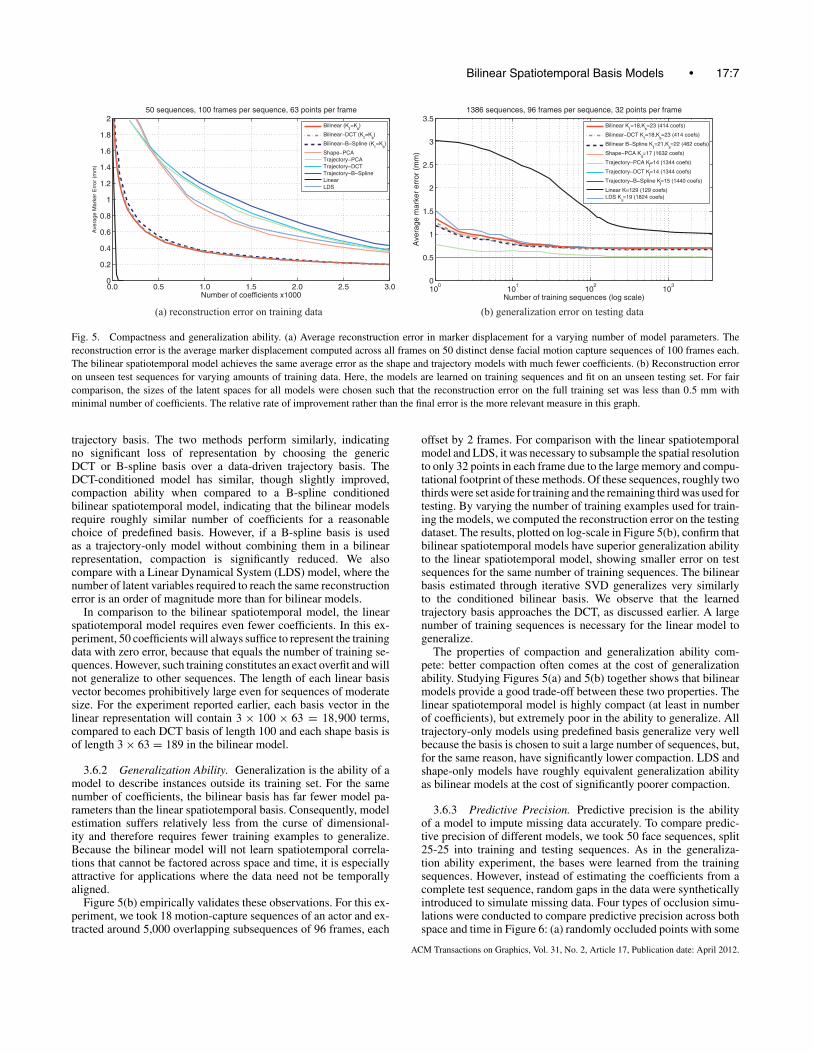
Fig. 5. Compactness and generalization ability. (a) Average reconstruction error in marker displacement for a varying number of model parameters. Thereconstruction error is the average marker displacement computed across all frames on 50 distinct dense facial motion capture sequences of 100 frames each.The bilinear spatiotemporal model achieves the same average error as the shape and trajectory models with much fewer coefficients. (b) Reconstruction erroron unseen test sequences for varying amounts of training data. Here, the models are learned on training sequences and fit on an unseen testing set. For faircomparison, the sizes of the latent spaces for all models were chosen such that the reconstruction error on the full training set was less than 0.5 mm withminimal number of coefficients. The relative rate of improvement rather than the final error is the more relevant measure in this graph.

trajectory basis. The two methods perform similarly, indicatingno significant loss of representation by choosing the genericDCT or B-spline basis over a data-driven trajectory basis. TheDCT-conditioned model has similar, though slightly improved,compaction ability when compared to a B-spline conditionedbilinear spatiotemporal model, indicating that the bilinear modelsrequire roughly similar number of coefficients for a reasonablechoice of predefined basis. However, if a B-spline basis is usedas a trajectory-only model without combining them in a bilinearrepresentation, compaction is significantly reduced. We alsocompare with a Linear Dynamical System (LDS) model, where thenumber of latent variables required to reach the same reconstructionerror is an order of magnitude more than for bilinear models.

In comparison to the bilinear spatiotemporal model, the linearspatiotemporal model requires even fewer coefficients. In this ex-periment, 50 coefficients will always suffice to represent the trainingdata with zero error, because that equals the number of training se-quences. However, such training constitutes an exact overfit and willnot generalize to other sequences. The length of each linear basisvector becomes prohibitively large even for sequences of moderatesize. For the experiment reported earlier, each basis vector in thelinear representation will contain 3 × 100 × 63 = 18,900 terms,compared to each DCT basis of length 100 and each shape basis isof length 3 × 63 = 189 in the bilinear model.

3.6.2 Generalization Ability. Generalization is the ability of amodel to describe instances outside its training set. For the samenumber of coefficients, the bilinear basis has far fewer model pa-rameters than the linear spatiotemporal basis. Consequently, modelestimation suffers relatively less from the curse of dimensional-ity and therefore requires fewer training examples to generalize.Because the bilinear model will not learn spatiotemporal correla-tions that cannot be factored across space and time, it is especiallyattractive for applications where the data need not be temporallyaligned.

Figure 5(b) empirically validates these observations. For this ex-periment, we took 18 motion-capture sequences of an actor and ex-tracted around 5,000 overlapping subsequences of 96 frames, each

offset by 2 frames. For comparison with the linear spatiotemporalmodel and LDS, it was necessary to subsample the spatial resolutionto only 32 points in each frame due to the large memory and compu-tational footprint of these methods. Of these sequences, roughly twothirds were set aside for training and the remaining third was used fortesting. By varying the number of training examples used for train-ing the models, we computed the reconstruction error on the testingdataset. The results, plotted on log-scale in Figure 5(b), confirm thatbilinear spatiotemporal models have superior generalization abilityto the linear spatiotemporal model, showing smaller error on testsequences for the same number of training sequences. The bilinearbasis estimated through iterative SVD generalizes very similarlyto the conditioned bilinear basis. We observe that the learnedtrajectory basis approaches the DCT, as discussed earlier. A largenumber of training sequences is necessary for the linear model togeneralize.

The properties of compaction and generalization ability com-pete: better compaction often comes at the cost of generalizationability. Studying Figures 5(a) and 5(b) together shows that bilinearmodels provide a good trade-off between these two properties. Thelinear spatiotemporal model is highly compact (at least in numberof coefficients), but extremely poor in the ability to generalize. Alltrajectory-only models using predefined basis generalize very wellbecause the basis is chosen to suit a large number of sequences, but,for the same reason, have significantly lower compaction. LDS andshape-only models have roughly equivalent generalization abilityas bilinear models at the cost of significantly poorer compaction.

3.6.3 Predictive Precision. Predictive precision is the abilityof a model to impute missing data accurately. To compare predic-tive precision of different models, we took 50 face sequences, split25-25 into training and testing sequences. As in the generaliza-tion ability experiment, the bases were learned from the trainingsequences. However, instead of estimating the coefficients from acomplete test sequence, random gaps in the data were syntheticallyintroduced to simulate missing data. Four types of occlusion simu-lations were conducted to compare predictive precision across bothspace and time in Figure 6: (a) randomly occluded points with some



70 75 80 85 90 95

1

2

3

4

5

6

% Points Missing

Pre

dict

ion

erro

r (m

m)

Completely Invisible Trajectories=20

BilinearBilinear DCTBilinear B SplinesShape PCALinearLDS

(a) spatial imputation

30 40 50 60 70 80 90

1

2

3

4

5

6

% Points Missing

Pre

dict

ion

erro

r (m

m)

Completely Invisible Frames=20

BilinearBilinear DCTBilinear B SplinesTrajectory PCATrajectory DCTTrajectory B SplineLinearLDS

(b) temporal imputation

65 70 75 80 85 90 950

1

2

3

4

5

6

% Points Missing

Pre

dict

ion

erro

r (m

m)

Invisible Trajectories=20, Invisible Frames=20

BilinearBilinear DCTBilinear B SplinesLinearLDS

(c) spatiotemporal imputation

10 20 30 40 50 60

1

2

3

4

5

6

Gap Length

Pre

dict

ion

erro

r (m

m)

BilinearBilinear DCTBilinear B SplinesShape PCATrajectory PCATrajectory DCTTrajectory B SplineLinearLDS

(d) clustered imputation

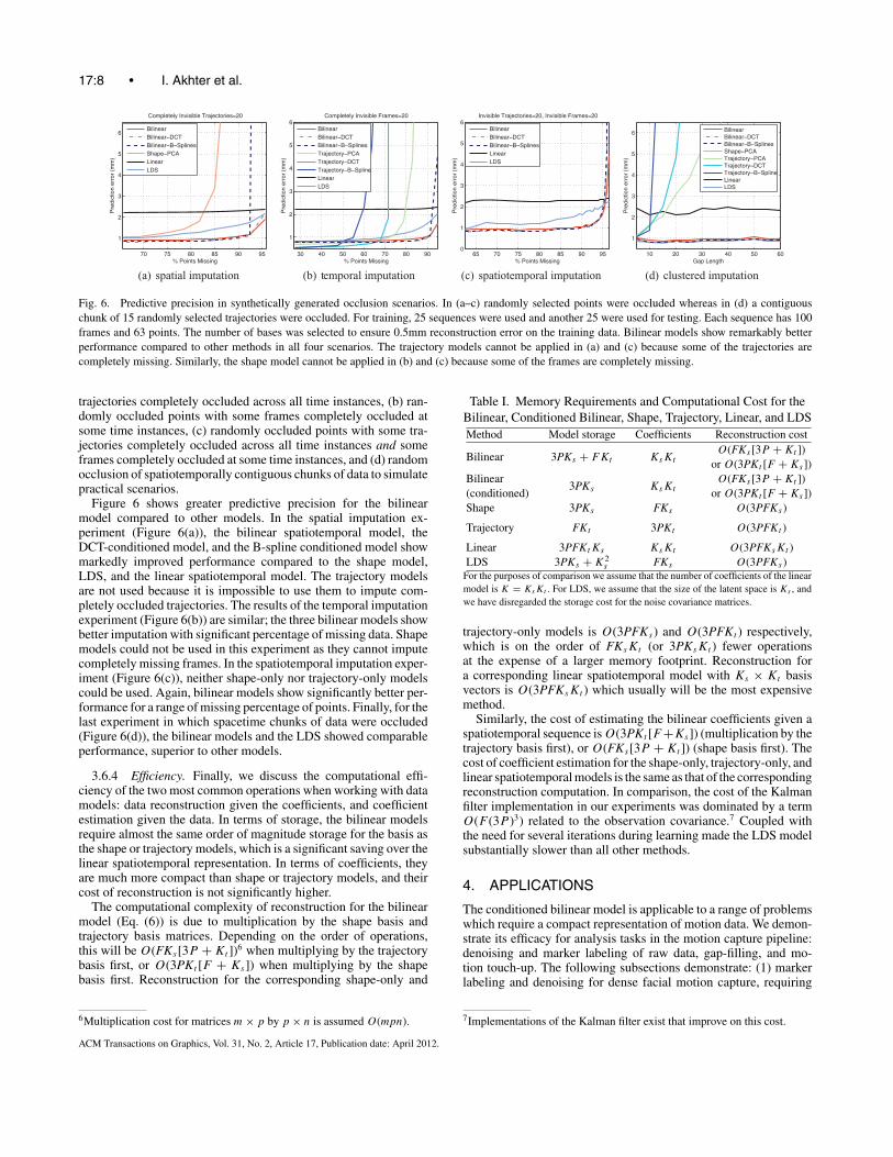
Fig. 6. Predictive precision in synthetically generated occlusion scenarios. In (a–c) randomly selected points were occluded whereas in (d) a contiguouschunk of 15 randomly selected trajectories were occluded. For training, 25 sequences were used and another 25 were used for testing. Each sequence has 100frames and 63 points. The number of bases was selected to ensure 0.5mm reconstruction error on the training data. Bilinear models show remarkably betterperformance compared to other methods in all four scenarios. The trajectory models cannot be applied in (a) and (c) because some of the trajectories arecompletely missing. Similarly, the shape model cannot be applied in (b) and (c) because some of the frames are completely missing.

trajectories completely occluded across all time instances, (b) ran-domly occluded points with some frames completely occluded atsome time instances, (c) randomly occluded points with some tra-jectories completely occluded across all time instances and someframes completely occluded at some time instances, and (d) randomocclusion of spatiotemporally contiguous chunks of data to simulatepractical scenarios.

Figure 6 shows greater predictive precision for the bilinearmodel compared to other models. In the spatial imputation ex-periment (Figure 6(a)), the bilinear spatiotemporal model, theDCT-conditioned model, and the B-spline conditioned model showmarkedly improved performance compared to the shape model,LDS, and the linear spatiotemporal model. The trajectory modelsare not used because it is impossible to use them to impute com-pletely occluded trajectories. The results of the temporal imputationexperiment (Figure 6(b)) are similar; the three bilinear models showbetter imputation with significant percentage of missing data. Shapemodels could not be used in this experiment as they cannot imputecompletely missing frames. In the spatiotemporal imputation exper-iment (Figure 6(c)), neither shape-only nor trajectory-only modelscould be used. Again, bilinear models show significantly better per-formance for a range of missing percentage of points. Finally, for thelast experiment in which spacetime chunks of data were occluded(Figure 6(d)), the bilinear models and the LDS showed comparableperformance, superior to other models.

3.6.4 Efficiency. Finally, we discuss the computational effi-ciency of the two most common operations when working with datamodels: data reconstruction given the coefficients, and coefficientestimation given the data. In terms of storage, the bilinear modelsrequire almost the same order of magnitude storage for the basis asthe shape or trajectory models, which is a significant saving over thelinear spatiotemporal representation. In terms of coefficients, theyare much more compact than shape or trajectory models, and theircost of reconstruction is not significantly higher.

The computational complexity of reconstruction for the bilinearmodel (Eq. (6)) is due to multiplication by the shape basis andtrajectory basis matrices. Depending on the order of operations,this will be O(FKs[3P + Kt ])6 when multiplying by the trajectorybasis first, or O(3PKt [F + Ks]) when multiplying by the shapebasis first. Reconstruction for the corresponding shape-only and

6Multiplication cost for matrices m × p by p × n is assumed O(mpn).

Table I. Memory Requirements and Computational Cost for theBilinear, Conditioned Bilinear, Shape, Trajectory, Linear, and LDSMethod Model storage Coefficients Reconstruction cost

Bilinear 3PKs + FKt KsKtO(FKs [3P + Kt ])

or O(3PKt [F + Ks ])Bilinear

3PKs KsKtO(FKs [3P + Kt ])

(conditioned) or O(3PKt [F + Ks ])Shape 3PKs FKs O(3PFKs )

Trajectory FKt 3PKt O(3PFKt )

Linear 3PFKtKs KsKt O(3PFKsKt )LDS 3PKs + K2

s FKs O(3PFKs )For the purposes of comparison we assume that the number of coefficients of the linearmodel is K = KsKt . For LDS, we assume that the size of the latent space is Ks , andwe have disregarded the storage cost for the noise covariance matrices.

trajectory-only models is O(3PFKs) and O(3PFKt ) respectively,which is on the order of FKsKt (or 3PKsKt ) fewer operationsat the expense of a larger memory footprint. Reconstruction fora corresponding linear spatiotemporal model with Ks × Kt basisvectors is O(3PFKsKt ) which usually will be the most expensivemethod.

Similarly, the cost of estimating the bilinear coefficients given aspatiotemporal sequence is O(3PKt [F +Ks]) (multiplication by thetrajectory basis first), or O(FKs[3P + Kt ]) (shape basis first). Thecost of coefficient estimation for the shape-only, trajectory-only, andlinear spatiotemporal models is the same as that of the correspondingreconstruction computation. In comparison, the cost of the Kalmanfilter implementation in our experiments was dominated by a termO(F (3P )3) related to the observation covariance.7 Coupled withthe need for several iterations during learning made the LDS modelsubstantially slower than all other methods.

4. APPLICATIONS

The conditioned bilinear model is applicable to a range of problemswhich require a compact representation of motion data. We demon-strate its efficacy for analysis tasks in the motion capture pipeline:denoising and marker labeling of raw data, gap-filling, and mo-tion touch-up. The following subsections demonstrate: (1) markerlabeling and denoising for dense facial motion capture, requiring

7Implementations of the Kalman filter exist that improve on this cost.



Fig. 7. Point clouds reconstructed from motion capture systems usuallysuffer broken trajectories and mislabeled points. The figure shows frames56, 84, 100, 320, and 560 of a motion capture session (first row), rawmotion capture data (second row), and our labeling results (third row). Astime progresses, errors propagate and more points are mislabeled. Imageused with permission of Elizabeth Carter.

just a few minutes of cleanup compared to the current standardof several hours of professional time, (2) gap-filling and imputa-tion on face sequences given appropriately learned bases, and (3) amotion touch-up tool which allows plausible deformations of anentire motion capture sequence by moving only a few points andwithout employing any kinematic or skeletal model. Each of theseapplications exploits the DCT-conditioned bilinear model.

4.1 Motion Capture Labeling and Denoising

Reconstruction using motion capture systems often requires te-dious postprocessing for data cleanup, to connect broken trajec-tories, impute missing markers, correct mislabeled markers, anddenoise trajectories, as illustrated in Figure 7. We have developed asemiautomatic tool which simultaneously labels, denoises and im-putes missing points, and drastically reduces the time required forcleanup while generating reconstructions qualitatively and quantita-tively similar to those by industry professionals. The process oftengenerates error-free labels, but when it does not, our semiauto-mated tool allows a few user-identified corrections to automaticallypropagate temporally, hence reducing cleanup time. Our approachis based on using the DCT-conditioned bilinear representation tocompute marker labels. Given the bases, the bilinear coefficientsand marker labels are interdependent and are iteratively estimatedusing an Expectation Maximization (EM) algorithm.

4.1.1 Expectation Maximization. We model the marker datausing the DCT-conditioned bilinear basis. The observed 3D co-ordinates of the pth marker in frame f is Xp

f = Xp

f + e, where

e ∼ N (0, σ 2I) is measurement error, and Xp

f is the true value of Xp

f

and σ denotes the standard deviation of the error. We want to assigna label l

p

f ∈ {1, . . . , P } to each marker Xp

f associating it to a uniquetrajectory, such that the rearranged matrix S = �CBT . The goal ofthe EM algorithm is to estimate both the set of hidden variables l

p

f

as well as the model parameters, C and σ .

0 0.5 1 1.5 2 2.50

0.2

0.4

0.6

0.8

1

Reconstruction error (mm)

CD

F

JR Sen127JE Sen87DC ROMJE Sen28EB facs79LE ROMJE ROMLiz K2KB ROM

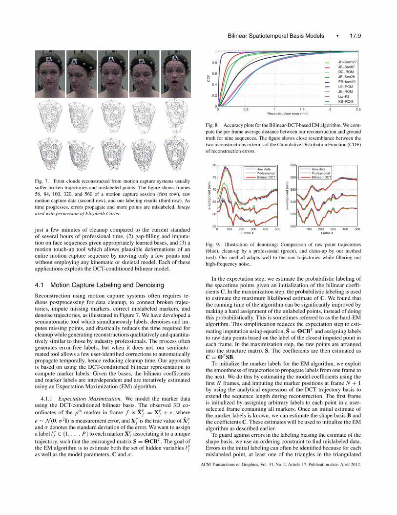
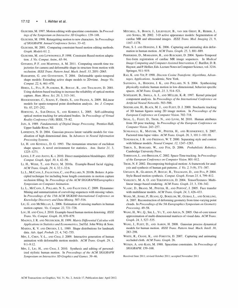
Fig. 8. Accuracy plots for the Bilinear-DCT-based EM algorithm. We com-pute the per frame average distance between our reconstruction and groundtruth for nine sequences. The figure shows close resemblance between thetwo reconstructions in terms of the Cumulative Distribution Function (CDF)of reconstruction errors.

0 100 200 300 400 50055

60

65

70

75

80

Frame #

xco

mpo

nent

(m

m)

Raw dataProfessionalBilinear DCT

100 200 300 400 500500

520

540

560

580

600

Frame #

yco

mpo

nent

(m

m)

Raw dataProfessionalBilinear DCT

Fig. 9. Illustration of denoising: Comparison of raw point trajectories(blue), clean-up by a professional (green), and clean-up by our method(red). Our method adapts well to the raw trajectories while filtering outhigh-frequency noise.

In the expectation step, we estimate the probabilistic labeling ofthe spacetime points given an initialization of the bilinear coeffi-cients C. In the maximization step, the probabilistic labeling is usedto estimate the maximum likelihood estimate of C. We found thatthe running time of the algorithm can be significantly improved bymaking a hard assignment of the unlabeled points, instead of doingthis probabilistically. This is sometimes referred to as the hard-EMalgorithm. This simplification reduces the expectation step to esti-mating imputation using equation, S = �CBT and assigning labelsto raw data points based on the label of the closest imputed point ineach frame. In the maximization step, the raw points are arrangedinto the structure matrix S. The coefficients are then estimated asC = �T SB.

To initialize the marker labels for the EM algorithm, we exploitthe smoothness of trajectories to propagate labels from one frame tothe next. We do this by estimating the model coefficients using thefirst N frames, and imputing the marker positions at frame N + 1by using the analytical expression of the DCT trajectory basis toextend the sequence length during reconstruction. The first frameis initialized by assigning arbitrary labels to each point in a user-selected frame containing all markers. Once an initial estimate ofthe marker labels is known, we can estimate the shape basis B andthe coefficients C. These estimates will be used to initialize the EMalgorithm as described earlier.

To guard against errors in the labeling biasing the estimate of theshape basis, we use an ordering constraint to find mislabeled data.Errors in the initial labeling can often be identified because for eachmislabeled point, at least one of the triangles in the triangulated


17:10 • I. Akhter et al.In

pu

t P

oin

t1%

of

tota

l po

ints

Imp

ute

d D

ata

1mm

2mm

3mm

4mm

5mm

Frame 150 Frame 250 Frame 350 Frame 450

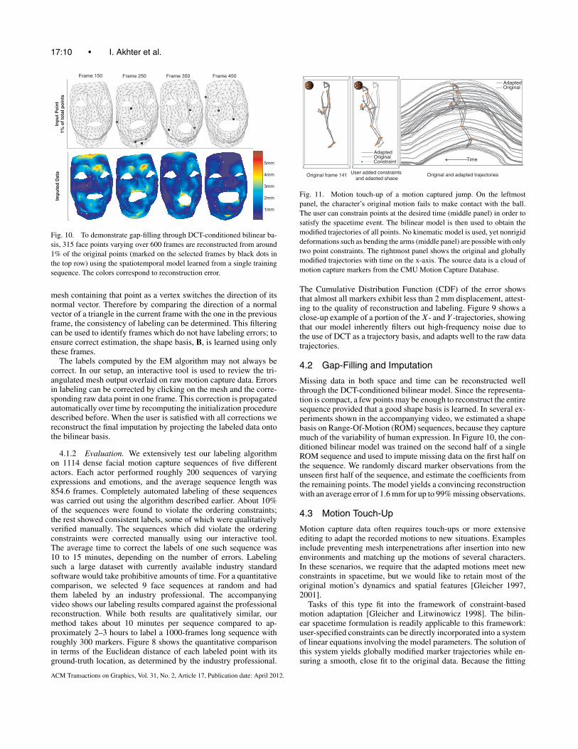
Fig. 10. To demonstrate gap-filling through DCT-conditioned bilinear ba-sis, 315 face points varying over 600 frames are reconstructed from around1% of the original points (marked on the selected frames by black dots inthe top row) using the spatiotemporal model learned from a single trainingsequence. The colors correspond to reconstruction error.

mesh containing that point as a vertex switches the direction of itsnormal vector. Therefore by comparing the direction of a normalvector of a triangle in the current frame with the one in the previousframe, the consistency of labeling can be determined. This filteringcan be used to identify frames which do not have labeling errors; toensure correct estimation, the shape basis, B, is learned using onlythese frames.

The labels computed by the EM algorithm may not always becorrect. In our setup, an interactive tool is used to review the tri-angulated mesh output overlaid on raw motion capture data. Errorsin labeling can be corrected by clicking on the mesh and the corre-sponding raw data point in one frame. This correction is propagatedautomatically over time by recomputing the initialization proceduredescribed before. When the user is satisfied with all corrections wereconstruct the final imputation by projecting the labeled data ontothe bilinear basis.

4.1.2 Evaluation. We extensively test our labeling algorithmon 1114 dense facial motion capture sequences of five differentactors. Each actor performed roughly 200 sequences of varyingexpressions and emotions, and the average sequence length was854.6 frames. Completely automated labeling of these sequenceswas carried out using the algorithm described earlier. About 10%of the sequences were found to violate the ordering constraints;the rest showed consistent labels, some of which were qualitativelyverified manually. The sequences which did violate the orderingconstraints were corrected manually using our interactive tool.The average time to correct the labels of one such sequence was10 to 15 minutes, depending on the number of errors. Labelingsuch a large dataset with currently available industry standardsoftware would take prohibitive amounts of time. For a quantitativecomparison, we selected 9 face sequences at random and hadthem labeled by an industry professional. The accompanyingvideo shows our labeling results compared against the professionalreconstruction. While both results are qualitatively similar, ourmethod takes about 10 minutes per sequence compared to ap-proximately 2–3 hours to label a 1000-frames long sequence withroughly 300 markers. Figure 8 shows the quantitative comparisonin terms of the Euclidean distance of each labeled point with itsground-truth location, as determined by the industry professional.

AdaptedOriginal

Original frame 141 User added constraints and adapted shape

Time

Original and adapted trajectories

AdaptedOriginalConstraint

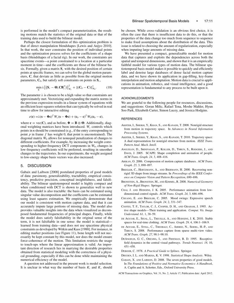
Fig. 11. Motion touch-up of a motion captured jump. On the leftmostpanel, the character’s original motion fails to make contact with the ball.The user can constrain points at the desired time (middle panel) in order tosatisfy the spacetime event. The bilinear model is then used to obtain themodified trajectories of all points. No kinematic model is used, yet nonrigiddeformations such as bending the arms (middle panel) are possible with onlytwo point constraints. The rightmost panel shows the original and globallymodified trajectories with time on the x-axis. The source data is a cloud ofmotion capture markers from the CMU Motion Capture Database.

The Cumulative Distribution Function (CDF) of the error showsthat almost all markers exhibit less than 2 mm displacement, attest-ing to the quality of reconstruction and labeling. Figure 9 shows aclose-up example of a portion of the X- and Y -trajectories, showingthat our model inherently filters out high-frequency noise due tothe use of DCT as a trajectory basis, and adapts well to the raw datatrajectories.

4.2 Gap-Filling and Imputation

Missing data in both space and time can be reconstructed wellthrough the DCT-conditioned bilinear model. Since the representa-tion is compact, a few points may be enough to reconstruct the entiresequence provided that a good shape basis is learned. In several ex-periments shown in the accompanying video, we estimated a shapebasis on Range-Of-Motion (ROM) sequences, because they capturemuch of the variability of human expression. In Figure 10, the con-ditioned bilinear model was trained on the second half of a singleROM sequence and used to impute missing data on the first half onthe sequence. We randomly discard marker observations from theunseen first half of the sequence, and estimate the coefficients fromthe remaining points. The model yields a convincing reconstructionwith an average error of 1.6 mm for up to 99% missing observations.

4.3 Motion Touch-Up

Motion capture data often requires touch-ups or more extensiveediting to adapt the recorded motions to new situations. Examplesinclude preventing mesh interpenetrations after insertion into newenvironments and matching up the motions of several characters.In these scenarios, we require that the adapted motions meet newconstraints in spacetime, but we would like to retain most of theoriginal motion’s dynamics and spatial features [Gleicher 1997,2001].

Tasks of this type fit into the framework of constraint-basedmotion adaptation [Gleicher and Litwinowicz 1998]. The bilin-ear spacetime formulation is readily applicable to this framework:user-specified constraints can be directly incorporated into a systemof linear equations involving the model parameters. The solution ofthis system yields globally modified marker trajectories while en-suring a smooth, close fit to the original data. Because the fitting



is performed in the model’s compact parameterization, the result-ing motions match the statistics of the original data or that of thetraining data used to build the bilinear model.

Perhaps the closest formulation of this optimization problem isthat of direct manipulation blendshapes [Lewis and Anjyo 2010].In that work, the user constrains the position of individual pointsand the optimization process solves for the coefficients of a shapebasis (blendshapes of a facial rig). In our work, the constraints arespacetime events—a point constrained to a location at a particularmoment in time—and the coefficients are those of the bilinear ba-sis. Formally, given a matrix Sc with the desired position of certainpoints at specific frames, we can solve for the global motion param-eters, C, that deviate as little as possible from the original motionparameters, C0, but satisfy soft constraints on points in Sc,

minC

λ∥∥(

Sc − �cCBTc

)∥∥2

Wc+ ‖(C0 − C)‖2

W0. (18)

The parameter λ is chosen to be a high value so that constraints areapproximately met. Vectorizing and expanding the matrix norms inthe previous expression results in a linear system of equations withan efficient least-squares solution that can typically be solved in realtime to allow for interactive editing

e(c) =λ(s − �c)T Wc(s − �c) + (c0 − c)T W0(c0 − c),

where c = vec(C), and as before, � = B ⊗ �. Additionally, diag-onal weighting matrices have been introduced. Wc controls whichpoints in s should be constrained (e.g., if the entry corresponding topoint p in frame f has weight 0, that point is unconstrained). Thediagonal matrix W0 allows for nonequal penalization of changes todifferent coefficients. For example, by increasing the weight corre-sponding to higher-frequency DCT components in W0, changes inlow-frequency coefficients will be preferred, resulting in smootherchanges to the trajectories. In our experiments, the weight assignedto low-energy shape basis vectors was also increased.

5. DISCUSSION

Gabaix and Laibson [2008] postulated properties of good modelsof data: parsimony, generalizability, tractability, empirical consis-tency, predictive precision, conceptual insightfulness, and falsifi-ability. The bilinear spatiotemporal model is highly compact andwhen conditioned with DCT is shown to generalize well to newdata. The model is also tractable: the basis can be estimated usingsingular value decomposition and the coefficients can be estimatedusing least squares estimation. We empirically demonstrate thatour model is consistent with motion capture data, and that it canaccurately impute large portions of missing data. The model alsoprovides valuable insights into the data when visualized as decom-posed fundamental frequencies of principal shapes. Finally, whilethe model does satisfy falsifiability in the original sense of theterm, it is not falsifiable in one sense: the model is statistical—learned from training data—and does not use spacetime physicalconstraints as developed by Witkin and Kass [1988]. For instance, inediting marker positions (see Figure 11), bone length will not nec-essarily be kept constant by this model, nor does the model ensureforce-coherence of the motion. This limitation restricts the usageto touch-ups where the linear approximation is valid. An impor-tant direction of research lies in marrying the desirable propertiesobtained from statistical modeling with the correctness of a physi-cal grounding, especially if this can be done while maintaining thenumerical efficiency of the model.

A question not addressed in the present work is model selection.It is unclear in what way the number of basis Kt and Ks should

be chosen. While cross-validation is an obvious first choice, it isoften the case that there is insufficient data to do this, or that theproperties of the data change too much from sequence to sequenceto make fixed assumptions about the distribution of the data. Thisissue is related to choosing the amount of regularization, especiallywhen imputing large amounts of missing data.

We have presented a compact, generalizable model for motiondata that captures and exploits the dependencies across both thespatial and temporal dimensions, and shown that it is an empiricallyfaithful model for various types of motion data. The bilinear spa-tiotemporal basis model makes it possible to quickly and efficientlylabel and denoise large databases of dense facial motion capturedata, and we have shown its application in gap-filling, key-frameinterpolation and motion adaptation. Motion data is crucial to appli-cations in animation, robotics, and visual intelligence, and a goodrepresentation is fundamental to any process to be built upon it.

ACKNOWLEDGMENTS

We are grateful to the following people for resources, discussions,and suggestions: Goran Milic, Rafael Tena, Moshe Mahler, HyunSoo Park, Elizabeth Carter, Simon Lucey, and Jessica Hodgins.

REFERENCES

AKHTER, I., SHEIKH, Y., KHAN, S., AND KANADE, T. 2008. Nonrigid structurefrom motion in trajectory space. In Advances in Neural InformationProcessing Systems.

AKHTER, I., SHEIKH, Y., KHAN, S., AND KANADE, T. 2010. Trajectory space:A dual representation for nonrigid structure from motion. IEEE Trans.Pattern Anal. Mach. Intell.

ANGUELOV, D., SRINIVASAN, P., KOLLER, D., THRUN, S., RODGERS, J., AND

DAVIS, J. 2005. SCAPE: Shape completion and animation of people.ACM Trans. Graph. 24, 3, 408–416.

ARIKAN, O. 2006. Compression of motion capture databases. ACM Trans.Graph. 25, 3, 890–897.

BREGLER, C., HERTZMANN, A., AND BIERMANN, H. 2000. Recovering non-rigid 3D shape from image streams. In Proceedings of the IEEE Confer-ence on Computer Vision and Pattern Recognition, 690–696.

BRONSTEIN, A., BRONSTEIN, M., AND KIMMEL, R. 2008. Numerical Geometryof Non-Rigid Shapes. Springer.

CHAI, J. AND HODGINS, J. K. 2005. Performance animation from low-dimensional control signals. ACM Trans. Graph. 24, 3, 686–696.

CHUANG, E. AND BREGLER, C. 2005. Mood swings: Expressive speechanimation. ACM Trans. Graph. 24, 2, 331–347.

COOTES, T. F., TAYLOR, C. J., COOPER, D. H., AND GRAHAM, J. 1995. Ac-tive shape models—Their training and application. Comput. Vis. ImageUnderstand. 61, 1, 38–59.

DE AGUIAR, E., SIGAL, L., TREUILLE, A., AND HODGINS, J. K. 2010. Stablespaces for real-time clothing. ACM Trans. Graph. 29, 4, 106:1–106:9.

DE AGUIAR, E., STOLL, C., THEOBALT, C., AHMED, N., SEIDEL, H.-P., AND

THRUN, S. 2008. Performance capture from sparse multi-view video.ACM Trans. Graph. 27, 98:1–98:10.

DEANGELIS, G. C., OHZAWA, I., AND FREEMAN, R. D. 1995. Receptive-field dynamics in the central visual pathways. Trends Neurosci. 18, 10,451–458.

DEBOOR, C. 1978. A Practical Guide to Splines. Springer.

DRYDEN, I. L. AND MARDIA, K. V. 1998. Statistical Shape Analysis. Wiley.

GABAIX, X. AND LAIBSON, D. 2008. The seven properties of good models.In The Foundations of Positive and Normative Economics: A Handbook,A. Caplin and A. Schotter, Eds., Oxford University Press.



GLEICHER, M. 1997. Motion editing with spacetime constraints. In Proceed-ings of the Symposium on Interactive 3D Graphics. 139–148.

GLEICHER, M. 1998. Retargetting motion to new characters. In Proceedingsof SIGGRAPH. Annual Conference Series. 33–42.

GLEICHER, M. 2001. Comparing constraint-based motion editing methods.Graph. Models 63, 2.

GLEICHER, M. AND LITWINOWICZ, P. 1998. Constraint-Based motion adapta-tion. J. Vis. Comput. Anim., 65–94.

GOTARDO, P. F. AND MARTINEZ, A. M. 2011. Computing smooth time tra-jectories for camera and deformable shape in structure from motion withocclusion. IEEE Trans. Pattern Anal. Mach. Intell. 33, 2051–2065.

HAMARNEH, G. AND GUSTAVSSON, T. 2004. Deformable spatio-temporalshape models: Extending active shape models to 2D+time. Image Vis.Comput. 22, 6, 461–470.

HERDA, L., FUA, P., PLANKERS, R., BOULIC, R., AND THALMANN, D. 2001.Using skeleton-based tracking to increase the reliability of optical motioncapture. Hum. Move. Sci. 20, 3, 313–341.

HOOGENDOORN, C., SUKNO, F., ORDES, S., AND FRANGI, A. 2009. BiLinearmodels for spatio-temporal point distribution analysis. Int. J. Comput.Vis. 85, 237–252.

HORNUNG, A., SAR-DESSAI, S., AND KOBBELT, L. 2005. Self-calibratingoptical motion tracking for articulated bodies. In Proceedings of VirtualReality Conference (VR). IEEE, 75–82.

JAIN, A. 1989. Fundamentals of Digital Image Processing. Prentice-Hall,Upper Saddle River, NJ.

LAWRENCE, N. D. 2004. Gaussian process latent variable models for visu-alisation of high dimensional data. In Advances in Neural InformationProcessing Systems.

LE, H. AND KENDALL, D. G. 1993. The riemannian structure of euclideanshape spaces: A novel environment for statistics. Ann. Statist 21, 3,1225–1271.

LEWIS, J. P. AND ANJYO, K.-I. 2010. Direct manipulation blendshapes. IEEEComput. Graph. Appl. 30, 4, 42–50.

LI, H., WEISE, T., AND PAULY, M. 2010a. Example-Based facial rigging.ACM Trans. Graph. 29, 4, 32:1–32:6.

LI, L., MCCANN, J., FALOUTSOS, C., AND POLLARD, N. 2010b. Bolero: A prin-cipled technique for including bone length constraints in motion captureocclusion filling. In Proceedings of the ACM SIGGRAPH/EurographicsSymposium on Computer Animation.

LI, L., MCCANN, J., POLLARD, N. S., AND FALOUTSOS, C. 2009. Dynammo:Mining and summarization of coevolving sequences with missing values.In Proceedings of the 15th ACM SIGKDD International Conference onKnowledge Discovery and Data Mining. 507–516.

LIU, G. AND MCMILLAN, L. 2006. Estimation of missing markers in humanmotion capture. Vis. Comput. 22, 721–728.

LOU, H. AND CHAI, J. 2010. Example-based human motion denoising. IEEETrans. Vis. Comput. Graph. 16, 870–879.

MAGNUS, J. R. AND NEUDECKER, H. 1999. Matrix Differential Calculus withApplications in Statistics and Econometrics, 2nd Ed. John Wiley & Sons.

MARDIA, K. V. AND DRYDEN, I. L. 1989. Shape distributions for landmarkdata. Adv. Appl. Probab. 21, 4, 742–755.

MIN, J., CHEN, Y.-L., AND CHAI, J. 2009. Interactive generation of humananimation with deformable motion models. ACM Trans. Graph. 29, 1,9:1–9:12.

MIN, J., LIU, H., AND CHAI, J. 2010. Synthesis and editing of personal-ized stylistic human motion. In Proceedings of the ACM SIGGRAPHSymposium on Interactive 3D Graphics and Games. 39–46.

MITCHELL, S., BOSCH, J., LELIEVELDT, B., VAN DER GEEST, R., REIBER, J.,AND SONKA, M. 2002. 3-D active appearance models: Segmentation ofcardiac MR and ultrasound images. IEEE Trans. Med. Imaging 21, 9,1167–1178.

PARK, S. I. AND HODGINS, J. K. 2006. Capturing and animating skin defor-mation in human motion. ACM Trans. Graph. 25, 3, 881–889.

PERPERIDIS, D., MOHIADDIN, R., AND RUECKERT, D. 2004. Spatio-Temporalfree-form registration of cardiac MR image sequences. In MedicalImage Computing and Computer-Assisted Intervention, C. Barillot, D. R.Haynor, and P. Hellier, Eds. Lecture Notes in Computer Science, vol. 3216.Springer, 911–919.

RAO, K. AND YIP, P. 1990. Discrete Cosine Transform: Algorithms, Advan-tages, Applications. Academic, New York.

SAFONOVA, A., HODGINS, J. K., AND POLLARD, N. S. 2004. Synthesizingphysically realistic human motion in low-dimensional, behavior-specificspaces. ACM Trans. Graph. 23, 3, 514–521.

SCHOLKOPF, B., SMOLA, A. J., AND MULLER, K.-R. 1997. Kernel principalcomponent analysis. In Proceedings of the International Conference onArtificial Neural Networks. 583–588.

SIDENBLADH, H., BLACK, M. J., AND FLEET, D. J. 2000. Stochastic trackingof 3D human figures using 2D image motion. In Proceedings of theEuropean Conference on Computer Vision. 702–718.

SIGAL, L., FLEET, D., TROJE, N., AND LIVNE, M. 2010. Human attributesfrom 3D pose tracking. In Proceedings of the European Conference onComputer Vision. 243–257.

SUNKAVALLI, K., MATUSIK, W., PFISTER, H., AND RUSINKIEWICZ, S. 2007.Factored time-lapse video. ACM Trans. Graph. 26, 3, 101:1–101:10.

TENENBAUM, J. B. AND FREEMAN, W. T. 2000. Separating style and contentwith bilinear models. Neural Comput. 12, 1247–1283.

THRUN, S., BURGARD, W., AND FOX, D. 2006. Probabilistic Robotics.Cambridge University Press.

TORRESANI, L. AND BREGLER, C. 2002. Space-Time tracking. In Proceedingsof the European Conference on Computer Vision. 801–812.

TROJE, N. F. 2002. Decomposing biological motion: A framework for anal-ysis and synthesis of human gait patterns. J. Vis. 2, 5 (9), 371–387.

URTASUN, R., GLARDON, P., BOULIC, R., THALMANN, D., AND FUA, P. 2004.Style-Based motion synthesis. Comput. Graph. Forum 23, 4, 799–812.

VASILESCU, M. A. O. AND TERZOPOULOS, D. 2004. TensorTextures: Multi-linear image-based rendering. ACM Trans. Graph. 23, 3, 336–342.

VLASIC, D., BRAND, M., PFISTER, H., AND POPOVIC, J. 2005. Face transferwith multilinear models. ACM Trans. Graph. 24, 3, 426–433.

WAND, M., JENKE, P., HUANG, Q., BOKELOH, M., GUIBAS, L., AND SCHILLING,A. 2007. Reconstruction of deforming geometry from time-varying pointclouds. In Proceedings of the 5th Eurographics Symposium on GeometryProcessing. 49–58.

WANG, H., WU, Q., SHI, L., YU, Y., AND AHUJA, N. 2005. Out-of-core tensorapproximation of multi-dimensional matrices of visual data. ACM Trans.Graph. 24, 3, 527–535.

WANG, J., FLEET, D., AND AARON, H. 2008. Gaussian process dynamicalmodels for human motion. IEEE Trans. Pattern Anal. Mach. Intell. 30,283–298.

WHITE, R., CRANE, K., AND FORSYTH, D. 2007. Capturing and animatingoccluded cloth. ACM Trans. Graph. 26.

WITKIN, A. AND KASS, M. 1988. Spacetime constraints. In Proceedings ofSIGGRAPH. 159–168.

Received June 2011; revised October 2011; accepted November 2011


bilinear spatiotemporal basis models - computer...

Documents