GENOMICS 41, 141–154 (1997)ARTICLE NO. GE974652

Binning Clones by Hybridization with Complex Probes: StatisticalRefinement of an Inner Product Mapping Method

CHRIS ANDREWS,* B. DEVLIN,*,†,1 MARK PERLIN,‡ AND KATHRYN ROEDER*

*Department of Statistics and ‡Department of Computer Science, Carnegie Mellon University; and †Department of Psychiatry,University of Pittsburgh Medical Center, Pittsburgh, Pennsylvania 15213

Received June 18, 1996; accepted January 24, 1997

tent mapping (Green and Green, 1991) with megaYACsMolecular methods that use long-range information (Bellanne-Chantelot et al., 1992) was used to establish

to solve genomics problems (i.e., top-down strategies) local proximity groups for new STS markers and toefficiently have become increasingly prominent in the locate these groups relative to the premapped frame-genomics literature. One such method, an implementa- work markers. Without the top-down long-range infor-tion of inner product mapping (IPM), uses noisy, long- mation, the bottom-up information provided by STS-range radiation hybrid (RH)/YAC overlap data and rel- content mapping would yield little more than rough,atively noise-free RH/STS overlap data to localize local clusters.clones to specific chromosomal regions. Because the The STS framework map will be extremely useful formolecular data are rarely noise-free, statistical models

cloning disease genes and as a foundation for large-tailored to the top-down molecular methods make thescale sequencing efforts. However, the map itself willmethods far more effective. We develop two statisticalbe insufficient to complete the next goal of the humanmodels for IPM (or any other top-down strategy of sim-genome project, determining the entire nucleotide se-ilar form), a parametric logit model and a nonparamet-quence, even if it achieves a much higher STS density.ric order-restricted model, and show how these modelsOther sequencing resources will be needed, particu-can be implemented within a hierarchical Bayeslarly smaller, sequenceable clones such as BACs orframework. Using these models, we refine the chromo-PACs localized to specific genomic regions.some 11 map reported in M. Perlin et al. (1995, Geno-

mics 28: 315–327). Our analyses improve the IPM map, Localization of BACs or PACs could be achieved byboth in terms of successful localization of clones and any of a large number of methods. One top-downin terms of the confidence with which they are local- method that could accomplish this task, dubbed IPMized. q 1997 Academic Press for inner product mapping (Perlin and Chakravarti,

1993), was used by Perlin et al. (1995) to develop a YACmap of chromosome 11. This method shares features

INTRODUCTION with the STS-framework mapping methodology in thateach uses long-range information for efficient localiza-Top-down strategies, which divide a large, difficult tion and each utilizes both noisy and relatively noise-problem into smaller, simpler subproblems or which free data. A fundamental difference between the meth-use long-range information to simplify the problem ods is the definition of the bins and what is binned. For(Aho et al., 1983), play an increasingly prominent role the framework map, the bins are defined by chromo-in genomics research. The process by which the se-somal breaks, specifically recombinant, RH, and mega-quence-tag site (STS) framework map of the humanYAC breaks, and it is the STSs themselves that aregenome was built (Hudson et al., 1995) provides anbinned (Cox et al., 1994). For IPM, bins are chromo-excellent illustration of a top-down strategy. The goalsomal regions surrounding STSs, and it is the clonesof this mapping effort was to locate STS markers onthemselves that are binned. While different in philoso-specific human chromosomes and, within chromo-phy, these two methods are clearly complementary.somes, determine their order and approximate loca-

IPM uses two kinds of data to achieve its binning.tions. To map about 15,000 STS markers, two long-For a set of STSs and RHs, RH versus PCR STS com-range resources were employed: radiation hybrid (RH)parisons (Cox et al., 1990) generate data to position themapping of monomorphic STSs and genetic mappingfragments of each RH; statistically, each experimentof polymorphic STSs. Together, these methods mappedyields an indicator describing whether the STS and RHabout 70% of the markers, which then function as aoverlap. For a library of clones and the same set offramework on which to hang new markers. STS-con-RHs, the RHs are serially hybridized against the setof clones (Monaco et al., 1991) to generate data that1 To whom correspondence should be addressed. Telephone: (412)

268-8973. Fax: (412) 268-7828. E-mail: bdevlin@stat.cmu.edu. position RHs relative to each clone; statistically, each

1410888-7543/97 $25.00

Copyright q 1997 by Academic PressAll rights of reproduction in any form reserved.

AID GENO 4652 / 6r2f$$$261 03-15-97 00:54:29 gnmal

ANDREWS ET AL.142

into a series of far smaller, simpler experiments canmake a molecular task more feasible, top-down strate-gies pave the way for more efficient and stable statisti-cal analyses by reducing the problem to a simpler setof subproblems.

In this report, we refine the chromosome 11 mapreported in Perlin et al. (1995). To accomplish this task,we develop statistical methods to complement IPM orany other top-down method of similar structure. Theobjective of these methods is to assign YAC (or smaller-insert bacterial) clones to local chromosomal regionscentered by STS locations (‘‘STS bins’’) based on theoverlap characteristics of a set of RHs with both theclones and the STSs. The likelihood model is incorpo-rated into Bayesian hierarchical models (Berger, 1985),which provides a convenient framework for expressingthe likelihood results in terms of the probability thata given clone is from each STS bin. Powerful computa-tional methods that are available within this Bayesianframework are obtained to determine these probabili-ties. Finally, the clone map is evaluated using indepen-dent, clone–clone hybridization data (Qin et al., 1996).

FIG. 1. Pictoral representation of IPM method. (a) An example MOLECULAR METHODSof the true clone locations along the chromosome. Note that clones2 and 4 do not overlap any STS. (b) The two idealized data tables: With a very dense STS map, clone binning can be achieved bytable A records the overlap (1) or nonoverlap (0) results of the YAC directly comparing each clone against each STS. Instead, for greatervs RH comparisons; table B records the (1/0) results of the RH vs experimental efficiency, Perlin et al. (1995) implemented an IPMSTS comparisons. (c) The clone localization table obtained by com- approach (Perlin and Chakravarti, 1993) to obtain the desired bin-paring rows of table A and columns of table B. Note that clones 2 ning. Specifically, Perlin et al. (1995) binned chromosome 11-specificand 4 are correctly localized to STS bins near their true locations. YAC clones using two datasets: a dataset containing an RH signature

for each clone, obtained by DNA hybridization studies, and a datasetcontaining an RH signature for each mapped STS, obtained by PCRexperiment ideally yields an indicator describing comparison. These data, the clone versus RH table and the RH versus

whether the clone and RH overlap. The key idea of IPM mapped STS table, were then computationally combined to indirectlyis straightforward when these indicators of overlap are infer each clone’s location relative to the mapped STSs.

Because we analyze the same data that Perlin et al. (1995) usedconsidered: If the set of RHs that overlap an STS alsoto produce their chromosome 11 map, we only outline their molecularappear to overlap a specific clone, then the clone’s truemethods. Refer to the original paper for more details.location on the chromosome is most likely proximate

The clone versus RH table. The clones Perlin et al. (1995) mappedto that STS (Fig. 1). were the Roswell Park Cancer Institute (RPCI) library of 1728 non-The molecular results are less than ideal, however. chimeric chromosome 11 YACs, which have a 350-kb average insert

size (Qin et al., 1996). To produce the clone versus RH table, theyAlthough the STS versus RH data are almost noise-robotically spotted Alu-PCR products of chromosome 11 YACs ontofree, there is usually substantial uncertainty aboutnylon membranes, then serially hybridized these against Alu-PCRwhether a clone and an RH overlap. In this instance,products from RHs, which are described below. The results of thesean experimental result for clone versus RH overlap is experiments were scores, at one of five levels, indicating the probabil-

commonly scored on a scale such as from 02, for un- ity of RH/clone overlap. Only the 1295 clones that obtained at leastone probable RH/clone overlap were used in our analyses.likely to overlap, to 2, for very likely to overlap. The

The RH versus mapped STS table. The complex probes used byIPM study of Perlin et al. (1995) successfully used L2Perlin et al. (1995) were a collection of 73 chromosome 11-derivedminimization (L2-min) to compare the RH scores ofradiation hybrids (Richard et al., 1991, 1993), having an 8-Mb aver-clones and STSs, in part to overcome this data uncer-age interbreak distance, an average retention probability of 0.25,

tainty. This L2-min implementation has limitations, and a minimum retention probability of 0.02. These RHs had beenhowever, which include limited probabilistic interpre- previously characterized by a set of 506 chromosome 11-specific STSs

(James et al., 1994), demonstrating 240 unique RH bins and an aver-tation of the map and less than maximal efficiency.age interbin distance of 625 kb. The binary comparison scores of theThese limitations can be overcome naturally by build-73 RHs versus the 240 bins had been used to map the STSs (Jamesing a statistical model that dovetails with IPM’s top- et al., 1994), and also served to localize the chromosomal fragments

down strategy. of each RH relative to the mapped STSs.In fact, there can be a synergism between top-down This methodology differs from the more typical protocol by which

simple probes are hybridized against more complex immobilized tar-strategies and statistical methods that is very appeal-gets. To reduce the number of experiments significantly, IPM drawsing. Top-down strategies can turn potentially intracta-on Lehrach’s idea (Monaco et al., 1991) of reversing the hybridizationble statistical problems into problems that are easily direction and using complex probes derived from inter-Alu-PCR (Nel-

solved by powerful statistical methods. In the same son et al., 1989) products of RH DNA. When such complex DNAprobes are used, there are at least four potential problems. First,way that changing a single, very complex experiment

AID GENO 4652 / 6r2f$$$262 03-15-97 00:54:29 gnmal

STATISTICAL METHODS FOR BINNING CLONES 143

the inter-Alu amplification of the complex DNA may be incomplete Basic Notationdue to PCR competition between its many inter-Alu sites; this leadsto underrepresentation of the inter-Alu sites in the probe and can For notation, let i Å 1, . . . , I index the clones; j Å 1,cause false-negative scores. Second, because any one target has few . . . , J index the STSs; and k Å 1, . . . , K index the RHs.inter-Alu sites, and the labeled probe may have thousands of sites For the chromosome 11 dataset, I Å 1295, J Å 240, and(only a few of which are specific for the target), there is a potential

K Å 73. Also, let tables A, B, and C represent the truesignal-to-noise problem in detecting true hybridizations. Third, be-state of nature: Aik Å 1 if clone i and RH k overlap, andcause a target can present a variable number of sites, and the com-

plex probe may show large variation in amplification, labeling, and 0 otherwise; Bkj Å 1 if RH k and STS j overlap, and 0binding of these sites, the observed hybridization intensities can ex- otherwise; CijÅ 1 if AikÅ Bkj for each k, and 0 otherwisehibit large variation. Fourth, repetitive genomic DNA in the complex (Fig. 1).probe may cause false-positive scores.

We wish to estimate table C from estimates of tablesNone of these obstacles is insurmountable, as the results of Perlinet al. (1995) show: A and B. For each i we assume Cij Å 1 for exactly one

value of j and we can therefore write Ci Å j to denote1. Because the false-negative rate exceeded 50%, the inter-Alu ‘‘clone i is in STS bin j.’’ This assumption is reasonable,competition did appear to reduce inter-Alu site representation in

provided that clones are sufficiently small, STSs arethe complex probe. However, computational methods separated thenot too dense, and RHs are sufficiently large. Thesesignal from the noise in these data.

2. The inherently low signal-to-noise ratio required the use of techniques are robust to minor violations of these as-larger amounts of radioactive label to provide useful data. sumptions. Note that Ci Å j does not imply that clone

3. The variability of inter-Alu hybridization generated a wide i and STS j overlap. It merely implies that any RH thatrange of intensities on the autoradiographs. By using a quantitativeoverlaps with clone i also overlaps with STS j and viceas opposed to a binary scoring scale, however, the data were de-

scribed adequately. In these data, both true and false DNA overlaps versa.could produce identical hybridization signals; thus, the observed in-tensity can only be interpreted probabilistically. Observable Variables

4. The repetitive DNA was suppressed by competing the labeledprobe with an excess of Cot-1 DNA and by including placental DNA The analyses of the chromosome 11 dataset assumein the prehybridization solution. Since the hybridization data has a that table B is measured error free, except for 80 miss-low false-positive rate, genomic repeats did not appear to pose a ing values. This simplifying assumption is reasonablesubstantial problem.

because the RH versus STS overlap experiments arevery reliable. A value in B is referred to as the ‘‘overlap

STATISTICAL ANALYSES status’’ between an RH and an STS. We handle themissing values using standard statistical techniques(Tanner and Wong, 1987) described in the appendices.The objective is to estimate the (posterior) probabil-

ity that a clone should be assigned to a particular STS Table A cannot be determined without error due touncertainty in scoring the overlap between a clone andbin (that is, the short chromosomal region surrounding

an STS). To obtain this probability, two items are re- an RH. For each clone i and each RH k, the experi-menter estimates the possibility of overlap using a dis-quired: a prior probability distribution for the bin of

the clone and the likelihood of each bin based on the crete scale ranging from 1 (very unlikely) to L (verylikely). An entry in this I 1 K table of estimates, A, isdata (Berger, 1985). For this application and most ap-

plications of this kind, there is little a priori informa- referred to as the ‘‘overlap score’’ (or just ‘‘score’’) be-tween a clone and an RH. Modeling this scoring processtion about the clone’s true position in the genome. For

this reason we use distributions that give each bin is a key feature of our analysis.For the chromosome 11 dataset, A has no missingequal weight, a priori. Where other priors are required,

we use distributions that are dominated by the likeli- observations, and each score is one of five levels. Be-cause very few of the highest scores were observed, thehood and hence have little influence on the outcome of

the analysis. fourth and fifth categories are collapsed into a singlecategory (so L Å 4).Bayesian models have been used successfully for

other genomic applications. Lange and Boehnke (1992), The average score (over the K RHs) for a given clonevaries widely by clone for these data. Some of the varia-for example, used Bayesian methods for RH mapping.

Although such models are analytically daunting, they tion is due to the number of times the clone overlaps theRHs. In the chromosome 11 dataset, the RH coverage ofare still tractable by applying powerful computational

machinery. Because the models we propose are too com- the chromosome is not uniform: 61 of the 73 RHs over-lap the STS bin 89 (centromere); only 12 overlap STSplex for direct analysis, we use a Markov chain Monte

Carlo algorithm (Geyer, 1989; Gelfand and Smith, bin 196. However, this nonuniform coverage does notexplain all the variability in the average clone scores1990; Smith and Roberts, 1993) to generate an estimate

of the posterior distribution of the bin of each clone. (see Molecular Methods). Thus we build a probabilitymodel with parameters that vary by clone, thereby ac-Where appropriate, each of the following subsections

begins with a general explanation of the methods de- counting for the clonal variation and making the modelmore accurate. For a given clone the probability ofscribed therein and then proceeds to give technical sup-

porting matter. The main ideas of the methodology achieving a given score is assumed to be the same forany RH that overlaps that clone. The same assumptionshould be apparent without thorough consideration of

the technical matter. is made for RHs that do not overlap the clone.

AID GENO 4652 / 6r2f$$$262 03-15-97 00:54:29 gnmal

ANDREWS ET AL.144

with the given STS for each score versus the givenclone.

The pattern in this table determines how well theith row of A matches the jth column of B. If the clonehas been placed in the correct STS bin, high scores inA should be concentrated in the RH/STS overlap rowand low scores should be concentrated in the RH/STSnonoverlap row. For example, Table 2 displays two

FIG. 2. Data for a hypothetical example. Table A contains over- such tables from the chromosome 11 dataset, one whenlap score for clone i (rows) vs RH k (columns). It is a noisy estimate clone 1B5 is placed in bin 103 (Table 2a) and the otherof table A in Fig. 1. Table B contains the overlap status between RH when clone 1B5 is placed in bin 31 (Table 2b). Notek (rows) and STS j (columns). It is observed without error.

that Table 2a has most observations in the high-scorecolumns of the overlap row and in the low-score col-

To fix ideas, consider a small, hypothetical example, umns of the nonoverlap row. Table 2b does not exhibitwith I Å 5 clones, K Å 3 RHs, J Å 8 STSs, and overlap this pattern. These patterns suggest that clone 1B5 isscores (Aik) ranging between 1 and 4 (Fig. 2). Upon more likely to belong in bin 103 than in bin 31.examination of these tables it seems likely that clone Technical matter. Formally, we build this table by1 lies in bin 2, clone 2 lies in bin 3, clone 3 lies in bin first assuming that clone i belongs in STS bin j. Each4, clone 4 lies in bin 5, and clone 5 lies in bin 7 (i.e., RH k is scored against clone i and typed against STSC1Å 2, C2Å 3, C3Å 4, C4Å 5, and C5Å 7). This binning j giving K bivariate observations: (Bkj , Aik), k Å 1, . . . ,is inferred because the higher scores in a row of A corre- K. For those RHs that overlap STS j, the RH/clonespond roughly with the 1’s in the inferred column of B. scores are exchangeable (the index k contributes noOur model formalizes this inferential binning procedure. information); likewise for the RHs that do not overlap

STS j. Thus we can summarize the data obtained fromL2-min row i of A and column j of B in a 2 1 L table (Table 1).

The rows of the table are indexed by the overlap statusThe IPM implementation of Perlin et al. (1995) usesof the RH fragments with STS j, and the columns arean inner product to measure the agreement betweenindexed by the RH/clone i score. The number of RHthe RH signature of a clone and the RH signature offragments with overlap status t Å 0, 1 and with scoreeach STS. The values in the matrices A and B arel Å 1, . . . , L is n

(ij )tl Å (K

kÅ1Ind(Bkj Å t and Aik Å l), whererescaled prior to the inner product analysis. Normaliz-Ind() is the indicator function.ing each column of B controls for unequal retention of

RHs across the chromosome. In particular, when fewLikelihood ModelRHs are retained at an STS bin, those RHs are given

more weight in the inner product analysis. Each row The general structure of the likelihood model followsof A is normalized so that the resulting IPM scores are from the overlap tables. The row margin of an overlapbetween 01 and 1. table is determined by the placement of a clone in anThe inner product of a normalized row of A and a STS bin (table B is considered fixed and known). Thusnormalized column of B is a measure of how well a the likelihood model is based on the conditional proba-particular clone fits in a particular STS bin. A clone bility of each score given each overlap status, yieldingis localized to the STS bin where the largest score is the likelihood that clone i is from STS bin j.achieved (the ‘‘IPM-max-height’’). As shown in the Ap- Two competing models are formulated for the param-pendix of Perlin et al. (1995), this maximization of the eters of the likelihood model, one nonparametric andrenormalized inner product corresponds to a minimiza- one parametric. The nonparametric model, which wetion of the least-squares distance between the RH sig- call the order-restricted model, assumes only that thenature of a clone and the RH signatures of the STS probability of a high score is greater if the clone andbins. This least-squares distance minimization ap- the RH overlap than if they do not. The parametricproach is a standard technique (e.g., regression) thatis simple and computationally efficient.

TABLE 1Summarizing the Data Observed Overlap Table

The data from tables A and B can be summarized inScorea way that is amenable to likelihood analysis. For a

given clone and STS bin, the relevant data in tables A Overlap 1 2 . . . L Totaland B can be summarized in a table with two rows, for

0 n(ij)01 n(ij)

02 . . . n(ij)0L n(j)

0/whether or not the STS overlaps with an RH, and with1 n(ij)

11 n(ij)12 . . . n(ij)

1L n(j)1/L columns, for the L possible overlap scores for the

Total n(i)/1 n(i)

/2 . . . n(i)/L Kclone versus an RH (Table 1). Because each RH contri-

butes one observation to the table, the cells of the table Note. Observed overlap table constructed for clone i in STS bin j.Rows indexed by overlap status. Columns indexed by overlap score.contain the number of RHs that did (or did not) overlap

AID GENO 4652 / 6r2f$$$263 03-15-97 00:54:29 gnmal

STATISTICAL METHODS FOR BINNING CLONES 145

TABLE 2

Two Overlap Tables for Clone 1B5

(a) In bin 103 (b) In bin 31

Score Score

Overlap 1 2 3 4 Total Overlap 1 2 3 4 Total

0 42 7 0 0 49 0 37 7 4 5 531 4 9 6 5 24 1 9 9 2 0 20Total 46 16 6 5 73 Total 46 16 6 5 73

Note. Observed overlap tables for clone 1B5 in bins (a) 103 and (b) 31. Rows indexed by overlap status. Columns indexed by overlapscore.

model, which is known as the logit model, makes a clone and the RH overlap than when they do not. Forexample, in Table 2a, bin 103 is a good candidate forstronger assumption about the relationship between

scores and overlap. placement of clone 1B5 because 5/24 ú 0/49, 11/24 ú0/49, and 20/24 ú 7/49.Computer programs in C that execute the analyses

described in this paper are available from the authors Technical matter. More formally, in addition to the(see Acknowledgments for contact information). obvious restrictions (L

lÅ1u(i)tl Å 1 and u(i)

tl § 0, we assumeTechnical matter. For each likelihood model, define that the following inequality holds for each l Å 2, . . . ,

the following parameters for the probability that Aik Å L and each i Å 1, . . . , I:l given that Aik Å t. Let

∑L

l=Ål

u(i)1l= Å P(AO ik § lÉAik Å 1)

u(i)tl Å P(AO ik Å lÉAik Å t) Å P(AO ik Å lÉBkj Å t, Ci Å j)

for each i Å 1, . . . , I, k Å 1, . . . , K, l Å 1, . . . , L, and § P(AO ik § lÉAik Å 0) Å ∑L

l=Ål

u(i)0l=. [3]

t Å 0, 1. The second equality holds as Aik Å Bkj for allk if Ci Å j. (In fact, this will not be true in practice for

We give the label V to the region of u(i) values thatall k, but the limited number of discrepancies has littlesatisfy all these conditions.or no impact on the estimates because of redundant

A likelihood method places the clone in the bin thatcoverage.)achieves the maximum likelihood possible over all STSThe likelihood function for the ith table is then thebins. To find this maximum, we first find the maximumproduct of two multinomial likelihoods, one for the RH/likelihood within each bin (i.e., maximize over u(i) forSTS overlaps (t Å 1) and one for the RH/STS nonover-each bin j). For clone i in bin j, the vector of observedlaps (t Å 0),proportions (uH (ij)tl Å n(ij)

tl /n(ij)t/ ) is the maximum likelihood

estimate of u(i) if it lies in V. In this case the maximumLi Å P(AO iÉB, Ci, u(i)) } ∏L

lÅ1

[u(i)0l]n

(ij)0l ∏

L

lÅ1

[u(i)1l]n

(ij)1l , [1] log likelihood for clone i in bin j [log of Eq. [1]] is

log Li Å n(ij )0/ ∑

l

uH(ij )0l log uH

(ij )0l / n

(ij )1/ ∑

l

uH(ij )1l log uH

(ij )1l , [4]where u(i) is a vector with components u(i)

tl for t Å 0, 1and l Å 1, . . . , L. The clones are measured indepen-dently so the full likelihood function is the product over

because n(ij )tl Å n

(ij )t/ uH

(ij )tl . Equation [4] is minimized wheni of the individual clone likelihoods,

the row probabilities are even (1/L) and is maximizedwhen all the probability is in one cell. Thus the likeli-

L Å P(AO ÉB, C, u) } ∏I

iÅ1

∏1

tÅ0

∏L

lÅ1

[u(i)tl ]n

(ij)tl , [2] hood favors bins for which the overlap table has un-

equal cell probabilities that satisfy the order restric-tion. For example, the order-restricted model favors bin

where u is a vector with components u(i). 86 over bin 71 for clone 1H10 (Table 3). For both bin-nings the vector of observed proportions is in V, butOrder-Restricted Model the row probabilities in Table 3a are more uneven thanthose in Table 3b.For this nonparametric model, we impose a minimal

When uH (ij), the vector of observed proportions for aset of restrictions. In particular, the parameters u(i)

particular clone placement, is not in V, the maximummust be restricted so that high scores in A tend to belikelihood estimate of u(i) for bin j is the point in Vassociated with overlaps and low scores with nonover-

laps. For the order-restricted model, this restriction is ‘‘closest’’ to uH (ij). The likelihood naturally penalizes forlack of fit. This penalty will make placements such asenforced by requiring that the probability of an RH/

clone experiment scoring at least l be larger when the bin 31 for clone 1B5 (Table 2b) improbable.

AID GENO 4652 / 6r2f$$$263 03-15-97 00:54:29 gnmal

ANDREWS ET AL.146

TABLE 3

Two Overlap Tables for Clone 1H10

(a) In bin 86 (b) In bin 71

Score Score

Overlap 1 2 3 4 Total Overlap 1 2 3 4 Total

0 30 3 2 3 38 0 23 3 1 14 411 4 2 0 29 35 1 11 2 1 18 32Total 34 5 2 32 73 Total 34 5 2 32 73

Note. Observed overlap tables for clone 1H10 in bins (a) 86 and (b) 71. Rows indexed by overlap status. Columns indexed by overlapscore.

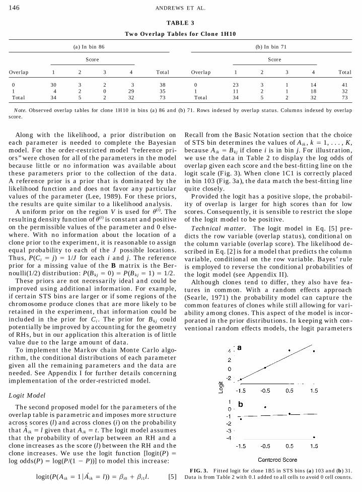
Along with the likelihood, a prior distribution on Recall from the Basic Notation section that the choiceof STS bin determines the values of Aik , k Å 1, . . . , K,each parameter is needed to complete the Bayesian

model. For the order-restricted model ‘‘reference pri- because Aik Å Bkj if clone i is in bin j. For illustration,we use the data in Table 2 to display the log odds ofors’’ were chosen for all of the parameters in the model

because little or no information was available about overlap given each score and the best-fitting line on thelogit scale (Fig. 3). When clone 1C1 is correctly placedthese parameters prior to the collection of the data.

A reference prior is a prior that is dominated by the in bin 103 (Fig. 3a), the data match the best-fitting linequite closely.likelihood function and does not favor any particular

values of the parameter (Lee, 1989). For these priors, Provided the logit has a positive slope, the probabil-ity of overlap is larger for high scores than for lowthe results are quite similar to a likelihood analysis.

A uniform prior on the region V is used for u(i). The scores. Consequently, it is sensible to restrict the slopeof the logit model to be positive.resulting density function of u(i) is constant and positive

on the permissible values of the parameter and 0 else- Technical matter. The logit model in Eq. [5] pre-where. With no information about the location of a dicts the row variable (overlap status), conditional onclone prior to the experiment, it is reasonable to assign the column variable (overlap score). The likelihood de-equal probability to each of the J possible locations. scribed in Eq. [2] is for a model that predicts the columnThus, P(Ci Å j) Å 1/J for each i and j. The reference variable, conditional on the row variable. Bayes’ ruleprior for a missing value of the B matrix is the Ber- is employed to reverse the conditional probabilities ofnoulli(1/2) distribution: P(Bkj Å 0) Å P(Bkj Å 1) Å 1/2. the logit model (see Appendix II).

These priors are not necessarily ideal and could be Although clones tend to differ, they also have fea-improved using additional information. For example, tures in common. With a random effects approachif certain STS bins are larger or if some regions of the (Searle, 1971) the probability model can capture thechromosome produce clones that are more likely to be common features of clones while still allowing for vari-retained in the experiment, that information could be ability among clones. This aspect of the model is incor-included in the prior for Ci . The prior for Bkj could porated in the prior distributions. In keeping with con-potentially be improved by accounting for the geometry ventional random effects models, the logit parametersof RHs, but in our application this alteration is of littlevalue due to the large amount of data.

To implement the Markov chain Monte Carlo algo-rithm, the conditional distributions of each parametergiven all the remaining parameters and the data areneeded. See Appendix I for further details concerningimplementation of the order-restricted model.

Logit Model

The second proposed model for the parameters of theoverlap table is parametric and imposes more structureacross scores (l) and across clones (i) on the probabilitythat Aik Å l given that Aik Å t. The logit model assumesthat the probability of overlap between an RH and aclone increases as the score (l) between the RH and theclone increases. We use the logit function [logit(P) Ålog odds(P) Å log(P/(1 0 P))] to model this increase:

FIG. 3. Fitted logit for clone 1B5 in STS bins (a) 103 and (b) 31.Data is from Table 2 with 0.1 added to all cells to avoid 0 cell counts.logit(P(Aik Å 1ÉAO ik Å l)) Å bi0 / bi1l. [5]

AID GENO 4652 / 6r2f$$$263 03-15-97 00:54:29 gnmal

STATISTICAL METHODS FOR BINNING CLONES 147

localized to bin 20 because the posterior probability,according to the logit model, for that bin is 0.71. Clone2E7 (Fig. 4b) is localized to bin 41 but with less confi-dence. A clone map is built by localizing each clone tothe STS bin with the maximum posterior probabilityfor that clone. Because the priors in our model are dom-inated by the likelihood, the maximum posterior proba-bility of clone location will not differ substantially froma maximum likelihood estimate.

Evaluating a Map

To evaluate the performance of each mappingmethod, we use the RPCI data of clone-by-clone com-parisons. Using PCR products from inter-Alu sites, theFIG. 4. Posterior distributions from logit model for four clones:RPCI data consist of hybridization probings of RPCI(a) 1A2, excellent; (b) 2E7, intermediate; (c) 7C5, poor; and (d) 15H3,YACs against a gridded YAC library to produce groupsambiguous.of proximate YACs. Of the YAC clones we analyze, onlya subset were assessed by RPCI. Because the map posi-for the I clones are a priori assumed to follow a bivari-tions of these YAC proximity groups are largely un-ate normal distribution with unknown mean g and un-known, they cannot be used to directly assess the map-known covariance matrix S,ping methods; however, they can provide an indirectassessment in conjunction with a statistical analysisbi Ç N2(g, S).based on maximum likelihood.

A key assumption of the maximum likelihood analy-This is a typical assumption for any random effectslogit analysis (Zeger and Karim, 1991). sis is that the elements of a RPCI cluster belong in the

same STS bin or nearby STS bins. Given this assump-The random effects logistic model is considerablymore complex than the order-restricted model, but tion, the principle behind the maximum likelihood

method is simple: if the mapping method is effective,some generalizations can be made about where themethod will place a clone based on the form of the the clusters it forms based on placing YACs in the same

or nearby bins should be very similar to the YAC clus-summary table. The observed logits (log(n(ij)1l /n(ij)

0l )) mustcorrespond roughly to a line that has a positive slope. ters formed by the RPCI hybridization experiments.

We wish to estimate this degree of similarity. We em-If multiple STS bins provide good fits to the data, thelogit model favors those bins with steeper logit slopes. ployed two likelihood methods to evaluate the degree

of similarity: the method described in Perlin et al.However, the random effects model forces a certainamount of commonality of logits for clones in their fa- (1995) and a refinement of that method. Because the

two methods produced essentially identical results, wevored placements. For instance, suppose that the ob-served logits (log(n(ij)

1l /n(ij)0l )) for STS bin j correspond report only the results using the Perlin et al. (1995)

method.quite closely to a line with a slope considerably greaterthan those observed for other clones. A random effectmodel is likely to favor STS bin j* over j if its observed CHROMOSOME 11 MAPlogits (log(n(ij=)

1l /n(ij=)0l )) fit reasonably closely to a line with

a slope similar to that found for other clones. One of the key features of our likelihood-based analy-To ensure that high scores are associated with over- sis is that it assigns to each clone a probability of mem-

lap and low scores with nonoverlap, the mean logit bership for each STS bin. Taken over all STS bins, theslope is constrained to be positive (g1 ú 0). Given that set of probabilities is called the posterior probabilitythere is no other a priori information on the value of distribution. These probability distributions, one forthe remaining parameters, we use standard reference each clone, determine in large part the probability ofprior distributions on the rest of the parameter space. correctly classifying a clone to its STS bin. AssumingFurther discussion of the model formulation, the prior the statistical modeling assumptions are approxi-distributions, the complete conditionals, the starting mately correct, these probabilities can be interpretedvalues, and other implementation details for the logit as the probability that the clone belongs in specific bins,model are included in Appendix II. given the data at hand. As an example we reproduce

these distributions for four clones (Fig. 4), estimatedObtaining a Map using the logit model, which represent results having

a range of classification properties: excellent, interme-To estimate the posterior probability that clone i be-longs in STS bin j, we use Markov chain Monte Carlo diate, poor, and ambiguous. Our level of confidence in

binning appropriately declines as the maximum proba-simulation. The STS bin with the maximum posteriorprobability is the best choice for the location of the bility decreases.

In general we take the bin with the maximum poste-clone. For example, clone 1A2 (Fig. 4a) is confidently

AID GENO 4652 / 6r2f$$$263 03-15-97 00:54:29 gnmal

ANDREWS ET AL.148

TABLE 4 within 5% of the maximum, there are 49, 52, and 359clones with near-ties for the logit, order-restricted andEstimated Performance of Three Mapping MethodsL2-min models, respectively. Thus the statistical meth-

Mapping methods ods yield more interpretable results in several ways:Number of they yield posterior probabilities of clone membership

clones mapped Logit Order-restricted L2-min to each STS bin; they are more accurate, in general;and they are precise, yielding few ties and near-ties for300 0.90 0.86 0.88clone location and overall a more refined location for400 0.86 0.83 0.85

500 0.86 0.81 0.80 each clone.600 0.82 0.80 0.74 We use the classification derived from the logit and700 0.80 0.76 0.72 order-restricted models to refine the chromosome 11800 0.76 0.71 0.69

map produced by Perlin et al. (1995). Rather than re-produce the entire map, we illustrate a small, continu-Note. Estimated performance of the three mapping methods. Val-

ues in the table are maximum likelihood estimates of the probability ous section of it, from STS bin 172 to STS bin 181. Thisof successfully mapping each member of a group of clones. section is selected because it contains the CRYA2 gene

(centered approximately at bin 177), and 13 of the YACclones are known to span the gene.rior probability of membership as the estimated loca-

tion for the clone. Thus these probabilities are critical. For the top 800 clones, all three mapping methodsagree on the bin location for the majority (63/100) ofTo construct a map for each method, we bin only the

800 clones that have the highest maximum posterior the clones mapped to this region by at least one of themethods (Table 5). In addition, most of the clones inprobabilities or L2-min scores (henceforth, the ‘‘top

800’’). The posterior probabilities corresponding to the this ‘‘agreement’’ table are mapped with high posteriorprobabilities. Of the 13 clones forming the CRYA2 con-top 800 clones are §0.1209 and §0.1606 for the logit

and order-restricted models, respectively; for the L2-TABLE 5min method, it is §0.3059. Notice that the cutoff value

for the logit model excludes the poorly mapped clone Map Agreement Tablein Fig. 4c from further consideration.

The top 800 clones differed somewhat by method. To Bin Clone (logit, order-restricted, L2-min)examine the mapping properties of clones with differ-

172 1E4 (96, 98, 79) 6B9 (88, 92, 79) 6E9 (65, 55, 63)ent maximum posterior probabilities or L2-min scores,11F6 (95, 88, 63) 12A1 (98, 73, 75) 12A3 (64, 31, 46)we first arranged the clones in descending order based 12B1 (99, 97, 65) 12C2 (47, 71, 48) 12C3 (16, 93, 39)

on their maximum posterior probability or L2-min 15A11 (99, 99, 95) 15E1 (93, 86, 72) 16A12 (82, 52, 84)score (i.e., largest to smallest value); then we subdi-

173 4A1 (84, 87, 50) 6C11 (96, 89, 83) 11A8 (35, 23, 38)vided the top 800 clones into groups, from the top 300 11G3 (36, 57, 38) 13G9 (71, 32, 57) 15A9 (50, 50, 85)to the top 800, by hundreds. 15A12 (85, 94, 57) 15G12 (99, 99, 95) 16G11 (94, 99, 89)

19G8 (99, 96, 68)We evaluate the performance of the binning methodsfor the top 800 clones by using the subdivisions just 174 2D6 (76, 58, 37) 6C10 (73, 92, 74) 8F7 (72, 82, 82)described and a maximum likelihood method described 12H9 (74, 54, 52) 13A10 (88, 84, 79) 14A7 (99, 98, 91)in Perlin et al. (1995). For any subdivision of the top

175 1G11 (68, 63, 66) 4A3 (67, 59, 44) 4A8 (97, 99, 99)300 to top 800 clones, it is apparent that the logit model 5B2 (75, 68, 60) 8A12 (96, 94, 83) 18E8 (70, 73, 83)performs better than either the order-restricted model 19C2 (96, 99, 97)or the L2-min method (Table 4). The comparison is

176more complex when the order-restricted model is com-177 2E5 (88, 94, 78) 3F3 (97, 99, 83) 4H7 (43, 50, 65)pared to the L2-min method. For the top 300 and 400

7D5 (58, 86, 71) 12A5 (39, 23, 35) 12A6 (90, 96, 93)clones mapped, the L2-min method yields better classi-14F9 (26, 00, 43) 15E3 (99, 99, 99) 15E4 (97, 90, 86)fication than the order-restricted model, but perfor- 17F11 (71, 68, 83) 17F12 (96, 96, 91) 17H4 (99, 99, 87)

mance is reversed thereafter. Apparently sensible clas- 18G8 (99, 98, 79) 19F7 (49, 48, 83)sification methods such as the L2-min perform quite

178 7C6 (63, 60, 57) 18B5 (39, 41, 84)well when the data are close to the idealized structure,179 2G7 (56, 36, 86) 11B9 (68, 62, 68) 12D1 (14, 00, 32)but to successfully position clones using noisier data

12E11 (76, 75, 83) 17C10 (45, 37, 63) 18F12 (17, 20, 46)requires more rigorous statistical models.In addition to predicting the appropriate bin more 180 14E10 (81, 84, 77)

frequently, the statistical models are also more defini- 181 7B2 (49, 44, 37) 7B4 (20, 12, 42) 7F1 (19, 31, 00)tive in their placement of the clones than the L2-min 12D3 (49, 43, 53) 12F11 (56, 73, 74)method. Both the logit and the order-restricted model

Note. After each bin are listed the clones that all three methodshave no ties and have fewer near-ties in the posteriormap to that bin. Also included are clones that are mapped by two ofprobability of clone membership to STS bins than thethe methods to the bin and not mapped at all by the third methodL2-min method does for its scoring method. Again con- (indicated by ‘‘00’’). After each identification tag is the posterior prob-

sidering the top 800 clones, there are 48 clones with ability or score (1100) for each method (logit, order-restricted, andL2-min).ties for the L2-min model. If we consider other peaks

AID GENO 4652 / 6r2f$$$264 03-15-97 00:54:29 gnmal

STATISTICAL METHODS FOR BINNING CLONES 149

TABLE 6 duce a final map. This map is not based on any formalanalysis, but simply on visual inspection of the data.Map Disagreement TableIn addition to the consensus map (Table 5), we bin

RPCI Logi Order-restricted L2-min 19 other clones to this region (Table 7). To bin theseadditional clones, we rely on evidence from the RPCI

1E2 192 (12) 172 (28) nm (00) data that these clones cluster with other clones already2G8 174 (18) 174 (22) 126 (49) mapped to the region with high probability (i.e., clones3B7 173 (84) 173 (72) 174 (85)

from Table 5), placing the clones at a consensus locality4F7 179 (35) 179 (26) 177 (56)4G9 173 (45) 173 (96) 174 (72) based on the results of the mapping methods. One of4H1 172 (57) 172 (96) 175 (65) the clones, 4F7, agrees well with the RPCI data both5D12 46 (12) nm (00) 174 (33) in bin 179 (where the statistical methods place it) and5G10 174 (39) 71 (40) 174 (43)

in bin 177 (where the L2-min method places it), and6A1 177 (30) 181 (29) 177 (42)thus it appears twice in Table 7. Of the 16 clones in6G12 174 (66) 174 (93) 126 (50)

8H7 172 (62) 172 (80) 174 (55) the ‘‘disagreement’’ table (Table 6) mapped to the same9D2 nm (00) 175 (16) nm (00) bin by the statistical methods, 8 could be confirmed by9F2 172 (33) 172 (37) 177 (32) the RPCI data. This result, which is a minimum esti-12A2 173 (42) 173 (35) 172 (63)

mate of performance due to the partial information12B3 nm (00) 172 (48) nm (00)available in the RPCI data, strongly suggests that us-12C1 179 (31) 173 (30) 179 (44)

12C5 nm (00) 172 (46) nm (00) ing the statistical methods alone is an excellent map-12E3 nm (00) 172 (20) 146 (44) ping strategy.12E6 nm (00) 173 (25) 131 (57) The entire map can be viewed and downloaded by12E10 179 (36) 179 (54) 178 (63)

anyone accessing our website (address under Acknowl-12F10 175 (43) 174 (43) 174 (61)12H10 181 (57) 181 (42) 182 (64) edgments). Because the entire probability distribution13H12 177 (50) 178 (50) 177 (88) for clone membership to STS bins is often helpful when14A1 177 (50) 178 (49) 177 (97) localizing clones, we also provide the entire posterior14A8 174 (44) 174 (29) 173 (64) distribution for the top 800 at the website. In addition,14F5 172 (50) 173 (50) 172 (84)

we provide the consensus map, again using the infor-15H6 181 (64) 181 (28) 23 (64)18A3 177 (43) 176 (50) 181 (77) mation obtained from the RPCI data.18A5 172 (29) 173 (25) 177 (49)18A12 172 (24) nm (00) 232 (47)

DISCUSSION18B1 179 (46) 179 (63) 178 (86)18B9 175 (16) 235 (29) 174 (58)18C6 179 (34) 20 (28) 20 (75) One approach to the problem of sequencing the hu-18C12 173 (38) 173 (38) 172 (51) man genome is to map clones to their original genomic18D11 172 (13) 172 (21) 134 (37) locations, then determine a minimum tiling path of19C10 174 (39) 175 (31) 177 (70)

clones, and finally sequence that subset of clones. Ide-19G12 179 (15) 26 (17) 179 (59)ally the clones used for this top-down strategy would

Note. The clones that are mapped to the region 172–181 by at be short DNA fragments such as BACs or PACs. As yet,least one of the three methods. Columns 2–4 indicate where each no top-down strategy has been developed in sufficientmethod maps the clone and with what posterior probability or score generality to sequence the genome.(1100). ‘‘00’’ indicates that the clone is not mapped by the method

An important tool available for sequencing the hu-(i.e., not in the top 800).man genome is a fairly dense STS framework map

tig, 12 map to the region. The 13th clone is not in theTABLE 7top 800 for the logit model and therefore is not consid-

ered. It is in the top 800 for the other two methods, but Map Supplementdoes not map to the region.

Bin CloneThe true locations for the remaining clones (37/100),which are mapped to the region by at least one of the

172 1E2, 2G3three methods, is somewhat ambiguous (Table 6). Not 173 3B7, 4G9, 12A2, 14F5only do the mapping methods exhibit some disagree- 174 2G8, 6G8

175 12F10, 19C10ment on bin membership for these clones, the posterior176probabilities or L2-min scores are frequently unimpres-177 4F7, 6A1sive. The statistical mapping methods agree in the178 13H12, 14A1

placement far more often (16/37) than either does with 179 4F7, 18B1, 18C6, 19G12the L2-min placements (7/37 for the logit model and 2/ 180 15H6

181 12H1037 for the order-restricted model).While a consolidated map could be based on the re-

Note. Additional clones placed in the region of STS bins 172–181sults of the statistical methods alone, we choose to use using information from RPCI clone/clone hybridization data. Thesethat information in conjunction with the L2-min clones cluster well with the unambiguously mapped clones in the

agreement table (Table 5).method and the RPCI clone/clone hybridizations to pro-

AID GENO 4652 / 6r2f$$$264 03-15-97 00:54:29 gnmal

ANDREWS ET AL.150

(Hudson et al., 1995). Because the map is evolving at clones to STS bins than either the order-restricteda rapid rate, a denser version should be available in model or the L2-min method (Table 4). When the order-the near future. While the map will undoubtedly be restricted method is compared to L2-min, the L2-minuseful for sequencing the genome, how it will be used method appears to perform better for ‘‘high-confidence’’remains to be seen. clones (i.e., the top 400 clones), but the performance is

Clearly the framework map could be used in conjunc- reversed for lower-confidence clones (Table 4).tion with STS content mapping (Green and Green, Much of this behavior can be explained by the con-1991) to localize the DNA fragments. Such an ap- gruity between the data and the assumptions imposedproach, however, would require an enormous number by the models. For instance, the logit model imposesof PCR experiments. Therefore it may not be the most the assumption that, when the clone is placed in theefficient strategy for localizing and choosing clones to correct STS bin, the probability that an STS and ansequence. RH overlap increases linearly on the logit scale with

One alternative strategy is to use IPM in conjunction increasing RH/YAC overlap score (for the same RH).with the framework map to localize the clones. The There is no rigorous molecular motivation for this as-IPM strategy combines noisy long-range data (RH/ sumption. However, the logit model frequently pro-clone hybridization data) with almost noise-free short- vides a good summary for data of this form (Agresti,range data (RH/STS overlap data) to infer, indirectly, 1990), and the assumption of increasing probability ofclone locations. This indirect approach has the notable RH/STS overlap with increasing RH/YAC overlap scorebenefit of significantly reducing the number of labora- certainly makes sense from the molecular perspective.tory experiments required to map clones relative to di- L2-min imposes a different linearity assumption,rect methods such as STS-content mapping. Thus IPM namely that the probability that an STS and an RHsolves the clone-mapping problem at lower cost. More- overlap increases linearly with increasing RH/YACover, by eliminating the need for direct clone and STS overlap score (Perlin et al., 1995). While this assump-comparisons, it enables clone mapping even when tion and that for the logit model may seem almost iden-clones and STSs do not overlap, as will often be the tical, it is well known that the error structure (constantcase for YAC clones mapped against relatively sparse variance) for the L2-min model is not optimal for theSTS maps and for small insert (bacterial) clones kind of data analyzed.mapped against even relatively dense STS maps. The order-restricted model imposes only a very weak

YACs are far larger than either BACs or PACs, which assumption about the form of the data. It is a nonpara-are more desirable substrates for sequencing. Nonethe- metric model, whereas the logit and L2-min models areless, in principle there is no reason why the IPM strat- parametric models (imposing linearity assumptions).egy cannot be effective for localizing smaller clones, Without an immense amount of data, parametric mod-although some redesign of the experimental methods els typically perform better than nonparametric modelsmay be required. In fact, recent research on whole- when the parametric model assumptions roughly con-genome RHs by Perlin (unpublished) suggests that the form to the true process generating the data. However,IPM strategy is implementable at this scale. as the disparity between assumptions and the process

Our results show that statistical methods can be tai- generating the data increase, the performance of thelored to the IPM top-down strategy, providing accurate nonparametric model is expected to improve. We sus-and interpretable results (in this instance) for clone bin- pect that this scenario explains the performance of L2-ning. Using these methods, we refine the chromosome min versus the order-restricted model: the assumption11 map (Tables 5, 6, and 7) first presented by Perlin et imposed by L2-min is adequate for high-confidenceal. (1995). Our analyses suggest that the improvement clones but is less adequate for lower-confidence clones.is substantial, not only in terms of the localizing the An important feature of the logit model is its randomclones (Table 4) but also in terms of the confidence with effects structure. This structure forces the slope fromwhich they are localized. Moreover, the availability of a particular 2 1 L table (e.g., Table 2) to shrink towardmaps based on different statistical models, together a common slope, that being the average slope over allwith supplemental information from RPCI, yields a such tables. Shrinkage in this setting is well known tohighly accurate clone map (Tables 5 and 7). increase the accuracy of the estimated slopes (Efron

While the binning of clones to local regions is an and Morris, 1973) and therefore should increase theimportant step in the process of building a minimal accuracy of the classification. In fact, when we com-tiling path of clones, it is obviously not a complete an- pared the random effects model to the standard maxi-swer. Nevertheless, by using the binning information mum likelihood logit model using the chromosome 11in conjunction with information on clone length and data, we found the classification performance of theclone overlap (Qin et al., 1996), it should be possible random effects model to be superior.to build such tiling paths very efficiently. Statistical It is unnecessary for a researcher to choose betweenmethods to address this problem is one focus of our

the logit and the order-restricted methods. While thecurrent genomics research.logit model outperforms the order-restricted model for

Statistical Methods the data we have analyzed (Table 4), these resultsspeak only to the average performance. The resultsBased on our analyses of the chromosome 11 data,

it appears that the logit model is better at assigning from the logit model are critically dependent on its lin-

AID GENO 4652 / 6r2f$$$264 03-15-97 00:54:29 gnmal

STATISTICAL METHODS FOR BINNING CLONES 151

earity assumption—which appears to hold generally, An obvious drawback to this binning method is thatit requires the STSs be ordered accurately on the chro-but may not be valid for a specific clone. Thus, for map-

ping clones to STS bins, it should be quite useful to mosome (i.e., STS j is adjacent to STS j / 1). Clearlythe bins make little sense when the ordering is inaccu-examine the results of both methods, particularly if the

methods localize clones to very different bins. In fact, rate. In fact, the ordering is unlikely to be perfect forthese or any other data available at this time (Lunettato produce the final map (Tables 5 and 6 and website),

we used information from all three methods and the and Boehnke, 1994). Nonetheless, this drawback maynot be as much of an impediment as it appears.Roswell Park clone/clone hybridization data.

Lange and Boehnke (1992) present a Bayesian modelto determine the order of STSs on a chromosome fromFuture DevelopmentsRH/STS overlap experiments. This model, possibly

In this report we have illustrated some statistical with some minor revisions, can be combined with themethods, in particular Bayesian hierarchical models, analyses we just outlined to form a more complexfor one step in the complex process of sequencing a Bayesian hierarchical model. Based on this more com-large genome. Theoretically, it should be possible to plex model, it should be possible to improve (iteratively)build a hierarchical model for the entire process. To do the binning of clones while also refining the order ofso, the kind of errors introduced at each level of the the STSs.process must be characterized and modeled (e.g., errorsin base-calling and errors in STS framework maps).

APPENDIX I: ORDER-RESTRICTED MODELThe resulting hierarchical model would undoubtedlyimprove the accuracy of any resulting sequence and A Markov chain Monte Carlo (MCMC) simulationprobably the speed by which the sequence is deter- iteratively samples from the conditional distribution ofmined. The model would be complex—perhaps too com- each parameter given the data as well as all the otherplex to analyze exactly—but approximations can be parameters. This conditional distribution is known asapplied to produce good solutions. the complete conditional distribution. For notational

An example of how more complex models can be built convenience we refer to the set of conditioning eventsfollows naturally from the methods we just developed. as ‘‘the rest.’’ The complete conditionals are derivedIn this brief example, we describe how to build upon from the likelihood and the prior distributions usingthe hierarchical Bayes binning methods to refine the Bayes’ rule. Because all prior distributions for the or-assignment of clones to bins while also refining the der-restricted model are constant over the parameterorder of STSs in an STS framework map (see Mukho- space, the complete conditionals are proportional to thepadhyay et al. [1994] for a preliminary approach to this likelihood on that region. Specifically, the complete con-problem). ditional distributions for the order-restricted model are

We assumed early in our analyses that each cloneshould be classified to exactly one STS bin. If two STSsare close together, it is likely that a clone in that region P(Ci Å j*Érest) Å ∏1

tÅ0 ∏LlÅ1 [u(i)

tl ]n(ij*)tl

(JjÅ1 ∏1

tÅ0 ∏LlÅ1 [u(i)

tl ]n(ij)tl

,will overlap both of them rather than just one. Withour techniques the clone is likely to fit well into both j* √ {1, . . . , J};STS bins. For STSs separated by greater distances, theclones will most likely fall between these STSs. In fact,

P(Bkj Å t*Érest) Å∏{i:CiÅj} u

(i)t*AO ik

(1tÅ0 ∏{i:CiÅj} u

(i)tAO ik

, t* √ {0, 1};the clones might not be close to either STS. These ob-servations suggest another means of creating STS bins.

andDefine bins based on the region between adjacent pairsof STS bins rather than on the region surrounding indi-vidual STSs. f(u(i)*Érest) Å ∏1

tÅ0 ∏LlÅ1 [u(i)*]

n(ij)

tl

*V ∏1tÅ0 ∏L

lÅ1 [u(i)]n(ij)

tl du(i), u(i)* √ V,

Define B by

where V is as defined by Eq. [3] under Statistical Analy-ses. The parameter space for each Ci and missing BkjBkj Å

1 if a fragment of RH k and STS j overlap,

1 if a fragment of RH k and STS j / 1 overlap,

0 otherwise.is discrete so the denominators of the complete condi-tionals are found by direct computation. However, toavoid computing the many-dimensional integral in thedenominator of the complete conditional of u(i), we em-When we applied this alternative model to the chromo-

some 11 data, the performance of the new model was ploy a Metropolis–Hastings step (Tierney, 1994; Has-tings, 1970).mixed. Some clones that had been previously mapped

to two STS-centered bins, each with moderate posterior The starting values of the parameters come from ran-dom sampling from prior distributions and maximumprobability, were now mapped with high posterior

probability to a single inter-STS bin. However, many likelihood estimates. First we obtain starting values forthe missing values of the B matrix by random samplingclones that previously had been mapped very well were

no longer mapped well. from a Bernoulli(1/2) distribution. Next approximate

AID GENO 4652 / 6r2f$$$264 03-15-97 00:54:29 gnmal

ANDREWS ET AL.152

maximum likelihood estimates for u(i) are found for pi1 , . . . , piL01) that yields identical probability distri-butions for A (Roeder et al., 1996). This is not a hin-each clone i in each bin j. The estimate found is close

to the maximum likelihood estimate and is guaranteed drance here because interest is only on the likelihoodof the tables themselves, not the particular parametersto be in the region V. To compute the starting value,that define the tables. Nevertheless, due to the lackfor l Å 1, . . . , L and t Å 0, 1, let htl Å (L

l=Ålu(i)tl= , and

of identifiability, the model must be constrained forestimate them bycomputational stability.

To make the model fully identifiable, only one of thehP 0l Å minS(L

l=Åln(ij )0l=

n(j )0/

,(L

l=Åln(ij )/l=

K D L parameters bi0 , pi1 , . . . , piL01 needs to be specified foreach i. However, because A has significant informationabout the values of pi , each component of pi is estimatedandfrom the observed marginal values from table A. Thesevalues are then assumed to be fixed (as opposed to

hP 1l Å maxS(Ll=Åln

(ij )1l=

n(j )1/

,(L

l=Åln(ij )/l=

K D . random quantities) for the analysis [see item (e) below].This assumption, while not strictly accurate, leads tostable performance and enhanced speed of convergenceLast, u(i)

tl Å hP tl 0 hP tl/1 , where hP tL/1 Å 0. Each clone’sfor the MCMC algorithm. Furthermore, it does not no-initial placement (Ci) is the bin where its approximateticeably affect the final conclusions drawn from themaximum likelihood occurs.data.The sampling order is each u(i), the missing values of

the B matrix, and then C. Results are based on theImplementation Detailslast 8000 iterations of a 10,000-iteration simulation.

The logit model described in this appendix is repa-APPENDIX II: LOGIT MODEL rametrized slightly, relative to that in the body of the

paper, so that the sampling distributions are easier toBayes’ Rule evaluate. Specifically, the vectors bi are rewritten g /

bi . Then Eq. [5] becomes [after recentering the valuesThe logit model as described under Statistical Analy-in A to sl Å 0(L 0 1)/2, . . . , (L 0 1)/2 from l Å 1, . . . ,ses is not completely specified because the conditionalL)]probability in Eq. [5] must be reversed via Bayes’ rule.

To employ Bayes’ rule, the marginal column and rowlogit{P(Aik Å 1ÉAO ik Å l)} Å g0 / bi0 / (g1 / bi1)sl .probabilities must be specified. These are pil Å P(Aik Å

l) and qit Å P(Aik Å t), respectively. Note that qit is aThe distribution of the bi , which can be inferred fromknown quantity determined by the row margins, whichthe distribution of the bi , is bivariate normalare fixed for each STS bin. Now use Bayes’ rule to

rewrite u(i)tl in terms of the parameters in this model:

bi Ç N2(0, S).u(i)

tl Å P(AO ik Å lÉAik Å t)Listed below are the remaining variables in the logit

model and their prior distributions including the twoÅ P(Aik Å tÉAO ik Å l)P(AO ik Å l)P(Aik Å t) table marginals that we estimated from their observed

values.Å [g(l, bi)]t[1 0 g(l, bi)]10tpil

qit, [6]

(a) Ci Ç Uniform on {1, . . . , J}.(b) Bkj Ç Bernoulli(1/2) for missing values in B.(c) g } 1 on R1R/. The mean slope parameter mustwhere

be positive.(d) S } ÉSÉ03/2 on the space of all positive definite 2

g(l, bi) Å P(Aik Å 1ÉAO ik Å l) Å exp(bi0 / bi1l)1 / exp(bi0 / bi1l)

1 2 matrices.(e) pil Å (n(i)

/l / 1)/(K / L), the posterior mode if theprior distribution for pi were flat.

is derived from Eq. [5]. The full likelihood function can (f) qit Å n(j)t//K, where Ci Å j.

then be obtained directly by substitution of Eq. [6] intoEq. [2]. All of the priors were chosen to be reference priors,

hence the likelihood dominates the prior and no partic-Because the row margins are fixed for a given bin-ning C, the likelihood for this dataset is of the same ular values are favored a priori. The prior distributions

for Ci and Bkj are also ‘‘proper,’’ meaning the sum overform as the product of I case–control studies (Breslowand Day, 1980) times the product of I multinomials. It all possible outcomes is 1. By contrast, the standard

choice of reference priors for g and S are ‘‘improper,’’is well known that the logit model is not fully identifi-able under case–control sampling (i.e., more than one meaning that the integral over all possible values is

infinite.set of parameters yields the same maximum likeli-hood). This implies that there is a set of values of (bi , The specified hierarchical structure and the prior

AID GENO 4652 / 6r2f$$$265 03-15-97 00:54:29 gnmal

STATISTICAL METHODS FOR BINNING CLONES 153

distributions result in the following complete condition- data and good starting values, this region of the param-eter space will not be visited. The chromosome 11 data-als where u(i)

tl (g, bi) is defined in Eq. [6]:set is large enough and the starting values found frommaximum likelihood methods are good enough to avoid

P(Ci Å j*Érest) Å ∏1tÅ0 ∏L

lÅ1 [u(i)tl (g, bi )]n

(ij*)tl

(JjÅ1 ∏1

tÅ0 ∏LlÅ1 [u(i)

tl (g, bi )]n(ij)tl

, the trouble area. Under these conditions we obtain (inpractice) a proper posterior.

j* √ {1, . . . , J };

ACKNOWLEDGMENTSP(Bkj Å t*Érest) Å

∏{i:CiÅj} [u(i)t*AO ik(g, bi )]

(1tÅ0 ∏{i:CiÅj} [u(i)

tAO ik(g, bi )]

,This research was supported in part by a doctoral fellowship from

AT&T (C.A.), NSF Grants DMS9496219 (K.R.) and DMS9508427t* √ {0, 1}; (B.D. and K.R.), and NIH Grants HG00348 (B.D.) and HG00856

(M.P.). The address of the web site that contains the map of chromo-some 11 and C programs to implement these methods is www.stat.f (g*Érest) Å ∏I

iÅ1 ∏1tÅ0 ∏L

lÅ1 [u(i)tl (g*, bi )]n

(ij)tl

*R1R/

∏IiÅ1 ∏1

tÅ0 ∏LlÅ1 [u(i)

tl (g, bi )]n(ij)tl dg

,cmu.edu/Çroeder/map/map.html.

REFERENCESg* √ R 1 R/; S01*Érest Ç Wishart2(I, (∑I

iÅ1

bib*i )01);

Agresti, A. (1990). ‘‘Categorical Data Analysis,’’ Wiley, New York.Aho, A. V., Hopcroft, J. E., and Ullman, J. D. (1983). ‘‘Data Struc-and

tures and Algorithms,’’ Addison-Wesley, Reading, MA.Bellanne-Chantelot, C., Lacroix, B., Ougen, P., Billault, A., Beaufils,

S., Bertrand, S., Georges, S., Glibert, F., Gros, I., Lucotte, G., Sus-ini, L., Codani, J.-J., Gesnouin, P., Pook, S., Vaysseix, G., Lu-Kuo,J., Ried, T., Ward, D., Chumakov, I., Le Paslier, D., Barillot, E.,and Cohen, D. (1992). Mapping the whole genome by fingerprinting

f (b*i Érest) Å

expS0 12

b**i (01b*i D∏1tÅ0

1 ∏LlÅ1 [u(i)

tl (g, b*i )]n(ij)tl

*R2

expS0 12

b*i(01biD∏1

tÅ0

1 ∏LlÅ1 [u(i)

tl (g, bi )]n(ij)tl dbi

, b*i √ R2. yeast artificial chromosomes. Cell 70: 1059–1068.Berger, J. O. (1985). ‘‘Statistical Decision Theory and Bayesian Anal-

ysis,’’ 2nd ed., Springer–Verlag, New York.Breslow, N. E., and Day, N. E. (1980). ‘‘Statistical Methods in Cancer

Research,’’ Vol. 1, ‘‘The Analysis of Case–Control Studies,’’ IARC,Lyon.

The exact distribution of (01 is known and can be Cox, D. R., Burmeister, M., Price, E. R., Kim, S., and Myers, R. M.(1990). Radiation hybrid mapping: A somatic cell genetic methodsampled directly. The parameter spaces for each Ci andfor constructing high-resolution maps of mammalian chromo-missing Bkj are discrete so the constants of proportion-somes. Science 250: 245–250.ality are found by summation. The distributions of g

Cox, D. R., Green, E. D., Lander, E. S., Cohen, D., and Myers, R. M.and bi are continuous so it is more feasible to use a(1994). Assessing mapping progress in the human genome project.Metropolis–Hastings step than to evaluate the two- Science 265: 2031–2032.

dimensional integrals in the denominators. Efron, B., and Morris, C. (1973). Stein’s estimation rule and its com-Again, starting values of the parameters are ob- petitors—An empirical Bayes approach. J. Am. Stat. Assoc. 68:

tained by random sampling from prior distributions 117–130.and maximum likelihood estimates. First we obtain Gelfand, A. E., and Smith, A. F. M. (1990). Sampling-based ap-

proaches to calculating marginal densities. J. Am. Stat. Assoc. 85:starting values for the missing values of the B matrix398–409.by random sampling from a Bernoulli(1/2) distribution.

Geyer, C. (1989). Practical Markov chain Monte Carlo. Stat. Sci. 4:For each i, J estimates of bi are obtained by fitting a473–482.logit model with clone i placed in each STS bin using

Green, E. D., and Green, P. (1991). Sequence-tagged site (STS) con-maximum likelihood methods. Clone i is placed in thetent mapping of human chromosomes: Theoretical considerationsbin where its maximum likelihood logit score occurs. and early experiences. PCR Methods Appl. 1: 77–90.

The fitted value of bi that corresponds with the binning Hastings, W. K. (1970). Monte Carlo sampling methods using Mar-that maximizes the likelihood is retained. The starting kov chains and their applications. Biometrika 57: 97–109.value for g is the mean of the fitted bi’s and finally bi Hudson, T. J., Stein, L., Gerety, S. S., Ma, J., Castle, A. B., Silva, J.,Å bi 0 g. With starting values for all parameters but ( Slonim, D. K., Baptista, R., Kruglyak, L., Xu, S.-H., et al. (1995).

An STS-based map of the human genome. Science 270: 1945–1954.specified, the initial value for ( can be sampled directlyJames, M. R., Richard, C. W., III, Schott, J.-J., Yousry, C., Clark, K.,from its complete conditional.

Bell, J., Hazan, J., Dubay, C., Vignal, A., Agrapart, M., et al. (1994).The sampling order is (, the missing values of the BA radiation hybrid map of 506 STS markers spanning human chro-matrix, C, g, and then bi . Results are based on the last mosome 11. Nature Genet. 8: 70–76.

8000 iterations of a 10,000-iteration simulation.Lange, K., and Boehnke, M. (1992). Bayesian methods and optimal

The marginal posterior distribution of ( is improper experimental design for gene mapping by radiation hybrids. Ann.for this hierarchical model. The density function in- Hum. Genet. 56: 119–144.creases without bound as É(É r 0. This region can Lee, P. M. (1989). ‘‘Bayesian Statistics: An Introduction,’’ Arnold,

London.cause poor performance in a MCMC chain if the param-eter becomes trapped here. However, with sufficient Lunetta, K., and Boehnke, M. (1994). Multipoint radiation hybrid

AID GENO 4652 / 6r2f$$$265 03-15-97 00:54:29 gnmal

ANDREWS ET AL.154

mapping: Comparisons of methods, sample size requirements, and B. H., Bric, E., Housman, D. E., Evans, G. A., and Shows, T. B.(1996). A high-resolution physical map of human chromosome 11.optimal study characteristics. Genomics 21: 92–103.Proc. Natl. Acad. Sci. USA 93: 3149–3154.Monaco, A. P., Lam, V. M. S., Zehetner, G., Lennon, G. G., Douglas,

Qin, S., Zhang, J., Isaacs, C. M., Nagafuchi, S., Jani, S. S., Abel, K. J.,C., Nizetic, D., Goodfellow, P. N., and Lehrach, H. (1991). MappingHiggins, M. J., Nowak, N. J., and Shows, T. B. (1993). A chromo-irradiation hybrids to cosmid and yeast artificial chromosome li-some 11 YAC library. Genomics 16: 580–585.braries by direct hybridization of Alu-PCR products. Nucleic Acids

Richard, C., III, Boehnke, M., Berg, D., Lichy, J., Meeker, T., Myers,Res. 19: 3315–3318.R., and Cox, D. (1993). A radiation hybrid map of the distal shortMukhopadhyay, N., Gorin, M. B., and Perlin, M. W. (1994). Orderingarm of human chromosome 11 containing the Beckwith–Weide-STSs via YAC hybridizations to radiation hybrids using innermann and associated embryonal tumor disease loci. Am. J. Hum.product mapping. Am. J. Hum. Genet. 55(Suppl.): A266.Genet. 52: 915–921.

Nelson, D. L., Ledbetter, S. A., Corbo, L., Victoria, M. F., Ramirez- Richard, C., III, Withers, D., Meeker, T., Maurer, S., Evans, G., My-Solis, R., Webster, T. D., Ledbetter, D. H., and Caskey, C. T. (1989). ers, R., and Cox, D. (1991). A radiation hybrid map of the proximalAlu polymerase chain reaction: A method for rapid isolation of long arm of human chromosome 11 containing the multiple endo-human-specific sequences from complex DNA sources. Proc. Natl. crine neoplasia type 1 (MEN-1) and bcl-1 disease loci. Am. J. Hum.Acad. Sci. USA 86: 6686–6690. Genet. 49: 1189–1196.Nowak, N., Qin, S., Zhang, J., Sait, S., Higgins, M., Cheng, Y., Li, Roeder, K. R., Carroll, R. J., and Lindsay, B. G. (1996). A semipara-

L., Munroe, D., Evans, G., Housman, D., and Shows, T. (1994). metric mixture approach to case–control studies with errors inGenerating a physical map of chromosome 11. Am. J. Hum. Genet. covariables. J. Am. Stat. Assoc. 91: 722–732.55(Suppl.): A267. [Abstract] Searle, S. R. (1971). ‘‘Linear Models,’’ Wiley, New York.

Perlin, M. W., and Chakravarti, A. (1993). Efficient construction of Smith, A. F. M., and Roberts, G. O. (1993). Bayesian computation viahigh-resolution physical maps from yeast artificial chromosomes the Gibbs sampler and related Markov chain Monte Carlo meth-using radiation hybrids: Inner product mapping. Genomics 18: ods. J. R. Stat. Soc. B 55: 3–24.283–289. Tanner, M. A., and Wong, W. H. (1987). The calculation of posterior

Perlin, M. W., Duggan, D. J., Davis, K., Farr, J. E., Findler, R. B., distributions by data augmentation. J. Am. Stat. Assoc. 82: 528–Higgins, M. J., Nowak, N. J., Evans, G. A., Qin, S., Zhang, J., 540.Shows, T. B., James, M. R., and Richard, C. W., III (1995). Rapid Tierney, L. (1994). Markov chains for exploring posterior distribu-construction of integrated maps using inner product mapping: YAC tions (with discussion). Ann. Stat. 22: 1701–1762.coverage of human chromosome 11. Genomics 28: 315–327. Zeger, S., and Karim, M. R. (1991). Generalized linear model with

random effects: A Gibbs sampling approach. J. Am. Stat. Assoc.Qin, S., Nowak, N. J., Zhang, J., Sait, S. N. J., Mayers, P., Higgins,M. J., Cheng, Y., Li, L., Munroe, D. M., Gerhard, D. S., Weber, 86: 79–86.

AID GENO 4652 / 6r2f$$$266 03-15-97 00:54:29 gnmal