Binomial Autoregressive Processes with Density

Dependent Thinning

Christian H. Weiß∗ and Philip K. Pollett†

October 2, 2013

Abstract

We present an elaboration of the usual binomial AR(1) process on {0, 1, . . . , N} that

allows the thinning probabilities to depend on the current state n only through the

“density” n/N , a natural assumption in many real contexts. We derive some basic

properties of the model and explore approaches to parameter estimation. Some special

cases are considered that allow for over- and underdispersion, as well as positive and

negative autocorrelation. We derive a law of large numbers and a central limit theorem,

which provide useful large–N approximations for various quantities of interest.

Key words: binomial AR(1) model; binomial INARCH(1) model; stationarity; nor-

mal approximation; overdispersion and underdispersion; metapopulation models; pa-

rameter estimation.

∗Department of Mathematics and Statistics, Helmut Schmidt University, Postfach 700822, D-22008 Ham-

burg, Germany. weissc@hsu-hh.de†Department of Mathematics, University of Queensland, QLD 4072, Australia. pkp@maths.uq.edu.au

1

1 Introduction

In recent times there has been considerable interest in time series of count data with a

fixed finite range {0, 1, . . . , N}. Applications include the monitoring of computer pools

(with N workstations) (Weiß, 2009; Weiß & Kim, 2013a), of infections (with N individuals)

(Daley & Gani, 1999, Section 4.4), of metapopulations (with N patches) (Buckley & Pollett,

2009, 2010a,b; Weiß & Pollett, 2012), and of transactions in the stock market (with N

listed companies) (Weiß & Kim, 2013b). A popular model is the binomial AR(1) process,

proposed by McKenzie (1985) as an integer-valued counterpart to the standard Gaussian

AR(1) process. It is defined using the binomial thinning operation introduced by Steutel &

van Harn (1979): α ◦ x :=∑x

i=1 yi, where the yi are i.i.d. Bernoulli variables with success

probability α, independent of the count-data random variable x (given x, α◦x ∼ Bin(x, α)).

If α and β are suitable thinning probabilities, the process (nt, t = 0, 1, . . . ), taking values in

{0, . . . , N}, defined by the recursion

nt = α ◦ nt−1 + β ◦ (N − nt−1) (t ≥ 1),

where all thinnings are performed independently of one another, and where the thinnings at

time t are independent of (ns, s < t), is called a binomial AR(1) process. (A similar model,

which instead uses hypergeometric thinning, was developed by Al-Osh & Alzaid (1991).)

Properties of the binomial AR(1) process are now well understood. It is an ergodic

Markov chain with a Bin(N, π) stationary distribution, where π = β/(1− r) and r = α− β,

and its autocorrelation function is given by ρ(k) = rk (k ≥ 0) (analogous to the Gaussian

AR(1) process). Its h-step regression properties were explored in Weiß & Pollett (2012),

where it was also shown that, for large N , the process can be approximated by a Gaussian

2

AR(1) process. Closed-form expressions for the joint moments and cumulants were derived

in Weiß & Kim (2013a), and questions concerning parameter estimation were addressed in

Cui & Lund (2010); Weiß & Kim (2013a,b); Weiß & Pollett (2012).

A significant limitation of the binomial AR(1) model is that the thinning probabilities at

time t do not depend on the process up to that time. For example, in the epidemic context, if

nt represents the number of infectives and N −nt the number susceptibles in a population of

size N (Daley & Gani, 1999, Section 4.4), or, in the metapopulation context, if nt represents

the number of occupied habitat patches and N − nt the number unoccupied in an N -patch

population (Buckley & Pollett, 2010a), it is natural to allow α and/or β to depend on nt,

reflecting the (internal) infection-recovery or colonization-extinction mechanisms. Such a

state-dependence of the parameters is also plausible in an economic context, where it may

arise, for example, through the interaction of supply and demand; see also our analysis of

securities data in Section 4.2.

Our purpose here is to extend the binomial AR(1) model to allow this kind of state

dependence, thus increasing its applicability. As we shall see, if the thinning probabilities

are allowed to depend on nt only through the “density” nt/N (for example, the proportion of

infectives or proportion of occupied patches), then many of the properties of the basic model

can be extended without difficulty. Similar state-dependent thinning has been considered

previously in the context of the INAR(1) model by McKenzie (1985): the FINAR(1) model

(Triebsch, 2008) and the SETINAR(2, 1) model (Monteiro et al., 2012).

A formal definition of a density-dependent binomial AR(1) process is given in Section 2.

Here we derive some of its basic properties and indicate approaches to parameter estimation.

In Section 3 we a derive a law of large numbers and a central limit theorem, thus providing

3

useful large–N approximations for various quantities of interest. Then we focus on several

special cases within the family of density-dependent binomial AR(1) models: in Section 4 we

study a case that is convenient for modelling over- and underdispersion (as well as positive

and negative autocorrelation), and in Section 5 we give special attention to the case where

α (only) is constant. Our conclusions are summarized in Section 6.

2 Density-dependent Binomial AR(1) Processes

Following the approach of Buckley & Pollett (2010a), we extend the definition of the binomial

AR(1) model to allow the model parameters to be density dependent.

Definition 2.1. Let π : [0; 1] → (0; 1) and r : [0; 1] → (0; 1), so that the functions β(y) :=

π(y)(1 − r(y)

)and α(y) := β(y) + r(y), defined for y ∈ [0; 1], also have range (0; 1). Fix

N ≥ 1 and write πt := π(nt−1/N), rt := r(nt−1/N), αt := α(nt−1/N) and βt := β(nt−1/N),

so that the thinning probabilities at time t satisfy βt := πt (1 − rt) and αt := βt + rt. The

process (nt, t ≥ 0), taking values in {0, . . . , N} and defined by the recursion

nt = αt ◦ nt−1 + βt ◦ (N − nt−1) (t ≥ 1),

where the thinnings at time t are performed independently of one another and of (ns, s < t),

is called a density-dependent binomial AR(1) process.

A process thus defined is a time-homogeneous finite-state Markov chain with transition

probabilities

P (k|l) := Pr(nt = k | nt−1 = l) =∑min {k,l}

m=max {0,k+l−N}(lm

) (N−lk−m

) (α(l/N)

)m(1− α(l/N)

)l−m (β(l/N)

)k−m(1− β(l/N)

)N−l+m−k(> 0),

(1)

4

from which the following regression properties are readily obtained:

E(nt | nt−1) = rt nt−1 +N βt,

Var(nt | nt−1) = rt(1− rt) (1− 2πt)nt−1 +N βt(1− βt).

(2)

For details, see Appendix A.1.

2.1 Unique Stationary Solution

Notice that the transition matrix P = (P (k|l)k,l=0,...,N) is primitive, implying that the process

is ergodic with uniquely determined stationary distribution. Whilst in some special cases

a closed-form expression can be obtain for this distribution, it is not available in general,

nor even are there closed-form expressions for its mean and variance. However, given a

particular parametric form, these quantities can always be determined numerically. Let

p =(P (0), . . . , P (N)

)⊤denote the stationary probability vector, where P (k) = Pr(nt = k).

Then p is obtained from the equation Pp = p, and it can be used, for example, to evaluate

stationary moments of nt. For second-order moments with time-lag h, as required to evaluate

the autocorrelation function, one uses Pr(nt = k, nt−h = l), being the entries of Ph diag(p).

Furthermore, large–N approximations are available; in Section 3.3, we obtain closed-form

approximations for stationary mean, variance and autocorrelation function, the quality of

which improve as N becomes large.

2.2 Approaches to Parameter Estimation

In any particular application the functions α and β will depend on a vector of model pa-

rameters θ, which lie in some open subset Θ of Rs. Using formula (1), the conditional

5

log-likelihood of observing n1, . . . , nT , given n0, is

ℓ(θ) =T∑t=1

lnPθ(nt|nt−1).

Maximum likelihood (ML) estimates for θ are obtained numerically by maximizing ℓ(θ). We

can prove, in the stationary case, existence, consistency and asymptotic normality of the

conditional ML estimator θML of θ using Theorems 2.1 and 2.2 of Billingsley (1961). It

suffices to check Condition 5.1 of Billingsley (1961): for all θ ∈ Θ,

(i) Pθ(k|l) is three times continuously differentiable with respect to θ, and

(ii) the (N + 1)2 × s matrix with entries ∂∂θu

Pθ(k|l) has rank s.

This approach is exemplified below in Sections 4 and 5, where we consider some three-

parameter models (s = 3).

Remark 2.2.1 (Moment Estimation). For the above-mentioned numerical procedure, it is

natural to use method of moments (MM) estimates for the initial values. For some types of

stationary density-dependent binomial AR(1) model (like the one described in Section 4.1),

it is possible to find closed-form expressions for moments, autocorrelation function, et cetera.

In such cases, moment relations are used to obtain parameter estimates based on empirically

determined moments. If no closed-form expressions are available (as is the case for the model

considered in Section 5), we recommend using an approximate method of moments based on

the large–N moment approximations derived in Section 3.3.

6

3 Large–N Approximations

Let (nt, t ≥ 0) be a density-dependent binomial AR(1) process and define (XN

t , t ≥ 0) by

XN

t = nt/N . By varying N we obtain a family of Markov chains that is density-dependent

in the sense of (Buckley & Pollett, 2010a, Section 3). In particular, it follows from (2) that

E(XN

t |XN

t−1) = f(XN

t−1), where

f(x) = α(x)x+ β(x)(1− x) = r(x)x+ β(x), (3)

and N Var(XN

t |XN

t−1) = v(XN

t−1), where

v(x) = α(x)(1− α(x))x+ β(x)(1− β(x))(1− x). (4)

3.1 A Law of Large Numbers

Since 0 ≤ XN

t ≤ 1, we may apply Theorem 1 of Buckley & Pollett (2010a) to obtain the

following law of large numbers.

Theorem 3.1.1. Suppose that α and β are continuous and bounded. If X0P→ x0 (a constant)

as N → ∞, then XN

tP→ xt for all t ≥ 1, where (xt) is determined by xt+1 = f(xt) (t ≥ 0).

Thus for large N our binomial AR(1) process can be approximated by a deterministic

process (xt), the form of which is determined by the thinning probabilities. Since f is

not necessarily a linear function, (xt) can potentially exhibit the full range of long-term

behaviour, including limit cycles and even chaos. However, since f(x) = x if and only if(1− r(x)

)x = β(x) = π(x)

(1− r(x)

), we can see that x∗ is a fixed point of f if and only if

(a) x∗ is a fixed point of π, or

7

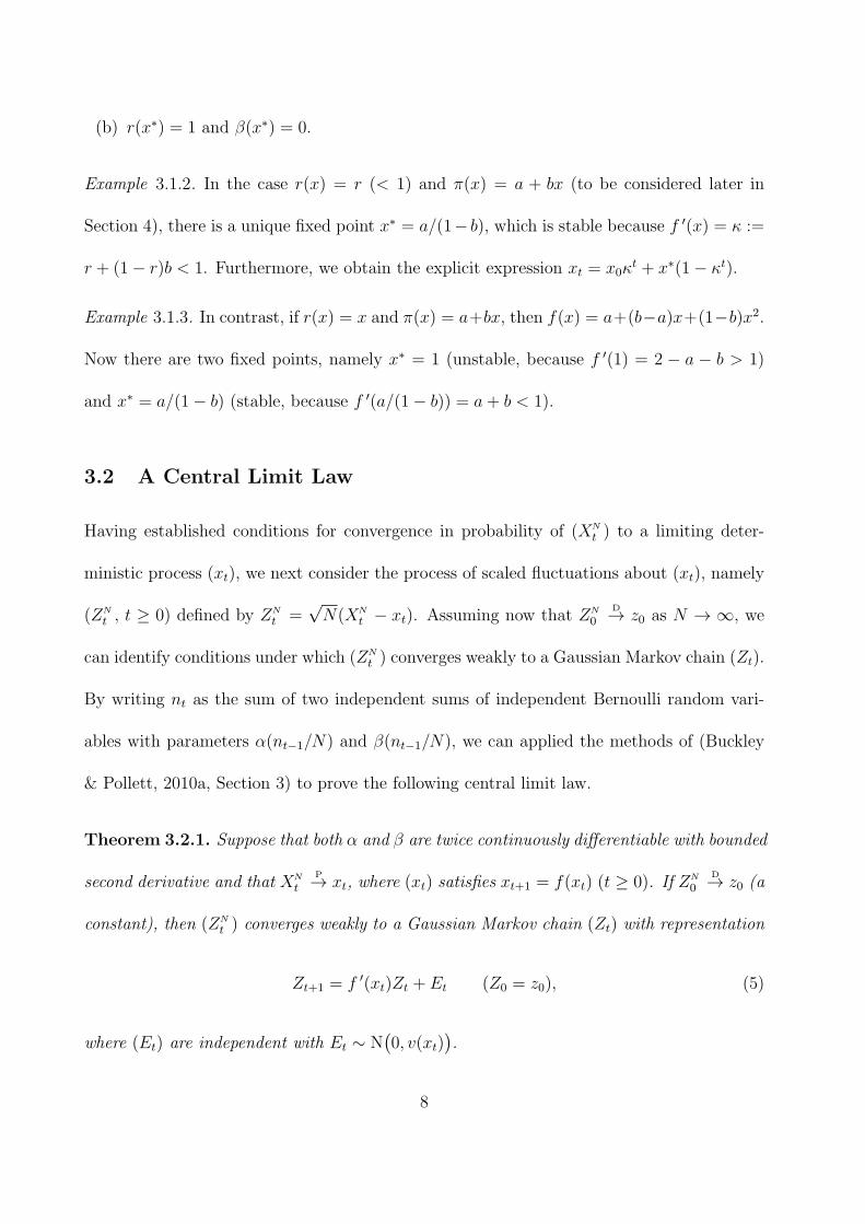
(b) r(x∗) = 1 and β(x∗) = 0.

Example 3.1.2. In the case r(x) = r (< 1) and π(x) = a + bx (to be considered later in

Section 4), there is a unique fixed point x∗ = a/(1− b), which is stable because f ′(x) = κ :=

r + (1− r)b < 1. Furthermore, we obtain the explicit expression xt = x0κt + x∗(1− κt).

Example 3.1.3. In contrast, if r(x) = x and π(x) = a+bx, then f(x) = a+(b−a)x+(1−b)x2.

Now there are two fixed points, namely x∗ = 1 (unstable, because f ′(1) = 2 − a − b > 1)

and x∗ = a/(1− b) (stable, because f ′(a/(1− b)) = a+ b < 1).

3.2 A Central Limit Law

Having established conditions for convergence in probability of (XN

t ) to a limiting deter-

ministic process (xt), we next consider the process of scaled fluctuations about (xt), namely

(ZN

t , t ≥ 0) defined by ZN

t =√N(XN

t − xt). Assuming now that ZN

0D→ z0 as N → ∞, we

can identify conditions under which (ZN

t ) converges weakly to a Gaussian Markov chain (Zt).

By writing nt as the sum of two independent sums of independent Bernoulli random vari-

ables with parameters α(nt−1/N) and β(nt−1/N), we can applied the methods of (Buckley

& Pollett, 2010a, Section 3) to prove the following central limit law.

Theorem 3.2.1. Suppose that both α and β are twice continuously differentiable with bounded

second derivative and that XN

tP→ xt, where (xt) satisfies xt+1 = f(xt) (t ≥ 0). If ZN

0D→ z0 (a

constant), then (ZN

t ) converges weakly to a Gaussian Markov chain (Zt) with representation

Zt+1 = f ′(xt)Zt + Et (Z0 = z0), (5)

where (Et) are independent with Et ∼ N(0, v(xt)

).

8

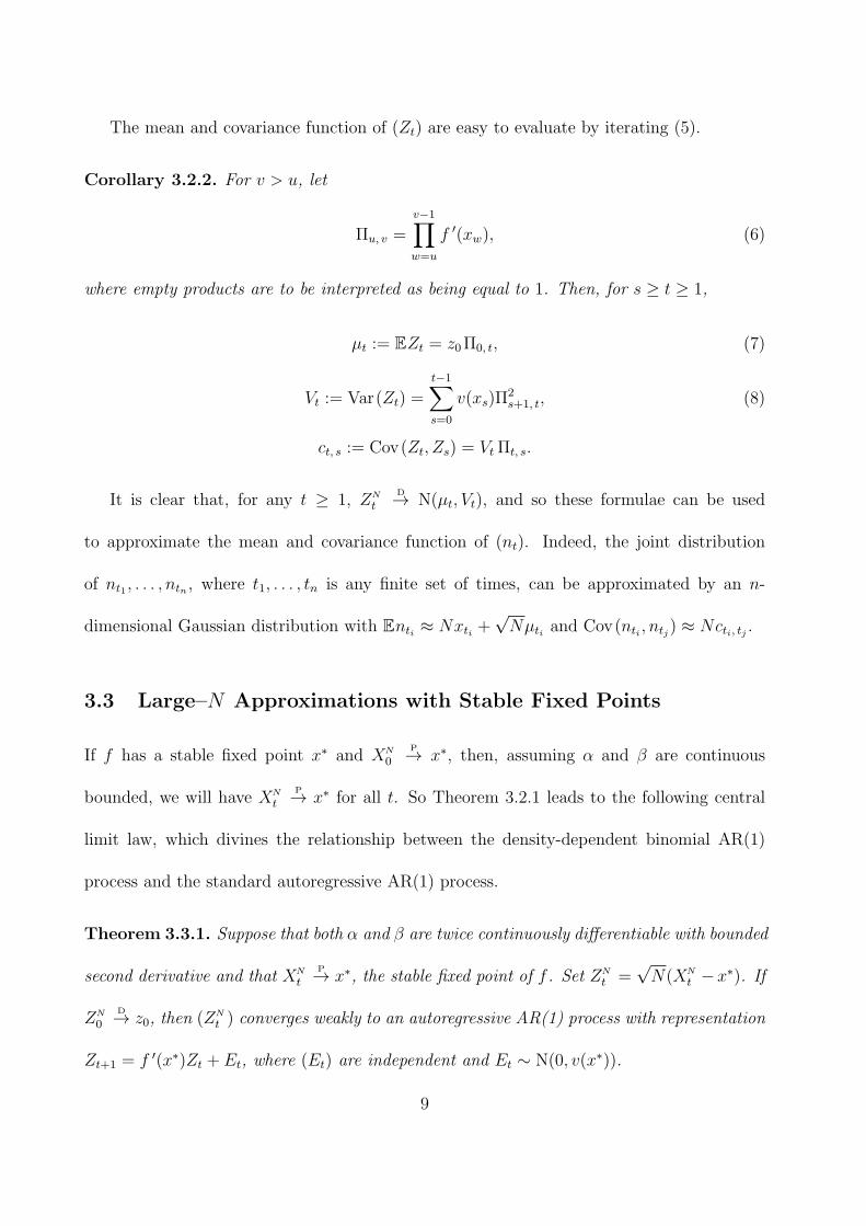
The mean and covariance function of (Zt) are easy to evaluate by iterating (5).

Corollary 3.2.2. For v > u, let

Πu, v =v−1∏w=u

f ′(xw), (6)

where empty products are to be interpreted as being equal to 1. Then, for s ≥ t ≥ 1,

µt := EZt = z0Π0, t, (7)

Vt := Var(Zt) =t−1∑s=0

v(xs)Π2s+1, t, (8)

ct, s := Cov(Zt, Zs) = Vt Πt, s.

It is clear that, for any t ≥ 1, ZN

tD→ N(µt, Vt), and so these formulae can be used

to approximate the mean and covariance function of (nt). Indeed, the joint distribution

of nt1 , . . . , ntn , where t1, . . . , tn is any finite set of times, can be approximated by an n-

dimensional Gaussian distribution with Enti ≈ Nxti +√Nµti and Cov(nti , ntj) ≈ Ncti, tj .

3.3 Large–N Approximations with Stable Fixed Points

If f has a stable fixed point x∗ and XN

0P→ x∗, then, assuming α and β are continuous

bounded, we will have XN

tP→ x∗ for all t. So Theorem 3.2.1 leads to the following central

limit law, which divines the relationship between the density-dependent binomial AR(1)

process and the standard autoregressive AR(1) process.

Theorem 3.3.1. Suppose that both α and β are twice continuously differentiable with bounded

second derivative and that XN

tP→ x∗, the stable fixed point of f . Set ZN

t =√N(XN

t −x∗). If

ZN

0D→ z0, then (ZN

t ) converges weakly to an autoregressive AR(1) process with representation

Zt+1 = f ′(x∗)Zt + Et, where (Et) are independent and Et ∼ N(0, v(x∗)).

9

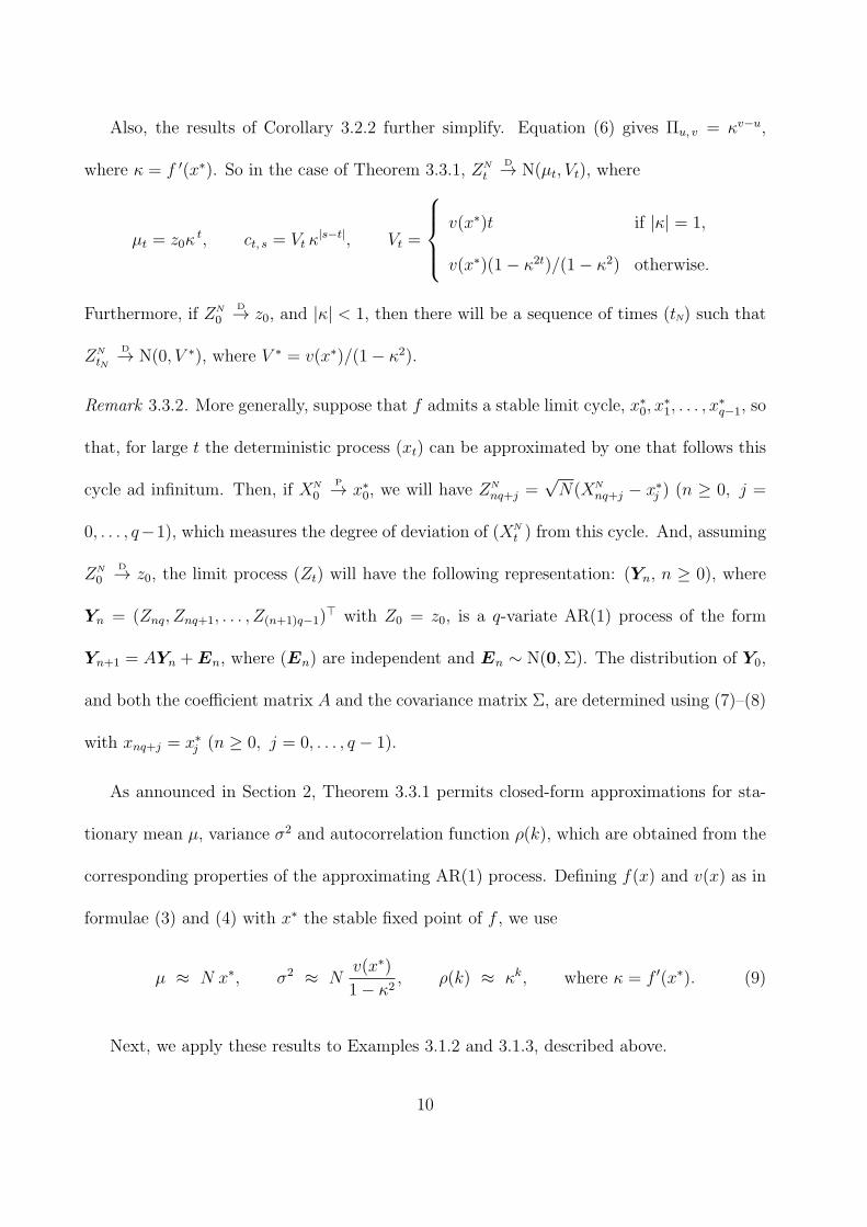
Also, the results of Corollary 3.2.2 further simplify. Equation (6) gives Πu, v = κv−u,

where κ = f ′(x∗). So in the case of Theorem 3.3.1, ZN

tD→ N(µt, Vt), where

µt = z0κt, ct, s = Vt κ

|s−t|, Vt =

v(x∗)t if |κ| = 1,

v(x∗)(1− κ2t)/(1− κ2) otherwise.

Furthermore, if ZN

0D→ z0, and |κ| < 1, then there will be a sequence of times (tN) such that

ZN

tN

D→ N(0, V ∗), where V ∗ = v(x∗)/(1− κ2).

Remark 3.3.2. More generally, suppose that f admits a stable limit cycle, x∗0, x

∗1, . . . , x

∗q−1, so

that, for large t the deterministic process (xt) can be approximated by one that follows this

cycle ad infinitum. Then, if XN

0P→ x∗

0, we will have ZN

nq+j =√N(XN

nq+j − x∗j ) (n ≥ 0, j =

0, . . . , q−1), which measures the degree of deviation of (XN

t ) from this cycle. And, assuming

ZN

0D→ z0, the limit process (Zt) will have the following representation: (Yn, n ≥ 0), where

Yn = (Znq, Znq+1, . . . , Z(n+1)q−1)⊤ with Z0 = z0, is a q-variate AR(1) process of the form

Yn+1 = AYn +En, where (En) are independent and En ∼ N(0,Σ). The distribution of Y0,

and both the coefficient matrix A and the covariance matrix Σ, are determined using (7)–(8)

with xnq+j = x∗j (n ≥ 0, j = 0, . . . , q − 1).

As announced in Section 2, Theorem 3.3.1 permits closed-form approximations for sta-

tionary mean µ, variance σ2 and autocorrelation function ρ(k), which are obtained from the

corresponding properties of the approximating AR(1) process. Defining f(x) and v(x) as in

formulae (3) and (4) with x∗ the stable fixed point of f , we use

µ ≈ N x∗, σ2 ≈ Nv(x∗)

1− κ2, ρ(k) ≈ κk, where κ = f ′(x∗). (9)

Next, we apply these results to Examples 3.1.2 and 3.1.3, described above.

10

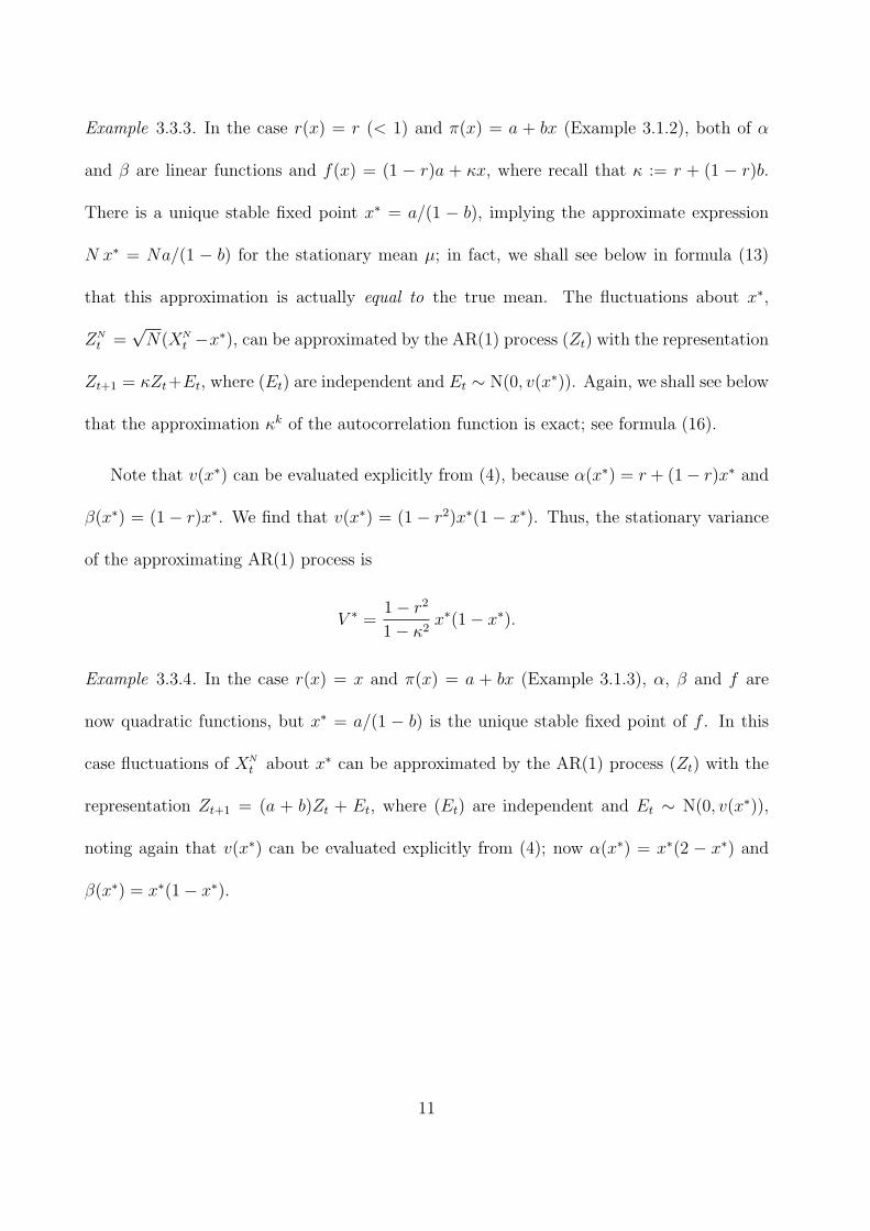
Example 3.3.3. In the case r(x) = r (< 1) and π(x) = a + bx (Example 3.1.2), both of α

and β are linear functions and f(x) = (1 − r)a + κx, where recall that κ := r + (1 − r)b.

There is a unique stable fixed point x∗ = a/(1 − b), implying the approximate expression

N x∗ = Na/(1 − b) for the stationary mean µ; in fact, we shall see below in formula (13)

that this approximation is actually equal to the true mean. The fluctuations about x∗,

ZN

t =√N(XN

t −x∗), can be approximated by the AR(1) process (Zt) with the representation

Zt+1 = κZt+Et, where (Et) are independent and Et ∼ N(0, v(x∗)). Again, we shall see below

that the approximation κk of the autocorrelation function is exact; see formula (16).

Note that v(x∗) can be evaluated explicitly from (4), because α(x∗) = r + (1− r)x∗ and

β(x∗) = (1 − r)x∗. We find that v(x∗) = (1 − r2)x∗(1 − x∗). Thus, the stationary variance

of the approximating AR(1) process is

V ∗ =1− r2

1− κ2x∗(1− x∗).

Example 3.3.4. In the case r(x) = x and π(x) = a + bx (Example 3.1.3), α, β and f are

now quadratic functions, but x∗ = a/(1 − b) is the unique stable fixed point of f . In this

case fluctuations of XN

t about x∗ can be approximated by the AR(1) process (Zt) with the

representation Zt+1 = (a + b)Zt + Et, where (Et) are independent and Et ∼ N(0, v(x∗)),

noting again that v(x∗) can be evaluated explicitly from (4); now α(x∗) = x∗(2 − x∗) and

β(x∗) = x∗(1− x∗).

11

4 Special Case: A Model for Binomial Overdispersion

or Underdispersion

For the Poisson distribution, the mean and variance are the same, a property commonly

referred to as equidispersion. An analogous fixed relation between the mean and the variance

also holds for the binomial distribution, and this might be expressed by using the so-called

binomial index of dispersion. For a random variable with finite support {0, . . . , N} and with

a certain mean µ and variance σ2, the binomial index of dispersion (as a function of N , µ

and σ2) is defined as

Id :=Nσ2

µ(N − µ)∈ (0;∞). (10)

In the case of a Bin(N, π)-distributed random variable, we have Id = 1 for any π ∈ (0; 1).

For this reason, finite-range count data random variables satisfying Id > 1 are said to

show overdispersion with respect to the binomial distribution (sometimes extra-binomial

variation), while underdispersion refers to the case Id < 1.

In this section, we study a special density-dependent binomial AR(1) model, where r(y) =

r, a constant, and π is a linear function. Notice then that α and β are also linear functions.

We shall see that the stationary case has very attractive features for real applications, because

we will be able to deal with both over- and underdispersion (in the above sense), as well as

positive and negative autocorrelation. Furthermore, this new model encapsulates a binomial

counterpart of the so-called INARCH(1) model; see Section 4.3 for details.

12

4.1 Definition and Stochastic Properties

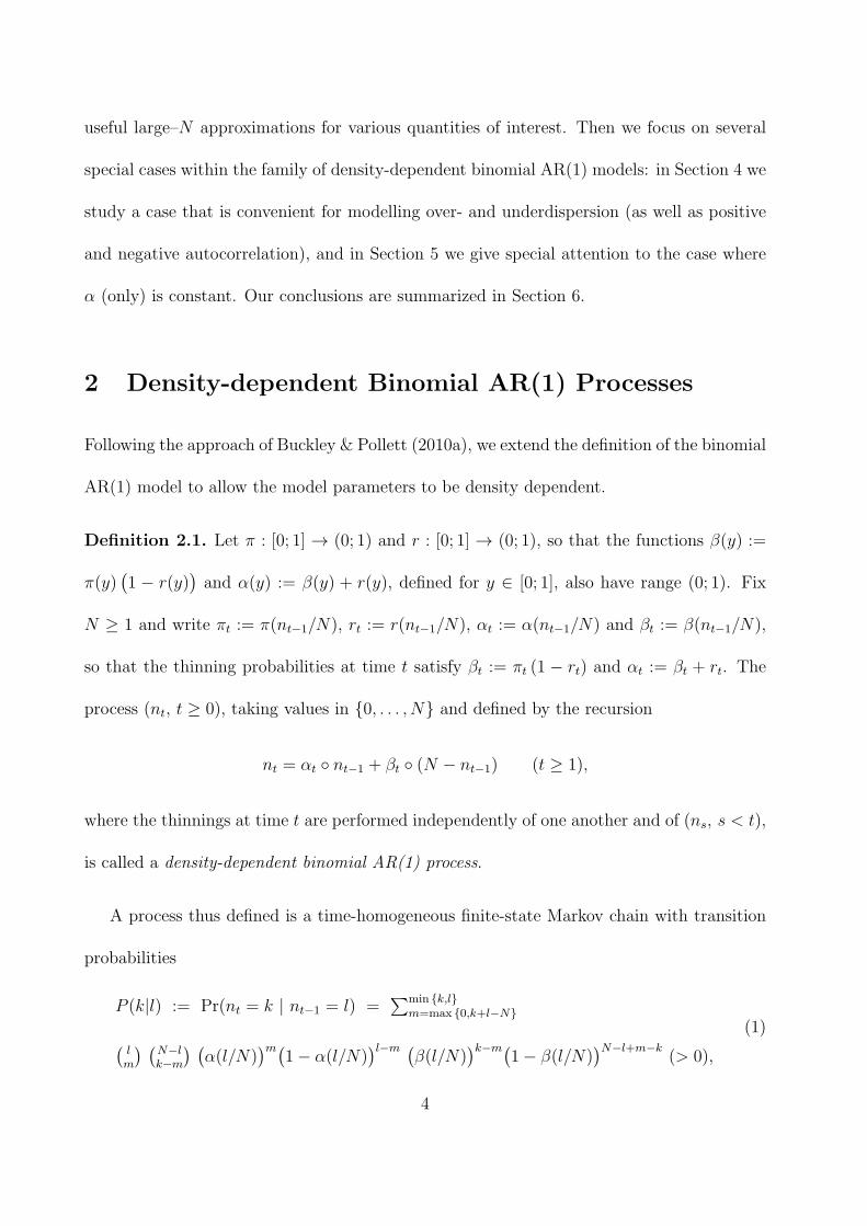
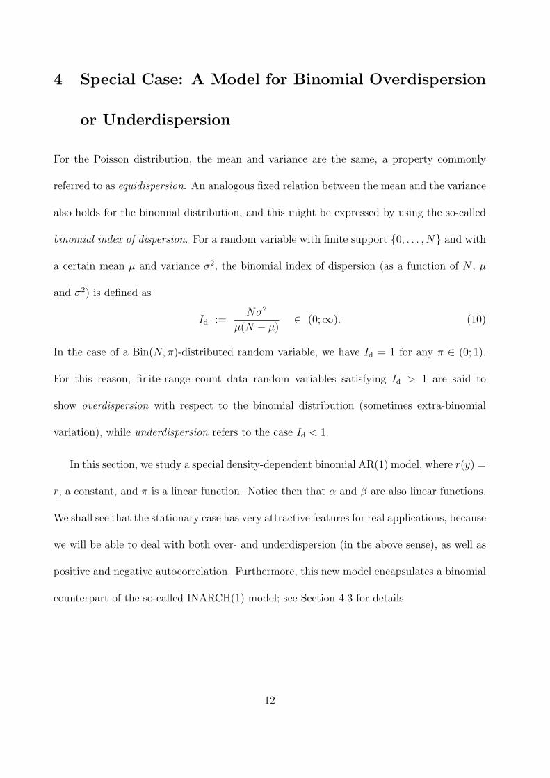
Suppose that π(y) = a+ by, where a, a+ b ∈ (0; 1). This entails π(y) ∈ (0; 1), but allows b to

also be negative (see Figure 1 (a)). If b > 0, then π increases with y (corresponding to the

upper triangle in Figure 1 (a)), while π decreases with increasing y if b < 0 (corresponding

to the lower triangle in Figure 1 (a)). b = 0 corresponds to density independence.

Notice that the thinning probabilities βt and αt from Definition 2.1 are also linear func-

tions that depend on the density nt/N through

βt = (1− r) (a+ b nt/N), αt = (1− r) (a+ b nt/N) + r.

So, depending on the sign of b, these probabilities increase or decrease with increasing density.

In a metapopulation context as mentioned in Section 1, for instance, we would conclude that

the occupation of patches becomes more attractive (b > 0) or less attractive (b < 0) if the

occupation rate is already large. In an economic context, b < 0 could reflect the interaction

of supply and demand.

Theorem 4.1.1. Let (nt, t ≥ 0) be a density-dependent binomial AR(1) process with r(y) =

r ∈ (0; 1), a constant, and π(y) = a+ by, where a, a+ b ∈ (0; 1). Then, for k = 1, 2, . . . , t,

E(nt | nt−k) =(r + (1− r)b

)knt−k +

Na

1− b

(1−

(r + (1− r)b

)k), (11)

in particular

E(nt | nt−1) =(r + (1− r)b

)nt−1 +N(1− r)a,

and

Var(nt | nt−1) = N(1− r)a(1− (1− r)a

)− b(1−r)

N

(2r + b(1− r)

)n2t−1

+ (1− r)((1− 2a)(b+ r) + 2abr

)nt−1.

(12)

13

(a)

1

3

2

31

a

-1

-0.5

0.5

1b

0

PossibleRange of b

(b)

1

3

2

31Ρ

-1

-0.5

0.5

1b

0

Underdispersion

Overdispersion

Over-dispersion

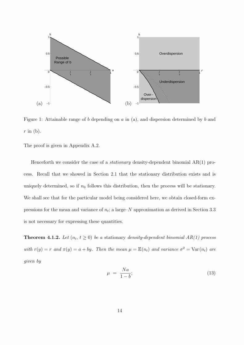
Figure 1: Attainable range of b depending on a in (a), and dispersion determined by b and

r in (b).

The proof is given in Appendix A.2.

Henceforth we consider the case of a stationary density-dependent binomial AR(1) pro-

cess. Recall that we showed in Section 2.1 that the stationary distribution exists and is

uniquely determined, so if n0 follows this distribution, then the process will be stationary.

We shall see that for the particular model being considered here, we obtain closed-form ex-

pressions for the mean and variance of nt; a large–N approximation as derived in Section 3.3

is not necessary for expressing these quantities.

Theorem 4.1.2. Let (nt, t ≥ 0) be a stationary density-dependent binomial AR(1) process

with r(y) = r and π(y) = a+ by. Then the mean µ = E(nt) and variance σ2 = Var(nt) are

given by

µ =Na

1− b; (13)

14

σ2 =1− r2

1− r2

N− (1− 1

N)(r + (1− r)b

)2 µ(1− µ

N)

=1 + r

1 + r − 2(1− 1N)rb− (1− 1

N)(1− r)b2

µ(1− µ

N).

(14)

The proof is given in Appendix A.2. Note that µ(1−µ/N) is the usual binomial variance. So,

the first factor in (14) is just the actual value of the binomial index of dispersion Id from (10)

and, hence, a measure of the deviation of the true distribution from a binomial distribution.

Remembering the large–N approximation from Example 3.3.3, where κ = r + (1 − r)b, we

note that

Id(N, b, r) =1− r2

1− r2

N− (1− 1

N)κ2

→ 1− r2

1− κ2(as N → ∞),

in accordance with the expression for V ∗.

For N > 1, we have

Id = Id(N, b, r)

>

=

<

1 iff b(2r + (1− r)b

) >

=

<

0,

that is, we have over-/equi-/underdispersion with respect to the binomial distribution ac-

cording to the following rule:

N = 1 or b = −2r1−r

or b = 0 ⇒ equidispersion,

N > 1 and b < −2r1−r

or b > 0 ⇒ overdispersion,

N > 1 and −2r1−r

< b < 0 ⇒ underdispersion.

(15)

If r > 13, then −2r

1−r< −1, that is, b < −2r

1−ris not possible in this case. So for r > 1

3and b < 0,

we always observe underdispersion. This is illustrated in Figure 1 (b).

15

Remark 4.1.3. If we take the partial derivative ∂∂b

Id(N, b, r) and equate it to 0 (see Ap-

pendix A.2), we see that for N > 1 the index of dispersion is minimal in b when b = −r1−r

(the dashed line in Figure 1 (b)) and increases above or below this value. So the strongest

underdispersion for given N and r is

Id(N, −r1−r

, r) =1− r2

1− r2

N

≥ 1− r2.

On the other hand,

limb→1 Id(N, b, r) =1− r2

1− r2

N− (1− 1

N)

= N,

limb→−1 Id(N, b, r) =1− r2

1− r2

N− (1− 1

N)(1− 2r)2

= N1 + r

1− 3r + 4Nr≤ N,

that is, the maximum possible overdispersion is below N ; see also the discussion in Hagmark

(2009). Note, however, that values of b close to ±1 severely restrict the choice of a according

to Figure 1 (a).

Finally, let us investigate the serial dependence structure. As shown in Appendix A.2,

the autocorrelation function is given by

ρ(k) =(r + (1− r)b

)k, (16)

analogous to the Gaussian AR(1) model. Since r ≥ 0, we obtain negative autocorrelations

(for odd k) iff b < −r1−r

, the latter being again the dashed line in Figure 1 (b). So dispersion

behaviour plus the sign of ρ(1) determine to which of the four regions in Figure 1 (b) the

pair (r, b) belongs.

16

4.2 Parameter Estimation and a Real-Data Example

As already discussed in Section 2.2, to prove existence, consistency and asymptotic normality

of the conditional ML estimator, we may check the conditions (i) and (ii) listed above in

Section 2.2. In the present case, α and β are polynomials in the three model parameters.

Hence, so is Pθ(k|l), and therefore differentiable up to any order. To verify (ii), we consider

the Jacobian ofPθ(0|0)

Pθ(0|1)

Pθ(1|1)

=

(1− β(0)

)N(1− α( 1

N)) (

1− β( 1N))N−1

(N − 1)(1− α( 1

N))β( 1

N)(1− β( 1

N))N−2

+ α( 1N)(1− β( 1

N))N−1

,

(17)

where θ = (a, b, r)⊤, α(y) = r + (1− r)(a+ by) and β(y) = (1− r)(a+ by). Its determinant

is obtained (after tedious computations) as

(N − 1) r(1− r)2(1− a(1− r)

)N−1 (1− (1− r)(a+ b/N)

)2(N−2).

Provided N > 1, this determinant is not equal to 0, implying that the Jacobian of (17) has

full rank of s = 3, which, in turn, implies that (ii) is satisfied.

Concerning the MM approach outlined in Remark 2.2.1, we note that the three model pa-

rameters a, b, r are determined through the relations (13) for the mean, (14) for the variance,

and (16) for the first-order autocorrelation.

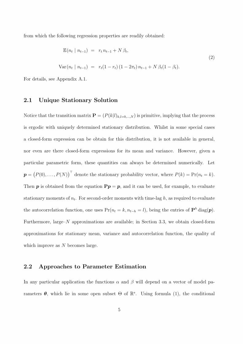
Example 4.2.1 (Securities Counts). We consider the count-data time series presented in

Section 4 of Weiß & Kim (2013b), being the number of different securities companies (among

N = 22 such companies) traded in the Korea stock market per 5-minute period on 8th

February 2011, during trading from 09:00 to 14:50 (see Figure 2). Each of the 70 counts can

17

10 20 30 40 50 60 70

5

10

15

20

Figure 2: Plot of the securities counts discussed in Example 4.2.1.

take a value between 0 and 22. The sample mean and variance are n ≈ 9.529 and s2 ≈ 4.253,

respectively. Analyzing the empirical (partial) autocorrelations, a first-order autoregressive

dependence structure is apparent for the securities counts.

As shown by Weiß & Kim (2013b), these data are well described by the standard binomial

AR(1) model. But, since the empirical index of dispersion Id = s2/(n(1 − n/N)

)≈ 0.787

indicates a slight degree of binomial underdispersion, one may ask if the data might be even

better described by the density-dependent binomial AR(1) model of Section 4.1. We first

computed moment estimates for the parameters a, b, r of this model. Substituting n ≈ 9.529,

s2 ≈ 4.253 and ρ(1) ≈ 0.402 in equations (13), (14) and (16), respectively, we obtain the

estimates

aMM ≈ 0.630, bMM ≈ −0.454, rMM ≈ 0.588.

These values were used to initialize the numerical procedure for computing the conditional

ML estimates (we used R’s nlm); the relevant results are summarized in Table 1. The ML

estimate for b is negative, so if many of the securities companies are traded, the probabili-

ties for trading activity become reduced. The ML-fitted density-dependent binomial AR(1)

model has a dispersion index of about 0.728 and, hence, describes the empirical level of

about 0.787 rather well. It also has a slightly lower value for Akaike’s information criterion

(AIC) than the usual binomial AR(1) model. But it performs worse in terms of the Bayesian

18

Table 1: Conditional ML estimates (together with the estimated standard errors in paren-theses) for the securities counts discussed in Example 4.2.1.

πML rML AIC BICBin. AR(1) 0.428 0.510 283.8 288.3

(0.022) (0.090)

aML bML rML AIC BICD.-D. Bin. AR(1) 0.693 –0.619 0.630 283.6 290.3

(0.198) (0.458) (0.083)

information criterion (BIC), and the estimate for b (the parameter that controls the den-

sity dependence) is not significantly different from 0. Both of these observations might be

due to the small sample size of 70.1 So, although the fitted density-dependent binomial

AR(1) model is able to describe the empirically observed underdispersion, the more sparsely

parameterized binomial AR(1) model seems adequate for the given count data time series.

4.3 Boundary Case r → 0: The Binomial INARCH(1) Model

The family of INGARCH(p, q) models constitutes an integer-valued counterpart to the usual

generalized autoregressive conditional heteroscedastic models (Ferland et al., 2006). The

model order (p, q)=(1, 0) leads to the INARCH(1) model, which gives a homogeneous Markov

chain. Most commonly, this model is defined using a conditional Poisson distribution, but

also versions with different types of count data distribution (always with a strictly infinite

range) have been considered in the literature. The popular Poisson INARCH(1) model

assumes that the process (zt) has the property that the current observation zt, given the

past zt−1, zt−2, . . ., stems from a conditional Poisson distribution with a mean being linear

1Note: Reparametrizing b = −a · d such that a, d, r ∈ (0; 1), the estimate for d (≈ 0.893) is significantly

different from 0 (s.e. ≈ 0.409).

19

in zt−1. The unconditional distribution of zt then shows overdispersion with respect to the

Poisson distribution. See Weiß (2010) for a survey of the INARCH(1) model.

Let us consider the density-dependent binomial AR(1) models with r(y) = r ∈ (0; 1), a

constant, and π(y) = a + by, where a, a + b ∈ (0; 1). In the boundary case r → 0, we have

α(y) = β(y) = π(y), and so the recursion of Definition 2.1 becomes

ntD= Bin

(N, π(nt−1/N)

)= Bin

(N, a+ b nt−1/N

)(t ≥ 1), (18)

in that the conditional distribution of nt given the past observations is a binomial distri-

bution with (conditional) success probability a + b nt−1/N . Motivated by the analogy to

the aforementioned (Poisson) INARCH(1) model, we shall refer to the model (18) as the

binomial INARCH(1) model.

The stationary mean of the binomial INARCH(1) model (18) is given by formula (13),

while formula (14) for the variance (taking r → 0) simplifies to

σ2 =µ(1− µ

N)

1− (1− 1N)b2

, that is, Id = Id(N, b, 0) =1

1− (1− 1N)b2

∈ [1;N). (19)

Consequently, only overdispersion is possible in this case, in accordance with rule (15) and

analogous to the case of the Poisson INARCH(1) model. Also, formula (16) simplifies to

ρ(k) = bk. Note that ρ(k) might also take negative values, which is in contrast to the case

of the Poisson INARCH(1) model. Another difference to the Poisson INARCH(1) model is

the fact that the conditional variance is not a linear but a quadratic function in nt−1:

E(nt | nt−1) = b nt−1 + N a,

Var(nt | nt−1) = N a (1− a) − b2

Nn2t−1 + (1− 2a) b nt−1.

(20)

20

10 20 30 40 50

5

10

15

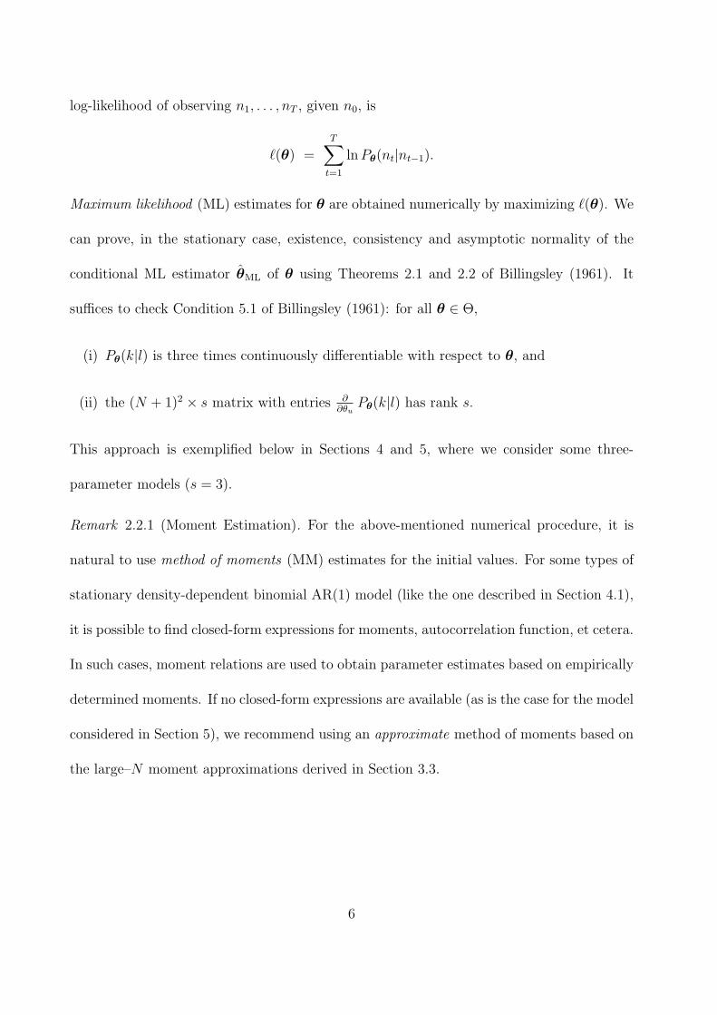
Figure 3: Plot of the infection counts discussed in Example 4.3.1, together with 1-step-ahead

forecasts (median and 95% interval).

Example 4.3.1 (Infection Counts). The online data base “SurvStat”, maintained by the

Robert Koch-Institut (RKI, 2013), provides a large source of epidemic data. Among others,

it offers weekly data about new cases of diverse infections in Germany that have been reported

to the RKI via local and state health departments. In the following, we use these data to

obtain condensed information about the regional spread of an infection with time. But,

instead of referring to the 16 federal states in Germany (which are very heterogeneous in

terms of population), we use the classification according to the N = 38 districts as defined

by the SurvStat data base.

For illustrative purposes, let us now concentrate on one specific infection, namely infec-

tions by the hantavirus in the year 2011 with its T = 52 weeks. So each count nt represents

the number of districts with a new case of hantavirus infection in week t. The observed

counts vary between 0 and 11; a plot of the data is shown in Figure 3. The empirical mean

and variance are given by n ≈ 4.173 and s2 ≈ 7.793, respectively. So the resulting value

Id ≈ 2.098 of the index of dispersion points to a considerable degree of overdispersion. An

inspection of the empirical (partial) autocorrelation function indicates use of an autoregres-

sive model for the data; in particular, we have ρ(1) ≈ 0.634. Using this information, we are

able to compute the moment estimates for the usual binomial AR(1) model, for the density-

21

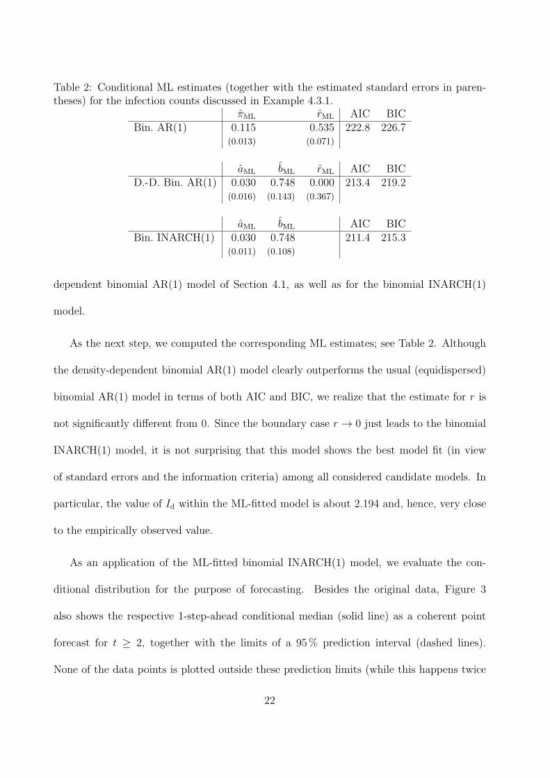
Table 2: Conditional ML estimates (together with the estimated standard errors in paren-theses) for the infection counts discussed in Example 4.3.1.

πML rML AIC BICBin. AR(1) 0.115 0.535 222.8 226.7

(0.013) (0.071)

aML bML rML AIC BICD.-D. Bin. AR(1) 0.030 0.748 0.000 213.4 219.2

(0.016) (0.143) (0.367)

aML bML AIC BICBin. INARCH(1) 0.030 0.748 211.4 215.3

(0.011) (0.108)

dependent binomial AR(1) model of Section 4.1, as well as for the binomial INARCH(1)

model.

As the next step, we computed the corresponding ML estimates; see Table 2. Although

the density-dependent binomial AR(1) model clearly outperforms the usual (equidispersed)

binomial AR(1) model in terms of both AIC and BIC, we realize that the estimate for r is

not significantly different from 0. Since the boundary case r → 0 just leads to the binomial

INARCH(1) model, it is not surprising that this model shows the best model fit (in view

of standard errors and the information criteria) among all considered candidate models. In

particular, the value of Id within the ML-fitted model is about 2.194 and, hence, very close

to the empirically observed value.

As an application of the ML-fitted binomial INARCH(1) model, we evaluate the con-

ditional distribution for the purpose of forecasting. Besides the original data, Figure 3

also shows the respective 1-step-ahead conditional median (solid line) as a coherent point

forecast for t ≥ 2, together with the limits of a 95% prediction interval (dashed lines).

None of the data points is plotted outside these prediction limits (while this happens twice

22

(a) 10 20 30

10

20

30

nt−1 (b) 10 20 30

2

4

6

8

10

nt−1

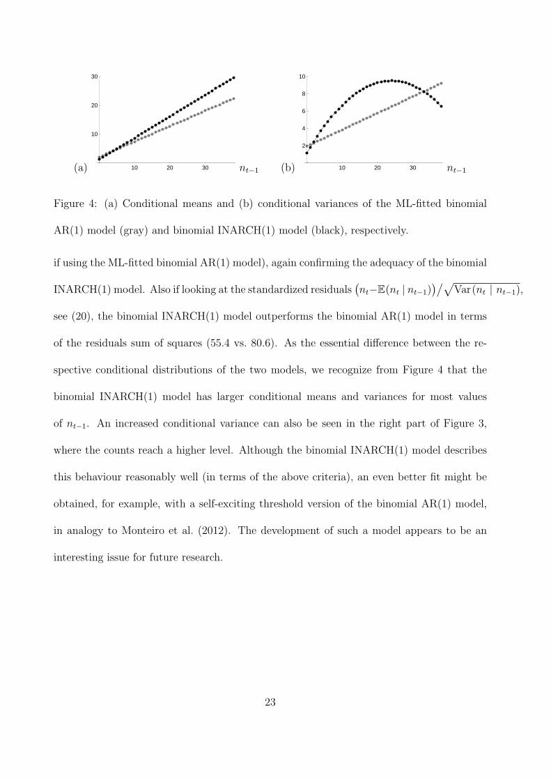
Figure 4: (a) Conditional means and (b) conditional variances of the ML-fitted binomial

AR(1) model (gray) and binomial INARCH(1) model (black), respectively.

if using the ML-fitted binomial AR(1) model), again confirming the adequacy of the binomial

INARCH(1) model. Also if looking at the standardized residuals(nt−E(nt | nt−1)

)/√Var(nt | nt−1),

see (20), the binomial INARCH(1) model outperforms the binomial AR(1) model in terms

of the residuals sum of squares (55.4 vs. 80.6). As the essential difference between the re-

spective conditional distributions of the two models, we recognize from Figure 4 that the

binomial INARCH(1) model has larger conditional means and variances for most values

of nt−1. An increased conditional variance can also be seen in the right part of Figure 3,

where the counts reach a higher level. Although the binomial INARCH(1) model describes

this behaviour reasonably well (in terms of the above criteria), an even better fit might be

obtained, for example, with a self-exciting threshold version of the binomial AR(1) model,

in analogy to Monteiro et al. (2012). The development of such a model appears to be an

interesting issue for future research.

23

5 Special Case: AModel with Density-Dependent Coloni-

sation

We concluded our earlier article (Weiß & Pollett, 2012) by referring briefly to the case α(y) =

α ∈ (0; 1), constant, and β a continuous, increasing and concave function with range in [0;α].

Such a model assumption is motivated by certain metapopulations with a density-dependent

colonisation probability and a fixed local extinction probability, and epidemic models with

a density-dependent infection probability and a fixed per-capita recovery probability.

5.1 Definition and Stochastic Properties

Let α(y) = α ∈ (0; 1) be constant, and let β be a linear function with range in [0;α], say,

β(y) = α (a+ by) with a, a+ b ∈ (0; 1]. Then (see Definition 2.1),

nt = α ◦ nt−1 + βt ◦ (N − nt−1),

which has an intuitive interpretation, for instance, in the epidemic context: if b > 0, the

probability that a susceptible becomes infected increases if the number of infectives in the

population is already large (the infection is spreading), while the recovery from the infection

is independent of other infectives.

If α(y) = α and β(y) = α (a+ by), then the following relations hold:

r(y) = α− β(y) = α (1− a− by), π(y) =β(y)

1− r(y)=

β(y)

1− α + β(y). (21)

24

Hence, the regression properties of formula (2) simplify to

E(nt | nt−1) = (α− βt)nt−1 +N βt,

Var(nt | nt−1) = (α− βt) (1− α− βt)nt−1 +N βt(1− βt).

(22)

If β is a linear function, then E(nt | nt−1) will be a quadratic polynomial in nt−1, and

Var(nt | nt−1) will be a cubic polynomial in nt−1. So we cannot proceed as in Theorem 4.1.2

to obtain closed-form expressions for stationary mean or variance.

From now on, we focus on the stationary case again (see Section 2.1). While (22) does

not allow us this time to obtain closed-form expressions for stationary mean or variance, we

can at least derive a variance-mean relation: since E(nt | nt−1) = α(1− a− b nt−1/N)nt−1 +

Nα (a+ b nt−1/N), we have

µ = Nαa+ α(1− a+ b)µ− αb/N (σ2 + µ2). (23)

Given concrete values for the model parameters a, b and α, the exact mean, variance and

autocorrelation function can be computed numerically according to the procedure laid out

in Section 2.1; see also the discussion below.

General closed-form approximations are now derived using formula (9). The functions

f(x) and v(x) according to formulae (3) and (4) are obtained as

f(x) = αx + α (a+ bx) (1− x) = α(a+ (1− a+ b) x− b x2

),

f ′(x) = α (1− a+ b− 2b x),

v(x) = α(1− α) x + α (a+ bx)(1− α (a+ bx)

)(1− x).

(24)

25

Lemma 5.1.1. If b = 0, then the unique fixed point of f in [0; 1] is

x∗ =1− α (1− a+ b) −

√(1− α (1− a+ b)

)2+ 4α2ab

−2αb∈ (0; 1).

If b = 0 (no density dependence), then x∗ = αa/(1− α(1− a)

)∈ (0; 1).

The proof is given in Appendix A.3.

Using Lemma 5.1.1 and formula (24), we obtain

κ = f ′(x∗) = α (1− a+ b)− 2bα x∗ = 1−√(

1− α (1− a+ b))2

+ 4α2ab, (25)

which also holds for b = 0, since 1 − α(1 − a) ∈ (0; 1]. So we can compute approximations

for stationary mean µ, variance σ2 and autocorrelation function ρ(k) using formula (9).

We performed numerical experiments to test the quality of this approximation; results

are summarized in Table 3. Model parametrizations were chosen so that different levels of

the mean µ/N (about 0.15 or 0.40), of the index of dispersion Id (about 1.1 or 1.5), and of

the ρ(1) (about 0.4 or 0.8) were covered. For each parametrization we computed

• numerically exact values for a range of N values (as described in Section 2.1) and

• large–N approximations (rows “N = ∞” in Table 3).

From the tabulated values, it is apparent that the approximations are quite accurate, at

least for N ≥ 25. If the stationary distribution is only slightly overdispersed, then even

when N = 5 the approximation is good.

5.2 Parameter Estimation

We follow the programme of Section 4.2. For the model described in Section 5.1, the functions

α and β, and hence Pθ(k|l), are also polynomials in the model parameters, and therefore

26

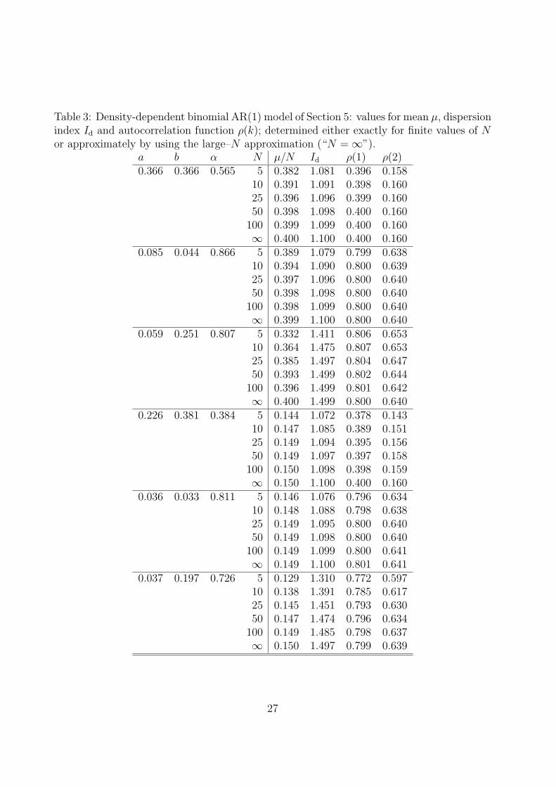
Table 3: Density-dependent binomial AR(1) model of Section 5: values for mean µ, dispersionindex Id and autocorrelation function ρ(k); determined either exactly for finite values of Nor approximately by using the large–N approximation (“N = ∞”).

a b α N µ/N Id ρ(1) ρ(2)0.366 0.366 0.565 5 0.382 1.081 0.396 0.158

10 0.391 1.091 0.398 0.16025 0.396 1.096 0.399 0.16050 0.398 1.098 0.400 0.160100 0.399 1.099 0.400 0.160∞ 0.400 1.100 0.400 0.160

0.085 0.044 0.866 5 0.389 1.079 0.799 0.63810 0.394 1.090 0.800 0.63925 0.397 1.096 0.800 0.64050 0.398 1.098 0.800 0.640100 0.398 1.099 0.800 0.640∞ 0.399 1.100 0.800 0.640

0.059 0.251 0.807 5 0.332 1.411 0.806 0.65310 0.364 1.475 0.807 0.65325 0.385 1.497 0.804 0.64750 0.393 1.499 0.802 0.644100 0.396 1.499 0.801 0.642∞ 0.400 1.499 0.800 0.640

0.226 0.381 0.384 5 0.144 1.072 0.378 0.14310 0.147 1.085 0.389 0.15125 0.149 1.094 0.395 0.15650 0.149 1.097 0.397 0.158100 0.150 1.098 0.398 0.159∞ 0.150 1.100 0.400 0.160

0.036 0.033 0.811 5 0.146 1.076 0.796 0.63410 0.148 1.088 0.798 0.63825 0.149 1.095 0.800 0.64050 0.149 1.098 0.800 0.640100 0.149 1.099 0.800 0.641∞ 0.149 1.100 0.801 0.641

0.037 0.197 0.726 5 0.129 1.310 0.772 0.59710 0.138 1.391 0.785 0.61725 0.145 1.451 0.793 0.63050 0.147 1.474 0.796 0.634100 0.149 1.485 0.798 0.637∞ 0.150 1.497 0.799 0.639

27

differentiable up to any order. To check (ii), we consider the Jacobian of (17) with θ =

(a, b, α)⊤, α(y) = α and β(y) = α(a + by). Its determinant is obtained (after tedious

computations) as

(N − 1)α3 (1− αa)N−1(1− (a+ b/N)

) (1− α(a+ b/N)

)2(N−2).

Again, provided N > 1, this determinant is not equal to 0, implying that Jacobian of (17)

has full rank, which, in turn, implies that (ii) holds.

Concerning the MM approach discussed in Remark 2.2.1, we are now in a situation

where no closed-form expressions for the moments are available. However, an approximate

MM approach by way of the large–N approximation of moments derived in Section 3.3 is

possible: using formula (9) together with formulae (24) and (25), as well as Lemma 5.1.1,

closed-form approximations for mean, variance and first-order autocorrelation follow, which

can be obtained for the model parameters a, b and α.

6 Conclusion

We have considered a generalization of the binomial AR(1) process nt with range {0, 1, . . . , N},

where the model parameters are not constant in time, but rather depend on the current den-

sity nt/N . We were able to derive a law of large numbers and a central limit theorem, which

can be applied to obtaining large–N approximations for various quantities of interest. The

utility of our approach was demonstrated by considering two particular subfamilies of the

density-dependent binomial AR(1) model. The models discussed in Section 4 permit a wide

range of over- and underdispersion scenarios, a valuable feature in practice, as illustrated

by the real-data examples of securities counts and infection counts. The model presented

28

in Section 5 is motivated by metapopulations with density-dependent colonisation and a

fixed extinction probability, and epidemic models with density-dependent infection and a

fixed per-capita recovery probability. It was useful in helping to illustrate the quality of our

large–N approximations.

An important issue for future research will be the development of statistical procedures

for model identification and diagnostics for density-dependent binomial autoregressive mod-

els. Different forms of state-dependence will also be investigated, including a self-exciting

threshold version of the binomial AR(1) model, in analogy to Monteiro et al. (2012) and

motivated by Example 4.3.1. Future research will focus on the binomial INARCH(1) model

introduced in Section 4.3. Extensions to higher-order autoregressions and time-varying pop-

ulation ceiling Nt will also be considered. Finally, an extension of (density-dependent)

binomial autoregressive models to negative integer values will be explored, for example, by

using a signed binomial thinning operation, as in Kim & Park (2008).

Acknowledgements

The work of Phil Pollett is supported by the Australian Research Council (Discovery grant DP120102398,

and the Centre of Excellence for Mathematics and Statistics of Complex Systems). The authors

thank the editor, the co-editor, and the two referees for carefully reading the article and for their

comments, which greatly improved the article. The authors are also grateful to Prof. Hee-Young

Kim, Korea University, for contributing the securities counts data of Example 4.2.1.

29

References

Al-Osh, M.A., Alzaid, A.A. (1991) Binomial autoregressive moving average models. Communica-

tions in Statistics – Stochastic Models 7(2), 261–282.

Billingsley, P. (1961) Statistical Inference for Markov Processes. University of Chicago Press.

Buckley, F.M., Pollett, P.K. (2009) Analytical methods for a stochastic mainland-island metapopu-

lation model. In Proceedings of the 18th World IMACS Congress and MODSIM09 International

Congress on Modelling and Simulation, R. Anderssen, R. Braddock, and L. Newham, Eds. Mod-

elling and Simulation Society of Australia and New Zealand and International Association for

Mathematics and Computers in Simulation, Canberra, Australia, 1767–1773.

Buckley, F.M., Pollett, P.K. (2010a) Limit theorems for discrete-time metapopulation models.

Probability Surveys 7, 53–83.

Buckley, F.M., Pollett, P.K. (2010b) Analytical methods for a stochastic mainland-island metapop-

ulation model. Ecological Modelling 221(21), 2526–2530.

Cui, Y., Lund, R. (2010) Inference in binomial AR(1) models. Statistics and Probability Letters

80(23-24), 1985–1990.

Daley, D., Gani, J. (1999) Epidemic Modelling: an Introduction. Cambridge Studies in Mathemat-

ical Biology, Vol. 15. Cambridge University

Ferland, R., Latour, A., Oraichi, D. (2006) Integer-valued GARCH processes. Journal of Time

Series Analysis 27(6), 923–942.

Hagmark, P.-E. (2009) A new concept for count distributions. Statistics and Probability Letters

79(8), 1120–1124.

30

Kim H.-Y., Park, Y. (2008) A non-stationary integer-valued autoregressive model. Statistical Papers

49(3), 485–502.

McKenzie, E. (1985) Some simple models for discrete variate time series. Water Resources Bulletin

21(4), 645–650.

Monteiro, M., Scotto, M.G., Pereira, I. (2012) Integer-valued self-exciting threshold autoregressive

processes. Communications in Statistics – Theory and Methods 41(15), 2717–2737.

Robert Koch-Institut (2013) SurvStat@RKI http://www3.rki.de/SurvStat, data status: June

12, 2013.

Steutel, F.W., van Harn, K. (1979) Discrete analogues of self-decomposability and stability. Annals

of Probability 7(5), 893–899.

Triebsch, L.K. (2008) New Integer-valued Autoregressive and Regression Models with State-

dependent Parameters. Doctoral dissertation, TU Kaiserslautern, Verlag Dr. Hut, Munich.

Weiß, C.H. (2009) Monitoring correlated processes with binomial marginals. Journal of Applied

Statistics 36(4), 399–414.

Weiß, C.H. (2010) The INARCH(1) model for overdispersed time series of counts. Communications

in Statistics – Simulation and Computation 39(6), 1269–1291.

Weiß, C.H., Kim, H.-Y. (2013a) Binomial AR(1) processes: moments, cumulants, and estimation.

Statistics 47(3), 494–510.

Weiß, C.H., Kim, H.-Y. (2013b) Parameter estimation for binomial AR(1) models with applications

in finance and industry. Statistical Papers 54(3), 563–590.

31

Weiß, C.H., Pollett, P.K. (2012) Chain binomial models and binomial autoregressive processes.

Biometrics 68(3), 815–824.

A Proofs

A.1 Proofs of Section 2

Since

αt(1− αt)− βt(1− βt) = (αt − βt) (1− αt − βt) = rt (1− rt − 2βt),

we obtain

E(nt | nt−1) = E(αt ◦ nt−1 | nt−1) + E(βt ◦ (N − nt−1) | nt−1

)= (αt − βt)nt−1 +N βt = rt nt−1 +N βt,

Var(nt | nt−1) = Var(αt ◦ nt−1 | nt−1) + Var(βt ◦ (N − nt−1) | nt−1

)=

(αt(1− αt)− βt(1− βt)

)nt−1 +N βt(1− βt)

= rt(1− rt) (1− 2πt)nt−1 +N βt(1− βt),

so formula (2) follows.

32

A.2 Proofs of Section 4

From formula (2), we obtain

E(nt | nt−1) = r nt−1 +N(1− r)πt =(r + (1− r)b

)nt−1 +N(1− r)a,

Var(nt | nt−1) = r(1− r) (1− 2πt)nt−1 +N(1− r)πt(1− (1− r)πt

)= r(1−r)

N (N(1− 2a)− 2b nt−1)nt−1

+ 1−rN (Na+ b nt−1)

(N −N(1− r)a− (1− r)b nt−1

)= r(1− r)(1− 2a)nt−1 − 2b r(1−r)

N n2t−1 + N(1− r)a

(1− (1− r)a

)+ b(1− r)

(1− 2(1− r)a

)nt−1 − (1−r)2 b2

N n2t−1

= N(1− r)a(1− (1− r)a

)− b(1−r)

N

(2r + b(1− r)

)n2t−1

+ (1− r)((1− 2a)(b+ r) + 2abr

)nt−1.

For k-step regressions with k = 1, . . . , t, we argue by induction:

E(nt | nt−k) = E(E(nt | nt−1, . . . , nt−k)

∣∣ nt−k

)=

(r + (1− r)b

)E(nt−1 | nt−k) +N(1− r)a

= . . . =(r + (1− r)b

)knt−k + N(1− r)a

∑k−1i=0

(r + (1− r)b

)i=

(r + (1− r)b

)knt−k + N(1− r)a

1−(r+(1−r)b

)k(1−r)(1−b) ,

from which we obtain (11). Hence, the assertion of Theorem 4.1.1 follows.

Next, we consider Theorem 4.1.2. From (12), the mean µ = E(nt) satisfies

µ = E(E(nt | nt−1)

)=

(r + (1− r)b

)µ+N(1− r)a.

Solving for µ, we obtain formula (13).

33

For the variance σ2 = Var(nt), the relation

σ2 = E(Var(nt | nt−1)

)+Var

(E(nt | nt−1)

)= N(1− r)a

(1− (1− r)a

)− b(1−r)

N

(2r + b(1− r)

)(σ2 + µ2)

+ (1− r)((1− 2a)(b+ r) + 2abr

)µ +

(r + (1− r)b

)2σ2

= (1− r)(1− b)(1− (1− r)a

)µ + (1− r)

((1− 2a)(b+ r) + 2abr

)µ

− ab1−r1−b

(2r + b(1− r)

)µ +

(r + (1− r)b

)2σ2 − 1

N

((r + b(1− r)

)2 − r2)σ2

= 1−a−b1−b (1− r2)µ +

(r2

N + (1− 1N )

(r + (1− r)b

)2)σ2

holds. Using 1− µ/N = 1−a−b1−b , formula (14) follows, and the proof of Theorem 4.1.2 is complete.

For Remark 4.1.3, we consider the following partial derivative:

∂∂b Id(N, b, r) = 0 iff −(1 + r)

(− 2(1− 1

N )r − 2(1− 1N )(1− r)b

)= 0

iff r + (1− r)b = 0 iff b = −r1−r .

Finally, we have to prove formula (16): we obtain from formula (12) and for k ≥ 1 that

Cov[nt, nt−k] = Cov[E(nt | nt−1, . . .), E(nt−k | nt−1, . . .)

]= Cov

[(r + (1− r)b

)nt−1 +N(1− r)a, nt−k

]=

(r + (1− r)b

)Cov[nt−1, nt−k] = . . . =

(r + (1− r)b

)kσ2.

A.3 Proof of Lemma 5.1.1

The function g(x) = f(x)−x = αa−(1−α (1−a+b)

)x−αb x2 is a quadratic polynomial (if b = 0)

with g(0) = αa > 0 and g(1) = −(1− α) < 0. Hence, there is a unique root in (0; 1). b determines

the sign of the quadratic term. If b < 0, the smaller one of the two roots of g(x) is in (0; 1), for

b > 0, it is the larger one.

The roots of g(x) are given by

x1,2 =1− α (1− a+ b) ±

√(1− α (1− a+ b)

)2+ 4α2ab

−2αb,

34

so

x2 − x1 =

√(1− α (1− a+ b)

)2+ 4α2ab

αb.

Therefore, x2 < x1 if b < 0 and x2 > x1 if b > 0, that is, x2 is the unique root in (0; 1).

35