biochemistry: enzyme kinetics title page · introduction the derivation of the... non-... modeling...

Introduction

The Derivation of the . . .

Non- . . .

Modeling Bacterial . . .

Home Page

Title Page

JJ II

J I

of 28

Go Back

Full Screen

Close

Quit

Biochemistry: Enzyme Kinetics

Aaron Flores and Chris Chun

February 22, 2012

Introduction


Non- . . .


Home Page

Title Page

JJ II

J I

Page 1 of 28

Go Back

Full Screen

Close

Quit

Abstract

The aim of this paper is to help demonstrate how to model microbial reproduction with-in a chemostat using systems of ordinary differential equation. This paper shall first derivethe Michaelis-Menten equation outlined by the quasi steady state hypothesis using two differentways: one more algebraically intuitive and the other, a more calculus heavy derivation. Althoughfor the aim and scope of this paper, it doesn’t extend into more complicated models of theMichaelis and Menten equation, we shall however show a non-dimensionalized Michaelis Mentenequation although it will not be necessary in understanding our simple model of the chemostat.Lastly we shall investigate the stability of the system. It is assumed that the reader has generalknowledge about ODE’s and classification of equilibrium points and eigenvalues, and is to becomfortable differentiating and integrating.

Introduction


Non- . . .


Home Page

Title Page

JJ II

J I

Page 1 of 28

Go Back

Full Screen

Close

Quit

Introduction

The field of enzymology is very complex, requiring a strong base understanding of generalbiology and chemistry. Our human body has tissues protecting the exposure of our muscles,bones and organs, etc. These parts too are made up of even smaller units of life which we callcells. Just beyond this micro level is a war of molecules colliding together. At this molecularlevel enzymes bind to their married substrates to form proteins. Throughout the human body,this event or synthesis explains how we are able to metabolize, form scabs to heal from aninjury, digest food, grow hair, and countless other activities are all governed by reactions thatrequire catalyst. In modern day society it seems that scientific breakthroughs have revealed nolimits to the extent at which Biology, Chemistry and Mathematics coincide amongst all aspectsof life. In Biochemistry the subject of enzymology : the study of dynamic interactions betweenenzymes and their substrates, allows us to observe the behavior of the enzymes present in acell membrane. In 1835 the first studies of these substances were conducted by Jons Berzellius,who insisted that these substances be called catalysts. A catalyst is a substance that can beintroduced to a compound in order for it to undergo a chemical reaction, where either thecatalyst reduces or strengthens the amount of activation energy needed to react. Even thoughthe catalyst experiences reaction, itself does not change. The term enzyme would not comeuntil 41 years later purposed by Willy Kuhne. Enzymes specifically are protein catalyst thatbind to a specific substrate to react with to form a product. The roots of this word come fromthe latin term “enzymos” meaning “in yeast”. In this research paper we will address events atthe molecular level, use the application of Michaelis-Menten kinetics to understand and modelbacterial growth in a Chemostat.

The Derivation of the Michaelis-Menten model of EnzymeKinetics

Here we begin our first attempt at deriving the Michaelis-Menten model of Enzyme kinetics.

S + Ek1−−−⇀↽−−−k−1

SEcomplex

k2−→ P + E (1)

Introduction


Non- . . .


Home Page

Title Page

JJ II

J I

Page 2 of 28

Go Back

Full Screen

Close

Quit

where S, E, and P denotes a substrate S, an enzyme E, and protein P. k1,k−1,and k2 are theassociated rates of change at which the reactions occur. This equation can be interpreted as asubstrate S and an Enzyme E combine to form a complex SE at which either it can produce aproduct P and release enzyme E or have a retrograde reaction into it’s previous components Sand E.

The Michaelis-Menten model seeks to find the maximum rate at which a given concentrationof a substrate [S] and enzyme [E] can combines to form a product P, assuming the substrateto be in excess comparatively to the enzyme . We use [ ] to denote concentration and V shallrepresent the the rate of reproduction of a certain a concentration of product [P]

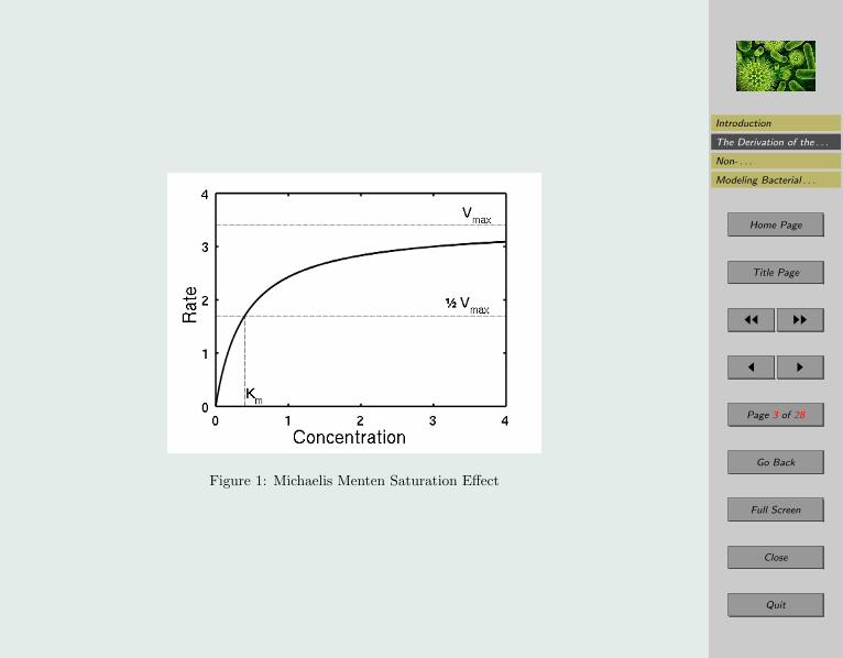
Prior to any quantitative analysis regarding the velocity V, at which the rate of reaction occursfrom substrate to protein, it is necessary to apply some qualitative analysis regarding the maththat is to model this molecular event. In theory if the enzyme is taken to be the limiting reactantand the substrate to be the excess, we should expect that the substrate would combine with theenzymes quite rapidly until there was a point where every enzyme has already combined witha substrate leaving no other bonding sites for a substrate to combine with an enzyme. Therefor an ordinary differential equation is a suitable model of this scenario because we are relatingrates of change with in the concentrations relative to their initial concentrations. We shouldexpect the graph of this behavior to have this form:

Notice how the rate increases very quickly as the concentration of the substrate is low but thanstarts to decrease gradually where it then approaches a maximum velocity asymptotically asthe concentration increases (see Figure 1).

Understanding that these conditions only persist in the case where the excess reactant isthe substrate and the limiting reactant is the enzyme, is very crucial before any further anal-ysis because under this assumption that the substrate is in the excess, allows us to interpretequation (1) as going only one way, that is from substrate to product, therefore directing ourattention to the rate at which a complex forms a product defined by k2 shall be the primaryfocus of the model. This is denoted by :

Introduction


Non- . . .


Home Page

Title Page

JJ II

J I

Page 3 of 28

Go Back

Full Screen

Close

Quit

Figure 1: Michaelis Menten Saturation Effect

Introduction


Non- . . .


Home Page

Title Page

JJ II

J I

Page 4 of 28

Go Back

Full Screen

Close

Quit

V = k2[SE] (2)

k2[SE] = k1[S][E]− k−1[SE]

combining like terms gives

k2[SE] + k−1[SE] = k1[S][E]

[SE] =k1[S][E]

k2 + k−1(3)

Now introduce a new constant Km which we define as:

Km =k2 + k−1

k1(4)

Km is know as the Michaelis constant. Substituting this value into equation (3) gives:

[SE] =[S][E]

Km(5)

Understanding that the concentration of free enzymes is equivalent to the initial concentrationof enzyme subtracted from the concentration of enzymes that have bonded with a substrate toform a substrate enzyme complex [SE] allows to rewrite E as:

[E] = [Eo]− [SE] (6)

Substituting this value of E given by (6) into equation (5) and solving for the concentration

Introduction


Non- . . .


Home Page

Title Page

JJ II

J I

Page 5 of 28

Go Back

Full Screen

Close

Quit

of the complex [SE] gives:

[SE] =[S]([Eo]− [SE])

Km

[SE] =[S][Eo]

Km− [S][SE]

Km

[SE] +[S][SE]

Km=

[S][Eo]

Km

[SE]

(1 +

[S]

Km

)=

[S][Eo]

Km

SE =[S][Eo]

Km + [S](7)

Now substitute this value of [SE] into equation (2) resulting in:

V = k2[S][Eo]

Km + [S]

Remembering assumption that the concentration of substrate is far greater than the concentra-tion of enzymes allows us to simplify further. If [S]� [E], then Vmax = k2[Eo]. That is to saythe maximum velocity a substrate of given concentration is able to produce a product is limitedby the initial concentration of enzymes assuming [S]� [E]. Therefore

V =Vmax[S]

Km + [S]

This method is very light on the calculus work. There are of course other methods thatuse systems of of ordinary differential equations to solve for the velocity of the reaction rate. Ithought that this derivation however was the easiest to understand.

Now here is a more calculus heavy derivation:recall equation (1)

S + Ek1−−−⇀↽−−−k−1

SEcomplex

k2−→ P + E

Introduction


Non- . . .


Home Page

Title Page

JJ II

J I

Page 6 of 28

Go Back

Full Screen

Close

Quit

Again reading this as one molecule of substrate S combines with one molecule of enzyme Eto react at a rate k1 to form one molecule of a complex SE at which either it can produce onemolecule of product and one molecule of enzyme at a rate of k2 or have a reverse reaction at arate of k−1 where it decomposes into it’s original components. The law of mass action statesthat the rate of reaction is proportional to the concentration of the reactants. We shall denotethe concentration of these various molecules with lowercase letters as follows:

e = [E] s = [S] c = [SE] p = [P ]

Applying the law of mass action yields the following system of four ordinary differential equa-tions:

ds

dt= −k1es+ k−1c (8)

In this case k1 is negative because the complex is decomposing which is why k−1 is positive.

de

dt= −k1es+ (k−1 + k2)c (9)

In this case we must also include k2 because the complex can either decompose or produce Pand E via k2.

dc

dt= k1es− (k−1 + k2)c (10)

In this case the decomposition is understood to be a negative rate as an increase in this rateleads to a lesser concentration of complex,and I believe the last one to be the most obvious.

dp

dt= k2c (11)

Notice thatde

dt+dc

dt= 0 =⇒ e+ c = eo

With some intuitive reasoning it easy to derive our initial conditions. At time zero where noreaction has occurred we should expect to have no product and no complex while the enzymeand substrate concentration should remain at their initial concentrations:

e(0) = eo s(0) = so c(0) = 0 p(0) = 0

Introduction


Non- . . .


Home Page

Title Page

JJ II

J I

Page 7 of 28

Go Back

Full Screen

Close

Quit

Replacing e with eo − c into (8) and (10) gives:

ds

dt= −k1eos+ (k1s+ k−1)c (12)

dc

dt= k1eos− (k1s+ k−1 + k2)c (13)

It is generally thought the rate at which the complex forms is to be quite rapid after which it isassumed to virtually have no velocity therefore it is appropriate to say that the rate at whichthe complex changes with respect to time is roughly equal to zero. That is ;

dc

dt≈ 0

This is known as the quasi-steady-state hypothesis Substituting for this approximation into(13)

c =k1eos

k1s+ k−1 + k2

introducing the Michaelis constant

Km =k2 + k−1

k1

yields:

c =k1seo

k1s+k1 (k−1 + k2)

k1

c =k1seo

k1

(s+

k−1 + k2k1

)c =

seos+Km

(14)

Introduction


Non- . . .


Home Page

Title Page

JJ II

J I

Page 8 of 28

Go Back

Full Screen

Close

Quit

substituting this value into (14)

ds

dt= −k1eos+ (k1s+ k−1)c

ds

dt=−k1seo(s+Km)

s+Km+

(k1s+ k−1)seos+Km

ds

dt=

seos+Km

(−k1Km + k−1)

ds

dt=

seos+Km

(−k1

(k−1 + k2

k1

)+ k−1

)ds

dt=

seos+Km

(−k−1 − k2 + k−1)

ds

dt=−k2seos+Km

(15)

solving for dp/dt is a lot easier:

(16)

dp

dt= k2c ⇒

dp

dt=

k2seos+Km

The growth rate of the product is a function of substrate availability. Therefore the maximumrate at which the reaction occurs is limited by the initial enzyme concentration if s >> p.Incorporating this into our model finially gives:

ds

dt= − Vmaxs

s+Km,dp

dt=

Vmaxs

s+Km

(17)

Which is what we got without all that calculus stuff in the first derivation

Introduction


Non- . . .


Home Page

Title Page

JJ II

J I

Page 9 of 28

Go Back

Full Screen

Close

Quit

Non-dimensionalization of Michaelis-Menten

Although this answer is a good approximation of the general behavior of the complex it is onlyfairly accurate over the ”long” time scale. However we can increase accuracy by recognizingthat the system occurs over two time scales and putting the equation into a non-dimensionalunit-less form.

Introducing the following dimensionless quantities :

τ = k1eot, u(τ) =s(t)

so, v(τ) =

c(t)

eo

λ =k2k1so

, K =k−1 + k2k1So

=Km

so, ε =

eoso

Substituting these values into (12) and (13) transforms ds/dt and dc/dt respectively:

du

dτ= −u+ (u+K − λ)v, ε

dv

dτ= u− (u+K)v

u(0) = 1, v(0) = 0

This is easy to verify:

ds

dt= −k1eos+ (k1s+ k−1)c V

du

dτ= −u+ (u+K − λ)v

Introduction


Non- . . .


Home Page

Title Page

JJ II

J I

Page 10 of 28

Go Back

Full Screen

Close

Quit

Using the chain rule,

du

dτ=du

ds× ds

dt× dt

dτ(18)

Next,

t =τ

k1e0⇒ dt

dτ=

1

k1eo(19)

And,

u =s

so⇒ du

ds=

1

so(20)

Now we have everything to do this. Pluging (19) , (20) ,and (12) into (18) gives:

du

dτ=

(1

so

)(−k1eos+ (k1s+ k−1)c)

(1

k1eo

)du

dτ=−k1eosk1eoso

+(k1s+ k−1)c

(k1so)eo

du

dτ=−sso

+

(k1s

k1so+k−1k1so

)c

eo

du

dτ=−sso

+

(s

so+k−1 + k2k1so

− k2k1so

)c

eodu

dτ= −u+ (u+K − λ)v

Introduction


Non- . . .


Home Page

Title Page

JJ II

J I

Page 11 of 28

Go Back

Full Screen

Close

Quit

Now solving for dv/dτ :

dv

dτ=dv

dc× dc

dt× dt

dτ(21)

v =c

eo⇒ dv

dc=

1

eo(22)

Plug (22) , (13) , and (19) , intro (21)

dv

dτ=

1

eo(k1eos− (k1s+ k−1 + k2)c)

1

k1eo

dv

dτ=k1eos

k1e2o− (k1s+ k−1 + k2)c

k1e2o

dv

dτ=

s

eo−(k1s+ k−1 + k2

k1eo

)(c

eo

)dv

dτ=

s

eo−(k1s

k1eo+k−1 + k2k1eo

)(c

eo

)dv

dτ=

s

eo−(s

eo+k−1 + k2k1eo

)(c

eo

)(23)

Therefore multiplying equation (23) by ε = eo/so we arrive at the following result

εdv

dτ=eoso

[s

eo−(s

eo+k−1 + k2k1eo

)(c

eo

)]εdv

dτ=

s

so−(s

so+k−1 + k2k1so

)(c

eo

)εdv

dτ= u− (u+K)v (24)

Introduction


Non- . . .


Home Page

Title Page

JJ II

J I

Page 12 of 28

Go Back

Full Screen

Close

Quit

Modeling Bacterial Growth in Chemostat

Now that we have derived the Michaelis-Menten Model of enzyme kinetics, we can now use itto investigate the growth of bacteria. A Chemostat is a device used in a laboratory to producea bacterial culture in such way that the culture’s nutrients are replenished so that continuousharvesting is possible in convenient quantities. The environmental factors contributing to repro-duction are kept under control for optimization of harvest. Because these various parametersare kept under control our simple model of Michaelis-Menten derived from the quasi steadystate hypothesis is a suitable model enough for the purposes of analyzing bacterial growth ina chemostat and is therefore it is not necessary to have a non-dimensionalized version of theequation. Refer to Figure 2 for diagram of chemostat.

Assumptions

1. Solutions are homogenous in each tank meaning that the consistency and concentrationis kept the same throughout.

2. The Nutrient is the excess reactant so the way it interacts with the bacteria is similarto the way substrates react with enzymes like in the Michaelis-Menten model of enzymekinetics.

3. Nutrient depletion occurs continuously as a result of reproduction which we will denoteas the yield constant α which is to say α units of nutrient are consumed in producing oneunit of bacterial population.

Introduction


Non- . . .


Home Page

Title Page

JJ II

J I

Page 13 of 28

Go Back

Full Screen

Close

Quit

Figure 2: Basic Diagram of Chemostat

Introduction


Non- . . .


Home Page

Title Page

JJ II

J I

Page 14 of 28

Go Back

Full Screen

Close

Quit

The rate at which the the bacterial population is growing will be determined by the rate itreproduces itself versus the rate it is lost to the effluent. Because the rate at which the bacteriareproduces itself is a function of nutrient availability and has the same behavior as seen in thesaturating affect of enzymes on substrates, we use K(N) which we defined earlier as V anddp/dt. It represents the ”Michaelis function”.

dB

dt= K(N)B − F

VB (25)

dN

dt= −αK(N)B − F

VN +

F

VNo (26)

Also, in order to quantify the change in the nutrient and bacterial population density we to needknow how much is lost by the flow rate F relative to the population density of each substancein each container, remembering that density is mass/volume . Substituting what we previouslyderived for K(N) gives:

dB

dt=

KmaxN

Kn +NB − F

VB (27)

dN

dt= −αKmaxN

Kn +NB − F

VN +

F

VNo (28)

Now that we have an appropriate model it is important to increase accuracy by putting themodel into a dimensionless form so that the model stays consistent despite a possible changein units. This ensures that the result produced is accurate as long as the units of measurementare consistent with that by which they measure: for example units used to measure volumeshould be used for volumes and units of length should be used for units of length. It would benonsensical to measure the volume of liquid in seconds.

Introduction


Non- . . .


Home Page

Title Page

JJ II

J I

Page 15 of 28

Go Back

Full Screen

Close

Quit

The common method of non-dimensionalization of a system is to first realize that any unitdimension can be interpreted as a scalar multiple j* × a unit-vector j carrying dimension. Thisunderstanding is powerful because it allows us to further simplify our equation. Solving fordB/dt :

d(B∗B)

d(t∗τ)=

(KmaxN

∗N

Kn +N∗N

)B∗B − F

V(B∗B)

d(B∗B)

d(t∗)= τ

(KmaxN

∗N

Kn +N∗N

)B∗B − τF

V(B∗B)

d(B∗)

d(t∗)= τ

(KmaxN

∗N

Kn +N∗N

)B∗ − τF

V(B∗)

d(B∗)

d(t∗)= τKmax

N∗NNKn

N+N∗N

B∗ − τFVB∗

d(B∗)

d(t∗)= τKmax

(N∗

Kn

N+N∗

)B∗ − τF

VB∗ (29)

Introduction


Non- . . .


Home Page

Title Page

JJ II

J I

Page 16 of 28

Go Back

Full Screen

Close

Quit

Solving for dN/dt gives:

d(N∗N)

d(t∗τ)= −α

(KmaxN

∗N

Kn +N∗N

)B∗B − F

V(N∗N) +

F

VNo

d(N∗N)

d(t∗)= −τα

(KmaxN

∗N

Kn +N∗N

)B∗B − τF

V(N∗N) + τ

F

VNo

d(N∗)

d(t∗)= −ατ

N

(KmaxN

∗N

Kn +N∗N

)B∗B − τF

V(N∗) + τ

F

V

No

N

d(N∗)

d(t∗)= B

(−ατKmaxN

N

)(N∗

Kn

N+N∗

)B∗ − τF

VN∗ +

τFNo

V N(30)

Making a few choice substitutions allows further simplification of the system:

τ =V

F, N = Kn, B =

Kn

ατKmax

α1 = (τKmax) =V Kmax

F

α2 =τFNo

V N=NoKn

Now the system can be written as:

dB

dt= α1

(N

1 +N

)B −B (31)

dN

dt= −

(N

1 +N

)B −N + α2 (32)

Now the system has only two dimensionless quantities α1 and α2 instead of the original six (Kn , Kmax , F , V , No and α). Now we can solve for the steady state solution. By setting (31)

Introduction


Non- . . .


Home Page

Title Page

JJ II

J I

Page 17 of 28

Go Back

Full Screen

Close

Quit

and (32) equal to zero, we get:

α1

(N

1 +N

)B −B = 0 (33)

−(

N

1 +N

)B −N + α2 = 0 (34)

Equation (33) implies that either

N

1 +N=

1

α1or B = 0. (35)

If B = 0, then substituting B = 0 in equation (34) gives us

N = α2.

If B 6= 0, then we can solve solve the first of equations (35) to get:

N =1

α1 − 1

This result can be substituted in equation (34) to obtain:

B = α1(α2 −N)

Using this we derive two solutions to the non-linear homogeneous system:

(B1, N1) = (0,α2)

(B2, N2) =

(α1

(α2 −

1

α1− 1

),

1

α1 − 1

)We can however discard the first solution as is it is scientifically not interesting: no bacterialpopulation is left and the nutrient concentration is the same as the stock solution. The secondsolution looks more inspiring. Because there is no such thing as negative population densities

Introduction


Non- . . .


Home Page

Title Page

JJ II

J I

Page 18 of 28

Go Back

Full Screen

Close

Quit

B

N

1α1−1

(0,α2)

(α1

(α2 − 1

α1−1

), 1α1−1

)

Figure 3: Bacterial Nullclines.

it is intuitively obvious that α1 > 1 and like-wise α2 > 1/(α1 − 1). Inorder to understand thebehavior of the system we will begin by first graphing the nullclines to the non-linear homogenousODE and use it to classify the less scientifically interesting equilibrium point (B1, N1) and thenwe will use the Jacobian to evaluate the equilibrium point (B2, N2). We start first with theB nullclines as they are less challenging.From our previous anaylysis the bactereal nullclines isgiven by the constant solutions

B = 0

and

N =1

α1 − 1

This graph is shown in Figure 3.

Introduction


Non- . . .


Home Page

Title Page

JJ II

J I

Page 19 of 28

Go Back

Full Screen

Close

Quit

Interpreting Nutrient Nullclines

0 = −(

N

1 +N

)B −N + α2

−α2 +N = −(

N

1 +N

)B

−α2 +N

−B=

N

1 +N

−BN = (1 +N)(−α2 +N)

−B =(1 +N)(N − α2)

N

−B =N2 +N − α2N − α2

N

B = −N − 1 + α2 +α2

N

limN→∞

[B] = limN→∞

[−N − 1 + α2 +

α2

N

]B ≈ −N − 1 + α2

N ≈ −B + (α2 − 1)

In this form it is much easier to see that we are dealing with a hyperbola that has a horizontalasymptote at N = 0 and an oblique asymptote at N = −B + (α2 − 1) Where (B,N)⇔ (x, y)in Cartesian two-space. But we are not concerned with the negative parts of the graph asthere is no such thing as negative population densities. Limiting our attention to the positiveregion we recall that our other equilibrium point was at (0,α2). Because we discovered thatthere is horizontal asymptote at N = 0 we now know that the N null-cline that intersects at

Introduction


Non- . . .


Home Page

Title Page

JJ II

J I

Page 20 of 28

Go Back

Full Screen

Close

Quit

B

N

1α1−1

(0,α2)

(α1

(α2 − 1

α1−1

), 1α1−1

)

Figure 4: The Nutrient Nullcline.

(0,α2), which has no vertical motion along that null-cline, asymptotically approches zero as thebacterial population increases to infinity (see Figure 4).

Notice if B = 0 and N > α2 then dN/dt is negative which refers to the vertical motion.Likewise if N is less then α2 then dN/dt is positive, which seem to indicate stability but onlyalong the line B = 0. If however, B > 0 all possible trajectories are pulled away either to left orthe right because dB/dt (horizontal motion) is no longer equal to zero. This analysis indicatesthat at (B1, N1) there is a semi-stable saddle. However we still do not have enough informationto classify this equilibrium point, so we use the Jacobian to confirm our findings.

Introduction


Non- . . .


Home Page

Title Page

JJ II

J I

Page 21 of 28

Go Back

Full Screen

Close

Quit

This is the Jacobian of the Chemostat:

J(B,N) =

∂

∂B

[α1

(N

1 +N

)B −B

]∂

∂N

[α1

(N

1 +N

)B −B

]∂

∂B

[−(

N

1 +N

)B −N + α2

]∂

∂N

[−(

N

1 +N

)B −N + α2

]

The Jacobian evaluated at (B,N):

J(B,N) =

α1

(N

1 +N

)− 1

α1B

(1 +N)2

−(

N

1 +N

)−B

(1 +N)2 − 1

The Jacobian evaluated at (0,α2)

J(0,α2) =

α1

(α2

1 + α2

)− 1

α10

(1 + α2)2

−(

α2

1 + α2

)−0

(1 + α2)2 − 1

J(0,α2) =

α1α2

1 + α2− 1 0

−α2

1 + α2−1

∴ D = 1− α1α2

1 + α2

Introduction


Non- . . .


Home Page

Title Page

JJ II

J I

Page 22 of 28

Go Back

Full Screen

Close

Quit

First recall that inorder for this system to be valid certain condition on the parameters α1

and α2 must be satisfied. Again these conditions are as follows:

α1 > 1→ α1 − 1 > 0 ∴ α2 >1

α1 − 1> 0 (36)

Next we wish to find under what conditions the determinant is negative.

0 > D

0 > 1− α1α2

1 + α2

0 > 1 + α2 − α1α2

0 > 1 + α2(1− α1)

−1 > α2(1− α1)

1 < α2(α1 − 1)

1

α1 − 1< α2

Which is supported by our assumptions in (36) therefore without question we know that at(0,α2) we have a saddle

Next we evaluate the Jacobian at the equlirium point

(α1

(α2 −

1

α1 − 1

),

1

α1 − 1

)First recall that the Jacobain evaluated at (B,N) is

J(B,N) =

α1

(N

1 +N

)− 1

α1B

(1 +N)2

−(

N

1 +N

)−B

(1 +N)2 − 1

Introduction


Non- . . .


Home Page

Title Page

JJ II

J I

Page 23 of 28

Go Back

Full Screen

Close

Quit

=

α1

1

α1 − 1

1 +1

α1 − 1

− 1

α21

(α2 −

1

α1 − 1

)(

1 +1

α1 − 1

)2

−1

1

α1 − 1

1 +1

α1 − 1

−α1

(α2 −

1

α1 − 1

)(

1 +1

α1 − 1

)2 − 1

=

α1

1

α1 − 1α1 − 1 + 1

α1 − 1

− 1

α21

(α2 (α1 − 1)− 1

α1 − 1

)(

α1

α1 − 1

)2

(−1

α1 − 1

)(

α1

α1 − 1

) −α1

(α2(α1 − 1)− 1

α1 − 1

)(

α1

α1 − 1

)2 − 1

=

α1

(1

α1

)− 1 (α1 − 1) [α2 (α1 − 1)− 1]

−1

α1− (α2 (α1 − 1)− 1)

(α1 − 1

α1

)− 1

Introduction


Non- . . .


Home Page

Title Page

JJ II

J I

Page 24 of 28

Go Back

Full Screen

Close

Quit

=

α1

(1

α1

)− 1

[α2(α1 − 1)2 − (α1 − 1)

]−1

α1

−(α2(α1 − 1)2 − (α1 − 1)

)α1

− 1

=

0 α2(α1 − 1)2 − α1 + 1

−1

α1

−α2(α1 − 1)2 − 1

α1

First, note that the trace is:

−α2(α1 − 1)2 − 1

α1

Now, we wish to find under what conditions the trace is negative.

−α2(α1 − 1)2 − 1

α1< 0

−(α2(α1 − 1)2 + 1

α1

)< 0 ∴ τ < 0

First, note that the determinant is:

D =α2(α1 − 1)2 − (α1 − 1)

α1

Introduction


Non- . . .


Home Page

Title Page

JJ II

J I

Page 25 of 28

Go Back

Full Screen

Close

Quit

Now we wish to find under what conditions the determinant is positive

α2(α1 − 1)2 − (α1 − 1)

α1> 0

α2(α1 − 1)2 − (α1 − 1) > 0

α2(α1 − 1)2 > (α1 − 1)

α2(α1 − 1) > 1

α2 >1

α1 − 1∴ D > 0

Therefore τ < 0 and D > 0 provided that

α1 > 1 and α2 >1

α1 − 1.

We know now that at (B2, N2) there is a stable equilibrium point. We now investigate forcomplex eigen values to determine whether or not the behavior near that pont is a nodal orspiral sink. Which is given by for what values of α1 and α2 is τ2 − 4D > 0 or < 0

τ2 − 4D =

(−α2(α1 − 1)2 − 1

α1

)2

− 4

(α2(α1 − 1)2 − α1 + 1

α1

)=

(−α2(α1 − 1)2 − 1

α1

)2

− 4

(α1(α2 − 1)2 + 1

α1− 1

)=

(−α2(α1 − 1)2 − 1

α1

)2

+ 4

(−α1(α2 − 1)2 − 1

α1

)+ 4

let:

u =−α2(α1 − 1)2 − 1

α1

Introduction


Non- . . .


Home Page

Title Page

JJ II

J I

Page 26 of 28

Go Back

Full Screen

Close

Quit

then:

τ2 − 4D = u2 + 4u+ 4

= (u+ 2)2

=

(−α2(α1 − 1)2 − 1

α1+ 2

)2

B

N

1α1−1

(B1, N1)

(B2, N2)

Figure 5: Direction of trajectories along nullclines.

Now that we have enough information to classify the scientifically interesting equilibriumpoint. Because the Trace is negative and the Determinant is positive and the τ2 − 4D > 0we now know that at the equilibrium point(B2, N2) we have stable equilibrium point that is a

Introduction


Non- . . .


Home Page

Title Page

JJ II

J I

Page 27 of 28

Go Back

Full Screen

Close

Quit

0 0.1 0.2 0.3 0.4 0.5

0

0.5

1

1.5

2

2.5

3

3.5

4

4.5

5

B

N

Figure 6: Trajectories of the Chemostat.

nodal sink (see Figure 5). The family of curve solutions to the Chemostat can be seen in Figure(6)

References

[1] Edelstein-Keshet, Leah. Mathematical Models in Biology

[2] Murray, J. D. Mathematical Biology: An Introduction, Third Edition

[3] Michaelis-Menten kinetics

www.chm.davidson.edu/erstevens/Michaelis/Michaelis.html

www.chm.davidson.edu/erstevens/Michaelis/Michaelis.html

Introduction


Non- . . .


Home Page

Title Page

JJ II

J I

Page 28 of 28

Go Back

Full Screen

Close

Quit

[4] Enzyme Kinetics

users.rcn.com/jkimball.ma.ultranet/BiologyPages/E/EnzymeKinetics.html

users.rcn.com/jkimball.ma.ultranet/BiologyPages/E/EnzymeKinetics.html

biochemistry: enzyme kinetics title page · introduction the derivation of the... non-... modeling...

Documents