bioee 3610 advanced ecology lecture notes stephen ellner ... · contents 1 bioee 3610 advanced...
TRANSCRIPT

CONTENTS 1
BIOEE 3610 Advanced Ecology Lecture NotesStephen Ellner, Fall 2014
Last compile: October 27, 2014
Contents
1 Introduction to Modeling 3
1.1 Bank Account . . . . . . . . . . . . . . . . . . . . . . . . . . . . . . . . . . . . . . . . . . 3
1.2 CO2 flux through the boundary layer . . . . . . . . . . . . . . . . . . . . . . . . . . . . . . 6
2 Scaling from leaf physiology to vegetation dynamics 8
2.1 Single-leaf models . . . . . . . . . . . . . . . . . . . . . . . . . . . . . . . . . . . . . . . 8
2.2 Big-leaf models . . . . . . . . . . . . . . . . . . . . . . . . . . . . . . . . . . . . . . . . . 9
2.3 Many-leaf models . . . . . . . . . . . . . . . . . . . . . . . . . . . . . . . . . . . . . . . . 11
3 Individual-based “gap” models 12
3.1 Scaling up for science . . . . . . . . . . . . . . . . . . . . . . . . . . . . . . . . . . . . . . 13
3.2 References . . . . . . . . . . . . . . . . . . . . . . . . . . . . . . . . . . . . . . . . . . . . 14
4 Modeling structured populations 16
4.1 Compartment models . . . . . . . . . . . . . . . . . . . . . . . . . . . . . . . . . . . . . . 17
4.2 Lumped stage- or age-classes . . . . . . . . . . . . . . . . . . . . . . . . . . . . . . . . . . 21
4.3 Modeling Nicholson’s blowflies with adult food-limitation . . . . . . . . . . . . . . . . . . 22
4.4 Modeling Plodia . . . . . . . . . . . . . . . . . . . . . . . . . . . . . . . . . . . . . . . . 22
4.5 Applications: characteristic cycle periods . . . . . . . . . . . . . . . . . . . . . . . . . . . 23
4.6 Applications: biological control . . . . . . . . . . . . . . . . . . . . . . . . . . . . . . . . 25
4.7 Applications: pest outbreaks . . . . . . . . . . . . . . . . . . . . . . . . . . . . . . . . . . 26
4.8 Applications: the Hydra Effect . . . . . . . . . . . . . . . . . . . . . . . . . . . . . . . . . 26
4.9 Integral Projection Models . . . . . . . . . . . . . . . . . . . . . . . . . . . . . . . . . . . 28
4.10 References . . . . . . . . . . . . . . . . . . . . . . . . . . . . . . . . . . . . . . . . . . . . 30
5 Spatially structured populations 32

CONTENTS 2
5.1 Source-sink dynamics . . . . . . . . . . . . . . . . . . . . . . . . . . . . . . . . . . . . . . 33
5.2 Metapopulations . . . . . . . . . . . . . . . . . . . . . . . . . . . . . . . . . . . . . . . . 35
5.2.1 The Levins (1966) model . . . . . . . . . . . . . . . . . . . . . . . . . . . . . . . . 35
5.2.2 Incidence function model . . . . . . . . . . . . . . . . . . . . . . . . . . . . . . . . 36
5.2.3 Conservation corridors . . . . . . . . . . . . . . . . . . . . . . . . . . . . . . . . . 37
5.3 Modeling population spread . . . . . . . . . . . . . . . . . . . . . . . . . . . . . . . . . . 39
5.4 Spread of an invading population . . . . . . . . . . . . . . . . . . . . . . . . . . . . . . . . 40
5.5 Fisher’s equation . . . . . . . . . . . . . . . . . . . . . . . . . . . . . . . . . . . . . . . . 41
5.6 Theory meets data . . . . . . . . . . . . . . . . . . . . . . . . . . . . . . . . . . . . . . . . 41
5.7 Fat-tailed dispersal: integrodifference models . . . . . . . . . . . . . . . . . . . . . . . . . 43
5.8 What causes fat-tailed dispersal distributions? . . . . . . . . . . . . . . . . . . . . . . . . . 44
5.9 References . . . . . . . . . . . . . . . . . . . . . . . . . . . . . . . . . . . . . . . . . . . . 46
6 Explaining biodiversity 48
6.1 Stabilizing vs. equalizing mechanisms . . . . . . . . . . . . . . . . . . . . . . . . . . . . . 49
6.2 Niche differentiation . . . . . . . . . . . . . . . . . . . . . . . . . . . . . . . . . . . . . . 50
6.3 Resource competition . . . . . . . . . . . . . . . . . . . . . . . . . . . . . . . . . . . . . . 51
6.3.1 Two resources . . . . . . . . . . . . . . . . . . . . . . . . . . . . . . . . . . . . . 52
7 Regeneration niche and space-dependent mechanisms 53
7.1 A model of competition for space . . . . . . . . . . . . . . . . . . . . . . . . . . . . . . . 55
7.2 Fluctuation-dependent mechanisms . . . . . . . . . . . . . . . . . . . . . . . . . . . . . . . 57
7.3 Intermediate disturbance hypothesis (IDH) . . . . . . . . . . . . . . . . . . . . . . . . . . . 58
7.4 The cavalcade of niches . . . . . . . . . . . . . . . . . . . . . . . . . . . . . . . . . . . . . 59
8 Neutral theory 59
8.1 Testing Neutral Theory . . . . . . . . . . . . . . . . . . . . . . . . . . . . . . . . . . . . . 63
8.2 Appendix: Analysis of the Watkinson model . . . . . . . . . . . . . . . . . . . . . . . . . . 64
8.3 References . . . . . . . . . . . . . . . . . . . . . . . . . . . . . . . . . . . . . . . . . . . . 65

1 INTRODUCTION TO MODELING 3
Hypothesis 1 →Hypothesis 2 →Hypothesis 3 →
Prediction 1Prediction 2Prediction 3
↔ Observed Patterns
Figure 1: The Ecological Detective. Models let us make quantitative predictions, and predict the outcome of multipleinteracting processes.
1 Introduction to Modeling
We’ve seen in Jed’s lectures that a plant’s total photosynthesis rate is determined by how individual leaves re-spond to light, temperature, water availability and atmospheric CO2. What are the large-scale consequencesof these responses, at the level of ecosystems and the global earth system?
Answering that question requires models. Before we get into those models, I want to re-emphasize a pointthat Wink made: ecologists often use models because the things we want to study are too big or too slow forus to do experiments and see what happens. Experiments are best: even modelers agree with that. But whenthe temporal or spatial scale is too large, ecologists have to emulate astronomers rather than cell biologists,and test hypothesis based on congruence with observational data.
What models do for us is connect
Process⇐⇒ PatternCauses⇐⇒ Effects
in situations where it’s too complicated for us to intuit the right answer.
Process =⇒ Pattern is: given known processes (e.g., how a leaf responds to light and temperatures), whatare the consequences?
Pattern =⇒ Process is: given an observed pattern, what processes produced it?
When we can’t do the critical experiment, we instead become “The Ecological Detective” (Figure 1; thisis also the title of a great book by Ray Hilborn and Marc Mangel). We sift through the evidence, trying tofigure out which “suspect” (hypothesis) is responsible for the “crime” (the pattern that we’ve observed innature). If the answer is inconclusive, we can still learn: what unique prediction does each hypothesis make,that can be tested by collecting additional data?
1.1 Bank Account
Before we get to global vegetation, you need to learn a few basic things about modeling. We’ll do this bydeveloping a simple model for your Bank Account. This really is worth doing, because lots of models worklike bank accounts.
Conceptual model: the money in my account goes up when I make a deposit, and down when I make a

1 INTRODUCTION TO MODELING 4
Figure 2: Outline of the steps in developing a model.
withdrawal (including ATM use, credit cards, automatic bill payments, etc.)
Diagram:D(t)−−→ B
W (t)−−→ (1.1)
A picture like this is called a compartment diagram. In making this diagram, we’ve identified our statevariables (in this case, just B(t)=your bank balance), and identified all of the process that cause it to change(deposit rate D(t) and withdrawal rate W (t)).
The diagram is important because it gives us the dynamic equation for the model. The logic of this is simple:the rate at which money accumulates in your bank account is equal to the difference between the depositrate, and the withdrawal rate. This becomes a model when we say the same thing in the language of calculus:
dBdt
= D(t)−W (t) (1.2)
This is the most important equation in ecological modeling, the principle behind many models so it’s im-portant that you understand it. dB
dt is the rate of change in your bank balance (units: dollars/time, e.g.dollars/day). That equals the rate at money is put in, minus the rate at which it comes out. That’s all that thismodel is saying. When you see an equation like (1.2), you should be able to translate it into English prose,because it is a statement about the system being modeled. Right now that may seem odd, but by the end ofthis class you should start to get the hang of it.
However, this model is incomplete until we specify what D(t) and W (t) are! This is an important point thatwe’ll run into repeatedly. A model’s dynamic equations must be functions of the model’s state variables,parameters, and exogenous variables.
• State Variables are a list of quantities that fully describe the state of the system (“fully” is never exactlytrue, but we pretend that it is: that’s modeling).
• Parameters are numerical values that appear in the equations for process rates, that don’t change overtime (e.g., relative diffusivity of H2O and CO2 in air).

1 INTRODUCTION TO MODELING 5
0 2 4 6 8 10
02
46
810
x
y
●
●
Figure 3: How one data point (•) can determine two lines: constant (dots) and linear (dashes).
• Exogenous variables are numerical values that appear in equations for process rates, that do changeover time (e.g., temperature over the course of a day).
If the dynamic equations depend on anything else, the model isn’t complete.
Simple assumptions: D(t)≡ D (a parameter, your income); W (t) =what?
Linearity is often used as a simple assumption. We know that two points determine a line. But for modelerssometimes one point determines two lines: constant, and linear through the origin (Figure 3).
• In some situations it’s reasonable to assume that a process rate is constant. In this case, that wouldmean: regardless of how much I have in my bank account, I spend money at the same rate.
• In others, it’s reasonable to add a second data point at (0,0), and connect the dots with a straight line.In this case, that would say: if there’s no money in my bank account, I can’t spend any more money.
Sometimes linearity is even a pretty good assumption, such as decomposition of litter (see Figure 4). A bagof leaf litter left in the forest is a “bank account” with no deposits, and only one loss: decay. If the amountlost to decay is a linear function of the amount in the bag, then
dBdt
=−aB (1.3)
This is called linear donor control: the rate of outflow from a compartment is linearly proportional to theamount in the “donor” compartment. The solution to (1.3) is exponential decay,
B(t) = B(0)e−at .
Yavitt and Fahey found that an exponential decay curve fitted their data reasonably well (r2 = 0.93), but atwo-phase model fitted better (r2 = 0.99); “two phase” means a sum of two exponential decay curves. Thatsuggests a model with two compartments: a “checking account” (rapid turnover, larger a), and a “savingsaccount” (slow turnover, smaller a).

1 INTRODUCTION TO MODELING 6
Figure 4: From JB Yavitt and TJ Fahey (1986) Litter Decay and Leaching from the Forest Floor in Pinus Contorta(Lodgepole Pine) Ecosystems. Journal of Ecology 74, pp. 525-545.
What is the box-and-arrow diagram with a checking and savings account?
There need to be two compartments, to represent the slow-decaying leaves and the fast-decaying leaves.With one compartment, a leaf is a leaf is a leaf: we don’t know when the leaf arrived or where it came from,it’s just a leaf on the forest floor. The modeling jargon for this is that compartments are “well mixed”. Torepresent two different kinds of leaf (or two different kinds of anything), you need two compartments.
1.2 CO2 flux through the boundary layer
Compartment models are very widely used in ecology, and all scales. A box-and-arrow diagram for theglobal Carbon cycle is a compartment model. But for our first real modeling example, we’re going to lookat a much smaller scale: the diffusion of CO2 from atmosphere to leaf, through the boundary layer. Thecompartment diagram is this:
ca→ xb → xiA−→
Here
• ca is [CO2] (concentration of CO2) in the atmosphere outside the boundary layer
• xb is the amount of CO2 in the boundary layer

1 INTRODUCTION TO MODELING 7
• xi is the amount of CO2 in the leaf interior space
• A is the rate at which the plant is taking up CO2 (gC/sec)
To keep it simple, we will assume that ca and A are constant, and just model the CO2 flux, given those.We assume that flux results from diffusion obeying Fick’s Law: the amount moving across a boundary isproportional to the difference in concentration (so Fickian diffusion is an example of linear donor control).
To be consistent with Jed’s lectures, we’ll use g to denote the constant of proportionality. But now we havetwo constants: gb (atmosphere to boundary layer), and gi (boundary layer to interior).
Notice that xb and xi are amounts, not concentrations. This is because amounts flow, not concentrations!Fick’s Law is about the amount that crosses the boundary, not the rate of change in concentration.
So the flow from atmosphere to boundary layer is gb(ca− xb/Vb) where Vb is the volume of the boundarylayer.
And the flow from boundary layer to interior is gi(xb/Vb− xi/Vi).
The rest is just the bank account model: rate of change = inflow rate - outflow rate.
dxb
dt= gb(ca− xb/Vb)−gi(xb/Vb− xi/Vi) = gb(ca− cb)−gi(cb− ci)
dxi
dt= gi(xb/Vb− xi/Vi)−A = gi(cb− ci)−A
(1.4)
That’s cool, except that Jed said:A = (ca− ci)gc
where gc is the overall conductance between atmosphere and leaf interior. And we know Jed is always right.So we have to figure out why Jed is right.
In fact, we will now see that our model (1.4) leads to Jed’s equation as a description of steady-state CO2flux. Steady state means that the leaf is equilibrated to its environment (the current temperature, currentca, etc.) and all processes have settled down to constant rates. Once that happens, xb and xi settle down toconstant values, and we therefore have dxb
dt = dxidt = 0.
Solving dxb/dt = 0 gives gb(ca− cb) = gi(cb− ci), and therefore
ca− cb =gi
gb(cb− ci).
Consequently,
ca− ci = (ca− cb)+(cb− ci) ← this is because the two cb’s cancel
=
(gi
gb+1)(cb− ci) =
gb +gi
gb(cb− ci).
(1.5)
That gives us(cb− ci) =
gb
gb +gi(ca− ci) (1.6)

2 SCALING FROM LEAF PHYSIOLOGY TO VEGETATION DYNAMICS 8
When dxi/dt = 0, we have A = gi(cb− ci). Substituting in equation (1.6) for (cb− ci) we get
A =gbgi
gb +gi(ca− ci).
This is Jed’s equation, withgc =
gbgi
gb +gi
Now what the heck does that mean? Recall that 1/g is the resistance R. So
Rc =1gc
=gb +gi
gbgi=
1gi+
1gb
= Ri +Rb
This says: the two resistances add, to give us the total resistance for CO2 flux between atmosphere and leafinterior. It’s exactly like connecting two electrical resistors in series. It’s also a nice segue to our next topic,because this formula for gc is one of the ingredients in models that “scale up” from individual leaves toglobal vegetation dynamics and the global carbon cycle.
2 Scaling from leaf physiology to vegetation dynamics
Our focus now is Process =⇒ Pattern: going from leaves to vegetation. There are two reasons for doing this:understanding and prediction. Understanding is “basic science”: if we really understand how leaves work,we should be able to predict how whole trees and whole forest stands respond to sunny vs. cloudy days,warm vs. cold winters, and so on. Making and testing those predictions is a way of testing whether or not wereally understand leaves. Prediction is: how will global vegetation change in response to climate change?We need models because the experiments we can do are on a much smaller scale than the predictions wewant to make.
SLIDE: different global climate models make very different predictions about future trends, under exactlythe same assumptions about future CO2 trends. The biggest discrepancies have to do with predictions aboutvegetation, notably: how will the Amazonian rain forest respond to increasing temperature?
SLIDE: structure of the models, and the physiology component.
2.1 Single-leaf models
“Big leaf” vegetation models are constructed by taking equations that model a single leaf, and applying themto an entire forest canopy. They start from an integrative equation that expresses the rate of photosynthesis(carbon uptake per time, per unit of leaf area) as a function of light, temperature, and CO2. A widely usedphotosynthesis equation is the Collatz et al. (1991) model, which goes like this (SLIDE):
A = min(JE ,JC,JS)
A = gross assimilation rate,µmol/m2/s
JE = light-limited assimilation rate
JC = Rubisco-limited assimilation rate
JS = sucrose synthesis-limited assimilation rate
(2.1)

2 SCALING FROM LEAF PHYSIOLOGY TO VEGETATION DYNAMICS 9
Each of the J’s is a function of the conditions that the leaf experiences. For example,
JE = photon flux density Q
× absorbtivity for PAR α
×maximum quantum use efficiency ε
×CO2 limitationci− γ
ci +2γ
(2.2)
where γ is the light-compensation point (which differs among species, as we’ve seen). The important pointis that it all boils down to Qαε times a function of internal CO2, so this is a model that can be estimatedfrom measurements on a single leaf.
There are similar equations for the other J’s (but it’s not worth our time to describe each of those). Temper-ature is incorporated by allowing some parameters in the equations to depend on temperature.
SLIDE: single-leaf curves from Campbell and Norman.
These are not just “curve fits”. They are mechanistic models for the biochemistry and physiology of pho-tosynthesis: Rubisco limitation, how temperature affects enzyme-mediated reaction rates, the physics ofgas diffusion, etc. This gives them generality: they don’t just apply to the specific conditions in which wehave data. It is therefore reasonable to use these models for forecasts about climate conditions that haven’tever occurred before – unless some new limitation that the models omit becomes important under the newconditions.
Net assimilation is then gross assimilation minus respiration. In the Collatz et al. (1991) model, respirationrate per unit leaf area is a constant Rd , so
Anet = A−Rd .
2.2 Big-leaf models
A big-leaf model treats an entire canopy or plant community as if it were a few big leaves. Each leafrepresents the total leaf area of one kind of plant, for example: C3 broadleaf, C3 evergreen, and C4, eachdescribed by one set of parameters. This is done either by using verbatim the single-leaf parameters, oradjusting them to better fit measurements of CO2 uptake and productivity at the whole-canopy level. Then,the assimilation/cm2 for a leaf is multiplied by the total leaf area for that vegetation type.
To accomplish this, the leaf must be coupled to the external environment. For example, we need to predictci (which limits assimilation) as a function of ca. In the IBiS model (Foley et al. 1996) this is done using themodel that we developed above for CO2 flux across the leaf boundary layer, equation (1.4). That is
A = gc(ca− ci), with1gc
=1gi
+1gb
. (2.3)
The boundary layer conductance is assumed to be a constant, measured empirically (this is clearly not true,but can perhaps be justified as an “average” boundary layer conductance). Stomatal conductance gi dependson environmental conditions. IBiS uses the model of Collatz et al. (1991), which is an empirically-derivedlinear regression,
gi = ax+b where x = (assimilation×humidity)/(CO2 at leaf surface). (2.4)

2 SCALING FROM LEAF PHYSIOLOGY TO VEGETATION DYNAMICS 10
0 5 10 15 20
010
2030
4050
Net photosynthesis A (u-mol/m^2/sec)
Con
duct
ance
g g(A)
A(g)
Figure 5: Solving for assimilation A and conductance g.
So we see that there are feedbacks. Equation (2.3) says that assimilation depends on stomatal conductance.Equation (2.4) says that stomatal conductance depends on assimilation. That’s a problem: how do wedetermine g and A when each one depends on the other? What IBiS does is find a simultaneous solution tothe two equations: values of g and A that satisfy both equations (see Figure 5).
So now ci is coupled to ca. Next, the same thing has to be done for every other variable that affectsphotosynthesis: temperature, light, humidity, and so on. We don’t have time for all that, but CO2 is aparadigm for how the rest of them work. As with CO2, it’s generally a “two way street”: environmentaffects the leaf (e.g., air temperature affect leaf temperature), and the leaf affects the environment (e.g.,light absorbtion and reflectance by leaves affects air temperature). The models need to do the physics todetermine the outcome.
Once you’ve done all that, the model lets you put a leaf (described by some parameters) into an environment(described by some parameters) and compute how fast the leaf does photosynthesis. The environmentincludes other plants, which (for example) also absorb light. Most current models do this crudely, usingjust 4 leaf layers: sunlit and shaded tree leaves, and sunlit and shaded herbaceous vegetation leaves.
Based on all that, we let plants grow. This part is easy, because keeping track of the amount of carbon in astand of trees is another example of the Bank Balance model. In global climate models, the “bank accounts”are really “carbon accounts”: carbon in atmosphere, carbon in vegetation, etc. A vegetation model such asIBIS subdivides “carbon in vegetation” into several subaccounts: the amounts of carbon in leaf, stem, androots of several different plant functional types. For a given plant functional type, the IBIS model has
NPP = (1−η)(A−Rlea f −Rstem−Rroots), R = respiration
where η is the fraction of carbon lost through growth respiration. Let’s unpack that in terms of gain (income)and loss (expenditure). Here’s the thought process behind that equation.
• The income is A, gross assimilation rate of carbon.
• Some of that is lost to respiration by leaf, stem, and roots.
• The remainder, potentially available for growth, is A−Rlea f −Rstem−Rroots

2 SCALING FROM LEAF PHYSIOLOGY TO VEGETATION DYNAMICS 11
• A fraction η of the remainder is lost to growth respiration Rgrowth
• What’s left after that is (1−η) of the remainder, which is the net carbon gain (NPP).
Next, the NPP is allocated to different parts of the plant. The change in biomass pool j (=leaves, stems,roots) of plant type i is given by
dCi, j
dt= ai, jNPPi−
Ci, j
τi, j(2.5)
where ai, j is the fractional allocation to biomass pool j, and τ is the mean residence time in carbon pool (i, j)(e.g., when a C atom goes into root tissue, how long does it stay there before being lost from the plant?).
The intuition behind the loss term is this: if the time spent in the biomass pool is τ = 5 years, then the poolis “now” made up of C that came in 0-1 years ago, or 1-2 years ago, or 2-3,3-4, or 4-5 years ago. Over thenext year, the C that is “now” 4-5 years old is lost, which is 1/5 of the total. However, in the model C thatenters a pool starts to leave it immediately: the loss rate depends on how much C is in the pool, not on whenit got there. In effect, each C atom in a given pool is repeatedly doing a “coin toss” to decide whether it willstay or go, where the probability of Go on each toss determines the average time an atom waits before itgoes.
To apply model (2.5) at a global level, the world is divided up into grid cells, and the model is run within eachgrid cell “independently”: all are coupled to the global climate, and each cell gets climate data appropriateto that location, but apart from that grid cells don’t “talk” to each other.
SLIDES:Structure of IBIS model (note: the canopy is drawn as a canopy, but it’s really two layers)Results: Global predictionsResults: Comparison with biomass measurements
2.3 Many-leaf models
Why isn’t one big leaf (for each plant type) good enough? One leaf has a single value of (for example)the photon flux density Q, that might represent “average” light intensity within a canopy [same for ci, etc.].But the average light density isn’t enough information, because of Jensen’s inequality, sometimes callednonlinear averaging.
GRAPH assimilation as a function of PAR. If light is high half the time, and low half the time,PAR(average light) > (PAR(low light)+Par(high light))/2.
If one leaf is in high light, and a second in low light, the two of them will do less photosynthesis than twoleaves in the average light, (high light + low light)/2.
To address this, some big-leaf models have an “average” sunlit leaf and and “average” shaded leaf, but thatstill isn’t enough to get around the problem of nonlinear averaging. More recent versions of big-leaf models(e.g., IBIS-2) treat the canopy as a series of semi-transparent panes, each absorbing some light and passingit on to the next level. Leaves also reflect light, sending photons back up to higher layers, and the modelsaccount for this too.

3 INDIVIDUAL-BASED “GAP” MODELS 12
Each layer is modeled as being homogeneous at the level of a grid cell. In IBIS a grid cell is 2circ latitudeby 2circ longitude, which means is about half the size of Pennsylvania. Many current (2013) models work atabout the same scale. The reason is computing time: we can’t do spatially fine-scale modeling of soil, plantsand atmosphere over long periods of time. So vegetation is modeled as a few very big slabs of “leaf jello”.If the leaf area in a cell is (say) 60% C3 broadleaf and 40% evergreen, then each cm3 of each layer in themodel consists of 60% broadleaf leaves, and 40% evergreen leaves.
3 Individual-based “gap” models
The “big leaf” approach has its limits. The forest really is made up of individual trees, and ignoring that facthas consequences.
SLIDES: San Carlos, observed versus IBIS-predicted recovery. The “big leaf” model over-predicts the finalaboveground biomass, but more importantly it vastly under-predicts how long it takes the forest to recoverfrom burning.
Trying to do better, some newer models try to explicitly model individual plants in specific locations. Forestecologists started building doing this in the 1970’s. The spatial unit in these models is the canopy gap: anarea large enough to hold one mature tree.
SLIDE: a SORTIE forest.
This is a complex model. Each tree in the picture is a collection of leaves which in the most detailedversions of the model are governed by the leaf-level equations we discussed earlier. The light hitting eachleaf is explicitly computed by starting with incoming light (direct and scattered), and computing how muchis absorbed before it gets to each subsequent unit of leaf. The computer code “takes an aerial photograph” ofthe model forest, and feeds that to software that was developed (and tested!) for analyzing aerial photographsof real forests to estimate how light is transmitted through the forest. Trees are also subject to mortality thatdepends on their size and light availability. In some models, trees can also be removed by storms, fire, etc.to create large gaps. Seeds produce seedlings that compete to fill the gaps.
The problem with this approach is the computing time: we can’t simulate every tree on the globe, even withsupercomputers. But if you ignore spatial information about which tree sits where, the outcome of a forestsimulation changes (Pacala and Deutschman 1995). Their simulation experiment was to run a tree-by-treemodel, but randomly shuffle the locations of each tree every year. When they did that, the forest grew verydifferently.
So over the last 15 years people have been working to develop gap-based models that can be used at regionalor global scales, and (very recently) to link them with the earth-system models used to make global forecastsabout climate change.
One approach is to subsample the forest, illustrated by the MAESPA model (Duursma and Medlyn 2012).SLIDE: MAESPMA forest stand showing sampled trees.
An alternative approach, exemplified by the Ecosystem Demography model (Moorcroft et al. 2001), is toadd some spatial realism to Big Leaf models without explicitly modeling each individual tree. It starts out as

3 INDIVIDUAL-BASED “GAP” MODELS 13
a tree-by-tree “gap” model, but ends up as a set of differential equations that can be simulated at much largerscales. As a somewhat simplified description, the ED model divides grid cells into sub-cells characterizedby time since disturbance. Within each of those cells its runs a set of “big leaf” type models for a limitednumber of vegetation types (e.g., early versus late successional, deciduous versus evergreen trees, etc.) thatdominate the area being modeled.
ED SLIDES
The most powerful test of a model is how well it predicts data that weren’t used in fitting the model. Medvigyet al. (2009) showed that fitting the model to 2 years of data on NEP and stand dynamics at Harvard Forestimproved its ability to predict NEP and stand dynamics at Howland Forest in Maine, despite large differencesin species composition. Medvigy and Moorcroft (2012) showed that fitting the model to Harvard Forest dataimproved regional-scale predictions of long-term forest inventory data in the northeast US and southeastCanada.
Results like this are the whole point of process-based modeling. A model built up from why and how thingshappen has generality beyond the limits of the data that were used to estimate its parameters. We wantmodels that can take data about the past and present, and predict the future. We can’t test a model’s abilityto predict the future. But we can test if it can take data from one location, and predict another location.
3.1 Scaling up for science
Scaling up from leaf to forest is not just done for forecasting (which is good, because climate policy hasbeen remarkably robust against scientific information showing that what we need to be taking drastic actionsright now). Another goal of scaling up from leaf to trees is to understand how forests function, and (as we’llfocus on later) to understand how numerous tree species can coexist.
One recent example: Sterck et al. (2011) developed models for growth of 13 tree species that coexist in inBolivian tropical dry forest, by coupling:
• Biochemical model for photosynthesis
• Biophysical model for stomatal conductance
• An assumed species-specific 3D plant structure (e.g., the crown modeled as a cylinder with specifiedtop height, bottom height, radius and total leaf area).
Species-specific model parameters were estimated from data on saplings of each species. Then the growth ofmodel trees (rate of net carbon gain) was simulated for a range of environments characterized by irradiance,air temperature, vapor pressure, and soil water potential.
Their results supported the hypothesis of a gradient from “conservative” to “acquisitive” species. Acquisitivespecies have high light and water compensation points, but have high net carbon gain when conditions areideal; conservative species have low compensation points and high stress tolerance, so they out-performacquisitive species in low resource habitats.
SLIDE: Carbon gain as a function of water and light availability; compensation points.

3 INDIVIDUAL-BASED “GAP” MODELS 14
Naturally, you would expect that shade-tolerant species would generally be found at shadier sites in theforest, and more drought-tolerant species at drier sites. Sterck et al. 2011 found that this was true for light,but not for water. They hypothesized that this was because the highest-light sites were also dry becausethey were most exposed, so acquisitive species (with high compensation points for both light and water)dominated those sites despite the poor water availability. So only one of the axes of variation among thespecies was really important for understanding their co-occurence and distribution within the forest.
3.2 References
Busing RT & Mailly D (2004). Advances in spatial, individual-based modeling of forest dynamics. Journalof Vegetation Science 15: 831-842.
Campbell, G.S. and J.M. Norman. 1998. An Introduction to Environmental Biophysics, 2nd edition.Springer, New York.
R.A. Duursma and B.E. Medlyn. 2012. MAESPA: a model to study interactions between water limitation,environmental drivers and vegetation function at tree and stand levels, with an example application to [CO2]× drought interactions. Geosci. Model Dev. 5: 919-940, 2012. doi:10.5194/gmd-5-919-2012
Foley, J.A., I.C. Prentice, N. Ramankutty, S. Levis, D. Pollard, S. Sitch, and A. Haxeltine (1996). Anintegrated biosphere model of land surface processes, terrestrial carbon balance, and vegetation dynamics.Global Biogeochemical Cycles 10:, 603-628.
Kucharik, C.J., J.A. Foley, C. Delire, V.A. Fisher, M.T. Coe, J. Lenters, C. Young-Molling, N. Ramankutty,J.M. Norman, and S.T. Gower (2000). Testing the performance of a dynamic global ecosystem model: Waterbalance, carbon balance and vegetation structure. Global Biogeochemical Cycles 14, 795-825.
D Medvigy, SC Wofsy, JW Munger, DY Hollinger, & PR Moorcroft. (2009). Mechanistic scaling of ecosys-tem function and dynamics in space and time: Ecosystem Demography model version 2. J. GeophysicalResearch 114: G01002, doi:10.1029/2008JG000812.
D Medvigy and P. Moorcroft. 2012. Predicting ecosystem dynamics at regional scales: an evaluation of aterrestrial biosphere model for the forests of northeastern North America. Phil. Trans. Royal Soc. B 367:222-235.
Moorcroft PR, Hurtt GC, & Pacala SW. 2001. A method for scaling vegetation dynamics: the EcosystemDemography model. Ecological Monographs 71: 557-586.
Pacala SW, Canham CD & Silander JA (1993). Forest models defined by field measurements: I. The designof a northeastern forest simulator. Canadian Journal of Forest Research 23: 1980-1988.
Pacala SW, Canham CD, Saponara J, Silander JA, Kobe RK & Ribbens E (1996). Forest models defined byfield measurements: Estimation, error analysis and dynamics. Ecological Monographs 6: 1-43.
Pacala SW & Deutschman D. (1995). Details that matter: The spatial distribution of individual trees main-tains forest ecosystem function. Oikos 74: 357-365.
Sterck, F, Lars Markesteijn L, Schieving F, and Poorter, L. 2011. Functional traits determine trade-offs and

3 INDIVIDUAL-BASED “GAP” MODELS 15
niches in a tropical forest community. PNAS 108: 20627-20632.
Strigul N, Pristinski D, Purves D, Dushoff J & Pacala S (2008). Scaling from trees to forests: tractablemacroscopic equations for forest dynamics. Ecological Monographs 78: 523-545.

4 MODELING STRUCTURED POPULATIONS 161208 PETER TURCHIN ET AL. Ecology, Vol. 84, No. 5
FIG. 1. Population fluctuations of larch bud-moth density in the Upper Engadine Valley (forexplanation of ‘‘Engadine’’ vs. ‘‘Sils’’ data, seeMethods: Sources of data).
25% in the 1964 peak), subsequent outbreaks collapsedwithout being accompanied by any viral mortality (Bal-tensweiler and Fischlin 1988).
Plant quality (e.g., raw fiber and protein content) andparasitism have the necessary delayed effects to inducecycles. It takes two or more years for foliage qualityto recover after heavy defoliation, which accompaniesa budmoth population peak. Furthermore, field and lab-oratory bioassays show that poor food quality has astrong effect on budmoth survival and reproduction(Benz 1974, Omlin 1977, Fischlin 1982). Thus, thecurrent explanation of budmoth cycles is based on theirinteraction with foliage quality (Baltensweiler and Fis-chlin 1988, Berryman 1999).
Measured parasitism rates vary between lows of 1–5% and highs of 80–90% (Delucchi 1982), and max-imum parasitism rates are achieved ;2 yr after bud-moth peaks. Previous studies concluded that mortalityby parasitoid wasps does not cause the cycle, but mere-ly tracks the budmoth population (Delucchi 1982, Bal-tensweiler and Fischlin 1988). However, as our analysiswill show, this rejection of the parasitoid hypothesiswas inappropriate.
The goal of our paper is to empirically distinguishbetween the two rival hypotheses for which there isempirical evidence in the larch budmoth (LBM) sys-tem: plant quality vs. parasitism. To do this, we for-mulated dynamic models of the LBM system that em-body the rival hypotheses. We then use these mecha-nism-based models as statistical models for the purposeof testing hypotheses about which mechanism is bestsupported by the available data. Conceptually, we aresimply using the standard approach to statistical hy-pothesis testing, but the highly nonlinear nature of themodels complicates the implementation of the ap-proach, as described below in Methods: Models.
METHODS
Sources of data
Systematic population census of larch budmoth inthe Upper Engadine Valley (Switzerland) started in1949 and with minor modifications continued until1977 (Auer 1977, Baltensweiler and Fischlin 1988)(lesser quality data are also available for 1945–1948).
Data were collected at multiple sites throughout thevalley separately (Auer 1977; these data are tabulatedin Fischlin 1982), but because all sites oscillated inclose synchrony, we can average them into one timeseries that we call ‘‘Engadine.’’ The density of budmothlarvae (third instar) is expressed in number per unit of1 kg of branches with foliage. For the period of 1952–1976 (with one year, 1968, missing) we have data onthe percentage of larvae parasitized, also averaged overmultiple sites (Delucchi 1982) omitting several datapoints that were interpolated by the author. Althoughnumerous parasitoids are associated with larch bud-moth, parasitism is dominated by the ichneumonid Phy-todietus griseanae and three eulophid species, whosefluctuations are correlated (R2 5 0.94 between log Phy-todietus abundance and log eulophid abundance, P ,0.001). After 1977, sampling in the Upper Engadinevalley continued on a reduced scale. At one site, Sils,data were collected in an uninterrupted sequence from1951 to 1992: we refer to these as the ‘‘Sils’’ data(Baltensweiler 1993; A. Fischlin, unpublished data).During the period of 1961–1992, needle lengths of treesat Sils were also measured. Needle length is a goodindex of plant quality because it is well correlated withraw fiber and protein content of larch needles (Omlin1977, Fischlin 1982). Furthermore, bioassay data ofBenz (1974) indicated that needle length has a strongeffect on larval survival and pupal mass (and pupalmass is closely connected to adult fecundity). Turchin(2003) calculated that the needle length of foliage withwhich LBM larvae were fed in the Benz (1974) bio-assays explained 86% variance in a measure of LBMfitness (the product of larval survival and adult fecun-dity).
Models
To decrease the chance that an inappropriate mod-eling choice would bias our results against the plantquality hypothesis, we modeled the effect of plant qual-ity on budmoth dynamics with two alternative func-tional forms. The first (the ‘‘nonlinear’’ version) is amodified Ricker model in which the discrete rate ofbudmoth population increase is a hyperbolic (saturat-ing) function of plant quality (for equations, see Table
Figure 6: Cycles of larch budmoth in the Swiss Alps. Unit of budmoth density is the number of larvae per kg ofbranches with foliage. From P. Turchin et al. (2003) Dynamical effects of plant quality and parasitism on populationcycles of larch budmoth. Ecology 84: 1207 - 1214.
4 Modeling structured populations
In BIOEE 1610 (or equivalent) you learned about simple models for population growth (exponential, lo-gistic). In those models the population is unstructured, meaning that all individuals are assumed to bedemographically equivalent (e.g., equal in per-capita birth rate, mortality risk, migration rate, etc.). The onestate variable in those models is therefore the total population size, N.
In this class we focus on structured populations: trees that differ in height, starlings that differ in spatiallocation, etc. Those differences have important consequences for the future of the population, consequently
Structured population models have arguably become the core theoretical framework for popu-lation ecology, and a modern course on population ecology would be in large part a course onstructured population modeling.
From: Mark Rees and Stephen P. Ellner, Age-Structured and Stage-Structured Population Dy-namics. Chapter 11.1 in: Princeton Guide To Ecology, Princeton University Press (2009).
That’s at least what some people think.
Our empirical focus is on the dynamics of populations in time and space SLIDES: Larch budmoth in theSwiss Alps (figure 6); Voles/measles/lynx; spread of muskrat in Europe (Figure 7).
Individuals differ in many ways. Two of the most important are age and size (tree height, for example). As astarting point, modelers often assume that a single measure of individual state is sufficient – call it x. Animalecologists often focus on age or stage (e.g., Juvenile vs. Adult birds, or Egg-Larva-Pupa-Adult for insects),but for modular organisms (such as plants and corals), individual size is often more important.
The state of the population at time t is then described by the state-distribution function n(x, t). In general,a partial differential equation is needed to describe how a function of two variables (x, t) changes over(continuous) time. But those are hard to deal with both mathematically and computationally, so we’ll lookat ways of making things simpler while keeping as much biological realism as possible. realism as possible.

4 MODELING STRUCTURED POPULATIONS 17
Figure 7: From Skellam (1951). Random dispersal in theoretical populations. Biometrika 38: 196-218
4.1 Compartment models
The first approach I’ll describe originated in attempts to experimental data on insect populatoin dynamics.We’ll start there, but then turn to natural populations.
SLIDES: Blowfly and Plodia data
The blowfly data are from classic lab experiments by A.J. Nicholson (1954,1957), a founder of modernpopulation ecology. The population was limited by the food supply to adults (0.5g of ground liver/day)while larval food (meat) was available in excess. Lawton’s experiments involved Plodia interpunctella(Indian meal moth), with population growth limited instead by the larval food supply. The data are thenumber of dead adult moths, which is a proxy for the adult population. Both these populations follow theclassic insect life cycle: Egg→ Larvae→ Pupa→ Adult.
A striking feature of the blowfly data is the emergence of nearly discrete generations. Each new cohortof flies generated by a separate burst of egg production, when adult density is low. When there are manyadults, they can’t eat enough to reproduce. The period of the population cycles is roughly 2-3 times thematuration (egg to adult) time (which is roughly constant, because immatures have as much food as theywant). In Plodia, the cycles are more irregular, and their dominant period is close to the generation time. Sotwo things need explanation:
1. How did discrete generations emerge spontaneously, in a continuously breeding organism growingunder constant conditions?
2. Why do we population cycles with very different periods, relative to the generation time of the organ-ism?

4 MODELING STRUCTURED POPULATIONS 18
( )JR t
( )AR t
( )J t ( )A t
Figure 8: Compartment diagram for a population model with Juvenile and Adult stages. RJ(t) and RA(t) denote therates of recruitment into the Juvenile and Adult stages, respectively. NOTE that new recruits are added to the Juvenilecompartment without being subtracted from the Adult compartment; to indicate this the arrow for Juvenile recruitmentis dashed instead of solid.
These are “basic” questions about laboratory populations, but we’ll see that the model they led to havereal-world practical applications.
The simplest starting point is a compartment model, like the one we built for the global carbon cycle. Thefirst step is to draw the compartment diagram. The simplest thing one could do is a stage-structured modeldistinguishing between Adults (reproductively mature) and younger individuals, lumping eggs, larvae, pu-pae, and immature adults together as Juveniles. The compartment diagram is then Figure 8. This may betoo simple, but it’s usually best to start simple and only add more detail when you need it.
The compartment diagram gives us the form of the dynamic equations. For the adults, the one inflow is RA(t)and the one outflow is mortality; both have units (flies/time). We can write the mortality as the product ofthe per-capita mortality µA(t) and the number of individuals, so we have
dA/dt = RA(t)−µA(t)A (4.1)
Expressing Rate = (per-capita rate) × (number of individuals) is often very useful for developing models,and it’s often a good way of trying to understand the equations in an existing model.
Note that RJ(t) is not an outflow from Adults: it’s creation of new individuals. To indicate this, the arrow isdrawn dashed. BEWARE: this is not a uniform convention. Often people draw a solid arrow for fecundity,even though it isn’t actually a flow of individuals from one compartment to another.
For the Juveniles, however, recruitment to Adulthood is an outflow: when a Juvenile matures, that’s one lessJuvenile. So we have
dJ/dt = RJ(t)−RA(t)−µJ(t)J (4.2)
To complete the model, all the rates on the right-hand side need to be functions of the state variables A andJ. Again, let’s start simple. The simplest plausible assumption for the flow rates in this model is lineardonor control. For mortality we’re almost there already: we just need to assume that the mortality rates areconstant:
Adult mortality (flies/d) = µAA(t)Juvenile mortality (flies/d) = µJJ(t)

4 MODELING STRUCTURED POPULATIONS 19
Figure 9: Some of the data used to estimate rate equations and parameters for the blowfly model.
For maturation we addJuvenile maturation (flies/d) = γJ(t)
For adult fecundity RJ(t), the simplest assumption is again linearity. If Adults have constant per-capitafecundity b, then
RJ(t) = bA(t).
The complete model is thendJ/dt = bA− γJ−µJJ
dA/dt = γJ−µAA(4.3)
Now we want values for the parameters. b is conceptually easy: how many eggs does an adult lay each day?(though ideally we only count eggs that survive to become larvae).
For the others, we can use the following very general and very important fact:
When a compartment has one linear donor controlled outflow, the outflow rate coefficient equalsthe inverse of the mean residence time in the compartment.
This is important because it tells us the biological meaning of the outflow rate coefficient, in terms of thingswe can measure. For example, it tells us that µA is the inverse of the mean adult lifespan (e.g., if each adulthas death rate µA = 0.1/day, the mean adult lifespan is 10 days).

4 MODELING STRUCTURED POPULATIONS 20
Juveniles can exit by death or maturation, but the same idea works. Death and maturation combined areequivalent to one outflow with coefficient µJ +γ . So the mean residence time as a Juvenile (mean time frombirth until death or maturation) equals 1/(µ j + γ). Second, for flies that survive to adulthood there is onlyone outflow: maturation. In this model, flies that survive to adulthood are no different from flies that don’t– they are just lucky. So the age at reproductive maturity (starting from when an egg is laid), for eggs thatsurvive to maturity, is 1/γ . So if we let τ denote the mean Egg to Adult time, we have
RA(t) = J(t)/τ. (4.4)
Equation (4.4) reflects a key assumption of compartment models: homogeneity within compartments. Equa-tion (4.4) says that all individuals in the Juvenile class have the same probability of maturing in the nextsmall unit of time (why does it say this? because the right-hand side involves the total number of Juveniles,regardless of whether most of them are eggs or most of them are pupae). In reality, blowflies start as eggs andprogress through larva, pupa, and immature life-stages, and a newly-laid egg has zero chance of becomingan adult soon. Our model can’t capture that.
Unfortunately, this model is too simple to explain the experimental results, because it’s a linear model. Inyour previous ecology classes, you saw one linear model, exponential growth:
dN/dt = rN.
And you remember what it does: unlimited exponential growth if r > 0, exponential decline to 0 if r < 0.Linear models like (4.3) behave the same way. In the long run the population either grows exponentiallywithout limit, or decreases exponentially towards J = A = 0. This happens because we’ve left out a keyfeature of the experiments: adults received a limited amount of food per day.
How do we put that in? We know from Figure 9 that Adults lay more eggs when they are well-fed, so let’sput that in. Nisbet and Gurney (1983) found that the available data on adult fecundity (eggs/female/d) werefitted reasonably well by an equation based on the average food supply per adult, f ,
β (t) = 8.5e−( 5
6 f
).
Since f is inversely proportional to A, 1/ f is proportional to A. So we can write the adult per-capita fecundityin the general form
β (t) = qe−cA.
The full model is thendJ/dt = qAe−cA− J/τ−µJJ
dA/dt = J/τ−µAA(4.5)
Now the population can’t grow without bound. If it gets too large, egg-laying drops to near zero but fliesstill die, so the population decreases.
Unforunately, the model still can’t explain the data. If you simulate this model, you discover that when qis big enough the population persists, but it converges to a stable equilibrium. You never see the recurrentlarge oscillations that occurred in the experiments. Mathematical analysis1 shows that this is true for anyvalues of the parameters: either the population dies out, or it converges to a stable equilibrium.
1by means we won’t cover in this class, but if you’re curious there’s BIOEE/MATH 3620 alternate Spring semesters.

4 MODELING STRUCTURED POPULATIONS 21
What have we still left out? As noted above, one major simplification in the model is that multiple life stagesare “lumped” together as Juveniles, and each Juvenile is assumed to be the same (equal mortality rate, equalchance of maturing). One way of un-lumping the Juveniles is to create more stages, and perhaps make a6-stage model: Egg, Larva, Pupa, Juvenile, Immature, Adult. This approach is very common, and leadsto a “stage structured model”. These are widely used in ecology, and it’s better than lumping all Juvenilestogether. But it still lumps heterogenous individuals, e.g., all Immatures are the same regardless of howlong ago they emerged from pupation, and it still can’t explain the oscillations in the data if the only densitydependence is in the adult stage.
4.2 Lumped stage- or age-classes
Gurney, Nisbet and Lawton (1983) suggested a different de-lumping approach for the blowfly population,that avoids the need for many compartments. It is based on assuming stage-specific vital rates. This is notthe same as assuming that individuals within a stage are identical. We will assume that all juveniles have thesame growth rate. We will not assume (as a stage-structured compartment model would) that all juvenilesare the same size and have the same probability of maturing.
Gurney et al. (1983) took advantage of the fact that stage durations were nearly constant in the blowflies(e.g., all individuals spend about the same amount of time as pupae). They therefore proposed simple modelsin which stage durations are exactly constant. For the blowfly population with adult food limitation, theyassumed:
• Ages 0 to τ are Juveniles, with constant per-capita mortality rate µJ and birth rate b = 0 (in blowflies,this combines egg, larvae, pupa, and immature adult stages lasting about 1+5+5+5 days).
• Ages τ and above are Adults, with constant per-capita mortality rate µA and birth rate b = qe−cA(t)
where A(t) is the total number of adults at time t.
The compartment diagram is still Figure 8, so the form of the equations is still
dJ/dt = RJ(t)−RA(t)−µJJ
dA/dt = RA(t)−µAA(4.6)
The juvenile recruitment rate is also still the same, RJ(t) = qAe−cA(t) What’s different is RA(t). In thestandard compartment model, we assumed that each Juvenile could mature at any time. Now we assumeinstead that maturation occurs at exactly age τ . So in order to mature at time t, a Juvenile must have beenborn at time t− τ . The birth rate at t− τ is RJ(t− τ), so we have
RA(t) = RJ(t− τ)× survival through the Juvenile stage
= RJ(t− τ)× e−τµJ(4.7)
(Note: to understand the Juvenile stage survival e−τµJ , you can imagine a cohort of juveniles born at time 0,that you then follow until they mature. The number of survivors up to time t,n(t), is then a one-compartmentmodel with a single linear donor-controlled outflow µ jn(t). As we have seen, this gives n(t) = e−tµJ . Thenumber who survive to mature at age τ is then n(τ) = e−τµJ .).

4 MODELING STRUCTURED POPULATIONS 22
To simplify notation define SJ = e−τµJ ; we then have RA(t) = SJqA(t− τ)e−cA(t−τ). Putting all the piecestogether, then
dJ/dt = qA(t)e−cA(t)−SJqA(t− τ)e−cA(t−τ)−µJJ
dA/dt = SJqA(t− τ)e−cA(t−τ)−µAA(4.8)
Note that dA/dt depends on A but not J, so we don’t actually need the J equation.
4.3 Modeling Nicholson’s blowflies with adult food-limitation
Gurney et al. (1983) were able to use Nicholson’s data (Figure 9) to estimate the parameters for model (4.8):
• The observed stage durations add up to give the egg-to-adult time of τ.= 15.6 days, and observed
survival from egg to adult was SJ.= 0.91.
• As noted above, egg production rate was estimated by fitting a curve to describe egg productionas a function of the food supply per adult. For the experiments being modeled, that gave b(A) .
=
8.5e−A/600.
• Adult mortality was estimated from the rate of decline in the adult population when RA(t) = 0. Thatgave µA
.= 0.27/d.
With these estimates, the model produces sustained cycles with a period of about 37 days (compared to anaverage observed period of about 38 days), and adult population varying between a minimum of 150 and amaximum of 5400 (compared to observed mins and maxes of 270±120 and 7500±500) – pretty good for amodel with zero free parameters adjusted to fit the adult population data. Moreover, model solutions exhibitthe “double peak” that usually occurred in the data.
Later work suggests that some things omitted from this simple model were also important. For example, thedeterministic model that we developed here gives single-hump peaks in adult population, but it takes demo-graphic stochasticity to push some peaks high enough that double humps occur. But nothing subsequent hasundermined the basic model structure, and the technique of “lumped stage classes” has become an importantmethod in population modeling.
ASIDE: To simulate the model without having to solve a delay-differential equation we can approximateit by a compartment model in which individuals are classified by age with time increments of 0.1 days.The maturation time is 15.6 days, so we have 156 compartments of juveniles, with 0 fecundity and survivalprobability S1/157
J per time increment. Then there is one more compartment for adults. Their fecundity pertime step is 0.1b(NA) and survival probability (remaining in the adult class) e−0.027 per time step. Theserates specify a model with 157 state variables, but with efficient (vectorized) code a 500-day simulation(Figure 10) runs in less than 1 second in R.
4.4 Modeling Plodia
Plodia requires a different model because larvae were food limited, rather than adults. So the model structureis the same, but the process rates were different:

4 MODELING STRUCTURED POPULATIONS 23
0 50 100 150 200 250
010
0030
0050
00
time (days)
Adu
lts (
solid
), E
ggs/
d (d
ash)
Figure 10: Simulation of the blowfly model with adult food limitation, by expressing it as an age-structured modelwith time and age increments of 0.1 days. The solid line shows the total adult population, and the dashed line is therate of egg production (eggs/d)
1. Because adults are not food-limited, the model assumes that adult fecundity is constant. The recruit-ment rate of new juveniles is RJ(t) = qA(t).
2. The food limitation on larvae was modeled by assuming density-dependent juvenile mortality, µJ(t) =αJ(t).
One more bit of realism was needed to match the data: adults were assumed to have a fixed lifespan of τA
days. This means that the outflow from A is e−µAτARA(t− τA), the number of adults that reach the age atdeath at time t, instead of µAA.
The “target” that the Plodia model aims to hit is the cycle period being nearly the same as the generationlength, roughly 42 days. The results are pretty good (Figure 11); even though the period is not predicted veryclosely, the qualitative result is right: the larval competition in the Plodia model leads to a much shorter cycleperiod (relative to the lifespan of the organism) than the adult competition in the blowfly model, matchingthe experimental findings.
4.5 Applications: characteristic cycle periods
The blowfly and Plodia models suggest that different modes of population regulation lead to different ratiosbetween cycle period and maturation time. Gurney et al. (1985) showed that this is true very general. Thekey factor is whether self-regulation of population growth is immediate or delayed.
• Immediate: In Plodia, self-regulation is a function of larval density. Larval mortality is increased, sothe effect of larvae on larval density is immediate and direct.

4 MODELING STRUCTURED POPULATIONS 24
Figure 11: Simulations of 3 variants of the Plodia model, from Gurney et al. (1983).
• Delayed: In blowflies, self-regulation is a function of adult density. The effect of adults on adults isdelayed because adult fecundity is reduced, and this only affects the density of adults after the (fewer)eggs grow up to be (fewer) adults. Adult density now affects adult density later.
Gurney and Nisbet (1985) found (by methods far beyond this course) that
1. With immediate feedback, cycle periods are typically 1 and a bit (< 2) times the maturation time.
2. With delayed feedback, cycle periods are 2-4 times the maturation time.

4 MODELING STRUCTURED POPULATIONS 25
..............................................................
Single-species models formany-species food websW. W. Murdoch*, B. E. Kendall†, R. M. Nisbet*, C. J. Briggs‡,E. McCauley§ & R. Bolser*
* Department of Ecology, Evolution and Marine Biology; and † Donald BrenSchool of Environmental Science and Management, University of California,Santa Barbara, California 93106, USA‡ Department of Integrative Biology, University of California, Berkeley, California94720-3140, USA§ Ecology Division, Biological Sciences, University of Calgary, Calgary, AlbertaT2N 1N4, Canada.............................................................................................................................................................................
Most species live in species-rich food webs; yet, for a century,most mathematical models for population dynamics haveincluded only one or two species1–3. We ask whether such modelsare relevant to the real world. Two-species population models ofan interacting consumer and resource collapse to one-speciesdynamics when recruitment to the resource population is unre-lated to resource abundance, thereby weakening the couplingbetween consumer and resource4–6. We predict that, in nature,generalist consumers that feed on many species should similarlyshow one-species dynamics. We test this prediction using cyclicpopulations, in which it is easier to infer underlying mechan-isms7, and which are widespread in nature8. Here we show thatone-species cycles can be distinguished from consumer–resourcecycles by their periods. We then analyse a large number of timeseries from cyclic populations in nature and show that almost allcycling, generalist consumers examined have periods that areconsistent with one-species dynamics. Thus generalist consu-mers indeed behave as if they were one-species populations, and aone-species model is a valid representation for generalist popu-lation dynamics in many-species food webs.
Conventional approaches to nonlinear time-series analysis focuson dynamical invariants such as the dimension of the series, whichhas recently been used to infer the number of strongly interacting
species in a system9,10. These are powerful methods, but require timeseries much longer than those typically available for field popu-lations10. In contrast, cycle period can be estimated from relativelyshort series and, when the organism’s maturation time is used to fixthe timescale, provides useful dynamical information. Theory forstage-structured populations leads us to consider three classes ofcycles. Single-species populations with direct density dependence invital rates can exhibit ‘single-generation cycles’ with cycle periodone to two times the maturation time7,11,12. Single-species popu-lations can also exhibit ‘delayed-feedback cycles’ that typically haveperiods two to four times the maturation time12–14 (though longerperiods may be possible in models with extremely large-amplitudecycles15). Models of a specialized consumer, tightly coupled to aresource population so that each controls the dynamics of the other,show longer-period, true ‘consumer–resource cycles’. However,approximately constant resource recruitment in these consumer–resource models induces weak coupling and a collapse to single-species dynamics; direct or delayed density dependence in theconsumer can then produce single-generation cycles or delayed-feedback cycles in the consumer, with the period determined byconsumer development time4–6.
We first establish that specialist consumer–resource cycles can bedistinguished from single-species cycles by their scaled periods(cycle period divided by time to maturity). If TC and TR are thematuration times of the consumer and resource respectively, thencycles in single-species models have periods that seldom exceed 4TC,as noted, whereas consumer resource cycles have periods seldomless than 4TC þ 2TR (Box 1).
Next, the collapse from consumer-resource dynamics to single-species dynamics caused by weak coupling suggests the followingprediction. Generalist consumers should typically be weaklycoupled to any one of their prey populations because, when feedingon many different species, they cannot be strongly coupled to anyone of them. In particular, total resource recruitment rate will belargely independent of the abundance of the consumer and of anyparticular resource population. We therefore predict that, amongcyclic species, generalists should typically show single-species cycles.Specialist species, on the other hand, should more typically showconsumer–resource cycles, although strong density dependence
Figure 1 Cycles classified by period. Asterisk indicates zero series in the class. a, Number
of cyclic populations with various periods, in years. b, Distribution of cycles among classes
defined by scaled period. SGC, single-generation cycles (t=1); DFC, delayed-feedback
cycles (2 # t # 4); CRC, consumer–resources cycles (period in years $4TC þ 2TR ). No
cycles fall in the intermediate class (INT) between single-species and consumer–resource
cycles.
Table 1 Species analysed
Generalists Specialists.............................................................................................................................................................................
Phylloscopus trochilus, willow warbler Bupalus piniarius, pine looper (2)Grus americana, whooping crane Hyloicus pinastri, pine hawkmothMilvus milvus, red kite Lymantria dispar, gypsy mothBucephala albeola, bufflehead Zeiraphera diniana, larch budmothParus major, great tit Dendrolimus pini, pine-tree lappetEsox lucius, pike Lymantria monacha, black archesRutilus rutilus, roach (2) Epirrita autumnata, autumnal mothCoregonus albula, vendace Exapate duratellaPerca flavescens, yellow perch Panolis flammea, pine beautyMerlangius merlangius, whiting Lepus americanus, snowshoe hareOncorhynchus gorbus, pink salmon (8) Lepus europaeus, brown hareOncorhynchus nerka, sockeye salmon (21) Lepus timidus, mountain hare (2)Salmo salar, Atlantic salmon Lynx canadensis, Canadian lynx (15)Pleuronectes platessa, plaice Mustela vison, North American mink (10)Gadus morhua, cod (3) Ondatra zibethicus, muskrat (3)Clupea harengus, Atlantic herringCastor canadensis, beaver (4)Taxidea taxus, American badgerUrsus americanus, black bear (3)Sus scrofa, wild boar (2)Ovibus moschatus, muskox (2)Cancer magister, Dungeness crab (5)Calathus melanocephalus, carabid beetlePterostichus versicolor, carabid beetleVespula sp., wasp.............................................................................................................................................................................
Except as noted, generalists had single-species cycles and specialists had consumer–resourcecycles. Species were chosen based on match between life-history features and discrete-timetheoretical models (Methods and Supplementary Information 3). All appropriate series for a specieswere analysed (Methods) and, if this exceeded 1, the number of series analysed is in parenthesis. L.monacha and two of the mink series showed single-species cycles. Each of the two carabidbeetle species showed consumer–resource cycles.
letters to nature
NATURE | VOL 417 | 30 MAY 2002 | www.nature.com 541© 2002 Nature Publishing Group
Figure 12: Population cycles classified by period, from W.W. Murdoch et al. (2002). Single species models formany-species food webs. Nature 417: 541-543. Asterisk indicates zero in the class. (a) Number of populationswith various periods in years. (b) Cycles classified scaled period τ=(cycle period)/(maturation time). SGC, singlegeneration cycles (τ= 1); DFC, delayed-feedback cycles (2≤ τ ≤ 4); CRC, consumer-resource cycles (period in years≥ 4TC +2TR where TC and TR are the maturation times of consumer and resource species).
Murdoch et al. (2002) applied this to cycles in natural populations. They argued that generalist feederswould have a relatively constant food supply, so they would have to cycle due to immediate or delayedfeedback: cycle periods should be either about 1, or about 2-4 times the maturation time. In specialists,however, there could be longer periods to due consumer-resource cycles (lynx-hare kind of cycles). Forconsumer-resource cycles, they showed that the period should be ≥ 4TC + 2TR, where TC and TR are thematuration times of consumer and resource species.
Figure 12 shows their results, which line up well with the predictions. It’s a striking example of severalthings:
• Models for laboratory experiments led to general theory that explained real-world patterns.
• A pattern may not be seen until it is predicted. Without the theory, nobody would have classifiedcycles by period relative to maturation time.
• The value of working on the same thing for 20 years.
4.6 Applications: biological control
Two parasitoids were introduced to control red scale in California, a major pest of citrus orchards. Theoriginal control agent established successfully in California, but it was unsuccessful at controlling red scale.

4 MODELING STRUCTURED POPULATIONS 26
Another member of the same genus was then introduced. It displaced the first control agent and providedsuccessful control of red scale.
Murdoch et al. (1996) used stage-structured models for host-parasitoid dynamics to explain these outcomes.They showed that it could be explained by a simple difference. Both parasitoids can produce male offspringin hosts of any size, but female offspring require larger hosts. However, the second parasite has a lower sizethreshold for producing female offspring. As a result, it is predicted to win in competition with the other,and to be more successful as a control agent.
4.7 Applications: pest outbreaks
SLIDES: tea tortix moth and its effects
Nelson et al. (2013) used a stage-structured model to understand the pattern of pest outbreaks in Japanesetea plantations by the smaller tea tortrix moth (Figure 13). In 50 years of data at an agricultural experimentstation, there is a very consistent pattern of multiple adult moth outbreaks within each growing season(SLIDE).
The classical explanation for that pattern is cohort synchrony driven by seasonality (Figure 14). Whentemperatures warm in the spring there is a burst of egg hatching, producing a cohort of juveniles that matures(all at about the same time) into adults. When those adults mature, they produce (all at about the same time)the next cohort of juveniles, and the cycle repeats.
However, because cohort synchrony isn’t perfect, each cycle is a bit more “smeared out”. The first cohortof juveniles mature at somewhat different ages, so adult egg-laying isn’t exactly synchronous. Then, someearly-laid eggs will mature faster than average, and some late-laid eggs will mature more slowly than average(just because not all eggs are the same, and not all larvae experience the same conditions). So the secondburst of maturation to adulthood will occur at a wider range of times than the first. The second peak in adultnumbers will therefore be wider and shorter than the first, and so on.
The tortrix moth data show something very different: peaks are sharpest and tallest in the summer, andmore broad and narrow in spring and fall. Nelson et al. (2013) showed that this could be explained by astage-structured model in which parameters depend on temperature. The stages are Eggs, Larvae, Pupae,Adults, Senescent Adults.
SLIDE: Data on temperature-dependent vital rates
SLIDE: Equations
SLIDE: Model Results
4.8 Applications: the Hydra Effect
In Greek mythology, the Hydra was a many-headed serpent with poisonous venom. Initially it had nineheads, but when Hercules attempted to slay the Hydra, two heads grew back for each one that he cut off. Inecology, the Hydra Effect refers to situations where an increase in mortality causes a population to become

4 MODELING STRUCTURED POPULATIONS 27
Fig. 1. Adult densities of the smaller tea tortrix, Adoxo-phyes honmai, over 51 years from light-trap census at the Kagoshima tea experiment station in Japan. (A and B) Adult densities. Sqrt, square root.(Right) Sample dynamics for years with relatively low-amplitude (C) and high-amplitude (D) out-break cycles. Horizontal green bars show periods of time when different pest control strategies were used at the tea station (start-ing from the bottom: organo-phosphorus, carbamate, pyrethroid, insect growth regulator, Bacillus thuringiensis, and/or mating disrup-tion compounds).
Mot
h de
nsity
(sq
rt) A
010
2030
4050
60
1961
1962
1963
1964
1965
1966
1967
1968
1969
1970
1971
1972
1973
1974
1975
1976
1977
1978
1979
1980
1981
1982
1983
1984
1985
1986
1987
Mot
h de
nsity
(sq
rt) B
Year
010
2030
4050
60
1987
1988
1989
1990
1991
1992
1993
1994
1995
1996
1997
1998
1999
2000
2001
2002
2003
2004
2005
2006
2007
2008
2009
2010
2011
2012
Julian day
Mot
h de
nsity
(sq
rt)
0 100 200 300
010
2030
4050
60
C
Julian day
Mot
h de
nsity
(sq
rt)
0 100 200 300
010
2030
4050
60
D
Fig. 2. Predicted temperature-driven changes in stability.(A) The system heads toward extinction at low temperature(gray), followed by stable population dynamics with densitiesthat increase as temperature warms (yellowish white), followedby outbreak cycles at high temperatures with amplitudes thatincrease with temperature (blue). Solid black line denotes thestable equilibrium, dashed black line the unstable equilibrium.The solid blue line shows the minimum and maximum ofoutbreak cycles. Mean monthly temperature for the Kagoshimatea station is shown in red. (B) An example of predicted mothdensities through time from the independently parameterizedmodel driven with observed temperatures.
www.sciencemag.org SCIENCE VOL 341 16 AUGUST 2013 797
REPORTS
on
Aug
ust 1
6, 2
013
ww
w.s
cien
cem
ag.o
rgD
ownl
oade
d fr
om
From W. A. Nelson et al. (2013), Science 341: 796-799.
Figure 13: Data on annual outbreak cycles of smaller tea tortrix at Kagoshima tea experiment station.
0 50 100 150 200
020
040
060
080
0
Days
Num
ber
of M
oths
JuvenilesAdults
Figure 14: Transient outbreak cycles initiated by a seasonal burst of egg hatching, producing a cohort of juveniles.This is a density-dependent Leslie matrix model in which individuals live 20 days, 15 as Juveniles and 5 as Adults.Adult fecundity is reduced by competition among adults, limiting population growth.
more abundant rather than less abundant. This is fine in a harvested species, but not so good when we aretrying to control an unwanted pest. And it really happens. For example:
SLIDE (Zipkin et al. 2008): “An intensive seven-year removal of adult, juvenile, and young-of-the-yearsmallmouth bass (Micropterus dolomieu) from a north temperate lake (Little Moose Lake, New York, USA)

4 MODELING STRUCTURED POPULATIONS 28
Supplementary Text
Model development and parameterization
Here we develop a population model for holometabolic insects with intraspecific larval competition andtemperature-dependence in their birth, development and mortality rates. The life-history functions aredeveloped and parameterized for the smaller tea tortrix Adoxophyes honmai using laboratory data onA. honmai and a closely related species A. orana. Model development follows the approach of Yamanakaet al. (15 ), which is based on the stage-structured formalism of Nisbet & Gurney (31 ). The resultingmodel is a set of coupled integro-delayed-differential equations that can be used to predict dynamicsunder both constant and seasonally driven temperature regimes. The insect life-cycle is described usingthe following stage-structure
dE(t)
dt=RE(t)−RL(t)− δE(t)E(t) (1)
dL(t)
dt=RL(t)−RP (t)− δL(t)L(t) (2)
dP (t)
dt=RP (t)−RA(t)− δP (t)P (t) (3)
dA(t)
dt=RA(t)−RS(t)− δA(t)A(t) (4)
dAS(t)
dt=RS(t)− δAS(t)AS(t) (5)
where E(t) is egg abundance, L(t) is larvae abundance, P (t) is pupal abundance, A(t) is non-senescentadult abundance, and AS(t) is senescent adult abundance at time t. The senescence stage is motivatedby survivorship curves (32 ), which show low adult mortality for a period of time, followed by a sub-stantially higher mortality rate and a concomitant cessation of reproduction. The per capita mortalityrates for stage i are denoted by δi(t) , and stage-specific recruitment rate by Ri(t). Recruitment ratesare given by
RE(t) = b(t)A(t) (6)
RL(t) =RE(t− τE(t))SE(t)hE(t)
hE (t− τE(t))(7)
RP (t) =RL(t− τL(t))SL(t)hL(t)
hL (t− τL(t))(8)
RA(t) =RP (t− τP (t))SP (t)hP (t)
hP (t− τP (t))(9)
RS(t) =RA(t− τA(t))SA(t)hA(t)
hA (t− τA(t))(10)
where τi(t) is the duration of the ith stage for individuals that enter the stage at time t, Si(t) isthrough-stage survival, hi(t) is the development rate, and b(t) is the per-capita birth rate. Following
1
Figure 15: Nelson et al. (2013) model equations. Stages are Eggs, Larvae, Pupae, Adults, Senescent Adults. h isdevelopment rate.
resulted in an increase in overall population abundance”. Smallmouth bass is a “naturalized” introducedspecies in Little Moose Lake. The the goal of the smallmouth bass removal was to let native species becomemore abundant.
That sounds paradoxical, until you understand how it happens. Think about the blowfly model, where therate of egg laying is qAe−bA. Let’s plot that function and see what it looks like. But lets think first.
qAe−bA =(q
b
)bAe−bA
So if we let x = bA, then egg production is proportional to xe−x. So let’s plot xe−bx as a function of x. Wesee that beyond a certain point, more adults means fewer eggs. So if there are lots of adults, and we harvestsome of them, this will lead to an increase in the number of juveniles!
Now consider a different mechanism for population regulation: crowded juveniles take longer to mature, sofewer of them survive. In that case, if the effect of crowding is really strong, then harvesting juveniles canactually increase the number that survive to adulthood, and population size goes up.
These behaviors occur in a variety of models; one example is de Roos et al. (2004) which uses a blowfly-likemodel. In general, Hydra Effects are caused by overcompensating density dependence: crowding effects sostrong that an increase in the number of individuals now, leads to a decrease in the number of individualslater, because the decrease in survival or fecundity more than offsets the initial increase in population size.
4.9 Integral Projection Models
The goal of Gurney et al. (1983) was a tractable model without the unrealistic assumption that all individualswithin a life-stage are the same. Another way to accomplish the same thing is to work in discrete time. Thisapproach was instigated by Philip Dixon, a statistician and plant ecologist now at Iowa State, who wasfrustrated with matrix models in which a plant is either Small, Medium, or Large. He and I and one of myPhD students, Mike Easterling, collaborated to develop an alternative where survival and fecundity dependon size, but plants can be any size.
In the simplest Integral Projection Model (IPM), each individual is characterized by their size x which canbe any number in some interval [L,U ]. The state of the population is then described by the size-distributionfunction n(x, t). The formal meaning of n is:

4 MODELING STRUCTURED POPULATIONS 29
b∫a
n(x, t)dx = total number of individuals with size between a and b at time t.
More useful are the approximate consequences of this definition:
The number of individuals in the size range [x,x+h] is n(x, t)hThe number of individuals in the size range [x,x−h] is n(x, t)h
These are approximations that hold as h→ 0, but you won’t go wrong by thinking of them as being exactlytrue for h small.
For an individual size x in year t, let s(x) be the size-dependent probability of survival, and g(y,x) the prob-ability distribution of size y next year for a survivor. For example, g(y,x) might be a Gaussian distributionwith mean m(x) and variance V (x), as in
x=runif(250,2,10);
y=rnorm(250,mean=1+0.8*x,sd=2*exp(-x/5));
plot(x,y,xlab="Size now",ylab="Size next year");
Go ahead, copy-paste that into R and see what you get.
Then we need reproduction, represented by f (y,x). Often this is the product of the size-dependent numberof offspring b(x) and an offspring size distribution ϕ(y). These combine into the kernel K(y,x) = f (y,x)+s(x)g(y,x). Then, analogous to matrix multiplication,
n(y, t +1) =U∫
L
K(y,x)n(x, t)dx (4.9)
where [L,U ] is the range of possible sizes (assumed to be finite).
Intuitively, the right-hand side “adds up” all the processes that could produce a size-y individual at timet +1:
• An individual of size x at time t survived to time t +1 and grew (or shrank) to size y. That’s describedby the survival kernel s(x)g(y,x)
• An individual of size x at time t had an offspring, that was size y at time t +1. That’s described by thefecundity kernel f (y,x).
These models generally don’t have analytic solutions. The integral is evaluated numerically, by approximat-ing it with a sum, like you learned in freshman calculus.
Example: Cirsium canescens, Platte thistle. Rose et al. (2005) developed an IPM with individuals cross-classified by age and size. The species is a monocarpic perennial: flowers once and then dies. So the kernelhas the form K(y,x) = s(x)(1− p f (x))g(y,x)+ p f (x)b(x)ϕ(y) where p f is the probability of flowering andϕ(y) is the size distribution of new recruits.
SLIDE: functions that go into the IPM, from Rees and Ellner (2009).

4 MODELING STRUCTURED POPULATIONS 30
One application of the model was to understand the evolution of flowering time in Onopordum. If you don’tflower this year, either (a) you’ll die and never reproduce, or (b) next year you’ll probably be bigger andproduce many more seeds if you flower. Each year, the benefit of waiting goes up, but so does the risk ofdieing. So how long should a plant wait?
We compared models with and without between-year variation in the kernel, and for each found the Dar-winian optimum flowering time (probability of flowering as a function of size and age). SLIDE: withbetween-year variation in the model, the observed flowering strategy was very close to the predicted opti-mum; without it, the predicted size was much larger than observed.
Example: Marmota flaviventris, yellow-bellied marmot in subalpine habitat, Upper East River Valley, Col-orado, USA.
SLIDE: the marmot.
SLIDE: population trends.
The population had been studied from 1976-2008. In about 2001, it shifted from stable, to growing by about18% per year. Why did this happen?
SLIDE: Ozgul et al. (2010) fitted two IPMs using data on marked individuals, one for pre-2000 (< 2000)and one for post-2000 (≥ 2000). They found drastic differences in the vital rate functions, in particularin the growth rate of small marmots, and that the probabilities of survival and of breeding were muchmore strongly size-dependent after 2000. The IPMs captured the observed population growth rates almostexactly (λ = 1.02 pre-200, λ = 1.18 post-2000), and the observed increases in mean body size for juvenilesand adults. Using the model, they found that two demographic changes explained most of the populationincrease: adults were larger, and large adults had higher survival. This paper is an assigned reading.
4.10 References
de Roos, A.M., T. Schellekens, T. van Kooten, K. van de Wolfshaar, D. Claessen, and L. Persson. 2004.Food - dependent growth leads to overcompensation in stage-specific biomass when mortality increases: theinfluence of maturation versus reproduction regulation. American Naturalist 170: pp. E59-E76
Easterling, M.R., S.P. Ellner, and P. Dixon. 2000. Size-specific sensitivity: applying a new structuredpopulation model. Ecology 81: 694-708.
Ellner, S.P. and M. Rees. 2006. Integral projection models for species with complex demography. AmericanNaturalist 167: 410-428.
Ellner, S.P. and M. Rees. 2007. Stochastic stable population growth in integral projection models. Journalof Mathematical Biology 54:227-256.
Gurney, W.S.C., R.M. Nisbet, and J.H. Lawton. 1983. The systematic formulation of tractable single-speciespopulation models incorporating age structure. Journal of Animal Ecology 52: 479-495.
Gurney, W.S.C. and R.M. Nisbet. 1985. Fluctuation periodicity, generation separation, and the expressionof larval competition. Theoretical Population Biology 28: 150 - 180.

4 MODELING STRUCTURED POPULATIONS 31
Keeling, M.J. and B.T. Grenfell. 1997. Disease persistence and community size: modeling the persistenceof measles. Science 275: 65-67.
Levin, S.A. and R. T. Paine. 1974. Disturbance, Patch Formation, and Community Structure. PNAS 71:2744-2747.
Metz, J.A.J. and O. Diekmann, eds. 1968. The Dynamics of Physiologically Structured Populations. (Lec-ture Notes in Biomathematics vol. 68). Springer-Verlag.
Murdoch, W. W., C. J. Briggs, and R. M. Nisbet. 1996. Competitive displacement and biological control inparasitoids: a model. American Naturalist 148:807-826
Murdoch, W.W., B.E. Kendall, R.M. Nisbet, C.J. Briggs, E. McCauley, and R. Bolser. 2002. Single speciesmodels for many-species food webs. Nature 417: 541-543.
Nelson, W.A., O.N. Bjørnstad, and T. Yamanaka. 2013. Recurrent Insect Outbreaks Caused by Temperature-Driven Changes in System Stability. Science 341: 796-799.
Nicholson, A.J. (1954). An outline of the dynamics of animal populations. Australian Journal of Ecology2: 9-65.
Nicholson, A.J. (1957). The self-adjustment of populations to change. Cold Spring Harbor Symposia 22:153-173.
Nisbet, R.M. and W.S.C. Gurney. 1986. The formulation of age-structure models. pp. 95-115 in: T.G.Hallam and S.A. Levin (eds.) Mathematical Ecology: an Introduction (Biomathematics vol. 17) Springer-Verlag, NY.
Ozgul A, Childs DZ, Oli MK, Armitage KB, Blumstein DT, Olson LE, Tuljapurkar S, Coulson S (2010)Coupled dynamics of body mass and population growth in response to environmental change. Nature 466:482:485
Paine,R.T. and S. A. Levin. 1981. Intertidal landscapes: disturbance and the dynamics of pattern EcologicalMonographs 51: 145-178.
Ozgul, A., D.Z. Childs, M.K. Oli, K.B. Armitage, D.T. Blumstein, L.E. Olson, S. Tuljapurkar & T. Coulson.2010. Coupled dynamics of body mass and population growth in response to environmental change. Nature466: 482-485.
Rees, M. and S.P. Ellner. 2009. Age-structured and stage-structured population dynamics. Pp. 155-165 in:S. Levin (ed). The Princeton Guide To Ecology. Princeton University Press, Princeton NJ.
Tuljapurkar, S. and H. Caswell, eds. 1997. Structured-population Models in Marine, Freshwater, and Ter-restrial Systems. Chapman and Hall, New York.
Wearing, H., S.M. Sait, T.C. Cameron and P. Rohani. 2004. Stage-structured competition and the cyclicdynamics of host-parasitoid systems. Journal of Animal Ecology 73: 706-722.
E.F. Zipkin, P.J. Sullivan, E.G. Cooch, C.E. Kraft, B.J. Shuter, and B.C. Weidel. 2008. Overcompensatoryresponse of a smallmouth bass (Micropterus dolomieu) population to harvest: release from competition?Canadian J. Fisheries and Aquatic Science 65: 22792292.

5 SPATIALLY STRUCTURED POPULATIONS 32
5 Spatially structured populations
Our study of population ecology has focused so far on temporal variability and dynamics. We’re now goingto focus on the other half of “distribution and abundance”, and consider spatial variability and dynamics.This is important for many reasons, including:
• The environment varies in space. For many species, the distribution of suitable habitat is patchy,especially in the wake of human impacts.
• Population abundance varies in space. This is especially important in the case of an invasive speciesspreading into new territory. Such invasions are an important aspect of the history of life on earth.For example, when the Panamanian land bridge formed rougtly 3 million years ago, S. America wasinvaded by the N. American mammal fauna, leading to mass extinction of the native mammals andother species such as the “terror birds” (avian top predators up to 10m in height). Invasions are also ofpractical importance: since the founding of the US, approximately 1300 insect species have invaded,including major pests such as the Japanese beetle and gypsy moth.
• Another important question is how species distributions change in response to climate change. Globalwarming motivates this question now, but it has been discussed for a long time with reference to iceages. Much work has been motivated by “Reid’s paradox”: the return of tree species following thelast glacial retreat was much too fast.
From The Origin of the British Flora by Clement Reid (1899), quoted by Skellam (1951):
Reid’s conclusion was that there must have been help from animals. Currently, it’s considered that thisidea is plausible for trees, with rapid spread the result of rare extreme long-distance dispersal events.But for herbaceous plants it’s still unresolved, so far as I know.
• Finally, there is the pure science of understanding population spread, such as the radial spread ofmuskrat and many other populations (Figure 7).
A major theme over the last few decades has been the importance of individual movements, and how thisloosens the associations between populations and habitats. The next two subsections will focus on twosimple concepts at the root of much current thinking, source-sink dynamics and metapopulations. Much ofthe same ground is covered in Chapter 12 of Mittelbach (though organized differently).

5 SPATIALLY STRUCTURED POPULATIONS 33
Source Habitat N1
Sink Habitat N2
d1N1 d2N2
b1N1 b2N2
(b1 – d1)N1
Figure 16: Compartment diagram for a continuous-time version of Pulliam’s (1988) source-sink model.
5.1 Source-sink dynamics
The key concept here is that Populations may be found where they don’t belong. That is, a local populationof a species may be a sink population that cannot sustain itself without constant influx of migrants from asource population that is self-sustaining and exports individuals. This idea was brought to prominence by apaper by Pulliam (1988), though it had earlier been presented under exactly the same name (Lidicker 1975,Shmida and Ellner 1984).
Pulliam’s (1988) presented the idea using a simple discrete-time model; to make things even simpler, hereis an equivalent continuous time version. Assume:
• A species’ habitat consists of source habitat, where the species can maintain itself, and sink habitatwhere it cannot.
• In the source habitat there are N1 breeding sites, which are always fully occupied. The per-capitaannual birth rate b1 exceeds the per-capita annual death rate d1, so production of offspring (b1N1 peryear) exceeds the number of sites that become available (d1N1 per year).
• The excess individuals who cannot get a site in the source habitat emigrate into the sink habitat, wherethe per-capita birth rate b2 is less than the per-capita death rate d2. No individuals emigrate out of thesink habitat.
The only state variable is N2, because the population in the sink habitat is always at N1 because emigrationis always exactly enough to keep it there. Figure 16 summarizes these assumptions. The “bank account”equation for the sink population is
dN2
dt= (b1−d1)N1 +b2N2−d2N2 = r1N1 + r2N2 (5.1)
where ri = bi−di with r1 > 0,r2 < 0.
It’s easy to see what this model does. r1N1 is a positive constant (representing the rate at which immigrantsare arriving from the source habitat), and r2 < 0 representing the fact that death rate exceeds birth rate in thesink. So

5 SPATIALLY STRUCTURED POPULATIONS 34
• if N2 is very small, dN2/dt is positive and N2 increases. This is because there are few individuals inthe sink, so there are few deaths regardess of how high the death rate is, and the migrants from thesource are enough to increase the population in the sink.
• if N2 is large dN2/dt is negative, so N2 decreases. In this situation, there are so many individuals inthe sink habitat that the migrants aren’t enough to compensate for the within-sink loss rate (r2N2 netdeaths per unit time).
As a result, the sink population N2(t) converges to the intermediate equilibrium value at which dN2/dt = 0,which is
N2 =−(
r1
r2
)N1.
Pulliam (1988) pointed out that this has some unexpected consequences:
• N2 can be much bigger than N1: most individuals live in sink habitat.
• The annual number of immigrants into the sink, r1N1, may be much smaller than the number ofindividuals in the sink habitat.
These conclusions – which are why the paper got so much attention – tell us that in a spatially heterogeneouslandscape, things may be very different from what they seem:
• most individuals of a species may be in unsuitable habitat, where it cannot sustain itself.
• A seemingly trivial number of immigrants may be crucial for a local population to persist.
A lot of conservation planning is based on the idea that you can preserve a species by preserving the placeswhere it is found. Forecasting of how a species’ range will shift as a result of climate change is mostly basedon identifying attributes of the places where it is found, such as temperature and rainfall, and projectingwhere comparable environments will be in 50 or 100 years. But neither of those will work if most individualsare found in sink habitats. Species will only persist if there is habitat where birth rates can exceed deathrates, and they will be found in places where birth and immigration rates exceed death and emigration rates.Those might not be the same as the kinds of habitat where species are currently most abundant.
Example: Kreuzer and Huntly (2003) compared the demography of pikas in meadow and snowbed habitats,on a 1.5 km2 plateau in the Beartooth Mountains of Wyoming. They compared pika demography on 4 plotsin each habitat; plots were paired so that < 500m separated each pair of plots in different habitats. For eachplot, they censused the populations (marking individuals with ear tags), observed births within maternalterritories, and so were able to estimate λ from Euler-Lotka equation for each habitat. (SLIDE) They found:
• Both habitats had persistent populations that increase in summer and decrease in winter
• Birth rates were consistently higher in meadow.
• Euler-Lotka λ ≈ 0.29 < 1(r ≈−1.24) for snowbed habita, so snowbed habitat by itself can’t sustaina population.

5 SPATIALLY STRUCTURED POPULATIONS 35
• Snowbed habitats had a much higher fraction of individuals who were immigrants (born somewhereelse): twice as high for adults, three times as high for juveniles.
So clearly, snowbed populations are a sink where deaths greatly outnumber births - yet pikas are found thereanyway. Why might that be?
5.2 Metapopulations
“Metapopulation” means “population of populations”, indicating a population consisting of subpopulationsin separate patches of suitable habitat, separated by inhospitable “matrix” habitat.
The key new insight of metapopulation theory is the converse of source-sink theory: populations may be ab-sent where they belong. That is: if the habitat for a species is patchy, a good patch may contain no individualsbecause the local population went extinct by chance, and since then no individuals have immigrated into thatpatch. Persistence in the habitat as a whole may be a balance between local extinctions and recolonizations.
5.2.1 The Levins (1966) model
Levins (1966) introduced the metapopulation concept in a very simple model. It tracks how many patches,in a collection of patches, is Empty or Occupied by the focal species, but does not pay attention to the actualpopulation density in occupied patches. The model is
O mO�
bOEE
That is, each occupied patch has probability m per unit time of becoming empty (m =extinction rate). Eachempty patch has probability b×O of becoming occupied. The total number of patches, N, is constant. Sowe can write E = N−O and get
dOdt
= bOE−mO = bO(N−O)−mO. (5.2)
The model becomes simpler if we divide both sides by N, and define P = O/N, the fraction of occupiedpatches. Then
dPdt
=1N
dOdt
= bON(N−O)−m
ON
= bON
N(
1− ON
)−m
ON
= bNP(1−P)−mP.
(5.3)
Now define c = bN, and we have the classical Levins metapopulation model,
dPdt
= cP(1−P)−mP (5.4)
For c > m, there is a positive equilibrium that is globally stable. If c < m, the metapopulation goes extinct(perhaps very slowly) as extinctions outnumber re-colonizations. Note that c = bN, so c depends on the

5 SPATIALLY STRUCTURED POPULATIONS 36
Figure 17: Varieties of metapopulation structures.
number of patches. If the number of patches is reduced, this can bring c below m dooming the metapopula-tion to eventual extinction.
The main “take home” from this is that a local population can be threatened by things that happen some-where else, because persistence in a metapopulation is a regional process, not a local one. Like source-sinkdynamics, it is an example of the general principle that the community at a particular location results fromthe interaction of local processes and regional processes involving multiple locations linked by emigration,immigration, and dispersal of propagules (seeds, zooplankton resting eggs, etc.).
5.2.2 Incidence function model
The real world is more complicated than the simple source-sink or metapopulations. Patches can differ insize, quality, connectedness to other patches, so some are sources (almost always occupied, sending outmigrants), some are sinks, and many are somewhere in between.
Hanski (1994, Hanski et al. 1996) developed the “quantitative incidence function” model to make predic-tions about specific patches based on their size, location, and possibly other features. The canonical studysystem is:
SLIDES: Granville fritillary butterfly; Meadows in the Aland islands between Sweden and Finland.
Suitable habitat patches are mostly dry meadows. Meadows are clustered because they mostly occur onrocky outcrops near small villages. The patches therefore form over 100 “semi-independent” local patchnetworks, consisting typically of several dozen patches.
The basic ideas of the incidence function model are

5 SPATIALLY STRUCTURED POPULATIONS 37
1. Population in bigger patches are less likely to go extinct.
2. Bigger patches send out more migrants to other patches than small patches do.
3. Migrants leaving a patch are more likely to go to a nearby patch than to a distant patch.
For fitting this to data and making predictions, these are expressed as specific mathematical formulas forextinction and re-colonization probabilities:
1. Each patch is either in state p = 1 (occupied) or p = 0 (empty).
2. In each time step t = 0,1,2, · · · , each patch i has probability Ci of being occupied (if it’s empty) andEi of becoming empty (if it’s occupied).
3. Ei depends on patch area Ai, as Ei = min(1,µ/Axi ) where µ,x > 0.
4. Ci depends on the distances to other patches, their states p and their areas:
Ci =M2
i
y+M2i, where Mi = β
n
∑j=1
p je−αdi j Aδj .
5. (Optional) a patch can have both E and C happen in one time step, in which case it stays occupied.
At steady-state patch i is occupied with probability Ci/(Ei +Ci); this makes it possible (given data on allpatches) to estimate model parameters by maximum likelihood, and make predictions such as how manypatches in an area should be occupied, or how permanent removal or addition of patches will affect theremaining patches.
SLIDE: in the Aland islands, the IFM worked very well in the west, pretty well in the northeast, and notso well in the southeast. Hanski et al. (1996) found that much of the discrepancy in the southeast couldbe explained by grazing: highly grazed patches had a lot of low vegetation, and low occupancy. Therewere also clusters of unoccupied patches, which suggests that local habitat variation (which the incidencefunction model ignores) may be important.
Eaton et al. (2014) used 18 years of presence/absence surveys, and 4 years of a more intensive monitoringprogram on a rabbit species in the lower Florida Keys, to test the assumptions of the incidence functionmodel. They fitted a more general model, which accounted for imperfect detection (i.e., a species maybe present in a patch but not seen), and asked whether the assumptions of the incidence function modelwere supported. The answer was a solid “yes” (see SLIDES of Figs 1,2,3 from Eaton et al. 2014) withcomplications. The “yes” is that extinction probability was lower, and colonization rate was higher, forlarger patches with more occupied patches in their vicinity. The complication is that there were quantitativedifferences between three sub-regions of the lower Keys, and between coastal and inland habitat patches.As with Granville fritillary, size and neighbors are important but that’s not the whole story.
5.2.3 Conservation corridors
More important than the fit (or not) of a particular metapopulation model, is the general principle thatmigration among local populations can be an essential factor in regional persistence of a species. This has

5 SPATIALLY STRUCTURED POPULATIONS 38
Figure 18: Patches (central area 100×100m) clearcut and burned in winter 1999-2000 in mature loblolly and longleafpine forest, Savannah River Site, Aiken SC, and reburned in 2004. Eight replicate sets of the same layout were created.
led to one of the core ideas in conservation biology: that increased connectivity between habitat patcheswill help the persistence of species whose habitat has become fragmented, by increasing re-colonization ofvacant patches. A Google search on “conservation corridor” will find many examples where this idea is nowbeing implemented, or check out conservationcorridor.org.
The “conservation corridor” concept is hard to test in the field, because of “big and slow” issues. Could wereally build corridors for the Florida Panther in half the state but not the other half, and wait to see whathappens? And even if we could and did, how could we be sure that any differences in outcome were not dueto other differences between the two halves of the state?).
But it’s not impossible. Possibly the best example is the work done by Nick Haddad and his lab, usingpatches that he convinced the US Forest service to create for him (Figure 18) at the Savannah River Site.Eight replicate sets of five patches, each with 100×100m central area, were clearcut and burned in winter1999-2000. The middle patch in each set was surrounded by four patches of equal area. One had a corridorconnecting it to the middle patch; others had wings with total area equal to the corridor area, or were a singlerectangle of the same total area. Patches were early successional habitat with a rich herbaceous understory,surrounded by mature pine forest with a depauperate understory.
Many aspects of this artificial landscape have been studied, and a consistent result is that the connectedpatches are different from the others (SLIDES). Early results showed that, as expected, there was moremovement of insects and birds between patches connected by corridors, and moreover that this resulted inhigher pollination and seed dispersal. Over time, connected patches accumulated species that are native tolongleaf pine forest faster than unconnected patches (Tewksbury et al. 2002, Mittelbach Chapter 12). Thereare now numerous studies showing that natural or man-made corridors are effective in increasing movement

5 SPATIALLY STRUCTURED POPULATIONS 39
between patches, especially by invertebrates, non-avian vertebrates and plants (Gilbert-Norton et al. 2010),but very few showing that they achieve their long-term goal of allowing more species to persist.
5.3 Modeling population spread
The classical starting point is to model population growth and spread in continuous space and time,
n(x, t) = density of individuals at location x at time t. (5.5)
The dynamics in space and time are then modeled by combining local growth and movement. Exponentialgrowth ∂n
∂ t = rn and logistic growth ∂n∂ t = rn(1−n/K) are two typical examples, but the local growth model
often turns out to be less important than the movement model for prediction how populations will spread.
Movement models can get complicated (especially recently) and can include directed movement in partic-ular directions, movement toward a particular target, movement informed by what others nearby are doing,movement towards a chemical attractant (that itself might be moving, e.g. an airborne or waterborne chem-ical being carried by currents in the air or water).
Models for expansion of an invading population have classically assumed random diffusive motion, as iforganisms were a molecule of CO2 diffusing in still air, or a dust particle doing Brownian motion in water.That assumption allowed ecologists to “import” the equation for chemical diffusion, which is called Fick’sLaw. It says that the net flux from one location to another is proportional to the difference in concentration– so this the same as the way we modeled the flow of CO2 from the atmosphere into a leaf. It’s not exactlythe same because now we want space to be continuous, rather than two discrete compartments (atmosphereand leaf interior). The way that’s accomplished is by dividing continuous space up into a large number ofsmall compartments.
Figure 19 shows how this works for a one-dimensional habitat (a riverbank, for example). Panel (A) showshow individuals can cross one compartment to either of its neighbors. Panel (B) focuses on the compartmentcentered at x. Fick’s law says that the net inflow rate across the right boundary at xR = x+w/2 is proportionalto the difference between n(x+w, t) and n(x, t). That difference is proportional to ∂n/∂x at xR. Similarly,the net outflow rate across the left boundary xL = x−w/2 is proportional to ∂n/∂x at xL. The rate of changein the focal compartment is inflow rate minus outflow rate. So that’s proportional to the difference in ∂n/∂xbetween xR and xL, which is proportional to ∂ 2n/∂x2 at x, i.e.,
Population change due to diffusion = D∂ 2n∂x2
where the proportionality constant D is called the diffusion coefficient.
Example: Fisher’s equation is Fickian diffusion plus logistic local population growth, originally proposedto model spatial spread of an advantageous allele.
∂n∂ t
= rn(1−n/K)+D∂ 2n∂x2 . (5.6)
We can see that diffusion is a force for spatial uniformity. Where n(x, t) has a local peak, it’s secondderivative with respect to x is negative, so diffusion tends to push n down. Where n has a local minimum,diffusion tends to push n up.
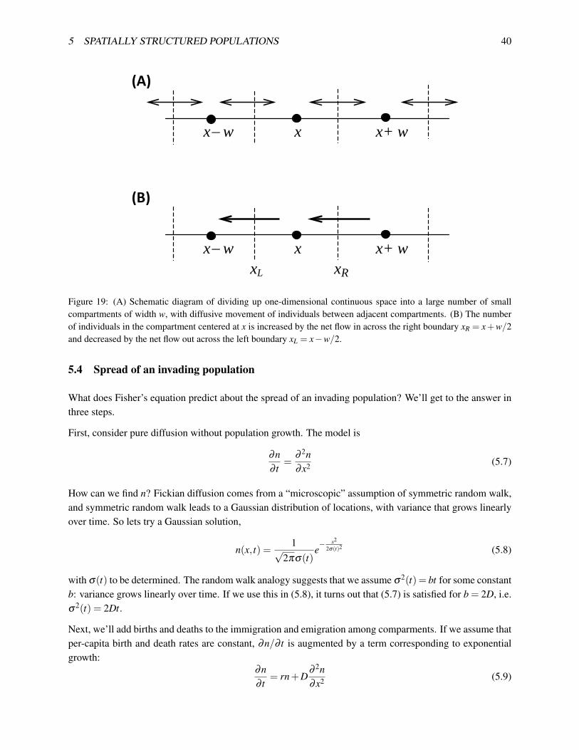
5 SPATIALLY STRUCTURED POPULATIONS 40
(A) x− w x x+ w (B) x− w x x+ w xL xR Figure 19: (A) Schematic diagram of dividing up one-dimensional continuous space into a large number of small
compartments of width w, with diffusive movement of individuals between adjacent compartments. (B) The numberof individuals in the compartment centered at x is increased by the net flow in across the right boundary xR = x+w/2and decreased by the net flow out across the left boundary xL = x−w/2.
5.4 Spread of an invading population
What does Fisher’s equation predict about the spread of an invading population? We’ll get to the answer inthree steps.
First, consider pure diffusion without population growth. The model is
∂n∂ t
=∂ 2n∂x2 (5.7)
How can we find n? Fickian diffusion comes from a “microscopic” assumption of symmetric random walk,and symmetric random walk leads to a Gaussian distribution of locations, with variance that grows linearlyover time. So lets try a Gaussian solution,
n(x, t) =1√
2πσ(t)e− x2
2σ(t)2 (5.8)
with σ(t) to be determined. The random walk analogy suggests that we assume σ2(t) = bt for some constantb: variance grows linearly over time. If we use this in (5.8), it turns out that (5.7) is satisfied for b = 2D, i.e.σ2(t) = 2Dt.
Next, we’ll add births and deaths to the immigration and emigration among comparments. If we assume thatper-capita birth and death rates are constant, ∂n/∂ t is augmented by a term corresponding to exponentialgrowth:
∂n∂ t
= rn+D∂ 2n∂x2 (5.9)

5 SPATIALLY STRUCTURED POPULATIONS 41
If we set u(x, t) = e−rtn(x, t), we find that u obeys (5.7) So the solution of (5.9) for a unit point release atx = 0, t = 0 is
n(x, t) =n0ert
2t√
πDe−x2/4Dt . (5.10)
How fast does this population spread? A Gaussian distribution has infinite (but thin) tails. The usual way ofdefining population spread rate is to ask, at what spatial location xc does n(x, t) falls below some thresholdvalue nc? Setting n(xc, t) = nc and solving, gives a mess that can be expressed as:
xc = 2t
√rD+O
(1t
log(√
t)).
So the radius of occupied territory grows linearly with time, at rate c = 2√
rD. This is, as Skellam pointedout, the key prediction that is supported by the data on muskrat spread.
5.5 Fisher’s equation
Finally, we now add density-dependent population growth using the logistic model, bringing us back toFisher’s equation,
∂n∂ t
= rn(1−n/K)+D∂ 2n∂x2 (5.11)
We look for traveling wave solutions to this equation, illustrated in Figure 20. As the wave front advances,populations far behind the front converge to carrying capacity. The speed of the wave is the distance that thewave front advances from one generation to the next.
By methods FAR beyond this class, it can be shown that Fisher’s equation has traveling wave solutions withconstant speed c for all c≥ 2
√rD. However, if the initial population is limited to a finite area, the population
converges to spreading in a wave at the slowest speed, exactly the same speed as with exponential growth.
What this says “physically” is that the wave front is “pulled” by the leading edge of the invasion, rather than“pushed” by the population far behind the leading edge. Behind the leading edge, where population densityis high, the exponential and logistic models behave very differently from each other. But near the edge of thewave, population density is low, and rn(1−n/K)≈ rn so they act the same. Because the furthest-out-frontindividuals drive the expansion, the rate of population spread is the same for the logistic and exponentialgrowth models.
Note: the one-dimensional model also predicts the asymptotic spread rate in two dimensions. Why: asthe population has spread out from the source, the boundary of the occupied area (an expanding circle)becomes less and less curved: nearly straight. Consider what’s happening at (x,0),x� 0. The boundaryof the occupied area is nearly straight, so to a good approximation we have n(x,y, t) = n(x, t) — no ydependence. Then the 2-dimensional diffusion equation collapses to the one-dimensional equation, so thepredicted spread rate is the same.
5.6 Theory meets data
The prediction c = 2√
rD means that rates of spread can be predicted from experimental data on populationgrowth and individual movements. For a point release without population growth, we found σ2(t) = 2Dt.

5 SPATIALLY STRUCTURED POPULATIONS 42162 MARK KOT
-0 0.2 0.4 0.6 0.8 10.0
0.5
1.0Model 1
-0 1 2 30.0
0.5
1.0Model 2
-0 1 2 30.0
0.5
1.0Model 3
-0 5 10 15 200.0
0.5
1.0Model 4
-0 0.5 1 1.5 20.0
0.5
1.0Model 7
Space (km)
-2-
Popu
latio
n D
ensi
ty
FIGURE 10: Iterated integrodifference equations. Five integrodifferenceequations were constructed by combining the Beverton-Holt recruitmentcurve, for R0 = 10, with each of the dispersal kernels in Figure 9. Eachequation was iterated for 12 generations starting with an initial pointsource of strength n0 = 50/32767 centered at the origin. We integratedusing a FFT-assisted implementation of the extended trapezoidal ruleon a domain of length 50 with 32768 grid points. The solutions formodels 1, 2, 3, and 7 rapidly converged to constant-speed travelingwaves. In contrast, the solution for model 4 continued to accelerate.
Figure 20: Examples of traveling wave solutions for a population started from a few individuals near x = 0. Thefigures show population spread over 12 generations, for different movement distributions fitted to the same data set onmovements by emphDrosophila melanogaster, with the same model for local population growth. From Kot (2003).
Table 1: Comparison of observed rates of invasive species spread with predictions from simple diffusion models (FromShigesada and Kawasaki 1997)
Species Predicted rate km/yr, 2√
rD Observed spread rateMuskrat 6-32 1-25Sea otter: northward 1.7 1.4Sea otter: southward 3.5 3.1Black death 720 320-650Rabies in fox 70 30-60Cabbage butterfly (N. America) ≤ 90 15-170Gypsy moth (US) ≤ 2.5 3-20Cereal leaf beetle 1.7 27-90
So if we measure time in generations, D is half the mean-square displacement between parents (t = 0) andoffspring (t = 1), and r = logλ , where λ is the per-generation finite rate of increase.
Sometimes the prediction works pretty well, and other times it fails spectacularly (Table 5.6). Anotherproblem is that rate of increase in the square-root of occupied area is not always linear. It can be accelerating,or biphasic (SLIDES from Shigesada and Kawasaki).
A key problem with simple diffusion models is that displacement distributions are often leptokurtic or “fat

5 SPATIALLY STRUCTURED POPULATIONS 43158 MARK KOT
-0
0.1
0.2
0.3
0 20 40 60 80 100Distance (m)
-0
0.1
0.2
0.3
0.4
0 50 100 150 200Distance (m)
Rel
ativ
e Fr
eque
ncy
Rel
ativ
e Fr
eque
ncy
FIGURE 6: Frequency distributions of distances (top) for the dispersalof 127,070 seeds of the European ash (Fraxinus excelsior) (Geiger, 1971)and (bottom) between natal sites and nests of the 53 queens of the paperwasp Polistes riparius (Makino et al., 1987). Note the wide tails.
INTEGRODIFFERENCE EQUATIONS 159
-0
0.05
0.1
0.15
0.2
0 20 40 60 80 100 100Distance (m)
-0
0.05
0.1
0.15
0 10 20 30 40Distance (cm)
Rel
ativ
e Fr
eque
ncy
Rel
ativ
e Fr
eque
ncy
FIGURE 7: Frequency distributions of distances (top) for the dispersalof 74 black walnuts (Juglans nigra) (Stapanian and Smith, 1978) and(bottom) for the dispersal of 246 seeds of Vulpia fasciculata (Carey andWatkinson, 1993). The modal dispersal distances are positive.
Figure 21: Examples of leptokurtic dispersal distributions, from Kot (2003)
tailed” (Figure 21). The name leptokurtic comes from the statistical measure called kurtosis
κ =µ4
µ22
where µk is the kth central moment of the distribution. For movement distributions, µk means: raise allmovement distances to the kth power, and compute the mean of those values. The denominator in κ is thesame as the variance of the distribution squared. A Gaussian distribution has κ = 3. A distribution withκ > 3 is called leptokurtic or fat-tailed. Warning: Some call κ − 3 the kurtosis , and some only call adistribution fat-tailed if its tails decrease slower than exponentially.
Much recent research on population spread and redistribution is therefore concerned with the causes andconsequences of leptokurtic dispersal.
5.7 Fat-tailed dispersal: integrodifference models
The most important consequence of fat tails is that they can explain faster-than-Fisher rates of spread. Onepopular approach uses discrete-time analogs of Fisher’s equation, which can have non-Gaussian dispersaldistributions. The model assumes that the organism’s life cycle involves alternative phases of local demog-raphy (births and deaths) without movement, and movement without births or deaths.

5 SPATIALLY STRUCTURED POPULATIONS 44
The state of the population is still n(x, t), the population density at location x at time t. The first thingthat happens in each time step is local population growth. So at each location y, the population densitychanges from n(y, t) to f (n(y, t)) representing the net effect of births and deaths, which can depend on localpopulation density (e.g., higher mortality at crowded locations). The next step is movement. Again, Letk(d) be the probability distribution of dispersal distances (d > 0 is move right, d < 0 is move left). As inFigure (21) it is generally the case that most individuals don’t go far, but a few do.
To find the population density n(x, t + 1) after movement, we just need to add up all the ways that anindividual can have gotten to location x at a given time: they started at some location y (either as newbornsor surviving older individuals), and moved to location x. So the model is
n(x, t +1) =∫
k(x− y) f (n(y, t))dt (5.12)
Kot et al. (1996) analyzed this model to determine the long-term rate of population spread that it predicts.
• If k(d) is Gaussian, the asymptotic wave speed is exactly the same as Fisher’s equation, if we identifyr = log f ′(0),2D = variance of the dispersal distribution k(d).
• if k(d) is fat-tailed, the asymptotic wave speed is faster than the Fisher equation prediction based on rand the variance of the dispersal distribution.
• if k(d) is very fat-tailed, instead of there being an asymptotic wave speed, the rate of populationspread is constantly accelerating. “Very fat tailed” means that the tail of the distribution decreasesslower than exponentially, for example k(d) ∝ 1/(1+ cd2).
The “moral” of these results is that populations spread by extremes. The tail of the dispersal distribution – therare individual who goes an exceptionally great distance – determines how fast population spread occurs.The typical movement behavior of a typical individual can be completely misleading when the dispersaldistribution is fat-tailed. The two observations about population spread that are problematic for diffusionmodels - spread much faster than predicted, and accelerating waves of spread - are both exmplained by theempirical observation of fat-tailed dispersal distributions.
Example: Clark (1998) specifically considered Reid’s paradox of tree returns after the last glaciation. Al-lowing 5% of red maple seeds to follow a very fat-tailed distribution compatible with the data on seeddispersal, gave rise to a rapidly accelerating wave of spread and a 10-fold increase in spread rate within 100years, relative to the spread rate without a fat tail.
5.8 What causes fat-tailed dispersal distributions?
In some cases fat-tailed dispersal distributions can just be the result of physical processes, such as thepassively-dispersed seeds of many plants (Figure 21).
For wind-dispersed seeds, understanding seed dispersal is done through detailed physical modeling of seedsblown by wind. The distribution of dispersal distances depends on the local wind patterns, on the ballisticsof the seed, and on how hard the seeds are attached to the parent. A loosely attached seed (think: dandelion)

5 SPATIALLY STRUCTURED POPULATIONS 45
will blow off in a mild wind. A tightly attached seed will only go when the winds are stronger. Variabilityin attachment strength allows a parent plant to have some seeds that are likely to fall nearby, others that arelikely to go further.
In many cases, fat tails are the result of there being multiple distinct modes of dispersal: different sub-populations moving by different mechanisms, or according to different “rules”.
SLIDES: multiple modes of seed dispersal on animals. A seed that can attach itself to any passing mammalwill attach to some that move far and some that don’t.
One measure of “fat tails” is kurtosis: the ratio of the fourth central moment to the square of the secondcentral moment (which is the variance). The Gaussian distribution has kurtosis=3. But if you mix twoGaussian distributions with different variances, you get a fat-tailed distribution (kurtosis > 3). For example:
> z1=rnorm(5000); mean(z1^4)/(var(z1)^2);
[1] 3.035456
> z2=c(rnorm(4000,sd=1),rnorm(1000,sd=4)); mean(z2^4)/(var(z2)^2);
[1] 9.596698
So even if seeds on sheep have a Gaussian dispersal distribution, and seeds on goats have a Gaussian dis-persal distribution, the dispersal distribution for all seeds combined will be fat-tailed.
For animal movements, multiple dispersal modes are the outcome of individual decisions: do I stay hereor move on? Turn right or turn left? The idea that this leads to multiple dispersal modes forced itself onpeople when attempts were made to “scale up” from short-term studies of individual movement to long-termpatterns of population spread, and discovered that it often didn’t work.
It is now common for animal movement data to be decomposed into different movement “modes”. Moraleset al. (2004) analyzed data on movements of elk released in east-central Ontario, Canada. Their analysissupported the existence of two modes of movement behavior. Elk are either in an “encamped” state inwhich daily movements are small and turning angles are high (so there are many changes in the direction ofmovement), or in an “exploratory” state in which daily movements are several kilometers and turning anglesare small.
Subsequent work has looked at later stages of this re-introduced population, including herd movements(when individuals are influenced by other animals), and movement within home ranges where short-scalelocal movements alternate with occasional large moves (e.g., Fryxell et al. 2008). But the big picture isalways the same: individuals having different modes of movement, with changes between them influencedby what they are experiencing and have experienced in the past (e.g., elk like to re-visit places that they’vevisited before within their home ranges).
So, reiterating what may be this course’s overarching theme: ecosystems are collections of individualsmaking informed decisions (and even plants make informed decisions!). As a result, the most generalprinciple for understanding ecological systems is Darwinism, constrained by physics and history.

5 SPATIALLY STRUCTURED POPULATIONS 46
5.9 References
M.J. Eaton, P.T. Hughes, J.E. Hines and J.D. Nichols. 2014. Testing metapopulation concepts: effects ofpatch characteristics and neighborhood occupancy on the dynamics of an endangered lagomorph. Oikos123: 662676.
Fryxell, JM, M Hazell, L Borger, BD Dalziel, DT Haydon, JM Morales, T McIntosh, RC Rosatte. 2008.Multiple movement modes by large herbivores at multiple spatiotemporal scales. PNAS USA 105: 19114-19119.
Gilbert-Norton, L., R. Wilson, J.R. Stevens and K.H. Beard. 2010. A meta-analytic review of corridoreffectiveness. Conservation Biology 24: 660-668.
Hanski, I. 1994. A practical model of metapopulation dynamics. Journal of Animal Ecology 63: 151-162.
Hanski, I., A. Moilanen, T. Pakkala and M. Kuussaari. 1996. The quantitative Incidence Function modeland persistence of an endangered butterfly metapopulation. Conservation Biology 10: 578-590.
Hanski, I.A. and M. Gilpin (eds.) 1997. Metapopulation Biology. Academic Press, NY.
Hanski, I.A. and O.E. Gaggioti (eds.) 2004. Ecology, Genetics and Evolution of Metapopulations. Aca-demic Press, NY.
Kot, M., M.A. Lewis, and P. van den Driessche. 1996. Dispersal data and the spread of invading organisms.Ecology 77: 2027-2042.
Kot, M. 2003. Do invading organisms do the wave? Canadian Applied Mathematics Quarterly 10: 139-170.
M. P. Kreuzer and N. J. Huntly. 2003. Habitat-specific demography: evidence for source-sink populationstructure in a mammal, the pika. Oecologia 134: 343-349.
Levins, R. 1969. Some demographic and evolutionary consequences of spatial heterogeneity for biologicalcontrol. Bulletin of the Entomological Society of America 15: 237-240.
Lidicker, W. Z. 1975. The role of dispersal in the demography of small mammals. Pages 103- 128 in F.B. Golley, K. Petrusewicz, and L. Ryszkowski (eds.). Small Mammals: Their Productivity and PopulationDynamics. Cambridge University Press, Cambridge, United Kingdom.
Morales, J.M. and S.P. Ellner. 2000. Scaling up animal movements in heterogeneous landscapes: theimportance of behavior. Ecology 83: 2240-2247.
Morales, J.M., D.T. Haydon, J. Frair, K.E. Holsinger, J.M.Fryxell. 2004. Extracting More out of RelocationData: Building Movement Models as Mixtures of Random Walks. Ecology 85: 2436-2445.
Okubo, A. and S.A. Levin. 2001. Diffusion and Ecological Problems: Modern Perspectives (2nd edition).Springer, New York.
Ozgul, A. et al. 2006. Effects of patch quality and network structure on patch occupancy dynamics of ayellow-bellied marmot metapopulation. Journal of Animal Ecology 75: 191202.
Pulliam, H. R. 1988. Sources, sinks, and population regulation. American Naturalist 132:652- 661

5 SPATIALLY STRUCTURED POPULATIONS 47
Shigesada, N., K. Kawasaki and Y. Takeda. 1995. Modeling stratified diffusion in biological invasions.American Naturalist 146: 229-251.
Shigesada, N. and K. Kawasaki. 1997. Biological Invasions: Theory and Practice. Oxford University Press,Oxford UK.
Shmida, A. and S. Ellner. 1984. Coexistence of plant species with similar niches. Vegetatio 58: 29-55.
Tewksbury, J.J. et al. 2002. Corridors affect plants, animals, and their interactions in fragmented landscapes.PNAS 99: 12923 - 12926.
Tilman, D. and P. Kareiva (eds.) 1997. Spatial Ecology: The role of Space in Population Dynamics andInterspecific Interactions. Princeton University Press, Princeton NJ.

6 EXPLAINING BIODIVERSITY 48
6 Explaining biodiversity
What factors control species richness, and why? This is one of ecology’s classic and most basic questions.Attempts to answer it began over a century ago, but I approach it here from a modern perspective. Myfocus is going to be on alpha-diversity: explaining how numerous species can coexist within one habitat,and why some habitats support more species than others. My focus will be on the challenge to our under-standing posed by hyper-diverse communities, because these challenge our intuitive idea that species coexistbecause they have “different niches”. Looking at extreme cases is often useful when basic questions are stillunanswered, and as we’ll see, the question of what forces maintain biodiversity is still unanswered.
• The issues raised by coexistence of many similar species was brought into sharp focus by Hutchinson’s“Paradox of the plankton” (1961)
“The problem that is presented by the phytoplankton is essentially how it is possible for anumber of species to coexist in a relatively isotropic or unstructured environment all com-peting for the same sorts of materials. The problem is particularly acute because there isadequate evidence from enrichment experiments that natural waters, at least in the sum-mer, present an environment of striking nutrient deficiency, so that competition is likely tobe extremely severe. According to the principle of competitive exclusion (Hardin, 1960)known by many names and developed over a long period of time by many investigators(see Rand, 1952; Udvardy, 1959; and Hardin, 1960, for historic reviews), we should ex-pect that one species alone would outcompete all the others so that in a final equilibriumsituation the assemblage would reduce to a population of a single species.”
As an example, Hutchinson (1961) presented data on some Scandinavian lakes with over 30 speciesof diatoms. Diatoms have high requirements for silicon, which creates a niche difference betweendiatoms and other phytoplankton. This can explain coexistence of diatoms with other phytoplankton− but how can there be 30 stably coexisting species of diatoms?
• Tropical rain forests: Wright (2002) SLIDE: “Plant alpha diversity reaches astonishing levels in equa-torial forests. For example, a single hectare of Amazonian forest can support more than 280 treespecies with diameter at breast height (d.b.h.) ≥ 10 cm (Valencia et al. 1994; Oliveira and Mori1999). Tree diversity is equally remarkable at slightly larger spatial scales. A 0.52-km2 plot in Bor-neo and a 0.25-km2 plot in Ecuador support 1,175 and 1,104 tree species with diameter at breast height(d.b.h.) ≥ .1 cm, respectively (LaFrankie 1996; R Condit, personal communication). In contrast, the4.2×106 km2 of temperate forests that cover Europe, North America and Asia support just 1,166 treespecies with maximum height > 7m (Latham and Ricklefs 1993).” The Cornell Ag Quad is about0.65 hectares. How can 280 different tree species coexist in less than twice that much area?
• Herbaceous plants. SLIDE: longleaf pine savanna (Myers and Harms 2009) formerly covered over370,000 km2 in the Southeastern US. Savanna is maintained by lightning-started fires that typicallyoccurred 1 or more times per decade. α−diversity of forbs, grasses and shrubs: ≈ 30 species in 1 m2,103 species in 100m2. Deborah Goldberg (University of Michigan) has sampled sites with 60 or moreherbaceous species in one square meter (personal communication).

6 EXPLAINING BIODIVERSITY 49
Coexistence of primary producers (plants, algae) has been a major focus in general. If you have 60 herba-ceous plant species, it’s no trouble to “explain” hundreds of herbivores or even more: each plant supportingseveral specialists that use different parts of the plant, plus many possible generalists that each utilize adifferent group of plants. So: 60 plant species in 1 square meter; over 280 tree species in one hectare (theAg Quad is about 1.5 hectares); and over 1000 plant species in 500m × 500m. How is that possible?
6.1 Stabilizing vs. equalizing mechanisms
Not surprisingly, many different ideas have been proposed. One useful way to think about different coex-istence mechanisms, introduced by Peter Chesson, is by distinguishing between stabilizing and equalizingmechanisms. I will explain these using a model for competing plant speces, introduced by A.R. Watkinsonin the 1970’s.
The Watkinson model is a lot like the two-species Lotka-Volterra model (Mittelbach Ch.7, pages 126-131).As Mittelbach notes (p. 131) Lotka-Volterra models “have severe limitations when applied to natural com-munities” but Watkinson’s model actually does pretty well at modeling some systems (especially herbaceousplants). The model starts with exponential growth of both species, in discrete time:
N1(t +1) = λ1N1(t), N2(t +1) = λ2N2(t).
Then, the growth of each species is reduced by competition, both within and between species. The strengthof competition is determined by the competition coefficients ai j, which measure the direct effect of speciesj on the population growth of species i. The model is
N1(t +1) =λ1N1(t)
1+a11N1(t)+a12N2(t)
N2(t +1) =λ2N2(t)
1+a21N1(t)+a22N2(t)
(6.1)
The parameters λ1,λ2 and the competition coefficients can be measured experimentally. Mittelbach (2012)has a good, detailed discussion about the experimental methods and some examples of studies that haveused them.
We now want to ask: under what conditions can the two species coexist? In section 8.2, analysis of themodel shows that the two species will persist if
a21
a11<
λ2−1λ1−1
<a22
a12. (6.2)
The way to think about this, is that we want the leftmost expression to be small, and the rightmost to belarge, for coexistence to occur. That is:
a11 > a21, a22 > a12. (6.3)
“I” affect “myself” (the same species) more than “I” affect “you” (the other species).
A stabilizing mechanism is anything that leads to (6.3). It leads to stable coexistence because each speciesis pushed away from extinction. When “I” am rare, “I” see a world full of individuals that don’t compete

6 EXPLAINING BIODIVERSITY 50
with “me” very much. “You” (the other species), on the other hand, have a lot of competitors (others likeyou). Therefore “I” have an advantage, and my frequency in the community tends to increase.
An equalizing mechanism is something that reduces the difference between λ1 and λ2, so that
λ2−1λ1−1
is neither very small or very large. That makes it easier for the competition coefficients to satisfy thecondition for coexistence. If λ1 ≈ λ2, then the differences in (6.3) can be small, and coexistence will stilloccur.
A useful approximation is that the population growth rate of species 2 when it is at low frequency in thecommunity is approximately 1 plus
(λ2−λ1)+
(1− a21
a11
)λ1 (6.4)
Species 2 can increase if the expression is positive. The first term on the right is intrinsic fitness differencebetween the species, because λ is the population growth rate in the absence of competition. The secondterm is a “boost” due to interspecific competition being weak relative to intraspecific competition.
Chesson (2000) notes that similar approximations hold for many models of interspecific competition, in-cluding models with many species. What you get is something like (for species i)
(λi− λ )+(1−ρ)D (6.5)
where λ is the mean fitness of competitors, D > 0 is a constant, and ρ is a measure of interspecific vs.intraspecific competition. The second term is positive so long as interspecific competition is weaker thanintraspecific competition (so ρ < 1). The first term has to be negative for some of the species: it isn’tpossible for all of them to be above average. So in order for all the species to coexist, the second term hasto be larger in magnitude than the first term, for all of the species. A stabilizing mechanism is somethingthat makes the second term large (i.e., it makes ρ small because intraspecific competition is weaker thaninterspecific competition). An equalizing mechanism is something that makes the first term small.
6.2 Niche differentiation
How does stabilization happen, mechanistically? The classical answer is niche differences. The original(Grinell) definition of niche was in terms of trophic relations: who eats whom. If “you” and “I” eat differentthings, then more of “me” won’t keep you from getting what you need, and vice-versa.
Classic example: MacArthur’s warblers (SLIDE) differing in foraging locations within trees.
SLIDE: theoretical resource utilization curves (Resource on x-axis, Utilization on y-axis).
SLIDE: based on his warbler work, MacArthur related bird species diversity to foliage diversity. The idea is:the wider the range of variation there is along some “niche axis” the more species will fit into it. MacArthurand MacArthur (1961) calculated bird species diversity in different sites (using the Shannon-Weaver index∑i
pi log(pi)), with the Foliage Height Diversity, the same index with pi being the fraction of foliage at height
i.

6 EXPLAINING BIODIVERSITY 51
SLIDE: Multidimensional niche space. Hutchinson’s definition of niche was the region of resources it canuse, in a multidimensional space of “niche axes”. Axes can include things like time of day, temperature,season of the year, etc. as well as which resources are used – so it can go further than Grinell in explaininghigh species richness.
LOTS of early (1960-1980) theory about species richness was based on the image of species dividing upa multidimensional “niche space”. In these theories, community structure is the result of species invading,competing, and evolving their resource use curves. A buzzword for this body of work is species packing.This approach ’ But “species packing” has trouble explaining 30-60 herbaceous species in one square meter,and 1000 tree species in 0.25 km2 of tropical forests, because all plants need the same basic things: light,water, basic mineral nutrients, and a place to grow.
SLIDE: Grubb quote. “Although many different factors are involved in the full definition of an ani-mal’s niche, one can fairly readily imagine sufficient niches for all the animal species known, using food-requirements alone; the million or so animal species can easily be explained in terms of the 300,000 speciesof plants (so many of which have markedly different parts such as leaves, bark, wood, roots, etc.) and theexistence of three to four tiers of carnivores (Hutchinson, 1959). There is no comparable explanation forautotrophic plants; they all need light, carbon dioxide, water and the same mineral nutrients.”
So something more subtle must be going on.
6.3 Resource competition
SLIDE: using the same resource, in different ways. Two plant species both need N and P, but one uses Nvery efficiently (so it doesn’t need very much), and the other uses P very efficiently (so it doesn’t need verymuch).
Resource competition theory requires mechanistic models. There’s no way, really, to look at the resourceuse curves and calculate competition coefficients ai j. We really have to model how species consume andutilize resources. This material is covered in Mittelbach, pp. 132-142, and 150-154.
To start simple, consider two species whose population growth rates are both limited by one resource that isin short supply, all other resources being abundant. The simplest model assumes that
• Resource is supplied at a constant rate R0, and is consumed by the two species.
• Each species has a per-capita birth rate proportional to the per-capita rate of resource uptake, and aconstant death rate.
That gives us:dR/dt = R0− f2(R)n1− f2(R)n2
dn1/dt = χ1 f1(R)n1−d1n1
dn2/dt = χ2 f2(R)n2−d2n2
(6.6)
Here d1,d2 are the per-capita death rates of the species, f1, f2 are their per-capita rates of nutrient uptake, andχ1,χ2 are the conversion rates between nutrient uptake and offspring production. The limiting is supplied

6 EXPLAINING BIODIVERSITY 52
at rate R0. This model is well-mixed – we don’t take account of spatial variability in resource availability orthe density of the two species.
Can both species coexist? The answer is no. Imagine the system going to steady state, with both speciescoexisting. Then there is some resource abundance R∗ at the steady state, and we must have
χ1 f1(R∗) = d1, χ2 f2(R∗) = d2,
an enormous coincidence. Not only must the two functions χi f I(R)−di cross, they have to cross at exactlythe value of R that the system reaches at steady-state.
The basic result for the simple two-species, one-nutrient model is that you always have competitive exclusion(Smith and Waltman 1995):
Let R∗1,R∗2 be the nutrient levels at which each species can just barely survive (χi fi(R∗i ) = di).
Then whichever species has the lower R∗ drives the other to extinction.
SLIDE: Mittelbach Fig 8.1, two diatoms competing for limiting Phophorus. Growing them separately,Asterionella has the lower R∗ by a small amount, so it is predicted to win in competition, and it does.Similarly, Tilman, Matson, and Langer (1981) measured the R∗’s for silica of the diatoms Asterionellaformosa and Synedra Ulna. This time Synedra had the lower R∗, and it out-competed Asterionella.
Note the audacity of these experiments. You grow each species in isolation and then predict what willhappen when you put them together. And then, it actually happens.
6.3.1 Two resources
Since one resource allows only one competitor to persist, coexistence of competitors must involve severallimiting resources. Suppose there are two, which I’ll call N and P, and each species’ growth rate is limitedjointly by N and P. The simplest situation is when each nutrient is essential, in the sense that species i canpersist if N ≥ N∗i and P≥ P∗i . But if either N < N∗i or P < P∗i , then species i has a birth rate that is too lowto make up for its death rate, and it dies out.
Part of the outcome is easy to guess. If species 1 needs less N and less P than species 2, it wins (i.e.,N∗1 < N∗2 ,P
∗1 < P∗2 ). The other way around, species 2 wins.
But if one needs less N to get by, and the other needs less P, then coexistence is possible. Whether or notthis happens turns out to depend on two things: how fast each species consumes each resource, and the rateof supply for each resource. The details get complicated, going into them is not the best use of our time.See pp. 132-142 in Mittelbach if you’re interested. The key result is that whether coexistence occurs (ratherthan one species out-competing the other) depends on the relative rates at which N and P are supplied to thesystem. For example, suppose that much more N is supplied than P. Then both species will be stop growingwhen they run out of P (and N will still be available in excess), so the one with the lower P∗ will win. WithP available in excess, the one with the lower N∗ will win. Somewhere in the middle, the species might beable to coexist.
Tilman (1982) reports good results for predictions of coexistence versus exclusion in systems with morethan one limiting nutrient. Rothaupt (1988) tested the theory using two species of rotifers feeding on two

7 REGENERATION NICHE AND SPACE-DEPENDENT MECHANISMS 53
species of algae, varying the relative availability of the food and the “natural” mortality rate of the predators(chemostat dilution rate).
SLIDE: Mittelbach Fig. 7.3, growth rates of the two rotifer species, on the two algal species, as a functionof algal abundance.
SLIDE: Outcome of experiments with the two species grown together (from Rothaupt 1988)
Dybzinski and Tilman (2007) report results from an 11 year competition experiment with nitrate and lightas the two limiting resources. Their findings were both good and bad for resource competition theory:
consistent with the predictions of resource competition theory, the resource requirements ofindividual species determine the long-term outcomes of interspecific interactions. However,only two of our eight competition pairings resulted in coexistence, and it was unclear whethertheir coexistence was because of an N-light trade-off. Thus, while competition for multipleresources might maintain some diversity in natural communities, other mechanisms are almostcertainly operating to maintain the remainder.
Mittelbach (2012, pp. 153) has some excellent remarks on testing theory in ecology. Resource competitiontheory proved to be logically sound. It was supported by experiments that were set up to satisfy the theory’sassumptions, and then carried out to see if the theory’s predictions came true – which is most often did. Butin the field, it now seems that the conditions leading to coexistence don’t often enough for it to be a majorfactor in maintaining species richness in plant communities.
An important complication to the theory above is that we have assumed that coexistence occurs at a steadystate. In our simple model above, that’s the only possibility (Smith and Waltman 1995) and we get com-petitive exclusion. But a different model for R can change that. If we replace the constant supply rate R0by bR(1−R/K), then we have a predator-prey model (i.e. R is an organism, not a nutrient) and we can getcycles. The result is that two species feeding on R may be able to coexist.
7 Regeneration niche and space-dependent mechanisms
Grubb (1977) argued that the established plant is the wrong place to look for niche differences, because theirrequirements for survival and growth really are very similar. The important differences are in the conditionsthat are required for making seeds, and in the seeds’ requirements for successful establishment.
SLIDE: BCI trees and seeds.
Grubb (1977) emphasized seed production and seed germination, and how those vary in time and space.When Grubb wrote, there wasn’t much information available on temporal variability, but 20 years later therewas a lot (SLIDE: Hairston 1996 table). Grubb was able to cite studies on the conditions required for seedgermination. Those differ greatly among species, and he suggested that those would lead to separation ofspecies in space or time.
Grubb (1977) has been enormously influential. Since then, theories for biodiversity focus on the process ofone individual dieing and being replaced by another. The mechanism for coexistence is that for some reason

7 REGENERATION NICHE AND SPACE-DEPENDENT MECHANISMS 54
two species regenerate in different places or at different times. We’ll consider the first idea first.
Competition-colonization tradeoff . Several related hypothesis focus on species coexisting by usingspace in in different ways. A Competitor species is good at keeping space that it now occupies; a Colonizeris better at getting first to open space created by disturbance. Example: early and late successional treespecies, dividing up space according to time since last disturbance. But it can also be more subtle: twoannual plants, one of which has very widely dispersed seeds, the other has big, highly competitive seedsthat stay near their parent. Many studies have examined how interspecific variation in seed size leads tocompetition-colonization tradeoffs, and asking how important it is for coexistence.
SLIDE: tropical trees have a tradeoff between ability to grow in gaps (colonizer) and ability to survive inshade (competitor).
Reciprocal replacement/Janzen-Connell Hypothesis . Originally formulated for tropical trees, this hy-pothesis asserts that each tree attracts specialist natural enemies (pathogens, herbivores, etc.) so that itsown seedlings cannot establish near their parent. If one species becomes too abundant, it then has very lowrecruitment, so no single species can monopolizing space.
• According to Wright (2002), most studies looking for Janzen-Connell in tropical forests have foundit. That has continued to be true. Metz et al. (2010) looked as seedling survival of 163 tree speciesin Yasuni National Park, Ecuador, “an ever-wet, hyper-diverse lowland Amazonian rain forest”, andfound that seedlings survived better if they are surrounded by distantly-related trees.
• It also occurs in temperate forests. Kerry Woods (a student of Robert Whittaker at Cornell) com-pared mortality of beech and maple seedlings under beech and maple canopy trees. He found thatbeech saplings (1-4m height) had higher mortality under beech trees, and maple saplings had highermortality under maple trees (Woods 1979).
Johnson et al. (2012) used the US Forest Service’s Forest Inventory and Analysis database, whichincludes 151 species from more than 200,000 forest plots. They analyzed relationships between treeabundance and seedling abundance, within fully forested plots (circes of area of 168.33 m2). Theyfound that seedling abundance was negatively affected by the abundance of conspecific trees, but notby the abundance of heterospecific trees. They also found that stronger intraspecific density depen-dence was associated with higher tree species richness (SLIDE). This matches exactly our analysis ofstabilizing mechanisms: if each aii is big, it’s easy for species to coexist.
• Petermann et al. (2008) showed that Janzen-Connell effects are widespread and strong in grasslands,and that the mechanism is buildup of soil-borne pathogens that reduce the competitive ability ofspecies on soils that they have occupied. SLIDE: When grown in competition with other species, 23out of 24 species tested had lower biomass growing on “home” soils (where the same species hadgrown before) than on “away” soils, and the average biomass reduction was about 50%. When grownin competition with conspecifics, the biomass reduction was about 30% on average.
Petermann et al. (2008) found that treating the soil with fungicide did not eliminate the home-awaydifference: complete sterilization was required. However, in a similar experiment using seedlings of

7 REGENERATION NICHE AND SPACE-DEPENDENT MECHANISMS 55
VARIAT ION WITH LAT ITUDINAL AND PRECIP ITAT ION
GRADIENTS
We found no significant effect of absolute latitude on effect size(QM = 1.69, d.f. = 1, P = 0.194; Fig. 5a). Similarly, there wasno significant difference between studies located in the tropicsversus studies from the temperate zone (QM = 0.064, d.f. = 1,P = 0.8). Even when comparing studies within a single region(possible only for studies from the Americas and Asia), wefound no significant difference between tropical and temperatestudies in the Americas (QM = 1.858, d.f. = 1, P = 0.173;Fig. 2) or Asia (QM = 0.114, d.f. = 1, P = 0.735; Fig. 2), and
no significant correlation of effect size with latitude withinthese two regions (America: QM = 1.081, d.f. = 1, P = 0.298;Asia: QM = 1.421, d.f. = 1, P = 0.233).We found a marginally significant correlation of effect size
with overall precipitation (slope = �0.24 � 0.12, QM = 3.698,d.f. = 1, P = 0.054; Fig. 5b). When we examined tropical andtemperate studies separately, the correlation was significant inboth cases (tropical: slope = �0.32 � 0.16, QM = 4.08, d.f. =1, P = 0.04; temperate: slope = �1.02 � 0.45, QM = 5.05,d.f. = 1, P = 0.02; Fig. 5b).
VARIAT ION AMONG REGIONS AND STUDY SITES
Of the four regions, only America and Asia had significantlynegative effect sizes (overall model with all four regions test-ing difference of effect size from zero: QM = 16.284, d.f. =3, P = 0.003; Fig. 2). There was no significant differenceamong regions in their effect sizes (QM = 4.13, d.f. = 3,P = 0.25). However, there were relatively few tests from Eur-ope and Africa.There was no significant difference in effect size for studies
from BCI, Panama (n = 14), compared to all other studies(QM = 1.27, d.f. = 1, P = 0.26) or all other tropical studies(QM = 1.73, d.f. = 1, P = 0.19). Likewise, there was no sig-nificant difference in effect size for studies from CochaCashu, Peru (n = 16), compared to all other studies(QM = 0.05, d.f. = 1, P = 0.82) or all other tropical studies(QM = 0.03, d.f. = 1, P = 0.87).
VARIAT ION AMONG LIFE-H ISTORY STAGES
We found a significant difference between life-history stagesin effect size (QM = 6.192, d.f. = 1, P = 0.013; Fig. 2). Seed-lings showed a significantly lower odds ratio than seeds(seedlings: log OR = �0.78 � 0.19; seeds: log OR =�0.17 � 0.16), indicating stronger negative effects of conspe-cific density and proximity at the seedling stage. In fact, whenthe two life stages were tested separately, significant negativeeffects of conspecific density and proximity were only found
−2.0 −1.0 0.0 0.5 1.0Effect Size (ln[OR])
Cat
egor
y
distance and density studies (154)
distance studies only (120)
density studies only (34)
temperate (59)tropical (95)
temperate America (33)tropical America (61)
temperate Asia (19)tropical Asia (16)
Africa (18)America (94)
Asia (35)Europe (7)
seed (91)seedling (63)
Fig. 2. Effect sizes and confidence intervals for study categories.Effect sizes are indicated by points [filled circles are significantlydifferent from 0 (P < 0.05), empty circles are not]. Error bars are esti-mated 95% confidence intervals. Significant differences within catego-ries are indicated in the main text.
log odds ratiolog odds ratio
Freq
uenc
y
Freq
uenc
y
−10 −5 0 5 10
0
10
20
30
40
50
60
050
010
0015
0020
0025
00
−10 −5 0 5 10Observed outcome
Sta
ndar
d E
rror
2.04
01.
530
1.02
00.
510
0.00
0
−5.00 0.00 5.00
(a) (b) (c)
Fig. 3. Checks for publication bias. (a) Histogram of log odds ratios; (b) histogram of log odds ratios weighted by 1/variance; (c) funnel plot. Noevidence of publication bias is shown.
© 2014 The Authors. Journal of Ecology published by John Wiley & Sons Ltd on behalf of British Ecological Society, Journal of Ecology, 102,
845–856
Janzen–Connell meta-analysis 849
Figure 22: From Comita et al. (2014). OR is the “odds ratio”, the relative odds of survival at high conspecific densityor close to a conspecific; negative values support the Janzen-Connell hypothesis.
tropical tree species, (2012) found that fungicide treatment was sufficient to eliminate the negativeeffects of growing in soil where a closely-related species had been growing before.
• Comita et al. (2014) did a meta-analysis of all published studies that they could locate that tested theJanzen-Connell hypothesis, either the distance effect (it’s bad to be close to a conspecific), the densityeffect (it’s bad to be in an area where conspecific density is high), or both. There were differencesby region and life-stage (seed vs. seedling) but overall the hypothesis was strongly supported (Figure22).
Mass effects, aka source-sink. High-diversity sites are explained by saying that the mechanism for co-existence is spatial variability somewhere else. Most of the species present in a community are rare. TheMass Effect hypothesis is that many of the less common species are just “spillover” from a nearby sourcepopulation. If the input of immigrants from outside the study area are were blocked, they would soon loseout in competition and disappear within the study area. Myers and Harms (2009) conclude Mass Effect isone of the main factors in the high alpha-diversity of longleaf pine savanna. If a square meter of savannawere cut off from the outside world, most of its plant species would soon be eliminated by competition.
7.1 A model of competition for space
Competition for space has been modeled extensively, based on a variety of different tradeoffs that let speciescoexist through different ways of using space. Here is one example, a recent model by Mueller-Landau(PNAS, 2010) motivated by tradeoffs resulting from differences in seed size. The model shows how a

7 REGENERATION NICHE AND SPACE-DEPENDENT MECHANISMS 56
colonizer-competitor type of tradeoff in regeneration niche can allow arbitrarily many plant species to coex-ist. She assumed
• Benefit of large seeds: seedlings can establish in more stressful sites.
• Benefit of small seeds: more seeds can be produced. So when a low-stress site becomes unoccupied,most of the seedlings competing for the site will come from small-seeded species.
Two-species case:
• The forest consists of N sites, which are occupied by species 1 or species 2.
• All trees have per-capita mortality rate m; tree death creates an open site.
• Species i trees have per-capita fecundity fi (seeds/parent/time). Seeds are distributed evenly amongall sites (open or not).
• Species 1 seeds can establish as seedlings in all sites; species 2 seeds can establish as seedlings in afraction h of sites (“low-stress sites”).
• Seedlings compete on an even basis to occupy the site (which happens instantly).
Let x be the number of sites occupied by species 1. It loses sites by death, at rate mx. It gains sites by beingthe winning seedling in newly opened sites.
• Sites become open at rate mN.
• In the high-stress open sites, only species 1 can establish, so all those sites become species-1 sites.
• In the low-stess sites, all seedlings of both species compete on an even basis to occupy the site.Assuming even seed dispersal over the forest, the ratio of species 1 to species to seedlings in an opensite is f1x : f2(N− x). Species 1 therefore comes to occupy a fraction
f1xf1x+ f2(N− x)
of low stess open sites.
Put those together,
dx/dt =−mx+mN[(1−h)+h
f1xf1x+ f2(N− x)
]It’s easy to show that the two species coexist if f2h > f1 (how: dx/dt > 0 at x = 0 always, and dx/dt = 0 atx = N always. So coexistence occurs if (d/dx)(dx/dt)> 0 at x = N, which is true if f2h > f1).
Muller-Landau (2010) showed that this mechanism can allow any number of species to coexist, if specieswith lower and lower stress tolerance (able to establish in smaller and smaller subsets of the habitat) havehigh enough fecundities to offset their lower stress tolerance.

7 REGENERATION NICHE AND SPACE-DEPENDENT MECHANISMS 57
7.2 Fluctuation-dependent mechanisms
We now come back to the other aspect of regeneration niche: separation in time, due to environmentalfluctuations that favor different species at different times.
SLIDE: Hairston et al. (1996) Table of variation in reproductive success.
This was Hutchinson’s (1961) original idea to resolve the “paradox of the plankton”: all the diatoms aresilica-limited, but some times are better for one species, and some times are better for another. So forexample in Watkinson’s model we would have
N1(t +1) =λ1(t)N1(t)
1+a1N1(t)+a2N2(t)
N2(t +1) =λ2(t)N2(t)
1+a1N1(t)+a2N2(t)
(7.1)
There are two changes. First, the denominators are the same because there is no niche separation betweenthe species (both are equally limited by silica: that’s the paradox). Second, λ1 and λ2 vary over time. Ifthe λ ’s were constant, we could not have coexistence because interspecific and intraspecific competition areidentical in strength.
But letting the λ ’s vary over time doesn’t actually stabilize coexistence. Dividing the first line by the secondwe get
N2(t +1)/N1(t +1) = λ2(t)/λ1(t)
so everything depends on ρ(t) = λ2(t)/λ1(t). With a bit of algebra, we get
logN2(t)N1(t)
= logN2(0)N1(0)
+ logρ(0)+ logρ(1)+ · · ·+ logρ(t−1).
So what happens in the long run just depends on whether logρ(t) is positive or negative, on average. If it’spositive then the right-hand side keeps increasing over time. That means that N2(t)/N1(t) keeps increasingover time, because the log function is monotonic increasing. And that means that species 2 is out-competingspecies 1, and driving it to extinction. If logρ(t) is negative on average, the reverse happens: species 2 goesextinct, eventually.
In short: reversals of fortune can slow down competitive exclusion, but not stop it. Hutchinson’s hypothesisis an equalizing mechanism, not a stabilizing mechanism.
Grubb (1977) resurrected Hutchinson (1961) with a twist: he emphasized germination in different years.So instead of each species as a whole experiencing good times and bad (as in our analysis above usingWatkinson’s model), each species only tries to establish new individuals when times are good.
That change, it turns out, allows Hutchinson’s hypothesis to be a stabilizing mechanism, not just an equal-izing mechanism. The simplest model showing this is the lottery model of Chesson and Warner (1981):
• The forest consists of N sites, which are occupied by species 1 or species 2.
• Each year, a fraction d of all trees die, leaving an open site.

7 REGENERATION NICHE AND SPACE-DEPENDENT MECHANISMS 58
• In year t, species i has per-capita fecundity fi(t). Seeds are distributed evenly among all sites, andcompete on an even footing to claim the site.
This gives us:
N1(t +1) = (1−d)N1(t)+dNf1(t)N1(t)
f1(t)N1(t)+ f2(t)(N−N1(t))(7.2)
Define x1 = N1/N,ρ1 = f1/ f2. With a bit of algebra, we get
x1(t +1) = x1(t)[(1−d)+d
ρ1(t)x1(t)ρ1(t)x1(t)+(1− x1(t))
](7.3)
To see if species 1 persists, we look at the ratio x1(t +1)/x1(t) when x1 ≈ 0, which is
λ1(t) = 1−d +dρ1(t) (7.4)
Somewhat loosely: species 1 persists if this is bigger than 1 on average, so loosely: if ρ1 > 1 on average.Species 2 persists if the same holds for ρ2. Can both of these be true? The answer is “yes”. ρ1(t)×ρ2(t)≡ 1but both can be bigger than 1 on average.
Suppose that each is equal to 0.5 or 1.5 with equal probability, but when one is big the other is small. Thenρ1 = 0.5/1.5 or 1.5/0.5 with equal probability, so it’s average is 3 1
3/2 > 1.
What is really needed is E[logλ1] > 0 and E[logλ2] > 0, but the same kind of example works: if differentyears are good for regeneration the two species, then they can coexist by temporal niche differentiation.
This mechanism is now called the storage effect based on the idea that some long-lived and relatively invul-nerable life stage “stores up” the gains made from regeneration in good years.
7.3 Intermediate disturbance hypothesis (IDH)
A related idea, combining spatial and temporal variation, is the famous Intermediate Disturbance Hypothesis(Connell 1978). IDH is based on the idea that disturbance occasionally interrupts the process of interspecificcompetition, and resets every species to low densities. Disturbance can be abiotic (fires, tornados) or biotic(predators). The balance constantly shifts between “K species” which have an advantage at high densitiesand “r species” which that have the advantage at low densities. If the frequency of disturbance is “just right”,the two sets of species can coexist. As Mittelbach (2012, Chapter 14) reviews, the IDH survives in ecologydespite the fact that the evidence is largely against it, except for the tropical dry forests for which it wasoriginally proposed. Jeremy Fox (as ecologist at University Calgary) recently set off an online flurry bywriting an essay in his Editor’s blog at the ecological journal Oikos in which he described IDH as a zombie:a dead idea that still roams the earth, feeding on the minds of ecologists.
But it may not be entirely dead, just more restrictive in it’s application than Connell had hoped. Recenttheoretical and experimental (bacteria in the lab) work by Roxburgh and Shea (reviewed by Mittelbach2012, Chapter 14) has shown that the IDH is logically sound (i.e., it can be made to work on the computer),and it can be made to work in lab experiments where the theory’s assumptions are satisfied. However, thiswork confirms that disturbance rates have to be ‘just right”: too low or too high tips the balance in favorof one group of species or the other. This raises the (open) question of whether IDH will turn out to be

8 NEUTRAL THEORY 59
important in nature. In a sense, IDH now is where resource ratios theory was by 1990: a well-developedtheory that has been tested and supported in lab experiments.
7.4 The cavalcade of niches
Faced with many similar species using similar resources, “niche-assembly” theories of community structureposit many ways that species can differ and thereby divide up Hutchinson’s multidimensional niche space.
SLIDE:
1. Classical niche differences: using different resources (MacArthur’s warblers), specialist vs. generalist.
2. Resource ratio theory: same resources, but in different ratios.
3. Limitation by resources vs. predators or disturbance (IDH).
4. Regeneration niche
• Differences in requirements for seed production, dispersal, germination, and establishment (inspace, in time)
• Competition-colonizer tradeoff (gap vs. shade-tolerant, large vs. small seeds)
• Janzen-Connell: each species regenerates poorly near itself
• Storage effect: separation in time (“paradox of plankton” + overlapping generations).
8 Neutral theory
Stabilizing mechanisms abound. Neutral Theory asks: do they matter? Do many species coexist becausethey are all different, or because they are all similar? Neutral theory posits that the best approximation is thatspecies are ecologically equivalent. If an individual changed species, that would have no effect on its future:its chances of life or death, its future fecundity etc. Changes in species abundance only occur through byecological drift, chance events that cause relative abundance to fluctuate. Some species are common, somerare, but it’s strictly a matter of chance, not frequency-dependence.
Nobody believes in exact neutrality, not even the inventers of Neutral Theory. The question is whetherit’s the right approximation. Niche-based models “run” on strong frequency dependence, and chance isunimportant. Neutral theories “run” on weak frequency dependence, so chance is dominant.
SLIDE: population growth vs. frequency, declining from small and positive to small and negative.
In around 2000, similar theories were proposed by Steve Hubbell and Graham Bell, building on earlier workby MacArthur and Wilson, Hal Caswell, and Hubbell. Hubbell wrote the book (Hubbell 2000), came upwith a catchy name for it (The Unified Neutral Theory of Biodiversity and Biogeography) and has beenactively promoting the theory ever since, so his version is what people refer to now.

8 NEUTRAL THEORY 60
The theory operates at two spatial scales: the metacommunity and the local community. The metacommunityrepresents the large region in which a species spends as a whole is found; the local community is the smallregion that you sample from.
In the metacommunity, diversity is maintained by a balance between speciation and extinction. There arealways exactly JM individuals. Each individual has a constant mortality rate. When one dies, it is replacedby the offspring of another chosen at random. But with some small probability v, the offspring is the firstmember of a new species (a speciation event), otherwise it’s the same species as its parent.
The state of the metacommunity is described by the number of species present, and their abundances (rankedfrom highest to lowest), e.g. (5000,1000,40,10,3).
The local community is assumed to operate on a faster time scale, without speciation. Species richness ismaintained by a balance between local chance extinctions and immigration from the metacommunity.
Assumptions: there are always exactly J individuals, with constant mortality rate. When one individualdies, with probability 1−m it is replaced by the offspring of a randomly chosen individual from the localcommunity. With probability m, it is replaced by the offspring of individual chosen at random from themetacommunity.
As Hubbell is fond of pointing out, in fitting any data set the investigator knows both J and JM, so there arenot a lot of free parameters. This makes it a very parsimonious theory, so it’s compelling when it gives agood fit.
Let’s back up and ask: why pose such a theory? Bell (2000) motivated it by saying: we need a “nullhypothesis” for community structure, like the neutral theory in genetics that tells us what happens if there ismutation and drift but no selection. For Hubbell, it was all the tree species on Barro Colorado Island, andthe lack of evidence for enough stabilizing niche differences.
1. Nutrient requirements (SLIDES): trees seem to be very similar. Looking at how species are distributedalong gradients of N,P,Ca,K,Mn,Mg in the soils, no evidence for different species clustering in partic-ular locations on the gradients. No evidence that higher variance in resource ratios within a plot led tohigher species richness. “Of the 187 species abundant enough to test, in 155 species the intersection oftheir niche breadths was > 95% of the union of their niche breadts, and in 139 species it was > 99%”(Hubbell 2009, pp 275-276).
2. Sun (gaps) vs. shade: it’s there, but it can’t explain the coexistence of many shade-tolerant species(gap tradeoff SLIDE).
3. Hydrologic niche: differences in drought tolerance (e.g., Muller-Landau). BCI trees differ in droughttolerance, but this only acts as a “filter” keeping some species out of drier sites. On the wetter sites,the tolerant and intolerant species coexists (Hubbell et al. 2009).
4. Janzen-Connell: yes, just like everywhere else. But the range is small: the effect of a conspecificneighbor on seedling growth rate (1990-2000) is about an order of magnitude weaker at a distance of15-20m than it is at distance 0-5m. In a beautiful theoretical paper, Armstrong (1985) showed thatfor a model of high-diversity communities with competition for space, the stabilizing force of theJanzen-Connell mechanism acting on otherwise equivalent species was approximately da/N where d

8 NEUTRAL THEORY 61
is the tree death rate, a is the number of sites from which a tree excludes recruitment by conspecifics,and N is the number of species. d is small, and a/N is small (complete exclusion at a radius of 3-5crown diameters would be a =30-80, versus N on the order of hundreds to thousands). Intuitively thisis clear: if no species is very common, then Janzen-Connell only limits recruitment for each speciesin a small part of the forest, hence it’s a weak force.
But what got the theory attention was its accurate predictions of community structure, specifically speciesabundance distributions (SAD), i.e. dominance-diversity plots. Hubbell emphasizes this point repeatedly:unlike niche-assembly theories, neutral theory makes specific quantitative predictions with few adjustableparameters, and they are often quite good.
Here’s an example (following Nee (2005)): neutral theory predicts α−diversity. One popular measure ofα-diversity is Simpson’s index. Draw two individuals at random from a community. Let f be the probabilitythat the two are of the same species. Simpson’s index is S = 1/ f . In equations, f = ∑i p2
i where pi is theproportion of species i in the community. If there are N equally abundant species, f =N×(1/N)2 = 1/N andso S=N. But if there are 100 species, but 99% of the individuals are in one species, f = 0.992+0.012≈ 0.98and S = 1.02.
Let ft be the probability in generation t that two randomly chosen individuals are from the same species.Under neutrality, the parent of a tree in generation t +1 is a random draw from all trees in generation t. Soin generation t +1, two trees are identical if
(a) neither one is a new species, AND either
(b) they have the same parent, or
(c) they have different parents, but their parents are of the same species
(a) Neither one is a new species with probability (1− v)2.
(b) The two parents are chosen at random from the JM individuals in the metacommunity. Tree 1 has someindividual as its parent. The chance that Tree 2 has the same individual as its parent is 1/JM. So the chanceof two individuals having the same parent is 1/JM.
(c) The chance that two different trees in generation t are of the same species is ft .
Putting these together we have
ft+1 = (1− v)2[
1JM
+
(1− 1
JM
)ft
](8.1)
This converges to an equilibrium, which is (for v small)
f =1
1+2JMv
The fundamental biodiversity number is θ = 2JMv. It turns out that many things in the Neutral Theory arefunctions of just θ , when the speciation rate v is small. This is exactly the same as in the neutral theory

8 NEUTRAL THEORY 62
of population genetics, where many predictions only depend on the total mutation rate parameter θ = nµ
where n is population size and µ is the mutation rate).
Another example: The 50-ha completely censuses plot on Barro Colorado Island has 291 tree species rep-resented by an individual of 10mm DBH or larger. Condit et al. (2012) asked: how much external input ofspecies is needed to maintain this diversity, under the neutral theory, and how does that compare to whatactually happens? Condit et al. (2012) take a prior estimate that 38% of trees in the plot have their parentoutside the plot, and ask: what fraction of trees coming in from outside are a species that isn’t alreay presenton the plot?
Neutral theory predicts that the fraction should be 1×10⁻⁴ to maintain the observed species richness. Theobserved fraction, estimated independently for 6 census intervals (from 1982 to 2010), ranged from 0.6 to1.8 ×10−4. Note however, that “observed” is based on the estimated number of trees with off-plot parents(i.e., it’s the number of species that come into the plot from outside, which can actually be observed, dividedby the estimated number of individuals that came into the plot from outside).
In addition to species numbers, species abundance distributions can be predicted. Hubbell (2000) showedthat Neutral Theory could generate two classic and frequently observed forms of the species abundancedistribution (SAD): logseries and lognormal. Logseries, introduced by Fisher, Corbet and Williams (1943),is
φn = αxn
n, α > 0,x < 1 (8.2)
where φn is the number of species in a sample with abundance n. The logseries is monotonic: the mostcommon abundance is 1, next 2, next 3, etc.
SLIDE: Hubbell (2000) p. 33, logseries SAD data
Hubbell (2008) shows how, in a few lines of algebra, you can show that the metacommunity SAD is alogseries, determined by θ and JM.
The Lognormal SAD, introduced by Preston, asserts that logφn is proportional to a Normal distribution,
logφn =Ce−(n−n0)2/2σ2
(8.3)
Preston (1948) argued that data fitting the logseries just come from small samples. In a bigger sample, hesaid, some “typical” abundance n0 will be the most common, while both lower and higher abundances willbe rarer.
SLIDE: Hubbell (2000) p. 38: Logseries becoming Lognormal as the sample size (number of years) isincreased, just as Preston (1948) predicted.
But Hubbell (2000) argued that Preston’s Lognormal SAD often underpredicts the frequency of rare speciesin a local community, and Neutral Theory does better. The Neutral Theory prediction for a local communitycomes from the logseries distribution in the metacommunity, and local extinctions leading to a paucity ofrare species in the local community (once it becomes rare, a species is likely to go extinct soon, so at anygiven time there are few rare species).
SLIDE: Hubbell (2000) p. 135, NT gives nearly lognormal local communities.
SLIDE: Hubbell (2000) p. 138, metacommunity logseries vs. community lognormal.

8 NEUTRAL THEORY 63
8.1 Testing Neutral Theory
Soon after Hubbell (2000) was published, there was a spate of papers “testing” NT by comparing its fit ofspecies-abundance data with alternative models. This lasted only a few years, because it was soon discoveredthat a “snapshot” of the community’s state at one time isn’t informative enough.
SLIDE: Volkov et al. (2005). Neutral Theory and a classical niche-assembly model can fit the data equallywell. Quibbling over small differences is pointless.
So the focus has shifted to two things: predictions about dynamics, and testing the underlying assumptionthat coexisting species are ecologically equivalent or close to it.
Dynamics: here there is both good news and bad news for NT. One bit of bad news is that it takes a verylong time for a species to become common under neutrality (Nee 2005). If a species is at frequency p in themetacommunity, the expected number of generations since it originated by speciation is
a(p) =−2JM p log p/(1− p)
and this is very big. For any p≥ 0.01, it’s at least 0.09JM. A tropical tree generation is about 30 years, andthere are about 600 million hectares of tropical rain forest. A hectare is 100 × 100 meters. Figure at least10 trees per hectare, so at least 6 billion trees.
0.09×6 billion×30≈ 16 billion years,
longer than the estimated age of the universe. So on longer time scales, something besides neutrality has tooperate. Maybe abundant species became so when the rain forest was smaller?
Similarly, extinction takes a long time under neutrality. The expected time to extinction of a species in themetacommunity is at least 2N generations, where N is the population size (Leigh 1981). Ricklefs (2006)used this to estimate species lifetimes for neotropical forest and European passerines, based on currentaverage population sizes, and the results were more than 10-fold higher than current estimates of extinctionrates.
On shorter time scales NT sometimes does better. Hubbell(2008) uses NT to predict how rapidly speciesabundances change over time. Do a linear regression of abudance at time t versus abundance at time t + 1(for each species in each year, you know it’s abundance in that year and in the next; plot the points andcompute the r2 value for linear regression). Do that for t vs. t + 2, etc., and see how the r2 value declinesover time. For BCI trees, NT makes a letter-perfect prediction, with zero adjusted parameters: the neutralmodel was fitted just to the initial species abundance distribution, not to any of the subsequent data.
SLIDE: Hubbell(2008) R2 decay curve
In contrast, Adler(2004) compared 30 years of data on mapped individual plants in Kansas grassland withneutral theory predictions for alpha diversity, the species-area relationship (total number of species as afunction of area sampled) and the species-time relationship (total number of species as a function of timeperiod sampled). He found that it was impossible to fit all three at once. Very high migration rates wererequired to produce species-area and species-time relationships close to those observed, but they resulted inalpha diversities that were too high by a factor of 5 or more.

8 NEUTRAL THEORY 64
Absence of frequency dependence The operational definition of neutrality is lack of frequency depen-dence: being rare means nothing. In niche-assembly theories, species persist because rarity confers anadvantage in population growth.
SLIDE: lack of frequency dependence in BCI data
SLIDES: strong frequency dependence in Idaho sagebrush steppe (Adler et al. 2010).
On the other hand, fitness differences were not large; fitting community models to the data gave λi =
1.03− 1.2 for all species. As a result, when niche-differences were removed from the fitted communitymodels, one species disappeared quickly but complete competitive exclusion took several centuries. Is thisniche or is it neutral? We know it’s not exactly neutral, but remember that the real question is: what’s thebetter approximation? Are the dynamics most strongly determined by niche differences, or by random driftbecause niche differences are a much weaker force?
8.2 Appendix: Analysis of the Watkinson model
The two species will coexist in the Watkinson model if each will increase when rare, i.e. if Ni(t) ≈ 0 thenNi(t +1)> Ni(t). So to understand coexistence, we have to ask: what happens when (for example) species2 is on the brink of extinction?
The first step in answering this is actually to think about species 1, and what it does when species 2 is atextremely low abundance, which is:
N1(t +1) =λ1N1(t)
1+a11N1(t)(8.4)
GRAPH: N1(t+1) vs. N1(t) (hyperbola) and 1:1 line (dashed). Where they intersect we have an equilibrium,N1. If N1(t) = N1, then N1(t +1) = N1. It turns out, this equilibrium is globally stable: when equation (8.4)applies, N1(t)→ N1.
N1 =λ1N1
1+a11N1
With a bit of algebra:
N1 =λ1−1
a11.
Now back to species 2, trying to invade. Because it’s so rare, N1 has had time to reach N1 and we have
N2(t +1) =λ2N2(t)
1+a21N1 +a22N2(t)=
λ2N2(t)1+a21N1
The last equality isn’t exactly true; we do it to ask what happens when N2 is right on the verge of going toextinction.
So does N2 recover and persist, or does it go down to extinction? It recovers and persists if the right-handside is bigger than N2(t), which happens if
λ2
1+a21N1> 1⇔ λ2−1
λ1−1>
a21
a11. (8.5)

8 NEUTRAL THEORY 65
If this is true, species 2 can’t go extinct because it would always “bounce back”. To find the condition forspecies 1 to always “bounce back” we just swap the indices 1 and 2 with each other:
λ1−1λ2−1
>a12
a22. (8.6)
In order for both species to coexist, both of these conditions must hold. With a bit of algebra we can combinethem into a single condition:
a21
a11<
λ2−1λ1−1
<a22
a12(8.7)
8.3 References
Adler, P.B. 2004. Neutral models fail to reproduce observed species-area and species-time relationships inKansas grasslands. Ecology 85: 1265-1272.
Adler, P.B., J. HilleRisLambers, and J.M. Levine. 2007. A niche for neutrality. Ecology Letters 10: 95-104.
P.B. Adler, S.P. Ellner and J.M. Levine. 2010. Coexistence of perennial plants: an embarrassment of niches.Ecology Letters 13: 1019-1029.
Armstrong, R.A. 1985. Competition, seed predation, and species coexistence. J. Theoretical Biology 141:191-195.
Bell, G. 2000. The distribution of abundance in neutral communities. American Naturalist 155: 606-617
Comita, Liza S., Simon A. Queenborough, Stephen J. Murphy, Jenalle L. Eck, Kaiyang Xu, Meghna Krish-nadas, Noelle Beckman and Yan Zhu. 2014. Testing predictions of the JanzenConnell hypothesis: a meta-analysis of experimental evidence for distance and density-dependent seed and seedling survival. Journal ofEcology 2014: 845856.
J.H. Connell. 1978. Diversity in Tropical Rain Forests and Coral Reefs. Science 199: 1302-1310.
Dybzinski, R. and D. Tilman. 2007. Resource Use Patterns Predict Long - Term Outcomes of Plant Com-petition for Nutrients and Light. The American Naturalist 170: 305-318.
Grubb, P.J. 1977. The maintenance of species richness in plant communities: the importance of the regen-eration niche. Biologoical Reviews of the Cambridge Philosophical Society 52: 107-145.
Hubbell, S.P. 2001. The Unified Neutral Theory of Biodiversity and Biogeography. Princeton UniversityPress, Princeton NJ.
Hubbell, S.P. 2008. Approaching ecological complexity from the perspective of symmetric neutral theory.pp. 143-159 in: W. Carson and S. Schnitzer (eds.) Tropical Forest Community Ecology. Wiley-Blackwell,Oxford UK.
Hubbell, S.P. 2009. Neutral theory and the theory of island biogeography. 264-292 in: Losos, J. and R.E.Ricklefs (eds.) The Equilibrium Theory of Island Biogeography Revisited. Princeton University Press,Princeton NJ.

8 NEUTRAL THEORY 66
G.E. Hutchinson. 1961. The paradox of the plankton. American Naturalist 95:137-145.
D.J. Johnson, W.T. Beaulieu, J.D. Bever, and K. Clay. 2012. Conspecific negative density dependence andforest diversity. Science 339: 904-907.
Leigh, E. G. 1981. The average lifetime of a population in a varying environment. Journal of TheoreticalBiology 90:213-239.
X. Liu, M Liang, R. S. Etienne, Y. Wang, C. Staehelin and S. Yu. 2012. Experimental evidence for aphylogenetic Janzen-Connell effect in a subtropical forest. Ecology Letters 15: 111-118
R. H. MacArthur. 1958. Population ecology of some warblers of Northeastern coniferous forests. Ecology39: 599-619.
R.H. MacArthur and J.W. MacArthur. 1961. On bird species diversity. Ecology 42: 594-598.
M.R. Metz, W.P. Sousa, and R. Valencia. 2010. Widespread density-dependent seedling mortality promotesspecies coexistence in a highly diverse Amazonian rain forest. Ecology 91: 3675-3685.
Mittelbach, G.G. 2012. Community Ecology. Sinauer Associates, Sunderland MA.
H.C. Muller-Landau. 2010. The tolerance−fecundity trade-off and the maintenance of diversity in seedsize. PNAS 107: 4242-4247
Myers, J.A. and K.E. Harms. 2009. Local immigration, competition from dominant guilds, and the ecolog-ical assembly of high-diversity pine savannas. Ecology 90: 2745-2754.
S. Nee. 2005. The neutral theory of biodiversity: do the numbers add up? Functional Ecology 19: 173-176.
Petermann, J.S, AJF Fergus, LA Turnbull, B. Schmid. 2008. Janzen-Connell effects are widespread andstrong enough to maintain diversity in grasslands Ecology 89: 2399-2406.
Ricklefs,R. 2006. The unified neutral theory of biodiversity: do the numbers add up? Ecology 87: 1424-1431.
Rothaupt, K.O. 1988. Mechanistic resource competition theory applied to laboratory experiments withzooplankton. Nature 333: 660-662.
M. Scheffer and E.H. van Nes. 2006. Self-organized similarity, the evolutionary emergence of groups ofsimilar species. PNAS 103: 6230-6235.
A. Shmida and S. Ellner. 1984. Coexistence of plant species with similar niches. Vegetatio 58: 29-55.
A. Shmida and M.V. Wilson. 1985. Biological determinants of species diversity. Journal of Biogeography12: 1-20.
Smith, H.L. and P. Waltman. 1995. The Theory of the Chemostat. Cambridge University Press, CambridgeUK.
Tilman, D. 1982. Resource Competition and Community Structure. Princeton University Press, PrincetonNJ.
Volkov, I., J. Banavar, S.P. Hubbell and A. Maritan. 2003. Neutral theory and relative species abundance in

8 NEUTRAL THEORY 67
ecology Nature 424, 1035-1037.
K. D. Woods. 1979. Reciprocal replacement and the maintenance of codominance in a beech-maple forest.Oikos 33: 31-39.
S.J. Wright. 2002. Plant diversity in tropical forests: a review of mechanisms of species coexistence.Oecologia 130:1-14.