biofouling removal from the ex-independence (cv 62) moored ... · the ex-independence (cv 62),...

TECHNICAL REPORT 3167 SEPTEMBER 2018

Biofouling Removal from the ex-INDEPENDENCE (CV 62) Moored in Sinclair Inlet, Puget Sound, WA:

Sediment Monitoring Report

Water Body Number WA-15-0040 Sinclair Inlet

Robert K. Johnston

Ernie Arias

Donald E. Marx, Jr.

Ignacio Rivera-Duarte

Patrick J. Earley

Approved for public release.

SSC Pacific San Diego, CA 92152-5001

This page intentionally left blank.

TECHNICAL REPORT 3167 SEPTEMBER 2018

Biofouling Removal from the ex-INDEPENDENCE (CV 62) Moored in Sinclair Inlet, Puget Sound, WA:


Water Body Number WA-15-0040 Sinclair Inlet

Robert K. Johnston

Ernie Arias

Donald E. Marx, Jr.


Patrick J. Earley



RJP

SSC-Pacific

San Diego, California 92152-5001

M. K. Yokoyama, CAPT, USN Commanding Officer

W. R. Bonwit Executive Director

ADMINISTRATIVE INFORMATION

The work described in this report was performed for the Naval Sea Systems Command

(NAVSEA), Naval Inactive Ships Program (SEA 21I) by the Environmental Sciences Branch (Code

71750) and the Energy and Environmental Sustainability Branch (Code 71760) of the Advanced

Systems and Applied Sciences Division (Code 71700) of the Space and Naval Warfare Systems

Center Pacific (SSC Pacific) San Diego, CA. The authors gratefully acknowledge the programmatic

and management support provided by W. Boozer, G. Kitchen, and N. Tastad (SEA 21I); N. Gulch

and D. Kopack (SEA 04R); J. Morrison (SEA 00L); and F. Cundiff (Cape Henry Associates).

Sampling and logistical support was provided by K. Forris and J. Scheidt (NAVSEA Inactive Ships

On-Site Maintenance Office, Bremerton, WA); A. Lewis and T. Beryle (Naval Facilities Engineering

Command Northwest PRB314); and M. Aylward and J. Klinkert (Puget Sound Naval Shipyard &

Intermediate Maintenance Facility c/106.32). Analytical chemistry analysis was conducted by ALS

Global Inc, Kelso, WA under Contract Number/Purchase Order Agreement N6600117P6856.

The citation of trade names and names of names of manufacturers is not to be construed as official government

endorsement or approval of commercial products or services referenced in this report.

SuperLite® is a registered trademark of Kirby Morgan Dive Systems, Inc.

SCAMP® is a registered trademark of Seaward Marine Services, Inc.

Google Earth™ is a registered trademark of Google, Incorporated.

Ziploc® is a registered trademark of SC Johnson, Incorporated.

Released by

P. J. Earley, Head

Environmental Sciences Branch

Sciences Division

Under authority of

A.J. Ramirez, Head

Advanced Systems and Applied

Sciences Division

v

EXECUTIVE SUMMARY

The ex-INDEPENDENCE (CV 62), which had been moored at Mooring G at Naval Base Kitsap in

Bremerton, WA (NBK-BREM) since decommissioning in September 1998 was towed on March 11,

2017 to Brownsville, TX, where the ship arrived on June 1, 2017 for dismantling. Based on a

consultation with National Marine Fisheries Service (NMFS)(NOAA NMFS, 2016), the Navy was

required to clean the ship's hull prior to towing in order to mitigate the possibility of transferring

invasive species to other regions and thereby harm endangered species and habitats. This report

presents the sediment sampling and analysis results to assess potential impacts to sediment quality

from biofouling removal from CV 62 while it was moored at NBK-BREM and the Puget Sound

Naval Shipyard & Intermediate Maintenance Facility (PSNS&IMF) in Sinclair Inlet, Puget Sound,

WA. The data developed for this study provided a basis for

1- determining whether biofouling removal from CV 62 impacted sediment quality at

Mooring G, and

2- assessing the nature and extent of any impact.

Sediment chemistry sampling was performed at six locations within the zone of influence near the

ship prior to the start of cleaning operations (Pre-Removal) and another sampling event conducted

approximately one month after the ship was moved from Sinclair Inlet and about two months after

biofouling removal was completed (Post-Removal). Sediment chemistry samples were collected by

ponar grab for the Pre-Removal samples and with divers for Post-Removal samples. The surface grab

samples (0–10 cm) from each sampling event were composited and analyzed for total Copper (Cu),

total Zinc (Zn), solid content (Solids %), grain size (Fines %, Gravel %, Sand %, Silt %, and Clay

%), and total organic carbon (TOC %). During the Post-Removal sampling event, sediment cores (0-

25 cm) were collected from each site to obtain samples for analysis of Acid Volatile Sulfide (AVS),

Simultaneously Extracted Metals (SEM), total Cu, total Zn, solids, and TOC to evaluate metal

bioavailability and potential toxicity at the site.

Data from the 0-10 cm grab samples taken before and after the project showed that there were no

statistically significantly (p ≤ 0.05) differences in concentrations of total Cu and Zn, grain size, and

TOC at the site after biofouling removal was completed compared to before removal. However,

sediment Zn concentrations measured after biofouling removal were about twice as high as

concentrations prior to biofouling removal (p ≤ 0.10). Data from the sediment cores were used to

measure AVS, SEM, and the fraction of organic carbon (fOC = TOC/100) to assess the bioavailability

and potential toxic effects of metals by comparing the (SEM – AVS)/fOC measured to benchmarks

of adverse biological effects from metal toxicity to the benthic community developed by US EPA

(2005). Based on average concentrations of metals and AVS measured in the 0-10 cm core sections

and using the most conservative assumptions, the analysis showed that there was a low (8.9%)

chance of possible impact, a medium chance (27.1%) of potential impact, and high chance (64%) of

negligible impact to the benthic community from metal toxicity.

The variation in concentrations of total Cu and Zn and grain size parameters increased by at least a

factor of two between the two sampling events indicating that the biofouling removal operations

caused a disturbance in the sea floor conditions. However, it is unclear whether the disturbance also

contributed contamination to the site or if the disturbance stirred up contamination that was already

present. Under the anoxic conditions, the metal contaminants present would most likely be inert,

bound up in insoluble metal sulfides. Whether the disturbance will contribute to the release of

contamination depends on the natural rate of sediment reworking and oxidation. The findings from

vi

this study showed that the potential impact of biofouling removal to the benthic community from the

release of copper and zinc was low and that the benthic community in the area of the vessel was not

adversely degraded.

vii

ACRONYMS

SEM sum of Simultaneously Extracted Metals µmol/g

°C degree Celsius

ADCP acoustic Doppler current profiler

ANOVA analysis of variance

AVS Acid Volatile Sulfide (s) g/mol

BACI before-after-control-impact

BOD biochemical oxygen demand

CASS-6 nearshore seawater certified reference material for trace metals

CdS cadmium sulfide

CERCLA Comprehensive Environmental Response Compensation and Liability Act

CH3D hydrodynamic model: curvilinear hydrodynamics in 3 dimensions

Clay clay, %

CoefV coefficient of variation

CoefV* coefficient of variation adjusted for small sample size (n ≤ 6)

cm centimeter (s)

cm2 square centimeter (s)

CRM certified reference material

CSa coarse sand, %

Cu copper

CuS copper sulfide

CV 62 carrier vessel 62 (ex-INDEPENDENCE)

CVAA cold vapor atomic absorption

DO dissolved oxygen

DOC dissolved organic carbon

DO-Sat dissolved oxygen saturation

DQO data quality objective (s)

DUP duplicate (s)

DVR digital video recorder

ENVVEST Environmental Reinvestment

EPA Environmental Protection Agency

FeS iron sulfide

FIAS flow injection for atomic spectroscopy

viii

Fines Fines = (Silt + Clay)/(Gravel +Sand + Silt + Clay), %

fOC fraction of organic carbon = TOC/100, unitless

ft feet

ft2 square feet

g gram (s)

GNOME general NOAA operational modeling environment

H2S hydrogen sulfide

HEPA high-efficiency particulate air

HgS mercury sulfide

ICP-MS inductively coupled plasma – mass spectrometry

IMF Intermediate Maintenance Facility

in inch (es)

kg kilogram (s)

Ksp solubility product (ratio of dissolved : solid)

KW Kruskal-Wallis

L liter (s)

lb pound (s)

LCS laboratory control sample

Lipid lipid content, %

LTM long term monitoring

m meter (s)

m2 square meter (s)

MB method blank

MCC maximum criteria concentration

MDL method detection limit

MDR mixed-diamine reagent

Me metal

MeS metal sulfide

min minute (s)

mL milliliter (s)

MRL method reporting limit

MS matrix spike

mS/cm milli-Siemens per centimeter, a measure of conductivity

MS matrix spike

ix

MSa medium sand, %

MSD matrix spike duplicate

NaOH sodium hydroxide

NAVSEA Naval Sea Systems Command

NBK Naval Base Kitsap

NH3 ammonia

NiS nickel sulfide

NISMO NAVSEA Inactive Ships Maintenance Office

NIST National Institute of Standards & Technology

NMFS National Marine Fisheries Service

NO2 nitrite

NO3 nitrate

NOAA National Oceanic and Atmospheric Administration

NOD Nature of Discharge

NSTM Naval Ships’ Technical Manual

NTU nephelometric turbidity units

NUWC Naval Undersea Warfare Center, Newport, RI

OUB operable unit B

PEMES Perkin-Elmer multi-element standard solution

PNNL Pacific Northwest National Laboratory

ppb parts per billion, same as µg/L

ppt parts per thousand

PD Percent Difference, %

PR Percent Recovery, %

PSEP Puget Sound Estuary Program

PSNS Puget Sound Naval Shipyard

PSNS&IMF Puget Sound Naval Shipyard & Intermediate Maintenance Facility

PSU practical salinity units

PWP Project Work Plan

QA Quality Assurance

QAP Quality Assurance Plan

QC Quality Control

Q-HNO3 quartz-still grade nitric acid

RPD relative percent difference

x

SAP sampling and analysis plan

SD standard deviation

SEM Simultaneously Extracted Metal(s), mol/g

SEM_Cd simultaneously extracted cadmium, mol/g

SEM_Cu simultaneously extracted copper, mol/g

SEM_Hg simultaneously extracted mercury, mol/g

SEM_Ni simultaneously extracted nickel, mol/g

SEM_Pb simultaneously extracted lead, mol/g

SEM_Zn simultaneously extracted zinc, mol/g

Silt silt, %

SIS Surrogate Spike

SMS Washington State Sediment Management Standards

Solids solid content of sample, %

SPAWAR Space and Naval Warfare

SRM standard reference material

SSC Pacific Space and Naval Warfare Systems Center Pacific, San Diego, CA

SW6010B solid waste method 6010bB

TOC total organic carbon, %

g/g microgram per gram, same as parts per million (ppm)

mol/g micro mole per gram, same as parts per million based on molecular weight

µg microgram (s)

µg/L micrograms per liter, same as part per billion (ppb)

µm micron (s)

US United States

VCSa very coarse sand, %

VFSa very fine sand, %

WAC Washington Administrative Code

WQC Water Quality Criteria (ion)

WQS Water Quality Standard (s)

Zn zinc

ZnS zinc sulfide

xi

CONTENTS

EXECUTIVE SUMMARY ...................................................................................................... v

ACRONYMS ....................................................................................................................... vii

1. INTRODUCTION............................................................................................................. 1

2. METHODS ...................................................................................................................... 9

2.1 FIELD SAMPLING PROCEDURES ........................................................................ 9

2.2 ANALYTICAL METHODS ..................................................................................... 12

2.3 DATA ANALYSIS ................................................................................................. 18

2.3.2 Decision Framework ................................................................................... 20

3. RESULTS ..................................................................................................................... 23

3.1 QA/QC REVIEW ................................................................................................... 23

3.2 PRE- AND POST-REMOVAL SEDIMENT SURFACE SAMPLES ........................ 28

3.3 AVS SEDIMENT CORES ..................................................................................... 34

3.4 MUSSEL TISSUES............................................................................................... 50

3.5 BENTHIC INFAUNA ............................................................................................. 51

3.6 HULL AND SEA FLOOR VIDEO SURVEY ........................................................... 51

4. DISCUSSION ................................................................................................................ 53

4.1 ANALYTICAL ACCURACY ................................................................................... 53

4.2 COMPARABLE STUDIES .................................................................................... 53

4.3 METAL BIOAVAILABILITY AND TOXICITY ......................................................... 64

4.4 SEA FLOOR BOTTOM COMMUNITY .................................................................. 66

4.5 OUTCOME FOR DECISION MATRIX .................................................................. 66

5. SUMMARY AND CONCLUSIONS................................................................................ 69

REFERENCES ................................................................................................................... 71

BIBLIOGRAPHY ................................................................................................................ 77

APPENDICES

A: RAW DATA REPORTS FROM ALS GLOBAL, KELSO, WA ....................................... A-1

B: TAXONOMIC DATA REPORT FROM ECOANALYST, MOSCOW, ID ....................... B-1

C: VIDEO SURVEY RESULTS ........................................................................................ C-1

D: ELECTRONIC DATA DELIVERABLE (EED) FORMATTED DATA REQUIRED FOR SUBMISSION TO ECOLOGY’S ENVIRONMENTAL INFORMATION MANAGEMENT (EIM) SYSTEM ................................................................................. D-1

xii

Figures

1. Location of the ex-INDEPENDENCE (CV62) while she was moored in Sinclair

Inlet prior to her departure to Brownsville, TX for dismantling. ....................................... 2

2. Bathymetry in the vicinity of Mooring G from NOAA Chart 18452. ................................. 2

3. Location of sediment sampling stations that are co-located with the water

quality monitoring stations directly adjacent to CV 62 at Mooring G (blue

circles). CV63 (USS Kittyhawk) is located adjacent to CV-62. The CH3D model

grid and ADCP mooring location are also shown. .......................................................... 4

4. Location of Mooring G and CV 62 in relation to Remedial Actions and Long

Term Monitoring within OUB Marine (numbered grids) conducted for the

Bremerton Naval Complex (Figure from US Navy 2012). .............................................. 5

5. Transect belts around the hull of CV 62 that were sampled during the biological

surveys of CV 62 which corresponded to locations were mussel (Mytilus spp.)

were collected for residue analysis of Cu, Zn, moisture, and lipid content. .................. 12

6. Statistical parameters depicted in a typical box and whisker plot showing the

median (line), the first and third quartile (box), the inner quartile range, and

range of the data (whiskers). Figure from

http://www.physics.csbsju.edu/stats/box2.html. ........................................................... 20

7. The concentration of total Cu (A) and Zn (B) measured in Pre- and Post-

Removal 0–10 cm surface samples collected at each station location. The

sediment quality benchmarks are shown for the Sediment Quality Standard

(SQS, green dotted line) and Maximum Chemical Criteria (MCC, dashed red

lines). Error bars are standard deviation of field duplicates. ......................................... 29

8. Box and whisker plot for concentrations of Cu (A) and Zn (B) measured in in

Pre- and Post-Removal 0-10 cm surface sediment samples collected at each

station location. The data (black points), Sediment Quality Standard (SQS,

green dotted line), and Maximum Chemical Criteria (MCC, red dashed lines)

are also shown. See Figure 6 for description of box and whisker statistical

parameters. ................................................................................................................. 30

9. The percent TOC (A) and solids (B) measured in Pre- and Post-Removal 0–10

cm surface sediment samples collected at each station location. ................................ 31

10. Box and whisker plot for percent solids (A) and TOC (B) measured in in Pre-

and Post-Removal 0–10 cm surface sediment samples collected at each station

location. The data (black points) are also shown. See Figure 6 for description of

box and whisker statistical parameters. ....................................................................... 32

xiii

11. The percent of gravel, sand, silt, and clay measured in Pre- and Post-Removal

0–10 cm surface sediment samples collected at each station location. ....................... 33

12. Box and whisker plot for percent gravel, sand, silt, and clay measured in Pre-

and Post-Removal 0–10 cm surface sediment samples collected at each station

location. The data (black points) are also shown. See Figure 6 for description of

box and whisker statistical parameters. ....................................................................... 34

13. The relationship between TOC and solids in Pre- and Post- surface sediment

samples and core sections (A) and TOC and Fines in the Pre- and Post-

surface sediment samples (B). .................................................................................... 35

14. The relationship between TOC and AVS (A) and TOC and SEM (B) measured

in core sections. ........................................................................................................... 36

15. Core profiles for station CV62-1 showing the percent TOC and solids content

(upper left panel), total Cu and Zn concentrations (upper right panel), AVS and

SEM concentrations (lower left panel), and the SEM metals (lower right

panel). .......................................................................................................................... 37




panel). .......................................................................................................................... 38




panel). .......................................................................................................................... 39




panel). .......................................................................................................................... 40




panel). .......................................................................................................................... 41




panel). .......................................................................................................................... 42

xiv

21. The relationship between total Cu and Zn (plotted on log scale) and the amount

of SEM_Cu and SEM_Zn (in g/g dry weight) measured in core sections

collected Post-Removal. The regression lines for Cu (red) and Zn (blue) and

the 1:1 ratio between SEM : Total Metal (dashed line) are also shown. ....................... 43

22. The average AVS and SEM (error bars show standard deviation) measured in

core sections from the top 0–10 cm (A) and >10 cm core depths (B) for each

station. ......................................................................................................................... 44

23. The average (standard deviation) of AVS and SEM (A) and total Cu and Zn (B)

concentrations measured by core depth. ..................................................................... 45

24. The distribution of the (SEM – AVS)/fOC measured in all the core sections as a

function of core depth. Sediment quality benchmarks for the protection of

benthic organisms from metal exposure (US EPA 2005) are also shown that

delimit the regions of low risk of adverse biological effects, may have adverse

biological effects, and adverse biological effects expected. ......................................... 46

25. Probability density function (smooth line) used to calculate the probability of

exceeding sediment quality benchmarks (vertical lines) for the protection of

benthic organisms from metal exposure (US EPA, 2005) for the 0–5 cm depth

interval plotted assuming the data fit a normal (A) and lognormal (B)

distribution. Data are shown (black dots) and the lognormal probability density

function is plotted on x-axis with back-transformed units (C). ...................................... 49

26. The concentration of total Cu (upper left panel), total Zn (upper right panel),

percent lipid content (lower left panel), and percent solid content (lower right

panel) measured in mussel tissues of specimens collected from Transect Belts

during the biological survey of CV 62. .......................................................................... 51

27. Location of stations in Sinclair Inlet sampled by Ecology’s UWI project

(Weakland et al., 2013) in May 2009 (red pins) and this study at Mooring G

where CV 62 was formerly berthed (light blue spheres). .............................................. 55

28. Location of stations in Sinclair Inlet sampled by Ecology’s UWI project (red

pins), OUB Marine LTM monitoring grids (purple hollow squares), Sinclair Inlet

LTM monitoring grids (purple hollow circles), Charleston Beach sampling

locations (green spheres), and this study at Mooring G where CV 62 was

formerly berthed (light blue spheres). .......................................................................... 57

29. Location of stations near Mooring G sampled by Marine LTM monitoring grids

(purple hollow squares), Charleston Beach sampling locations (green spheres),

AVS-SEM sediment cores (orange hexagon [3a]), and this study where CV 62

was formerly berthed (light blue spheres). ................................................................... 58

xv

30. Location of Mooring G and the 1500-ft sampling grids in outer Sinclair Inlet

sampled as part of the LTM for OUB Marine (figure from US Navy 2012). .................. 59

31. Relationship of Total Cu and Total Zn to percent fines (upper panels) and

percent TOC measured in surface sediment samples from Pre- (blue squares)

and Post-Removal (red circles) and comparable studies (black points) in

Sinclair Inlet. ................................................................................................................ 59

32. Age dated core profiles for total Cu and Zn measured from stations in Sinclair

Inlet including station S2 located near Mooring G (Brandenberger et al., 2008). ......... 60

33. Location of ENVVEST mussel watch sampling stations sampled semiannually

from 2010–2016 and the location of Penn Cove, WA where the seafood market

samples were harvested. ............................................................................................. 61

34. Location of ENVVEST mussel watch sampling stations in Sinclair Inlet sampled

semiannually from 2010–2016. .................................................................................... 62

35. Comparison of the average (CV*) mussel tissue concentration of total Cu

(upper panel) and Zn (lower panel) sampled from the hull of CV62, the

ENVVEST mussel watch tissue concentrations sampled semi-annually from

2010–2016, and the range of tissue concentrations reported from the National

Mussel Watch (MW) Program (Kimbrough, 2008). ...................................................... 63

xvi

Tables

1. Data quality objectives (DQOs) for assessing sediment quality impacts from

biofouling removal from the ex-INDEPENDENCE (CV62) moored in Sinclair Inlet,

Puget Sound, WA. ......................................................................................................... 6

2. Sediment benchmarks for evaluating sediment quality for Cu and Zn

(Ecology, 2013). ............................................................................................................. 8

3. Target sediment quality sampling stations co-located with water quality stations

adjacent to the ship and before and after sampling dates. ............................................. 9

4. Analytical parameters, container type, number of samples and field duplicates,

storage conditions, and allowable holding times prior to analysis for parameters

measured in samples collected during the study. ........................................................ 10

5. Definitions of QA/QC samples and frequency of analysis. ........................................... 14

6. Measurement QA/QC parameters, acceptance criteria, and suggested

corrective actions. ........................................................................................................ 15

7. Calculation of QA/QC Statistics. .................................................................................. 15

8. Data Qualifiers used by the contract lab (ALSGlobal). ................................................. 16

9. Metal-sulfide* solubility products and ratios (from US EPA, 2005). .............................. 18

10. The decision matrix (A) and probability of outcome (B) used to assess the impact

of biofouling removal on sediment quality at the site. The conclusion is based on

the magnitude of statistical differences between the Pre- and Post-Removal

conditions and the potential of metal bioavailability in sediment to cause adverse

biological effects (US EPA, 2005). The range of colors within the table inform the

predicted impacts include a range of negligible (green), potential (light yellow),

possible (light pink), probable (bright pink) and adverse (red) impacts. ....................... 21

11. The analytical parameters, dates collected and analyzed, holding times prior to

analysis, methods used, the method reporting limit (MRL), method detection limit

(MDL), and reporting units achieved for Pre-Removal sediment (A), Post-

Removal sediment (B), and mussel tissue samples (C) collected

during the study. .......................................................................................................... 24

12. The results of AVS analysis of six replicate aliquots conducted to determine

laboratory proficiency and accuracy. ............................................................................ 24

xvii

13. Analytical chemistry results for Pre-Removal (A) and Post-Removal (B) 0-10 cm

surface samples. Data are shown for the concentration of metals (Cu and Zn),

and percent of gravel, sand, clay, very coarse sand (VCSa), coarse sand (CSa),

medium sand (MSa), very fine sand (VFSa), fines (Fines = Silt + Clay), total

organic carbon (TOC), and solids in each sample. The results of the field

duplicate are also provided to assess field variability. The results are on a dry

weight basis, except for solids, which are on a wet-weight basis. ................................ 25

14. Results for individual core sections (A), core sections averaged for 0–10 cm

depth interval (B), core sections averaged for depth > 10 cm (C) of AVS, SEM

metals, TOC, solids, and total Cu and Zn. Shaded cells indicate parameter not

detected at the MDL shown. ........................................................................................ 26

15. Results from statistical tests to determine if there were significant differences

between variables measured in 0–10 cm grabs assuming normal, lognormal, and

non-parametric distributions for the data. The relative difference between

average Pre- and Post-Removal variables is also tabulated. ....................................... 31

16. The probability of (SEM – AVS)/fOC exceeding sediment quality benchmarks for

the protection of benthic organisms from metal exposure (US EPA, 2005) for

core data pooled by core depth and calculated assuming data conformed to a

normal (A) and lognormal distribution (B). The benchmarks define low risk of

adverse biological effects (≤ 130 mol/g OC), may have adverse biological

effects (> 130 mol/g OC), and adverse biological effects expected (> 3000

mol/g OC). ................................................................................................................. 48

17. Summary of total Cu and Zn, lipid, and solids measured in mussel (Mytilus spp.)

tissue samples collected from the hull of CV 62 prior to biofouling removal. ................ 50

18. Summary of benthic infauna measured in surface grabs collected near CV 62

prior to biofouling removal. ........................................................................................... 50

19. Summary of sediment data collected near CV 62 for sampling conducted Pre- (A)

and Post-Removal (B) of biofouling and data from comparable studies performed

near the area reported from Ecology's Urban Waters Initiative (C), Charleston

Beach monitoring (D), and long term monitoring for Operable Unit B conducted in

2003 (E and F) and 2010 (G and H). ........................................................................... 54

20. Summary of total Cu and Zn and AVS and SEM metals measured in grab and

core samples collected from station 3a, located between Moorings G and F

reported in Johnston (1993). ........................................................................................ 56

xviii

21. Summary of sedimentation and sediment accumulation rates determined for

sediment cores collected from Sinclair (S) and Dyes (D) Inlets using two

independent methods and reported accumulation rates (from Brandenberger

et al., 2008). Core S2 was collected within inner Sinclair Inlet and is applicable

to the area near Mooring G. ......................................................................................... 56

22. Summary of sediment infauna data collected near CV 62 (A) prior to biofouling

removal and sediment infauna data from comparable studies performed near the

area reported from Ecology's Urban Waters Initiative (B) and the Pier 7 Activated

Carbon Demo Project (C). ........................................................................................... 64

23. Outcome of the decision matrix based on the evaluation of sediment data

collected Pre- and Post-Removal and the chance of metal bioavailability causing

adverse biological effects determined from sediment cores after CV 62 was

removed Sinclair Inlet. ................................................................................................. 67

1

1. INTRODUCTION

The ex-INDEPENDENCE (CV 62), which had been moored at Mooring G at Naval Base Kitsap in

Bremerton, WA (NBK-BREM) since decommissioning in September 1998 (Figure 1, and Figure 2;

Seaforces.org, 2017), was towed on March 11, 2017 to Brownsville, TX, where the ship arrived on

June 1, 2017 for dismantling (Navytimes.com 2017). Based on a consultation with National Oceanic

and Atmospheric Administration (NOAA) National Marine Fisheries Service (NMFS), the Navy was

required to clean the ship's hull prior to towing in order to mitigate the possibility of transferring

invasive species to other regions and thereby harm endangered species and habitats (NOAA NMFS,

2016; Naval Undersea Warfare Center [NUWC], 2016). While removing biofouling organisms prior

to towing reduces the probability of spreading invasive species, there was concern that biofouling

removal could have an impact on environmental quality in Sinclair Inlet. In order to address this

concern, the Environmental Sciences and Advanced Systems & Applied Sciences Branches at the

Space and Naval Warfare (SPAWAR) Systems Center Pacific, San Diego CA (SSC-Pacific) and

NUWC Newport, RI undertook a series of studies to assess potential environmental quality impacts

to Sinclair Inlet associated with the hull cleaning of CV 62 (Earley et al., 2018a; Earley et al.,

2018b).

Prior to biofouling removal, comprehensive biological surveys of taxonomy and biomass present

on the hull of CV 62 were conducted by SSC-Pacific and NUWC at randomly selected stations along

transect belts on the hull, as well as other isolated areas of the hull where fouling was known to occur

(Earley et al., 2018a). Additionally, an initial inspection and video of the biofouling present on the

forward 300 ft of the vessel was conducted by Seaward Marine Services Inc. on November 5, 2016.

Biofouling removal was conducted by Seaward Marine Services Inc., under contract to the Navy,

from January 6 to 27, 2017. Biofouling removal was conducted using the self-propelled, diver driven

SCAMP® cleaning machine in accordance with the Naval Ships’ Technical Manual (NSTM) Chapter

081 (NAVSEA, 2006). Water quality monitoring (Earley et al., 2018b) was conducted to evaluate

key water quality parameters at six sites located near the Ship (area of influence) and four Reference

sites within western Sinclair Inlet during four sampling events conducted before removal (November

9 to 10, 2016), during removal (January 10, 2017), at the end of removal (January 31, 2017), and 40

days after removal was completed (March 7, 2017). Sediment monitoring was conducted before

removal (Pre-Removal on December 13, 2017) and after the ship was towed from Sinclair Inlet

(March 30, 2017).

This report presents the sediment sampling and analysis results used to assess potential impacts to

sediment quality from biofouling removal from the ex-INDEPENDENCE (CV 62) while it was

moored at NBK-BREM and the Puget Sound Naval Shipyard & Intermediate Maintenance Facility

(PSNS&IMF) in Sinclair Inlet, Puget Sound, WA. The results of sediment sampling prior to

biofouling removal on December 12, 2016 and sediment sampling conducted after the ship was

towed from Sinclair Inlet on March 30, 2017 were used for this assessment. The objectives of the

sediment quality study were to determine whether biofouling removal caused significant impacts to

the sediment quality from:

(a) the release of Cu and Zn

(b) degradation of the benthic community

2

Figure 1. Location of the ex-INDEPENDENCE (CV62) while she was moored in Sinclair Inlet prior to her departure to Brownsville, TX for dismantling.

Figure 2. Bathymetry in the vicinity of Mooring G from NOAA Chart 18452.

3

This report presents the field observations and data analyses used to assess any adverse

environmental impacts associated with the hull cleaning event based on benchmarks of sediment

quality defined by the Washington State Department of Ecology (Ecology) and the US

Environmental Protection Agency (US EPA). The data quality objectives (DQOs, Table 1) and

Quality Assurance and Quality Control (QA/QC) procedures were identified in the Project Work

Plan (PWP) and Sampling and Analysis Plan (SAP) prepared for the study (SSC-Pacific and NUWC,

2016).

Benchmarks of sediment quality for protection of the marine benthic community in Washington

State are defined in WAC 173-204-320 (Table 2). Additional data to assess the bioavailability and

potential toxicity of sediment metals were also evaluated to assess the protection of benthic

organisms from adverse effects of metal exposure (US EPA, 2005).

The spatial boundaries of the study were defined as the zone of influence near the ship. The zone

of influence was defined as the area most likely to be impacted by material released during

biofouling removal (see PWP, SSC-Pacific and NUWC, 2016). Sediment sampling was confined to

the area immediately below the location where the ship was moored as that is where the vast majority

of material was expected to settle to the bottom. This is based on the modeling results (SSC-Pacific

and NUWC, 2016) and the fact that the hulls of CV 62 and ex-KITTY HAWK (CV 63) that were

moored at Mooring G during biofouling removal (Figure 3) likely prevented transport of suspended

particles away from Mooring G. Mooring G is located within Operable Unit B (OUB) Marine as

defined in the Comprehensive Environmental Response Compensation and Liability Act (CERCLA)

response actions for the Bremerton Naval Complex (BNC) and is adjacent to areas remediated by

cleanup actions (Figure 4; Navy, 2012).

Data were evaluated to assure accuracy, precision, completeness, comparability, and

representativeness of the sampling results. Sampling and analytical methods for sediment sampling

followed the sampling procedures recommended for the Puget Sound Estuary Program (PSEP, 1997;

Ecology, 2015), Ecology's sediment monitoring program (Dutch et al., 2009, 2015), and the

procedures recommended for assessing metal bioavailability and toxicity in marine sediments (US

EPA, 2005).

Data from the sampling were evaluated in the context of historical Cu and Zn data available for the

site which includes investigations for Long Term Monitoring (LTM) of Operable Unit B Marine

grids (OUB Marine; US Navy, 2012; URS Group, 2015 and 2016a), Charleston Beach Monitoring

(URS Group, 2016b), ENVVEST (Environmental Reinvestment, US Navy, US EPA, and Ecology,

2000) studies conducted by the Navy and participating stakeholders (ENVVEST, 2006), an activated

carbon sediment amendment demonstration project conducted at Pier 7 of PSNS&IMF (Kirtay et al.,

2017), and Sinclair Inlet monitoring conducted by Ecology's sediment monitoring program for the

Urban Waters Initiative (UWI, Weakland et al., 2013).

4

Figure 3. Location of sediment sampling stations that are co-located with the water quality monitoring stations directly adjacent to CV 62 at Mooring G (blue circles). CV63 (USS Kittyhawk) is located adjacent to CV-62. The CH3D model grid and ADCP mooring location are also shown.

5

Figure 4. Location of Mooring G and CV 62 in relation to Remedial Actions and Long Term Monitoring within OUB Marine (numbered grids) conducted for the Bremerton Naval Complex (Figure from US Navy 2012).

6

Table 1. Data quality objectives (DQOs) for assessing sediment quality impacts from biofouling removal from the ex-INDEPENDENCE (CV62) moored in Sinclair Inlet, Puget Sound, WA.

Data Quality Objectives

STEP 1: State the Problem

The ex-INDEPENDENCE (CV62), moored in Sinclair Inlet since decommissioning in Sept. 1998, was towed to Brownsville, TX for dismantling in March 2017. Based on a consultation with the National Marine Fisheries Service, the Navy was required to clean the ship's hull prior to towing in order to mitigate the transfer of invasive species to other regions. While removing biofouling organisms prior to towing may reduce the probability of spreading invasive species, there was concern that biofouling removal may have a detrimental impact on sediment quality in Sinclair Inlet. Beneficial uses for the protection of aquatic life that may be impacted include: 1) degrading sediment quality from the potential release of Cu and Zn that may be present in the hull coating on the ship; and 2) potential adverse impacts to the benthic community on the sea floor adjacent to the ship.

A sediment quality assessment study was needed to assess the potential impacts to sediment quality from biofouling removal and determine if the action degrades the environmental quality of Sinclair Inlet.

STEP 2: Identify the Decision

Will biofouling removal cause adverse impacts to sediment quality after removal from:

a) the release of Cu and Zn? b) degradation of the benthic community?

STEP 3: Identify Inputs to the Decision

1. Identify zone of influence or area most likely to be impacted by biofouling removal in Sinclair Inlet.

2. Conduct sediment sampling within the zone of influence before and after biofouling removal. Data to be collected include:

a) Sediment concentrations of Cu and Zn

b) Sediment concentrations of total organic carbon (TOC) and grain size

c) Acid volatile sulfide (AVS) and simultaneously extracted metal (SEM) concentrations to evaluate metal bioavailability and toxicity

d) benthic community composition

3. Compare data from study to other local and regional monitoring being conducted within Sinclair/Dyes Inlet and Puget Sound ecosystem.

7

Table 1. Data quality objectives (DQOs) ... (Continued).


STEP 4: Define the Study Boundaries

The spatial boundaries are defined as the zone of influence near ship and reference locations outside the zone of influence but within the northwestern portion of Sinclair Inlet. The zone of influence is defined as the area most likely to be impacted by material released during biofouling removal.

STEP 5: Develop a Decision Rule

The data collected will be used to assess the impact to environmental quality from biofouling removal and determine if the action will significantly degrade the environmental quality of Sinclair Inlet. Sediment quality benchmarks as defined in WAC 173-204, US EPA (2005) provide guidelines to assess the protection of benthic organisms from adverse effects of metal exposure, and the antidegradation policy is described in WAC 173-201A-300. Data from the assessment will help inform the decision making process for maintaining environmental quality in Sinclair Inlet.

STEP 6: Evaluate Decision Errors

Data will be evaluated to assure accuracy, precision, completeness, comparability, and representativeness.

Sampling and analytical methods for Cu and Zn in seawater will follow ultra-clean sampling procedures and performance-based QA/QC for trace metal analysis in sediment.

Data will also be evaluated to determine effects from other sources not related to biofouling removal such as effects on water column DO levels from naturally occurring plankton and algae blooms in the Inlet, surface runoff of Cu and Zn during storm events that may occur during the project, redistribution of existing contamination in sediment and nearshore locations at the site, and other unforeseen processes or events that might occur during the project.

8

Table 1. Data quality objectives (DQOs) ... (Continued).


STEP 7: Optimize the Design for Obtaining Data

Sediment chemistry sampling will be performed at six locations within the zone of influence near the ship prior to the start of operations and approximately one month after the ship is moved from Sinclair Inlet. Baseline Sediment samples of top 10 cm will be composited and analyzed for total Cu, total Zn, TOC, and grain size. During the post-project sampling additional sediment cores will be obtained and sectioned to evaluate metal bioavailability at the site. Benthic community samples will also be collected in a similar fashion prior to the start of operations at the six sediment chemistry sites. The benthic community samples will be sieved and preserved for benthic community analysis. Results from the benthic community samples will also be available for comparison to future benthic community analysis conducted in the area.

Sediment chemistry data before and after removal operations will be used to determine whether there are significantly higher concentrations of Cu and Zn that can be attributed to the hull’s cleaning of the ex-INDEPENDENCE. In addition, data to assess bioavailability and potential metal toxicity impact on sediment quality will be evaluated to assess the ecological risk impact to the benthic community.

Overall, the samples and their subsequent analysis will be used to identify potential impacts to sediment quality from biofouling removal, assess potential ecological effects of metals to the benthic community, and compare the results to known thresholds within the anti-degradation policy. Current meter and other modeling data collected during the study will be available to inform the decision making process for maintaining environmental quality in Sinclair Inlet.

Table 2. Sediment benchmarks for evaluating sediment quality for Cu and Zn (Ecology, 2013).

A. Chemical Criteria

Marine Sediment

Element Maximum Chemical Criteria (MCC)

dry weight (ppm)

Sediment Quality Standard (SQS)

dry weight (ppm)

Cu 390 g/g 390 g/g

Zn 960 g/g 410 g/g

2. METHODS

2.1 FIELD SAMPLING PROCEDURES

Sampling and analytical methods for sediment sampling followed the sampling procedures

recommended for the Puget Sound Estuary Program (PSEP, 1997; Ecology, 2015) and Ecology's

sediment monitoring program (Dutch et al., 2009, 2015). Baseline sediment surface samples (0–10

cm) were collected prior to biofouling removal on December 12, 2016 at six stations co-located with

the water quality monitoring stations at Mooring G (Table 3, Figure 3). Post-Removal sediment

surface samples (0–10 cm depth) and core samples (0–25 cm depth) were collected at the same

locations by PSNS&IMF Divers on March 30, 2017 approximately 3 weeks after CV 62 was towed

from Sinclair Inlet on March 11, 2017 and eight weeks after biofouling removal was completed on

January 27, 2017. In addition, adult mussel (Mytilus spp.) specimens were collected from the hull of

CV 62 during the biofouling surveys conducted in December 2016 (SSC-Pacifc and NUWC, 2017)

following the national mussel watch protocols (Kimbrough et al., 2008; Johnston et al., 2014;

Johnston, 2017). Details of the sampling are provided below.

Table 3. Target sediment quality sampling stations co-located with water quality stations adjacent to the ship and before and after sampling dates.

Station Description Latitude Longitude Pre-

Removal Post-

Removal

CV62-1 Bow of ship at Mooring G 47.55400 122.65698 12/13/17 3/30/17

CV62-2 Midship forward starboard side at Mooring G

47.55334 122.65666 12/13/17 3/30/17

CV62-3 Midship aft starboard side at Mooring G 47.55204 122.65662 12/13/17 3/30/17

CV62-4 Stern of ship at Mooring G 47.55108 122.65695 12/13/17 3/30/17

CV62-5 Midship aft port side at Mooring G 47.55206 122.65753 12/13/17 3/30/17

CV62-6 Midship forward port side at Mooring G 47.55330 122.65731 12/13/17 3/30/17

The Pre-Removal samples were collected to establish a baseline of sediment conditions prior to

any hull cleaning conducted on CV 62. Pre-Removal baseline samples were collected using a ponar

grab sampler (Ben Meadows Company, Janesville, WI; 6 in x 6 in x 4 in depth, surface area 0.2 m2)

from a small boat moored at each station (Table 4). Grab samples were inspected after retrieval to

insure the sediment surface was undisturbed. The sediment was then composited, placed in glass jars

and transported to SSC-Pacific where the samples were stored in a walk-in cooler at 4°±2°C. They

were shipped to the contract laboratory (ALS Global, Kelso, WA) for trace metal chemistry, grain

size, moisture content, and total organic carbon (TOC) analysis. An additional sample from each

station was collected and immediately sieved through a 1 mm screen; the material collected was

preserved with 10% formalin solution and the samples were sent to a taxonomic laboratory

(EcoAnalyst, Moscow, ID) for benthic community analysis (Dutch et al., 2009).

The Post-Removal samples were collected to assess any changes in of sediment conditions after

hull cleaning of CV 62 was completed. Approximately two months after the biofouling removal was

completed and three weeks after CV 62 was towed from Mooring G, another round of sediment

samples were collected at the same stations previously sampled (Table 3, Figure 3). Divers collected

surface grab samples (0–10 cm) using 4.5-inch (12 cm) core liners that were pressed into the

sediment, capped on both ends and removed to the water surface. Two sediment cores of about 0–25

cm in length were also collected from each station by pressing 2.5 ft core (76 cm) liners into the

sediment and capping both ends and removing the intact core with overlying water to the water

surface without disturbing the sediment profile (Table 4A).

Table 4. Analytical parameters, container type, number of samples and field duplicates, storage conditions, and allowable holding times prior to analysis for parameters measured in samples collected during the study.

A. Pre-Removal Sediment

Parameter Sample Typea

Con-tainer b

Number of

Samples

Field Dups

Storage Holding

Time

Total Cu Graba Glassb 6 1 4º±2°C 1 year

Total Zn Grab Glass 6 1 4º±2°C 1 year

Moisture Grab Poly 6 1 4º±2°C 1 year

TOC Grab Poly 6 1 4º±2°C 1 year

Grain Size Grab Poly 6 1 4º±2°C 1 year

Benthic Infauna

Grab Glass 6 1 Fixed with Formalin

1 year

B. Post-Removal Sediment


Con-tainer b

Number of

Samples

Field Dups

Storage Holding

Time

Total Cu Grab, CSa Poly 6 1 Frozen (-18ºC) 1 year

Total Zn Grab, CS Poly 6 1 Frozen (-18ºC) 1 year

Moisture Grab, CS Poly 6 1 Frozen (-18ºC) 1 year

Grain Size Grab Poly 6 1 Frozen (-18ºC) 1 year

TOC Grab, CS Poly 6 1 Frozen (-18ºC) 1 year

Total Cu & Zn CS Poly 23 6d Frozen (-18ºC) 1 year

AVS CS Poly 23 6d Frozen (-18ºC) 14 daysc

SEM CS Poly 23 6d Frozen (-18ºC) 14 daysc

a. Grab = 0–10 cm composite; CS = 0–25 cm core, sectioned at 2-3 cm intervals in the top 10 cm and 5 cm intervals > 10 cm.

b. Glass = pre-cleaned glass with Teflon-lined lid; Poly = polypropylene; Bag = clean Ziploc® plastic bag

c. The holding time may be extended if the samples are frozen and the oxidized layer is removed prior to analyses.

d. Duplicate cores were collected from each station. The duplicate cores were archived frozen intact, complete with overlying water. Holding time is considered indefinite.

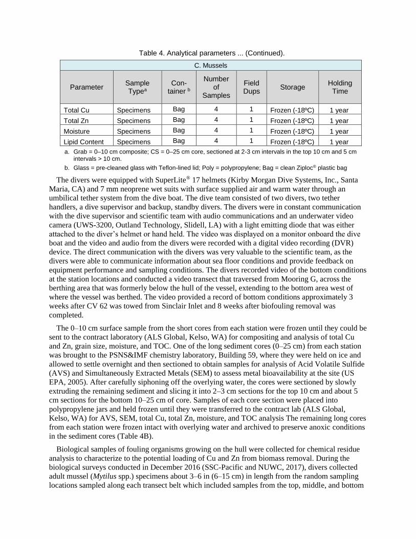
Table 4. Analytical parameters ... (Continued).

C. Mussels


Con-tainer b

Number of

Samples

Field Dups

Storage Holding

Time

Total Cu Specimens Bag 4 1 Frozen (-18ºC) 1 year

Total Zn Specimens Bag 4 1 Frozen (-18ºC) 1 year

Moisture Specimens Bag 4 1 Frozen (-18ºC) 1 year

Lipid Content Specimens Bag 4 1 Frozen (-18ºC) 1 year

a. Grab = 0–10 cm composite; CS = 0–25 cm core, sectioned at 2-3 cm intervals in the top 10 cm and 5 cm intervals > 10 cm.

b. Glass = pre-cleaned glass with Teflon-lined lid; Poly = polypropylene; Bag = clean Ziploc® plastic bag

The divers were equipped with SuperLite® 17 helmets (Kirby Morgan Dive Systems, Inc., Santa

Maria, CA) and 7 mm neoprene wet suits with surface supplied air and warm water through an

umbilical tether system from the dive boat. The dive team consisted of two divers, two tether

handlers, a dive supervisor and backup, standby divers. The divers were in constant communication

with the dive supervisor and scientific team with audio communications and an underwater video

camera (UWS-3200, Outland Technology, Slidell, LA) with a light emitting diode that was either

attached to the diver’s helmet or hand held. The video was displayed on a monitor onboard the dive

boat and the video and audio from the divers were recorded with a digital video recording (DVR)

device. The direct communication with the divers was very valuable to the scientific team, as the

divers were able to communicate information about sea floor conditions and provide feedback on

equipment performance and sampling conditions. The divers recorded video of the bottom conditions

at the station locations and conducted a video transect that traversed from Mooring G, across the

berthing area that was formerly below the hull of the vessel, extending to the bottom area west of

where the vessel was berthed. The video provided a record of bottom conditions approximately 3

weeks after CV 62 was towed from Sinclair Inlet and 8 weeks after biofouling removal was

completed.

The 0–10 cm surface sample from the short cores from each station were frozen until they could be

sent to the contract laboratory (ALS Global, Kelso, WA) for compositing and analysis of total Cu

and Zn, grain size, moisture, and TOC. One of the long sediment cores (0–25 cm) from each station

was brought to the PSNS&IMF chemistry laboratory, Building 59, where they were held on ice and

allowed to settle overnight and then sectioned to obtain samples for analysis of Acid Volatile Sulfide

(AVS) and Simultaneously Extracted Metals (SEM) to assess metal bioavailability at the site (US

EPA, 2005). After carefully siphoning off the overlying water, the cores were sectioned by slowly

extruding the remaining sediment and slicing it into 2–3 cm sections for the top 10 cm and about 5

cm sections for the bottom 10–25 cm of core. Samples of each core section were placed into

polypropylene jars and held frozen until they were transferred to the contract lab (ALS Global,

Kelso, WA) for AVS, SEM, total Cu, total Zn, moisture, and TOC analysis The remaining long cores

from each station were frozen intact with overlying water and archived to preserve anoxic conditions

in the sediment cores (Table 4B).

Biological samples of fouling organisms growing on the hull were collected for chemical residue

analysis to characterize to the potential loading of Cu and Zn from biomass removal. During the

biological surveys conducted in December 2016 (SSC-Pacific and NUWC, 2017), divers collected

adult mussel (Mytilus spp.) specimens about 3–6 in (6–15 cm) in length from the random sampling

locations sampled along each transect belt which included samples from the top, middle, and bottom

of the hull on both the port and starboard sides (Figure 5). Specimens collected from each transect

belt were combined into a single bag (approximately 7–15 individuals). Due to logistics constraints,

it was only possible to sample one location on transect belt 4, therefore, specimens from transect

belts 4 and 5 were combined into a single sample. The samples were stored frozen whole in the shell

until they were transferred to the contract laboratory (ALS Global, Kelso, WA), where they were

thawed, shucked, and composited for analytical analysis of total Cu and Zn, moisture, and lipid

content (Table 4C).

Figure 5. Transect belts around the hull of CV 62 that were sampled during the biological surveys of CV 62 which corresponded to locations were mussel (Mytilus spp.) were collected for residue analysis of Cu, Zn, moisture, and lipid content.

2.2 ANALYTICAL METHODS

Sediments from the Pre- and Post-Removal 0–10 cm surface samples were composited by station and

analyzed for total Cu, total Zn, TOC, and grain size (Table 4). The core section samples were

submitted for analysis of AVS, SEM, total Cu, total Zn, moisture content, and TOC (Table 4). The

mussel tissue samples were submitted for analysis of total Cu and Zn, moisture, and lipid content. All

analyses were conducted by ALS Global (Kelso, WA) under contract to SSC-Pacific (Contract

Number/Purchase Order Agreement N6600117P6856, awarded June 2, 2017). The quality

assurance/quality control (QA/QC) samples used for the project are defined in Table 5, the

recommended acceptance criteria and corrective actions are listed in Table 6, the calculations used to

determine QA/QC statistics are defined in Table 7, and data qualifiers are provided in Table 8. The

details of the analytical analysis and QA/QC procedures followed are detailed below.

Samples selected for total Cu and Zn analyses were stored in a cooler (4º±2°C) or frozen (-18°C)

until submitted for analysis. Archived sample material, if available, was held frozen. Upon submittal

for analysis, samples were thawed, wet homogenized, subsampled for percent moisture, grain size,

and TOC analysis, then freeze-dried and homogenized using a ball-mill prior to digestion. The

subsamples for moisture and grain size were analyzed using Puget Sound Estuary Protocols (PSEP),

TOC was analyzed by ATSM Method D4129M, and the metal samples underwent total digestion and

analysis by Inductively Coupled Plasma – Atomic Emission Spectrometry (ICP-AES) using

procedures recommended by EPA Method 6010B (SW6010B).

The sediment core samples were extracted and analyzed for AVS using US EPA Method EPA-

821-R-100 (Allen et al., 1991; Allen and Fu, 1993). In this method, sulfide in the sample is converted

to hydrogen sulfide by the addition of hydrochloric acid at room temperature. The hydrogen sulfide

(H2S) is purged from the sample by an inert gas and trapped in a sodium hydroxide (NaOH) solution.

With the addition of a mixed-diamine reagent (MDR), the sulfide is converted to methylene blue and

quantified on a spectrometer. The AVS results were reported in units of µmol/g on a dry-weight

basis. The QA/QC samples for the AVS included a MB and LCS. Because AVS is a reactive

substance, MS and SRM are not applicable. The LCS was generated by homogenizing a large

composite field sample and conducting repeated analysis of the sample (n=6) to provide an estimate

of the analytical variance and precision of the method (Johnston, 1993).

The SEM extracts were analyzed for Cd, Cu, Ni, Pb, and Zn by ICP-MS using SW6010B. The

SEM extracts were also analyzed for SEM Hg by Cold Vapor Atomic Absorption (CVAA) using

EPA Method 7470A (US EPA, 1994). The QA/QC samples for SEM analysis included MB, LCS,

MS, MSD, Lab DUPs and SRMs for the analytes of concern. The SEM metal solution concentrations

were determined in units of µg/L and then converted to µg SEM/g of sediment extracted for AVS-

SEM determination. These data were further converted to µmol/g for each SEM metal.

When the molar concentration of AVS are greater than the molar concentration of the sum of the

SEM metals, bioavailability and toxicity of the metals are not expected because the metals are likely

bound as non-soluble sulfides (US EPA, 2005). If sum of SEM (SEM) metals are greater than AVS,

then the metals would be released in order of their sulfide solubility product (Ksp) that expresses the

ratio of dissolved : solid species, where the lower the Ksp the more tightly bound is the metal-sulfide

compound (Morse, Millero, Cornwell, and Rickard, 1987). The SEM metals analyzed were metals of

interest because they have lower sulfide ratios than FeS (Table 9), therefore if the sum of the SEM

metal were greater than AVS, then the metals with the largest sulfide solubility would be present as

potentially toxic free metal (US EPA, 2005). SEM Hg was also analyzed because Hg is a

contaminant of concern for OUB Marine (US Navy, 2012); however, HgS has a much lower sulfide

solubility (2×10-53; URI, 2006) than the other metals so it is very unlikely free Hg would exist in the

presence of AVS.

Table 5 Definitions of QA/QC samples and frequency of analysis.

Sampling Quality Control

QA/QC Sample Definition Frequency

Field Duplicate (DUP)

The field duplicate is a collocated sample defined as a sample collected as near in space and time to the original field sample as the sampling equipment and procedure allows.

1 every ten samples

Equipment Blank (EB) or Field Blank (FB)

The equipment or field blank is collected to assure that sampling apparatus and equipment are free of contamination and that the sampling procedures did not contaminant the sample

1 every sampling event or when specific equipment is used

Laboratory Quality Control

QA/QC Sample Definition Frequency

Method or Procedural Blank (MB)

A combination of solvents, surrogates, and all reagents used during sample processing, processed concurrently with the field samples. Monitors purity of reagents and laboratory contamination.

1/sample batch1.

A processing batch MB must be analyzed with each sequence.

Standard Reference Material (SRM)

An external reference sample which contains a certified level of target analytes; serves as a monitor of accuracy. Extracted and analyzed with samples of a like matrix (may not be available for all analytes)

1/ batch1

Laboratory Control Sample (LCS)

An internal reference sample of known concentration prepared by the performing lab which contains target analytes in similar matrix; serves as a monitor of accuracy when SRM is not available. Extracted and analyzed with samples of a like matrix.

1/ batch1

Matrix Spike (MS)

A field sample spiked with the analytes of interest is processed concurrently with the field samples; monitors effectiveness of method on sample matrix; performed in duplicate.

1/sample batch1

Lab Duplicate Sample

Second aliquot of a field sample processed and analyzed to monitor precision; each sample set should contain a duplicate.

1/sample batch1

Recovery Internal Standards (RIS)

All field and QC samples are spiked with recovery internal standards just prior to analysis; used to quantify surrogates to monitor extraction efficiency on a per sample basis. (Only applicable for GM/MS analysis)

Each sample analyzed for organic compounds

Surrogate Internal Standards (SIS)

All field and QC samples are spiked with a known amount of surrogates just prior to extraction; recoveries are calculated to quantify extraction efficiency. (Only applicable for GC/MS analysis of organic compounds)

Each sample analyzed for organic compounds

1 A batch is defined as 10–20 field samples processed simultaneously and sharing the same QC samples.

Table 6. Measurement QA/QC parameters, acceptance criteria, and suggested corrective actions.

QA/QC Parameter Acceptance Criteria Corrective Action

Method Blank (MB) MB≤MRL If MB>MRL; sample values <10X MB, then perform corrective action

Perform corrective action re-process (extract, digest) sample batch. If batch cannot be re-processed, notify client and flag data.

Standard Reference Material (SRM)

Metals: 20% RPD Determined vs. certified range. Analyte concentration must be > 10xMDL to be used for QC criteria.

Review data to assess impact of matrix. Reanalyze sample and/or document corrective action. If other QC data are acceptable then flag associated data if sample is not reanalyzed.

Matrix Spike (MS)/MS Duplicate (MSD)

Organic compounds: 40–120% recovery Metals: 70–130% recovery Method criteria for all other parameters

Review data to assess impact of matrix. If other QC data are acceptable and no spiking error occurred, then flag associated data. If QC data are not affected by matrix failure or spiking errors occurred, then re-process MS. If not possible, then notify client and flag associated data.

Surrogate Spike (SIS) Organic compounds: 40–120% recovery

Review data. Discuss with Project Manager. Reanalyze, re-extract, and/or document corrective action and deviations.

Laboratory Control Sample (LCS)

AVS: 40–120% recovery Metals: 70–130% recovery Method criteria for all other parameters

Perform corrective action. Re-analyze and/or re-process sample batch. If batch cannot be re-processed: notify client, flag data, discuss impact in report narrative.

Precision: Laboratory Duplicates

Organic compounds (MSD): <30% RPD Metals: <30% RPD Method criteria for all other parameters

Review data to assess impact of matrix. If other QC data are acceptable, then flag associated data. If QC data are not affected by matrix failure, then re-process duplicate. If not possible, then notify client and flag associated data.

Table 7. Calculation of QA/QC Statistics.

Percent Recovery

The percent recovery (PR) is a measurement of accuracy, where one value is compared with a known/certified value. The formula for calculating this value is:

100 x expected amount

detected amount = PR

Table 7. Calculation of QA/QC Statistics. (Continued)

Percent Difference

The percent difference (PD) is a measurement of precision as an indication of how a measured value is difference from a “real” value. It is used when one value is known or certified, and the other is measured. The formula for calculating PD is:

100 x X

X - X = PD

1

12

where: X1 = known value (e.g., SRM certified value)

X2 = determined value (e.g., SRM concentration determined by analyst)

Relative Percent Difference

The relative percent difference (RPD) is a measurement of precision; it is a comparison of two similar samples (matrix spike/matrix spike duplicate pair, field sample duplicates). The formula for calculating RPD is:

100 x )X + X(

)X - X( = RPD

21

21

2/

where: X1 is concentration or percent recovery in sample 1

X2 is concentration or percent recovery in sample 2

Note: Report the absolute value of the result — the RPD is always positive.

Relative Standard Deviation

The relative standard deviation (RSD) is a measurement of precision; it is a comparison of three or more similar samples (e.g., field sample triplicates, initial calibration, MDLs). The formula for calculating RSD is:

𝑅𝑆𝐷 =𝑆𝑡𝑎𝑛𝑑𝑎𝑟𝑑 𝐷𝑒𝑣𝑖𝑎𝑡𝑖𝑜𝑛 𝑜𝑓 𝐴𝑙𝑙 𝑆𝑎𝑚𝑝𝑙𝑒𝑠

𝐴𝑣𝑒𝑟𝑎𝑔𝑒 𝑜𝑓 𝐴𝑙𝑙 𝑆𝑎𝑚𝑝𝑙𝑒𝑠× 100

Table 8. Data Qualifiers used by the contract lab (ALSGlobal).

Inorganic Data Qualifiers

* The result is an outlier. See case narrative.

# The control limit criteria is not applicable. See case narrative.

B The analyte was found in the associated method blank at a level that is significant relative to the sample result as defined by the DOD or NELAC standards.

E The result is an estimate amount because the value exceeded the instrument calibration range.

Table 8. Data Qualifiers used by the contract lab (ALSGlobal). (Continued)


J The result is an estimated value.

U The analyte was analyzed for, but was not detected (“Non-detect”) at or above the MRL/MDL.

DOD-QSM 4.2 definition: Analyte was not detected and is reported as less than the LOD or as defined by the project. The detection limit is adjusted for dilution.

i The MRL/MDL or LOQ/LOD is elevated due to a matrix interference.


X See case narrative.

Q See case narrative. One or more quality control criteria was outside the limits.

H The holding time for this test is immediately following sample collection. The samples were analyzed as soon as possible after receipt by the laboratory.

Metals Data Qualifiers

# The control limit criteria is not applicable. See case narrative.

J The result is an estimated value.

E The percent difference for the serial dilution was greater than 10%, indicating a possible matrix interference in the sample.

M The duplicate injection precision was not met.

N The Matrix Spike sample recovery is not within control limits. See case narrative.

S The reported value was determined by the Method of Standard Additions (MSA).

U The analyte was analyzed for, but was not detected (“Non-detect”) at or above the MRL/MDL.

DOD-QSM 4.2 definition: Analyte was not detected and is reported as less than the LOD or as defined by the project. The detection limit is adjusted for dilution.

W The post-digestion spike for furnace AA analysis is out of control limits, while sample absorbance is less than 50% of spike absorbance.

i The MRL/MDL or LOQ/LOD is elevated due to a matrix interference.

X See case narrative.

+ The correlation coefficient for the MSA is less than 0.995.

Q See case narrative. One or more quality control criteria was outside the limits.

Table 9. Metal-sulfide* solubility products and ratios (from US EPA, 2005).

*Metal-Sulfide (MeS) equilibrium of the type:

MeS(s) + H+ Me2+(aq) + HS–(aq)

Sediment quality benchmarks for the protection of benthic organisms from metal exposure have

been developed based on the knowledge of AVS, the sum of the simultaneously extracted metals

(SEM), and fraction of organic carbon (fOC) in the sediment (US EPA, 2005):

Low risk of adverse biological effects

Equation 1: (SEM - AVS)/fOC ≤ 130 mol/g OC

May have adverse biological effect

Equation 2: 130 mol/g OC < (SEM - AVS)/foc ≤ 3000 mol/g OC

Adverse biological effects expected

Equation 3: (SEM - AVS)/foc > 3000 mol/g OC

2.3 DATA ANALYSIS

Statistical analyses were performed to determine if there were statistically-significant differences

between Pre- and Post-Biofouling Removal for total Cu, total Zn, grain size fractions, solids content,

and TOC. Data from the sampling were evaluated in the context of historical Cu and Zn data

available for the site which includes investigations for Operable Unit B Marine (OUB Marine, US

Navy; 2012), the ENVVEST (Environmental Reinvestment) program (US Navy, US EPA, and

Ecology, 2000), studies conducted by the Navy and participating stakeholders (ENVVEST 2006), an

activated carbon sediment amendment demonstration project conducted at Pier 7 of PSNS&IMF

(Kirtay et al., 2017), and Sinclair Inlet monitoring conducted by Ecology's sediment monitoring

program (Weakland et al., 2013).

2.3.1.1 Statistical Analysis

The raw data were validated based on the pre-defined performance based QA/QC procedures

identified in the PWP (SSC-Pacific and NUWC, 2016) and all useable data were combined into a flat

file (MS Excel, Microsoft Inc., Redman, WA) for statistical analysis. The flat file was imported into

R-Studio (v98.1091, r-studio.com, Boston, MA) running R (v3.01.1, R Foundation for Statistical

Computing, www.r-project.org) for statistical analysis. Descriptive statistics were compiled for the

data for the Pre- and Post- sampling events and corresponding tables and plots showing the data were

prepared. A hypothesis was developed based on the traditional Before – After design:

Ho: There are no differences between variables measured prior to biofouling removal (Pre-) and

the same variables measured after the ship was cleaned and towed (Post-) from Sinclair Inlet.

Prior to conducting statistical tests, histograms of the data were plotted to determine whether the

data distribution conformed to a normal or lognormal distribution and were suitable for parametric

analysis of variance (ANOVA) or would be better evaluated using non-parametric statistical tests that

do not require assumptions of normality. For practicality, both parametric and non-parametric tests

were calculated to test the hypothesis.

For Ho the following tests were used

Equation 4: Parametric ANOVANormal: F = aov(Y ~ Event, data = Sediment)

Equation 5: Parametric ANOVALogormal: F = aov(log(Y) ~ Event, data = Sediment)

Equation 6: Non-Parametric: KW = kruskal.test(Y ~ Event, data = Sediment)

Where

Y = variable of interest

log(Y) = log base 10 transformed data for variable Y

Event = Pre- or Post-Biofouling Removal

Sediment = sediment raw data set

And

F and KW = statistical result for ANOVA or Kruskal-Wallis non-parametric tests,

respectively

p(F) and p(KW) = probability of random result, and

p ≤ 0.05 denotes statistical significance

Box and whisker plots (Figure 6) by event were constructed to visualize statistical comparisons

and evaluate the magnitude of the differences detected. Core profiles were constructed with the data

from the core sections collected Post-Removal to illustrate the distribution of moisture content, TOC,

total Cu, total Zn, AVS, and SEM present in the sediments of the site. The probability of exceeding

sediment quality benchmarks for the protection of benthic organisms was calculated by pooling the

sediment core data by depth, calculating the mean ( ) and standard deviation ( ) for Y = (SEM -

AVS)/foc, and estimating the probability of exceeding the benchmarks using the Excel NORM.DIST

function:

Equation 7: P(Bx) = 1 - NORM.DIST(Bx,,,TRUE)

Where

Bx = Sediment benchmark of interest {130 mol/g OC, 3000 mol/g OC}

= mean of the data distribution, and

= standard deviation of the data distribution, and

NORM.DIST(Bx,,,TRUE) returns the cumulative distribution with a mean of ,

standard deviation of for Bx

The probability of exceeding the benchmarks was calculated assuming a normal distribution {,

} and lognormal distribution {^, ^}

Equation 8: P(Bx^) = 1 - NORM.DIST(Bx

^,^,^,TRUE)

where the data were log transformed using the following transformation:

Equation 9: Y^ = log[(SEM - AVS)/fOC +2000]

The probability obtained from the lognormal distribution is more conservative than the probability

calculated from the normal distribution because the lognormal distribution includes the values that

form a long tail to the right of the distribution.

Figure 6. Statistical parameters depicted in a typical box and whisker plot showing the median (line), the first and third quartile (box), the inner quartile range, and range of the data (whiskers). Figure from http://www.physics.csbsju.edu/stats/box2.html.

2.3.2 Decision Framework

A decision matrix (Table 10) was used to evaluate whether biofouling removal caused any impacts

to sediment quality in Sinclair Inlet. The decision takes into account whether there were statistical

differences between the Pre- and Post- Removal sampling events, the magnitude of the difference,

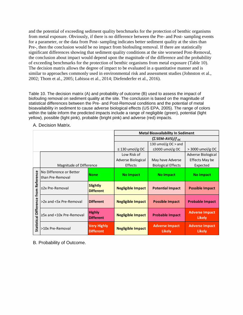
http://www.physics.csbsju.edu/stats/box2.html

and the potential of exceeding sediment quality benchmarks for the protection of benthic organisms

from metal exposure. Obviously, if there is no difference between the Pre- and Post- sampling events

for a parameter, or the data from Post- sampling indicates better sediment quality at the sites than

Pre-, then the conclusion would be no impact from biofouling removal. If there are statistically

significant differences showing that sediment quality conditions at the site worsened Post-Removal,

the conclusion about impact would depend upon the magnitude of the difference and the probability

of exceeding benchmarks for the protection of benthic organisms from metal exposure (Table 10).

The decision matrix allows the degree of impact to be evaluated in a quantitative manner and is

similar to approaches commonly used in environmental risk and assessment studies (Johnston et al.,

2002; Thom et al., 2005; Labisoa et al., 2014; Diefenderfer et al., 2016).

Table 10. The decision matrix (A) and probability of outcome (B) used to assess the impact of biofouling removal on sediment quality at the site. The conclusion is based on the magnitude of statistical differences between the Pre- and Post-Removal conditions and the potential of metal bioavailability in sediment to cause adverse biological effects (US EPA, 2005). The range of colors within the table inform the predicted impacts include a range of negligible (green), potential (light yellow), possible (light pink), probable (bright pink) and adverse (red) impacts.

A. Decision Matrix.

B. Probability of Outcome.

≤ 130 umol/g OC

130 umol/g OC > and

≤3000 umol/g OC > 3000 umol/g OC

Low Risk of

Adverse Biological

Effects

May have Adverse

Biological Effects

Adverse Biological

Effects May be

Expected

No Difference or Better

than Pre-RemovalNone No Impact No Impact No Impact

≤2x Pre-RemovalSlightly

DifferentNegligible Impact Potential Impact Possible Impact

>2x and <5x Pre-Removal Different Negligible Impact Possible Impact Probable Impact

≥5x and <10x Pre-RemovalHighly

DifferentNegligible Impact Probable Impact

Adverse Impact

Likely

>10x Pre-RemovalVery Highly

DifferentNegligible Impact

Adverse Impact

Likely

Adverse Impact

Likely

Magnitude of Difference

Stat

isti

cal D

iffe

ren

ce f

rom

Ref

eren

ce

Metal Bioavailability In Sediment

(SEM-AVS)/f OC


Probability of Outcome P

Very Low < 2%

Low ≥ 2% < 10%

Medium ≥ 10% < 50%

High ≥ 50% < 80%

Very High ≥ 80%

23

3. RESULTS

The raw data and QA/QC narrative from chemistry analysis reported by ALS Global, Inc. are

provided in Appendix A for Pre-Removal sediment grabs (Appendix A-1), Post-Removal sediment

grabs (Appendix A-2), AVS cores (Appendix A-3), and mussel tissues (Appendix A-4). The raw

taxonomic data obtained from the Pre-Removal sampling are provided in Appendix B. Video clips

from the underwater surveys of the hull of CV 62 prior to biofouling removal and the sea floor after

CV 62 was towed from Sinclair Inlet are provided in Appendix C. Appendix D provides all the data

from the study in the electronic data deliverable (EED) format required for submission to Ecology’s

Environmental Information Management (EIM) system (Ecology, 2017). Printed versions of the

report include a CD that contains additional content for Appendices A–D.

3.1 QA/QC REVIEW

The analytical chemistry data were evaluated to assure accuracy, precision, completeness,

comparability, and representativeness of the analytical results. The data were validated according to

the QA/QC procedures defined in the QAP and the raw data were flagged with appropriate qualifier

codes, if applicable (see Appendix A). The analytical parameters, holding times prior to analysis, the

methods used, the method reporting limits (MRL), and method detection limits (MDL) are

summarized in Table 11. No anomalies were reported for the analytical results for the Pre- and Post-

Removal sediment surface samples, mussel tissue samples, and TOC, and moisture analysis of the

core sections.

For the AVS analysis of the cores sections, the contract lab reported that acceptable recovery

levels for sulfide SRM was not achieved, however, the AVS digestion is less aggressive than

normally used for total sulfide analysis and low recovery of the sulfide SRM was expected. To

address sulfide accuracy and precision, the contract lab was requested to perform AVS analysis on 6

replicate aliquots from one field sample to demonstrate proficiency and accuracy (Laboratory

Control Sample – LCS). The results from the repeated analysis showed that AVS was highly variable

with an adjusted coefficient of variation (CoefV* = / × (1 + 1/4n) × 100; Sokal and Rohlf, 1995)

of 41% (Table 12). The variability was likely due to sample inhomogeneity and laboratory variation.

Sample inhomogeneity was also the likely cause of the high RPD outside of control limits, obtained

for laboratory duplicates in the metals analysis of the AVS cores (Appendix A-3).

The AVS is very susceptible to oxidation (US EPA, 2005), so the samples were stored frozen in

tightly sealed polycarbonate jars. However, there was head space in the jars and the amount of

material collected in the core sections was highly variable due to shells, rocks, and other debris

present in the samples. This resulted in varying amounts of exposed surface of the sample that could

have been oxidized during storage. The contract lab was requested to remove the oxidized surface

level prior to homogenization, but because of limited sample size and standardized sample

processing procedures performed by the lab it is not clear how well this request was carried out. The

ideal situation would be to process the fresh cores immediately after collection or after thawing and

sectioning intact cores (Johnston, 1993; US EPA, 2005), however, this was not possible due to

contracting procedures and logistical limitations.

The sediment surface samples (0–10 cm) were collected prior to biofouling removal on December

12, 2016 (Pre-Removal) and on March 30, 2017 after the ship was towed from Sinclair Inlet (Post-

Removal). In addition, the Post-Removal sampling included collecting 0–25 cm core samples from

the stations. The analytical chemistry results for the sediment grabs are provided in Table 13 and

Table 14 presents the results obtained for the sediment core sections.

24

Table 11. The analytical parameters, dates collected and analyzed, holding times prior to analysis, methods used, the method reporting limit (MRL), method detection limit (MDL), and reporting units achieved for Pre-Removal sediment (A), Post-Removal sediment (B), and mussel tissue samples (C) collected during the study.

Table 12. The results of AVS analysis of six replicate aliquots conducted to determine laboratory proficiency and accuracy.

Replicate AVS mol/g wet

CV62AVS-19 Field SRM1 12.7






Mean (µ) 12.7

Standard Deviation (σ) 5.0

CoefV* 41%

Extraction

or AnalysisAnalysis

Parameter

Date

Colleted Storage

Date

Extracted

Date

Analyzed Months

Days After

Extraction Method MRL MDL units

Cu 12/13/2016 4C 6/9/2017 6/27/2017 5.93 18 SW6010C 2.4 0.9 ug/g dry

Zn 12/13/2016 4C 6/9/2017 6/27/2017 5.93 18 SW6010C 2.5 0.5 ug/g dry

Solids 12/13/2016 4C 6/9/2017 5.93 PSEP TS % wet

TOC 12/13/2016 4C 6/29/2017 6.60 ASTMD4129M 0.05 0.02 % dry

Grain Size 12/13/2016 4C 6/15/2017 6.13 PSEP Grain Size % dry

Cu Grab 3/30/2017 Frozen(-18C) 6/9/2017 6/27/2017 2.37 18 SW6010C 1.25 0.48 ug/g dry

Zn Grab 3/30/2017 Frozen(-18C) 6/9/2017 6/27/2017 2.37 18 SW6010C 1.56 0.31 ug/g dry

Solids 3/30/2017 Frozen(-18C) 6/9/2017 2.37 PSEP TS % wet

TOC 3/30/2017 Frozen(-18C) 6/29/2017 3.03 ASTMD4129M 0.05 0.02 % dry

Grain Size 3/30/2017 Frozen(-18C) 6/15/2017 2.57 PSEP Grain Size % dry

Cu Core Sections 3/30/2017 Frozen(-18C) 6/28/2017 6/29/2017 3.00 1 SW6010C 1.6 0.6 ug/g dry

Zn Core Sections 3/30/2017 Frozen(-18C) 6/28/2017 6/29/2017 3.00 1 SW6010C 2.0 0.4 ug/g dry

AVS 3/30/2017 Frozen(-18C) 6/28/2017 6/29/2017 3.00 1 821/R-91-100 3.55 0.97 umol/g dry

SEM Cd 3/30/2017 Frozen(-18C) 6/28/2017 6/29/2017 3.00 1 SW6010C 0.0017 0.0006 umol/g dry

SEM Cu 3/30/2017 Frozen(-18C) 6/28/2017 6/29/2017 3.00 1 SW6010C 0.058 0.014 umol/g dry

SEM Pb 3/30/2017 Frozen(-18C) 6/28/2017 6/29/2017 3.00 1 SW6010C 0.009 0.004 umol/g dry

SEM Hg 3/30/2017 Frozen(-18C) 6/28/2017 6/29/2017 3.00 1 7470A 0.00034 0.00007 umol/g dry

SEM Ni 3/30/2017 Frozen(-18C) 6/28/2017 6/29/2017 3.00 1 SW6010C 0.009 0.003 umol/g dry

SEM Zn 3/30/2017 Frozen(-18C) 6/28/2017 6/29/2017 3.00 1 SW6010C 0.050 0.020 umol/g dry

Cu 12/10/2016 Frozen(-18C) 7/3/2017 7/10/2017 6.83 7 SW6010C 0.07 0.04 ug/g wet

Zn 12/10/2016 Frozen(-18C) 7/3/2017 7/10/2017 6.83 7 SW6010C 0.07 0.04 ug/g wet

Solids 12/10/2016 Frozen(-18C) 6/30/2017 6/30/2017 6.73 FreezeDry % wet

Lipids 12/10/2016 Frozen(-18C) 6/29/2017 7/6/2017 6.70 7 NLIPIDS 0.16 % wet

Holding Time

A. Pre-Removal Sediment Samples

B. Post-Removal Sediment Samples

C. Mussel Tissue Samples

25

Table 13. Analytical chemistry results for Pre-Removal (A) and Post-Removal (B) 0-10 cm surface samples. Data are shown for the concentration of metals (Cu and Zn), and percent of gravel, sand, clay, very coarse sand (VCSa), coarse sand (CSa), medium sand (MSa), very fine sand (VFSa), fines (Fines = Silt + Clay), total organic carbon (TOC), and solids in each sample. The results of the field duplicate are also provided to assess field variability. The results are on a dry weight basis, except for solids, which are on a wet-weight basis.

A. Surface sampling (0–10 cm) results Pre-Removal.

B. Surface sampling (0–10 cm) results Post-Removal.

Cu Zn Gravel Sand Silt Clay VCSa CSa MSa FSa VFSa Fines TOC Solids

Location_ID Sample_ID

CV62-1 CV62SED-01 12/13/2016 200 229 0.00 1.50 68.37 33.04 0.1 0.2 0.2 0.2 0.8 98.5 3.78 22.40

CV62-2 CV62SED-02 12/13/2016 170 420 32.34 14.98 34.03 13.68 3.9 2.0 1.2 1.8 6.0 50.2 2.73 41.20

CV62-3 CV62SED-03 12/13/2016 180 203 0.98 4.28 69.41 28.53 1.0 0.4 0.6 0.4 1.8 94.9 3.30 27.00

CV62-4 CV62SED-04 12/13/2016 146 163 0.36 2.07 72.58 26.27 0.4 0.2 0.2 0.2 1.2 97.6 3.23 27.70

CV62-51

CV62SED-05,06 12/13/2016 207 181 0.28 2.07 69.23 30.94 0.3 0.2 0.2 0.4 1.0 97.7 3.89 23.45

CV62-6 CV62SED-07 12/13/2016 206 215 1.83 2.72 69.85 31.43 0.5 0.4 0.2 0.5 1.2 95.7 3.54 28.90

6 6 6 6 6 6 6 6 6 6 6 6 6 6

146.0 163.0 0.0 1.5 34.0 13.7 0.1 0.2 0.2 0.2 0.8 50.2 2.7 22.4

184.8 235.2 6.0 4.6 63.9 27.3 1.0 0.6 0.4 0.6 2.0 89.1 3.4 28.4

24.1 93.6 12.9 5.2 14.7 7.1 1.5 0.7 0.4 0.6 2.0 19.1 0.4 6.7

206.5 420.0 32.3 15.0 72.6 33.0 3.9 2.0 1.2 1.8 6.0 98.5 3.9 41.2

13.6% 41.5% 226.0% 117.1% 24.0% 27.0% 147.2% 131.1% 101.9% 110.1% 104.3% 22.3% 12.9% 24.7%

Field Duplicate

CV62-5 CV62SED-05 12/13/2016 242 175 0.15 1.67 70.53 32.24 0.23 0.19 0.19 0.21 0.85 102.8 3.89 22.8

CV62-5DUP CV62SED-06 12/13/2016 171 187 0.40 2.47 67.92 29.64 0.27 0.24 0.17 0.56 1.23 97.6 3.88 24.1

34.38% 6.63% 90.91% 38.65% 3.77% 8.40% 16.00% 23.26% 11.11% 90.91% 36.54% 5.20% 0.26% 5.54%1.

Average of Field Duplicates

min

n

RPD

CV*

ug/g percent

Collection

Date

stdev

max

mean

Parameter

Cu Zn Gravel Sand Silt Clay VCSa CSa MSa FSa VFSa Fines TOC Solids

Location_ID Sample_ID

CV62-1 CV62SED-51 3/30/2017 240 208 0 2.36 76.34 31.39 0.0 0.1 0.3 0.6 1.4 97.9 3.72 11.80

CV62-2 CV62SED-52 3/30/2017 82 245 60.09 28.46 6.93 3.27 9.3 8.8 7.1 1.5 1.7 10.3 0.59 62.00

CV62-3 CV62SED-53 3/30/2017 778 314 19.12 9.47 55.74 22.65 2.9 1.4 1.3 1.7 2.2 73.3 3.60 27.60

CV62-4 CV62SED-54 3/30/2017 169 1200 1.44 2.03 75.41 24.31 0.4 0.2 0.2 0.3 0.9 96.6 3.34 26.10

CV62-5 CV62SED-55 3/30/2017 432 242 1.21 5.42 67.09 27.60 0.4 0.4 0.4 1.3 3.0 93.5 3.50 27.90

CV62-61 CV62SED-56,57 3/30/2017 472 252 8.93 6.41 60.63 27.79 2.6 1.2 0.7 0.7 1.3 85.2 4.28 24.25

6 6 6 6 6 6 6 6 6 6 6 6 6 6

82.0 208.0 0.0 2.0 6.9 3.3 0.0 0.1 0.2 0.3 0.9 10.3 0.6 11.8

362.1 410.2 15.1 9.0 57.0 22.8 2.6 2.0 1.7 1.0 1.7 76.1 3.2 29.9

253.2 388.5 23.2 9.9 25.8 10.1 3.5 3.4 2.7 0.6 0.7 33.5 1.3 16.8

778.0 1200.0 60.1 28.5 76.3 31.4 9.3 8.8 7.1 1.7 3.0 97.9 4.3 62.0

72.8% 98.7% 159.6% 114.4% 47.2% 45.9% 139.6% 172.3% 170.4% 59.7% 44.1% 45.8% 42.8% 58.5%

Field Duplicate

CV62-6 CV62SED-56 3/30/2017 678 284 9.67 4.16 58.74 27.09 1.35 0.72 0.47 0.45 1.17 85.8 4.11 25.3

CV62-6DUP CV62SED-57 3/30/2017 265 220 8.19 8.65 62.51 28.49 3.85 1.66 0.89 0.89 1.36 91.0 4.44 23.2

87.59% 25.40% 16.57% 70.10% 6.22% 5.04% 96.15% 78.99% 61.76% 65.67% 15.02% 5.85% 7.72% 8.66%1.

Average of Field Duplicates

Parameter

Collection

Date ug/g percent

RPD

n

min

mean

stdev

max

CV*

26

Table 14. Results for individual core sections (A), core sections averaged for 0–10 cm depth interval (B), core sections averaged for depth > 10 cm (C) of AVS, SEM metals, TOC, solids, and total Cu and Zn. Shaded cells indicate parameter not detected at the MDL shown.

A. Core section results Post-Removal.

Core Depth Avg Depth AVS SEM_Cd SEM_Cu SEM_Pb SEM_Hg SEM_Ni SEM_Zn SEM SEM-AVS (SEM-AVS)/foc TOC Solids Cu Zn

Location cm cm mol/g OC % dry % wet

0 1.5 0.11 0.021 1.80 0.262 0.00012 0.176 2.42 4.68 4.57 120.24 3.80 19.0 184 186

3 4.5 7.30 0.016 1.25 0.253 0.00006 0.101 2.40 4.02 -3.28 -85.63 3.83 23.8 268 279

6 8 0.41 0.021 1.86 0.326 0.00005 0.121 3.22 5.55 5.14 135.56 3.79 27.9 250 296

10 12.5 15.20 0.013 0.72 0.216 0.00006 0.089 1.83 2.87 -12.33 -322.02 3.83 25.4 232 261

15 17.5 12.40 0.015 1.31 0.197 0.00007 0.111 1.84 3.47 -8.93 -293.64 3.04 33.1 171 156

20 23 16.50 0.010 0.59 0.203 0.00006 0.080 1.71 2.59 -13.91 -374.92 3.71 26.8 240 257

26

0 2 46.00 0.011 0.33 0.189 0.00006 0.078 1.82 2.42 -43.58 -1174.56 3.71 25.0 236 287

4 7 2.33 0.007 0.68 2.020 0.00004 0.098 8.25 11.05 8.72 1207.79 0.72 75.7 106 248

10

0 2.5 4.80 0.005 0.37 0.899 0.00004 0.135 17.00 18.41 13.61 3057.47 0.45 83.9 127 585

5 7.5 13.00 0.059 7.27 0.213 0.00009 0.124 21.40 29.07 16.07 586.37 2.74 24.4 23400 7400

10 12 45.00 0.017 0.36 0.142 0.00006 0.110 4.94 5.57 -39.43 -1355.01 2.91 37.1 201 257

14

0 1.5 18.20 0.021 2.31 0.166 0.00006 0.104 6.70 9.30 -8.90 -436.22 2.04 40.2 183 227

3 4.5 0.05 0.012 1.05 0.165 0.00009 0.084 1.35 2.66 2.61 82.89 3.15 18.5 124 137

6 8 0.06 0.012 1.40 0.156 0.00012 0.098 1.55 3.22 3.16 100.20 3.15 22.5 163 165

10 12.5 0.26 0.012 1.24 0.165 0.00006 0.213 1.53 3.16 2.90 92.06 3.15 24.3 376 151

15 19 25.10 0.015 0.81 0.187 0.00006 0.114 1.54 2.67 -22.43 -686.01 3.27 26.0 147 147

23

0 2.5 45.20 0.011 0.25 0.139 0.00006 0.092 1.63 2.12 -43.08 -1398.57 3.08 28.2 138 232

5 7.5 8.70 0.019 2.53 0.213 0.00010 0.130 3.36 6.25 -2.45 -55.12 4.44 24.7 1510 287

10 14.5 41.60 0.018 1.09 0.222 0.00008 0.126 2.08 3.54 -38.06 -1093.78 3.48 30.0 240 203

19

0 2.5 64.00 0.011 0.50 0.424 0.00005 0.147 16.30 17.38 -46.62 -1857.35 2.51 42.7 1810 282

5 7.5 10.30 0.009 0.87 0.151 0.00007 0.078 1.34 2.45 -7.85 -487.66 1.61 38.7 163 121

10 12.5 24.30 0.012 1.22 0.156 0.00006 0.106 1.77 3.26 -21.04 -703.54 2.99 36.8 354 173

15 17.5 32.50 0.019 1.64 0.261 0.00009 0.151 2.35 4.42 -28.08 -630.98 4.45 25.7 452 264

20

Summary AVS SEM_Cd SEM_Cu SEM_Pb SEM_Hg SEM_Ni SEM_Zn SEM SEM-AVS (SEM-AVS)/foc TOC Solids Cu Zn

n 23 23 23 23 23 23 23 23 23 23 23 23 23 23

min 0.05 0.005 0.25 0.14 0.00004 0.08 1.34 2.12 -46.62 -1857.35 0.45 18.50 106 121

average 18.84 0.016 1.37 0.32 0.12 4.71 6.53 -12.31 -242.28 3.04 33.06 1351 548

median 13.00 0.013 1.09 0.20 0.11 2.08 3.54 -8.90 -322.02 3.15 26.80 232 248

max 64.00 0.059 7.27 2.02 0.00012 0.21 21.40 29.07 16.07 3057.47 4.45 83.90 23400 7400

CV62-4

CV62-5

CV62-6

CV62-3

mol/g dry weight g/g dry weight

CV62-1

CV62-2

27

Table 14. Results for individual core sections ... (Continued).

B. Core section results Post-Removal average for 0–10 cm depth.

C. Core section results Post-Removal average for > 10 cm depth.

AVS SEM_Cd SEM_Cu SEM_Pb SEM_Hg SEM_Ni SEM_Zn SEM SEM-AVS (SEM-AVS)/foc TOC Solids Cu Zn

umol/g OC % dry % wet

2.61 0.019 1.64 0.28 0.13 2.68 4.75 2.14 56.73 3.81 23.57 234 254

24.17 0.009 0.50 1.10 0.09 5.04 6.74 -17.43 16.61 2.22 50.35 171 268

8.90 0.032 3.82 0.56 0.13 19.20 23.74 14.84 1821.92 1.59 54.15 11764 3993

6.10 0.015 1.59 0.16 0.10 3.20 5.06 -1.04 -84.38 2.78 27.07 157 176

26.95 0.015 1.39 0.18 0.11 2.50 4.19 -22.76 -726.85 3.76 26.45 824 260

37.15 0.010 0.68 0.29 0.11 8.82 9.91 -27.24 -1172.51 2.06 40.70 987 202

17.65 0.017 1.60 0.43 0.11 6.91 9.06 -8.58 -14.75 2.70 37.05 2356 859

13.75 0.008 1.18 0.36 0.02 6.47 7.48 16.42 1022.92 0.92 13.24 4623 1536

B. Average for 0-10 cm depth

umol/g dry weight ug/g dry weightLocation

CV62-1

CV62-2

CV62-3

CV62-4

CV62-5

CV62-6

Overall average 0-10 cm

Overall stdev 0-10 cm

AVS SEM_Cd SEM_Cu SEM_Pb SEM_Hg SEM_Ni SEM_Zn SEM SEM-AVS (SEM-AVS)/foc TOC Solids Cu Zn

Location Max Depth cm umol/g OC % dry % wet

CV62-1 26 14.70 0.013 0.87 0.21 0.09 1.79 2.98 -11.72 -330.19 3.53 28.43 214 225

CV62-2

CV62-3 14 45.00 0.017 0.36 0.14 0.11 4.94 5.57 -39.43 -1355.01 2.91 37.10 201 257

CV62-4 23 12.68 0.013 1.03 0.18 0.16 1.54 2.91 -9.77 -296.97 3.21 25.15 262 149

CV62-5 19 41.60 0.018 1.09 0.22 0.13 2.08 3.54 -38.06 -1093.78 3.48 30.00 240 203

CV62-6 20 28.40 0.016 1.43 0.21 0.13 2.06 3.84 -24.56 -667.26 3.72 31.25 403 219

Avg Core depth 20.4

28.48 0.015 0.96 0.19 0.12 2.48 3.77 -24.71 -748.64 3.37 30.39 264 210

14.87 0.002 0.39 0.03 0.03 1.39 1.08 14.03 467.05 0.31 4.39 81 40Overall stdev >10 cm

Overall average >10 cm

umol/g dry weight ug/g dry weight

28

3.2 PRE-AND POST-REMOVAL SEDIMENT SURFACE SAMPLES

The sediment surface samples were collected to document conditions in the surface sediment

before and after biofouling removal. The Pre-Removal surface samples collected by ponar grabs

were observed to be very soft, unconsolidated material, with a black jelly-like consistency, smelling

strongly of sulfide, and no evidence of any oxidation or bioturbation. Shell material and other debris

were also observed in the samples. Samples with similar consistency were reported by the divers

when they collected the Post-Removal surface samples and cores. The divers encountered shell hash

and other debris on the sea floor which was recorded on the video feed. While different sampling

methods were used for the Pre- (ponar grab) and Post-Removal (diver-collected 0–10 cm core)

sampling events, both methods provided equivalent results as they uniformly sampled the 0–10 cm

surface layer present. The advantage of using divers to collect the samples Post-Removal was that the

divers were able to avoid any obstruction from biological material that was present on the sea floor

and thus, avoided problems of shell and debris that could prevent the ponar-sampler from obtaining

an intact sample by not closing properly. Both sampling methods met the Data Quality Objective of

collecting an undisturbed uniform sample of the 0–10 cm surface sediment layer, which was verified

by the field sampling team.

The analytical chemistry results for the 0–10 cm Pre- and Post-Removal surface samples are

presented in Table 13. Data are shown for the concentration of total metals (Cu and Zn), and percent

of gravel, sand, clay, very coarse sand (VCSa), coarse sand (CSa), medium sand (MSa), very fine

sand (VFSa), Fines (Fines = (Silt + Clay)/(Gravel + Sand + Silt + Clay)), total organic carbon (TOC),

and Solids in each sample. The results of the field duplicates were used to assess field variability; the

RPD reported indicates the range of difference needed to differentiate one sample from another.

There were three stations (CV62-3, CV62-5, and CV62-6) where the Post-Removal total Cu

concentration was greater than Pre-Removal concentration at levels above the RPD for field

duplicates and these stations exceeded the Maximum Criteria Concentration (MCC) benchmark for

Cu (Figure 7A). For total Zn, four stations (CV62-3, CV62-4, CV62-5, and CV62-6) had Post-

Removal concentrations that were greater than Pre-Removal concentrations at levels above the RPD

for field duplicates, but only CV62-4 exceeded the MCC benchmark for Zn (Figure 7B).

29

Figure 7. The concentration of total Cu (A) and Zn (B) measured in Pre- and Post-Removal 0–10 cm surface samples collected at each station location. The sediment quality benchmarks are shown for the Sediment Quality Standard (SQS, green dotted line) and Maximum Chemical Criteria (MCC, dashed red lines). Error bars are standard deviation of field duplicates.

30

On average, Pre-Removal grab samples contained lower total Cu (average 191 g/g Cu dry

weight) and lower total Zn (average 234 g/g Zn dry weight) than the Post-Removal concentrations

(average 397 g/g Cu dry weight and 416 g/g Zn dry weight). However, these differences were not

statistically significant at p ≤ 0.05 confidence level (Table 15). The lack of statistical significance

between the two sampling periods was primarily due to the high variability of the results for both

sampling periods (Figure 8). Significance tests calculated for the ANOVANormal (Equation 4),

ANOVALognormal (Equation 5), and nonparametric KW (Equation 6) distributions were all in

agreement (Table 15). The difference in Zn concentrations Pre- and Post- were statistically

significant at the p ≤ 0.10 level, the difference was driven by the Post-Removal sample from CV62-4

that was much higher than all the other samples (Figure 7B, Figure 8B).

Figure 8. Box and whisker plot for concentrations of Cu (A) and Zn (B) measured in in Pre- and Post-Removal 0-10 cm surface sediment samples collected at each station location. The data (black points), Sediment Quality Standard (SQS, green dotted line), and Maximum Chemical Criteria (MCC, red dashed lines) are also shown. See Figure 6 for description of box and whisker statistical parameters.

31

Table 15. Results from statistical tests to determine if there were significant differences between variables measured in 0–10 cm grabs assuming normal, lognormal, and non-parametric distributions for the data. The relative difference between average Pre- and Post-Removal variables is also tabulated.

There were no statistically significant differences (p ≤ 0.05) for TOC and Solids between sampling

events (Figure 9, Figure 10, and Table 15), however, station CV62-2 had much less TOC and greater

percent solids in the sample collected Post-Removal (Figure 9). There were also no statistically

significant differences (p ≤ 0.05) for the content of gravel, sand, silt, and clay between the Pre- and

Post- samples (Figure 11, Figure 12, Table 15), although changes to more coarse material and less

fines were evident in the samples from CV62-2, CV62-3, and CV62-6 (Figure 11).

Figure 9. The percent TOC (A) and solids (B) measured in Pre- and Post-Removal 0–10 cm surface sediment samples collected at each station location.

ANOVANormal ANOVALognormal Non-Parametric

Variable P(F) P(F) P(KW) Difference

Cu ug/g 0.118 0.221 0.262 2.1

Zn ug/g 0.309 0.240 0.078 1.8

Gravel % 0.417 0.221 0.298 2.6

Sand % 0.356 0.265 0.262 1.9

Silt % 0.583 0.461 0.631 0.9

Clay % 0.393 0.391 0.200 0.8

TOC % 0.677 0.489 0.749 0.9

Solids % 0.843 0.850 0.873 1.1

Distribution

32

Figure 10. Box and whisker plot for percent solids (A) and TOC (B) measured in in Pre- and Post-Removal 0–10 cm surface sediment samples collected at each station location. The data (black points) are also shown. See Figure 6 for description of box and whisker statistical parameters.

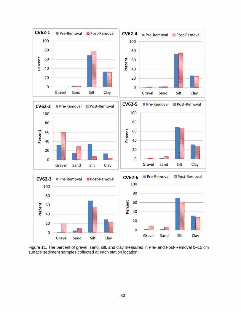
33

Figure 11. The percent of gravel, sand, silt, and clay measured in Pre- and Post-Removal 0–10 cm surface sediment samples collected at each station location.

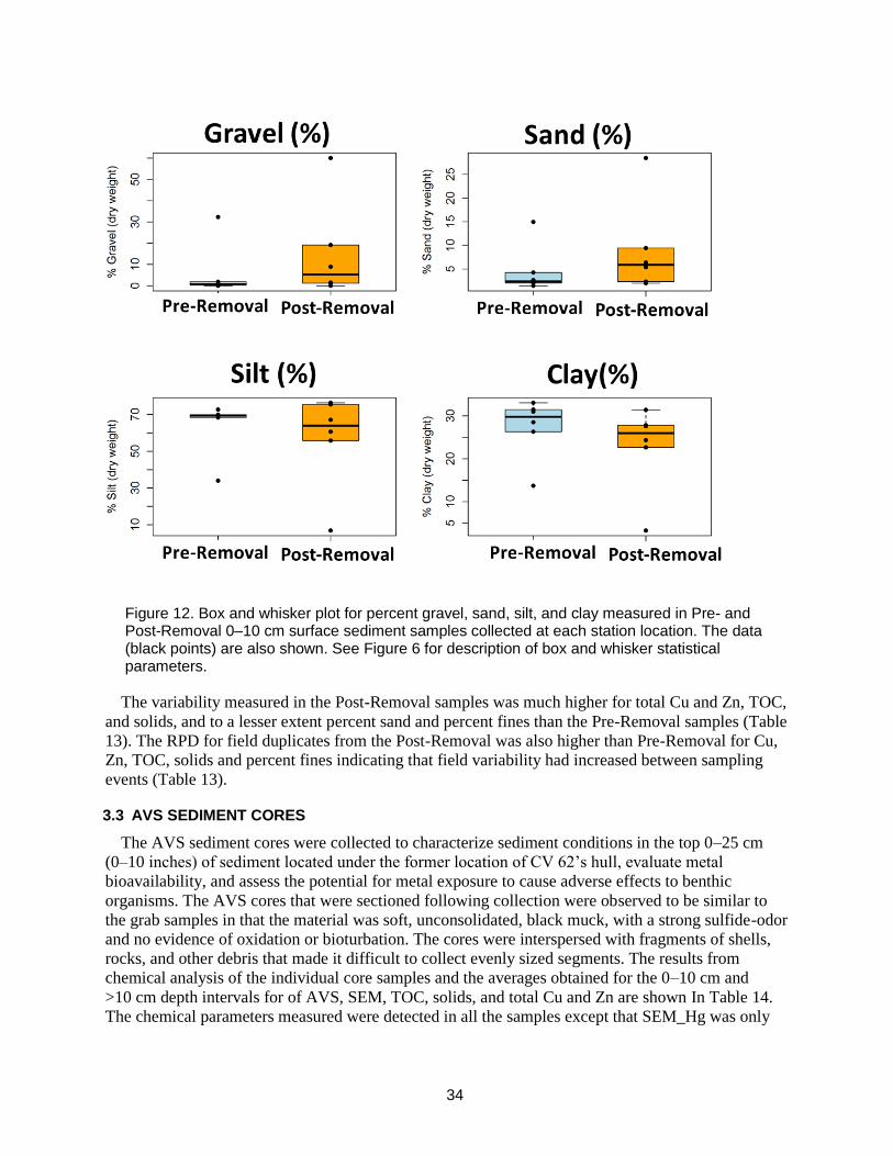
34

Figure 12. Box and whisker plot for percent gravel, sand, silt, and clay measured in Pre- and Post-Removal 0–10 cm surface sediment samples collected at each station location. The data (black points) are also shown. See Figure 6 for description of box and whisker statistical parameters.

The variability measured in the Post-Removal samples was much higher for total Cu and Zn, TOC,

and solids, and to a lesser extent percent sand and percent fines than the Pre-Removal samples (Table

13). The RPD for field duplicates from the Post-Removal was also higher than Pre-Removal for Cu,

Zn, TOC, solids and percent fines indicating that field variability had increased between sampling

events (Table 13).

3.3 AVS SEDIMENT CORES

The AVS sediment cores were collected to characterize sediment conditions in the top 0–25 cm

(0–10 inches) of sediment located under the former location of CV 62’s hull, evaluate metal

bioavailability, and assess the potential for metal exposure to cause adverse effects to benthic

organisms. The AVS cores that were sectioned following collection were observed to be similar to

the grab samples in that the material was soft, unconsolidated, black muck, with a strong sulfide-odor

and no evidence of oxidation or bioturbation. The cores were interspersed with fragments of shells,

rocks, and other debris that made it difficult to collect evenly sized segments. The results from

chemical analysis of the individual core samples and the averages obtained for the 0–10 cm and

>10 cm depth intervals for of AVS, SEM, TOC, solids, and total Cu and Zn are shown In Table 14.

The chemical parameters measured were detected in all the samples except that SEM_Hg was only

35

detected in two samples and AVS was not detected in 2 core sections sampled from station CV62-4

(Table 14)

The concentration of AVS ranged from not detected to 46 mol/g dry weight. The abundance of

SEM metals was: SEM_Zn > SEM_Cu > SEM_Pb >> SEM_Ni >> SEM_Cd >> SEM_Hg. The

SEM ranged from 2.12–29.07 mol/g dry weight. Most samples had higher AVS than SEM,

however, there were notable exceptions (see below) resulting in SEM – AVS > 0 for 8 out of the 23

samples (35%) analyzed (Table 14).

The TOC and Solids content in the core sections ranged from 0.5–4.5% and 18.5–83.9%,

respectively (Table 14). A trend of lower TOC for higher Solids was observed for the core sections

that was similar to the trend observed for the grab samples (Figure 13A). The TOC in the grab

samples increased with percent fines (Figure 13B), so it is reasonable to assume a similar relationship

between TOC and Fines in the core sections. Low TOC below 2% was measured in 3 of 23 (13%) of

the core sections, while high TOC > 3.5% was present in 8 of 23 (35%) of the samples. The Solids

content was also quite variable, about half of the samples had Solids < 25% indicating that most of

the samples were very watery and loosely consolidated. There was not a strong relationship between

TOC and AVS, however, AVS > 20 mol/g dry weight only occurred when TOC > 2.5% Figure

14A). There was not a similar relationship between TOC and SEM, as SEM appeared to be

independent of TOC (Figure 14B).

Figure 13. The relationship between TOC and solids in Pre- and Post- surface sediment samples and core sections (A) and TOC and Fines in the Pre- and Post- surface sediment samples (B).

36

Figure 14. The relationship between TOC and AVS (A) and TOC and SEM (B) measured in core sections.

37

There was also high variability in the total Cu and Zn measured in the core sections (Table 14).

Four of the core section samples exceeded the MCC for Cu, one sample exceeded the MCC for Zn

and one other sample exceeded the SQC for Zn.

The core profiles for TOC, Solids, total Cu and Zn, AVS and SEM, and the individual SEM

metals are plotted for each station in Figure 15–Figure 20. The core profiles for Station CV 62-1

(bow of ship) showed uniform distribution of TOC, Solids, total Cu, and total Zn with core depth

(Figure 15). The AVS was low at the surface of the core (0–3 cm, 0.1 mol/g dry weight), increased

to about 10 mol/g dry weight at 3–6 cm depth, decreased to 0.4 µmol/g dry weight for the 6–10 cm

section and then remained above 12 mol/g dry weight for the remainder of the core. The SEM

concentrations were relatively constant down core with the highest concentrations of SEM_Zn and

SEM_Cu measured in the 6–10 cm section Figure 15.

Figure 15. Core profiles for station CV62-1 showing the percent TOC and solids content (upper left panel), total Cu and Zn concentrations (upper right

panel), AVS and SEM concentrations (lower left panel), and the SEM metals (lower right panel).

38

The core collected from Station CV62-2 only penetrated 10 cm into the bottom due to the hard

substrate present at the site (Figure 16). The divers reported the presence of boulders, rip rap, and

other debris at this location which made it difficult to collect longer core samples. At this station

TOC and AVS were much higher and Solids were much lower in the surface section (0–5 cm), while

the lower section (5–10 cm) had much higher Solids content and lower TOC and AVS ((Figure 16).

The SEM was also highest in the lower core section where the SEM was dominated by SEM_Zn and

SEM_Pb ((Figure 16).

Figure 16. Core profiles for station CV62-2 showing the percent TOC and solids content

(upper left panel), total Cu and Zn concentrations (upper right panel), AVS and SEM concentrations (lower left panel), and the SEM metals (lower right panel).

39

The core profile from station CV62-3 was also limited in depth (0–14 cm, Figure 17). The TOC

(0.45%) was very low in the 0–5 cm surface section while Solids was high (84%). The 5–10 cm

section was very high for total Zn (7,400 g/g dry weight) and Cu (23,400 g/g dry weight) which

was reduced in the 10–14 cm section (Figure 17). The AVS was lower than the SEM metal in the 0–5

cm and 5–10 cm sections, but AVS increased to 45 mol/g dry weight, which was much higher than

SEM (5.6 mol/g dry weight). The SEM metals were dominated by high concentrations of

SEM_Zn that reached 17 and 21 mol/g dry weight in the top two core sections, respectively, while

SEM_Cu peaked at 7.3 mol/g dry weight in the 5–10 cm section (Figure 17).

Figure 17. Core profiles for station CV62-3 showing the percent TOC and solids content (upper left panel), total Cu and Zn concentrations (upper right

panel), AVS and SEM concentrations (lower left panel), and the SEM metals (lower right panel).

40

For Station CV62-4 (stern of the vessel) the surface TOC was about 2% and then remained at 3.2%

for the remainder of the core. Solids were higher at the surface (40%) but remained lower (18–26%)

for the rest of the core (Figure 18). Total Cu and Zn were below the sediment quality benchmarks,

while SEM metals, specifically SEM_Zn and SEM_Cu were elevated in the surface (0–3 cm) but

were relatively constant for the remainder of the core (Figure 18). The AVS was high at the surface

and bottom of the core, but was absent from the mid-core sections (Figure 18). The odd-looking AVS

profile may be an artifact if AVS were lost during sample processing (Figure 18).

Figure 18 Core profiles for station CV62-4 showing the percent TOC and solids content (upper left panel), total Cu and Zn concentrations (upper right panel),

AVS and SEM concentrations (lower left panel), and the SEM metals (lower right panel).

41

The core profiles for Station CV62-5 showed a total Cu spike of 1500 g/g dry weight in the 5–10

cm section (Figure 19). The AVS was higher than the SEM in all the cores sections, but AVS was

reduced to 8.7 mol/g dry weight in the 5–10 cm section (Figure 19). The 5–10 cm section was also

relatively elevated with SEM_Zn and SEM_Cu (3.4 and 2.5 mol/g dry weight, respectively, (Figure

19).



42

The core profile for Station CV62-6 (portside, forward midship) showed high total Cu (1,810 g/g

dry weight) and high SEM-Zn (16.3 mol/g dry weight) in the surface 0–5 cm section, but the AVS

was greater than SEM for all depth intervals (Figure 20). The SEM metals were dominated by

SEM_Zn which was highest in the surface segment, but decreased to 1.3 to 2.4 mol/g dry weight

down the core (Figure 20).



43

In general, there was a weak relationship between total Cu and Zn and SEM_Cu and SEM_Zn that

was driven by a few samples with very high concentrations of total metals that also had relatively

high SEM (Figure 21). On average the SEM_Cu accounted for about 30% (±20%) of the total Cu,

however, there were five samples in which the SEM_Zn was >> total Zn (Figure 21). This result is

unexpected because the total digestion should yield more metal than the AVS procedure. This may

be caused by inhomogeneity in the sample aliquots that were processed separately for the analysis.

The laboratory reported high inhomogeneity in duplicate samples from the AVS core sections (see

Appendix A-3. If the suspect samples with SEM_Zn >> total Zn are omitted, then SEM_Zn

accounted for about 30% (± 27%) of the total Zn present (Figure 21).

Figure 21. The relationship between total Cu and Zn (plotted on log scale) and the amount of

SEM_Cu and SEM_Zn (in g/g dry weight) measured in core sections collected Post-Removal. The regression lines for Cu (red) and Zn (blue) and the 1:1 ratio between SEM : Total Metal (dashed line) are also shown.

44

The sediment core data were pooled by depth to calculate the average concentrations of AVS in

the 0–10 cm and >10 cm intervals Table 14B). Based on the average concentrations, only Station

CV62-3 had SEM concentrations significantly higher than AVS concentrations in the top 0–10 cm

(Figure 22A) and all stations had AVS concentrations that were significantly higher than SEM

concentrations for depths > 10 cm (Figure 22B). When all the data are pooled by depth the average

AVS concentration exceeded SEM by about 5 and 25 mol/g dry weight for the 0–10 cm and > 10

cm depth intervals, respectively (Table 14B, Figure 23A). When total Cu and Zn were averaged by

depth, much higher concentrations of Cu and Zn were measured in the 0–10 cm surface layer (2,356

and 859 g/g dry weight for total Cu and Zn, respectively) than in the deeper > 10 cm layer (264 and

210 g/g dry weight for total Cu and Zn, respectively; Table 14B, Figure 23B).

Figure 22. The average AVS and SEM (error bars show standard deviation) measured in core sections from the top 0–10 cm (A) and >10 cm core depths (B) for each station.

45

Figure 23. The average (standard deviation) of AVS and SEM (A) and total Cu and Zn (B) concentrations measured by core depth.

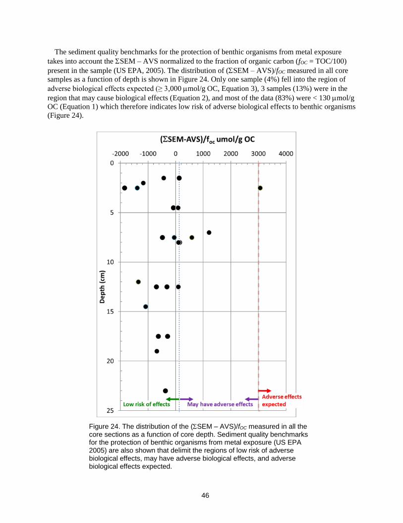
46

The sediment quality benchmarks for the protection of benthic organisms from metal exposure

takes into account the SEM – AVS normalized to the fraction of organic carbon (fOC = TOC/100)

present in the sample (US EPA, 2005). The distribution of (SEM – AVS)/fOC measured in all core

samples as a function of depth is shown in Figure 24. Only one sample (4%) fell into the region of

adverse biological effects expected (≥ 3,000 mol/g OC, Equation 3), 3 samples (13%) were in the

region that may cause biological effects (Equation 2), and most of the data (83%) were < 130 mol/g

OC (Equation 1) which therefore indicates low risk of adverse biological effects to benthic organisms

(Figure 24).

Figure 24. The distribution of the (SEM – AVS)/fOC measured in all the core sections as a function of core depth. Sediment quality benchmarks for the protection of benthic organisms from metal exposure (US EPA 2005) are also shown that delimit the regions of low risk of adverse biological effects, may have adverse biological effects, and adverse biological effects expected.

47

The probability of exceeding sediment quality benchmarks for the protection of benthic organisms

was calculated by pooling the sediment core data by depth, calculating the mean ( ) and standard

deviation ( ) for Y = (AVS-SEM)/foc, and estimating the probability of exceeding the benchmarks

using Equation 7 assuming a normal distribution and Equation 8 assuming a lognormal distribution

(Table 16). The probability of exceeding sediment quality benchmarks is shown graphically for the

0-5 cm depth interval in Figure 25. The probability density function was used to calculate the

probability of exceeding sediment quality benchmarks for the protection of benthic organisms from

metal exposure (US EPA, 2005) assuming the data fit a normal (Figure 25A) and lognormal (Figure

25B) distribution. The data points are also shown and the lognormal probability density function is

plotted on x-axis with back-transformed units (Figure 25C) to better visualize the data distribution

(although the units of probability density function are undefined for the back transformed

illustration). In the illustrations, the probability of exceeding the benchmark is the area under the

curve to the right of the benchmark (Figure 25) which was calculated directly from the cumulative

distribution functions in Equation 7 and Equation 8.

Based on average concentrations of metals and AVS measured in the 0–10 cm core sections and

using the most conservative assumptions, the analysis showed that there was a low (8.9%) chance of

possible impact, a medium chance (27.1%) of potential impact, and high chance (64%) of negligible

impact to the benthic community from metal toxicity (Table 16A). The calculations using the

lognormal distribution were slightly more conservative; there was a 9.5% chance for adverse effects

expected, a 21% chance for may have adverse effects, and a 70% chance for low risk of adverse

effects (Table 16B). The probability of adverse effects occurring decreased for the core segments

deeper in the core (Table 16). For the 0–10 cm surface layer, there was a 8.9% chance for adverse

effects expected, a 27% chance for may have adverse effects, and a 64% chance for low risk from

metal exposure at the site (Table 16B).

48

Table 16. The probability of (SEM – AVS)/fOC exceeding sediment quality benchmarks for the protection of benthic organisms from metal exposure (US EPA, 2005) for core data pooled by core depth and calculated assuming data conformed to a normal (A) and lognormal distribution (B). The

benchmarks define low risk of adverse biological effects (≤ 130 mol/g OC), may have adverse

biological effects (> 130 mol/g OC), and adverse biological effects expected (> 3000 mol/g OC).

Probability of

Core Depth BX Low Risk

May have Adverse

Effects BX

Adverse Effects

Expected

cm umol/g OC P(B130) 1-P(B130)-[1-P(B3000)] umol/g OC P(B3000) 1-P(B3000)

0-5 cm 130 0.5894 0.3938 3000 0.9832 0.0168

5-10 cm 130 0.4200 0.5800 3000 1.0000 0.0000

10-15 cm 130 0.9173 0.0827 3000 1.0000 0.0000

15-25 cm 130 0.9995 0.0005 3000 1.0000 0.0000

0-10 cm 130 0.5483 0.4460 3000 0.9943 0.0057

> 10 cm 130 0.9515 0.0485 3000 1.0000 0.0000

0-5 cm 3.3284 0.6988 0.2065 3.6990 0.9053 0.0947

5-10 cm 3.3284 0.4588 0.5406 3.6990 0.9994 0.0006

10-15 cm 3.3284 0.8825 0.1161 3.6990 0.9986 0.0014

15-25 cm 3.3284 0.9973 0.0027 3.6990 1.0000 0.0000

0-10 cm 3.3284 0.6404 0.2711 3.6990 0.9115 0.0885

> 10 cm 3.3284 0.9039 0.0960 3.6990 0.9999 0.0001

B. Lognormal Distribution

Probability of

A. Normal Distribution

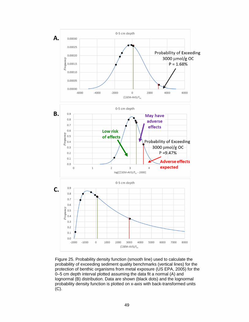
49

Figure 25. Probability density function (smooth line) used to calculate the probability of exceeding sediment quality benchmarks (vertical lines) for the protection of benthic organisms from metal exposure (US EPA, 2005) for the 0–5 cm depth interval plotted assuming the data fit a normal (A) and lognormal (B) distribution. Data are shown (black dots) and the lognormal probability density function is plotted on x-axis with back-transformed units (C).

50

3.4 MUSSEL TISSUES

Mussel tissues were sampled and analyzed for total Cu, total Zn, moisture, and lipid content to

provide a source term estimate of the Cu and Zn present in the biomass living on the hull prior to

biofouling removal. The data from the mussel tissue analysis are presented in Table 17 and plotted in

Figure 26. The concentration of Cu ranged from 19–30 g/g dry weight with a mean of 20 g/g dry

weight (CoefV* = 35%) and the concentration of Zn ranged from 129 -195 g/g dry weight with a

mean of 150 g/g dry weight (CoefV* = 19%, Table 17). The RPD for the field duplicates was less

than 10% for the metals on a dry weight basis (Table 17). The lipid and solid content were fairly

consistent among the samples with a CoefV* of 12% and 9% for lipid and solid content, respectively

(Table 17, Figure 26). A summary of benthic infauna measured in surface grabs collected near CV 62

prior to biofouling removal is shown in Table 18.

Table 17. Summary of total Cu and Zn, lipid, and solids measured in mussel (Mytilus spp.) tissue samples collected from the hull of CV 62 prior to biofouling removal.

Table 18. Summary of benthic infauna measured in surface grabs collected near CV 62 prior to biofouling removal.

Copper Zinc Copper Zinc Lipids Total Solids

Location ID Sample_ID Comment

CV62-Transect1 CV62MUS-01 11 specimens 3.27 24.80 19.24 145.88 2.1 17.0

CV62-Transect2 CV62MUS-02 12 specimens 3.16 26.30 15.49 128.92 2.1 20.4

CV62-Transect3 CV62MUS-03 average of Field Dups 5.25 34.05 28.97 188.30 1.7 18.1

CV62-Transect4&5 CV62MUS-05 13 specimens 2.59 23.80 14.97 137.57 1.9 17.3

average 3.57 27.24 19.67 150.17 1.94 18.20

standard deviation 1.16 4.66 6.49 26.35 0.21 1.54

CV* 34.6% 18.2% 35.0% 18.6% 11.7% 9.0%

CV62MUS-03 7 specimens 5.63 33.8 30.27 181.72 1.8 18.6

CV62MUS-04 7 specimens, Field Dup 4.87 34.3 27.67 194.89 1.5 17.6

RPD of Field Dup 14.5% 1.5% 9.0% 7.0% 18.2% 5.5%

CV62-Transect3

ug/g wet weight ug/g dry weight % wet weight

51

Figure 26. The concentration of total Cu (upper left panel), total Zn (upper right panel), percent lipid content (lower left panel), and percent solid content (lower right panel) measured in mussel tissues of specimens collected from Transect Belts during the biological survey of CV 62.

3.5 BENTHIC INFAUNA

Benthic infauna samples were collected to characterize the benthic community present at the site

prior to biofouling removal. The benthic census showed that very limited macro-invertebrates were

present at the site (Table 22). The extremely low abundance was expected given the highly anoxic

conditions of the sediment. No evidence of macro-invertebrate activity or bioturbation was observed

in the jelly-like muck collected with the Ponar sampler. The only biological activity observed in the

sample was the abundance of anoxic microbial organisms whose presence was attested by the strong

hydrogen sulfide odor and lack of visible oxidation in the samples.

3.6 HULL AND SEA FLOOR VIDEO SURVEY

The video taken by the PSNS&IMF Divers on March 30, 2017 was compared to the hull survey

videos of portions of the hull and bottom of CV 62 recorded by Seaward Marine Inc. prior to hull

cleaning in November 2016. The comparison showed that many organisms living on the hull had

survived the hull cleaning were still alive and living on sea floor below the location where CV 62

was berthed (Appendix C-1: Video Clips). Dense assemblages of barnacles (Balanus spp.), mussels

(Mytilus spp.), polychaete feather duster tube worms (Sabellidae and Serpulidae), large sea anemones

(Metridium senile) and many other invertebrates were documented growing on CV62’s hull (Earley

et al., 2017). The video of the sea floor taken about 8 weeks after biofouling removal showed that the

sea floor was covered with masses of tube worms, sea anemones, mussels, and other organisms from

the vessel that were still alive and functioning on the sea floor. In addition, many crabs (Cancer spp.)

52

and other opportunistic bottom feeders were observed foraging and feeding on the biological

material. Since the bottom consisted of soft mud with little substrate for epibenthic organisms the

material from the hull appeared to be providing substrate and habitat increasing the biodiversity and

abundance of the bottom community on the sea floor below CV62’s former berth (Appendix C-1:

Video Clips).

53

4. DISCUSSION

4.1 ANALYTICAL ACCURACY

The DQOs developed for this study (Table 1) were achieved by collecting sediment samples in the

zone of influence under CV 62 prior to biofouling removal and resampling the same area after

removal and towing of the vessel was complete. Additionally, sediment cores were collected and

analyzed to evaluate the potential metal bioavailability and toxicity at the site. The analytical

parameters selected for the study met the performance-based QA/QC for acceptability and usability,

discrepancies were documented in the lab reports, and validated data with data qualifiers, if

applicable, were used for the analysis.

The greatest source of error associated with the analytical results was the variation in the field

samples and inhomogeneity of samples collected at the same time and location (Field Duplicates and

Lab Duplicates). High variation in sediment samples collected near piers, pilings, and docking areas

have been reported by other studies within the BNC (US Navy, 2012; Wang et al., 2016; Kirtay et al.,

2017). This means that increasing the number of samples may not necessarily reduce the variability,

it would however, increase the degrees of freedom in statistical tests.

The analytical methods required to determine AVS from the sediment core sections are not

generally “routine” methods run by the contract lab, therefore, the laboratory was requested to run

additional LCS. The six repeated measurements of the same sample resulted in a CV* of 41% which

bounds the uncertainty that can be placed on the AVS results. In comparison to AVS, the results for

total and SEM metals were within the expected accuracy of 70–130% for all the results reported.

4.2 COMPARABLE STUDIES

Comparable studies were identified that reported similar parameters from locations in the vicinity

of Mooring G. The total Cu and Zn, grain size parameters, TOC, and Solids from this study (Table

19) were compared to data from the Washington State Department of Ecology's Urban Watershed

Initiative (UWI) that collected samples throughout the Bainbridge Basin in May 2009 including 6

stations within inner Sinclair Inlet (Figure 27; Weakland et al., 2013), Charleston Beach monitoring

conducted in May 2015 (Figure 28, URS Group 2016b), and LTM conducted for OUB Marine

(Figure 29; US Navy, 2012; URS Group, 2015 & 2016a). The LTM monitoring consists of

periodically collecting a composite of three 0-10 cm grabs from each 500 ft grid within OUB Marine

(Figure 4) and 1500 ft grid in outer Sinclair Inlet (Figure 30). During LTM sampling conducted in

October 2003 (Kohn, Miller, Brandenberger, and Johnston, 2004, 2008) and May 2010

(Brandenberger et al., in prep), the composite samples were split with the ENVVEST Monitoring

Program to obtain additional data on metals in the sediments of Sinclair Inlet (Table 29). There was a

general trend of increasing total Cu and Zn with increasing Fines and TOC in the samples (Figure

31). The Pre-Removal grab samples fell along the trend line, but three of the Post-Removal samples

for Cu and one of the Post-Removal samples for Zn were enriched and were well above the trend line

(Figure 31) indicating a source of metal other than that expected a function of grain size or TOC. In

comparison to the available studies, the highest total Cu and Zn concentrations were measured in

samples collected at Mooring G following biofouling removal (Post-Removal).

54

Table 19. Summary of sediment data collected near CV 62 for sampling conducted Pre- (A) and Post-Removal (B) of biofouling and data from comparable studies performed near the area reported from Ecology's Urban Waters Initiative (C), Charleston Beach monitoring (D), and long term monitoring for Operable Unit B conducted in 2003 (E and F) and 2010 (G and H).

55

Figure 27. Location of stations in Sinclair Inlet sampled by Ecology’s UWI project (Weakland et al., 2013) in May 2009 (red pins) and this study at Mooring G where CV 62 was formerly berthed (light blue spheres).

Historical data for total Cu, total Zn, AVS, and SEM is reported for a station sampled near

Mooring G (3a, Figure 29) are reported in Johnston (1993) and Chadwick et al. (1993) (Table 20),

and core profiles from age-dated cores from inner Sinclair Inlet are reported for Cu and Zn (Crecelius

et al., 2003; Brandenberger et al., 2008; Figure 32). These data show that there are relatively lower

metal concentrations near the surface of core that represents the most recent deposits. The down-core

concentrations of Cu and Zn peak during the latter half of the 20th Century, which corresponds to

core depths of about 15–30 cm (Brandenberger et al., 2008). The core profile representative of

Sinclair Inlet near Mooring G (S2, Figure 32) yielded a long-term average deposition rate of 0.35 ±

0.05 cm/yr and a surface mixing depth of 2.5 cm (Table 21, Brandenberger et al., 2008). At this

deposition rate it would take 28.5 (25–33) years to deposit 10 cm of sediment in this area of Sinclair

Inlet. This estimate is the long-term estimate for the area (S2, Figure 32) as a whole and neglects near

field inputs such as the raining of biogenic material from the hull, local runoff of particulates, and

disturbances from propeller wash and ship movements in the area. These data imply that since CV 62

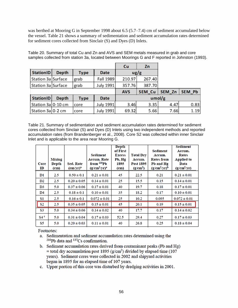
56

was berthed at Mooring G in September 1998 about 6.5 (5.7–7.4) cm of sediment accumulated below

the vessel. Table 21 shows a summary of sedimentation and sediment accumulation rates determined

for sediment cores collected from Sinclair (S) and Dyes (D) Inlets.

Table 20. Summary of total Cu and Zn and AVS and SEM metals measured in grab and core samples collected from station 3a, located between Moorings G and F reported in Johnston (1993).

Table 21. Summary of sedimentation and sediment accumulation rates determined for sediment cores collected from Sinclair (S) and Dyes (D) Inlets using two independent methods and reported accumulation rates (from Brandenberger et al., 2008). Core S2 was collected within inner Sinclair Inlet and is applicable to the area near Mooring G.

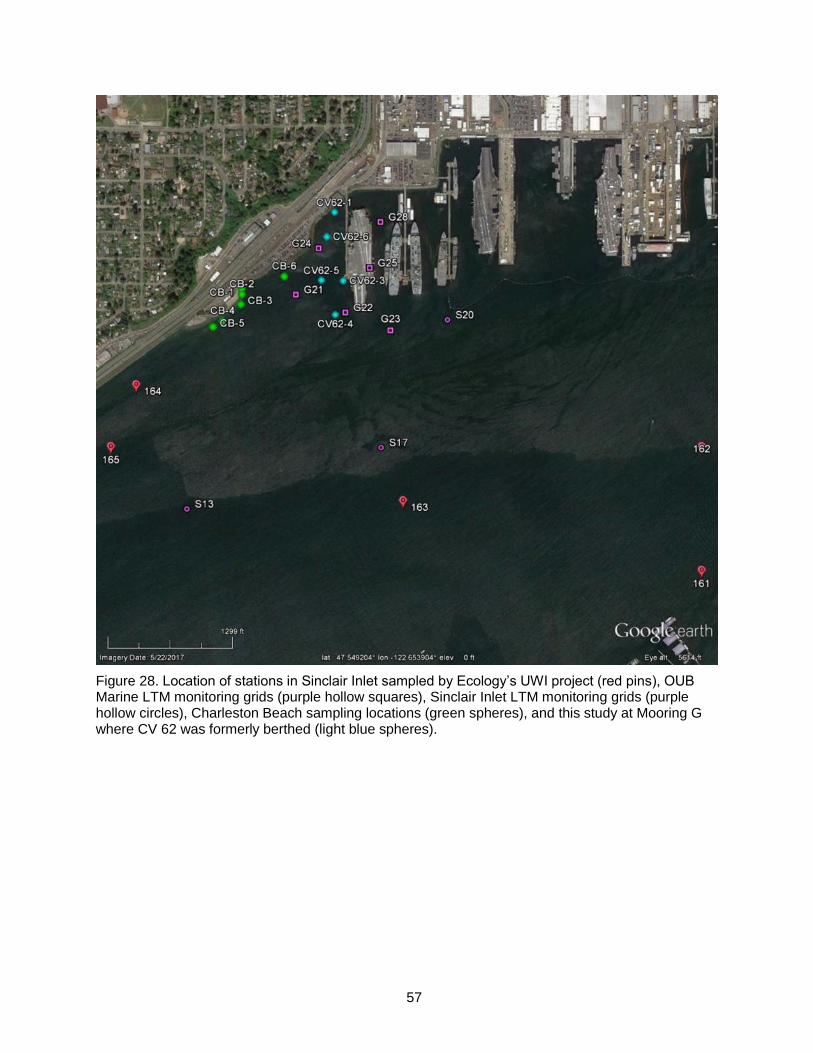
57

Figure 28. Location of stations in Sinclair Inlet sampled by Ecology’s UWI project (red pins), OUB Marine LTM monitoring grids (purple hollow squares), Sinclair Inlet LTM monitoring grids (purple hollow circles), Charleston Beach sampling locations (green spheres), and this study at Mooring G where CV 62 was formerly berthed (light blue spheres).

58

Figure 29. Location of stations near Mooring G sampled by Marine LTM monitoring grids (purple hollow squares), Charleston Beach sampling locations (green spheres), AVS-SEM sediment cores (orange hexagon [3a]), and this study where CV 62 was formerly berthed (light blue spheres).

59

Figure 30. Location of Mooring G and the 1500-ft sampling grids in outer Sinclair Inlet sampled as part of the LTM for OUB Marine (figure from US Navy 2012).

Figure 31. Relationship of Total Cu and Total Zn to percent fines (upper panels) and percent TOC measured in surface sediment samples from Pre- (blue squares) and Post-Removal (red circles) and comparable studies (black points) in Sinclair Inlet.

60

Figure 32. Age dated core profiles for total Cu and Zn measured from stations in Sinclair Inlet including station S2 located near Mooring G (Brandenberger et al., 2008).

The mussel tissue residues sampled from the hull of CV 62 were compared to the ENVVEST

Mussel Watch data collected from a network of stations within Sinclair and Dyes Inlets and the

passages connecting to the central basin of Puget Sound (Figure 33, and Figure 34; Johnston, 2017).

The ENVVEST mussel watch stations have been sampled semi-annually from 2010-2016; the

sampling includes a sample obtained from a local seafood market containing mussels harvested from

Penn Cove, WA. The mussels sampled from CV 62 were within the range of Cu and Zn

concentrations reported from other stations within Sinclair and Dyes Inlets (Figure 35) including

station PS01 at the base of Mooring G and stations SIGST and SIRP located within inner Sinclair

Inlet. The mussel tissue Cu concentrations from CV 62 were higher than the stations closest to

Mooring G, while the Zn concentrations from CV 62 were lower than the nearest stations. The

mussel tissue Cu and Zn concentrations were within the medium range of concentrations reported for

the National Mussel Watch Program (Kimbrough et al., 2008). On average, the concentrations of Cu

and Zn measured in mussels collected from the hull of CV 62 were at or below the Critical Body

61

Residue (CBR, (Figure 35) benchmark, below which effects from metal exposure to mussels are not

expected (Johnston et al., 2007; Applied Biomonitoring, 2009). In comparison to seafood samples

harvested from Penn Cove, WA (PKPLPC, Figure 35), mussel tissue concentrations from CV 62

were about twice as high for Cu and within the range of Zn concentrations measured in seafood

samples harvested from Penn Cove (Figure 35).

Figure 33. Location of ENVVEST mussel watch sampling stations sampled semiannually from 2010–2016 and the location of Penn Cove, WA where the seafood market samples were harvested.

62

Figure 34. Location of ENVVEST mussel watch sampling stations in Sinclair Inlet sampled semiannually from 2010–2016.

63

Figure 35. Comparison of the average (CV*) mussel tissue concentration of total Cu (upper panel) and Zn (lower panel) sampled from the hull of CV62, the ENVVEST mussel watch tissue concentrations sampled semi-annually from 2010–2016, and the range of tissue concentrations reported from the National Mussel Watch (MW) Program (Kimbrough, 2008).

The benthic community data collected during this study were also compared to other infaunal

studies conducted in Sinclair Inlet (Table 22; Weakland et al., 2013; Kirtay et. al., 2017). The

infaunal counts from Mooring G (stations CV62-1 to CV62-6) were extremely low compared to

abundance and number of taxa reported from the UWI study and Pier 7 activated carbon

demonstration project (Table 22). The samples from Mooring G were collected during the winter,

which would have much lower abundance than samples collected in spring and summer when

64

temperature and primary productivity levels are much higher. The lack of benthic diversity and

abundance in the sediment was contrasted by the very high abundance and diversity of the epibenthic

fouling community present on the hull of CV 62 as well as the nearby docks and pilings. The

biofouling removal essentially transferred the epibenthic community from the hull of CV 62 to the

sea floor, which greatly increased the abundance and diversity present. Prior to biofouling removal,

the biological material from the hull would rain down upon the bottom, as evidenced by the

abundance of shells and other debris present in the Pre-Removal samples. This process would occur

slowly, however the hull cleaning resulted in a mass transfer of organisms and substrate from the hull

to the sea floor where, it appears, the organism were able to re-establish themselves on the bottom

creating a new frontier for colonization (see Appendix C-1 Video Clips).

Table 22. Summary of sediment infauna data collected near CV 62 (A) prior to biofouling removal and sediment infauna data from comparable studies performed near the area reported from Ecology's Urban Waters Initiative (B) and the Pier 7 Activated Carbon Demo Project (C).

4.3 METAL BIOAVAILABILITY AND TOXICITY

Metal bioavailability and the potential for metal exposure to cause adverse effects to benthic

organisms were evaluated by collecting sediment cores from the site and conducting AVS and SEM

measurements of core sections in the top 0–25 cm (0–10 inches) of sediment located under the

former location of CV62’s hull. When all the data are pooled by depth, there is enough AVS present

to bind the SEM metals, reducing the risk of adverse effects (Figure 23) and the benchmark for

adverse effects from metal exposure (SEM - AVS)/fOC > 3,000 mol/g dry weight was only

exceeded by one sample (1/23 samples = 4%) during the study (Figure 24). However, there is

Individuals Taxon Abundance

StationID Depth Type Date # # #/m2

A. CV62 Pre Removal

CV62 0-10 cm grab 12/13/2016 8 7 13

B. Urban Waters Initiative (Weakland et al. 2013)

UWI-SI-160 0-3 cm grab May-2009 147 8 1470

UWI-SI-161 0-3 cm grab May-2009 87 8 870

UWI-SI-162 0-3 cm grab May-2009 392 31 3920

UWI-SI-163 0-3 cm grab May-2009 421 26 4210

UWI-SI-164 0-3 cm grab May-2009 560 39 5600

UWI-SI-165 0-3 cm grab May-2009 473 34 4730

C. Pier 7 Demo Project (Kirtay et al. 2017)

Pier 7 Cap* (n=10) 0-15 cm core Aug-2012 13.9 6554.2

Pier 7 Reference (n=4) 0-15 cm core Aug-2012 5.0 1685.3

Pier 7 Cap (n=10) 0-15 cm core Aug-2013 12.8 8077.7

Pier 7 Reference (n=4) 0-15 cm core Aug-2013 9.3 2777.8

Pier 7 Cap (n=10) 0-15 cm core Jul-2014 13.4 5855.5

Pier 7 Reference (n=4) 0-15 cm core Jul-2014 11.5 5638.8

Pier 7 Cap (n=10) 0-15 cm core Jul-2015 9.5 4699.7

Pier 7 Reference (n=4) 0-15 cm core Jul-2015 8.3 4027.8

*Baseline samples collected prior to amendment cap placement

65

uncertainty about this finding due to the variability and interferences associated with the method,

including analytical inaccuracy, seasonal variation of AVS, sample inhomogeneity, and other sources

of variation.

As discussed above, the analytical precision of the AVS measurement was about 41% of the “true

value” and there was uncertainty about how effective the laboratory was in controlling for the loss of

AVS in the samples by removing the oxidized layer prior to processing and preventing oxidation

during extraction. Overall the AVS analytical results met acceptable QA/QC criteria, however, the

AVS concentrations may have been under estimated because AVS was not detected in two samples,

and there were large variations in field and lab duplicates (Table 14).

The concentrations of AVS are known to vary in marine and estuarine sediments with maximum

values occurring during the warm summer months when sulfate reduction by marine bacteria are at

the highest levels and lowest during the winter when water column dissolved oxygen levels are near

saturation (Boothman and Helmsetter, 1992; Boothman et al., 2001; US EPA, 2005). Since the AVS

samples for this study were collected late winter/early spring (March 30, 2017), it is very likely that

the AVS concentrations were at or near minimum levels. The AVS concentrations during the summer

months can be much higher (Table 20; Johnston, 1993) while seasonal SEM would remain relatively

constant. Consequently, the additional AVS would afford more protection from metal exposure

during the warmer months when marine organisms are most active.

Inhomogeneity and variability in field sampling is an inherent component of studies conducted

within non-uniform environments such as active naval harbors with hardened shorelines, overwater

structures, vessel berthing, ship traffic, propeller wash, and other disturbances that can affect the

sedimentary environment (Johnston, 1993; Chadwick et al., 1993; Wang et al., 2016; Kirtay et al.,

2017). Therefore, the sediment results reported for this study should be considered a snap shot of the

heterogeneous environment present at the site.

There was a high amount of variability in the samples collected near Mooring G. The core profiles

obtained for each sampling station varied considerably in terms of sediment texture, contaminant

levels, and distribution of AVS and SEM (Table 13, Table 14, Figure 15–Figure 20). Concentrations

of total Cu did not exceed the WA State Sediment Management Standards (SMS) Maximum

Chemical Criteria (MCC) of 390 g/g dry weight in any of the Pre-Removal 0–10 cm grabs, three

(50%) of the Post-Removal 0–10 cm grabs exceeded Cu concentrations of 390 g/g dry weight

(Table 13), and 4 of 23 (17%) sediment core sections exceeded the Cu MCC benchmark (Table 14).

For Zn, only two samples exceeded the Zn MCC of 960 g/g dry weight, one sample from the Post-

Removal grabs (station CV62-4, Table 13) and the 5-10 cm section from the core collected at station

CV62-3 (Table 14). The SMS benchmarks are useful for determining the relative magnitude of

contamination present (Ecology, 2013). However, they are not very useful in predicting ecological

effects because the MCC values are based on apparent effects thresholds of a mixture of sediment

contaminants (Ginn and Pastorok, 1992), and do not represent a dose-response threshold for

individual sediment contaminants, as such as those that are available for water quality criteria

thresholds, for example.

Metal toxicity in sediments is controlled by geochemical processes that affect metal bioavailability

and toxicity, therefore, it is more appropriate to assess metal toxicity using the AVS benchmarks

derived based on (SEM - AVS)/fOC (US EPA, 2005). The AVS benchmarks only evaluate the

potential for metal toxicity through pore water exposure to free metal, the AVS benchmarks do not

address metal bioaccumulation or trophic transfer in the food web. Food-web biomagnification of

metals is not likely a major concern as marine invertebrates are well adapted for mediating Cu and

66

Zn since these metals are both micro-nutrients and essential to life at low levels and toxic at higher

levels, thus limiting biomagnification in the food web (Paquin et al., 2011).

The variation in concentrations of total Cu and Zn in the Pre-Removal samples was 18% and 42%,

respectively and this variance increased to 74% and 97% for the Post-Removal event, respectively.

Additionally, the variance in grain size parameters for Fines, TOC, and Solids increased by at least a

factor of two between the two sampling events (Table 13). This indicates that the biofouling removal

caused a disturbance in the sea floor conditions. However, it is unclear whether the disturbance also


present. Because the bottom consists of soft muds, the material falling from the ship would not

necessarily remain on the surface but would “splash” on the bottom sinking into the muck and

disturbing the bottom conditions. Additionally, diving operations during the cleaning and other

operations required to prepare the ship for towing may have also contributed to disturbance.

Under the anoxic conditions, the metal contaminants present would most likely be inert, bound up

in insoluble metal sulfides. Whether the disturbance will contribute to the release of contamination

depends on the rate of sediment reworking and oxidation. For example, if sediments are recolonized

by benthic organisms, they might release metals and other contaminants that were previously

sequestered at the site. However, if sulfides remain higher than the metals then any effect from metal

exposure would be minimized. Even if the upper sediments are reworked and oxidized there will still

remain a large pool of AVS that will serve as a sink (or source) of metals at the site (Johnston, 1993).

4.4 SEA FLOOR BOTTOM COMMUNITY

As seen in the video clips of the sea floor, the masses of tube worms, mussels, and anemones

evidently increased the structure and diversity of the bottom community that attracted crabs and other

bottom feeders. Prior to biofouling removal, the bottom below the ship was essentially a biological

desert, except for the anoxic bacteria that dominated the benthic environment. In contrast, the

biofouling community living on the hull was a highly abundant and diverse community (Earley et al.,

2018a).

The shells and other calcareous material from the hull cleaning evolution served as substrate for

attachment space which was quite limited on the pre-existing unconsolidated sediment. Some of the

species in the community transferred from the hull to the sea floor were filter and suspension feeders

that need substrate to remain above the mud. This community also consisted of invertebrate

predators, grazers, omnivores and scavengers including an abundance of polychaetes that included

both selective and non-selective deposit feeders. The latter produce volumes of rejected fecal matter

such as feces, also known as castings. The castings contain unharvested organic matter and bacteria

which are a rich food source for other consumers. Whether this community remains viable over time

was outside the scope of this study, however, the video surveys clearly showed that many of the

organisms remained viable for at least two months after cleaning and were still functioning on the sea

floor where the hull cleaning occurred.

4.5 OUTCOME FOR DECISION MATRIX

The decision matrix was used to summarize the evaluation based on the difference between the

Pre- and Post-Removal 0-10 cm sediment grabs and the potential for adverse biological effects from

metal exposure estimated from the AVS core sections collected at the site (Table 23). There were no

statistically significant differences (p ≤ 0.05) detected for any of the sediment parameters measured

Pre- and Post-Removal for both parametric (normal and lognormal) and non-parametric statistical

tests (Table 15). The lack of statistical significance between the two sampling periods was due to the

high variability for both sampling periods. There was a statistically significant difference for total Zn

67

at the p ≤ 0.10 significance level, with Zn concentration about 1.8 times higher in the Post- samples.

Based on metal bioavailability and toxicity estimated from the AVS cores there was a low (9%)

chance of possible impact, a medium chance (27%) of potential impact, and high chance (64%) of

negligible impact (Table 23).

Table 23. Outcome of the decision matrix based on the evaluation of sediment data collected Pre- and Post-Removal and the chance of metal bioavailability causing adverse biological effects determined from sediment cores after CV 62 was removed Sinclair Inlet.

≤ 130 umol/g OC130 umol/g OC > and

≤3000 umol/g OC > 3000 umol/g OC

Low Risk of

Adverse

Biological Effects

May have Adverse

Biological Effects

Adverse

Biological Effects

May be Expected

None

Cu, Gravel, Sand,

Silt, Clay, TOC,

Solids (p≥0.05)

Slightly DifferentHigh Chance of

Negligible Impact

Medium Chance of

Potential Impact

Low Chance of

Probable Impact

Zn (p = 0.078) 64.0% 27.1% 8.9%

>2x and <5x Pre-Removal

≥5x and <10x Pre-Removal

≥10x Pre-Removal

Metal Bioavailability In Sediment

(SEM-AVS)/f OC

Magnitude of Difference

Stat

isti

cal D

iffe

ren

ce f

rom

Bas

eli

ne

No Difference or Better

than Pre-Removal

≤2x Pre-Removal

68

This page left blank intentionally.

69

5. SUMMARY AND CONCLUSIONS

The data developed for this study provided a basis for (1) determining whether biofouling removal

from the ex-INDEPENDENCE (CV62) impacted sediment quality at Mooring G and (2) assessing

the nature and extent of any impact. The before and after total Cu and Zn data were evaluated to

determine whether any increase chemical contamination could be attributed to biofouling removal.

Furthermore, the potential bioavailability and toxicity of metals were evaluated by measuring AVS,

SEM, moisture, and TOC from the core sections obtained from the site after CV 62 was removed

from Sinclair Inlet.

Sediment chemistry sampling was performed at six locations within the zone of influence near the

ship prior to the start of operations (Pre-Removal) and approximately one month after the ship was

moved from Sinclair Inlet and about two months after hull cleaning was completed (Post-Removal).

Surface sediment chemistry samples were collected by ponar grab for the Pre-Removal samples and

with divers for Post-Removal samples. The surface sediment samples (0–10 cm) were composited

and analyzed for total Cu, total Zn, grain size, Solids, and TOC. During the Post-Removal sampling

event, sediment cores (0–25 cm) were also collected from each station to obtain samples for analysis

of AVS and SEM, total Cu and Zn, Solids, and TOC to evaluate metal bioavailability and toxicity at

the site.

During the Pre-Removal sampling event, benthic community samples were also collected by ponar

grab at the six sediment sampling stations. The benthic community samples were sieved through a 1

mm sieve, preserved with formalin, and submitted for benthic community analysis.

Mussel tissues were sampled from the hull of CV 62 and analyzed for total Cu, total Zn, moisture,

and lipid content to provide a source term estimate of the Cu and Zn present in the biomass living on

the hull prior to biofouling removal.

Underwater video of the sea floor obtained during the post project sampling by the PSNS&IMF

Divers on March 30, 2017 was compared to the hull survey videos of portions of the hull and bottom

of CV 62 recorded by Seaward Marine Inc. prior to hull cleaning in November 2016. The

comparison showed that many organisms living on the hull had survived the hull cleaning were still

alive and living on the sea floor below the location where CV 62 was berthed (Appendix C-1 Video

Clips).

Data from the sediment surface samples (0–10 cm) taken before and after biofouling removal of

project show that there were no statistically significantly (p ≤ 0.05) differences in concentrations of

total Cu , grain size, and TOC. However, total Zn concentrations were significantly different at the p

≤ 0.10 level, and were about twice as high as concentrations prior to biofouling removal. In addition,

data from the sediment cores for AVS, SEM, and TOC were used to assess the bioavailability and

potential toxic effects of metals by comparing the (SEM – AVS)/fOC measured to benchmarks of

adverse biological effects from metal toxicity to the benthic community developed by US EPA

(2005). Based on average concentrations of metals and AVS measured in the 0–10 cm core sections

and using the most conservative assumptions, the analysis showed that there was a low (8.9%)

chance of possible impact, a medium chance (27.1%) of potential impact, and high chance (64%) of

negligible impact to the benthic community from metal toxicity. This finding suggests that the

potential impact on the benthic community from metal exposure associated with biofouling removal

was low.

The concentrations of total Cu and Zn measured in mussel tissues sampled from the hull of CV 62

prior to cleaning were within the range of mussel tissue concentrations reported for mussel watch

stations within Sinclair and Dyes Inlets. The benthic census showed very limited macro-invertebrates

70

were present at the site prior to cleaning, however the video of the sea floor taken about 8 weeks after

biofouling removal showed that the sea floor was covered with masses of tube worms, sea anemones,

mussels, and other organisms from the vessel that were still alive and functioning on the sea floor. In

addition, many crabs and other opportunistic bottom feeders were observed foraging and feeding on

the biological material.

The findings from this study showed that the potential impact of biofouling removal to the benthic

community from the release of copper and zinc was low and that the benthic community in the area

of the vessel was not adversely degraded. However, it is unclear whether the disturbance also


present. As seen in the video clips of the sea floor, the masses of tube worms, mussels, and anemones

evidently increased the structure and diversity of the bottom community that attracted crabs and other

bottom feeders. Under the anoxic conditions, the metal contaminants present would most likely be

inert, bound up in insoluble metal sulfides. Whether the disturbance will contribute to the release of

contamination depends on the rate of sediment reworking and oxidation. The findings from this study

showed that the potential impact of biofouling removal to the benthic community from the release of

copper and zinc was low and that the benthic community in the area of the vessel was not adversely

degraded.

71

REFERENCES

Allen, H.E, G. Fu, W. Boothman, D.M. DiToro, and J.D. Mahony. 1991. “Draft analytical method

for determination of acid volatile sulfide in sediment,” December 1991, U.S. EPA Office of

Water, EPA-821-R-91-100.

Allen, H. E., Fu, G., and Deng, B. 1993. “Analysis of acid-volatile sulfide (AVS) and simultaneously

extracted metals (SEM) for the estimation of potential toxicity in aquatic sediments,”

Environmental Toxicology and Chemistry (12)1441–1453.

Applied Biomonitoring. 2009. “Using Caged Mussels to Characterize Exposure & Effects over Small

Spatial Scales in Sinclair Inlet: A Risk Assessment Based Approach. A Caged Mussel Study for

Puget Sound Naval Shipyard & Intermediate Maintenance Facility Project ENVVEST” Final

Report. Available online at

https://drive.google.com/file/d/0B2b5tj0gsZXVYXY1blVrSzF4RDA/edit?usp=sharing

Boothman, WS, Helmstetter A. 1992. “Vertical and seasonal variability of acid volatile sulfides in

marine sediments. Research Report. Environmental Monitoring and Assessment Program,” U.S.

Environmental Protection Agency, Narragansett, RI.

Boothman, WS, Hansen DJ, Berry WJ, Robson D, Helmstetter A, Corbin J, Pratt SD. 2001.

“Variation of acid volatile sulfides and metals and biological response in field-exposed

sediments,” Environmental Toxicology and Chemistry Journal, (20):264-272.

Brandenberger J. M., E.A. Crecelius, and R. K. Johnston. 2008. “Draft Contaminant Mass Balance

for Sinclair and Dyes Inlets, Puget Sound, Washington,” Prepared for the Puget Sound Naval

Shipyard and Intermediate Maintenance Facility Project ENVVEST Bremerton, Washington

under Contract DE-AC06-76RLO 1830, Pacific Northwest National Laboratory, Richland,

Washington.

Brandenberger, J.M., G.A. Gill, R.K. Johnston, G. Rosen and J. Guerrero, (in Prep). “Sediment

Quality Verification Study and Baseline for Process Improvement for Puget Sound Naval

Shipyard & Intermediate Maintenance Facility,” Bremerton, WA. Pacific Northwest National

Laboratory, Marine Sciences Laboratory, Sequim, WA.

Chadwick, D. B., Lieberman, S. H., Reimers, C. E., Young, D. 1993. “An Evaluation of Contaminant

Flux Rates from Sediments of Sinclair Inlet, WA, Using a Benthic Flux Sampling Device,”

Naval Command Control and Ocean Surveillance Center RDTE Div San Diego, Ca. Available

online at http://www.dtic.mil/cgi-

bin/GetTRDoc?Location=U2&doc=GetTRDoc.pdf&AD=ADA277484

Crecelius, E., R.K. Johnston, M. Miller, J. Brandenberger, J. Leather and J. Guerrero. 2003.

“Contaminant Mass Balance for Sinclair and Dyes Inlets, Puget Sound,” WA. Paper presented at

Georgia Basin Puget Sound Research Conference, Vancouver, BC, Canada, April 2, 2003.

Available online at

http://archives.eopugetsound.org/conf/2003GBPS_ResearchConference/PAPERS/ORAL/6e_crec

e.pdf.

Diefenderfer, H.L., G.E. Johnson, R.M. Thom, K.E. Buenau, L.A. Weitkamp, C.M. Woodley, A.B.

Borde, R.K. Kropp. 2016. “Evidence-based evaluation of the cumulative effects of ecosystem

restoration.” Ecosphere Volume 7 (pp. 3). Available online at

http://onlinelibrary.wiley.com/doi/10.1002/ecs2.1242/abstract.

https://drive.google.com/file/d/0B2b5tj0gsZXVYXY1blVrSzF4RDA/edit?usp=sharing

http://www.dtic.mil/cgi-bin/GetTRDoc?Location=U2&doc=GetTRDoc.pdf&AD=ADA277484

http://www.dtic.mil/cgi-bin/GetTRDoc?Location=U2&doc=GetTRDoc.pdf&AD=ADA277484

http://archives.eopugetsound.org/conf/2003GBPS_ResearchConference/PAPERS/ORAL/6e_crece.pdf

http://archives.eopugetsound.org/conf/2003GBPS_ResearchConference/PAPERS/ORAL/6e_crece.pdf

http://onlinelibrary.wiley.com/doi/10.1002/ecs2.1242/abstract

72

Dutch, M., V. Partridge, S. Weakland, K. Welch, and E. Long. 2009. “Quality Assurance Project

Plan: The Puget Sound Assessment and Monitoring Program Sediment Monitoring Component,”

Washington State Department of Ecology Publication, 98 pp. Available online at

https://fortress.wa.gov/ecy/publications/SummaryPages/0903121.html.

Dutch, M., V. Partridge, S. Weakland, K. Welch, and E. Long. 2015. “Addendum 7 to Quality

Assurance Project Plan, The Puget Sound Assessment and Monitoring Program: Sediment

Monitoring Component,” Monitoring in the Bainbridge Basin. Washington State Department of

Ecology Publication 15-03-118, 23 pp.

Earley, P.J., L.A. Bolick, D.E. Marx, I. Rivera-Duarte, R.K. Johnston, N.C. Dickenson, J.S.

Krumholz. 2018a. “Comprehensive Field Surveys and Evaluation of Biofouling and Coating

System on the Hull of the ex-USS INDEPENDENCE (CV62),” Technical Report 3081. Space

and Naval Warfare Systems Center Pacific, San Diego, CA, 83pp.

Earley, P.J., I. Rivera-Duarte, R.K. Johnston, L.A. Bolick, D.E. Marx, N.C. Dickenson, J.S.

Krumholz, 2018b. “Water Quality Monitoring of Biofouling Removal from the Ex-

Independence,” Technical Report. Space and Naval Warfare Systems Center Pacific, San Diego,

CA.

Ecology (Washington Department of). 2013. “Sediment Management Standards,” Chapter 173–204

WAC, Publications number 13-09-055, February 2013, 151pp. Available online at

https://fortress.wa.gov/ecy/publications/SummaryPages/1309055.html

Ecology. 2015. “Puget Sound Estuary Protocols. Publication No. 15-09-046,” Washington State

Department of Ecology, March 2015, Lacey, WA. Available online at


Ecology. 2017. “How to Submit Data to EIM (for public users)” (formerly EIM Submittal

Guidelines). Version 3.0. Washington State Department of Ecology, November 2017.

https://fortress.wa.gov/ecy/eimhelp/HelpDocuments/OpenDocument/14

ENVVEST. 2006. “Puget Sound Naval Shipyard and Intermediate Maintenance Facility Project

ENVVEST Community Update CD: Study Plans, Reports, Data and Supporting Information,”

Washington State Department of Ecology Publication Number 06-10-054. Prepared by Space and

Naval Warfare Systems Center San Diego, Marine Environmental Support Office - NW,

Bremerton, WA. August 2006. http://www.mesodat.org/Public/ENVVEST2006/

Ginn, T.C. and R.A. Pastorok. 1992. “Assessment and management of contaminated sediments in

Puget Sound,” In Sediment Toxicity Assessment, G. Allen Burton, Jr. (ed), Lewis Publishers,

Boca Raton, FL, pp. 371–401.

Johnston, R.K, 1993. Acid Volatile Sulfides and Simultaneously Extracted Copper, Lead, and Zinc in

Sediments of Sinclair Inlet, Washington. Naval Command Control and Ocean Surveillance

Center RDT&E Division Technical Report 1552, San Diego, CA, 90 pp. Available online at

www.dtic.mil/cgi-bin/GetTRDoc?AD=ADA284406.

Johnston, R.K., D.E. Leisle, J. M. Brandenberger, S.A. Steinert, M. Salazar, and S. Salazar. 2007.

“Contaminant Residues in Demersal Fish, Invetebrates, and Deployed Mussels in Selected Areas

of the Puget Sound.” WA. Proceedings of the 2007 Georgia Basin Puget Sound Research

Conference, Puget Sound Action Team and Environment Canada. Vancouver, BC, Canada,

March 26–29, 2007. Available online at

http://depts.washington.edu/uwconf/2007psgb/2007proceedings/papers/13e_johns.pdf.




https://fortress.wa.gov/ecy/eimhelp/HelpDocuments/OpenDocument/14

http://www.mesodat.org/Public/ENVVEST2006/

http://depts.washington.edu/uwconf/2007psgb/2007proceedings/papers/13e_johns.pdf

73

Johnston, R.K., J. Brandenberger, Li-Jung Kuo, C. Suslick, E. Mollerstuen, E. Beckley. 2014.

“Mussel Watch monitoring to assess status, tends, and continuous process improvement of

environmental protection and restoration initiatives for Sinclair and Dyes Inlets, Liberty Bay, and

Port Orchard, Rich and Agate Passages of the Puget Sound.” WA. Proceedings of the 2014

Salish Sea Ecosystems Conference, April 30 – May 2, 2014, Seattle, WA. Available online at

https://event.crowdcompass.com/ssec2014/activity/kmuGu3CxPZ.

Johnston, R.K., W.R. Munns, P.L. Tyler, K. Finkelstein, K. Munney, P. Whittemore, F.T. Short, A.

Mellvile, and S. Hahn. 2002. “Weighing the Evidence of Ecological Risk of Chemical

Contamination in the Estuarine Environment Adjacent to the Portsmouth Naval Shipyard,”

Kittery, Maine, USA. Environmental Toxicology and Chemistry Volume 21, No. 1, pp 182-194.

Johnston, R.K. 2017. “ENVVEST "Mussel Watch Project: Monitoring Environmental Quality in

Local Waters. Presentation for All Ports Meeting, Brownsville,” WA, Jan 23, 2017.

Kimbrough, K. L., W. E. Johnson, G. G. Lauenstein, J. D. Christensen and D. A. Apeti. 2008. “An

Assessment of Two Decades of Contaminant Monitoring in the Nation’s Coastal Zone,” Silver

Spring, MD. NOAA Technical Memorandum NOS NCCOS 74. 105 pp. Available online at

http://ccma.nos.noaa.gov/publications/MWTwoDecades.pdf

Kirtay, V., G. Rosen, M. Colvin, J. Guerrero, L. Hsu, E. Arias, R. Johnston, B. Chadwick, M.

Grover, J. Arblaster, V. Magar, J. Conder, R. Webb, J. Collins, J. Germano, and A. Conrad.

2017. “Demonstration of In Situ Treatment with Reactive Amendments for Contaminated

Sediments in Active DoD Harbors,” Final Report: ESTCP Project ER-201131, January 2017,

884pp. Available online at https://www.serdp-estcp.org/Program-Areas/Environmental-

Restoration/Contaminated-Sediments/ER-201131/ER-201131-FR/(modified)/30Mar2017

Kohn, NP, MC Miller, JM Brandenberger, and RK Johnston. 2004. “Metals Verification Study for

Sinclair and Dyes Inlet,” Washington. Prepared for Puget Sound Naval Shipyard & Intermediate

Maintenance Facility Project ENVVEST, Bremerton, Washington. September, 2004. PNNL-

14872. Pacific Northwest National Laboratory, Richland, Washington.

Kohn, N.P., J.M Brandenberger, and R.K. Johnston. 2008. “Summary Report Metals and PAH

Verification Study for Sinclair Inlet,” Washington. Prepared for PSNS&IMF Project ENVVEST.

September 2008.

Morse, J. W., Millero, F. J., Cornwell, J. C. and Rickard, D. 1987. “The chemistry of the hydrogen

sulfide and iron sulfide systems in natural waters,” Earth Science Review. 24:1-42.

NAVSEA (Naval Sea Systems Command). 2006. “Naval Ships' Technical Manual, Chapter 081,

Waterborne Underwater Hull Cleaning of Navy Ships,” (S9086-CQ-STM-010, Revision 5).

NOAA NMFS. 2016. Letter of Aug 5, 2016 from Dona S. Wieting, National Oceanic and

Atmospheric Administration (NOAA) National Marine Fisheries Service (NMFS) to Mr.

William Boozer, Naval Sea Systems Command (NAVSEA) Inactive Ships Office (SEA-21I), Re:

Request for informal consultation under section 7(a)(2) of the Endangered Species Act and

Magnuson-Stevens Fishery Conservation and Management Act Essential Fish Habitat Response

regarding United States Navy Naval Sea Systems Command Inactive Ships Office proposed

contracted towing and dismantling of inactive U.S. Navy vessel ex-INDEPENDENCE.

Paquin, P., A. Redman, A. Ryan, and R. Santore. 2011. “Modeling the Physiology and Toxicology of

Metals. Fish Physiology,” 31. 429-484. 10.1016/S1546-5098(11)31031-X. Available online at

http://www.sciencedirect.com/science/article/pii/S154650981131031X

https://event.crowdcompass.com/ssec2014/activity/kmuGu3CxPZ

http://ccma.nos.noaa.gov/publications/MWTwoDecades.pdf

https://www.serdp-estcp.org/Program-Areas/Environmental-Restoration/Contaminated-Sediments/ER-201131/ER-201131-FR/(modified)/30Mar2017

https://www.serdp-estcp.org/Program-Areas/Environmental-Restoration/Contaminated-Sediments/ER-201131/ER-201131-FR/(modified)/30Mar2017

http://www.sciencedirect.com/science/article/pii/S154650981131031X

74

Puget Sound Estuary Program (PSEP). 1997. “Recommended Guidelines for Sampling Marine

Sediments, Water Column and Tissue in Puget Sound.” Prepared for U.S. Environmental

Protection Agency, Region 10, and Puget Sound Water Quality Action Team. April 21 1997. (see

Ecology 2015)

Sokal, R.R. and F.J. Rohlf. 1995. “Biometry: The principles and practice of statistics in biological

research.” Third Edition, W.H Freeham and Company, New York, NY, 887 pp.

SSC-PACIFIC and NUWC. 2016. “Project Work Plan for Monitoring Biofouling Removal from the

ex-INDEPENDENCE (CV62) Moored in Sinclair Inlet, Puget Sound,” WA. Prepared by Space

and Naval Warfare Systems Center Pacific and Naval Underwater Warfare Systems Center

Newport Division for Naval Sea Systems Command, Washington, DC. As Revised 1/23/2017

SSC-PACIFIC and NUWC 2017. “Comprehensive Field Surveys and Evaluation of Biofouling and

Coating System on the Hull of the ex-USS INDEPENDENCE (CV62),” Prepared by Space and

Naval Warfare Systems Center Pacific and Naval Underwater Warfare Systems Center Newport

Division for Naval Sea Systems Command, Washington, DC. As Revised June 2017.

Thom, R.M., G. Williams, A. Borde, J. Southard, S. Sargeant, D. Woodruff, J.C. Laufle, and S.

Glasoe. 2005. “Adaptively addressing uncertainty in estuarine and near coastal restoration

projects,” Journal of Coastal Research (40):94–108.

US EPA. 1994. Method 7470A (SW-846): Mercury in Liquid Waste (Manual Cold-Vapor

Technique). Revision 1. Washington , DC.

US EPA. 2005. “Procedures for the Derivation of Equilibrium Partitioning Sediment Benchmarks

(ESBs) for the Protection of Benthic Organisms: Metal Mixtures (Cadmium, Copper, Lead,

Nickel, Silver and Zinc).” EPA-600-R-02-011. Office of Research and Development.

Washington, DC 20460. Available online at https://clu-

in.org/conf/tio/porewater1/resources/EPA-ESB-Procedures-metals.pdf.

US Navy, US EPA, and Washington State Department of Ecology. 2000. Project ENVVEST: Phase I

Final Project Agreement for the Puget Sound Naval Shipyard, September 25, 2000 [Federal

Register: October 23, 2000 (Volume 65, Number 205)]. Available online at

https://archive.epa.gov/projectxl/web/pdf/fpasigned.pdf.

US Navy, 2012. “Third Five-Year Review,” Bremerton Naval Complex, Bremerton, WA.

https://semspub.epa.gov/work/10/676795.pdf.

URI (University of Rhode Island) 2006. “Chemistry 112, Solubility Product Constants near 25 C.”

Available online at http://bilbo.chm.uri.edu/CHM112/tables/KspTable.htm

URS Group, Inc. 2016a. “Final 2014 Operable Unit B Marine Phase 1 Long-term Monitoring

Report,” Bremerton Naval Complex, Bremerton, Washington. Prepared by URS for Naval

Facilities Engineering Command, Northwest, under Contract N44255-09 -D-4001. March 10,

2016.

URS Group, Inc. 2016b. “Final 2014 Operable Unit B Marine Phase 2 Long-Term Monitoring

Report PSNS Superfund Site Bremerton Naval Complex Bremerton,” Washington. Prepared for

Naval Facilities Engineering Command Northwest, U.S. Navy Contract No. N44255-09-D-4001,

Delivery Order 0087, 82pp. Available online at https://semspub.epa.gov/work/10/100034328.pdf.

https://clu-in.org/conf/tio/porewater1/resources/EPA-ESB-Procedures-metals.pdf

https://clu-in.org/conf/tio/porewater1/resources/EPA-ESB-Procedures-metals.pdf

https://archive.epa.gov/projectxl/web/pdf/fpasigned.pdf

https://semspub.epa.gov/work/10/676795.pdf

http://bilbo.chm.uri.edu/CHM112/tables/KspTable.htm

https://semspub.epa.gov/work/10/100034328.pdf

75

Wang, P., I. Rivera-Duarte, K. Richter, Q. Liao, K. Farley, H. Chen, J. Germano, K. Markillie, and J.

Gailani. 2016. “Evaluation of Resuspension from Propeller Wash in DoD Harbors.” ESTCP

Project ER-201031 Technical Report, Space And Naval Warfare Systems Center Pacific, San

Diego, CA, September 2016, 331pp. Available online at

http://www.dtic.mil/docs/citations/AD1030182

Weakland, S., V. Partridge, M. Dutch, E. Long, and K. Welch. 2013. “Sediment Quality in the

Bainbridge Basin, Changes from 1998 to 2009.” Washington State Department of Ecology

Publication 13-03-010. Available online at

https://fortress.wa.gov/ecy/publications/SummaryPages/1303010.html.

http://www.dtic.mil/docs/citations/AD1030182


77

BIBLIOGRAPHY

Brandenberger, J.M., G. Gill, R.K. Johnston, J. Guerrero, J. Leather, G. Rosen, B. Beckwith, and J.

Young. 2011. “Sampling and Analysis Plan for Sediment Quality Verification (SQV) Study and

Baseline for Process Improvement, Sinclair and Dyes Inlets, Puget Sound, Washington,”

Prepared for Puget Sound Naval Shipyard & Immediate Maintenance Facility Project

ENVVEST, Bremerton, WA. April 2011. SQV Sampling and Analysis Plan.

Labiosa, W., W. Landis, T. Quinn, R. Johnston, K. Currens, S. Redmond, and R. Anderson. 2014.

“Puget Sound Pressures Assessment Methodology. Puget Sound Partnership Technical Report

2014-02.” Tacoma, WA. Available online at

https://sites.google.com/site/pressureassessment/documents/PSPA%20MethodologyTech%20Me

mo%20Labiosa%20et%20al%202014%20FINAL.pdf?attredirects=0&d=1.

NIST (National Institute of Standards and Technology). 2017. SRM 2702 – “Inorganics in Marine

Sediment.” Available online at https://www-s.nist.gov/srmors/view_detail.cfm?srm=2702

https://sites.google.com/site/pressureassessment/documents/PSPA%20MethodologyTech%20Memo%20Labiosa%20et%20al%202014%20FINAL.pdf?attredirects=0&d=1

https://sites.google.com/site/pressureassessment/documents/PSPA%20MethodologyTech%20Memo%20Labiosa%20et%20al%202014%20FINAL.pdf?attredirects=0&d=1

https://www-s.nist.gov/srmors/view_detail.cfm?srm=2702

78


A-1

APPENDIX A RAW DATA REPORTS FROM ALS GLOBAL, KELSO, WA

APPENDIX A.1 ALS GLOBAL DATA REPORT FOR SEDIMENT GRABS PRE-REMOVAL

Appendices\A1_ALS-1_K1705946_Sed_Grabs_Pre.pdf

APPENDIX A.2 ALS GLOBAL DATA REPORT FOR SEDIMENT GRABS POST-REMOVAL

Appendices\A2_ALS-2_K1705817_Sed_Grabs_Post.pdf

APPENDIX A.3 ALS GLOBAL DATA REPORT FOR AVS CORES

Appendices\A3_ALS-3_K1705808_AVS_Cores.pdf

APPENDIX A.4 ALS GLOBAL DATA REPORT FOR MUSSEL TISSUES

Appendices\A4_ALS-4_K1705945_Mussel_Tissues.pdf

Note: For printed versions of the report there is a CD included that contains content shown here as

hyperlinks on the CD.

This page intentionally left blank

B-1

APPENDIX B TAXONOMIC DATA REPORT FROM ECOANALYST, MOSCOW, ID

B.1 BENTHIC DATA REPORT

Appendices\B_Apdx_Benthic_Data_Report.pdf



C-1

APPENDIX C VIDEO SURVEY RESULTS

C.1 VIDEO CLIPS

Video Clips of CV 62 Hull and Keel Prior to Cleaning and Sea Floor Adjacent to Mooring

G After CV 62 was Towed from Sinclair Inlet.

Appendices\C_^FOUO_CV62_Hull&Keel_SeaFloor_long_Annotated3.avi

Transcript of Video: Appendices\C_Video_Transcript.pdf



C-2

This page intentionally left blank

D-1

APPENDIX D ELECTRONIC DATA DELIVERABLE (EED) FORMATTED DATA

REQUIRED FOR SUBMISSION TO ECOLOGY’S ENVIRONMENTAL INFORMATION MANAGEMENT (EIM) SYSTEM

D.1 OVERVIEW

Appendix D contains three Excel files containing electronic data deliverable for study, location,

and Results

Study: Appendices\AppendixD\AppendixD_StudyDetails.xlsx

Location: Appendices\AppendixD\AppendixD_LocationDetails.xlsx

Results: Appendices\AppendixD\AppendixD_Results.xlsx



INITIAL DISTRIBUTION

84300 Library (1)

85300 Archive/Stock (1)

71760 R. K. Johnston (1)

71750 E Arias (1)

71760 D. E. Marx, JR. (1)

71750 P. J. Earley (1)

Defense Technical Information Center

Fort Belvoir, VA 22060–6218 (1)

5f. WORK UNIT NUMBER

REPORT DOCUMENTATION PAGE Form Approved

OMB No. 0704-01-0188

The public reporting burden for this collection of information is estimated to average 1 hour per response, including the time for reviewing instructions, searching existing data sources, gathering and maintaining the data needed, and completing and reviewing the collection of information. Send comments regarding this burden estimate or any other aspect of this collection of information, including suggestions for reducing the burden to Department of Defense, Washington Headquarters Services Directorate for Information Operations and Reports (0704-0188), 1215 Jefferson Davis Highway, Suite 1204, Arlington VA 22202-4302. Respondents should be aware that notwithstanding any other provision of law, no person shall be subject to any penalty for failing to comply with a collection of information if it does not display a currently valid OMB control number.

1. REPORT DATE (DD-MM-YYYY) 2. REPORT TYPE 3. DATES COVERED (From - To)

4. TITLE AND SUBTITLE 5a. CONTRACT NUMBER

5b. GRANT NUMBER

5c. PROGRAM ELEMENT NUMBER

5d. PROJECT NUMBER

5e. TASK NUMBER

7. PERFORMING ORGANIZATION NAME(S) AND ADDRESS(ES)

10. SPONSOR/MONITOR’S ACRONYM(S)

14. ABSTRACT

15. SUBJECT TERMS

16. SECURITY CLASSIFICATION OF:

a. REPORT b. ABSTRACT c. THIS PAGE 17. LIMITATION OF ABSTRACT

18. NUMBER OF PAGES

19a. NAME OF RESPONSIBLE PERSON

19B. TELEPHONE NUMBER (Include area code)

Standard Form 298 (Rev. 10/17) Prescribed by ANSI Std. Z39.18

PLEASE DO NOT RETURN YOUR FORM TO THE ABOVE ADDRESS.

6. AUTHORS

8. PERFORMING ORGANIZATION

REPORT NUMBER

11. SPONSOR/MONITOR’S REPORT NUMBER(S)

9. SPONSORING/MONITORING AGENCY NAME(S) AND ADDRESS(ES)

12. DISTRIBUTION/AVAILABILITY STATEMENT

13. SUPPLEMENTARY NOTES

SEPTEMBER 2018 Final

Biofouling Removal from the ex-INDEPENDENCE (CV 62) Moored in

Sinclair Inlet, Puget Sound, WA:


Robert K. Johnston

Ernie Arias

Donald E. Marx, Jr.


Patrick J. Earley

SSC-Pacific

53560 Hull Street

San Diego, CA 92152–5001 TR 3167

NAVSEA, SEA 211


Water Body Number

WA-15-0040 Sinclair Inlet

The ex-INDEPENDENCE (CV 62), which had been moored at Mooring G at Naval Base Kitsap in Bremerton, WA (NBK-BREM) since

decommissioning in September 1998 was towed on March 11, 2017 to Brownsville, TX, where the ship arrived on June 1, 2017 for dismantling.

Based on a consultation with National Oceanic and Atmospheric Administration (NOAA) National Marine Fisheries Service (NMFS), the Navy

was required to clean the ship's hull prior to towing in order to mitigate the possibility of transferring invasive species to other regions and

thereby harm endangered species and habitats. This report presents the sediment sampling and analysis results to assess potential impacts to

sediment quality from biofouling removal from CV 62 while it was moored at NBK-BREM and the Puget Sound Naval Shipyard & Intermediate

Maintenance Facility (PSNS&IMF) in Sinclair Inlet, Puget Sound, WA. The data developed for this study provided a basis for

1- determining whether biofouling removal from CV 62 impacted sediment quality at Mooring G and

2- assessing the nature and extent of any impact.

The findings from this study showed that the potential impact of biofouling removal to the benthic community from the release of copper and

zinc was low and that the benthic community in the area of the vessel was not adversely degraded.

Hull Cleaning; CV-62; USS Independence; Sediment analysis; biofouling removal; sediment impact assessment

U U U U 110

Patrick J. Earley

(619) 553-2768

NAVSEA Inactive Ships Program

1333 Isaac Hull Avenue,

SE Washington Navy Yard, DC 20376