biogeochemical validation of an interannual simulation of ... · southeast pacific. revista peruana...

159

Biogeochemical validation of an interannual simulation of the ROMS-PISCES coupled model

Rev. peru. biol. 23(2): 159 - 168 (August 2016)

Biogeochemical validation of an interannual simulation of the ROMS-PISCES coupled model in the Southeast Pacific

Dante Espinoza-Morriberon 1*, Vincent Echevin 2, Jorge Tam 1, Jesús Ledesma 1, Ricardo Oliveros-Ramos 1, Jorge Ramos 1 and Carlos Y. Romero 1,3

Validación biogeoquímica de una simulación interanual del modelo acoplado ROMS-PISCES en el Pacífico Sudeste

(1) Instituto del Mar del Perú , E sq . G amarra y V alle s/ n, Apartado 22, C allao, Perú .(2) L aboratoire d’ Océ anographie et de C limatologie: E xpé rimentation et Analyse Numé riq ue (L OC E AN), Institut Pierre-Simon L aplace (IPSL ), U PMC / C NRS/IRD/ MNH N, 4 Place Ju ssieu, C ase 100, 7 5252 Paris cedex 05, F rance.(3) U niversidad Nacional de Ingenierí a, F acultad de C iencias, Av. T ú pac Amaru 210, Rí mac, L ima* C orresponding authorE mail Dante E spinoza-Morriberon: despinoza@ imarpe.gob.peE mail V incent E chevin: vincent.echevin@ locean-ipsl.upmc.frE mail Jo rge T am: j tam@ imarpe.gob.peE mail Je sú s L edesma: j ledesma@ imarpe.gob.peE mail Ricardo Oliveros-Ramos: ricardo.oliveros@ gmail.comE mail Jo rge Ramos: j ramos@ imarpe.gob.peE mail C arlos Y . Romero: cromero@ imarpe.gob.pe

T RAB AJO S ORIG INAL E S

© L os autores. E ste artí culo es publicado por la Revista Peruana de B iologí a de la F acultad de C iencias B ioló gicas, U niversidad Nacional Mayor de San Marcos. E ste es un artí culo de acceso abierto, distribuido baj o los té rminos de la L icencia C reative C ommons Atribució n-NoC omercial-C ompartirIgual 4 .0 Internacional.(http:/ / creativecommons.org/ licenses/ by-nc-sa/ 4 .0/ ), q ue permite el uso no comercial, distribució n y reproducció n en cualq uier medio, siempre q ue la obra original sea debidamente citadas. Para uso comercial, por favor pó ngase en contacto con editor.revperubiol@ gmail.com.

Revista peruana de biologí a 23(2): 159 - 168 (2016)doi: http:/ / dx.doi.org/ 10.15381/ rpb.v23i2.124 27

ISSN-L 1561-0837Facultad de Ciencias Biológicas UNMSM

Journal home page: http:/ / revistasinvestigacion.unmsm.edu.pe/ index.php/ rpb/ index

Citación:E spinoza-Morriberon D., V . E chevin, J. T am, J. L edesma, R. Oliveros-Ramos, J. Ramos and C .Y . Romero. 2016. B iogeochemical validation of an interannual simulation of the ROMS-PISC E S coupled model in the Southeast Pacific. Revista peruana de biología 23(2): 159 - 168 (Agosto 2016). doi: http:/ / dx.doi.org/ 10.15381/ rpb.v23i2.124 27

Fuentes de financiamiento: JEAI EMACEP (Ecología Marina Cuantitativa del Ecosistema de Aflo-ramiento Peruano) y L MI DISC OH (Dinamica de Sistema de C orriente de H umboldt).

Información sobre los autores: DE M redactó el trabaj o y analizó los datos. V E y ROR analizaron los datos. JT M redactó el trabaj o. JL R y JR F ayudaron en la recolecció n de datos. C RT contribuyó en la discusió n en el trabaj o. Los autores no incurren en conflictos de intereses.

Presentado: 31/ 07 / 2015Aceptado: 08/ 06/ 2016 Publicado online: 27 / 08/ 2016

AbstractC urrently biogeochemical models are used to understand and q uantify ke y biogeochemical processes in the ocean. T he ob-jective of the present study was to validate predictive ability of a regional configuration of the PISCES biogeochemical model on main biogeochemical variables in H umboldt C urrent L arge Marine E cosystem (H C L ME ). T he statistical indicators used to evaluate the model were the bias, root-mean-square error, correlation coefficient and, graphically, the Taylor’s diagram. The results show ed that the model reproduces the dynamics of the main biogeochemical variables (chlorophyll, dissolved oxygen and nutrients); in particular, the impact of E l Niñ o 1997 -1998 in the chlorophyll (decrease) and oxygen minimum zone depth (increase). H ow ever, it is necessary to carry out sensitivity studies of the PISC E S model w ith different ke y parameters values to obtain a more accurate representation of the properties of the Ocean.

Keywords: PISC E S model; H C L ME ; chlorophyll; dissolved oxygen; nutrients.

Resumen Los modelos biogeoquímicos en la actualidad son utilizados para entender y cuantificar los principales procesos biogeo-q uí micos q ue suceden en el océ ano. E l obj etivo del presente estudio es validar estadí sticamente la habilidad predictiva de una simulació n del modelo biogeoq uí mico PISC E S en reproducir la diná mica de las principales variables biogeoq uí micas del E cosistema de la C orriente de H umboldt (E C H ). Para evaluar el modelo se utilizaron indicadores estadí sticos: sesgo, error de la raíz del cuadrado medio, coeficiente de correlación y gráficamente el diagrama de Taylor. Los resultados muestran que el modelo es capaz de reproducir la dinámica de las principales variables biogeoquímicas (clorofila, oxígeno disuelto y nutriente), captando bien el impacto que tiene El Niño 1997-1998 en la clorofila (disminución) y profundidad de la zona mí nima de oxí geno (incremento). E s necesario llevar a cabo estudios de sensibilidad del modelo PISC E S usando diferentes valores de los principales pará metros para obtener una mej or representació n de las propiedades biogeoq uí micas del océ ano.

Palabras claves: modelo PISCES; ECH; clorofila; oxígeno disuelto; nutrientes.

160

Espinoza-Morriberon et al.

Rev. peru. biol. 23(2): 159 - 168 (Agosto 2016)

IntroductionOceanographic models are used to study several ocean

processes (i.e. Kelvin waves impacts, coastal upwelling) and, in recent years, biogeochemical models have been developed to understand, quantify and predict the main biogeochemical processes and the complex dynamics between nutrients and plankton. In addition, biogeochemical models are coupled or used as forcings for High Trophic Level (HTL) models, aiming to understand ecosystem dynamics.

Intermediate complexity biogeochemical models, like NPZD type models, simulate the interaction between nitrate, phyto-plankton, zooplankton and detritus (Edwards 2001, Heinle & Slawig 2013). More complex biogeochemical models like PISCES model (Aumont & Bopp 2006) or BioEBUS model (Gutknecht et al. 2013) include more variables and processes, simulating a more complete representation of the ocean bio-geochemistry and plankton dynamics.

Biogeochemical models have been used in previous studies in Humboldt Current Large Marine Ecosystem (HCLME) in order to understand the climatological processes a�ecting the Oxygen Minimum Zone (OMZ) (Montes et al. 2014) and the climatological (Echevin et al. 2008, Albert et al. 2010) and interannual (Echevin et al. 2014) variability of phytoplankton and nutrients.

In the present study, we used statistical metrics to assess the skill of the coupled hydrodynamic and biogeochemical ROMS-PISCES model using data from surveys, remote sensing and international databases.

We analyzed the climatological and interannual (1992 ‒ 2008) biogeochemical variability, including the impact of El Niño 1997 ‒ 1998 event on the chlorophyll concentration and depth of the OMZ.

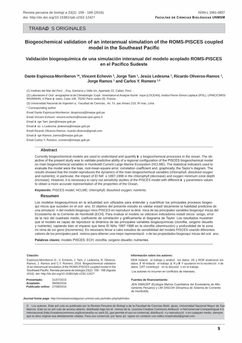
Material and methodsStudy area.- �e study area comprised the HCLME (0ºS

− 40ºS and 70ºW − 100ºW). To validate the biogeochemical model, two zones were de�ned: a) the area o� Peru within 200 km and between 06°S − 16°S; b) the area o� Chile within 200 km and between 30°S − 40°S (Fig. 1). �e seasons were de�ned as follows: summer (January − March), autumn (April − June), winter (July − September) and spring (October − December).

PISCES biogeochemical model.- �e PISCES biogeoche-mical model (Pelagic Interaction Scheme for Carbon and Ecosystem Studies) simulates marine biological productivity and describes biogeochemical cycles like carbon and major nutrients in the ocean (Aumont & Bopp 2006). PISCES model assumes that phytoplankton growth depends on ex-ternal concentration of nutrients and that the main nutrients in the medium follow the Red�eld ratio (C:N:P ~106:16:1)(Red�eld et al 1963). PISCES has 24 state variables, such as: nutrients (Phosphorus, Nitrogen, Silica and Iron), dissolved oxygen, two types of detritus (large and small), two classes of zooplankton (microzooplankton and mesozooplankton) and two classes of phytoplankton (nanophytoplankton and diatoms) (Fig. 2). Diatoms di�er from nanophytoplankton in their requirements of silicates, an increased consumption of iron and higher levels of nutrient saturation due to its larger size (Echevin et al. 2008).

Model con�guration.- In the present study the PISCES model is coupled to the hydrodynamical model ROMS (Re-gional Ocean Modeling System) (Shchepetkin & McWilliams 2005), following the coupling principles of Gruber et al. (2006), who coupled ROMS to a simpler biogeochemical model than PISCES. �e physical model ROMS has been used in several previous works to simulated the dynamics of the HCLME (Pen-ven et al. 2005, Colas et al. 2008, Montes et al. 2010, Echevin et al. 2012, Illig et al. 2014).

Our simulation covered a larger area to the north (10ºN) than the HCLME to reproduce more accurately the equatorial circula-tion, because surface and subsurface equatorial currents can a�ect the dynamics (Montes et al. 2010), oxygenation and productivity (Espinoza-Morriberón 2012) of Peruvian waters. �e model spa-tial resolution was 1/6º with 32 sigma vertical levels (which follow the topography of the ocean �oor), the output simulations were recorded of every averaged 6 days from 1992 to 2008.

Atmospheric forcings were obtained from two sources: (1) merging climatological SCOW data (Risien & Chelton 2008) with NCEP anomalies (www.ncep.noaa.gov/) for wind �elds and, (2) merging COADS climatology data (Da Silva et al. 1994) with NCEP anomalies for the heat �uxes and air tem-peratures. For boundary conditions the outputs of the global ORCA2-PISCES physical-biogeochemical coupled model (Aumont & Bopp 2006) were used. More details about model con�guration are described in Echevin et al. (2010, 2012) and Cambon et al. (2013).

Model ValidationData to validate the model.- To verify that the PISCES

model represents the main spatial patterns of biogeochemical variables in the HCLME (i.e. depth of the OMZ, nutrients and

Figure 1. C oastal zone betw een 0-200 km (grey) and zones for analyzing the behavior of the modeled variables off Peru and C hile.

161



surface chlorophyll), the following climatologies and interannual time series were used (Table 1):

Chemical. Oxygen and nutrients climatologies were ob-tained from CSIRO Atlas of Regional Seas "CARS 2009" (Ridgway et al. 2002) at a spatial resolution of 1/2º and a vertical resolution of every 5 m depth (from 0 − 200 m) and every 100 m depth (from 200 − 1000 m). Monthly series from 1992 to 2008 of the depth of the upper limit of the OMZ were obtained by merging the database of the Instituto del Mar del Peru (IMARPE) and the international database of WOD09 (García et al. 2010), following the methodology developed by Musial et al. (2011); the reader is referred to Bertrand et al. (2011) for more details about oxygen data processing.

Biological. Surface chlorophyll climatological and inte-rannual time series was obtained from the database of the Sea-viewing Wide Field-of-view Sensor (SeaWiFS) (Behren-feld & Falkowski 1997) at a spatial resolution of 1/12º and a monthly temporal resolution from 1997 to 2008.

All observed time series were interpolated on the model temporal resolution using the Laplace transformation method implemented in the FERRET program (http://ferret.pmel.noaa.gov/Ferret) to make comparisons between model and observations.

Data analysis.- Goodness of �t between observed and simu-lated data was measured using the following statistical indicators (Vichi and Masina 2009, Lehmann et al. 2009):

Bias (S), which re�ects the overestimation (positive) or un-derestimation (negative) of a simulation:

S = 1/n ∑(M – O) ……………(Eq.1)

Where n represents the number of pairs between observed (O) and modeled (M) data by time each bin. However it is necessary to keep in mind that positive and negative deviations in the model tend to cancel, so that the bias would represent the persistence of a di�erence between the modeled (M) and observed (O) values.

Root mean square error (RMSE), re�ects whether the mo-deled values di�er in magnitude from the observed values, so that a small RMSE would indicate good agreement between modeled and observed values:

RMSE= √((∑(M – O)^2 )/n)……………(Eq.2)

Correlation coe�cient, allows us to assess how strongly the temporal variations of the modeled and the observed values are related:

ρ(M,O)= cov(M,O)/(σM σO )……………(Eq.3)

Where cov (M, O) is the covariance between the time series of M and O, and σM σO are the standard deviations of M and O respectively.

In addition, Taylor diagrams (Taylor 2001) were used to evaluate the goodness of �t of the model: 1) between areas (o� Peru and Chile), and 2) between temporal variations (climato-logical and interannual). Taylor diagram integrates the RMSE, the correlation coe�cient and the standard deviation in a single diagram, to compare the �elds that are tested (coming from one or more models) and a reference �eld (representing the "truth" or the observed �eld).

Results and discussionSurface chlorophyll.- SeaWIFS interannual satellite data

(1997-2008) were interpolated on the model spatial resolution

ATMOSPHERE Air-ocean exchange

OXYGENAdvectionPhotosyntesis

Respiration

Microzoo

Mesozoo

POMDOM

Ammonium

Ocean

Nitrate

Iron

Silicate

Phosphate

Nanophyto

Diatoms

Rem

iner

aliz

atio

n

SEDIMENT

Nitr

ifica

tion

Figure 2. PISC E S model architecture. T he ecosystem model is show n omitting the carbonate system. T he grey arrows indicate the processes that influence the concentration of oxygen (modified from Aumont & Bopp 2006).

162



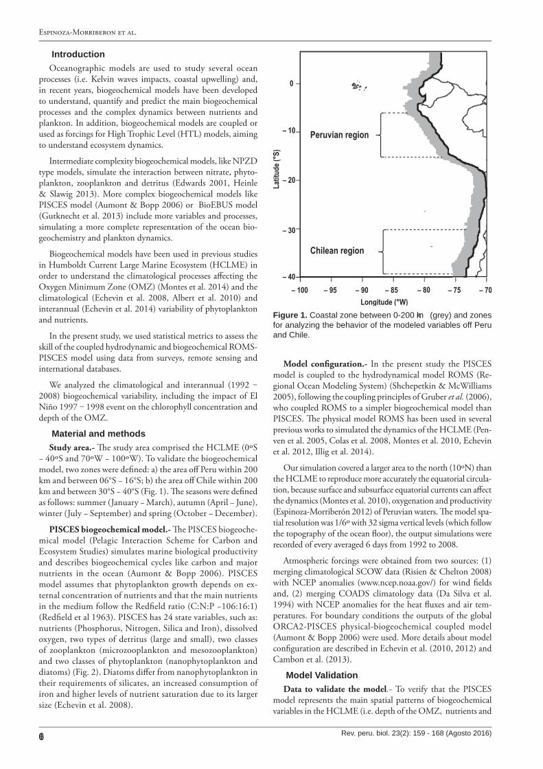
(~18 km) and the climatologies (for satellite and simulated data) were calculated between the years 2000-2008 to reduce the e�ect of the strong 1997-98 "El Niño". Figure 3 (a and b) shows that the simulation represents adequately the average spatial distribution of surface chlorophyll observed, reproducing larger chlorophyll values near the coast. In addition, the area of greatest productivity of the HCLME (Northern Central Peru) and the simulated distribution of the 1 mg Chl/m3 isoline, used as a proxy to de�ne the upwelling area (Nixon & �omas 2001), follows the annual pattern observed in SeaWiFS data. �e high productivity observed o� the Northern Center Peruvian region could be generated by the widening of the continental shelf in this area, which would provide a high amount of iron to the water column. �e iron is generally a key limiting element for phytoplankton (Bruland et al. 2005).

Goodness of �t indicators validated the model within the study area: within 200 km of the coast in Peruvian area, mean values of RMSE around 3.2 mg Chl/m3 and a mean positive bias of ~+2.5 mg Chl/m3 (Fig. 3c and 3d) were observed; fur-thermore, in the whole modelling region RMSE values mainly �uctuated between 0 at 0.5 mg Chl/m3 and bias values between -0.1 to 0.1 mg Chl/m3. �e overestimation of the simulations compared to the observed pattern could be in�uenced by the presence of clouds near the coast o� Peru that could have mas-ked some phytoplankton blooms. Another explanation for the model overestimation would be the lack of two-way coupling between PISCES and high trophic level model (to connect large zooplankton to top predators), which could in�uence phytoplankton mortality (Traver & Shin 2010). Also, a slightly positive bias was observed in the equatorial upwelling, which

MODELED VARIABLE OBSERVED DATA VALIDATION AREA

OMZ depthClimatology CARS (Ridgway et al., 2002) Peru, Chile

Interannual IMARPE (Graco, com.pers.) Peru

Surface chlorophyllClimatology SeaWIFS (Behrenfeld and Falkowski, 1997) Peru, Chile

Interannual SeaWIFS (Behrenfeld and Falkowski, 1997) Peru, Chile

Surface nutrients Climatology CARS (Ridgway et al., 2002) Peru, Chile

Table 1. Modeled variables in PISC E S and observed data bases used in the present study.

Figure 3. C omparison of the observed and modeled surface chlorophyll. Annual average of the modeled surface chloro-phyll (a) and SeaW IF S (b) in mg C hl/ m3 w ith the isoline of 1 mg C hl/ m3. Map of RMSE va-lues (c) and bias (d) calculated betw een PISC E S model and SeaW IF S surface chlorophyll a for the period simulation.

163



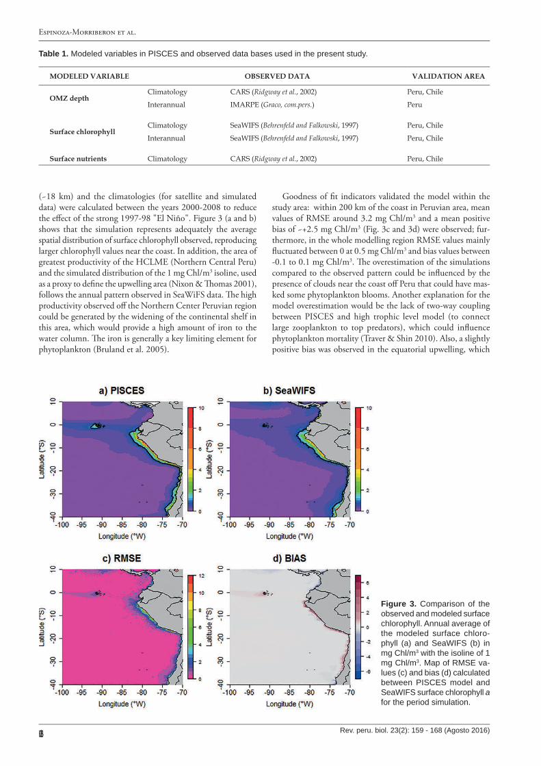
Figure 4. B ox diagrams of the modeled annual cycle of sur-face chlorophyll (grey) and SeaW iF S (w hite) off Peru (a) and C hile (b) region.

has also been observed by Albert et al. (2010), possibly because the model overestimate the equatorial upwelling.

�e annual cycle of surface chlorophyll within 200 km was acceptably reproduced by the model o� the coasts of Peru and Chile compared to the SeaWiFS data (from here, satellite values will be given in parentheses). Seasonality o� Peru had larger amplitude than in Chile. �e mean seasonal chlorophyll con-

centration presented highest values o� Peru during the summer and autumn months with 3.5 (3.2) mg Chl/m3 and lower values during winter with 2.5 (1.2) mg Chl/m3, while o� Chile, highest values were observed during spring and summer with 1.2 (1.5) mg Chl/m3 and lower values during winter with 0.9 (0.92) mg Chl/m3 (Fig. 4). Within the coastal area o� Peru, overestima-tion of simulations compared to SeaWIFS was also observed by Echevin et al. (2008) during all climatological months (~+1 mg Chl/m3) and by Albert et al. (2010) especially during winter, who mentioned that it could be due to the reduced availability of satellite data near the coast by the presence of clouds in this period. In Chile, this overestimation is weaker than o� Peru due to fewer clouds in this area (Demarcq, pers. comm.).

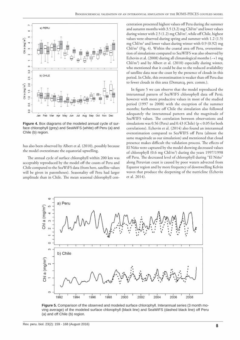
In �gure 5 we can observe that the model reproduced the interannual pattern of SeaWIFS chlorophyll data o� Perú; however with more productive values in most of the studied period (1997 to 2008) with the exception of the summer months; furthermore o� Chile the simulation also followed adequately the interannual pattern and the magnitude of SeaWIFS values. �e correlation between observations and simulations was 0.56 (Peru) and 0.43 (Chile) (p < 0.05 for both correlations). Echevin et al. (2014) also found an interannual overestimation compared to SeaWIFS o� Peru (almost the same magnitude as our simulation) and mentioned that cloud presence makes di�cult the validation process. �e e�ects of El Niño were captured by the model showing decreased values of chlorophyll (0.6 mg Chl/m3) during the years 1997/1998 o� Peru. �e decreased level of chlorophyll during “El Niño” along Peruvian coast is caused by poor waters advected from Equator region and by more frequency of downwelling Kelvin waves that produce the deepening of the nutricline (Echevin et al. 2014).

Figure 5. C omparison of the observed and modeled surface chlorophyll. Interannual series (3 month mo-ving average) of the modeled surface chlorophyll (black line) and SeaW iF S (dashed black line) off Peru (a) and off C hile (b) region.

164



Taylor diagram (Fig. 6) comparing climatological and inte-rannual variations of chlorophyll in the areas o� Peru and Chile within 200 km of the coast showed that the model has a better goodness of �t o� Peru than o� Chile; and in addition, goodness of �t was better for the chlorophyll seasonal cycle than for the interannual variation in both areas.

Surface nutrients.- Nutrients climatology from CARS was also interpolated on 18 km resolution grid and simulated nu-

trients climatology was calculated for the period 1992 – 2008 to be comparable with CARS data, taking into account about 50 years of observed data.

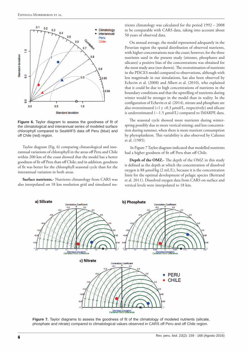
On annual average, the model represented adequately in the Peruvian region the spatial distribution of observed nutrients, with higher concentrations near the coast; however, for the three nutrients used in the present study (nitrates, phosphates and silicates) a positive bias of the concentrations was obtained for the most study area (not shown). �e overestimation of nutrients in the PISCES model compared to observations, although with less magnitude in our simulations, has also been observed by Echevin et al. (2008) and Albert et al. (2010), who explained that it could be due to high concentrations of nutrients in the boundary conditions and that the upwelling of nutrients during winter would be stronger in the model than in reality. In the con�guration of Echevin et al. (2014), nitrate and phosphate are also overestimated (+1 y +0.3 µmol/L, respectively) and silicate is underestimated (~-1.5 µmol/L) compared to IMARPE data.

�e seasonal cycle showed more nutrients during winter-spring possibly due to more vertical mixing; and less concentra-tion during summer, when there is more nutrient consumption by phytoplankton. �is variability is also observed by Calienes et al. (1985).

In Figure 7 Taylor diagram indicated that modelled nutrients had a higher goodness of �t o� Peru than o� Chile.

Depth of the OMZ.- �e depth of the OMZ in this study is de�ned as the depth at which the concentration of dissolved oxygen is 88 µmol/kg (2 mL/L), because it is the concentration limit for the optimal development of pelagic species (Bertrand et al. 2011). Dissolved oxygen data from CARS on surface and vertical levels were interpolated to 18 km.

Figure 6. Taylor diagram to assess the goodness of fit of the climatological and interannual series of modeled surface chlorophyll compared to SeaW IF S data off Peru (blue) and off C hile (red) region.

Figure 7. Taylor diagrams to assess the goodness of fit of the climatology of modeled nutrients (silicate, phosphate and nitrate) compared to climatological values observed in C ARS off Peru and off C hile region.

165



Figure 8. Annual average OMZ depth in meters, defined by the 88 µ mol O2/ k g isoline from ROMS-PISC E S model (a) and C ARS data (b). Map of the RMSE values (c) and the bias (d) calculated of the OMZ depth from PISC E S model and C ARS data for the period simulation.

�e model represented adequately the spatial distribution of the depth of the OMZ, with a shallower OMZ near the ocean o� Peru, as observed in CARS (Fig. 8a and 8b). �e presence of a stronger and shallower OMZ o� Peru could be due to: 1) a high rate of remineralization in�uenced by high primary productivity, 2) a lack of ventilation due to the presence of a strong pycnocline that keeps subsurface waters isolated from the atmosphere, plus deoxygenation of equatorial currents that are the main source of oxygen in this zone (Stramma et al 2010.) and; 3) the long residence time of the waters with a cumulative reduction of oxygen (Czeschel et al. 2011).

RMSE values �uctuated between 0 to 50 µmol/kg and the bias between -20 to 40 µmol/kg. Lower values of RMSE and bias were obtained o� Peru; however, an underestimation in the equatorial zone and an overestimation at the south of the HCLME (between 20ºS to 40ºS) of the depth of the OMZ was observed (Fig. 8c and 8d). �e greatest di�erences observed at the equator and at the south of the HCLME could be due to a slight lack of representativeness of the intensities of the cu-rrents in the boundary conditions used in the con�guration of our simulation in these areas, which could lead to less oxygen �ow in the equatorial zone and greater oxygen �ow o� Peru (Espinoza-Morriberón 2012).

�e model represented adequately the seasonal signal of the OMZ upper limit depth o� Peru; however the values from CARS and IMARPE were underestimated on average throughout the year. �e OMZ is shallower during the summer-autumn and deeper during winter-spring (Fig. 9b), probably related to: (a) during winter the vertical mixing is stronger due to more

wind intensity and (b) during autumn after high phytoplank-ton biomass dying, organic matter is consumed by bacteria during the remineralization process with a consequently high consumption of dissolved oxygen (Libes 1992, Paulmier et al. 2006). Interannually, the model reproduced the oxygenation events during "El Niño" (shallower OMZ) and the observed dissolved oxygen from IMARPE; however, it presented some de�ciencies in following the interannual pattern (Fig. 9a). �e correlation between simulations and observations o� Peru was 0.42 (p<0.05). �e deepening of the OMZ during “El Niño” could be due to the impact of Kelvin waves and the intrusion of surface tropical waters rich in oxygen and poor in nutrients. Taylor diagram (Fig. 9c) showed for OMZ depth that correla-tion with IMARPE data was higher for the climatology than for interannual variations.

In other hand, vertically the model reproduced relatively well the vertical structure of dissolved oxygen o� Peru and Chile compared to CARS data (Fig. 10); however, the modeled OMZ o� Peru tend to be larger than CARS OMZ. �e grea-ter intensity of the OMZ in front of Peru is the result of high primary production reproduced in the model; another aspect to consider is the values of the remineralization of dissolved organic carbon (0.3 d−1) and nitri�cation (0.05 d−1) rates used in our con�guration that in�uence oxygen consumption in the model (Espinoza-Morriberón 2012). Sensitivity studies of PISCES model at di�erent values of these parameters need to be explored in the future. CARS climatological data base could also present de�ciencies in accurately represent the values within the OMZ, because they are based on World Ocean Atlas (WOA)

166



Figure 9. OMZ depth in meters, defined by the 88 µmol O2/ k g isoline. (a) Mean monthly series (3 month moving average) from 1992 to 2008 of the modeled OMZ depth (black line) and observed data from IMARPE (dashed blue line) off Peru; (b) seasonal variation of modeled OMZ depth (black line), the observed OMZ depth in C ARS (dashed black line) and IMARPE data (dashed blue line) off Peru; and (c) T aylor diagram assessing the goodness of fit of the climato-logical and interannual series of modeled OMZ depth compared to observed OMZ depth from C ARS and IMARPE respectively off Peru. T he time series w ere computed w ithin 0-200 km from the coast and from 4 ° S to 16° S.

Figure 10. Z onal section at 10º S (top) and 30º S (bottom) of the annual average of modeled dissolved oxygen (left) and ob-served data in C ARS (right) in µ mol/ kg from 0 to 1000 meters in depth.

167



data, which tend to overestimate the O2 within the OMZ due to various factors such as: positive biases in old measurements, interpolation artifacts and the e�ects of variability in ocean circulation (Bianchi et al. 2012).

Coupled ROMS-PISCES model has been validated in other works for the Peruvian region, explaining the interactions of phytoplankton and nutrients in climatological (Echevin et al. 2008, Albert et al. 2010) and interannual (Echevin et al. 2014) mode; however in the present con�guration we repro-duced the interannual dynamics of biogeochemical variables on a longer period (17 years) and during the occurrence of an extreme El Niño (1997−1998). On the other hand, the dissolved oxygen dynamics was studied and we could observe El Nino impact on it.

Conclusions�e present con�guration of the ROMS-PISCES model re-

produced adequately the dynamics of the main biogeochemical variables (chlorophyll, nutrients and the depth of the oxycline) in the HCLME. �e model showed a very productive system near the coast and the seasonal cycles of chlorophyll, nutrients and depth of the OMZ were acceptably reproduced. Regarding the interannual signal, the model captured well the decrease in chlorophyll concen-tration and the increase in OMZ depth produced by "El Niño"; however we have to keep in mind that the model represented the climatological variations better than the interannual variations.

It is noteworthy that this study presents one of the �rst at-tempts to reproduce the dynamics of biogeochemical variables in the HCLME (Echevin et al. 2008, Albert et al. 2010, Echevin et al. 2014, Montes et al. 2014). However, the present con�-guration of the model still has several problems to be solved. It is necessary to conduct sensitivity analysis of the model with di�erent boundary conditions, forcings and di�erent values of key parameters of the PISCES model, such as rates of remine-ralization and nitri�cation, among others.

AcknowledgementsWe acknowledge Christophe Hourdin for providing model

con�gurations and running the simulation performed within the PEPS project, Carlos Quispe from LMOECC (IMARPE) for their valuable comments on the statistical analysis. �is work was published with the support of IRD and the JEAI EMACEP (Ecología Marina Cuantitativa del Ecosistema de A�oramiento Peruano) and the LMI DISCOH (Dinamica de Sistema de Corriente de Humboldt).

Literature citedAlbert A., V. Echevin, M. Levy, et al. 2010. Impact of the near-

shore wind stress curl on coastal circulation and pri-mary productivity in the Peru upwelling system. Journal of Geophysical Research 115:C12033. doi: http://dx.doi.org/10.1029/2010JC006569.

Aumont O. & L. Bopp. 2006. Globalizing results from ocean in situ iron fertilization studies. Global Biogeochemical Cycles 20:GB2017. doi: http://dx.doi.org/10.1029/2005GB00259.

Behrenfeld M. & P. Falkowski. 1997. Photosynthetic rates derived from satellite-based chlorophyll concentration. Limnology and Oceanography 42(1):1-20. doi: http://dx.doi.org/10.4319/lo.1997.42.1.0001.

Bertrand A., A. Chaigneau, S. Peraltilla, et al. 2011. Oxygen: A fundamental property regulating pelagic ecosystem struc-ture in the coastal southeastern Tropical Paci�c. PLoS One 6(12):e29558. doi: http://dx.doi.org/10.1371/annotation/891b6bd0-185f-4f5f-9f0c-d2408a31f7f4.

Bianchi D., J.P. Dunne, J.L. Sarmiento, et al. 2012. Data-based estimates of suboxia, denitri�cation, and N2O production in the ocean and their sensitivities to dissolved O2. Global Biogeochemical Cycles 26:GB2009. doi: http://dx.doi.org/10.1029/2011GB004209.

Bruland, K., E. Rue, G. Smith, et al. 2005. Iron, macronutrients and diatom blooms in the Perú upwelling regime: brown and blue waters of Peru. Marine Chemestry 93: 81-103. doi: http://dx.doi.org/10.1016/j.marchem.2004.06.011.

Calienes R., O. Guillén & N. Lostaunau. 1985. Variabilidad espacio-temporal de cloro�la, producción primaria y nutrientes frente a la costa peruana. Boletin del Instituto del Mar del Perú - Callao 10:1-44.

Cambon G., K. Goubanova, P. Marchesiello, et al. 2013. Assessing the impact of downscaled atmospheric winds on a regional ocean model simulation of the Humboldt system. Ocean Modelling 65:11-24. doi: http://dx.doi.org/10.1016/j.ocemod.2013.01.007.

Colas F., X. Capet, J. C. McWilliams, et al. 2008. 1997–1998 El Nino o� Peru: A numerical study. Progress in Ocean-ography 79:138–155. doi: http://dx.doi.org/10.1016/j.pocean.2008.10.015.

Czeschel R., L. Stramma, F.U. Schwarzkopf, et al. 2011. Mid depth circulation of the eastern tropical South Pacific and its link to the oxygen minimum zone. Journal of Geophysical Research 116: C01015. doi: http://dx.doi.org/10.1029/2010JC006565.

Da Silva A.M., C.C. Young & s. Levitus. 1994. Atlas of surface marina data 1994. Technical report, Natl. Oceanogr. And Atmos. Admin. Silver Spring Md.

Echevin V., O. Aumont, J. Ledesma, et al. 2008. �e seasonal cycle of surface chlorophyll in the Peruvian upwelling system: A model study. Progress in Oceanography 79: 167-176. doi: http://dx.doi.org/10.1016/j.pocean.2008.10.026.

Echevin V., K. Goubanova, B. Dewitte, et al. 2012. Sensitivity of the Humboldt Current system to global warming: a downscaling experiment of the IPSL-CM4 model. Climate Dynamics 38(3-4):761-774. doi: http://dx.doi.org/10.1007/s00382-011-1085-2.

Echevin V., A. Albert, M. Lévy, et al. 2014. Intraseasonal variability of nearshore productivity in the Northern Humboldt Current System: �e Role of coastal trapped waves. Continental Shelf Research 73: 14-30. doi: http://dx.doi.org/10.1016/j.csr.2013.11.015.

Echevin, V. 2010. Peru Ecosystem Projection Scenarios. ANR. On line: https://skyros.locean-ipsl.upmc.fr/~peps/

Edwards A.M. 2001. Adding detritus to a nutrient–phytoplankton-zooplankton model: a dynamical-systems approach. Journal of Plankton Research 23(4): 389-413. doi: http://dx.doi.org/10.1093/plankt/23.4.389.

Espinoza-Morriberón D. 2012. Impacto de la circulación ecuatorial en la zona mínima de oxígeno presente en el norte del Eco-sistema de la Corriente de Humboldt. �esis to obtain the degree of Master in Marine Sciences. Unidad de Postgrado Víctor Alzamora. Facultad de Ciencia y Filosofía. Universi-dad Peruana Cayetano Heredia, Lima. 115 pp.

Lehmann M.K., K. Fennel & R. He 2009. Statistical validation of a 3-D bio-physical model of the western North Atlantic. Bio-geosciences 6: 1961–1974. doi: http://dx.doi.org/10.5194/bg-6-1961-2009.

Garcia H.E., R.A. Locarnini, T.P. Boyer, et al. 2010. World Ocean Atlas 2009, Volume 3: Dissolved Oxygen, Apparent Oxygen Utilization, and Oxygen Saturation. S. Levitus, Ed. NOAA Atlas NESDIS 70, U.S. Government Printing O�ce, Wash-ington, D.C., 344 pp.

Gruber N., H. Frenzel, S.C. Doney, et al. 2006. Eddy-resolving simu-lation of plankton ecosystem dynamics in the California Current System. Deep Sea Research 1(53): 1483-1516. doi: http://dx.doi.org/10.1016/j.dsr.2006.06.005.

Gutknecht E., I. Dadou, B. Le Vu, et al. 2013. Coupled physical/bio-geochemical modeling including O2-dependent processes in Eastern Boundary Upwelling Systems: Application in the Benguela. Biogeosciences 10: 3559–3591. doi: http://dx.doi.org/10.5194/bg-10-3559-2013.

168



Heinle A. & Slawig T. 2013. Internal Dynamics of NPZD type ecosys-tem models. Ecological Modelling 254: 33 – 42. doi: http://dx.doi.org/10.1016/j.ecolmodel.2013.01.012.

Illig S., B. Dewitte, K. Goubanova, et al. 2014. Forcing mechanisms of intraseasonal SST variability o� central Peru in 2000-2008. Journal of Geophysical Research Oceans 119(6):3548-3573. doi: http://dx.doi.org/10.1002/2013JC009779

Libes S. 1992. Introduction to Marine Biogeochemistry. John Wiley & Sons. Inc. Nueva York. 734 pp.

Montes I., F. Colas, X. Capet, et al. 2010. On the pathways of the equatorial subsurface currents in the eastern equatorial Pa-ci�c and their contributions to the Peru Chile Undercurrent. Journal of Geophysical Research 115: C09003. doi: http://dx.doi.org/10.1029/2009JC005710.

Montes I., B. Dewitte, E. Gutknecht, et al. 2014. High-resolution modeling of the Eastern Tropical Paci�c oxygen minimum zone: Sensitivity to the tropical oceanic circulation, Journal of Geophysical Research Oceans. 119. doi: http://dx.doi.org/10.1002/2014JC009858.

Musial J.P., M.M. Verstraete & N. Gobron. 2011. Comparing the e�ectiveness of recent algorithms to �ll and smooth incom-plete and noisy time series. Atmospheric Chemistry and Physics 11: 14259–14308. doi: http://dx.doi.org/10.5194/acpd-11-14259-2011

Nixon S & A. �omas. 2001. On the size of the Peru upwelling eco-system. Deep Sea Research I 48: 2521–2528. doi: http://dx.doi.org/10.1016/S0967-0637(01)00023-1.

Paulmier A, D. Ruiz-Pino, V. Garçon, et al. 2006. Maintaining of the Eastern South Paci�c Oxygen Minimum Zone (OMZ) o� Chile. Geophysical Research Letter 33: L20601. doi: http://dx.doi.org/10.1029/2006GL026801.

Penven P., V. Echevin, J. Pasapera, et al. 2005. Average circula-tion, seasonal cycle, and mesoscale dynamics of the Peru Current System: A modeling approach. Journal of Geophysical Research 110: C10021. doi: http://dx.doi.org/10.1029/2005JC002945.

Red�eld A.C., B.H. Ketchum & F.A. Richards. 1963. �e in�uence of organisms on the composition of the sea-water. En: Hill M.N. (Eds.). Interscience 2: 26-77.

Ridgway K.R., J.R. Dunn & J.L. Wilkin. 2002. Ocean interpola-tion by four-dimensional least squares-Application to the waters around Australia. Journal of Atmospheric and Oceanic Technology 19(9):1357-1375. doi: http://dx.doi.org/10.1175/1520-0426(2002)019<1357:OIBFDW>2.0.CO;2.

Risien C.M. & D.B. Chelton. 2008. A Global Climatology of Surface Wind and Wind Stress Fields from Eight Years of QuikSCAT Scatterometer Data. Journal of Physi-cal Oceanography 38: 2379-2413. doi: http://dx.doi.org/10.1175/2008JPO3881.1.

Shchepetkin A.F. & J.C. McWilliams. 2005. �e regional oceanic mod-eling system: a split-explicit, free-surface, topography-follow-ing-coordinate ocean model. Ocean Modelling 9: 347–404. doi: http://dx.doi.org/10.1016/j.ocemod.2004.08.002.

Stramma L., G. Johnson, E. Firing, et al. 2010. Eastern Paci�c oxygen minimum zones: Supply paths and multidecadal changes. Journal of Geophysical Research 115:C09011. doi: http://dx.doi.org/10.1029/2009JC005976.

Taylor K.E. 2001. Summarizing multiple aspects of model performance in a single diagram. Journal of Geophysical Research 106: 7183–7192. doi: http://dx.doi.org/10.1029/2000JD900719

Traver M. & Y.J. Shin. 2010. Spatio-temporal variability in �sh-induced predation mortality on plankton: A simulation approach using a coupled trophic model of the Benguela ecosystem. Progress in Oceanography 84(1-2):118-120. doi: http://dx.doi.org/10.1016/j.pocean.2009.09.014

Vichi M. & S. Masina. 2009. Skill assessment of the PELAGOS global ocean biogeochemistry model over the period 1980–2000. Biogeosciences 6: 2333–2353. doi: http://dx.doi.org/10.5194/bg-6-2333-2009.

biogeochemical validation of an interannual simulation of ... · southeast pacific. revista peruana...

Documents