bioinformatics toolbox 2 reference -...
TRANSCRIPT

Bioinformatics Toolbox 2Reference

How to Contact The MathWorks
www.mathworks.com Webcomp.soft-sys.matlab Newsgroupwww.mathworks.com/contact_TS.html Technical Support
[email protected] Product enhancement [email protected] Bug [email protected] Documentation error [email protected] Order status, license renewals, [email protected] Sales, pricing, and general information
508-647-7000 (Phone)
508-647-7001 (Fax)
The MathWorks, Inc.3 Apple Hill DriveNatick, MA 01760-2098For contact information about worldwide offices, see the MathWorks Web site.
Bioinformatics Toolbox Reference
© COPYRIGHT 2003–2007 by The MathWorks, Inc.The software described in this document is furnished under a license agreement. The software may be usedor copied only under the terms of the license agreement. No part of this manual may be photocopied orreproduced in any form without prior written consent from The MathWorks, Inc.
FEDERAL ACQUISITION: This provision applies to all acquisitions of the Program and Documentationby, for, or through the federal government of the United States. By accepting delivery of the Program orDocumentation, the government hereby agrees that this software or documentation qualifies as commercialcomputer software or commercial computer software documentation as such terms are used or definedin FAR 12.212, DFARS Part 227.72, and DFARS 252.227-7014. Accordingly, the terms and conditions ofthis Agreement and only those rights specified in this Agreement, shall pertain to and govern the use,modification, reproduction, release, performance, display, and disclosure of the Program and Documentationby the federal government (or other entity acquiring for or through the federal government) and shallsupersede any conflicting contractual terms or conditions. If this License fails to meet the government’sneeds or is inconsistent in any respect with federal procurement law, the government agrees to return theProgram and Documentation, unused, to The MathWorks, Inc.
Trademarks
MATLAB, Simulink, Stateflow, Handle Graphics, Real-Time Workshop, and xPC TargetBoxare registered trademarks, and SimBiology, SimEvents, and SimHydraulics are trademarks ofThe MathWorks, Inc.
Other product or brand names are trademarks or registered trademarks of their respectiveholders.
Patents
The MathWorks products are protected by one or more U.S. patents. Please seewww.mathworks.com/patents for more information.

Revision HistoryMay 2005 Online only New for Version 2.1 (Release 14SP2+)September 2005 Online only Revised for Version 2.1.1 (Release 14SP3)November 2005 Online only Revised for Version 2.2 (Release 14SP3+)March 2006 Online only Revised for Version 2.2.1 (Release 2006a)May 2006 Online only Revised for Version 2.3 (Release 2006a+)September 2006 Online only Revised for Version 2.4 (Release 2006b)March 2007 Online only Revised for Version 2.5 (Release 2007a)

Contents
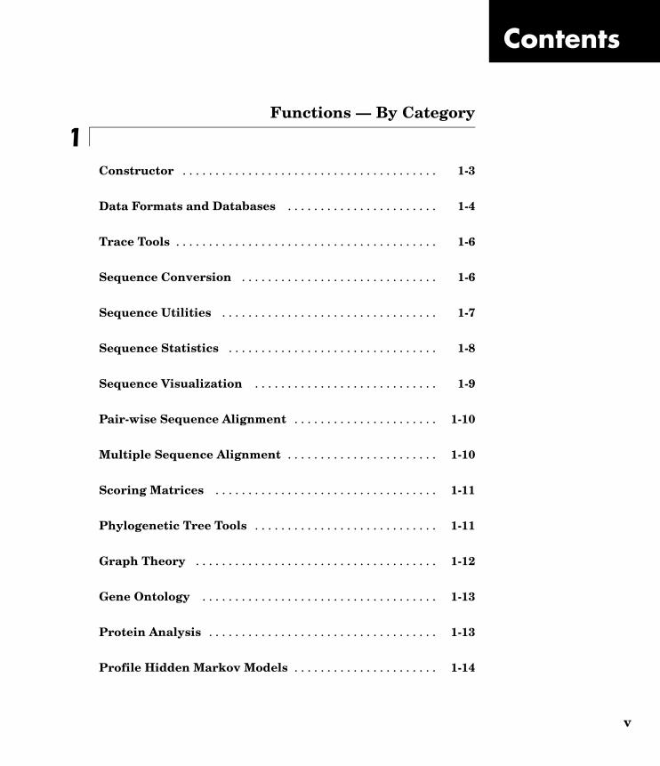
Functions — By Category
1Constructor . . . . . . . . . . . . . . . . . . . . . . . . . . . . . . . . . . . . . . . 1-3
Data Formats and Databases . . . . . . . . . . . . . . . . . . . . . . . 1-4
Trace Tools . . . . . . . . . . . . . . . . . . . . . . . . . . . . . . . . . . . . . . . . 1-6
Sequence Conversion . . . . . . . . . . . . . . . . . . . . . . . . . . . . . . 1-6
Sequence Utilities . . . . . . . . . . . . . . . . . . . . . . . . . . . . . . . . . 1-7
Sequence Statistics . . . . . . . . . . . . . . . . . . . . . . . . . . . . . . . . 1-8
Sequence Visualization . . . . . . . . . . . . . . . . . . . . . . . . . . . . 1-9
Pair-wise Sequence Alignment . . . . . . . . . . . . . . . . . . . . . . 1-10
Multiple Sequence Alignment . . . . . . . . . . . . . . . . . . . . . . . 1-10
Scoring Matrices . . . . . . . . . . . . . . . . . . . . . . . . . . . . . . . . . . 1-11
Phylogenetic Tree Tools . . . . . . . . . . . . . . . . . . . . . . . . . . . . 1-11
Graph Theory . . . . . . . . . . . . . . . . . . . . . . . . . . . . . . . . . . . . . 1-12
Gene Ontology . . . . . . . . . . . . . . . . . . . . . . . . . . . . . . . . . . . . 1-13
Protein Analysis . . . . . . . . . . . . . . . . . . . . . . . . . . . . . . . . . . . 1-13
Profile Hidden Markov Models . . . . . . . . . . . . . . . . . . . . . . 1-14
v
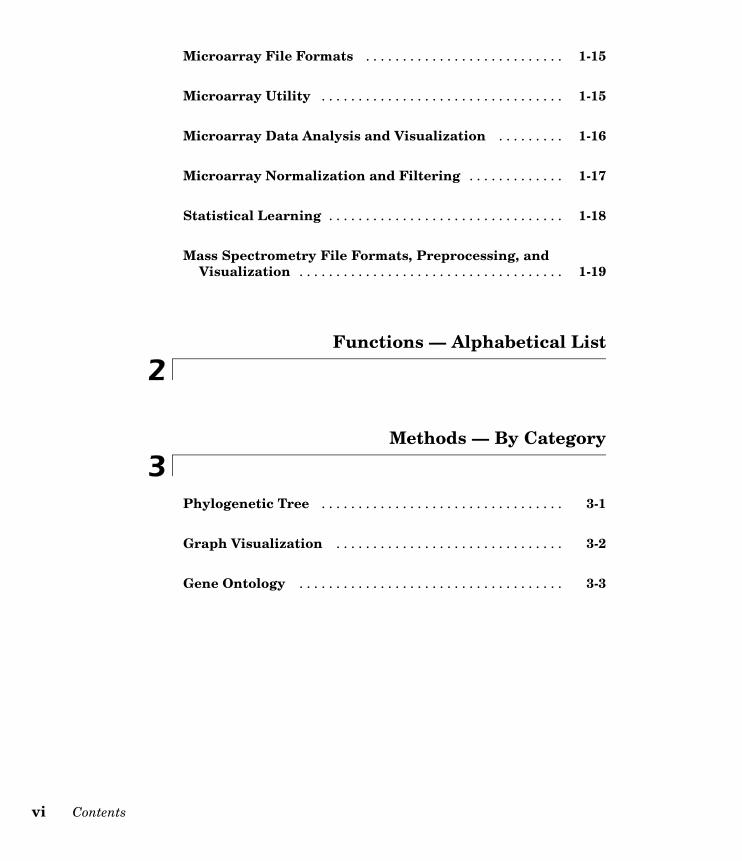
Microarray File Formats . . . . . . . . . . . . . . . . . . . . . . . . . . . 1-15
Microarray Utility . . . . . . . . . . . . . . . . . . . . . . . . . . . . . . . . . 1-15
Microarray Data Analysis and Visualization . . . . . . . . . 1-16
Microarray Normalization and Filtering . . . . . . . . . . . . . 1-17
Statistical Learning . . . . . . . . . . . . . . . . . . . . . . . . . . . . . . . . 1-18
Mass Spectrometry File Formats, Preprocessing, andVisualization . . . . . . . . . . . . . . . . . . . . . . . . . . . . . . . . . . . . 1-19
Functions — Alphabetical List
2
Methods — By Category
3Phylogenetic Tree . . . . . . . . . . . . . . . . . . . . . . . . . . . . . . . . . 3-1
Graph Visualization . . . . . . . . . . . . . . . . . . . . . . . . . . . . . . . 3-2
Gene Ontology . . . . . . . . . . . . . . . . . . . . . . . . . . . . . . . . . . . . 3-3
vi Contents

Methods — Alphabetical List
4
Objects — Alphabetical List
5
Index
vii

viii Contents

1
Functions — By Category
Constructor (p. 1-3) Create objects
Data Formats and Databases (p. 1-4) Get data into MATLAB® from Webdatabases; read and write to filesusing specific sequence data formats
Trace Tools (p. 1-6) Read data from SCF file and drawnucleotide trace plots
Sequence Conversion (p. 1-6) Convert nucleotide and aminoacid sequences between characterand integer formats, reverse andcomplement order of nucleotidebases, and translate nucleotidescodons to amino acids
Sequence Utilities (p. 1-7) Calculate consensus sequence fromset of multiply aligned sequences,run BLAST search from MATLAB,and search sequences using regularexpressions
Sequence Statistics (p. 1-8) Determine base counts, nucleotidedensity, codon bias, and CpG islands;search for words and identify openreading frames (ORFs)
Sequence Visualization (p. 1-9) Visualize sequence data
Pair-wise Sequence Alignment(p. 1-10)
Compare nucleotide or amino acidsequences using pair-wise sequencealignment functions

1 Functions — By Category
Multiple Sequence Alignment(p. 1-10)
Compare sets of nucleotide or aminoacid sequences; progressively alignsequences using phylogenetic treefor guidance
Scoring Matrices (p. 1-11) Standard scoring matrices suchas PAM and BLOSUM families ofmatrices that alignment functionsuse.
Phylogenetic Tree Tools (p. 1-11) Read phylogenetic tree files,calculate pair-wise distancesbetween sequences, and build aphylogenetic tree
Graph Theory (p. 1-12) Apply basic graph theory algorithmsto sparse matrices
Gene Ontology (p. 1-13) Read Gene Ontology formatted files
Protein Analysis (p. 1-13) Determine protein characteristicsand simulate enzyme cleavagereactions
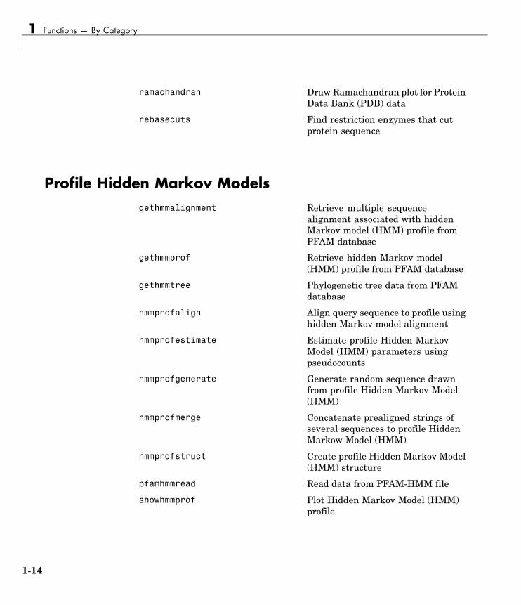
Profile Hidden Markov Models(p. 1-14)
Get profile hidden Markov modeldata from the PFAM database orcreate your own profiles from set ofsequences
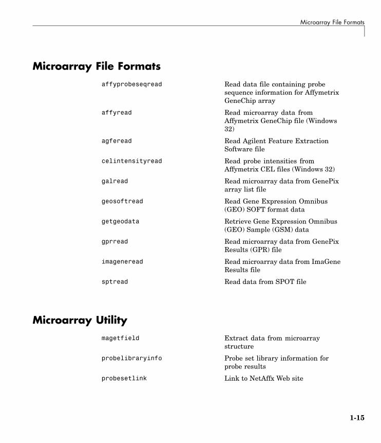
Microarray File Formats (p. 1-15) Read data from common microarrayfile formats including Affymetrix®
GeneChip®, ImaGene results, andSPOT files; read GenePix GPR andGAL files
Microarray Utility (p. 1-15) Using Affymetrix and GeneChipdata sets, get library information forprobe, gene information from probeset, and probe set values from CELand CDF information; show probeset information from NetAffx andplot probe set values
1-2

Constructor
Microarray Data Analysis andVisualization (p. 1-16)
Analyze and visualize microarraydata with t tests, spatial plots, boxplots, loglog plots, and intensity-ratioplots
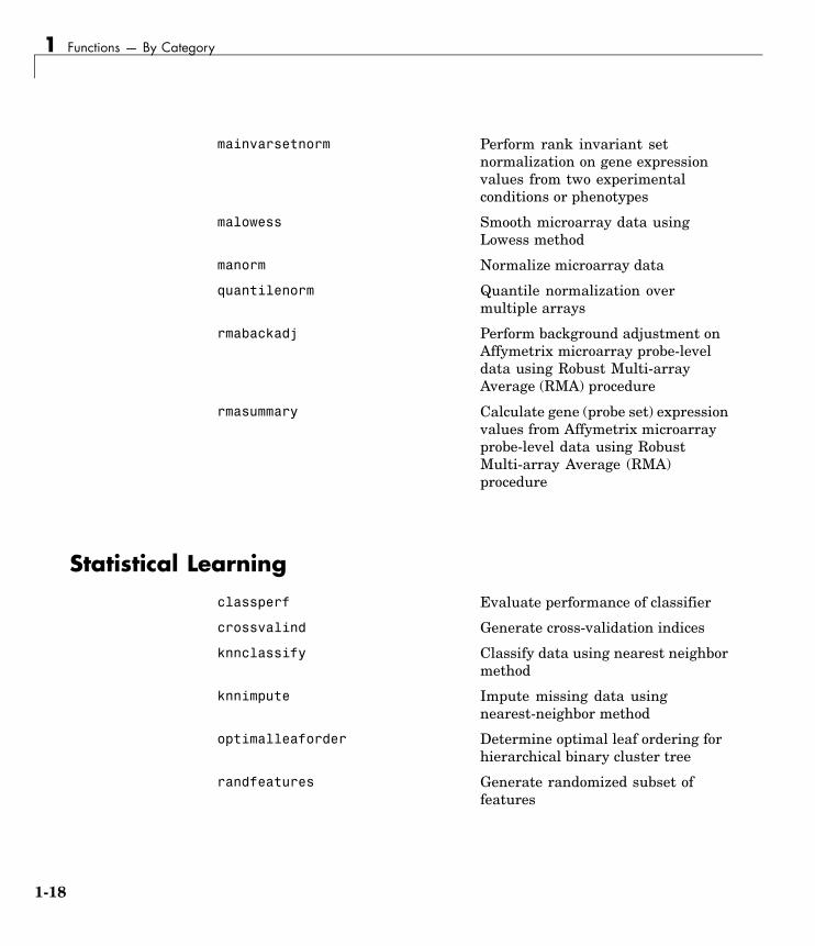
Microarray Normalization andFiltering (p. 1-17)
Normalize microarray data withlowess and mean normalizationfunctions; filter raw data for cleanupbefore analysis
Statistical Learning (p. 1-18) Classify and identify features indata sets, set up cross-validationexperiments, and compare differentclassification methods
Mass Spectrometry File Formats,Preprocessing, and Visualization(p. 1-19)
Read data from common massspectrometry file formats, preprocessraw mass spectrometry data frominstruments, and analyze spectra toidentify patterns and compounds
Constructorbiograph Create biograph object
geneont Create geneont object
phytree Create phytree object
1-3

1 Functions — By Category
Data Formats and Databasesaffyprobeseqread Read data file containing probe
sequence information for AffymetrixGeneChip array
affyread Read microarray data fromAffymetrix GeneChip file (Windows32)
agferead Read Agilent Feature ExtractionSoftware file
blastread Read data from NCBI BLAST reportfile
celintensityread Read probe intensities fromAffymetrix CEL files (Windows 32)
emblread Read data from EMBL file
fastaread Read data from FASTA file
fastawrite Write to file using FASTA format
galread Read microarray data from GenePixarray list file
genbankread Read data from GenBank file
genpeptread Read data from GenPept file
geosoftread Read Gene Expression Omnibus(GEO) SOFT format data
getblast BLAST report from NCBI Web site
getembl Sequence information from EMBLdatabase
getgenbank Sequence information from GenBankdatabase
getgenpept Retrieve sequence information fromGenPept database
getgeodata Retrieve Gene Expression Omnibus(GEO) Sample (GSM) data
1-4
Data Formats and Databases
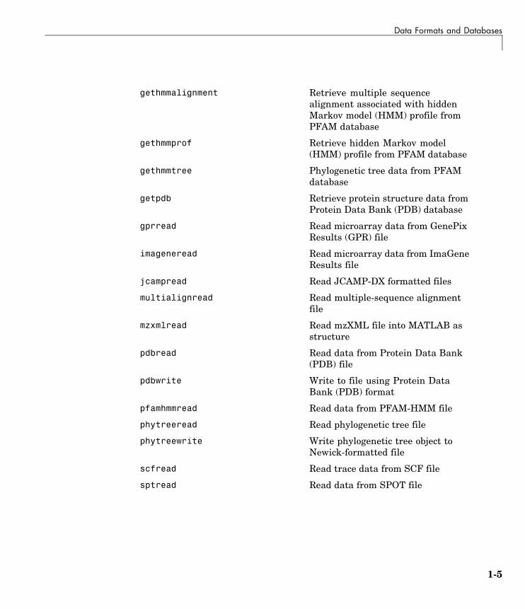
gethmmalignment Retrieve multiple sequencealignment associated with hiddenMarkov model (HMM) profile fromPFAM database
gethmmprof Retrieve hidden Markov model(HMM) profile from PFAM database
gethmmtree Phylogenetic tree data from PFAMdatabase
getpdb Retrieve protein structure data fromProtein Data Bank (PDB) database
gprread Read microarray data from GenePixResults (GPR) file
imageneread Read microarray data from ImaGeneResults file
jcampread Read JCAMP-DX formatted files
multialignread Read multiple-sequence alignmentfile
mzxmlread Read mzXML file into MATLAB asstructure
pdbread Read data from Protein Data Bank(PDB) file
pdbwrite Write to file using Protein DataBank (PDB) format
pfamhmmread Read data from PFAM-HMM file
phytreeread Read phylogenetic tree file
phytreewrite Write phylogenetic tree object toNewick-formatted file
scfread Read trace data from SCF file
sptread Read data from SPOT file
1-5
1 Functions — By Category
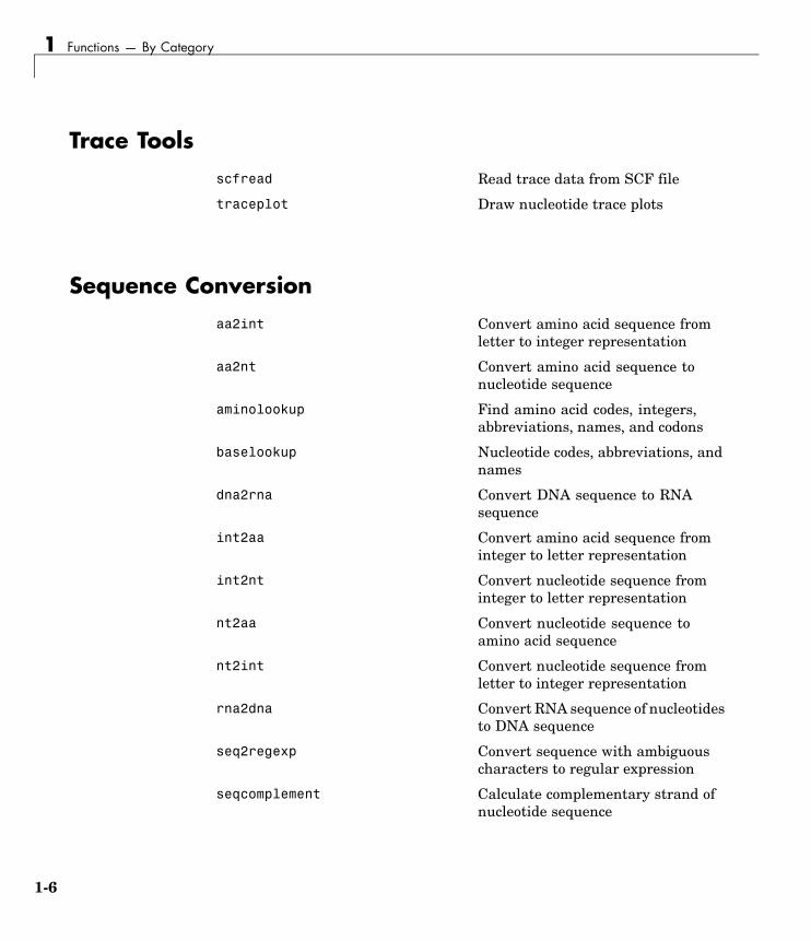
Trace Toolsscfread Read trace data from SCF file
traceplot Draw nucleotide trace plots
Sequence Conversionaa2int Convert amino acid sequence from
letter to integer representation
aa2nt Convert amino acid sequence tonucleotide sequence
aminolookup Find amino acid codes, integers,abbreviations, names, and codons
baselookup Nucleotide codes, abbreviations, andnames
dna2rna Convert DNA sequence to RNAsequence
int2aa Convert amino acid sequence frominteger to letter representation
int2nt Convert nucleotide sequence frominteger to letter representation
nt2aa Convert nucleotide sequence toamino acid sequence
nt2int Convert nucleotide sequence fromletter to integer representation
rna2dna Convert RNA sequence of nucleotidesto DNA sequence
seq2regexp Convert sequence with ambiguouscharacters to regular expression
seqcomplement Calculate complementary strand ofnucleotide sequence
1-6
Sequence Utilities
seqrcomplement Calculate reverse complement ofnucleotide sequence
seqreverse Reverse letters or numbers innucleotide sequence
Sequence Utilitiesaminolookup Find amino acid codes, integers,
abbreviations, names, and codons
baselookup Nucleotide codes, abbreviations, andnames
blastncbi Generate remote BLAST request
cleave Cleave amino acid sequence withenzyme
evalrasmolscript Send RasMol script commands toMolecule Viewer window
featuresparse Parse features from GenBank,GenPept, or EMBL data
geneticcode Nucleotide codon to amino acidmapping
joinseq Join two sequences to produceshortest supersequence
molviewer Display and manipulate 3-Dmolecule structure
oligoprop Calculate sequence properties ofDNA oligonucleotide
palindromes Find palindromes in sequence
pdbdistplot Visualize intermolecular distancesin Protein Data Bank (PDB) file
proteinplot Characteristics for amino acidsequences
1-7

1 Functions — By Category
proteinpropplot Plot properties of amino acidsequence
ramachandran Draw Ramachandran plot for ProteinData Bank (PDB) data
randseq Generate random sequence fromfinite alphabet
rebasecuts Find restriction enzymes that cutprotein sequence
restrict Split nucleotide sequence atrestriction site
revgeneticcode Reverse mapping for genetic code
seqconsensus Calculate consensus sequence
seqdisp Format long sequence output foreasy viewing
seqinsertgaps Insert gaps into nucleotide or aminoacid sequence
seqlogo Display sequence logo for nucleotideor amino acid sequences
seqmatch Find matches for every string inlibrary
seqprofile Calculate sequence profile from setof multiply aligned sequences
seqshoworfs Display open reading frames insequence
Sequence Statisticsaacount Count amino acids in sequence
aminolookup Find amino acid codes, integers,abbreviations, names, and codons
1-8

Sequence Visualization
basecount Count nucleotides in sequence
baselookup Nucleotide codes, abbreviations, andnames
codonbias Calculate codon frequency for eachamino acid in DNA sequence
codoncount Count codons in nucleotide sequence
cpgisland Locate CpG islands in DNA sequence
dimercount Count dimers in sequence
isoelectric Estimate isoelectric point for aminoacid sequence
molweight Calculate molecular weight of aminoacid sequence
nmercount Count number of n-mers innucleotide or amino acid sequence
ntdensity Plot density of nucleotides alongsequence
seqshowwords Graphically display words insequence
seqwordcount Count number of occurrences of wordin sequence
Sequence Visualizationfeaturesmap Draw linear or circular map of
features from GenBank structure
seqtool Open tool to interactively explorebiological sequences
1-9
1 Functions — By Category
Pair-wise Sequence Alignmentfastaread Read data from FASTA file
nwalign Globally align two sequences usingNeedleman-Wunsch algorithm
seqdotplot Create dot plot of two sequences
showalignment Sequence alignment with color
swalign Locally align two sequences usingSmith-Waterman algorithm
Multiple Sequence Alignmentfastaread Read data from FASTA file
multialign Align multiple sequences usingprogressive method
multialignread Read multiple-sequence alignmentfile
multialignviewer Open viewer for multiple sequencealignments
profalign Align two profiles usingNeedleman-Wunsch globalalignment
seqpdist Calculate pair-wise distance betweensequences
showalignment Sequence alignment with color
1-10
Scoring Matrices
Scoring Matricesblosum BLOSUM scoring matrix
dayhoff Dayhoff scoring matrix
gonnet Gonnet scoring matrix
nuc44 NUC44 scoring matrix for nucleotidesequences
pam PAM scoring matrix
Phylogenetic Tree Toolsdnds Estimate synonymous and
nonsynonymous substitutionrates
dndsml Estimate synonymous andnonsynonymous substitutionrates using maximum likelihoodmethod
gethmmtree Phylogenetic tree data from PFAMdatabase
phytreeread Read phylogenetic tree file
phytreetool View, edit, and explore phylogenetictree data
phytreewrite Write phylogenetic tree object toNewick-formatted file
seqinsertgaps Insert gaps into nucleotide or aminoacid sequence
seqlinkage Construct phylogenetic tree frompair-wise distances
1-11
1 Functions — By Category
seqneighjoin Neighbor-joining method forphylogenetic tree reconstruction
seqpdist Calculate pair-wise distance betweensequences
Graph Theorygraphallshortestpaths Find all shortest paths in graph
graphconncomp Find strongly or weakly connectedcomponents in graph
graphisdag Test for cycles in directed graph
graphisomorphism Find isomorphism between twographs
graphisspantree Determine if tree is spanning tree
graphmaxflow Calculate maximum flow andminimum cut in directed graph
graphminspantree Find minimal spanning tree in graph
graphpred2path Convert predecessor indices to paths
graphshortestpath Solve shortest path problem in graph
graphtopoorder Perform topological sort of directedacyclic graph
graphtraverse Traverse graph by following adjacentnodes
1-12

Gene Ontology
Gene Ontologygoannotread Annotations from Gene Ontology
annotated file
num2goid Convert numbers to Gene OntologyIDs
Protein Analysisaacount Count amino acids in sequence
aminolookup Find amino acid codes, integers,abbreviations, names, and codons
atomiccomp Calculate atomic composition ofprotein
cleave Cleave amino acid sequence withenzyme
evalrasmolscript Send RasMol script commands toMolecule Viewer window
isoelectric Estimate isoelectric point for aminoacid sequence
molviewer Display and manipulate 3-Dmolecule structure
molweight Calculate molecular weight of aminoacid sequence
pdbdistplot Visualize intermolecular distancesin Protein Data Bank (PDB) file
proteinplot Characteristics for amino acidsequences
proteinpropplot Plot properties of amino acidsequence
1-13
1 Functions — By Category
ramachandran Draw Ramachandran plot for ProteinData Bank (PDB) data
rebasecuts Find restriction enzymes that cutprotein sequence
Profile Hidden Markov Modelsgethmmalignment Retrieve multiple sequence
alignment associated with hiddenMarkov model (HMM) profile fromPFAM database
gethmmprof Retrieve hidden Markov model(HMM) profile from PFAM database
gethmmtree Phylogenetic tree data from PFAMdatabase
hmmprofalign Align query sequence to profile usinghidden Markov model alignment
hmmprofestimate Estimate profile Hidden MarkovModel (HMM) parameters usingpseudocounts
hmmprofgenerate Generate random sequence drawnfrom profile Hidden Markov Model(HMM)
hmmprofmerge Concatenate prealigned strings ofseveral sequences to profile HiddenMarkow Model (HMM)
hmmprofstruct Create profile Hidden Markov Model(HMM) structure
pfamhmmread Read data from PFAM-HMM file
showhmmprof Plot Hidden Markov Model (HMM)profile
1-14
Microarray File Formats
Microarray File Formatsaffyprobeseqread Read data file containing probe
sequence information for AffymetrixGeneChip array
affyread Read microarray data fromAffymetrix GeneChip file (Windows32)
agferead Read Agilent Feature ExtractionSoftware file
celintensityread Read probe intensities fromAffymetrix CEL files (Windows 32)
galread Read microarray data from GenePixarray list file
geosoftread Read Gene Expression Omnibus(GEO) SOFT format data
getgeodata Retrieve Gene Expression Omnibus(GEO) Sample (GSM) data
gprread Read microarray data from GenePixResults (GPR) file
imageneread Read microarray data from ImaGeneResults file
sptread Read data from SPOT file
Microarray Utilitymagetfield Extract data from microarray
structure
probelibraryinfo Probe set library information forprobe results
probesetlink Link to NetAffx Web site
1-15

1 Functions — By Category
probesetlookup Gene name for probe set
probesetplot Plot values for Affymetrix CHP fileprobe set
probesetvalues Probe set values from probe results
Microarray Data Analysis and Visualizationclustergram Create dendrogram and heat map
maboxplot Box plot for microarray data
mafdr Estimate false discovery rate (FDR)of differentially expressed genesfrom two experimental conditions orphenotypes
maimage Spatial image for microarray data
mairplot Create intensity versus ratio scatterplot of microarray data
maloglog Create loglog plot of microarray data
mapcaplot Create Principal ComponentAnalysis plot of microarray data
mattest Perform two-tailed t-test to evaluatedifferential expression of genesfrom two experimental conditions orphenotypes
mavolcanoplot Create significance versus geneexpression ratio (fold change) scatterplot of microarray data
redgreencmap Create red and green color map
1-16

Microarray Normalization and Filtering
Microarray Normalization and Filteringaffyinvarsetnorm Perform rank invariant set
normalization on probe intensitiesfrom multiple Affymetrix CEL orDAT files
affyprobeaffinities Compute Affymetrix probe affinitiesfrom their sequences and MM probeintensities
exprprofrange Calculate range of gene expressionprofiles
exprprofvar Calculate variance of geneexpression profiles
gcrma Perform GC Robust Multi-arrayAverage (GCRMA) backgroundadjustment, quantile normalization,and median-polish summarizationon Affymetrix microarray probe-leveldata
gcrmabackadj Perform GC Robust Multi-arrayAverage (GCRMA) backgroundadjustment on Affymetrixmicroarray probe-level datausing sequence information
geneentropyfilter Remove genes with low entropyexpression values
genelowvalfilter Remove gene profiles with lowabsolute values
generangefilter Remove gene profiles with smallprofile ranges
genevarfilter Filter genes with small profilevariance
1-17
1 Functions — By Category
mainvarsetnorm Perform rank invariant setnormalization on gene expressionvalues from two experimentalconditions or phenotypes
malowess Smooth microarray data usingLowess method
manorm Normalize microarray data
quantilenorm Quantile normalization overmultiple arrays
rmabackadj Perform background adjustment onAffymetrix microarray probe-leveldata using Robust Multi-arrayAverage (RMA) procedure
rmasummary Calculate gene (probe set) expressionvalues from Affymetrix microarrayprobe-level data using RobustMulti-array Average (RMA)procedure
Statistical Learningclassperf Evaluate performance of classifier
crossvalind Generate cross-validation indices
knnclassify Classify data using nearest neighbormethod
knnimpute Impute missing data usingnearest-neighbor method
optimalleaforder Determine optimal leaf ordering forhierarchical binary cluster tree
randfeatures Generate randomized subset offeatures
1-18

Mass Spectrometry File Formats, Preprocessing, and Visualization
rankfeatures Rank key features by classseparability criteria
svmclassify Classify data using support vectormachine
svmsmoset Create or edit Sequential MinimalOptimization (SMO) optionsstructure
svmtrain Train support vector machineclassifier
Mass Spectrometry File Formats, Preprocessing, andVisualization
jcampread Read JCAMP-DX formatted files
msalign Align peaks in mass spectrum toreference peaks
msbackadj Correct baseline of mass spectrum
msdotplot Plot set of peak lists from LC/MS orGC/MS data set
msheatmap Create pseudocolor image of set ofmass spectra
mslowess Smooth mass spectrum usingnonparametric method
msnorm Normalize set of mass spectra
mspalign Align mass spectra from multiplepeak lists from LC/MS or GC/MSdata set
mspeaks Convert raw mass spectrometry datato peak list (centroided data)
msppresample Resample mass spectrometry signalwhile preserving peaks
1-19

1 Functions — By Category
msresample Resample mass spectrometry signal
mssgolay Smooth mass spectrum withleast-squares polynomial
msviewer Explore mass spectrum or set ofmass spectra
mzxml2peaks Convert mzXML structure to peaklist
mzxmlread Read mzXML file into MATLAB asstructure
1-20
2
Functions — AlphabeticalList

aa2int
Purpose Convert amino acid sequence from letter to integer representation
Syntax SeqInt = aa2int(SeqChar)
Arguments SeqChar Either of the following:• Character string of single-letter codes specifying an
amino acid sequence. See the table Mapping AminoAcid Letters to Integers on page 2-2 for valid codes.Unknown characters are mapped to 0. Integers arearbitrarily assigned to IUB/IUPAC letters.
• Structure containing a Sequence field that contains anamino acid sequence, such as returned by fastaread,getembl, getgenpept, or getpdb.
ReturnValues
SeqInt Row vector of integers specifying an amino acid sequence.
Mapping Amino Acid Letters to Integers
Amino Acid Code Integer
Alanine A 1
Arginine R 2
Asparagine N 3
Aspartic acid (Aspartate) D 4
Cysteine C 5
Glutamine Q 6
Glutamic acid (Glutamate) E 7
Glycine G 8
Histidine H 9
2-2

aa2int
Amino Acid Code Integer
Isoleucine I 10
Leucine L 11
Lysine K 12
Methionine M 13
Phenylalanine F 14
Proline P 15
Serine S 16
Threonine T 17
Tryptophan W 18
Tyrosine Y 19
Valine V 20
Aspartic acid or Asparagine B 21
Glutamic acid or glutamine Z 22
Any amino acid X 23
Translation stop * 24
Gap of indeterminate length - 25
Unknown or any character orsymbol not in table
? 0
Description SeqInt = aa2int(SeqChar) converts SeqChar, a string of single-lettercodes specifying an amino acid sequence, to SeqInt, a 1-by-N arrayof integers specifying the same amino acid sequence. See the tableMapping Amino Acid Letters to Integers on page 2-2 for valid codes.
Examples Converting a Simple Sequence
Convert the sequence of letters MATLAB to integers.
2-3

aa2int
SeqInt = aa2int('MATLAB')
SeqInt =
13 1 17 11 1 21
Converting a Random Sequence
Convert a random amino acid sequence of letters to integers.
1 Create a random character string to represent an amino acidsequence.
SeqChar = randseq(20, 'alphabet', 'amino')
SeqChar =
dwcztecakfuecvifchds
2 Convert the amino acid sequence from letter to integer representation.
SeqInt = aa2int(SeqChar)
SeqInt =
Columns 1 through 134 18 5 22 17 7 5 1 12 14 0 7 5
Columns 14 through 2020 10 14 5 9 4 16
See Also Bioinformatics Toolbox functions: aminolookup, int2aa, int2nt,nt2int
2-4
aa2nt
Purpose Convert amino acid sequence to nucleotide sequence
Syntax SeqNT = aa2nt(SeqAA)aa2nt(..., 'PropertyName', PropertyValue,...)aa2nt(..., 'GeneticCode', GeneticCodeValue)aa2nt(..., 'Alphabet' AlphabetValue)
Arguments SeqAA Amino acid sequence. Enter a characterstring or a vector of integers from the table.Examples: 'ARN' or [1 2 3]
GeneticCodeValue Property to select a genetic code. Enter a codenumber or code name from the Genetic Code onpage 2-5 table below. If you use a code name,you can truncate the name to the first twocharacters of the name.
AlphabetValue Property to select a nucleotide alphabet. Entereither 'DNA' or 'RNA'. The default value is'DNA', which uses the symbols A, C, T, G. Thevalue 'RNA' uses the symbols A, C, U, G.
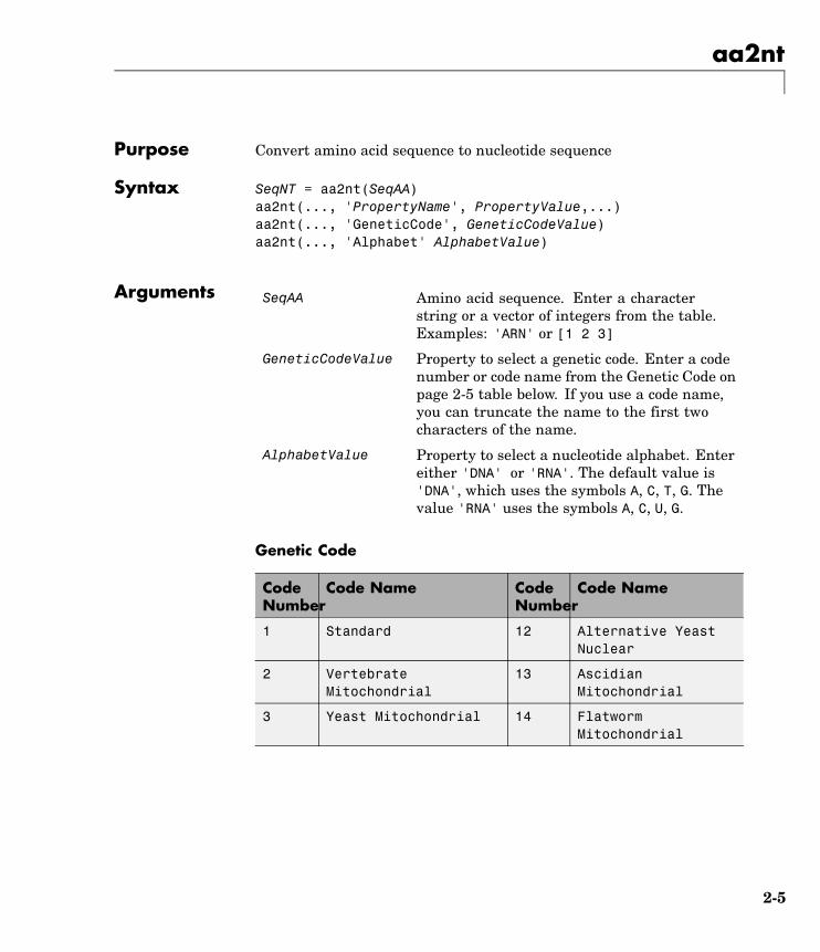
Genetic Code
CodeNumber
Code Name CodeNumber
Code Name
1 Standard 12 Alternative YeastNuclear
2 VertebrateMitochondrial
13 AscidianMitochondrial
3 Yeast Mitochondrial 14 FlatwormMitochondrial
2-5

aa2nt
CodeNumber
Code Name CodeNumber
Code Name
4 Mold, Protozoan,CoelenterateMitochondrial,and Mycoplasma/Spiroplasma
15 Blepharisma Nuclear
5 InvertebrateMitochondrial
16 ChlorophyceanMitochondrial
6 Ciliate, Dasycladacean,and Hexamita Nuclear
21 TrematodeMitochondrial
9 EchinodermMitochondrial
22 Scenedesmus ObliquusMitochondrial
10 Euplotid Nuclear 23 ThraustochytriumMitochondrial
11 Bacterial and PlantPlastid
Description SeqNT = aa2nt(SeqAA) converts an amino acid sequence (SeqAA) toa nucleotide sequence (SeqNT) using the standard genetic code. Ingeneral, the mapping from an amino acid to a nucleotide codon is nota one-to-one mapping. For amino acids with more than one possiblenucleotide codon, this function selects randomly a codon correspondingto that particular amino acid.
For the ambiguous characters B and Z, one of the amino acidscorresponding to the letter is selected randomly, and then a codonsequence is selected randomly. For the ambiguous character X, a codonsequence is selected randomly from all possibilities.
aa2nt(..., 'PropertyName', PropertyValue,...) defines optionalproperties using property name/value pairs.
2-6
aa2nt
aa2nt(..., 'GeneticCode', GeneticCodeValue) selects a geneticcode (GeneticCodeValue) to use when converting an amino acidsequence (SeqAA) to a nucleotide sequence (SeqNT).
aa2nt(..., 'Alphabet' AlphabetValue) selects a nucleotidealphabet (AlphabetValue).
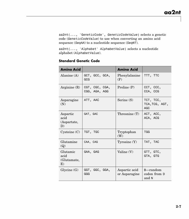
Standard Genetic Code
Amino Acid Amino Acid
Alanine (A) GCT, GCC, GCA,GCG
Phenylalanine(F)
TTT, TTC
Arginine (R) CGT, CGC, CGA,CGG, AGA, AGG
Proline (P) CCT, CCC,CCA, CCG
Asparagine(N)
ATT, AAC Serine (S) TCT, TCC,TCA,TCG, AGT,AGC
Asparticacid(Aspartate,D)
GAT, GAC Threonine (T) ACT, ACC,ACA, ACG
Cysteine (C) TGT, TGC Tryptophan(W)
TGG
Glutamine(Q)
CAA, CAG Tyrosine (Y) TAT, TAC
Glutamicacid(Glutamate,E)
GAA, GAG Valine (V) GTT, GTC,GTA, GTG
Glycine (G) GGT, GGC, GGA,GGG
Aspartic acidor Asparagine
B—randomcodon from Dand N
2-7

aa2nt
Amino Acid Amino Acid
Histidine(H)
CAT, CAC Glutamic acidor Glutamine
Z—randomcodon from Eand Q
Isoleucine(I)
ATT, ATC, ATA Unknown orany amino acid
X randomcodon
Leucine (L) TTA, TTG, CTT,CTC, CTA, CTG
Translationstop (*)
TAA, TAG, TGA
Lysine (K) AAA, AAG Gap ofindeterminatelength (-)
---
Methionine(M)
ATG Any characteror any symbolnot in table (?)
???
Examples 1 Convert an amino acid sequence to a nucleotide sequence using thestandard genetic code.
aa2nt('MATLAB')
Warning: The sequence contains ambiguous characters.ans =ATGGCAACCCTGGCGAAT
2 Use the Vertebrate Mitochondrial genetic code.
aa2nt('MATLAP', 'GeneticCode', 2)
ans =ATGGCAACTCTAGCGCCT
3 Use the genetic code for the Echinoderm Mitochondrial RNAalphabet.
2-8

aa2nt
aa2nt('MATLAB','GeneticCode','ec','Alphabet','RNA')
Warning: The sequence contains ambiguous characters.ans =AUGGCUACAUUGGCUGAU
4 Convert a sequence with the ambiguous amino acid character B.
aa2nt('abcd')
Warning: The sequence contains ambiguous characters.ans =GCCACATGCGAC
See Also Bioinformatics Toolbox functions: geneticcode, nt2aa,revgeneticcode, seqtool
MATLAB function: rand
2-9
aacount
Purpose Count amino acids in sequence
Syntax Amino = aacount(SeqAA)aacount(..., 'PropertyName', PropertyValue,...)aacount(..., 'Chart', ChartValue)aacount(..., 'Others', OthersValue)aacount(..., 'Structure', StructureValue)
ArgumentsSeqAA Amino acid sequence. Enter a character string
or vector of integers from the table. Examples:'ARN' or [1 2 3]. You can also enter a structurewith the field Sequence.
ChartValue Property to select a type of plot. Enter either'pie' or 'bar'.
OthersValue Property to control the counting of ambiguouscharacters individually. Enter either 'full' or'bundle'(default).
StructureValue Property to control blocking the unknowncharacters warning and to not count unknowncharacters.
Description Amino = aacount(SeqAA) counts the type and number of amino acidsin an amino acid sequence (SeqAA) and returns the counts in a 1-by-1structure (Amino) with fields for the standard 20 amino acids (A R N DC Q E G H I L K M F P S T W Y V ).
• If a sequence contains amino acids with ambiguous characters (B, Z,X), the stop character (*), or gaps indicated with a hyphen (-), the fieldOthers is added to the structure and a warning message is displayed.
Warning: Symbols other than the standard 20 amino acidsappear in the sequence.
2-10
aacount
• If a sequence contains any characters other than the 20 standardamino acids, ambiguous characters, stop, and gap characters, thecharacters are counted in the field Others and a warning message isdisplayed.
Warning: Sequence contains unknown characters. These willbe ignored.
• If the property Others = 'full' , this function lists the ambiguouscharacters separately, asterisks are counted in a new field (Stop),and hyphens are counted in a new field (Gap).
aacount(..., 'PropertyName', PropertyValue,...) definesoptional properties using property name/value pairs:
aacount(..., 'Chart', ChartValue) creates a chart showing therelative proportions of the amino acids.
aacount(..., 'Others', OthersValue), when OthersValue is'full'', counts the ambiguous amino acid characters individuallyinstead of adding them together in the field Others.
aacount(..., 'Structure', StructureValue), whenStructureValue is 'full', blocks the unknown characters warningand ignores counting unknown characters.
• aacount(SeqAA) — Display 20 amino acids, and only if there areambiguous and unknown characters, add an Others field with thecounts.
• aacount(SeqAA, 'Others', 'full') — Display 20 amino acids, 3ambiguous amino acids, stops, gaps, and only if there are unknowncharacters, add an Others field with the unknown counts.
• aacount(SeqAA, 'Structure', 'full') — Display 20 aminoacids and always display an Others field. If there are ambiguousand unknown characters, add counts to the Others field; otherwisedisplay 0.
2-11

aacount
• aacount(SeqAA, 'Others', 'full', 'Structure', 'full') —Display 20 amino acids, 3 ambiguous amino acids, stops, gaps, andOthers field. If there are unknown characters, add counts to theOthers field otherwise display 0.
Examples 1 Create a sequence.
Seq = aacount('MATLAB')
2 Count the amino acids in the sequence.
AA = aacount(Seq)
Warning: Symbols other than the standard 20 amino acids appearin the sequence.AA =
A: 2R: 0N: 0D: 0C: 0Q: 0E: 0G: 0H: 0I: 0L: 1K: 0M: 1F: 0P: 0S: 0T: 1W: 0Y: 0V: 0
Others: 1
2-12

aacount
3 Get the count for alanine (A) residues.
AA.Aans =
2
See Also Bioinformatics Toolbox functions aminolookup, atomiccomp, basecount,codoncount, dimercount, isoelectric, molweight, proteinplot,seqtool
2-13
affyinvarsetnorm
Purpose Perform rank invariant set normalization on probe intensities frommultiple Affymetrix CEL or DAT files
Syntax NormData = affyinvarsetnorm(Data)[NormData, MedStructure] = affyinvarsetnorm(Data)... affyinvarsetnorm(..., 'Baseline', BaselineValue, ...)... affyinvarsetnorm(..., 'Thresholds',ThresholdsValue, ...)... affyinvarsetnorm(..., 'StopPrctile',StopPrctileValue, ...)... affyinvarsetnorm(..., 'RayPrctile',RayPrctileValue, ...)... affyinvarsetnorm(..., 'Method', MethodValue, ...)... affyinvarsetnorm(..., 'Showplot', ShowplotValue, ...)
ArgumentsData Matrix of intensity values where each row
corresponds to a perfect match (PM) probeand each column corresponds to an AffymetrixCEL or DAT file. (Each CEL or DAT file isgenerated from a separate chip. All chipsshould be of the same type.)
MedStructure Structure of each column’s intensity medianbefore and after normalization, and the indexof the column chosen as the baseline.
BaselineValue Property to control the selection of the columnindex N from Data to be used as the baselinecolumn. Default is the column index whosemedian intensity is the median of all thecolumns.
2-14

affyinvarsetnorm
ThresholdsValue Property to set the thresholds for the lowestaverage rank and the highest average rank,which are used to determine the invariant set.The rank invariant set is a set of data pointswhose proportional rank difference is smallerthan a given threshold. The threshold foreach data point is determined by interpolatingbetween the threshold for the lowest averagerank and the threshold for the highest averagerank. Select these two thresholds empiricallyto limit the spread of the invariant set, butallow enough data points to determine thenormalization relationship.
ThresholdsValue is a 1-by-2 vector [LT,HT] where LT is the threshold for the lowestaverage rank and HT is threshold for thehighest average rank. Values must be between0 and 1. Default is [0.05, 0.005].
StopPrctileValue Property to stop the iteration process whenthe number of data points in the invariant setreaches N percent of the total number of datapoints. Default is 1.
Note If you do not use this property, theiteration process continues until no more datapoints are eliminated.
RayPrctileValue Property to select the N percentage of thehighest ranked invariant set of data points tofit a straight line through, while the remainingdata points are fitted to a running mediancurve. The final running median curve is apiece-wise linear curve. Default is 1.5.
2-15
affyinvarsetnorm
MethodValue Property to select the smoothing method usedto normalize the data. Enter 'lowess' or'runmedian'. Default is 'lowess'.
ShowplotValue Property to control the plotting of two pairs ofscatter plots (before and after normalization).The first pair plots baseline data versus datafrom a specified column (chip) from the matrixData. The second is a pair of M-A scatter plots,which plots M (ratio between baseline andsample) versus A (the average of the baselineand sample). Enter either 'all' (plot a pair ofscatter plots for each column or chip) or specifya subset of columns (chips) by entering thecolumn number(s) or a range of numbers.
For example:
• ..., 'Showplot', 3, ...) plots datafrom column 3.
• ..., 'Showplot', [3,5,7], ...) plotsdata from columns 3, 5, and 7.
• ... , 'Showplot', 3:9, ...) plotsdata from columns 3 to 9.
Description NormData = affyinvarsetnorm(Data) normalizes the values in eachcolumn (chip) of probe intensities in Data to a baseline reference, usingthe invariant set method. NormData is a matrix of normalized probeintensities from Data.
Specifically, affyinvarsetnorm:
• Selects a baseline index, typically the column whose median intensityis the median of all the columns.
2-16

affyinvarsetnorm
• For each column, determines the proportional rank difference (prd)for each pair of ranks, RankX and RankY, from the sample columnand the baseline reference.
prd = abs(RankX - RankY)
• For each column, determines the invariant set of data points byselecting data points whose proportional rank differences (prd) arebelow threshold, which is a predetermined threshold for a givendata point (defined by the ThresholdsValue property). It repeatsthe process until either no more data points are eliminated, or apredetermined percentage of data points is reached.
The invariant set is data points with a prd < threshold.
• For each column, uses the invariant set of data points to calculatethe lowess or running median smoothing curve, which is used tonormalize the data in that column.
[NormData, MedStructure] = affyinvarsetnorm(Data) also returnsa structure of the index of the column chosen as the baseline and eachcolumn’s intensity median before and after normalization.
Note If Data contains NaN values, then NormData will also containNaN values at the corresponding positions.
... affyinvarsetnorm(..., 'PropertyName',PropertyValue, ...) defines optional properties that use propertyname/value pairs in any order. These property name/value pairs areas follows:
... affyinvarsetnorm(..., 'Baseline', BaselineValue, ...)lets you select the column index N from Data to be the baseline column.Default is the index of the column whose median intensity is the medianof all the columns.
2-17
affyinvarsetnorm
... affyinvarsetnorm(..., 'Thresholds',ThresholdsValue, ...) sets the thresholds for the lowest averagerank and the highest average rank, which are used to determine theinvariant set. The rank invariant set is a set of data points whoseproportional rank difference is smaller than a given threshold. Thethreshold for each data point is determined by interpolating betweenthe threshold for the lowest average rank and the threshold for thehighest average rank. Select these two thresholds empirically tolimit the spread of the invariant set, but allow enough data points todetermine the normalization relationship.
ThresholdsValue is a 1-by-2 vector [LT, HT] where LT is the thresholdfor the lowest average rank and HT is threshold for the highest averagerank. Values must be between 0 and 1. Default is [0.05, 0.005].
... affyinvarsetnorm(..., 'StopPrctile',StopPrctileValue, ...) stops the iteration process when the numberof data points in the invariant set reaches N percent of the total numberof data points. Default is 1.
Note If you do not use this property, the iteration process continuesuntil no more data points are eliminated.
... affyinvarsetnorm(..., 'RayPrctile',RayPrctileValue, ...) selects the N percentage of the highest rankedinvariant set of data points to fit a straight line through, while theremaining data points are fitted to a running median curve. The finalrunning median curve is a piece-wise linear curve. Default is 1.5.
... affyinvarsetnorm(..., 'Method', MethodValue, ...) selectsthe smoothing method for normalizing the data. When MethodValueis 'lowess', affyinvarsetnorm uses the lowess method. WhenMethodValue is 'runmedian', affyinvarsetnorm uses the runningmedian method. Default is 'lowess'.
... affyinvarsetnorm(..., 'Showplot', ShowplotValue, ...)plots two pairs of scatter plots (before and after normalization). The
2-18

affyinvarsetnorm
first pair plots baseline data versus data from a specified column(chip) from the matrix Data. The second is a pair of M-A scatterplots, which plots M (ratio between baseline and sample) versus A(the average of the baseline and sample). When ShowplotValue is'all', affyinvarsetnorm plots a pair of scatter plots for each columnor chip. When ShowplotValue is a number(s) or range of numbers,affyinvarsetnorm plots a pair of scatter plots for the indicated columnnumbers (chips).
For example:
• ..., 'Showplot', 3) plots the data from column 3 of Data.
• ..., 'Showplot', [3,5,7]) plots the data from columns 3, 5,and 7 of Data.
• ..., 'Showplot', 3:9) plots the data from columns 3 to 9 of Data.
2-19
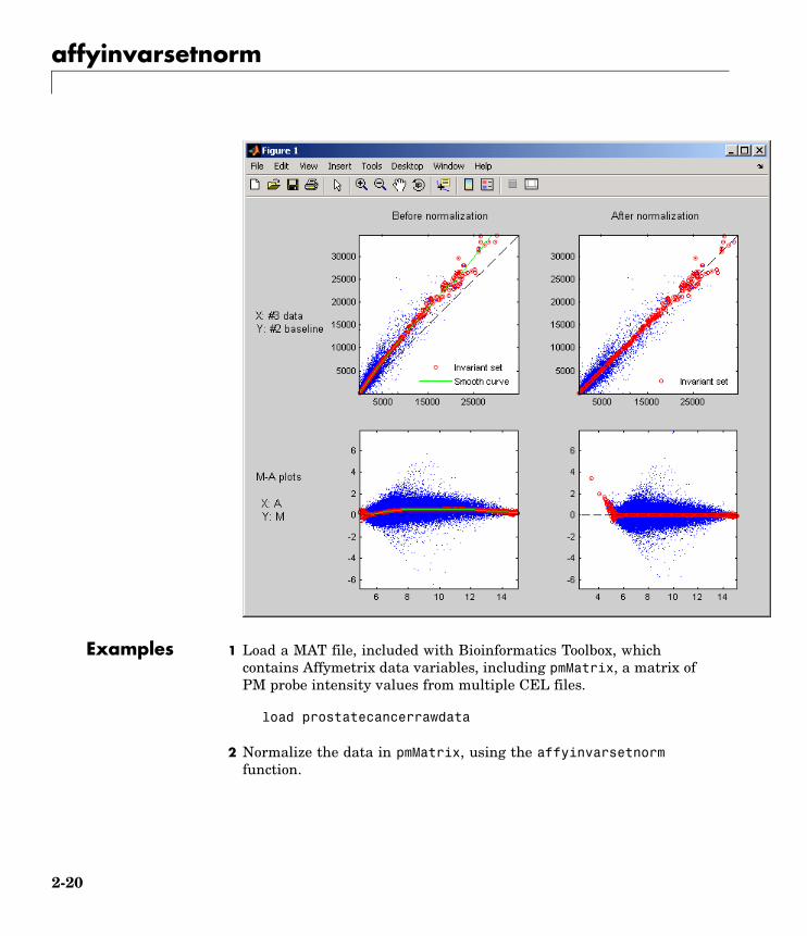
affyinvarsetnorm
Examples 1 Load a MAT file, included with Bioinformatics Toolbox, whichcontains Affymetrix data variables, including pmMatrix, a matrix ofPM probe intensity values from multiple CEL files.
load prostatecancerrawdata
2 Normalize the data in pmMatrix, using the affyinvarsetnormfunction.
2-20

affyinvarsetnorm
NormMatrix = affyinvarsetnorm(pmMatrix);
The prostatecancerrawdata.mat file used in the previous examplecontains data from Best et al., 2005.
References [1] Li, C., and Wong, W.H. (2001). Model-based analysis ofoligonucleotide arrays: model validation, design issues and standarderror application. Genome Biology 2(8): research0032.1-0032.11.
[2] http://biosun1.harvard.edu/complab/dchip/normalizing%20arrays.htm#isn
[3] Best, C.J.M., Gillespie, J.W., Yi, Y., Chandramouli, G.V.R.,Perlmutter, M.A., Gathright, Y., Erickson, H.S., Georgevich, L., Tangrea,M.A., Duray, P.H., Gonzalez, S., Velasco, A., Linehan, W.M., Matusik,R.J., Price, D.K., Figg, W.D., Emmert-Buck, M.R., and Chuaqui, R.F.(2005). Molecular alterations in primary prostate cancer after androgenablation therapy. Clinical Cancer Research 11, 6823-6834.
See Also affyread, celintensityread, mainvarsetnorm, malowess, manorm,quantilenorm, rmabackadj, rmasummary
2-21

affyprobeaffinities
Purpose Compute Affymetrix probe affinities from their sequences and MMprobe intensities
Syntax [AffinPM, AffinMM] = affyprobeaffinities(SequenceMatrix,MMIntensity)
[AffinPM, AffinMM,BaseProf] = affyprobeaffinities(SequenceMatrix,MMIntensity)
[AffinPM, AffinMM, BaseProf,Stats] = affyprobeaffinities(SequenceMatrix, MMIntensity)
... = affyprobeaffinities(SequenceMatrix, MMIntensity,
...'ProbeIndices', ProbeIndicesValue, ...)
... = affyprobeaffinities(SequenceMatrix, MMIntensity,...'Showplot', ShowplotValue, ...)
2-22

affyprobeaffinities
ArgumentsSequenceMatrix An N-by-25 matrix of sequence information for
the perfect match (PM) probes on an AffymetrixGeneChip array, where N is the number ofprobes on the array. Each row corresponds toa probe, and each column corresponds to oneof the 25 sequence positions. Nucleotides inthe sequences are represented by one of thefollowing integers:
• 0 — None
• 1 — A
• 2 — C
• 3 — G
• 4 — T
Tip You can use the affyprobeseqreadfunction to generate this matrix. If youhave this sequence information in letterrepresentation, you can convert it to integerrepresentation using the nt2int function.
MMIntensity Column vector containing mismatch (MM)probe intensities from a CEL file, generatedfrom a single Affymetrix GeneChip array. Eachrow corresponds to a probe.
Tip You can extract this column vector fromthe MMIntensities matrix returned by thecelintensityread function.
2-23

affyprobeaffinities
ProbeIndicesValue Column vector containing probe indexinginformation. Probes within a probe set arenumbered 0 through N - 1, where N is thenumber of probes in the probe set.
Tip You can use the affyprobeseqreadfunction to generate this column vector.
ShowplotValue Controls the display of a plot showing theaffinity values of each of the four bases (A, C, G,and T) for each of the 25 sequence positions, forall probes on the Affymetrix GeneChip array.Choices are true or false (default).
ReturnValues
AffinPM Column vector of PM probe affinities, computedfrom their probe sequences and MM probeintensities.
AffinMM Column vector of MM probe affinities, computedfrom their probe sequences and MM probeintensities.
Description [AffinPM, AffinMM] = affyprobeaffinities(SequenceMatrix,MMIntensity) returns a column vector of PM probe affinities and acolumn vector of MM probe affinities, computed from their probesequences and MM probe intensities. Each row in AffinPM and AffinMMcorresponds to a probe. NaN is returned for probes with no sequenceinformation. Each probe affinity is the sum of position-dependent baseaffinities. For a given base type, the positional effect is modeled as apolynomial of degree 3.
[AffinPM, AffinMM, BaseProf] =affyprobeaffinities(SequenceMatrix, MMIntensity)also estimates affinity coefficients using multiple linear regression. It
2-24

affyprobeaffinities
returns BaseProf, a 4-by-4 matrix containing the four parametersfor a polynomial of degree 3, for each base, A, C, G, and T. Each rowcorresponds to a base, and each column corresponds to a parameter.These values are estimated from the probe sequences and intensities,and represent all probes on an Affymetrix GeneChip array.
[AffinPM, AffinMM, BaseProf, Stats] =affyprobeaffinities(SequenceMatrix, MMIntensity) also returnsStats, a row vector containing four statistics in the following order:
• R-square statistic
• F statistic
• p value
• error variance
... = affyprobeaffinities(SequenceMatrix, MMIntensity,
...'PropertyName', PropertyValue, ...) callsaffyprobeaffinities with optional properties that useproperty name/property value pairs. You can specify one or moreproperties in any order. Each PropertyName must be enclosed in singlequotation marks and is case insensitive. These property name/propertyvalue pairs are as follows:
... = affyprobeaffinities(SequenceMatrix, MMIntensity,
...'ProbeIndices', ProbeIndicesValue, ...) uses probe indices tonormalize the probe intensities with the median of their probe setintensities.
Tip Use of the ProbeIndices property is recommended only if yourMMIntensity data are not from a nonspecific binding experiment.
... = affyprobeaffinities(SequenceMatrix, MMIntensity,
...'Showplot', ShowplotValue, ...) controls the display of a plot ofthe probe affinity base profile. Choices are true or false (default).
2-25

affyprobeaffinities
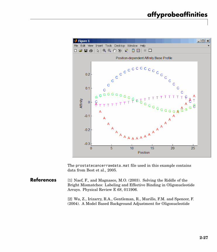
Examples 1 Load the MAT file, included with Bioinformatics Toolbox, thatcontains Affymetrix data from a prostate cancer study. The variablesin the MAT file include seqMatrix, a matrix containing sequenceinformation for PM probes, mmMatrix, a matrix containing MM probeintensity values, and probeIndices, a column vector containingprobe indexing information.
load prostatecancerrawdata
2 Compute the Affymetrix PM and MM probe affinities from theirsequences and MM probe intensities, and also plot the affinity valuesof each of the four bases (A, C, G, and T) for each of the 25 sequencepositions, for all probes on the Affymetrix GeneChip array.
[apm, amm] = affyprobeaffinities(seqMatrix, mmMatrix(:,1),...'ProbeIndices', probeIndices, 'showplot', true);
2-26
affyprobeaffinities
The prostatecancerrawdata.mat file used in this example containsdata from Best et al., 2005.
References [1] Naef, F., and Magnasco, M.O. (2003). Solving the Riddle of theBright Mismatches: Labeling and Effective Binding in OligonucleotideArrays. Physical Review E 68, 011906.
[2] Wu, Z., Irizarry, R.A., Gentleman, R., Murillo, F.M. and Spencer, F.(2004). A Model Based Background Adjustment for Oligonucleotide
2-27
affyprobeaffinities
Expression Arrays. Journal of the American Statistical Association99(468), 909–917.
[3] Best, C.J.M., Gillespie, J.W., Yi, Y., Chandramouli, G.V.R.,Perlmutter, M.A., Gathright, Y., Erickson, H.S., Georgevich, L., Tangrea,M.A., Duray, P.H., Gonzalez, S., Velasco, A., Linehan, W.M., Matusik,R.J., Price, D.K., Figg, W.D., Emmert-Buck, M.R., and Chuaqui, R.F.(2005). Molecular alterations in primary prostate cancer after androgenablation therapy. Clinical Cancer Research 11, 6823–6834.
See Also Bioinformatics Toolbox functions: affyprobeseqread, affyread,celintensityread, probelibraryinfo
2-28
affyprobeseqread
Purpose Read data file containing probe sequence information for AffymetrixGeneChip array
Syntax Struct = affyprobeseqread(SeqFile, CDFFile)Struct = affyprobeseqread(SeqFile, CDFFile, ...'SeqPath',SeqPathValue, ...)Struct = affyprobeseqread(SeqFile, CDFFile, ...'CDFPath',
CDFPathValue, ...)Struct = affyprobeseqread(SeqFile, CDFFile, ...'SeqOnly',
SeqOnlyValue, ...)
2-29

affyprobeseqread
Arguments SeqFile String specifying a file name of a sequence file(tab-separated or FASTA) that contains the followinginformation for a specific type of AffymetrixGeneChip array:
• Probe set IDs
• Probe x-coordinates
• Probe y-coordinates
• Probe sequences in each probe set
• Affymetrix GeneChip array type (FASTA file only)
The sequence file (tab-separated or FASTA) mustbe on the MATLAB search path or in the CurrentDirectory (unless you use the SeqPath property). Ina tab-separated file, each row represents a probe; ina FASTA file, each header represents a probe.
CDFFile Either of the following:
• String specifying a file name of an AffymetrixCDF library file, which contains information thatspecifies which probe set each probe belongs to ona specific type of Affymetrix GeneChip array. TheCDF library file must be on the MATLAB searchpath or in the MATLAB Current Directory (unlessyou use the CDFPath property).
• CDF structure, such as returned by the affyreadfunction, which contains information that specifieswhich probe set each probe belongs to on a specifictype of Affymetrix GeneChip array.
Caution Make sure that SeqFile and CDFFilecontain information for the same type of AffymetrixGeneChip array.
2-30
affyprobeseqread
SeqPathValue String specifying a directory or path and directorywhere SeqFile is stored.
CDFPathValue String specifying a directory or path and directorywhere CDFFile is stored.
SeqOnlyValue Controls the return of a structure, Struct, withonly one field, SequenceMatrix. Choices are trueor false (default).
ReturnValues
Struct MATLAB structure containing the following fields:• ProbeSetIDs
• ProbeIndices
• SequenceMatrix
Description Struct = affyprobeseqread(SeqFile, CDFFile) reads the data fromfiles SeqFile and CDFFile, and stores the data in the MATLABstructure Struct, which contains the following fields.
Field Description
ProbeSetIDs Cell array containing the probe set IDs from theAffymetrix CDF library file.
2-31

affyprobeseqread
Field Description
ProbeIndices Column vector containing probe indexinginformation. Probes within a probe set arenumbered 0 through N - 1, where N is the numberof probes in the probe set.
SequenceMatrix An N-by-25 matrix of sequence information forthe perfect match (PM) probes on the AffymetrixGeneChip array, where N is the number of probeson the array. Each row corresponds to a probe,and each column corresponds to one of the 25sequence positions. Nucleotides in the sequencesare represented by one of the following integers:
• 0 — None
• 1 — A
• 2 — C
• 3 — G
• 4 — T
Note Probes without sequence informationare represented in SequenceMatrix as a rowcontaining all 0s.
Tip You can use the int2nt function to convert thenucleotide sequences in SequenceMatrix to letterrepresentation.
Struct = affyprobeseqread(SeqFile, CDFFile,...'PropertyName', PropertyValue, ...) calls affyprobeseqreadwith optional properties that use property name/property value pairs.
2-32

affyprobeseqread
You can specify one or more properties in any order. Each PropertyNamemust be enclosed in single quotation marks and is case insensitive.These property name/property value pairs are as follows:
Struct = affyprobeseqread(SeqFile, CDFFile, ...'SeqPath',SeqPathValue, ...) lets you specify a path and directory whereSeqFile is stored.
Struct = affyprobeseqread(SeqFile, CDFFile, ...'CDFPath',CDFPathValue, ...) lets you specify a path directory where CDFFileis stored.
Struct = affyprobeseqread(SeqFile, CDFFile, ...'SeqOnly',SeqOnlyValue, ...) controls the return of a structure, Struct, withonly one field, SequenceMatrix. Choices are true or false (default).
Examples 1 Read the data from a FASTA file and associated CDF library file,assuming both are located on the MATLAB search path or in theCurrent Directory.
S1 = affyprobeseqread('HG-U95A_probe_fasta', 'HG_U95A.CDF');
2 Read the data from a tab-separated file and associated CDFstructure, assuming the tab-separated file is located in the specifieddirectory and the CDF structure is in your MATLAB Workspace.
S2 = affyprobeseqread('HG-U95A_probe_tab',hgu95aCDFStruct,...'seqpath','C:\Affymetrix\SequenceFiles\HGGenome');
3 Access the nucleotide sequences of the first probe set (rows 1 through20) in the SequenceMatrix field of the S2 structure.
seq = int2nt(S2.SequenceMatrix(1:20,:))
See Also Bioinformatics Toolbox functions: affyinvarsetnorm, affyread,celintensityread, int2nt, probelibraryinfo, probesetlink,probesetlookup, probesetplot, probesetvalues
2-33

affyread
Purpose Read microarray data from Affymetrix GeneChip file (Windows 32)
Syntax AffyStruct = affyread(File)AffyStruct = affyread(File, LibraryPath)
2-34

affyread
Arguments File String specifying a file name or a path and file nameof one of the following Affymetrix file types:• DAT — Data file containing raw image data.
• CEL — Data file containing information about theexpression levels of the individual probes.
• CHP — Data file containing information aboutprobe sets.
• EXP — Data file containing information aboutexperimental conditions and protocols.
• CDF — Library file containing information aboutwhich probes belong to which probe set.
• GIN — Library file containing information aboutthe probe sets, such as the gene name with whichthe probe set is associated.
If you specify only a file name, that file must be onthe MATLAB search path or in the MATLAB CurrentDirectory.
LibraryPath String specifying the path and directory where thelibrary file (CDF or GIN) associated with File isstored.
Note This input argument is needed only if File isa CHP file.
2-35

affyread
ReturnValues
AffyStruct MATLAB structure containing information from theAffymetrix data or library file.
DescriptionNote This function is supported on the Windows 32 platform only.
AffyStruct = affyread(File) reads File, an Affymetrix file, andcreates AffyStruct, a MATLAB structure.
AffyStruct contains the following fields:
AffyStruct = affyread(File, LibraryPath) specifies the path anddirectory where the library file (CDF or GIN) associated with File isstored. Use this syntax only if File is a CHP file.
You can learn more about the Affymetrix GeneChip files and downloadsample files from:
http://www.affymetrix.com/support/technical/sample_data/demo_data.affx
Note Some Affymetrix sample data files (DAT, EXP, CEL, and CHP)are combined together in a DTT file. You must download and use theAffymetrix Data Transfer Tool to extract these files from the DTT file.
2-36

affyread
Caution
When using affyread to read a CHP file, the Affymetrix GDACRuntime Libraries look for the associated CEL file in the directory thatit was in when the CHP file was created. If the CEL file is not found,then affyread does not read probe set values in the CHP file.
If you encounter errors reading files, then check that the AffymetrixGDAC Runtime Libraries are correctly installed. You can reinstall thelibraries by running the installer from Windows Explorer:
$MATLAB$\toolbox\bioinfo\microarray\lib\...GdacFilesRuntimeInstall-v4.exe
Examples The following example assumes that Drosophila.CEL andDrosophila.dat are stored on the MATLAB search path or in theMATLAB Current Directory. It also assumes that Drosophila.chpis stored on the MATLAB search path or in the MATLABCurrent Directory, and that its associated library file is stored atD:\Affymetrix\LibFiles\DrosGenome1.
1 Read the contents of a CEL file into a MATLAB structure.
celStruct = affyread('Drosophila.CEL')
2 Display a spatial plot of the probe intensities.
maimage(celStruct, 'Intensity')
3 Read the contents of a DAT file into a MATLAB structure, and thendisplay the raw image data.
datStruct = affyread('Drosophila.dat')imagesc(datStruct.Image);axis image;
2-37
affyread
4 Read the contents of a CHP file into a MATLAB structure, and thenplot the probe values for a probe set. The CHP files require the libraryfiles. Your file may be in a different location than this example.
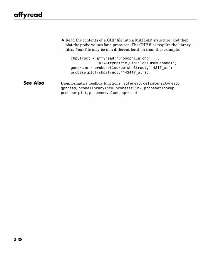
chpStruct = affyread('Drosophila.chp',...'D:\Affymetrix\LibFiles\DrosGenome1')
geneName = probesetlookup(chpStruct,'14317_at')probesetplot(chpStruct,'142417_at');
See Also Bioinformatics Toolbox functions: agferead, celintensityread,gprread, probelibraryinfo, probesetlink, probesetlookup,probesetplot, probesetvalues, sptread
2-38
agferead
Purpose Read Agilent Feature Extraction Software file
Syntax AGFEData = agferead(File)
ArgumentsFile Microarray data file generated with the Agilent
Feature Extraction Software.
Description AGFEData = agferead(File) reads files generated with FeatureExtraction Software from Agilent micoararry scanners and creates astructure (AGFEData) containing the following fields:
• Header
• Stats
• Columns
• Rows
• Names
• IDs
• Data
• ColumnNames
• TextData
• TextColumnNames
Feature Extraction Software takes an image from an Agilent microarrayscanner and generates raw intensity data for each spot on the plate.For more information about this software, see a description on theirWeb site at
http://www.chem.agilent.com/scripts/pds.asp?lpage=2547
Examples 1 Read in a sample Agilent Feature Extraction Software file. Note thatthe file fe_sample.txt is not provided with Bioinformatics Toolbox.
2-39
agferead
agfeStruct = agferead('fe_sample.txt')
2 Plot the median foreground.
maimage(agfeStruct,'gMedianSignal');maboxplot(agfeStruct,'gMedianSignal');
See Also Bioinformatics Toolbox functions: affyread, celintensityread,galread, geosoftread, gprread, imageneread, magetfield, sptread
2-40
aminolookup
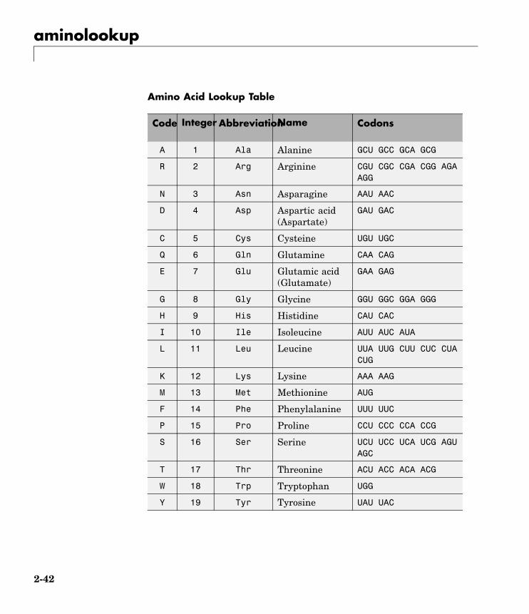
Purpose Find amino acid codes, integers, abbreviations, names, and codons
Syntax aminolookupaminolookup(SeqAA)aminolookup('Code', CodeValue)aminolookup('Integer', IntegerValue)aminolookup('Abbreviation', AbbreviationValue)aminolookup('Name', NameValue)
Arguments SeqAA Character string of single-letter codes orthree-letter abbreviations representing anamino acid sequence. See the Amino AcidLookup Table on page 2-42 for valid codes andabbreviations.
CodeValue String specifying a single-letter representingan amino acid. See the Amino Acid LookupTable on page 2-42 for valid single-letter codes.
IntegerValue Single integer representing an amino acid. Seethe Amino Acid Lookup Table on page 2-42 forvalid integers.
AbbreviationValue String specifying a three-letter abbreviationrepresenting an amino acid. See the AminoAcid Lookup Table on page 2-42 for validthree-letter abbreviations.
NameValue String specifying an amino acid name. Seethe Amino Acid Lookup Table on page 2-42 forvalid amino acid names.
2-41
aminolookup
Amino Acid Lookup Table
Code Integer AbbreviationName Codons
A 1 Ala Alanine GCU GCC GCA GCG
R 2 Arg Arginine CGU CGC CGA CGG AGAAGG
N 3 Asn Asparagine AAU AAC
D 4 Asp Aspartic acid(Aspartate)
GAU GAC
C 5 Cys Cysteine UGU UGC
Q 6 Gln Glutamine CAA CAG
E 7 Glu Glutamic acid(Glutamate)
GAA GAG
G 8 Gly Glycine GGU GGC GGA GGG
H 9 His Histidine CAU CAC
I 10 Ile Isoleucine AUU AUC AUA
L 11 Leu Leucine UUA UUG CUU CUC CUACUG
K 12 Lys Lysine AAA AAG
M 13 Met Methionine AUG
F 14 Phe Phenylalanine UUU UUC
P 15 Pro Proline CCU CCC CCA CCG
S 16 Ser Serine UCU UCC UCA UCG AGUAGC
T 17 Thr Threonine ACU ACC ACA ACG
W 18 Trp Tryptophan UGG
Y 19 Tyr Tyrosine UAU UAC
2-42
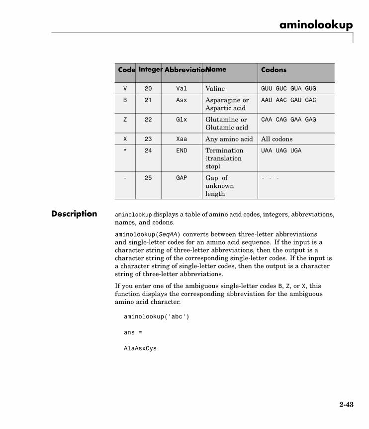
aminolookup
Code Integer AbbreviationName Codons
V 20 Val Valine GUU GUC GUA GUG
B 21 Asx Asparagine orAspartic acid
AAU AAC GAU GAC
Z 22 Glx Glutamine orGlutamic acid
CAA CAG GAA GAG
X 23 Xaa Any amino acid All codons
* 24 END Termination(translationstop)
UAA UAG UGA
- 25 GAP Gap ofunknownlength
- - -
Description aminolookup displays a table of amino acid codes, integers, abbreviations,names, and codons.
aminolookup(SeqAA) converts between three-letter abbreviationsand single-letter codes for an amino acid sequence. If the input is acharacter string of three-letter abbreviations, then the output is acharacter string of the corresponding single-letter codes. If the input isa character string of single-letter codes, then the output is a characterstring of three-letter abbreviations.
If you enter one of the ambiguous single-letter codes B, Z, or X, thisfunction displays the corresponding abbreviation for the ambiguousamino acid character.
aminolookup('abc')
ans =
AlaAsxCys
2-43
aminolookup
aminolookup('Code', CodeValue) displays the corresponding aminoacid three-letter abbreviation and name.
aminolookup('Integer', IntegerValue) displays the correspondingamino acid single-letter code, three-letter abbreviation, and name.
aminolookup('Abbreviation', AbbreviationValue) displays thecorresponding amino acid single-letter code and name.
aminolookup('Name', NameValue) displays the corresponding aminoacid single-letter code and three-letter abbreviation.
Examples 1 Convert an amino acid sequence in single-letter codes to thecorresponding three-letter abbreviations.
aminolookup('MWKQAEDIRDIYDF')
ans =
MetTrpLysGlnAlaGluAspIleArgAspIleTyrAspPhe
2 Convert an amino acid sequence in three-letter abbreviations to thecorresponding single-letter codes.
aminolookup('MetTrpLysGlnAlaGluAspIleArgAspIleTyrAspPhe')
ans =
MWKQAEDIRDIYDF
3 Display the three-letter abbreviation and name for the amino acidcorresponding to the single-letter code R.
aminolookup('code', 'R')
ans =
Arg Arginine
2-44

aminolookup
4 Display the single-letter code, three-letter abbreviation, and namefor the amino acid corresponding to the integer 1.
aminolookup('integer', 1)
ans =
A Ala Alanine
5 Display the single-letter code and name for the amino acidcorresponding to the three-letter abbreviation asn.
aminolookup('abbreviation', 'asn')
ans =
N Asparagine
6 Display the single-letter code and three-letter abbreviation for theamino acid proline.
aminolookup('Name','proline')
ans =
P Pro
See Also Bioinformatics Toolbox functions: aa2int, aacount, geneticcode,int2aa, nt2aa, revgeneticcode
2-45

atomiccomp
Purpose Calculate atomic composition of protein
Syntax NumberAtoms = atomiccomp(SeqAA)
ArgumentsSeqAA Amino acid sequence. Enter a character string or vector
of integers from the table . You can also enter a structurewith the field Sequence.
Description NumberAtoms = atomiccomp(SeqAA) counts the type and number ofatoms in an amino acid sequence (SeqAA) and returns the counts in a1-by-1 structure (NumberAtoms) with fields C, H, N, O, and S.
Examples 1 Get an amino acid sequence from the NCBI Genpept Database.
rhodopsin = getgenpept('NP_000530');
2 Count the atoms in a sequence.
rhodopsinAC = atomiccomp(rhodopsin)
rhodopsinAC =
C: 1814H: 2725N: 423O: 477S: 25
3 Retrieve the number of carbon atoms in the sequence.
rhodopsinAC.C
ans =
1814
2-46

atomiccomp
See Also Bioinformatics Toolbox functions aacount, molweight, proteinplot
2-47

basecount
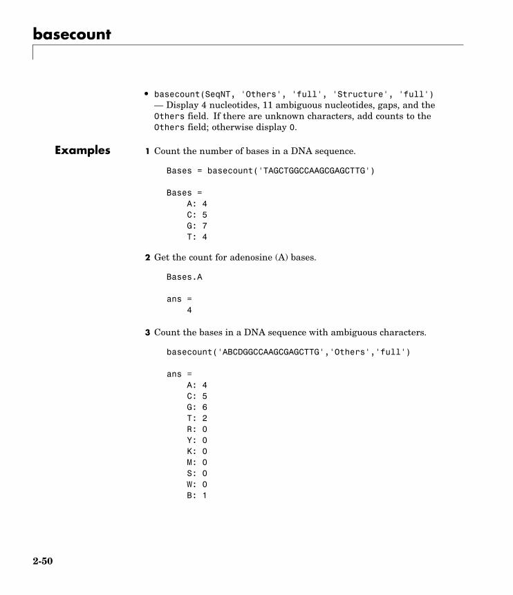
Purpose Count nucleotides in sequence
Syntax NumberBases = basecount(SeqNT)basecount(..., 'PropertyName', PropertyValue,...)basecount(..., 'Chart', ChartValue)basecount(..., 'Others', OthersValue)basecount(..., 'Structure', StructureValue),
ArgumentsSeqNT Nucleotide sequence. Enter a character string
with the letters A, T, U, C, and G. The count forU characters is included with the count for Tcharacters. . You can also enter a structure withthe field Sequence.
ChartValue Property to select a type of plot. Enter either 'pie'or 'bar'.
OthersValue Property to control counting ambiguous charactersindividually. Enter either full' or 'bundle'(default).
Description NumberBases = basecount(SeqNT) counts the number of bases in anucleotide sequence (SeqNT) and returns the base counts in a 1-by-1structure (Bases) with the fields A, C, G, T.
• For sequences with the character U, the number of U characters isadded to the number of T characters.
• If a sequence contains ambiguous nucleotide characters (R, Y, K, M,S, W, B, D, H, V, N), or gaps indicated with a hyphen (-), this functioncreates a field Others and displays a warning message.
Warning: Ambiguous symbols 'symbol list' appearin the sequence.These will be in Others.
2-48

basecount
• If a sequence contains undefined nucleotide characters (E F H I JL O P Q X Z) , the characters are counted in the field Others and awarning message is displayed.
Warning: Unknown symbols 'symbol list' appearin the sequence.These will be ignored.
• If the property Others = 'full', ambiguous characters are listedseparately and hyphens are counted in a new field (Gaps).
basecount(..., 'PropertyName', PropertyValue,...) definesoptional properties using property name/value pairs:
basecount(..., 'Chart', ChartValue) creates a chart showing therelative proportions of the nucleotides.
basecount(..., 'Others', OthersValue), when OthersValue is'full', counts all the ambiguous nucleotide symbols individuallyinstead of bundling them together into the Others field of the outputstructure.
basecount(..., 'Structure', StructureValue), whenStructureValue is 'full' , blocks the unknown characters warningand ignores counting unknown characters.
• basecount(SeqNT) — Display four nucleotides, and only if thereare ambiguous and unknown characters, add an Others field withthe counts.
• basecount(SeqNT, 'Others', 'full') — Display four nucleotides,11 ambiguous nucleotides, gaps, and only if there are unknowncharacters, add an Others field with the unknown counts.
• basecount(SeqNT, 'Structure', 'full') — Display fournucleotides and always display an Others field. If there areambiguous and unknown characters, add counts to the Others field;otherwise display 0.
2-49
basecount
• basecount(SeqNT, 'Others', 'full', 'Structure', 'full')— Display 4 nucleotides, 11 ambiguous nucleotides, gaps, and theOthers field. If there are unknown characters, add counts to theOthers field; otherwise display 0.
Examples 1 Count the number of bases in a DNA sequence.
Bases = basecount('TAGCTGGCCAAGCGAGCTTG')
Bases =A: 4C: 5G: 7T: 4
2 Get the count for adenosine (A) bases.
Bases.A
ans =4
3 Count the bases in a DNA sequence with ambiguous characters.
basecount('ABCDGGCCAAGCGAGCTTG','Others','full')
ans =A: 4C: 5G: 6T: 2R: 0Y: 0K: 0M: 0S: 0W: 0B: 1
2-50

basecount
D: 1H: 0V: 0N: 0
Gaps: 0
See Also Bioinformatics Toolbox functions aacount, baselookup, codoncount,cpgisland, dimercount, nmercount, ntdensity, seqtool
2-51

baselookup
Purpose Nucleotide codes, abbreviations, and names
Syntax baselookup('Complement', SeqNT)baselookup('Code', CodeValue)baselookup('Integer', IntegerValue)baselookup('Name', NameValue)
Arguments SeqNT Nucleotide sequence. Enter a character string ofsingle-letter codes from the Nucleotide LookupTable below.
In addition to a single nucleotide sequence,SeqNT can be a cell array of sequences,or a two-dimensional character array ofsequences. The complement for each sequenceis determined independently.
CodeValue Nucleotide letter code. Enter a single characterfrom the Nucleotide Lookup Table below. Codecan also be a cell array or a two-dimensionalcharacter array.
IntegerValue Nucleotide integer. Enter an integer from theNucleotide Lookup Table below. Integers arearbitrarily assigned to IUB/IUPAC letters.
NameValue Nucleotide name. Enter a nucleotide name fromthe Nucleotide Lookup Table below. NameValuecan also be a single name, a cell array, or atwo-dimensional character array.
Nucleotide Lookup Table
Code Integer Base Name Meaning Complement
A 1 Adenine A T
C 2 Cytosine C G
2-52
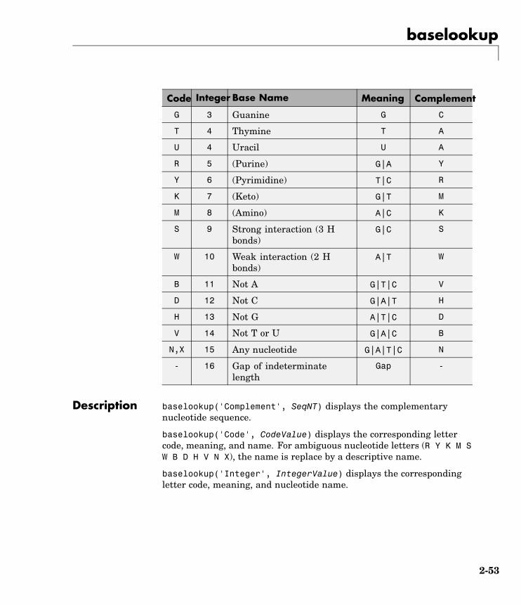
baselookup
Code Integer Base Name Meaning Complement
G 3 Guanine G C
T 4 Thymine T A
U 4 Uracil U A
R 5 (Purine) G|A Y
Y 6 (Pyrimidine) T|C R
K 7 (Keto) G|T M
M 8 (Amino) A|C K
S 9 Strong interaction (3 Hbonds)
G|C S
W 10 Weak interaction (2 Hbonds)
A|T W
B 11 Not A G|T|C V
D 12 Not C G|A|T H
H 13 Not G A|T|C D
V 14 Not T or U G|A|C B
N,X 15 Any nucleotide G|A|T|C N
- 16 Gap of indeterminatelength
Gap -
Description baselookup('Complement', SeqNT) displays the complementarynucleotide sequence.
baselookup('Code', CodeValue) displays the corresponding lettercode, meaning, and name. For ambiguous nucleotide letters (R Y K M SW B D H V N X), the name is replace by a descriptive name.
baselookup('Integer', IntegerValue) displays the correspondingletter code, meaning, and nucleotide name.
2-53

baselookup
baselookup('Name', NameValue) displays the corresponding lettercode and meaning.
Examples baselookup('Complement', 'TAGCTGRCCAAGGCCAAGCGAGCTTN')
baselookup('Name','cytosine')
See Also Bioinformatics Toolbox functions basecount, codoncount, dimercount,geneticcode, nt2aa, nt2int, revgeneticcode, seqtool
2-54

biograph
Purpose Create biograph object
Syntax BGobj = biograph(CMatrix)BGobj = biograph(CMatrix, NodeIDs)BGobj = biograph(CMatrix, NodeIDs, ...'ID', IDValue, ...)BGobj = biograph(CMatrix, NodeIDs, ...'Label', LabelValue,
...)BGobj = biograph(CMatrix, NodeIDs, ...'Description',
DescriptionValue, ...)BGobj = biograph(CMatrix, NodeIDs, ...'LayoutType',
LayoutTypeValue, ...)BGobj = biograph(CMatrix, NodeIDs, ...'EdgeType',
EdgeTypeValue, ...)BGobj = biograph(CMatrix, NodeIDs, ...'Scale', ScaleValue,
...)BGobj = biograph(CMatrix, NodeIDs, ...'LayoutScale',
LayoutScaleValue, ...)BGobj = biograph(CMatrix, NodeIDs, ...'EdgeTextColor',
EdgeTextColorValue, ...)BGobj = biograph(CMatrix, NodeIDs, ...'EdgeFontSize',
EdgeFontSizeValue, ...)BGobj = biograph(CMatrix, NodeIDs, ...'ShowArrows',
ShowArrowsValue, ...)BGobj = biograph(CMatrix, NodeIDs, ...'ArrowSize',
ArrowSizeValue, ...)BGobj = biograph(CMatrix, NodeIDs, ...'ShowWeights',
ShowWeightsValue, ...)BGobj = biograph(CMatrix, NodeIDs, ...'ShowTextInNodes',
ShowTextInNodesValue, ...)BGobj = biograph(CMatrix, NodeIDs, ...'NodeAutoSize',
NodeAutoSizeValue, ...)BGobj = biograph(CMatrix, NodeIDs, ...'NodeCallback',
NodeCallbackValue, ...)BGobj = biograph(CMatrix, NodeIDs, ...'EdgeCallback',
EdgeCallbackValue, ...)BGobj = biograph(CMatrix, NodeIDs, ...'CustomNodeDrawFcn',
CustomNodeDrawFcnValue, ...)
2-55

biograph
ArgumentsCMatrix Full or sparse square matrix that acts as
a connection matrix. That is, a value of1 indicates a connection between nodeswhile a 0 indicates no connection. Thenumber of rows/columns is equal to thenumber of nodes.
NodeIDs Node identification strings. Enter any ofthe following:• Cell array of strings with the number
of strings equal to the number of rowsor columns in the connection matrixCMatrix. Each string must be unique.
• Character array with the number ofrows equal to the number of nodes.Each row in the array must be unique.
• String with the number of charactersequal to the number of nodes. Eachcharacter must be unique.
Default values are the row or columnnumbers.
Note You must specify NodeIDs if youwant to specify property name/valuepairs. Set NodeIDs to [] to use the defaultvalues of the row/column numbers.
IDValue String to identify the biograph object.Default is ''. (This information is forbookkeeping purposes only.)
2-56

biograph
LabelValue String to label the biograph object.Default is ''. (This information is forbookkeeping purposes only.)
DescriptionValue String that describes the biograph object.Default is ''. (This information is forbookkeeping purposes only.)
LayoutTypeValue String that specifies the algorithm for thelayout engine. Choices are:• 'hierarchical' (default)
• 'equilibrium'
• 'radial'
EdgeTypeValue String that specifies how edges display.Choices are:• 'straight'
• 'curved' (default)
• 'segmented'
Note Curved or segmented edgesoccur only when necessary to avoidobstruction by nodes. Biograph objectswith LayoutType equal to 'equilibrium'or 'radial' cannot produce curved orsegmented edges.
ScaleValue Positive number that post-scales the nodecoordinates. Default is 1.
LayoutScaleValue Positive number that scales the size of thenodes before calling the layout engine.Default is 1.
2-57
biograph
EdgeTextColorValue Three-element numeric vector of RGBvalues. Default is [0, 0, 0], whichdefines black.
EdgeFontSizeValue Positive number that sets the size of theedge font in points. Default is 8.
ShowArrowsValue Controls the display of arrows for theedges. Choices are 'on' (default) or'off'.
ArrowSizeValue Positive number that sets the size of thearrows in points. Default is 8.
ShowWeightsValue Controls the display of text indicating theweight of the edges. Choices are 'on'(default) or 'off'.
ShowTextInNodesValue String that specifies the node propertyused to label nodes when you display abiograph object using the view method.Choices are:
• 'Label' — Uses the Label property ofthe node object (default).
• 'ID' — Uses the ID property of thenode object.
• 'None'
2-58

biograph
NodeAutoSizeValue Controls precalculating the node sizebefore calling the layout engine. Choicesare 'on' (default) or 'off'.
NodeCallbackValue User callback for all nodes. Enter thename of a function, a function handle, or acell array with multiple function handles.After using the view function to displaythe biograph in the Biograph Viewer, youcan double-click a node to activate thefirst callback, or right-click and select acallback to activate. Default is @(node)inspect(node), which displays theProperty Inspector dialog box.
EdgeCallbackValue User callback for all edges. Enter thename of a function, a function handle, or acell array with multiple function handles.After using the view function to displaythe biograph in the Biograph Viewer, youcan double-click an edge to activate thefirst callback, or right-click and select acallback to activate. Default is @(edge)inspect(edge), which displays theProperty Inspector dialog box.
CustomNodeDrawFcnValue Function handle to customized function todraw nodes. Default is [].
Description BGobj = biograph(CMatrix) creates a biograph object, BGobj, using aconnection matrix, CMatrix. All nondiagonal and positive entries in theconnection matrix, CMatrix, indicate connected nodes, rows representthe source nodes, and columns represent the sink nodes.
BGobj = biograph(CMatrix, NodeIDs) specifies the nodeidentification strings. NodeIDs can be:
2-59

biograph
• Cell array of strings with the number of strings equal to the numberof rows or columns in the connection matrix CMatrix. Each stringmust be unique.
• Character array with the number of rows equal to the number ofnodes. Each row in the array must be unique.
• String with the number of characters equal to the number of nodes.Each character must be unique.
Default values are the row or column numbers.
Note If you want to specify property name/value pairs, you mustspecify NodeIDs. Set NodeIDs to [] to use the default values of therow/column numbers.
BGobj = biograph(..., 'PropertyName', PropertyValue, ...)calls biograph with optional properties that use property name/propertyvalue pairs. You can specify one or more properties in any order. EachPropertyName must be enclosed in single quotation marks and is caseinsensitive. These property name/property value pairs are as follows:
BGobj = biograph(CMatrix, NodeIDs, ...'ID', IDValue, ...) specifiesan ID for the biograph object. Default is ''. (This information is forbookkeeping purposes only.)
BGobj = biograph(CMatrix, NodeIDs, ...'Label', LabelValue, ...)specifies a label for the biograph object. Default is ''. (This informationis for bookkeeping purposes only.)
BGobj = biograph(CMatrix, NodeIDs, ...'Description',DescriptionValue, ...) specifies a description of the biograph object.Default is ''. (This information is for bookkeeping purposes only.)
BGobj = biograph(CMatrix, NodeIDs, ...'LayoutType',LayoutTypeValue, ...) specifies the algorithm for the layout engine.
2-60
biograph
BGobj = biograph(CMatrix, NodeIDs, ...'EdgeType', EdgeTypeValue,...) specifies how edges display.
BGobj = biograph(CMatrix, NodeIDs, ...'Scale', ScaleValue, ...)post-scales the node coordinates. Default is 1.
BGobj = biograph(CMatrix, NodeIDs, ...'LayoutScale',LayoutScaleValue, ...) scales the size of the nodes before calling thelayout engine. Default is 1.
BGobj = biograph(CMatrix, NodeIDs, ...'EdgeTextColor',EdgeTextColorValue, ...) specifies a three-element numeric vector ofRGB values. Default is [0, 0, 0], which defines black.
BGobj = biograph(CMatrix, NodeIDs, ...'EdgeFontSize',EdgeFontSizeValue, ...) sets the size of the edge font in points.Default is 8.
BGobj = biograph(CMatrix, NodeIDs, ...'ShowArrows',ShowArrowsValue, ...) controls the display of arrows for the edges.Choices are 'on' (default) or 'off'.
BGobj = biograph(CMatrix, NodeIDs, ...'ArrowSize', ArrowSizeValue,...) sets the size of the arrows in points. Default is 8.
BGobj = biograph(CMatrix, NodeIDs, ...'ShowWeights',ShowWeightsValue, ...) controls the display of text indicating theweight of the edges. Choices are 'on' (default) or 'off'.
BGobj = biograph(CMatrix, NodeIDs, ...'ShowTextInNodes',ShowTextInNodesValue, ...) specifies the node property used to labelnodes when you display a biograph object using the view method.
BGobj = biograph(CMatrix, NodeIDs, ...'NodeAutoSize',NodeAutoSizeValue, ...) controls precalculating the node size beforecalling the layout engine. Choices are 'on' (default) or 'off'.
BGobj = biograph(CMatrix, NodeIDs, ...'NodeCallback',NodeCallbackValue, ...) specifies user callback for all nodes.
BGobj = biograph(CMatrix, NodeIDs, ...'EdgeCallback',EdgeCallbackValue, ...) specifies user callback for all edges.
2-61

biograph
BGobj = biograph(CMatrix, NodeIDs, ...'CustomNodeDrawFcn',CustomNodeDrawFcnValue, ...) specifies function handle to customizedfunction to draw nodes. Default is [].
Examples 1 Create a biograph object with default node IDs, and then use the getfunction to display the node IDs.
cm = [0 1 1 0 0;1 0 0 1 1;1 0 0 0 0;0 0 0 0 1;1 0 1 0 0];bg1 = biograph(cm)Biograph object with 5 nodes and 9 edges.get(bg1.nodes,'ID')
ans =
'Node 1''Node 2''Node 3''Node 4''Node 5'
2 Create a biograph object, assign the node IDs, and then use the getfunction to display the node IDs.
cm = [0 1 1 0 0;1 0 0 1 1;1 0 0 0 0;0 0 0 0 1;1 0 1 0 0];ids = {'M30931','L07625','K03454','M27323','M15390'};bg2 = biograph(cm,ids);get(bg2.nodes,'ID')
ans =
'M30931''L07625''K03454''M27323''M15390'
3 Use the view method to display the biograph object.
2-62

biograph
view(bg2)
See Also Bioinformatics Toolbox object: biograph object
Bioinformatics Toolbox methods of a biograph object:allshortestpaths, conncomp, dolayout, getancestors,getdescendants, getedgesbynodeid, getmatrix, getnodesbyid,
2-63
biograph
getrelatives, isdag, isomorphism, isspantree, maxflow,minspantree, shortestpath, topoorder, traverse, view
MATLAB functions: get, set
2-64

blastncbi
Purpose Generate remote BLAST request
Syntax blastncbi(Seq, Program)RID = blastncbi(Seq, Program)[RID, RTOE] = blastncbi(Seq, Program)blastncbi(..., 'PropertyName', PropertyValue,...)blastncbi(..., 'Database', DatabaseValue)blastncbi(..., 'Descriptions', DescriptionsValue)blastncbi(..., 'Alignments', AlignmentsValue)blastncbi(..., 'Filter', FilterValue)blastncbi(..., 'Expect', ExpectValue)blastncbi(..., 'Word', WordValue)blastncbi(..., 'Matrix', MatrixValue)blastncbi(..., 'GapOpen', GapOpenValue)blastncbi(..., 'ExtendGap', ExtendGapValue)blastncbi(..., 'Inclusion', InclusionValue)blastncbi(..., 'Pct', PctValue)
Arguments Seq Nucleotide or amino acid sequence. Enter aGenBank or RefSeq accession number, GI,FASTA file, URL, string, character array, ora MATLAB structure that contains the fieldSequence. You can also enter a structure withthe field Sequence.
Program BLAST program. Enter 'blastn', 'blastp','psiblast', 'blastx', 'tblastn', 'tblastx',or 'megablast'.
2-65

blastncbi
DatabaseValue Property to select a database. Compatibledatabases depend upon the type of sequencesubmitted and program selected. Thenonredundant database, 'nr', is the defaultvalue for both nucleotide and amino acidsequences.
For nucleotide sequences, enter 'nr', 'est','est_human', 'est_mouse', 'est_others','gss', 'htgs', 'pat', 'pdb', 'month','alu_repeats', 'dbsts', 'chromosome', 'wgs','refseq_rna', 'refseq_genomic', or 'env_nt'.The default value is 'nr'.
For amino acid sequences, enter 'nr','swissprot', 'pat', 'pdb','month','refseq_protein', or 'env_nr', . The defaultvalue is 'nr'.
DescriptionValue Property to specify the number of shortdescriptions. The default value is normally 100,and for Program = pciblast, the default valueis 500.
AlignmentValue Property to specify the number of sequences toreport high-scoring segment pairs (HSP). Thedefault value is normally 100, and for Program =pciblast, the default value is 500.
FilterValue Property to select a filter. Enter 'L'(low-complexity), 'R' (human repeats), 'm'(mask for lookup table), or 'lcase' (to turn onthe lowercase mask). The default value is 'L'.
ExpectValue Property to select the statistical significancethreshold. Enter a real number. The defaultvalue is 10.
WordValue Property to select a word length. For amino acidsequences, Word can be 2 or 3 (3 is the defaultvalue), and for nucleotide sequences, Word can be7, 11, or 15 (11 is the default value). If Program= 'MegaBlast', Word can be 11, 12, 16, 20, 24,28, 32, 48, or 64, with a default value of 28.
2-66
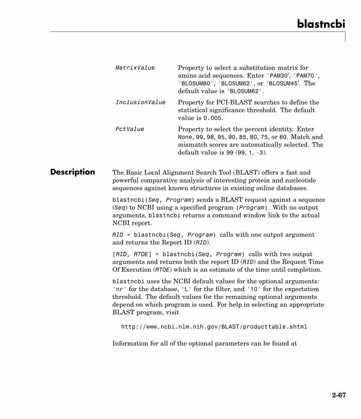
blastncbi
MatrixValue Property to select a substitution matrix foramino acid sequences. Enter 'PAM30’, 'PAM70','BLOSUM80', 'BLOSUM62', or 'BLOSUM45’. Thedefault value is 'BLOSUM62'.
InclusionValue Property for PCI-BLAST searches to define thestatistical significance threshold. The defaultvalue is 0.005.
PctValue Property to select the percent identity. EnterNone, 99, 98, 95, 90, 85, 80, 75, or 60. Match andmismatch scores are automatically selected. Thedefault value is 99 (99, 1, -3).
Description The Basic Local Alignment Search Tool (BLAST) offers a fast andpowerful comparative analysis of interesting protein and nucleotidesequences against known structures in existing online databases.
blastncbi(Seq, Program) sends a BLAST request against a sequence(Seq) to NCBI using a specified program (Program). With no outputarguments, blastncbi returns a command window link to the actualNCBI report.
RID = blastncbi(Seq, Program) calls with one output argumentand returns the Report ID (RID).
[RID, RTOE] = blastncbi(Seq, Program) calls with two outputarguments and returns both the report ID (RID) and the Request TimeOf Execution (RTOE) which is an estimate of the time until completion.
blastncbi uses the NCBI default values for the optional arguments:'nr' for the database, 'L' for the filter, and '10' for the expectationthreshold. The default values for the remaining optional argumentsdepend on which program is used. For help in selecting an appropriateBLAST program, visit
http://www.ncbi.nlm.nih.gov/BLAST/producttable.shtml
Information for all of the optional parameters can be found at
2-67

blastncbi
http://www.ncbi.nlm.nih.gov/staff/tao/URLAPI/blastcgihelp_new.html
blastncbi(..., 'PropertyName', PropertyValue,...) definesoptional properties using property name/value pairs.
blastncbi(..., 'Database', DatabaseValue) selects a databasefor the alignment search.
blastncbi(..., 'Descriptions', DescriptionsValue) , when thefunction is called without output arguments, specifies the numbers ofshort descriptions returned to the quantity specified.
blastncbi(..., 'Alignments', AlignmentsValue), when thefunction is called without output arguments, specifies the number ofsequences for which high-scoring segment pairs (HSPs) are reported.
blastncbi(..., 'Filter', FilterValue) selects the filter to appliedto the query sequence.
blastncbi(..., 'Expect', ExpectValue) provides a statisticalsignificance threshold for matches against database sequences. You canlearn more about the statistics of local sequence comparison at
http://www.ncbi.nlm.nih.gov/BLAST/tutorial/Altschul-1.html#head2
blastncbi(..., 'Word', WordValue) selects a word size for aminoacid sequences.
blastncbi(..., 'Matrix', MatrixValue) selects the substitutionmatrix for amino acid sequences only. This matrix assigns the score fora possible alignment of two amino acid residues.
blastncbi(..., 'GapOpen', GapOpenValue) selects a gap penalty foramino acid sequences. Allowable values for a gap penalty vary withthe selected substitution matrix. For information about allowed gappenalties for matrixes other then the BLOSUM62 matrix, see
http://www.ncbi.nlm.nih.gov/staff/tao/URLAPI/blastcgihelp_new.html
blastncbi(..., 'ExtendGap', ExtendGapValue) defines the penaltyfor extending a gap greater than one space.
2-68
blastncbi
blastncbi(..., 'Inclusion', InclusionValue) for PSI-BLASTonly, defines the statistical significance threshold (InclusionValue)for including a sequence in the Position Specific Score Matrix (PSSm)created by PSI-BLAST for the subsequent iteration. The default valueis 0.005.
blastncbi(..., 'Pct', PctValue), when ProgramValue is'Megablast', selects the percent identity and the correspondingmatch and mismatch score for matching existing sequences in a publicdatabase.
2-69

blastncbiV
alu
esby
Pro
gra
m
BLA
STN
BLA
STP
BLA
STX
TBLA
STN
TBLA
STX
MEG
A
Dat
abas
enr
(def
ault
),est
,est_human,
est_mouse,
est_others,
gss,htgs
,pat
,pdb,month,
alu_repeats,
dbsts,
chromosome,
wgs,
refseq_rna,
refseq_genomic,
env_nt
nr
(def
ault
),swissprot
,pat,pdb,
month
,refseq_protein,
env_nr
valu
essa
me
asB
LA
ST
Pva
lues
sam
eas
BL
AS
TN
valu
essa
me
asB
LA
ST
Nva
lues
sam
eas
BL
AS
TN
Fil
ter
low
(def
ault
),human,table,
lower
low
(def
ault
),table
,lower
low
(def
ault
),table,l
ower
low
(def
ault
),table
,lower
low(d
efau
lt),
human,t
able,
lower
low
Exp
ect
10(d
efau
lt)
10(d
efau
lt)
10(d
efau
lt)
10(d
efau
lt)
10(d
efau
lt)
10
Wor
d7 11
(def
ault
)15
2 3(d
efau
lt)
2 3(d
efau
lt)
2 3(d
efau
lt)
2 3(d
efau
lt)
11
,12,16,
20
,24,28
(def
ault
),32,
48
,64
Mat
rix
xPAM30
PAM70
BLOSUM45
BLOSUM80
BLOSUM62
(def
ault
)
PAM30
PAM70
BLOSUM45
BLOSUM80
BLOSUM62
(def
ault
)
PAM30
PAM70
BLOSUM45
BLOSUM80
BLOSUM62
(def
ault
)
PAM30
PAM70
BLOSUM45
BLOSUM80
BLOSUM62
(def
ault
)
x
2-70

blastncbi
BLA
STN
BLA
STP
BLA
STX
TBLA
STN
TBLA
STX
MEG
A
GA
Px
[92]
,[8
2],[72],
[121],[11
1](d
efau
lt),
[101]
[92],[8
2],
[72],[121],
[11
1](d
efau
lt),
[10
1]
[92],[8
2],[72]
,[12
1],
[11
1](d
efau
lt),
[10
1]
[92],[8
2],[72]
,[12
1],
[11
1](d
efau
lt),
[10
1]
x
Pct
xx
xx
x79
,80,88.
95
,98,99
(def
ault
)
2-71
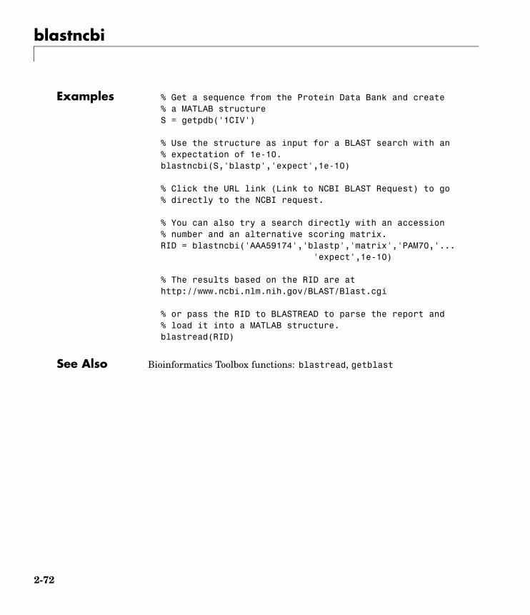
blastncbi
Examples % Get a sequence from the Protein Data Bank and create% a MATLAB structureS = getpdb('1CIV')
% Use the structure as input for a BLAST search with an% expectation of 1e-10.blastncbi(S,'blastp','expect',1e-10)
% Click the URL link (Link to NCBI BLAST Request) to go% directly to the NCBI request.
% You can also try a search directly with an accession% number and an alternative scoring matrix.RID = blastncbi('AAA59174','blastp','matrix','PAM70,'...
'expect',1e-10)
% The results based on the RID are athttp://www.ncbi.nlm.nih.gov/BLAST/Blast.cgi
% or pass the RID to BLASTREAD to parse the report and% load it into a MATLAB structure.blastread(RID)
See Also Bioinformatics Toolbox functions: blastread, getblast
2-72

blastread
Purpose Read data from NCBI BLAST report file
Syntax Data = blastread(File)
Arguments File NCBI BLAST formatted report file. Enter a file name,a path and file name, or a URL pointing to a file. Filecan also be a MATLAB character array that containsthe text for a NCBI BLAST report.
Description BLAST (Basic Local Alignment Search Tool) reports offer a fast andpowerful comparative analysis of interesting protein and nucleotidesequences against known structures in existing online databases.BLAST reports can be lengthy, and parsing the data from the variousformats can be cumbersome.
Data = blastread(File) reads a BLAST report from an NCBIformatted file (File) and returns a data structure (Data) containingfields corresponding to the BLAST keywords. blastread parses thebasic BLAST reports BLASTN, BLASTP, BLASTX, TBLASTN, and TBLASTX.
Data contains the following fields:
Field Description
RID
Algorithm
Query
Database
Hits.Name
Hits.Length
Hits.HSP.Score
Hits.HSP.Expect
2-73
blastread
Field Description
Hits.HSP.Identities
Hits.HSP.Positives
Hits.HSP.Gaps
Hits.HSP.Frame
Hits.HSP.Strand
Hits.HSP.Alignment
Hits.HSPs.QueryIndices
Hits.HSPs.SubjectIndices
Statistics
Examples 1 Create a BLAST request with a GenPept accession number.
RID = blastncbi('AAA59174', 'blastp', 'expect', 1e-10)
2 Pass the RID to getblast, download the report and save the reportto a text file.
getblast(RID, 'ToFile' ,'AAA59174_BLAST.rpt')
3 Using the saved file, read the results into a MATLAB structure.
results = blastread('AAA59174_BLAST.rpt')
References For more information about reading and interpreting BLAST reports,see
http://www.ncbi.nlm.nih.gov/Education/BLASTinfo/Blast_output.html
See Also Bioinformatics Toolbox functions: blastncbi, getblast
2-74
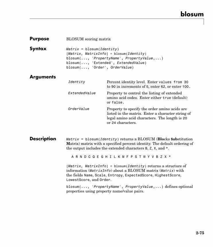
blosum
Purpose BLOSUM scoring matrix
Syntax Matrix = blosum(Identity)[Matrix, MatrixInfo] = blosum(Identity)blosum(..., 'PropertyName', PropertyValue,...)blosum(..., 'Extended', ExtendedValue)blosum(..., 'Order', OrderValue)
ArgumentsIdentity Percent identity level. Enter values from 30
to 90 in increments of 5, enter 62, or enter 100.
ExtendedValue Property to control the listing of extendedamino acid codes. Enter either true (default)or false.
OrderValue Property to specify the order amino acids arelisted in the matrix. Enter a character string oflegal amino acid characters. The length is 20or 24 characters.
Description Matrix = blosum(Identity) returns a BLOSUM (Blocks SubstitutionMatrix) matrix with a specified percent identity. The default ordering ofthe output includes the extended characters B, Z, X, and *.
A R N D C Q E G H I L K M F P S T W Y V B Z X *
[Matrix, MatrixInfo] = blosum(Identity) returns a structure ofinformation (MatrixInfo) about a BLOSUM matrix (Matrix) withthe fields Name, Scale, Entropy, ExpectedScore, HighestScore,LowestScore, and Order.
blosum(..., 'PropertyName', PropertyValue,...) defines optionalproperties using property name/value pairs.
2-75

blosum
blosum(..., 'Extended', ExtendedValue), if Extended is false,returns the scoring matrix for the standard 20 amino acids. Ordering ofthe output when Extended is false is
A R N D C Q E G H I L K M F P S T W Y V
blosum(..., 'Order', OrderValue) returns a BLOSUM matrixordered by an amino acid sequence (OrderString).
Examples Return a BLOSUM matrix with a value of 50.
B50 = blosum(50)
Return a BLOSUM matrix with the amino acids in a specific order.
B75 = blosum(75,'Order','CSTPAGNDEQHRKMILVFYW')
See Also Bioinformatics Toolbox functions dayhoff, gonnet, nwalign, pam,swalign
2-76

celintensityread
Purpose Read probe intensities from Affymetrix CEL files (Windows 32)
Syntax ProbeStructure = celintensityread(CELFiles, CDFFile)ProbeStructure = celintensityread(..., 'CELPath',CELPathValue, ...)ProbeStructure = celintensityread(..., 'CDFPath',
CDFPathValue, ...)ProbeStructure = celintensityread(..., 'PMOnly',PMOnlyValue,
...)ProbeStructure = celintensityread(..., 'Verbose',
VerboseValue, ...)
Arguments CELFiles Cell array of CEL file names. If you set CELFilesto '*', then it reads all CEL files in the currentdirectory. If you set CELFiles to ' ', then itopens the Select CEL Files dialog box from whichyou select the CEL files. From this dialog box, youcan press and hold Ctrl or Shift while clicking toselect multiple CEL files.
CDFFile String specifying a CDF file name. If you setCDFFile to ' ', then it opens the Select CDF Filedialog box from which you select the CDF file.
CELPathValue String specifying the path and directory wherethe files specified in CELFiles are stored.
CDFPathValue String specifying the path and directory wherethe file specified in CDFFile is stored.
2-77
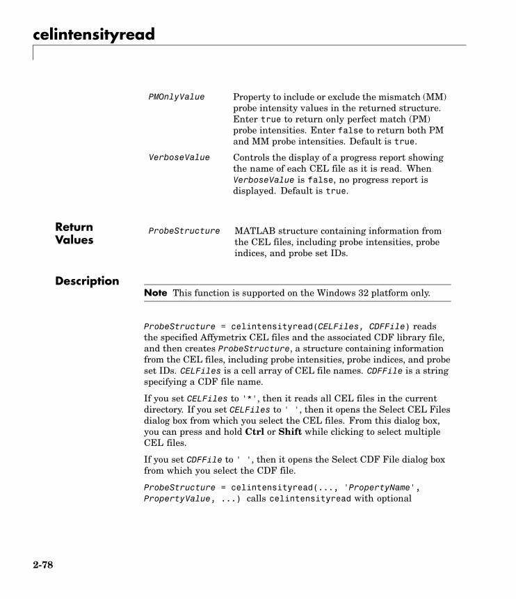
celintensityread
PMOnlyValue Property to include or exclude the mismatch (MM)probe intensity values in the returned structure.Enter true to return only perfect match (PM)probe intensities. Enter false to return both PMand MM probe intensities. Default is true.
VerboseValue Controls the display of a progress report showingthe name of each CEL file as it is read. WhenVerboseValue is false, no progress report isdisplayed. Default is true.
ReturnValues
ProbeStructure MATLAB structure containing information fromthe CEL files, including probe intensities, probeindices, and probe set IDs.
DescriptionNote This function is supported on the Windows 32 platform only.
ProbeStructure = celintensityread(CELFiles, CDFFile) readsthe specified Affymetrix CEL files and the associated CDF library file,and then creates ProbeStructure, a structure containing informationfrom the CEL files, including probe intensities, probe indices, and probeset IDs. CELFiles is a cell array of CEL file names. CDFFile is a stringspecifying a CDF file name.
If you set CELFiles to '*', then it reads all CEL files in the currentdirectory. If you set CELFiles to ' ', then it opens the Select CEL Filesdialog box from which you select the CEL files. From this dialog box,you can press and hold Ctrl or Shift while clicking to select multipleCEL files.
If you set CDFFile to ' ', then it opens the Select CDF File dialog boxfrom which you select the CDF file.
ProbeStructure = celintensityread(..., 'PropertyName',PropertyValue, ...) calls celintensityread with optional
2-78

celintensityread
properties that use property name/property value pairs. You canspecify one or more properties in any order. Each PropertyName mustbe enclosed in single quotation marks and is case insensitive. Theseproperty name/property value pairs are as follows:
ProbeStructure = celintensityread(..., 'CELPath', CELPathValue,...) specifies a path and directory where the files specified in CELFilesare stored.
ProbeStructure = celintensityread(..., 'CDFPath', CDFPathValue,...) specifies a path and directory where the file specified in CDFFile isstored.
ProbeStructure = celintensityread(..., 'PMOnly',PMOnlyValue, ...) includes or excludes the mismatch (MM) probeintensity values. When PMOnlyValue is true, celintensityreadreturns only perfect match (PM) probe intensities. When PMOnlyValueis false, celintensityread returns both PM and MM probeintensities. Default is true.
ProbeStructure contains the following fields.
Field Description
CDFName File name of the Affymetrix library CDF file.
CELNames Cell array of names of the Affymetrix CEL files.
NumProbeSets Number of probe sets in each CEL file.
ProbeSetIDs Cell array of the probe set IDs from the AffymetrixCDF library file.
ProbeIndices Column vector containing probe indexinginformation. Probes within a probe set arenumbered 0 through N - 1, where N is the numberof probes in the probe set.
2-79
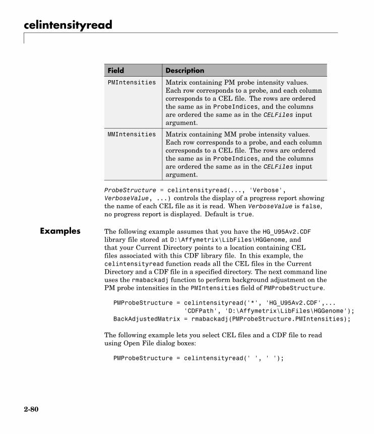
celintensityread
Field Description
PMIntensities Matrix containing PM probe intensity values.Each row corresponds to a probe, and each columncorresponds to a CEL file. The rows are orderedthe same as in ProbeIndices, and the columnsare ordered the same as in the CELFiles inputargument.
MMIntensities Matrix containing MM probe intensity values.Each row corresponds to a probe, and each columncorresponds to a CEL file. The rows are orderedthe same as in ProbeIndices, and the columnsare ordered the same as in the CELFiles inputargument.
ProbeStructure = celintensityread(..., 'Verbose',VerboseValue, ...) controls the display of a progress report showingthe name of each CEL file as it is read. When VerboseValue is false,no progress report is displayed. Default is true.
Examples The following example assumes that you have the HG_U95Av2.CDFlibrary file stored at D:\Affymetrix\LibFiles\HGGenome, andthat your Current Directory points to a location containing CELfiles associated with this CDF library file. In this example, thecelintensityread function reads all the CEL files in the CurrentDirectory and a CDF file in a specified directory. The next command lineuses the rmabackadj function to perform background adjustment on thePM probe intensities in the PMIntensities field of PMProbeStructure.
PMProbeStructure = celintensityread('*', 'HG_U95Av2.CDF',...'CDFPath', 'D:\Affymetrix\LibFiles\HGGenome');
BackAdjustedMatrix = rmabackadj(PMProbeStructure.PMIntensities);
The following example lets you select CEL files and a CDF file to readusing Open File dialog boxes:
PMProbeStructure = celintensityread(' ', ' ');
2-80
celintensityread
See Also Bioinformatics Toolbox functions: affyread, agferead, gprread,probelibraryinfo, probesetlink, probesetlookup, probesetplot,probesetvalues, sptread
2-81

classperf
Purpose Evaluate performance of classifier
Syntax classperfcp = classperf(groundtruth)classperf(cp, classout)classperf(cp, classout, testidx)cp = classperf(groundtruth, classout,...)cp = classperf(..., 'Positive', PositiveValue, 'Negative',
NegativeValue)
Description classperf provides an interface to keep track of the performanceduring the validation of classifiers. classperf creates and updatesa classifier performance object (CP) that accumulates the results ofthe classifier. Later, classification standard performance parameterscan be accessed using the function get or as fields in structures.Some of these performance parameters are ErrorRate, CorrectRate,ErrorDistributionByClass, Sensitivity and Specificity. classperf,without input arguments, displays all the available performanceparameters.
cp = classperf(groundtruth) creates and initializes an empty object.CP is the handle to the object. groundtruth is a vector containing thetrue class labels for every observation. groundtruth can be a numericvector or a cell array of strings. When used in a cross-validation designexperiment, groundtruth should have the same size as the totalnumber of observations.
classperf(cp, classout) updates the CP object with the classifieroutput classout. classout is the same size and type as groundtruth.When classout is numeric and groundtruth is a cell array of strings,the function grp2idx is used to create the index vector that linksclassout to the class labels. When classout is a cell array of strings,an empty string, '', represents an inconclusive result of the classifier.For numeric arrays, NaN represents an inconclusive result.
classperf(cp, classout, testidx) updates the CP object withthe classifier output classout. classout has smaller size thangroundtruth, and testidx is an index vector or a logical index vector of
2-82
classperf
the same size as groundtruth, which indicates the observations thatwere used in the current validation.
cp = classperf(groundtruth, classout,...) creates and updatesthe CP object with the first validation. This form is useful when youwant to know the performance of a single validation.
cp = classperf(..., 'Positive', PositiveValue, 'Negative',NegativeValue) sets the 'positive' and 'negative' labels to identifythe target disorder and the control classes. These labels are used tocompute clinical diagnostic test performance. p and n must consist ofdisjoint sets of the labels used in groundtruth. For example, if
groundtruth = [1 2 2 1 3 4 4 1 3 3 3 2]
you could set
p = [1 2];n = [3 4];
If groundtruth is a cell array of strings, p and n can either be cellarrays of strings or numeric vectors whose entries are subsets ofgrp2idx(groundtruth). PositiveValue defaults to the first classreturned by grp2idx(groundtruth), while NegativeValue defaultsto all the others. In clinical tests, inconclusive values ('' or NaN)are counted as false negatives for the computation of the specificityand as false positives for the computation of the sensitivity, that is,inconclusive results may decrease the diagnostic value of the test.Tested observations for which true class is not within the union ofPositiveValue and NegativeValue are not considered. However,tested observations that result in a class not covered by the vectorgroundtruth are counted as inconclusive.
Examples % Classify the fisheriris data with a K-Nearest Neighbor
classifier load fisheriris
c = knnclassify(meas,meas,species,4,'euclidean','Consensus');
cp = classperf(species,c)
get(cp)
2-83

classperf
% 10-fold cross-validation on the fisheriris data using linear
% discriminant analysis and the third column as only feature for
% classification
load fisheriris
indices = crossvalind('Kfold',species,10);
cp = classperf(species); % initializes the CP object
for i = 1:10
test = (indices == i); train = ~test;
class = classify(meas(test,3),meas(train,3),species(train));
% updates the CP object with the current classification results
classperf(cp,class,test)
end
cp.CorrectRate % queries for the correct classification rate
cp =
biolearning.classperformance
Label: ''
Description: ''
ClassLabels: {3x1 cell}
GroundTruth: [150x1 double]
NumberOfObservations: 150
ControlClasses: [2x1 double]
TargetClasses: 1
ValidationCounter: 1
SampleDistribution: [150x1 double]
ErrorDistribution: [150x1 double]
SampleDistributionByClass: [3x1 double]
ErrorDistributionByClass: [3x1 double]
CountingMatrix: [4x3 double]
CorrectRate: 1
ErrorRate: 0
InconclusiveRate: 0.0733
ClassifiedRate: 0.9267
Sensitivity: 1
2-84
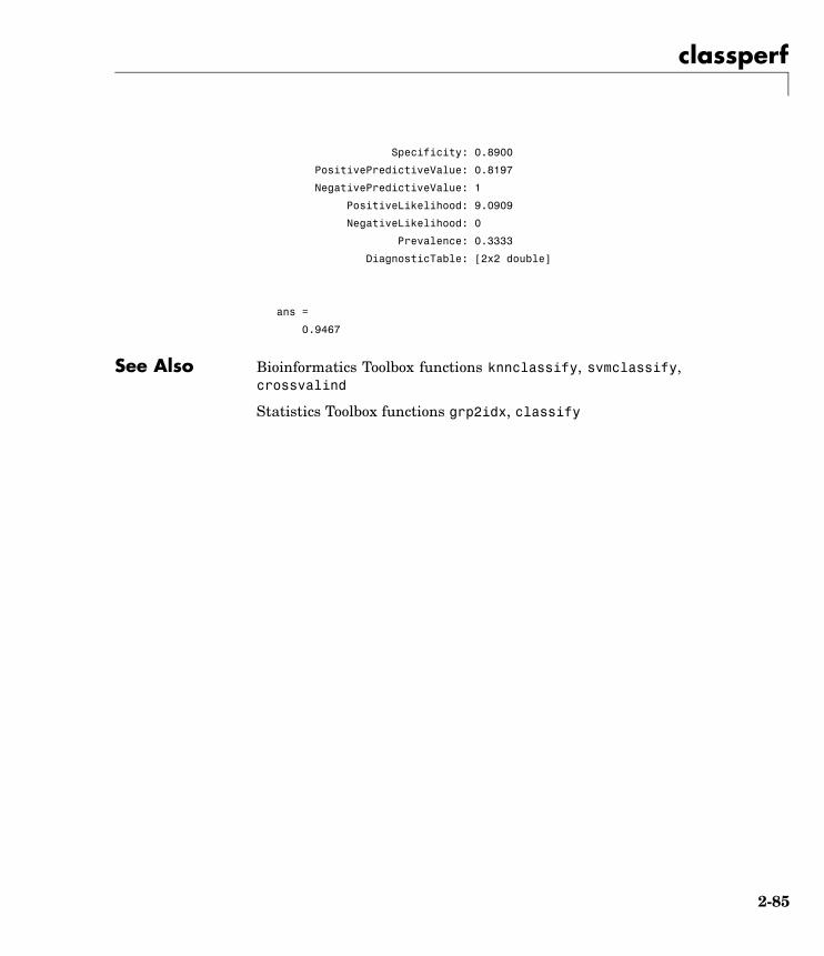
classperf
Specificity: 0.8900
PositivePredictiveValue: 0.8197
NegativePredictiveValue: 1
PositiveLikelihood: 9.0909
NegativeLikelihood: 0
Prevalence: 0.3333
DiagnosticTable: [2x2 double]
ans =
0.9467
See Also Bioinformatics Toolbox functions knnclassify, svmclassify,crossvalind
Statistics Toolbox functions grp2idx, classify
2-85

cleave
Purpose Cleave amino acid sequence with enzyme
Syntax Fragments = cleave(SeqAA, PeptidePattern, Position)[Fragments, CuttingSites] = cleave(...)[Fragments, CuttingSites, Lengths] = cleave(...)cleave(..., 'PropertyName', PropertyValue,...)cleave(..., 'PartialDigest', PartialDigestValue)
Arguments SeqAA Amino acid sequence. Enter a characterstring or a vector of integers from the table .
Examples: 'ARN' or [1 2 3]. You can alsoenter a structure with the field Sequence.
PeptidePattern Short amino acid sequence to search in alarger sequence. Enter a character string,vector of integers, or a regular expression.
Position Position on the PeptidePattern wherethe sequence is cleaved. Enter a positionwithin the PeptidePattern. Position 0corresponds to the N terminal end of thePepetidePattern.
PartialDigestValue Property to specify the probability that acleavage site will be cleaved. Enter a valuefrom 0 to 1 (default).
Description Fragments = cleave(SeqAA, PeptidePattern, Position) cuts anamino acid sequence (SeqAA) into parts at the specified cleavage sitespecified by a peptide pattern and position.
[Fragments, CuttingSites] = cleave(...) returns a numericvector with the indices representing the cleave sites. A 0 (zero) is addedto the list, so numel(Fragments)==numel(CuttingSites). You can useCuttingSites + 1 to point to the first amino acid of every fragmentrespective to the original sequence.
2-86

cleave
[Fragments, CuttingSites, Lengths] = cleave(...) returns anumeric vector with the lengths of every fragment.
cleave(..., 'PropertyName', PropertyValue,...) defines optionalproperties using property name/value pairs.
cleave(..., 'PartialDigest', PartialDigestValue) simulates apartial digestion where PartialDigest is the probability of a cleavagesite being cut.
The following table lists some common proteases and their cleavagesites.
Protease Peptide Pattern Position
Trypsin [KR](?!P) 1
Chymotrypsin [WYF](?!P) 1
Glutamine C [ED](?!P) 1
Lysine C [K](?!P) 1
Aspartic acid N D 1
Examples 1 Get a protein sequence from the GenPept database.
S = getgenpept('AAA59174')
2 Cleave the sequence using trypsin. Trypsin cleaves after K or R whenthe next residue is not P.
[parts, sites, lengths] = cleave(S.Sequence,'[KR](?!P)',1);for i=1:10
fprintf('%5d%5d %s\n',sites(i),lengths(i),parts{i})end
0 6 MGTGGR6 1 R7 34 GAAAAPLLVAVAALLLGAAGHLYPGEVCPGMDIR
41 5 NNLTR
2-87

cleave
46 21 LHELENCSVIEGHLQILLMFK67 7 TRPEDFR74 6 DLSFPK80 12 LIMITDYLLLFR92 8 VYGLESLK
100 10 DLFPNLTVIR
See Also Bioinformatics Toolbox functions: rebasecuts, restrict,seqshowwords
MATLAB function: regexp
2-88
clustergram
Purpose Create dendrogram and heat map
Syntax clustergram(Data)clustergram(Data, ...'RowLabels', RowLabelsValue, ...)clustergram(Data, ...'ColumnLabels',ColumnLabelsValue, ...)clustergram(Data, ...'Pdist', PdistValue, ...)clustergram(Data, ...'Linkage', LinkageValue, ...)clustergram(Data, ...'Dendrogram', DendrogramValue, ...)clustergram(Data, ...'OptimalLeafOrder',
OptimalLeafOrderValue, ...)clustergram(Data, ...'ColorMap', ColorMapValue, ...)clustergram(Data, ...'SymmetricRange', SymmetricRangeValue,
...)clustergram(Data, ...'Dimension', DimensionValue, ...)clustergram(Data, ...'Ratio', RatioValue, ...)
ArgumentsData Matrix in which each row corresponds to
a gene and each column corresponds to asingle experiment or microarray.
RowLabelsValue Vector of numbers or cell array of textstrings to label the rows in Data.
ColumnLabelsValue Vector of numbers or cell array of textstrings to label the columns in Data.
2-89

clustergram
PdistValue String to specify the distance metric to passto the pdist function (Statistics Toolbox)to use to calculate the pair-wise distancesbetween observations. For information onchoices, see the pdist function. Default iseuclidean.
Note If the distance metric requires extraarguments, then PdistValue is a cellarray. For example, to use the Minkowskidistance with exponent P, you would use{'minkowski', P}.
LinkageValue String to specify the linkage method topass to the linkage function (StatisticsToolbox) to use to create the hierarchicalcluster tree. For information on choices, seethe linkage function. Default is average.
DendrogramValue Cell array of property name/propertyvalue pairs to pass to the dendrogramfunction (Statistics Toolbox) to create thedendrogram plot. For information onchoices, see the dendrogram function.
2-90

clustergram
OptimalLeafOrderValue Property to enable or disable the optimalleaf ordering calculation, which determinesthe leaf order that maximizes the similaritybetween neighboring leaves. Choices aretrue (enable) or false (disable). Defaultdepends on the size of Data. If the numberof rows or columns in Data is greater than1000, default is false; otherwise, defaultis true.
Note Disabling the optimal leaf orderingcalculation can be useful when workingwith large data sets because thiscalculation uses a large amount of memoryand can be very time consuming.
ColorMapValue Either of the following:• M-by-3 matrix of RGB values
• Name or function handle of a functionthat returns a color map
Default is redgreencmap.
SymmetricRangeValue Property to force the color range of the heatmap to be symmetric around zero. Choicesare true (default) or false.
2-91
clustergram
DimensionValue Property to specify either aone-dimensional or two-dimensionalclustergram. Choices are 1 (default) or 2.
RatioValue Either of the following:• Scalar
• Two-element vector
Default is 1/5.
Description clustergram(Data) creates a dendrogram and heat map from the geneexpression data in the matrix Data. It uses hierarchical clusteringwith euclidean distance metric and average linkage to generate thehierarchical tree. The clustering is performed on the rows in matrixData, in which the rows correspond to genes and the columns correspondto different microarrays. To cluster the columns instead of the rows,transpose the data using the transpose (') operator.
clustergram(Data, ...'PropertyName', PropertyValue, ...)calls clustergram with optional properties that use propertyname/property value pairs. You can specify one or more properties inany order. Each PropertyName must be enclosed in single quotationmarks and is case insensitive. These property name/property valuepairs are as follows:
clustergram(Data, ...'RowLabels', RowLabelsValue, ...) usesthe contents of RowLabelsValue, a vector of numbers or cell array oftext strings, as labels for the rows in Data.
clustergram(Data, ...'ColumnLabels', ColumnLabelsValue,...) uses the contents of ColumnLabelsValue, a vector of numbers orcell array of text strings, as labels for the columns in Data.
clustergram(Data, ...'Pdist', PdistValue, ...) specifies thedistance metric to pass to the pdist function (Statistics Toolbox) to useto calculate the pair-wise distances between observations. PdistValueis a string. For information on choices, see the pdist function. Defaultis euclidean.
2-92

clustergram
Note If the distance metric requires extra arguments, then PdistValueis a cell array. For example, to use the Minkowski distance withexponent P, you would use {'minkowski', P}.
clustergram(Data, ...'Linkage', LinkageValue, ...) specifiesthe linkage method to pass to the linkage function (Statistics Toolbox)to use to create the hierarchical cluster tree. LinkageValue is astring. For information on choices, see the linkage function. Defaultis average.
clustergram(Data, ...'Dendrogram', DendrogramValue,...) specifies property name/property value pairs to pass to thedendrogram function (Statistics Toolbox) to create the dendrogram plot.DendrogramValue is a cell array of property name/property value pairs.For information on choices, see the dendrogram function.
clustergram(Data, ...'OptimalLeafOrder',OptimalLeafOrderValue, ...) enables or disables the optimal leafordering calculation, which determines the leaf order that maximizesthe similarity between neighboring leaves. Choices are true (enable) orfalse (disable). Default depends on the size of Data. If the numberof rows or columns in Data is greater than 1000, default is false;otherwise, default is true.
Note Disabling the optimal leaf ordering calculation can be usefulwhen working with large data sets because this calculation uses a largeamount of memory and can be very time consuming.
clustergram(Data, ...'ColorMap', ColorMapValue, ...) specifiesthe color map to use to create the clustergram. This controls the colorsused to display the heat map. ColorMapValue is either a M-by-3 matrixof RGB values or the name or function handle of a function that returnsa color map. Default is redgreencmap.
2-93
clustergram
clustergram(Data, ...'SymmetricRange', SymmetricRangeValue,...), controls whether the color range of the heat map is symmetricaround zero. SymmetricRangeValue can be true (default) or false.
clustergram(Data, ...'Dimension', DimensionValue, ...)specifies whether to create a one-dimensional or two-dimensionalclustergram. Choices are 1 (default) or 2. The one-dimensionalclustergram clusters the rows of the data. The two-dimensionalclustergram creates the one-dimensional clustergram, and then clustersthe columns of the row-clustered data.
clustergram(Data, ...'Ratio', RatioValue, ...) specifies theratio of the space that the dendrogram(s) use in the X and Y directions,relative to the size of the heat map. If RatioValue is a scalar, it is usedas the ratio for both directions. If RatioValue is a two-element vector,the first element is used for the X ratio, and the second element is usedfor the Y ratio. The Y ratio is ignored for one-dimensional clustergrams.Default ratio is 1/5.
Tip Click and hold the mouse button on the heat map to display theintensity value, column label, and row label for that area of the heatmap. View row labels by using the zoom icon to zoom the right sideof the clustergram.
Examples The following example uses data from an experiment (DeRisi et al.,1997) that used DNA microarrays to study temporal gene expression ofalmost all genes in Saccharomyces cerevisiae during the metabolic shiftfrom fermentation to respiration. Expression levels were measured atseven time points during the diauxic shift.
1 Load the filtered yeast data provided with Bioinformatics Toolbox,and then create a clustergram from the gene expression data in theyeastvalues matrix.
load filteredyeastdataclustergram(yeastvalues)
2-94
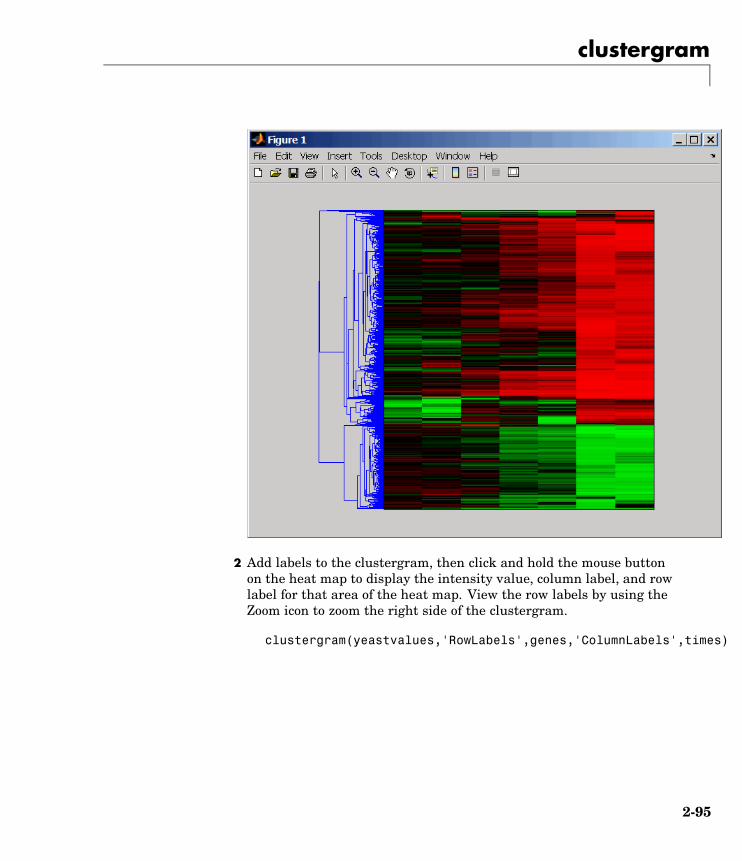
clustergram
2 Add labels to the clustergram, then click and hold the mouse buttonon the heat map to display the intensity value, column label, and rowlabel for that area of the heat map. View the row labels by using theZoom icon to zoom the right side of the clustergram.
clustergram(yeastvalues,'RowLabels',genes,'ColumnLabels',times)
2-95
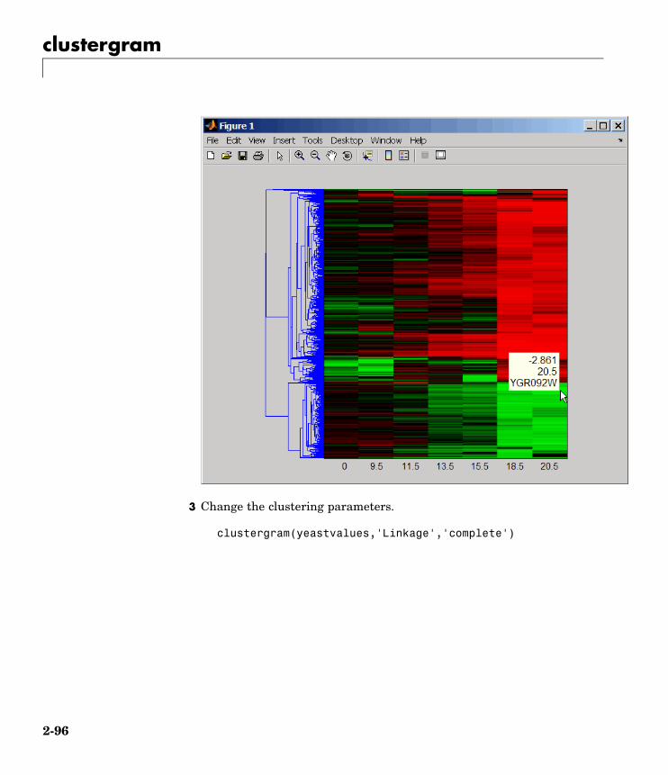
clustergram
3 Change the clustering parameters.
clustergram(yeastvalues,'Linkage','complete')
2-96

clustergram
4 Change the color of the groups of nodes in the dendrogram whoselinkage is less than a threshold of 5.
clustergram(yeastvalues,'RowLabels',genes,...'Dendrogram',{'colorthreshold',5})
2-97

clustergram
References [1] Bar-Joseph, Z., Gifford, D.K., and Jaakkola, T.S. (2001). Fast optimalleaf ordering for hierarchical clustering. Bioinformatics 17, Suppl 1:S22– 9. PMID: 11472989.
[2] Eisen, M.B., Spellman, P.T., Brown, P.O., and Botstein, D. (1998).Cluster analysis and display of genome-wide expression patterns. ProcNatl Acad Sci USA 95, 14863 – 8.
2-98

clustergram
[3] DeRisi, J.L., Iyer, V.R., and Brown, P.O. (1997) Exploring themetabolic and genetic control of gene expression on a genomic scale.Science 278, 680–686s.
See Also Bioinformatics Toolbox function: redgreencmap
Statistics Toolbox functions: cluster, dendrogram, linkage, pdist
2-99

codonbias
Purpose Calculate codon frequency for each amino acid in DNA sequence
Syntax codonbias(SeqDNA)codonbias(..., 'PropertyName', PropertyValue,...)codonbias(..., 'GeneticCode', GeneticCodeValue)codonbias(..., 'Frame', FrameValue)codonbias(..., 'Reverse', ReverseValue)codonbias(..., 'Pie', PieValue)
ArgumentsSeqDNA Nucleotide sequence (DNA or RNA). Enter a character
string with the letters A, T or U, C, and G or a vectorof integers. You can also enter a structure with thefield Sequence. codonbias does not count ambiguousbases or gaps.
Description Many amino acids are coded by two or more nucleic acid codons.However, the probability that a codon (from the various possible codonsfor an amino acid) is used to code an amino acid is different betweensequences. Knowing the frequency of each codon in a protein codingsequence for each amino acid is a useful statistic.
codonbias(SeqDNA) calculates the codon frequency in percent for eachamino acid in a DNA sequence (SeqDNA).
codonbias(..., 'PropertyName', PropertyValue,...) definesoptional properties using property name/value pairs.
codonbias(..., 'GeneticCode', GeneticCodeValue) selects analternative genetic code (GenetidCodeValue). The default value is'Standard' or 1. For a list of genetic codes, see .
codonbias(..., 'Frame', FrameValue) selects a reading frame(FrameValue). FrameValue can be 1 (default), 2, or 3.
codonbias(..., 'Reverse', ReverseValue), when ReverseValue istrue, returns the codon frequency for the reverse complement of theDNA sequence (SeqDNA).
2-100

codonbias
codonbias(..., 'Pie', PieValue), when PieValue is true, createsa figure of 20 pie charts for each amino acid.
Example 1 Import a nucleotide sequence from GenBank to MATLAB. Forexample, get the DNA sequence that codes for a human insulinreceptor.
S = getgenbank('M10051');
2 Calculate the codon frequency for each amino acid and plot theresults.
cb = codonbias(S.Sequence,'PIE',true)
cb.Alaans =
Codon: {'GCA' "GCC' "GCG' 'GCT'}Freq: [0.1600 0.3867 0.2533 02000]
MATLAB draws a figure with 20 pie charts for the 20 amino acids.
2-101
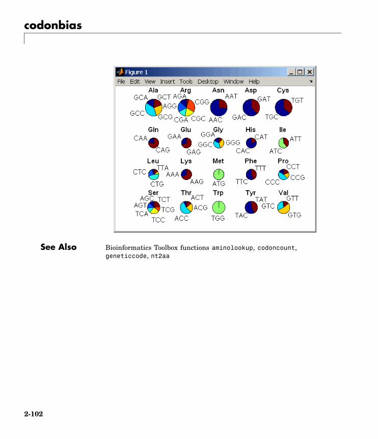
codonbias
See Also Bioinformatics Toolbox functions aminolookup, codoncount,geneticcode, nt2aa
2-102
codoncount
Purpose Count codons in nucleotide sequence
Syntax Codons = codoncount(SeqNT)codoncount(..., 'PropertyName', PropertyValue,...)codoncount(..., 'Frame', FrameValue)codoncount(..., 'Reverse', ReverseValue)codoncount(..., 'Figure', FigureValue)
Arguments SeqNT Nucleotide sequence. Enter a character string orvector of integers. You can also enter a structurewith the field Sequence.
FrameValue Property to select a reading frame. Enter 1 (default),2, or 3.
ReverseValue Property to control returning the complementsequence. Enter true or false (default).
FigureValue Property to control plotting a heat map. Entereither true or false (default).
Description Codons = codoncount(SeqNT) counts the number of codon in asequence (SeqNT) and returns the codon counts in a structure with thefields AAA, AAC, AAG, ..., TTG, TTT.
• For sequences that have codons with the character U, the U charactersare added to codons with T characters.
• If the sequence contains ambiguous nucleotide characters (R Y K MS W B D H V N) , or gaps indicated with a hyphen (-), this functioncreates a field Others and displays a warning message.
Warning: Ambiguous symbols 'symbol' appearin the sequence.These will be in Others.
2-103

codoncount
• If the sequence contains undefined nucleotide characters (E F H IJ L O P Q X Z), codoncount ignores the characters and displays awarning message.
Warning: Unknown symbols 'symbol' appearin the sequence.These will be ignored.
[Codons, CodonArray] = codoncount(SeqNT) returns a 4x4x4 array(CodonArray) with the raw count data for each codon. The threedimensions correspond to the three positions in the codon. For example,the element (2,3,4) of the array gives the number of CGT codons whereA <=> 1, C <=> 2, G <=> 3, and T <=> 4.
codoncount(..., 'PropertyName', PropertyValue,...) definesoptional properties using property name/value pairs.
codoncount(..., 'Frame', FrameValue) counts the codons in aspecific reading frame.
codoncount(..., 'Reverse', ReverseValue), when ReverseValue istrue, counts the codons for the reverse complement of the sequence.
codoncount(..., 'Figure', FigureValue), when FigureValue istrue displays a figure showing a heat map of the codon counts.
Examples Count the number of standard codons in a nucleotide sequence.
codons = codoncount('AAACGTTA')
codons =AAA: 1 ATC: 0 CGG: 0 GCT: 0 TCA: 0AAC: 0 ATG: 0 CGT: 1 GGA: 0 TCC: 0AAG: 0 ATT: 0 CTA: 0 GGC: 0 TCG: 0AAT: 0 CAA: 0 CTC: 0 GGG: 0 TCT: 0ACA: 0 CAC: 0 CTG: 0 GGT: 0 TGA: 0ACC: 0 CAG: 0 CTT: 0 GTA: 0 TGC: 0ACG: 0 CAT: 0 GAA: 0 GTC: 0 TGG: 0ACT: 0 CCA: 0 GAC: 0 GTG: 0 TGT: 0
2-104

codoncount
AGA: 0 CCC: 0 GAG: 0 GTT: 0 TTA: 0AGC: 0 CCG: 0 GAT: 0 TAA: 0 TTC: 0AGG: 0 CCT: 0 GCA: 0 TAC: 0 TTG: 0AGT: 0 CGA: 0 GCC: 0 TAG: 0 TTT: 0ATA: 0 CGC: 0 GCG: 0 TAT: 0
Count the codons in the second frame for the reverse complement ofa sequence.
r2codons = codoncount('AAACGTTA', 'Frame',2,...'Reverse',true);
Create a heat map for the codons in a nucleotide sequence.
a = randseq(1000);codoncount(a,'Figure', true);
2-105

codoncount
See Also Bioinformatics Toolbox functions aacount , basecount, baselookup,codonbias, dimercount, nmercount, ntdensity, seqrcomplement,seqwordcount
2-106

cpgisland
Purpose Locate CpG islands in DNA sequence
Syntax cpgisland(SeqDNA)cpgisland(..., 'PropertyName', PropertyValue,...)cpgisland(..., 'Window', WindowValue)cpgisland(..., 'MinIsland', MinIslandValue)cpgisland(..., 'CpGoe', CpGoeValue)cpgisland(..., 'GCmin', GCminValue)cpgisland(..., 'Plot', PlotValue)
ArgumentsSeqDNA DNA nucleotide sequence. Enter a character
string with the letters A, T, C, and G. You canalso enter a structure with the field Sequence.cpgisland does not count ambiguous bases orgaps.
Description cpgisland(SeqDNA) finds CpG islands by marking bases within amoving window of 100 DNA bases with a GC content greater than 50%and a CpGobserved/CpGexpected ratio greater than 60%.
cpgisland(..., 'PropertyName', PropertyValue,...) definesoptional properties using property name/value pairs.
cpgisland(..., 'Window', WindowValue) specifies the window sizefor calculating GC percent and CpGobserved/CpGexpected ratios fora sequence. The default value is 100 bases. A smaller window sizeincreases the noise in a plot.
cpgisland(..., 'MinIsland', MinIslandValue) specifies theminimum number of consecutive marked bases to report. The defaultvalue is 200 bases.
cpgisland(..., 'CpGoe', CpGoeValue) specifies the minimumCpGobserved/CpGexpected ratio in each window needed to mark abase. Enter a value between 0 and 1. The default value is 0.6. Thisratio is defined as
2-107

cpgisland
CPGobs/CpGexp = (NumCpGs*Length)/(NumGs*NumCs)
cpgisland(..., 'GCmin', GCminValue) specifies the minimum GCpercent in a window needed to mark a base. Enter a value between 0and 1. The default value is 0.5.
cpgisland(..., 'Plot', PlotValue), when Plot is true, plots GCcontent, CpGoe content, CpG islands greater than the minimum islandsize, and all potential CpG islands for the specified criteria.
Example 1 Import a nucleotide sequence from GenBank. For example, get asequence from Homo Sapiens chromosome 12.
S = getgenbank('AC156455');
2 Calculate the CpG islands in the sequence and plot the results.
cpgisland(S.Sequence,'PLOT',true)
MATLAB lists the CpG islands greater than 200 bases and draws afigure.
ans =Starts: [4470 28753 29347 36229]Stops: [5555 29064 29676 36450]
2-108
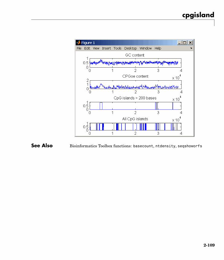
cpgisland
See Also Bioinformatics Toolbox functions: basecount, ntdensity, seqshoworfs
2-109

crossvalind
Purpose Generate cross-validation indices
Syntax Indices = crossvalind('Kfold', N, K)[Train, Test] = crossvalind('HoldOut', N, P)[Train, Test] = crossvalind('LeaveMOut', N, M)[Train, Test] = crossvalind('Resubstitution', N, [P,Q])[...] = crossvalind(Method, Group, ...)[...] = crossvalind(Method, Group, ..., 'Classes', C)[...] = crossvalind(Method, Group, ..., 'Min', MinValue)
Description Indices = crossvalind('Kfold', N, K) returns randomly generatedindices for a K-fold cross-validation of N observations. Indices containsequal (or approximately equal) proportions of the integers 1 throughK that define a partition of the N observations into K disjoint subsets.Repeated calls return different randomly generated partitions. Kdefaults to 5 when omitted. In K-fold cross-validation, K-1 folds areused for training and the last fold is used for evaluation. This process isrepeated K times, leaving one different fold for evaluation each time.
[Train, Test] = crossvalind('HoldOut', N, P) returns logicalindex vectors for cross-validation of N observations by randomlyselecting P*N (approximately) observations to hold out for the evaluationset. P must be a scalar between 0 and 1. P defaults to 0.5 when omitted,corresponding to holding 50% out. Using holdout cross-validation withina loop is similar to K-fold cross-validation one time outside the loop,except that non-disjointed subsets are assigned to each evaluation.
[Train, Test] = crossvalind('LeaveMOut', N, M), where M isan integer, returns logical index vectors for cross-validation of Nobservations by randomly selecting M of the observations to hold out forthe evaluation set. M defaults to 1 when omitted. Using LeaveMOutcross-validation within a loop does not guarantee disjointed evaluationsets. Use K-fold instead.
[Train, Test] = crossvalind('Resubstitution', N, [P,Q])returns logical index vectors of indices for cross-validation of Nobservations by randomly selecting P*N observations for the evaluationset and Q*N observations for training. Sets are selected in order to
2-110
crossvalind
minimize the number of observations that are used in both sets. Pand Q are scalars between 0 and 1. Q=1-P corresponds to holdingout (100*P)%, while P=Q=1 corresponds to full resubstitution. [P,Q]defaults to [1,1] when omitted.
[...] = crossvalind(Method, Group, ...) takes the groupstructure of the data into account. Group is a grouping vector thatdefines the class for each observation. Group can be a numeric vector,a string array, or a cell array of strings. The partition of the groupsdepends on the type of cross-validation: For K-fold, each group isdivided into K subsets, approximately equal in size. For all others,approximately equal numbers of observations from each group areselected for the evaluation set. In both cases the training set contains atleast one observation from each group.
[...] = crossvalind(Method, Group, ..., 'Classes', C)restricts the observations to only those values specified in C. C can be anumeric vector, a string array, or a cell array of strings, but it is of thesame form as Group. If one output argument is specified, it contains thevalue 0 for observations belonging to excluded classes. If two outputarguments are specified, both will contain the logical value false forobservations belonging to excluded classes.
[...] = crossvalind(Method, Group, ..., 'Min', MinValue)sets the minimum number of observations that each group has in thetraining set. Min defaults to 1. Setting a large value for Min can help tobalance the training groups, but adds partial resubstitution when thereare not enough observations. You cannot set Min when using K-foldcross-validation.
Examples Create a 10-fold cross-validation to compute classification error.
load fisheririsindices = crossvalind('Kfold',species,10);cp = classperf(species);for i = 1:10
test = (indices == i); train = ~test;class = classify(meas(test,:),meas(train,:),species(train,:));
2-111

crossvalind
classperf(cp,class,test)endcp.ErrorRate
Approximate a leave-one-out prediction error estimate.
load carbigx = Displacement; y = Acceleration;N = length(x);sse = 0;for i = 1:100
[train,test] = crossvalind('LeaveMOut',N,1);yhat = polyval(polyfit(x(train),y(train),2),x(test));sse = sse + sum((yhat - y(test)).^2);
endCVerr = sse / 100
Divide cancer data 60/40 without using the 'Benign' observations.Assume groups are the true labels of the observations.
labels = {'Cancer','Benign','Control'};groups = labels(ceil(rand(100,1)*3));[train,test] = crossvalind('holdout',groups,0.6,'classes',...
{'Control','Cancer'});sum(test) % Total groups allocated for testingsum(train) % Total groups allocated for training
See Also Bioinformatics Toolbox functions: classperf, knnclassify,svmclassify
Statistics Toolbox functions: classify, grp2idx
2-112

dayhoff
Purpose Dayhoff scoring matrix
Syntax ScoringMatrix = dayhoff
Description ScoringMatrix = dayhoff returns a PAM250 type scoring matrix. Theorder of amino acids in the matrix is A R N D C Q E G H I L K MF P S T W Y V B Z X *.
See Also Bioinformatics Toolbox functions: blosum, gonnet, pam
2-113
dimercount
Purpose Count dimers in sequence
Syntax Dimers = dimercount(SeqNT)[Dimers, Percent] = dimercount(SeqNT)dimercount(..., 'PropertyName', PropertyValue,...)dimercount(..., 'Chart', ChartStyle)
ArgumentsSeqNT Nucleotide sequence. Enter a character string
or vector of integers.
Examples: 'ACGT' and [1 2 3 4].You canalso enter a structure with the fieldSequence.
ChartStyleValue Property to select the type of plot. Enter 'pie'or 'bar'.
Description Dimers = dimercount(SeqNT) counts the number of nucleotide dimersin a 1-by-1 sequence and returns the dimer counts in a structure withthe fields AA, AC, AG, AT, CA, CC, CG, CT, GA, GC, GG, GT, TA, TC, TG, TT.
• For sequences that have dimers with the character U, the U charactersare added to dimers with T characters.
• If the sequence contains ambiguous nucleotide characters (R Y K MS W B D H V N) , or gaps indicated with a hyphen (-), this functioncreates a field Others and displays a warning message.
Warning: Ambiguous symbols 'symbol list' appearin the sequence.These will be in Others.
• If the sequence contains undefined nucleotide characters (E F H IJ L O P Q X Z), codoncount ignores the characters and displays awarning message.
2-114
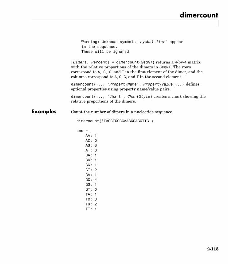
dimercount
Warning: Unknown symbols 'symbol list' appearin the sequence.These will be ignored.
[Dimers, Percent] = dimercount(SeqNT) returns a 4-by-4 matrixwith the relative proportions of the dimers in SeqNT. The rowscorrespond to A, C, G, and T in the first element of the dimer, and thecolumns correspond to A, C, G, and T in the second element.
dimercount(..., 'PropertyName', PropertyValue,...) definesoptional properties using property name/value pairs.
dimercount(..., 'Chart', ChartStyle) creates a chart showing therelative proportions of the dimers.
Examples Count the number of dimers in a nucleotide sequence.
dimercount('TAGCTGGCCAAGCGAGCTTG')
ans =AA: 1AC: 0AG: 3AT: 0CA: 1CC: 1CG: 1CT: 2GA: 1GC: 4GG: 1GT: 0TA: 1TC: 0TG: 2TT: 1
2-115
dimercount
See Also Bioinformatics Toolbox functions aacount, basecount, baselookup,codoncount, nmercount, ntdensity
2-116
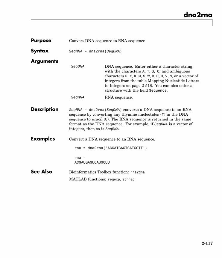
dna2rna
Purpose Convert DNA sequence to RNA sequence
Syntax SeqRNA = dna2rna(SeqDNA)
ArgumentsSeqDNA DNA sequence. Enter either a character string
with the characters A, T, G, C, and ambiguouscharacters R, Y, K, M, S, W, B, D, H, V, N, or a vector ofintegers from the table Mapping Nucleotide Lettersto Integers on page 2-518. You can also enter astructure with the field Sequence.
SeqRNA RNA sequence.
Description SeqRNA = dna2rna(SeqDNA) converts a DNA sequence to an RNAsequence by converting any thymine nucleotides (T) in the DNAsequence to uracil (U). The RNA sequence is returned in the sameformat as the DNA sequence. For example, if SeqDNA is a vector ofintegers, then so is SeqRNA.
Examples Convert a DNA sequence to an RNA sequence.
rna = dna2rna('ACGATGAGTCATGCTT')
rna =ACGAUGAGUCAUGCUU
See Also Bioinformatics Toolbox function: rna2dna
MATLAB functions: regexp, strrep
2-117

dnds
Purpose Estimate synonymous and nonsynonymous substitution rates
Syntax [Dn, Ds, Vardn, Vards] = dnds(SeqNT1, SeqNT2)[Dn, Ds, Vardn, Vards] = dnds(SeqNT1, SeqNT2,...'GeneticCode', GeneticCodeValue, ...)[Dn, Ds, Vardn, Vards] = dnds(SeqNT1, SeqNT2, ...'Method',
MethodValue, ...)[Dn, Ds, Vardn, Vards] = dnds(SeqNT1, SeqNT2, ...'Window',
WindowValue, ...)[Dn, Ds, Vardn, Vards] = dnds(SeqNT1, SeqNT2, ...'Verbose',
VerboseValue, ...)
Arguments SeqNT1, SeqNT2 Nucleotide sequences. Enter either a stringor a structure with the field Sequence.
GeneticCodeValue Property to specify a genetic code. Enter aCode Number or a string with a Code Namefrom the table . If you use a Code Name, youcan truncate it to the first two characters.Default is 1 or Standard.
2-118
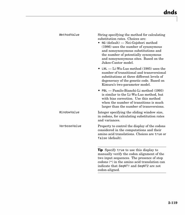
dnds
MethodValue String specifying the method for calculatingsubstitution rates. Choices are:• NG (default) — Nei-Gojobori method
(1986) uses the number of synonymousand nonsynonymous substitutions andthe number of potentially synonymousand nonsynonymous sites. Based on theJukes-Cantor model.
• LWL — Li-Wu-Luo method (1985) uses thenumber of transitional and transversionalsubstitutions at three different levels ofdegeneracy of the genetic code. Based onKimura’s two-parameter model.
• PBL — Pamilo-Bianchi-Li method (1993)is similar to the Li-Wu-Luo method, butwith bias correction. Use this methodwhen the number of transitions is muchlarger than the number of transversions.
WindowValue Integer specifying the sliding window size,in codons, for calculating substitution ratesand variances.
VerboseValue Property to control the display of the codonsconsidered in the computations and theiramino acid translations. Choices are true orfalse (default).
Tip Specify true to use this display tomanually verify the codon alignment of thetwo input sequences. The presence of stopcodons (*) in the amino acid translation canindicate that SeqNT1 and SeqNT2 are notcodon-aligned.
2-119

dnds
ReturnValues
Dn Nonsynonymous substitution rate(s).
Ds Synonymous substitution rate(s).
Vardn Variance for the nonsynonymous substitutionrate(s).
Vards Variance for the synonymous substitutionsrate(s).
Description [Dn, Ds, Vardn, Vards] = dnds(SeqNT1, SeqNT2) estimates thesynonymous and nonsynonymous substitution rates per site betweenthe two homologous nucleotide sequences, SeqNT1 and SeqNT2, bycomparing codons using the Nei-Gojobori method.
dnds returns:
• Dn — Nonsynonymous substitution rate(s).
• Ds — Synonymous substitution rate(s).
• Vardn — Variance for the nonsynonymous substitution rate(s).
• Vards — Variance for the synonymous substitutions rate(s)
This analysis:
• Assumes that the nucleotide sequences, SeqNT1 and SeqNT2, arecodon-aligned, that is, do not have frame shifts.
Tip If your sequences are not codon-aligned, use the nt2aa functionto convert them to amino acid sequences, use the nwalign functionto globally align them, then use the seqinsertgaps function torecover the corresponding codon-aligned nucleotide sequences. SeeEstimating Synonymous and Nonsynonymous Substitution RatesBetween Two Nucleotide Sequences That Are Not Codon-Alignedon page 2-123.
2-120

dnds
• Excludes codons that include ambiguous nucleotide characters orgaps
• Considers the number of codons in the shorter of the two nucleotidesequences
Caution
If SeqNT1 and SeqNT2 are too short or too divergent, saturation can bereached, and dnds returns NaNs and a warning message.
[Dn, Ds, Vardn, Vards] = dnds(SeqNT1, SeqNT2,...'PropertyName', PropertyValue, ...) calls dnds with optionalproperties that use property name/property value pairs. You canspecify one or more properties in any order. Each PropertyName mustbe enclosed in single quotation marks and is case insensitive. Theseproperty name/property value pairs are as follows:
[Dn, Ds, Vardn, Vards] = dnds(SeqNT1, SeqNT2,...'GeneticCode', GeneticCodeValue, ...) calculates synonymousand nonsynonymous substitution rates using the specified genetic code.Enter a Code Number or a string with a Code Name from the table. Ifyou use a Code Name, you can truncate it to the first two characters.Default is 1 or Standard.
[Dn, Ds, Vardn, Vards] = dnds(SeqNT1, SeqNT2, ...'Method',MethodValue, ...) allows you to calculate synonymous andnonsynonymous substitution rates using the following algorithms:
• NG (default) — Nei-Gojobori method (1986) uses the number ofsynonymous and nonsynonymous substitutions and the number ofpotentially synonymous and nonsynonymous sites. Based on theJukes-Cantor model.
• LWL — Li-Wu-Luo method (1985) uses the number of transitional andtransversional substitutions at three different levels of degeneracy ofthe genetic code. Based on Kimura’s two-parameter model.
2-121
dnds
• PBL — Pamilo-Bianchi-Li method (1993) is similar to the Li-Wu-Luomethod, but with bias correction. Use this method when the numberof transitions is much larger than the number of transversions.
[Dn, Ds, Vardn, Vards] = dnds(SeqNT1, SeqNT2, ...'Window',WindowValue, ...) performs the calculations over a sliding window,specified in codons. Each output is an array containing a rate orvariance for each window.
[Dn, Ds, Vardn, Vards] = dnds(SeqNT1, SeqNT2, ...'Verbose',VerboseValue, ...) controls the display of the codons considered inthe computations and their amino acid translations. Choices are trueor false (default).
Tip Specify true to use this display to manually verify the codonalignment of the two input sequences, SeqNT1 and SeqNT2. The presenceof stop codons (*) in the amino acid translation can indicate that SeqNT1and SeqNT2 are not codon-aligned.
Examples Estimating Synonymous and Nonsynonymous SubstitutionRates Between the gag Genes of Two HIV Viruses
1 Retrieve two sequences from the GenBank database for the gaggenes of two HIV viruses.
gag1 = getgenbank('L11768');gag2 = getgenbank('L11770');
2 Estimate the synonymous and nonsynonymous substitution ratesbetween the two sequences.
[dn ds vardn vards] = dnds(gag1, gag2)
dn =
0.0241
2-122

dnds
ds =
0.0739
vardn =
2.2785e-005
vards =
2.6447e-004
Estimating Synonymous and Nonsynonymous SubstitutionRates Between Two Nucleotide Sequences That Are NotCodon-Aligned
1 Retrieve two nucleotide sequences from the GenBank database forthe neuraminidase (NA) protein of two strains of the Influenza Avirus (H5N1).
hk01 = getgenbank('AF509094');vt04 = getgenbank('DQ094287');
2 Extract the coding region from the two nucleotide sequences.
hk01_cds = featuresparse(hk01,'feature','CDS','Sequence',true);vt04_cds = featuresparse(vt04,'feature','CDS','Sequence',true);
3 Align the amino acids sequences converted from the nucleotidesequences.
[sc,al] = nwalign(nt2aa(hk01_cds),nt2aa(vt04_cds),'extendgap',1);
4 Use the seqinsertgaps function to copy the gaps from the alignedamino acid sequences to their corresponding nucleotide sequences,thus codon-aligning them.
2-123
dnds
hk01_aligned = seqinsertgaps(hk01_cds,al(1,:))vt04_aligned = seqinsertgaps(vt04_cds,al(3,:))
5 Estimate the synonymous and nonsynonymous substitutions rates ofthe codon-aligned nucleotide sequences and also display the codonsconsidered in the computations and their amino acid translations.
[dn,ds] = dnds(hk01_aligned,vt04_aligned,'verbose',true)
References [1] Li, W., Wu, C., and Luo, C. (1985). A new method for estimatingsynonymous and nonsynonymous rates of nucleotide substitutionconsidering the relative likelihood of nucleotide and codon changes.Molecular Biology and Evolution 2(2), 150–174.
[2] Nei, M., and Gojobori, T. (1986). Simple methods for estimating thenumbers of synonymous and nonsynonymous nucleotide substitutions.Molecular Biology and Evolution 3(5), 418–426.
[3] Nei, M., and Jin, L. (1989). Variances of the average numbers ofnucleotide substitutions within and between populations. MolecularBiology and Evolution 6(3), 290–300.
[4] Nei, M., and Kumar, S. (2000). Synonymous and nonsynonymousnucleotide substitutions” in Molecular Evolution and Phylogenetics(Oxford University Press).
[5] Pamilo, P., and Bianchi, N. (1993). Evolution of the Zfx And Zfygenes: rates and interdependence between the genes. Molecular Biologyand Evolution 10(2), 271–281.
See Also Bioinformatics Toolbox functions: dndsml, featuresparse,geneticcode, nt2aa, nwalign, seqinsertgaps, seqpdist
2-124
dndsml
Purpose Estimate synonymous and nonsynonymous substitution rates usingmaximum likelihood method
Syntax [Dn, Ds, Like] = dndsml(SeqNT1, SeqNT2)[Dn, Ds, Like] = dndsml(SeqNT1, SeqNT2, ...'GeneticCode',GeneticCodeValue, ...)[Dn, Ds, Like] = dndsml(SeqNT1, SeqNT2, ...'Verbose',
VerboseValue, ...)
ArgumentsSeqNT1, SeqNT2 Nucleotide sequences. Enter either a string or a
structure with the field Sequence.
GeneticCodeValue Property to specify a genetic code. Enter a CodeNumber or a string with a Code Name from thetable . If you use a Code Name, you can truncateit to the first two characters. Default is 1 orStandard.
VerboseValue Property to control the display of the codonsconsidered in the computations and their aminoacid translations. Choices are true or false(default).
Tip Specify true to use this display to manuallyverify the codon alignment of the two inputsequences. The presence of stop codons (*) in theamino acid translation can indicate that SeqNT1and SeqNT2 are not codon-aligned.
ReturnValues
Dn Nonsynonymous substitution rate(s).
Ds Synonymous substitution rate(s).
Like Likelihood of estimate of substitution rates.
2-125

dndsml
Description [Dn, Ds, Like] = dndsml(SeqNT1, SeqNT2) estimates thesynonymous and nonsynonymous substitution rates between the twohomologous sequences, SeqNT1 and SeqNT2, using the Yang-Nielsenmethod (2000). This maximum likelihood method estimates an explicitmodel for codon substitution that accounts for transition/transversionrate bias and base/codon frequency bias. Then it uses the model tocorrect synonymous and nonsynonymous counts to account for multiplesubstitutions at the same site. The maximum likelihood method is bestsuited when the sample size is significant (larger than 100 bases) andwhen the sequences being compared can have transition/transversionrate biases and base/codon frequency biases.
dndsml returns:
• Dn — Nonsynonymous substitution rate(s).
• Ds — Synonymous substitution rate(s).
• Like — Likelihood of this estimate.
This analysis:
• Assumes that the nucleotide sequences, SeqNT1 and SeqNT2, arecodon-aligned, that is, do not have frame shifts.
Tip If your sequences are not codon-aligned, use the nt2aa functionto convert them to amino acid sequences, use the nwalign functionto globally align them, then use the seqinsertgaps function torecover the corresponding codon-aligned nucleotide sequences. SeeEstimating Synonymous and Nonsynonymous Substitution RatesBetween Two Nucleotide Sequences That Are Not Codon-Alignedon page 2-128
• Excludes any ambiguous nucleotide characters or codons that includegaps.
2-126
dndsml
• Considers the number of codons in the shorter of the two nucleotidesequences.
Caution
If SeqNT1 and SeqNT2 are too short or too divergent, saturation can bereached, and dndsml returns NaNs and a warning message.
[Dn, Ds, Like] = dndsml(SeqNT1, SeqNT2, ...'PropertyName',PropertyValue, ...) calls dnds with optional properties that useproperty name/property value pairs. You can specify one or moreproperties in any order. Each PropertyName must be enclosed in singlequotation marks and is case insensitive. These property name/propertyvalue pairs are as follows:
[Dn, Ds, Like] = dndsml(SeqNT1, SeqNT2, ...'GeneticCode',GeneticCodeValue, ...) calculates synonymous and nonsynonymoussubstitution rates using the specified genetic code. Enter a CodeNumber or a string with a Code Name from the table. If you use aCode Name, you can truncate it to the first two characters. Default is1 or Standard.
[Dn, Ds, Like] = dndsml(SeqNT1, SeqNT2, ...'Verbose',VerboseValue, ...) controls the display of the codons considered inthe computations and their amino acid translations. Choices are trueor false (default).
Tip Specify true to use this display to manually verify the codonalignment of the two input sequences, SeqNT1 and SeqNT2. The presenceof stop codons (*) in the amino acid translation can indicate that SeqNT1and SeqNT2 are not codon-aligned.
2-127

dndsml
Examples Estimating Synonymous and Nonsynonymous SubstitutionRates Between the gag Genes of Two HIV Viruses
1 Retrieve two sequences from the GenBank database for the gaggenes of two HIV viruses
gag1 = getgenbank('L11768');gag2 = getgenbank('L11770');
2 Estimate the synonymous and nonsynonymous substitution ratesbetween the two sequences.
[dn ds like] = dndsml(gag1, gag2)
dn =0.0259
ds =0.0624
like =-2.1864e+003
Estimating Synonymous and Nonsynonymous SubstitutionRates Between Two Nucleotide Sequences That Are NotCodon-Aligned
1 Retrieve two nucleotide sequences from the GenBank database forthe neuraminidase (NA) protein of two strains of the Influenza Avirus (H5N1).
hk01 = getgenbank('AF509094');vt04 = getgenbank('DQ094287');
2 Extract the coding region from the two nucleotide sequences.
hk01_cds = featuresparse(hk01,'feature','CDS','Sequence',true);vt04_cds = featuresparse(vt04,'feature','CDS','Sequence',true);
2-128

dndsml
3 Align the amino acids sequences converted from the nucleotidesequences.
[sc,al]=nwalign(nt2aa(hk01_cds),nt2aa(vt04_cds),'extendgap',1);
4 Use the seqinsertgaps function to copy the gaps from the alignedamino acid sequences to their corresponding nucleotide sequences,thus codon-aligning them.
hk01_aligned = seqinsertgaps(hk01_cds,al(1,:))vt04_aligned = seqinsertgaps(vt04_cds,al(3,:))
5 Estimate the synonymous and nonsynonymous substitutions rates ofthe codon-aligned nucleotide sequences and also display the codonsconsidered in the computations and their amino acid translations.
[dn,ds] = dndsml(hk01_aligned,vt04_aligned,'verbose',true)
References [1] Tamura, K., and Mei, M. (1993). Estimation of the number ofnucleotide substitutions in the control region of mitochondrial DNAin humans and chimpanzees. Molecular Biology and Evolution 10,512–526.
[2] Yang, Z., and Nielsen, R. (2000). Estimating synonymous andnonsynonymous substitution rates under realistic evolutionary models.Molecular Biology and Evolution 17, 32–43.
See Also Bioinformatics Toolbox functions: dnds, featuresparse, geneticcode,nt2aa, nwalign, seqinsertgaps, seqpdist
2-129

emblread
Purpose Read data from EMBL file
Syntax EMBLData = emblread('File')EMBLSeq = emblread ('File', SequenceOnly',SequenceOnlyValue)
Arguments File EMBL formatted file (ASCII text file). Entera file name, a path and file name, or a URLpointing to a file. File can also be a MATLABcharacter array that contains the text for a filename.
SequenceOnlyValue Property to control reading EMBL fileinformation. If SequenceOnlyValue is true,emblread returns only the sequence (EMBLSeq).
EMBLData MATLAB structure with fields corresponding toEMBL data.
EMBLSeq MATLAB character string without metadatafor the sequence.
Description EMBLData = emblread('File') reads data from an EMBL formattedfile (File) and creates a MATLAB structure (EMBLData) with fieldscorresponding to the EMBL two-character line type code. Each line typecode is stored as a separate element in the structure.
EMBLData contains the following fields:
Field
Identification.EntryName
Identification.Version
Identification.Topology
Identification.Molecule
Identification.DataClass
2-130
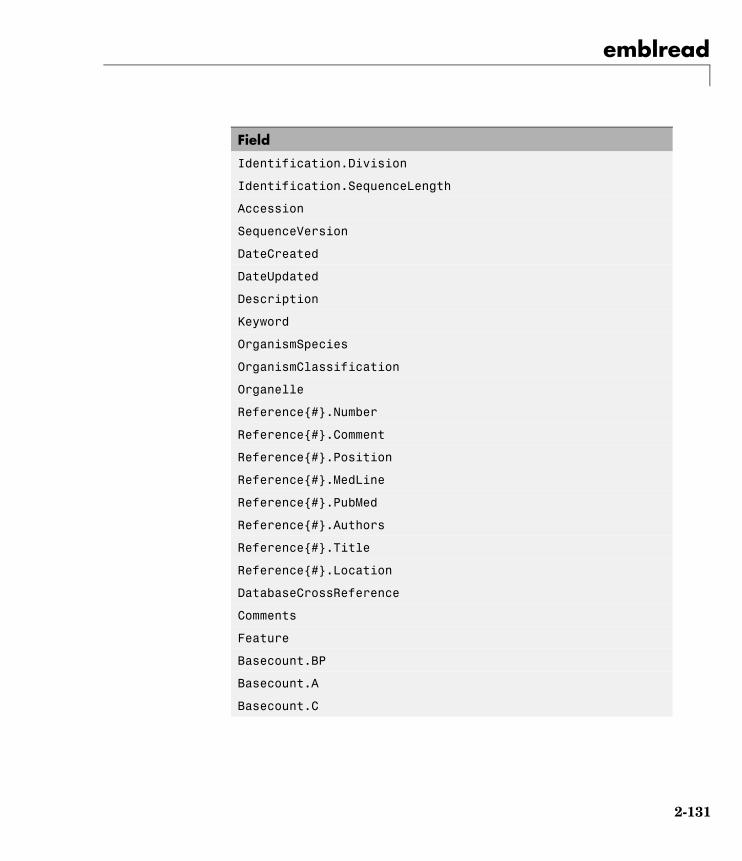
emblread
Field
Identification.Division
Identification.SequenceLength
Accession
SequenceVersion
DateCreated
DateUpdated
Description
Keyword
OrganismSpecies
OrganismClassification
Organelle
Reference{#}.Number
Reference{#}.Comment
Reference{#}.Position
Reference{#}.MedLine
Reference{#}.PubMed
Reference{#}.Authors
Reference{#}.Title
Reference{#}.Location
DatabaseCrossReference
Comments
Feature
Basecount.BP
Basecount.A
Basecount.C
2-131

emblread
Field
Basecount.G
Basecount.T
Basecount.Other
Sequence
Note Topology information was not included in EMBL flat files beforerelease 87 of the database. When reading a file created before release87, EMBLREAD returns an empty Identification.Topology field.
Note The entry name is no longer displayed in the ID line ofEMBL flat files in release 87. When reading a file created inrelease 87, EMBLREAD returns the accession number in theIdentification.EntryName field.
EMBLSeq = emblread ('File', SequenceOnly',SequenceOnlyValue), when SequenceOnlyValue is true,reads only the sequence information.
Examples Get sequence information from the Web, save to a file, and then readback into MATLAB.
getembl('X00558','ToFile','rat_protein.txt');EMBLData = emblread('rat_protein.txt')
See Also Bioinformatics Toolbox functions: fastaread, genbankread, getembl,seqtool
2-132

evalrasmolscript
Purpose Send RasMol script commands to Molecule Viewer window
Syntax evalrasmolscript(FigureHandle, Command)evalrasmolscript(FigureHandle, 'File', FileValue)
ArgumentsFigureHandle Figure handle to a molecule viewer returned by the
molviewer function.
Command Either of the following:
• String specifying one or more RasMol scriptcommands. Use a ; to separate commands.
• Character array or cell array containing stringsspecifying RasMol script commands.
Note For a complete list of RasMol scriptcommands, see
http://www.stolaf.edu/academics/chemapps/jmol/docs/
FileValue String specifying a file name or a path and file nameof a text file containing Jmol script commands. Ifyou specify only a file name, that file must be on theMATLAB search path or in the MATLAB CurrentDirectory.
Description evalrasmolscript(FigureHandle, Command) sends the RasMol scriptcommands specified by Command to FigureHandle, the figure handle of aMolecule Viewer window created using the molviewer function.
evalrasmolscript(FigureHandle, 'File', FileValue) sends theRasMol script commands specified by FileValue to FigureHandle, the
2-133
evalrasmolscript
figure handle of a Molecule Viewer window created using the molviewerfunction.
Examples 1 Use the molviewer function to create a figure handle to a MoleculeViewer window.
FH = molviewer('2DHB')
2 Use the evalrasmolscript function to send script commands to themolecule viewer that change the background to black and spin themolecule.
evalrasmolscript(FH, 'background white; spin')
See Also Bioinformatics Toolbox functions: getpdb, molviewer, pdbread,pdbwrite
2-134

exprprofrange
Purpose Calculate range of gene expression profiles
Syntax Range = exprprofrange(Data)[Range, LogRange] = exprprofrange(Data)exprprofrange(..., 'PropertyName', PropertyValue,...)exprprofrange(..., 'ShowHist', ShowHistValue)
ArgumentsData Matrix where each row corresponds to a gene.
ShowHistValue Property to control displaying a histogram withrange data. Enter either true (include rangedata) or false. The default value is false.
Description Range = exprprofrange(Data) calculates the range of each expressionprofile in a data set (Data).
[Range, LogRange] = exprprofrange(Data) returns the log range,that is, log(max(prof))- log(min(prof)), of each expression profile.If you do not specify output arguments, exprprofrange displays ahistogram bar plot of the range.
exprprofrange(..., 'PropertyName', PropertyValue,...) definesoptional properties using property name/value pairs.
exprprofrange(..., 'ShowHist', ShowHistValue), whenShowHistValue is true, displays a histogram of the range data.
Examples Calculate the range of expression profiles for yeast data as geneexpression changes during the metabolic shift from fermentation torespiration.
load yeastdatarange = exprprofrange(yeastvalues,'ShowHist',true);
See Also Bioinformatics Toolbox function exprprofvar, generangefilter
2-135

exprprofvar
Purpose Calculate variance of gene expression profiles
Syntax Variance = exprprofvar(Data)exprprofvar(..., 'PropertyName', PropertyValue,...)exprprofvar(..., 'ShowHist', ShowHistValue)
ArgumentsData Matrix where each row corresponds to a gene.
ShowHistValue Property to control the display of a histogram withvariance data. Enter either true or false (default).
Description Variance = exprprofvar(Data) calculates the variance of eachexpression profile in a data set (Data). If you do not specify outputarguments, this function displays a histogram bar plot of the range.
exprprofvar(..., 'PropertyName', PropertyValue,...) definesoptional properties using property name/value pairs.
exprprofvar(..., 'ShowHist', ShowHistValue), when ShowHist istrue, displays a histogram of the range data .
Examples Calculate the variance of expression profiles for yeast data as geneexpression changes during the metabolic shift from fermentation torespiration.
load yeastdatadatavar = exprprofvar(yeastvalues,'ShowHist',true);
See Also Bioinformatics Toolbox functions exprprofrange, generangefilter,genevarfilter
2-136

fastaread
Purpose Read data from FASTA file
Syntax FASTAData = fastaread(File)[Header, Sequence] = fastaread(File)fastaread(..., 'PropertyName', PropertyValue, ...)fastaread(..., 'IgnoreGaps', IgnoreGapsValue, ...)fastaread(..., 'Blockread', BlockreadValue, ...)
ArgumentsFile FASTA-formatted file (ASCII text file). Enter
a file name, a path and file name, or a URLpointing to a file. File can also be a MATLABcharacter array that contains the text for a filename.
FASTAData MATLAB structure with the fields Header andSequence.
IgnoreGapsValue Property to control removing gap symbols.Enter either true or false (default).
BlockreadValue Property to control reading a single entry orblock of entries from a file containing multiplesequences. Enter a scalar N, to read the Nthentry in the file. Enter a 1-by-2 vector [M1, M2],to read the block of entries starting at entry M1and ending at entry M2. To read all remainingentries in the file starting at entry M1, enter apositive value for M1 and enter Inf for M2.
Description fastaread reads data from a FASTA-formatted file into a MATLABstructure with the following fields:
Field
Header
Sequence
2-137

fastaread
A file with a FASTA format begins with a right angle bracket (>) and asingle line description. Following this description is the sequence as aseries of lines with fewer than 80 characters. Sequences are expected touse the standard IUB/IUPAC amino acid and nucleotide letter codes.
For a list of codes, see aminolookup and baselookup.
FASTAData = fastaread(File) reads a file with a FASTA formatand returns the data in a structure. FASTAData.Header is the headerinformation, while FASTAData.Sequence is the sequence stored as astring of letters.
[Header, Sequence] = fastaread(File) reads data from a fileinto separate variables. If the file contains more than one sequence,then header and sequence are cell arrays of header and sequenceinformation.
fastaread(..., 'PropertyName', PropertyValue, ...)definesoptional properties. The property name/value pairs can be in any formatsupported by the function set (for example, name-value string pairs,structures, and name-value cell array pairs).
fastaread(..., 'IgnoreGaps', IgnoreGapsValue, ...), whenIgnoreGapsValue is true, removes any gap symbol ('-' or '.') fromthe sequences. Default is false.
fastaread(..., 'Blockread', BlockreadValue, ...) lets you readin a single entry or block of entries from a file containing multiplesequences. If BlockreadValue is a scalar N, then fastaread reads theNth entry in the file. If BlockreadValue is a 1-by-2 vector [M1, M2], thenfastaread reads the block of entries starting at entry M1 and ending atentry M2. To read all remaining entries in the file starting at entry M1,enter a positive value for M1 and enter Inf for M2.
Examples Read the sequence for the human p53 tumor gene.
p53nt = fastaread('p53nt.txt')
Read the sequence for the human p53 tumor protein.
2-138

fastaread
p53aa = fastaread('p53aa.txt')
Read the human mitochondrion genome in FASTA format.
entrezSite = 'http://www.ncbi.nlm.nih.gov/entrez/viewer.fcgi?'textOptions = '&txt=on&view=fasta'genbankID = '&list_uids=NC_001807'mitochondrion = fastaread([entrezSite textOptions genbankID])
See Also Bioinformatics Toolbox functions: emblread, fastawrite, genbankread,genpeptread, multialignread, seqprofile, seqtool
2-139

fastawrite
Purpose Write to file using FASTA format
Syntax fastawrite(File, Data)fastawrite(File, Header, Sequence)
Arguments File String specifying either a file name or a path and filename supported by your operating system. If you specifyonly a file name, the file is saved to the MATLAB CurrentDirectory.
Data Any of the following:• String with a FASTA format
• Sequence object
• MATLAB structure containing the fields Header andSequence
• GenBank/GenPept structure
Header String containing information about the sequence.This text will be included in the header of theFASTA-formatted file, File.
Sequence String or name of variable containing an amino acid ornucleotide sequence using the standard IUB/IUPACletter or integer codes. For a list of valid characters, seeAmino Acid Lookup Table on page 2-42 or NucleotideLookup Table on page 2-52.
Description fastawrite(File, Data) writes the contents of Data to aFASTA-formatted file (ASCII text file).
fastawrite(File, Header, Sequence) writes the specified headerand sequence information to a FASTA-formatted file (ASCII text file).
Examples %get the sequence for the human p53 gene from GenBank.seq = getgenbank('NM_000546')
2-140

fastawrite
%find the CDS line in the FEATURES information.cdsline = strmatch('CDS',seq.Features)
%read the coordinates of the coding region.[start,stop] = strread(seq.Features(cdsline,:),'%*s%d..%d')
%extract the coding region.codingSeq = seq.Sequence(start:stop)
%write just the coding region to a FASTA file.fastawrite('p53coding.txt','Coding region for p53',codingSeq);
Save multiple sequences.
data(1).Sequence = 'ACACAGGAAA'data(1).Header = 'First sequence'data(2).Sequence = 'ACGTCAGGTC'data(2).Header = 'Second sequence'
fastawrite('my_sequences.txt', data)type('my_sequences.txt')
>First sequenceACACAGGAAA
>Second sequenceACGTCAGGTC
See Also Bioinformatics Toolbox functions: fastaread, seqtool
2-141
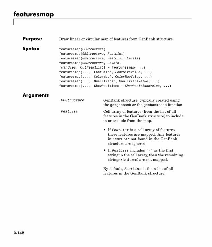
featuresmap
Purpose Draw linear or circular map of features from GenBank structure
Syntax featuresmap(GBStructure)featuresmap(GBStructure, FeatList)featuresmap(GBStructure, FeatList, Levels)featuresmap(GBStructure, Levels)[Handles, OutFeatList] = featuresmap(...)featuresmap(..., 'FontSize', FontSizeValue, ...)featuresmap(..., 'ColorMap', ColorMapValue, ...)featuresmap(..., 'Qualifiers', QualifiersValue, ...)featuresmap(..., 'ShowPositions', ShowPositionsValue, ...)
ArgumentsGBStructure GenBank structure, typically created using
the getgenbank or the genbankread function.
FeatList Cell array of features (from the list of allfeatures in the GenBank structure) to includein or exclude from the map.
• If FeatList is a cell array of features,these features are mapped. Any featuresin FeatList not found in the GenBankstructure are ignored.
• If FeatList includes '-' as the firststring in the cell array, then the remainingstrings (features) are not mapped.
By default, FeatList is the a list of allfeatures in the GenBank structure.
2-142
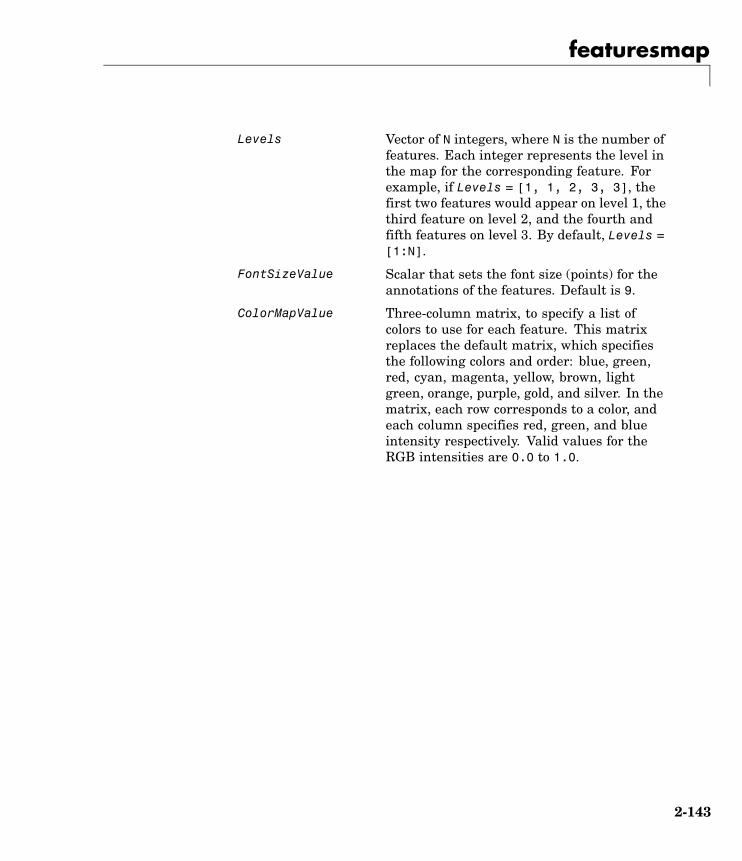
featuresmap
Levels Vector of N integers, where N is the number offeatures. Each integer represents the level inthe map for the corresponding feature. Forexample, if Levels = [1, 1, 2, 3, 3], thefirst two features would appear on level 1, thethird feature on level 2, and the fourth andfifth features on level 3. By default, Levels =[1:N].
FontSizeValue Scalar that sets the font size (points) for theannotations of the features. Default is 9.
ColorMapValue Three-column matrix, to specify a list ofcolors to use for each feature. This matrixreplaces the default matrix, which specifiesthe following colors and order: blue, green,red, cyan, magenta, yellow, brown, lightgreen, orange, purple, gold, and silver. In thematrix, each row corresponds to a color, andeach column specifies red, green, and blueintensity respectively. Valid values for theRGB intensities are 0.0 to 1.0.
2-143

featuresmap
QualifiersValue Cell array of strings to specify an ordered listof qualifiers to search for in the structureand use as annotations. For each feature,the first matching qualifier found from thelist is used for its annotation. If a featuredoes not include any of the qualifiers, noannotation displays for that feature. Bydefault, QualifiersValue = {'gene','product', 'locus_tag', 'note','db_xref', 'protein_id'}. Provide yourown QualifiersValue to limit or expand thelist of qualifiers or change the search order.
Tip Set QualifiersValue = {} to create amap with no annotations.
Tip To determine all qualifiers available fora given feature, do either of the following:
• Create the map, and then click a feature orits annotation to list all qualifiers for thatfeature.
• Use the featuresparse command to parseall the features into a new structure, andthen use the fieldnames command tolist the qualifiers for a specific feature.See Determining Qualifiers for a SpecificFeature on page 2-150.
ShowPositionsValue Property to add the sequence position tothe annotation label for each feature. Entertrue to add the sequence position. Defaultis false.
2-144

featuresmap
Description featuresmap(GBStructure) creates a linear or circular map of allfeatures from a GenBank structure, typically created using thegetgenbank or the genbankread function.
featuresmap(GBStructure, FeatList) creates a linear or circular mapof a subset of features from a GenBank structure. FeatList lets youspecify features (from the list of all features in the GenBank structure)to include in or exclude from the map.
• If FeatList is a cell array of features, these features are mapped.Any features in FeatList not found in the GenBank structure areignored.
• If FeatList includes '-' as the first string in the cell array, then theremaining strings (features) are not mapped.
By default, FeatList is a list of all features in the GenBank structure.
featuresmap(GBStructure, FeatList, Levels) orfeaturesmap(GBStructure, Levels) indicates which level on the mapeach feature is drawn. Level 1 is the left-most (linear map) or inner-most(circular map) level, and level N is the right-most (linear map) orouter-most (circular map) level, where N is the number of features.
Levels is a vector of N integers, where N is the number of features. Eachinteger represents the level in the map for the corresponding feature.For example, if Levels = [1, 1, 2, 3, 3], the first two features wouldappear on level 1, the third feature on level 2, and the fourth and fifthfeatures on level 3. By default, Levels = [1:N].
[Handles, OutFeatList] = featuresmap(...) returns a list ofhandles for each feature in OutFeatList. It also returns OutFeatList,which is a cell array of the mapped features.
Tip Use Handles and OutFeatList with the legend command to createa legend of features.
2-145
featuresmap
featuresmap(..., 'PropertyName', PropertyValue, ...) definesoptional properties that use property name/value pairs in any order.These property name/value pairs are as follows:
featuresmap(..., 'FontSize', FontSizeValue, ...) sets the font size(points) for the annotations of the features. Default FontSizeValue is 9.
featuresmap(..., 'ColorMap', ColorMapValue, ...) specifies a list ofcolors to use for each feature. This matrix replaces the default matrix,which specifies the following colors and order: blue, green, red, cyan,magenta, yellow, brown, light green, orange, purple, gold, and silver.ColorMapValue is a three-column matrix, where each row correspondsto a color, and each column specifies red, green, and blue intensityrespectively. Valid values for the RGB intensities are 0.0 to 1.0.
featuresmap(..., 'Qualifiers', QualifiersValue, ...) lets youspecify an ordered list of qualifiers to search for and use as annotations.For each feature, the first matching qualifier found from the list is usedfor its annotation. If a feature does not include any of the qualifiers, noannotation displays for that feature. QualifiersValue is a cell arrayof strings. By default, QualifiersValue = {'gene', 'product','locus_tag', 'note', 'db_xref', 'protein_id'}. Provide yourown QualifiersValue to limit or expand the list of qualifiers or changethe search order.
Tip Set QualifiersValue = {} to create a map with no annotations.
2-146

featuresmap
Tip To determine all qualifiers available for a given feature, do eitherof the following:
• Create the map, and then click a feature or its annotation to list allqualifiers for that feature.
• Use the featuresparse command to parse all the features into anew structure, and then use the fieldnames command to list thequalifiers for a specific feature. See Determining Qualifiers for aSpecific Feature on page 2-150.
featuresmap(..., 'ShowPositions', ShowPositionsValue, ...)lets you add the sequence position to the annotation label. IfShowPositionsValue is true, sequence positions are added to theannotation labels. Default is false.
2-147

featuresmap
2-148

featuresmap
2-149

featuresmap
After creating a map:
• Click a feature or annotation to display a list of all qualifiers for thatfeature.
• Zoom the plot by clicking the following buttons:
or
Examples Creating a Circular Map with Legend
The following example creates a circular map of five different featuresmapped on three levels. It also uses outputs from the featuresmapfunction as inputs to the legend function to add a legend to the map.
GBStructure = getgenbank('J01415');[Handles, OutFeatList] = featuresmap(GBStructure, ...
{'CDS','D_loop','mRNA','tRNA','rRNA'}, [1 2 2 2 3])legend(Handles, OutFeatList, 'interpreter', 'none', ...
'location','bestoutside')title('Human Mitochondrion, Complete Genome')
Creating a Linear Map with Sequence Position Labels andChanged Font Size
The following example creates a linear map showing only the genefeature. It changes the font of the labels to seven points and includesthe sequence position in the labels.
herpes = getgenbank('NC_001348');featuresmap(herpes,{'gene'},'fontsize',7,'showpositions',true)title('Genes in Human herpesvirus 3 (strain Dumas)')
Determining Qualifiers for a Specific Feature
The following example uses the getgenbank function to create aGenBank structure, GBStructure. It then uses the featuresparsefunction to parse the features in the GenBank structure into a new
2-150
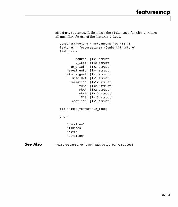
featuresmap
structure, features. It then uses the fieldnames function to returnall qualifiers for one of the features, D_loop.
GenBankStructure = getgenbank('J01415');features = featuresparse (GenBankStructure)features =
source: [1x1 struct]D_loop: [1x2 struct]
rep_origin: [1x3 struct]repeat_unit: [1x4 struct]misc_signal: [1x1 struct]
misc_RNA: [1x1 struct]variation: [1x17 struct]
tRNA: [1x22 struct]rRNA: [1x2 struct]mRNA: [1x10 struct]CDS: [1x13 struct]
conflict: [1x1 struct]
fieldnames(features.D_loop)
ans =
'Location''Indices''note''citation'
See Also featuresparse, genbankread, getgenbank, seqtool
2-151
featuresparse
Purpose Parse features from GenBank, GenPept, or EMBL data
Syntax FeatStruct = featuresparse(Features)FeatStruct = featuresparse(Features, ...'Feature',FeatureValue, ...)FeatStruct = featuresparse(Features, ...'Sequence',
SequenceValue, ...)
Arguments Features Any of the following:• String containing GenBank, GenPept, or EMBL
features
• MATLAB character array including textdescribing GenBank, GenPept, or EMBLfeatures
• MATLAB structure with fields correspondingto GenBank, GenPept, or EMBL data, such asthose returned by genbankread, genpeptread,emblread, getgenbank, getgenpept, or getembl
FeatureValue Name of a feature contained in Features. Whenspecified, featuresparse returns only thesubstructure that corresponds to this feature.If there are multiple features with the sameFeatureValue, then FeatStruct is an array ofstructures.
SequenceValue Property to control the extraction, when possible,of the sequences respective to each feature, joiningand complementing pieces of the source sequenceand storing them in the Sequence field of thereturned structure, FeatStruct. When extractingthe sequence from an incomplete CDS feature,featuresparse uses the codon_start qualifier toadjust the frame of the sequence. Choices are trueor false (default).
2-152

featuresparse
ReturnValues
FeatStruct Output structure containing a field for everydatabase feature. Each field name in FeatStructmatches the corresponding feature name in theGenBank, GenPept, or EMBL database, with theexceptions listed in the table below. Fields inFeatStruct contain substructures with featurequalifiers as fields. In the GenBank, GenPept,and EMBL databases, for each feature, theonly mandatory qualifier is its location, whichfeaturesparse translates to the field Location.When possible, featuresparse also translates thislocation to numeric indices, creating an Indicesfield.
Note If you use the Indices field to extractsequence information, you may need to complementthe sequences.
Description FeatStruct = featuresparse(Features) parses the features fromFeatures, which contains GenBank, GenPept, or EMBL features.Features can be a:
• String containing GenBank, GenPept, or EMBL features
• MATLAB character array including text describing GenBank,GenPept, or EMBL features
• MATLAB structure with fields corresponding to GenBank, GenPept,or EMBL data, such as those returned by genbankread, genpeptread,emblread, getgenbank, getgenpept, or getembl
FeatStruct is the output structure containing a field for every databasefeature. Each field name in FeatStruct matches the corresponding
2-153
featuresparse
feature name in the GenBank, GenPept, or EMBL database, with thefollowing exceptions.
Feature Name in GenBank,GenPept, or EMBL Database
Field Name in MATLAB Structure
-10_signal minus_10_signal
-35_signal minus_35_signal
3'UTR three_prime_UTR
3'clip three_prime_clip
5'UTR five_prime_UTR
5'clip five_prime_clip
D-loop D_loop
Fields in FeatStruct contain substructures with feature qualifiers asfields. In the GenBank, GenPept, and EMBL databases, for each feature,the only mandatory qualifier is its location, which featuresparsetranslates to the field Location. When possible, featuresparse alsotranslates this location to numeric indices, creating an Indices field.
Note If you use the Indices field to extract sequence information, youmay need to complement the sequences.
FeatStruct = featuresparse (Features, ...'PropertyName',PropertyValue, ...) calls featuresparse with optional propertiesthat use property name/property value pairs. You can specify one ormore properties in any order. Each PropertyName must be enclosedin single quotation marks and is case insensitive. These propertyname/property value pairs are as follows:
FeatStruct = featuresparse(Features, ...'Feature', FeatureValue,...) returns only the substructure that corresponds to FeatureValue,the name of a feature contained in Features. If there are multiple
2-154
featuresparse
features with the same FeatureValue, then FeatStruct is an array ofstructures.
FeatStruct = featuresparse(Features, ...'Sequence',SequenceValue, ...) controls the extraction, when possible, of thesequences respective to each feature, joining and complementingpieces of the source sequence and storing them in the field Sequence.When extracting the sequence from an incomplete CDS feature,featuresparse uses the codon_start qualifier to adjust the frame ofthe sequence. Choices are true or false (default).
Examples Obtaining All Features from a GenBank File
The following example obtains all the features stored in the GenBankfile nm175642.txt:
gbkStruct = genbankread('nm175642.txt');features = featuresparse(gbkStruct)
features =
source: [1x1 struct]gene: [1x1 struct]CDS: [1x1 struct]
Obtaining a Subset of Features from a GenBank Record
The following example obtains only the coding sequences (CDS) featureof the Caenorhabditis elegans cosmid record (accession number Z92777)from the GenBank database:
worm = getgenbank('Z92777');CDS = featuresparse(worm,'feature','cds')
CDS =
1x12 struct array with fields:LocationIndices
2-155

featuresparse
locus_tagstandard_namenotecodon_startproductprotein_iddb_xreftranslation
Extracting Sequences for Each Feature
1 Retrieve two nucleotide sequences from the GenBank database forthe neuraminidase (NA) protein of two strains of the Influenza Avirus (H5N1).
hk01 = getgenbank('AF509094');vt04 = getgenbank('DQ094287');
2 Extract the sequence of the coding region for the neuraminidase(NA) protein from the two nucleotide sequences. The sequences ofthe coding regions are stored in the Sequence fields of the returnedstructures, hk01_cds and vt04_cds.
hk01_cds = featuresparse(hk01,'feature','CDS','Sequence',true);vt04_cds = featuresparse(vt04,'feature','CDS','Sequence',true);
3 Once you have extracted the nucleotide sequences, you can use thent2aa and nwalign functions to align the amino acids sequencesconverted from the nucleotide sequences.
[sc,al]=nwalign(nt2aa(hk01_cds),nt2aa(vt04_cds),'extendgap',1);
4 Then you can use the seqinsertgaps function to copy the gaps fromthe aligned amino acid sequences to their corresponding nucleotidesequences, thus codon-aligning them.
hk01_aligned = seqinsertgaps(hk01_cds,al(1,:))vt04_aligned = seqinsertgaps(vt04_cds,al(3,:))
2-156

featuresparse
5 Once you have code aligned the two sequences, you can usethem as input to other functions such as dnds, which calculatesthe synonymous and nonsynonymous substitutions rates of thecodon-aligned nucleotide sequences. By setting Verbose to true, youcan also display the codons considered in the computations and theiramino acid translations.
[dn,ds] = dnds(hk01_aligned,vt04_aligned,'verbose',true)
See Also Bioinformatics Toolbox functions: emblread, genbankread,genpeptread, getgenbank, getgenpept
2-157

galread
Purpose Read microarray data from GenePix array list file
Syntax GALData = galread('File')
ArgumentsFile GenePix Array List formatted file (GAL). Enter a
file name, or enter a path and file name.
Description galread reads data from a GenePix formatted file into a MATLABstructure.
GALData = galread('File') reads in a GenePix Array List formattedfile (File ) and creates a structure (GALData) containing the followingfields:
Field
Header
BlockData
IDs
Names
The field BlockData is an N-by-3 array. The columns of this array arethe block data, the column data, and the row data respectively. Formore information on the GAL format, see
http://www.moleculardevices.com/pages/software/gn_genepix_file_formats.html#gal
For a list of supported file format versions, see
http://www.moleculardevices.com/pages/software/gn_genepix_file_formats.html
GenePix is a registered trademark of Molecular Devices Corporation.
See Also Bioinformatics Toolbox functions: affyread, geosoftread, gprread,imageneread, sptread
2-158
gcrma
Purpose Perform GC Robust Multi-array Average (GCRMA) backgroundadjustment, quantile normalization, and median-polish summarizationon Affymetrix microarray probe-level data
Syntax ExpressionMatrix = gcrma(PMMatrix, MMMatrix, ProbeIndices,AffinPM, AffinMM)
ExpressionMatrix = gcrma(PMMatrix, MMMatrix, ProbeIndices,SequenceMatrix)
ExpressionMatrix = gcrma( ...'ChipIndex',ChipIndexValue, ...)ExpressionMatrix = gcrma( ...'OpticalCorr',OpticalCorrValue,
...)ExpressionMatrix = gcrma( ...'CorrConst', CorrConstValue,
...)ExpressionMatrix = gcrma( ...'Method', MethodValue, ...)ExpressionMatrix = gcrma( ...'TuningParam',TuningParamValue,
...)ExpressionMatrix = gcrma( ...'GSBCorr', GSBCorrValue, ...)ExpressionMatrix = gcrma( ...'Normalize', NormalizeValue,
...)ExpressionMatrix = gcrma( ...'Verbose', VerboseValue, ...)
2-159
gcrma
ArgumentsPMMatrix Matrix of intensity values where each row
corresponds to a perfect match (PM) probe andeach column corresponds to an Affymetrix CELfile. (Each CEL file is generated from a separatechip. All chips should be of the same type.)
Tip You can use the PMIntensities matrixreturned by the celintensityread function.
MMMatrix Matrix of intensity values where each rowcorresponds to a mismatch (MM) probe and eachcolumn corresponds to an Affymetrix CEL file.(Each CEL file is generated from a separatechip. All chips should be of the same type.)
Tip You can use the MMIntensities matrixreturned by the celintensityread function.
ProbeIndices Column vector containing probe indices. Probeswithin a probe set are numbered 0 through N -1, where N is the number of probes in the probeset.
Tip You can use the affyprobeseqreadfunction to generate this column vector.
2-160
gcrma
AffinPM Column vector of PM probe affinities.
Tip You can use the affyprobeaffinitiesfunction to generate this column vector.
AffinMM Column vector of MM probe affinities.
Tip You can use the affyprobeaffinitiesfunction to generate this column vector.
2-161

gcrma
SequenceMatrix An N-by-25 matrix of sequence information forthe perfect match (PM) probes on the AffymetrixGeneChip array, where N is the number ofprobes on the array. Each row corresponds toa probe, and each column corresponds to oneof the 25 sequence positions. Nucleotides inthe sequences are represented by one of thefollowing integers:
• 0 — None
• 1 — A
• 2 — C
• 3 — G
• 4 — T
Tip You can use the affyprobeseqreadfunction to generate this matrix. If youhave this sequence information in letterrepresentation, you can convert it to integerrepresentation using the nt2int function.
ChipIndexValue Positive integer specifying a column indexin MMMatrix, which specifies a chip. Thischip intensity data is used to compute probeaffinities, assuming no affinity data is provided.Default is 1.
OpticalCorrValue Controls the use of optical backgroundcorrection on the PM and MM intensity valuesin PMMatrix and MMMatrix. Choices are true(default) or false.
2-162
gcrma
CorrConstValue Value that specifies the correlation constant,rho, for background intensity for each PM/MMprobe pair. Choices are any value ≥ 0 and ≤ 1.Default is 0.7.
MethodValue String that specifies the method to estimatethe signal. Choices are MLE, a faster, ad hocMaximum Likelihood Estimate method, or EB,a slower, more formal, empirical Bayes method.Default is MLE.
TuningParamValue Value that specifies the tuning parameter usedby the estimate method. This tuning parametersets the lower bound of signal values withpositive probability. Choices are a positivevalue. Default is 5 (MLE) or 0.5 (EB).
Tip For information on determining a settingfor this parameter, see Wu et al., 2004.
GSBCorrValue Controls whether gene specific binding (GSB)correction is performed on the non-specificbinding (NSB) data. Choices are true (default)or false.
NormalizeValue Controls whether quantile normalizationis performed on background adjusted data.Choices are true (default) or false.
VerboseValue Controls the display of a progress reportshowing the number of each chip as it iscompleted. Choices are true (default) or false.
2-163

gcrma
ReturnValues ExpressionMatrix Matrix of log2 expression values where each
row corresponds to a gene (probe set) and eachcolumn corresponds to an Affymetrix CEL file,which represents a single chip.
Description ExpressionMatrix = gcrma(PMMatrix, MMMatrix, ProbeIndices,AffinPM, AffinMM) performs GCRMA background adjustment,quantile normalization , and median-polish summarization onAffymetrix microarray probe-level data using probe affinity data.ExpressionMatrix is a matrix of log2 expression values where each rowcorresponds to a gene (probe set) and each column corresponds to anAffymetrix CEL file, which represents a single chip.
Note There is no column in ExpressionMatrix that contains probe setor gene information.
ExpressionMatrix = gcrma(PMMatrix, MMMatrix, ProbeIndices,SequenceMatrix) performs GCRMA background adjustment, quantilenormalization, and Robust Multi-array Average (RMA) summarizationon Affymetrix microarray probe-level data using probe sequence datato compute probe affinity data. ExpressionMatrix is a matrix of log2expression values where each row corresponds to a gene (probe set) andeach column corresponds to an Affymetrix CEL file, which represents asingle chip.
Note If AffinPM and AffinMM affinity data and SequenceMatrixsequence data are not available, you can still use the gcrma function byentering an empty matrix for these inputs in the syntax.
ExpressionMatrix = gcrma( ...'PropertyName', PropertyValue,...) calls gcrma with optional properties that use property
2-164
gcrma
name/property value pairs. You can specify one or more properties inany order. Each PropertyName must be enclosed in single quotes andis case insensitive. These property name/property value pairs are asfollows:
ExpressionMatrix = gcrma( ...'ChipIndex', ChipIndexValue,...) computes probe affinities from MM probe intensity data from thechip with the specified column index in MMMatrix, assuming no affinitydata is provided. Default ChipIndexValue is 1. If AffinPM and AffinMMaffinity data are provided, this property is ignored.
ExpressionMatrix = gcrma( ...'OpticalCorr',OpticalCorrValue, ...) controls the use of optical backgroundcorrection on the PM and MM intensity values in PMMatrix andMMMatrix. Choices are true (default) or false.
ExpressionMatrix = gcrma( ...'CorrConst', CorrConstValue,...) specifies the correlation constant, rho, for background intensityfor each PM/MM probe pair. Choices are any value ≥ 0 and ≤ 1. Defaultis 0.7.
ExpressionMatrix = gcrma( ...'Method', MethodValue, ...)specifies the method to estimate the signal. Choices are MLE, a faster,ad hoc Maximum Likelihood Estimate method, or EB, a slower, moreformal, empirical Bayes method. Default is MLE.
ExpressionMatrix = gcrma( ...'TuningParam',TuningParamValue, ...) specifies the tuning parameterused by the estimate method. This tuning parameter sets the lowerbound of signal values with positive probability. Choices are a positivevalue. Default is 5 (MLE) or 0.5 (EB).
Tip For information on determining a setting for this parameter, seeWu et al., 2004.
ExpressionMatrix = gcrma( ...'GSBCorr', GSBCorrValue, ...)controls whether gene specific binding (GSB) correction is performed
2-165
gcrma
on the non-specific binding (NSB) data. Choices are true (default) orfalse.
ExpressionMatrix = gcrma( ...'Normalize', NormalizeValue,...) controls whether quantile normalization is performed onbackground adjusted data. Choices are true (default) or false.
ExpressionMatrix = gcrma( ...'Verbose', VerboseValue, ...)controls the display of a progress report showing the number of eachchip as it is completed. Choices are true (default) or false.
Examples 1 Load the MAT file, included with Bioinformatics Toolbox, thatcontains Affymetrix data from a prostate cancer study. The variablesin the MAT file include seqMatrix, a matrix containing sequenceinformation for PM probes, pmMatrix and mmMatrix, matricescontaining PM and MM probe intensity values, and probeIndices, acolumn vector containing probe indexing information.
load prostatecancerrawdata
2 Compute the Affymetrix PM and MM probe affinities from theirsequences and MM probe intensities.
[apm, amm] = affyprobeaffinities(seqMatrix, mmMatrix(:,1),...'ProbeIndices', probeIndices);
3 Perform GCRMA background adjustment, quantile normalization,and Robust Multi-array Average (RMA) summarization on theAffymetrix microarray probe-level data and create a matrix ofexpression values.
expdata = gcrma(pmMatrix, mmMatrix, probeIndices, seqMatrix);
The prostatecancerrawdata.mat file used in this example containsdata from Best et al., 2005.
References [1] Wu, Z., Irizarry, R.A., Gentleman, R., Murillo, F.M. and Spencer, F.(2004). A Model Based Background Adjustment for Oligonucleotide
2-166
gcrma
Expression Arrays. Journal of the American Statistical Association99(468), 909–917.
[2] Wu, Z., and Irizarry, R.A. (2005). Stochastic Models Inspired byHybridization Theory for Short Oligonucleotide Arrays. Proceedings ofRECOMB 2004. J Comput Biol. 12(6), 882–93.
[3] Wu, Z., and Irizarry, R.A. (2005). A Statistical Framework for theAnalysis of Microarray Probe-Level Data. Johns Hopkins University,Biostatistics Working Papers 73.
[4] Speed, T. (2006). Background models and GCRMA. Lecture10, Statistics 246, University of California Berkeley.http://www.stat.berkeley.edu/users/terry/Classes/s246.2006/Week10/Week.
[5] Best, C.J.M., Gillespie, J.W., Yi, Y., Chandramouli, G.V.R.,Perlmutter, M.A., Gathright, Y., Erickson, H.S., Georgevich, L., Tangrea,M.A., Duray, P.H., Gonzalez, S., Velasco, A., Linehan, W.M., Matusik,R.J., Price, D.K., Figg, W.D., Emmert-Buck, M.R., and Chuaqui, R.F.(2005). Molecular alterations in primary prostate cancer after androgenablation therapy. Clinical Cancer Research 11, 6823–6834.
See Also Bioinformatics Toolbox functions: affyprobeseqread, affyread,celintensityread, gcrmabackadj, quantilenorm, rmabackadj,rmasummary
2-167

gcrmabackadj
Purpose Perform GC Robust Multi-array Average (GCRMA) backgroundadjustment on Affymetrix microarray probe-level data using sequenceinformation
Syntax PMMatrix_Adj = gcrmabackadj(PMMatrix, MMMatrix, AffinPM,AffinMM)
[PMMatrix_Adj, nsbStruct] = gcrmabackadj(PMMatrix,MMMatrix,
AffinPM, AffinMM)... = gcrmabackadj( ...'OpticalCorr',OpticalCorrValue, ...)... = gcrmabackadj( ...'CorrConst', CorrConstValue, ...)... = gcrmabackadj( ...'Method', MethodValue, ...)... = gcrmabackadj( ...'TuningParam',TuningParamValue, ...)... = gcrmabackadj( ...'AddVariance',AddVarianceValue, ...)... = gcrmabackadj( ...'Showplot', ShowplotValue, ...)... = gcrmabackadj( ...'Verbose', VerboseValue, ...)
2-168
gcrmabackadj
ArgumentsPMMatrix Matrix of intensity values where each row
corresponds to a perfect match (PM) probe andeach column corresponds to an Affymetrix CELfile. (Each CEL file is generated from a separatechip. All chips should be of the same type.)
Tip You can use the PMIntensities matrixreturned by the celintensityread function.
MMMatrix Matrix of intensity values where each rowcorresponds to a mismatch (MM) probe and eachcolumn corresponds to an Affymetrix CEL file.(Each CEL file is generated from a separatechip. All chips should be of the same type.)
Tip You can use the MMIntensities matrixreturned by the celintensityread function.
AffinPM Column vector of PM probe affinities, such asreturned by the affyprobeaffinities function.Each row corresponds to a probe.
AffinMM Column vector of MM probe affinities, such asreturned by the affyprobeaffinities function.Each row corresponds to a probe.
OpticalCorrValue Controls the use of optical background correctionon the PM and MM probe intensity values inPMMatrix and MMMatrix. Choices are true(default) or false.
2-169
gcrmabackadj
CorrConstValue Value that specifies the correlation constant,rho, for log background intensity for eachPM/MM probe pair. Choices are any value ≥ 0and ≤ 1. Default is 0.7.
MethodValue String that specifies the method to estimatethe signal. Choices are MLE, a faster, ad hocMaximum Likelihood Estimate method, or EB,a slower, more formal, empirical Bayes method.Default is MLE.
TuningParamValue Value that specifies the tuning parameter usedby the estimate method. This tuning parametersets the lower bound of signal values withpositive probability. Choices are a positivevalue. Default is 5 (MLE) or 0.5 (EB).
Tip For information on determining a settingfor this parameter, see Wu et al., 2004.
AddVarianceValue Controls whether the signal variance is addedto the weight function for smoothing low signaledge. Choices are true or false (default).
2-170

gcrmabackadj
ShowplotValue Controls the display of a plot showing the log2 ofprobe intensity values from a specified column(chip) in MMMatrix, versus probe affinities inAffinMM. Choices are true, false, or I, aninteger specifying a column in MMMatrix. If setto true, the first column in MMMatrix is plotted.Default is:
• false — When return values are specified.
• true — When return values are not specified.
VerboseValue Controls the display of a progress reportshowing the number of each chip as it iscompleted. Choices are true (default) or false.
ReturnValues PMMatrix_Adj Matrix of background adjusted PM (perfect
match) intensity values.
nsbStruct Structure containing nonspecific bindingbackground parameters, estimated from theintensities and affinities of probes on anAffymetrix GeneChip array. nsbStruct includesthe following fields:
• sigma
• mu_pm
• mu_mm
Description PMMatrix_Adj = gcrmabackadj(PMMatrix, MMMatrix, AffinPM,AffinMM) performs GCRMA background adjustment (including opticalbackground correction and nonspecific binding correction) on Affymetrixmicroarray probe-level data, using probe sequence information andreturns PMMatrix_Adj, a matrix of background adjusted PM (perfectmatch) intensity values.
2-171
gcrmabackadj
Note If AffinPM and AffinMM data are not available, you can still usethe gcrmabackadj function by entering empty column vectors for bothof these inputs in the syntax.
[PMMatrix_Adj, nsbStruct] = gcrmabackadj(PMMatrix,MMMatrix, AffinPM, AffinMM) returns nsbStruct, a structurecontaining nonspecific binding background parameters, estimated fromthe intensities and affinities of probes on an Affymetrix GeneChiparray. nsbStruct includes the following fields:
• sigma
• mu_pm
• mu_mm
... = gcrmabackadj( ...'PropertyName', PropertyValue,
...) calls gcrmabackadj with optional properties that use propertyname/property value pairs. You can specify one or more properties inany order. Each PropertyName must be enclosed in single quotationmarks and is case insensitive. These property name/property valuepairs are as follows:
... = gcrmabackadj( ...'OpticalCorr', OpticalCorrValue,
...) controls the use of optical background correction on the PM andMM probe intensity values in PMMatrix and MMMatrix. Choices aretrue (default) or false.
... = gcrmabackadj( ...'CorrConst', CorrConstValue, ...)specifies the correlation constant, rho, for log background intensity foreach PM/MM probe pair. Choices are any value ≥ 0 and ≤ 1. Defaultis 0.7.
... = gcrmabackadj( ...'Method', MethodValue, ...) specifiesthe method to estimate the signal. Choices are MLE, a faster, ad hocMaximum Likelihood Estimate method, or EB, a slower, more formal,empirical Bayes method. Default is MLE.
2-172

gcrmabackadj
... = gcrmabackadj( ...'TuningParam', TuningParamValue,
...) specifies the tuning parameter used by the estimate method. Thistuning parameter sets the lower bound of signal values with positiveprobability. Choices are a positive value. Default is 5 (MLE) or 0.5 (EB).
Tip For information on determining a setting for this parameter, seeWu et al., 2004.
... = gcrmabackadj( ...'AddVariance', AddVarianceValue,
...) controls whether the signal variance is added to the weightfunction for smoothing low signal edge. Choices are true or false(default).
... = gcrmabackadj( ...'Showplot', ShowplotValue, ...)controls the display of a plot showing the log2 of probe intensity valuesfrom a specified column (chip) in MMMatrix, versus probe affinities inAffinMM. Choices are true, false, or I, an integer specifying a columnin MMMatrix. If set to true, the first column in MMMatrix is plotted.Default is:
• false — When return values are specified.
• true — When return values are not specified.
... = gcrmabackadj( ...'Verbose', VerboseValue, ...)controls the display of a progress report showing the number of eachchip as it is completed. Choices are true (default) or false.
Examples 1 Load the MAT file, included with Bioinformatics Toolbox, thatcontains Affymetrix data from a prostate cancer study. The variablesin the MAT file include seqMatrix, a matrix containing sequenceinformation for PM probes, pmMatrix and mmMatrix, matricescontaining PM and MM probe intensity values, and probeIndices, acolumn vector containing probe indexing information.
load prostatecancerrawdata
2-173

gcrmabackadj
2 Compute the Affymetrix PM and MM probe affinities from theirsequences and MM probe intensities.
[apm, amm] = affyprobeaffinities(seqMatrix, mmMatrix(:,1),...'ProbeIndices', probeIndices);
3 Perform GCRMA background adjustment on the Affymetrixmicroarray probe-level data, creating a matrix of backgroundadjusted PM intensity values. Also, display a plot showing the log2of probe intensity values from column 3 (chip 3) in mmMatrix, versusprobe affinities in amm.
pms_adj = gcrmabackadj(pmMatrix, mmMatrix, apm, amm, 'showplot', 3);
2-174
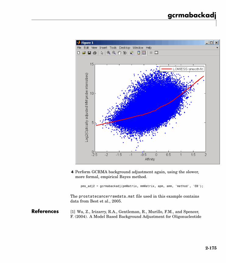
gcrmabackadj
4 Perform GCRMA background adjustment again, using the slower,more formal, empirical Bayes method.
pms_adj2 = gcrmabackadj(pmMatrix, mmMatrix, apm, amm, 'method', 'EB');
The prostatecancerrawdata.mat file used in this example containsdata from Best et al., 2005.
References [1] Wu, Z., Irizarry, R.A., Gentleman, R., Murillo, F.M., and Spencer,F. (2004). A Model Based Background Adjustment for Oligonucleotide
2-175
gcrmabackadj
Expression Arrays. Journal of the American Statistical Association99(468), 909–917.
[2] Wu, Z., and Irizarry, R.A. (2005). Stochastic Models Inspired byHybridization Theory for Short Oligonucleotide Arrays. Proceedings ofRECOMB 2004. J Comput Biol. 12(6), 882–93.
[3] Wu, Z., and Irizarry, R.A. (2005). A Statistical Framework for theAnalysis of Microarray Probe-Level Data. Johns Hopkins University,Biostatistics Working Papers 73.
[4] Wu, Z., and Irizarry, R.A. (2003). A Model BasedBackground Adjustment for Oligonucleotide ExpressionArrays. RSS Workshop on Gene Expression, Wye, England,http://biosun01.biostat.jhsph.edu/%7Eririzarr/Talks/gctalk.pdf.
[5] Abd Rabbo, N.A., and Barakat, H.M. (1979). Estimation Problemsin Bivariate Lognormal Distribution. Indian J. Pure Appl. Math 10(7),815–825.
[6] Best, C.J.M., Gillespie, J.W., Yi, Y., Chandramouli, G.V.R.,Perlmutter, M.A., Gathright, Y., Erickson, H.S., Georgevich, L., Tangrea,M.A., Duray, P.H., Gonzalez, S., Velasco, A., Linehan, W.M., Matusik,R.J., Price, D.K., Figg, W.D., Emmert-Buck, M.R., and Chuaqui, R.F.(2005). Molecular alterations in primary prostate cancer after androgenablation therapy. Clinical Cancer Research 11, 6823–6834.
See Also Bioinformatics Toolbox functions: affyprobeseqread, affyread,celintensityread, probelibraryinfo
2-176

genbankread
Purpose Read data from GenBank file
Syntax GenBankData = genbankread(File)
ArgumentsFile Either of the following:
• String specifying a file name, a path and file name,or a URL pointing to a file. The referenced file isa GenBank-formatted file (ASCII text file). If youspecify only a file name, that file must be on theMATLAB search path or in the MATLAB CurrentDirectory.
• MATLAB character array that contains the text ofa GenBank-formatted file.
GenBankData MATLAB structure with fields corresponding toGenBank keywords.
Description GenBankData = genbankread(File) reads in a GenBank-formattedfile, File, and creates a structure, GenBankData, containing fieldscorresponding to the GenBank keywords. Each separate sequence listedin the output structure GenBankData is stored as a separate elementof the structure.
Examples 1 Get sequence information for a gene (HEXA), store data in a file, andthen read back into MATLAB.
getgenbank('nm_000520', 'ToFile', 'TaySachs_Gene.txt')s = genbankread('TaySachs_Gene.txt')
s =
LocusName: 'NM_000520'LocusSequenceLength: '2255'
LocusNumberofStrands: ''
2-177
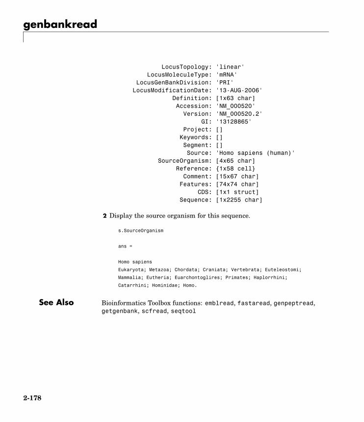
genbankread
LocusTopology: 'linear'LocusMoleculeType: 'mRNA'
LocusGenBankDivision: 'PRI'LocusModificationDate: '13-AUG-2006'
Definition: [1x63 char]Accession: 'NM_000520'
Version: 'NM_000520.2'GI: '13128865'
Project: []Keywords: []Segment: []Source: 'Homo sapiens (human)'
SourceOrganism: [4x65 char]Reference: {1x58 cell}
Comment: [15x67 char]Features: [74x74 char]
CDS: [1x1 struct]Sequence: [1x2255 char]
2 Display the source organism for this sequence.
s.SourceOrganism
ans =
Homo sapiens
Eukaryota; Metazoa; Chordata; Craniata; Vertebrata; Euteleostomi;
Mammalia; Eutheria; Euarchontoglires; Primates; Haplorrhini;
Catarrhini; Hominidae; Homo.
See Also Bioinformatics Toolbox functions: emblread, fastaread, genpeptread,getgenbank, scfread, seqtool
2-178

geneentropyfilter
Purpose Remove genes with low entropy expression values
Syntax Mask = geneentropyfilter(Data)[Masks, FData] = geneentropyfilter(Data)[Mask, FData, FNames] = geneentropyfilter(Data,Names)geneentropyfilter(..., 'PropertyName', PropertyValue,...)geneentropyfilter(..., 'Percentile', PercentileValue)
ArgumentsData Matrix where each row corresponds to the
experimental results for one gene. Each columnis the results for all genes from one experiment.
Names Cell array with the name of a gene for each rowof experimental data. Names has same numberof rows as Data with each row containing thename or ID of the gene in the data set.
PercentileValue Property to specify a percentile below which genedata is removed. Enter a value from 0 to 100.
Description Mask = geneentropyfilter(Data) identifies gene expression profilesin Data with entropy values less than the 10th percentile.
Mask is a logical vector with one element for each row in Data. Theelements of Mask corresponding to rows with a variance greater thanthe threshold have a value of 1, and those with a variance less thenthe threshold are 0.
[Masks, FData] = geneentropyfilter(Data) returns a filtereddata matrix (FData). FData can also be created using FData =Data(find(I),:).
[Mask, FData, FNames] = geneentropyfilter(Data,Names) returnsa filtered names array (FNames). You can also create FNames usingFNames = Names(I).
geneentropyfilter(..., 'PropertyName', PropertyValue,...)defines optional properties using property name/value pairs.
2-179

geneentropyfilter
geneentropyfilter(..., 'Percentile', PercentileValue)removes from the experimental data (Data) gene expression profileswith entropy values less than a given percentile (PercentileValue).
Examples load yeastdata[fyeastvalues, fgenes] = geneentropyfilter(yeastvalues,genes);
References [1] Kohane I.S., Kho A.T., Butte A.J. (2003), Microarrays for anIntegrative Genomics, Cambridge, MA:MIT Press.
See Also Bioinformatics Toolbox functions: exprprofrange, exprprofvar,genelowvalfilter, generangefilter, genevarfilter
2-180

genelowvalfilter
Purpose Remove gene profiles with low absolute values
Syntax Mask = genelowvalfilter(Data)[Mask, FData] = genelowvalfilter(Data)[Mask, FData, FNames] = genelowvalfilter(Data, Names)genelowvalfilter(..., 'PropertyName', PropertyValue,...)genelowvalfilter(..., 'Prctile', PrctileValue)genelowvalfilter(..., 'AbsValue', AbsValueValue)genelowvalfilter(..., 'AnyVal', AnyValValue)
ArgumentsData Matrix where each row corresponds to the
experimental results for one gene. Each columnis the results for all genes from one experiment.
Names Cell array with the same number of rows asData. Each row contains the name or ID of thegene in the data set.
PrctileValue Property to specify a percentile below whichgene expression profiles are removed. Enter avalue from 0 to 100.
AbsValueValue Property to specify an absolute value belowwhich gene expression profiles are removed.
AnyValValue Property to select the minimum or maximumabsolute value for comparison withAbsValueValue. If AnyValValue is true, selectsthe minimum absolute value. If AnyValValueis false, selects the maximum absolute value.The default value is false.
Description Gene expression profile experiments have data where the absolutevalues are very low. The quality of this type of data is often bad due tolarge quantization errors or simply poor spot hybridization.
Mask = genelowvalfilter(Data) identifies gene expression profiles inData with all absolute values less than the 10th percentile.
2-181
genelowvalfilter
Mask is a logical vector with one element for each row in Data. Theelements of Mask corresponding to rows with absolute expression levelsgreater than the threshold have a value of 1, and those with absoluteexpression levels less then the threshold are 0.
[Mask, FData] = genelowvalfilter(Data) returns a filtered datamatrix (FData). You can create FData using FData = Data(find(I),:).
[Mask, FData, FNames] = genelowvalfilter(Data, Names)returns a filtered names array (FNames), where Names is a cell array ofthe names of the genes corresponding to each row of Data. You can alsocreate FNames using FNames = Names(I).
genelowvalfilter(..., 'PropertyName', PropertyValue,...)defines optional properties using property name/value pairs.
genelowvalfilter(..., 'Prctile', PrctileValue) removes fromthe experimental data (Data) gene expression profiles with all absolutevalues less than a specified percentile (Percentile).
genelowvalfilter(..., 'AbsValue', AbsValueValue) calculates themaximum absolute value for each gene expression profile and removesthe profiles with maximum absolute values less than AbsValValue.
genelowvalfilter(..., 'AnyVal', AnyValValue), whenAnyValValue is true, calculates the minimum absolute value foreach gene expression profile and removes the profiles with minimumabsolute values less than AnyValValue.
Examples [data, labels, I, FI] = genelowvalfilter(data,labels,'AbsValue',5);
References [1] Kohane I.S., Kho A.T., Butte A.J. (2003), Microarrays for anIntegrative Genomics, Cambridge, MA:MIT Press.
See Also Bioinformatics Toolbox functions: exprprofrange, exprprofvar,geneentropyfilter, generangefilter, genevarfilter
2-182

geneont
Purpose Create geneont object
Syntax GeneontObj = geneontGeneontObj = geneont('File', FileValue)GeneontObj = geneont('Live', LiveValue)GeneontObj = geneont('Live', LiveValue,'ToFile', ToFileValue)
ArgumentsFileValue file name of an OBO-formatted file that is on the
MATLAB search path.
LiveValue Property to create the most up-to-date geneont object.Enter true to create a geneont object (GeneontObj)from the most recent version of the Gene Ontologydatabase. Default is false.
ToFileValue file name to which to save the geneont object from theGene Ontology database.
Description GeneontObj = geneont searches for the file gene_ontology.obo in theMATLAB Current Directory and creates a geneont object.
GeneontObj = geneont('File', FileValue) creates a geneont object(GeneontObj) from an OBO-formatted file that is on the MATLABsearch path.
GeneontObj = geneont('Live', LiveValue), when LiveValue istrue, creates a geneont object (GeneontObj) from the most recentversion of the Gene Ontology database, which is the file at
http://www.geneontology.org/ontology/gene_ontology.obo
Note The full Gene Ontology database may take several minutes todownload when you run this function using the Live property.
2-183
geneont
GeneontObj = geneont('Live', LiveValue,'ToFile', ToFileValue), when LiveValue is true, creates a geneontobject (GeneontObj) from the file at
http://www.geneontology.org/ontology/gene_ontology.obo
and saves the file to a local file (’ToFileValue’).
Examples 1 Download the Gene Ontology database from the Web into MATLAB.
GO = geneont('LIVE', true);
MATLAB creates a geneont object and displays the number of termsin the database.
Gene Ontology object with 20005 Terms.
2 Display information about the geneont object.
get(GO)
default_namespace: 'gene_ontology'format_version: '1.0'
date: '01:11:2005 16:51'Terms: [20005x1 geneont.term]
3 Search for all GO terms in the geneont object that contain the stringribosome in the property field name and create a structure of thoseterms.
comparison = regexpi(get(GO.Terms,'name'),'ribosome');indices = find(~cellfun('isempty',comparison));terms_with_ribosmome = GO.Term(indices)23x1 struct array with fields:
idnameontologydefinitionsynonym
2-184

geneont
is_apart_ofobsolete
See Also Bioinformatics Toolbox functions: goannotread, num2goid
Bioinformatics Toolbox object: geneont object
Bioinformatics Toolbox methods of geneont object: getancestors,getdescendants, getmatrix, getrelatives
2-185
generangefilter
Purpose Remove gene profiles with small profile ranges
Syntax Mask = generangefilter(Data)[Mask, FData] = generangefilter(Data)[Mask, FData, FNames] = generangefilter(Data,Names)generangefilter(..., 'PropertyName', PropertyValue,...)generangefilter(..., 'Percentile', PercentileValue)generangefilter(..., 'AbsValue', AbsValueValue)generangefilter(..., 'LOGPercentile', LOGPercentileValue)generangefilter(..., 'LOGValue', LOGValueValue)
ArgumentsData Matrix where each row corresponds to the
experimental results for one gene. Eachcolumn is the results for all genes from oneexperiment.
Names Cell array with the name of a gene for eachrow of experimental data. Names has samenumber of rows as Data with each rowcontaining the name or ID of the gene in thedata set.
PercentileValue Property to specify a percentile below whichgene expression profiles are removed. Entera value from 0 to 100.
AbsValueValue Property to specify an absolute value belowwhich gene expression profiles are removed.
LOGPercentileValue Property to specify the LOG of a percentile.
LOGValueValue Property to specify the LOG of an absolutevalue.
Description Mask = generangefilter(Data) calculates the range for each geneexpression profile in the experimental data (Data), and then identifiesthe expression profiles with ranges less than the 10th percentile.
2-186

generangefilter
Mask is a logical vector with one element for each row in Data. Theelements of Mask corresponding to rows with a range greater thenthe threshold have a value of 1, and those with a range less then thethreshold are 0.
[Mask, FData] = generangefilter(Data) returns a filtereddata matrix (FData). FData can also be created using FData =Data(find(I),:).
[Mask, FData, FNames] = generangefilter(Data,Names) returnsa filtered names array (FNames), where Names is a cell array with thenames of the genes corresponding to each row in Data. You can alsocreate FNames using FNames = Names(I).
generangefilter(..., 'PropertyName', PropertyValue,...)defines optional properties using property name/value pairs.
generangefilter(..., 'Percentile', PercentileValue) removesfrom the experimental data (Data) gene expression profiles with rangesless than a specified percentile (PercentileValue).
generangefilter(..., 'AbsValue', AbsValueValue) removes fromData gene expression profiles with ranges less than AbsValueValue.
generangefilter(..., 'LOGPercentile', LOGPercentileValue)filters genes with profile ranges in the lowest percent of the log range(LOGPercentileValue).
generangefilter(..., 'LOGValue', LOGValueValue) filters geneswith profile log ranges lower than LOGValueValue.
Examples load yeastdata
[mask, fyeastvalues, fgenes] = generangefilter(yeastvalues,genes);
References [1] Kohane I.S., Kho A.T., Butte A.J. (2003), Microarrays for anIntegrative Genomics, Cambridge, MA:MIT Press.
See Also Bioinformatics Toolbox functions: exprprofrange, exprprofvar,geneentropyfilter, genelowvalfilter, genevarfilter
2-187

geneticcode
Purpose Nucleotide codon to amino acid mapping
Syntax Map = geneticcodegeneticcode(GeneticCode)
Arguments GeneticCode Enter a code number or code name from the table .If you use a code name, you can truncate the nameto the first two characters of the name.
Genetic Code
CodeNumber
Code Name
1 Standard
2 Vertebrate Mitochondrial
3 Yeast Mitochondrial
4 Mold, Protozoan, Coelenterate Mitochondrial,and Mycoplasma/Spiroplasma
5 Invertebrate Mitochondrial
6 Ciliate, Dasycladacean, and Hexamita Nuclear
9 Echinoderm Mitochondrial
10 Euplotid Nuclear
11 Bacterial and Plant Plastid
12 Alternative Yeast Nuclear
13 Ascidian Mitochondrial
14 Flatworm Mitochondrial
15 Blepharisma Nuclear
16 Chlorophycean Mitochondrial
2-188
geneticcode
CodeNumber
Code Name
21 Trematode Mitochondrial
22 Scenedesmus Obliquus Mitochondrial
23 Thraustochytrium Mitochondrial
Description Map = geneticcode returns a structure with a mapping of nucleotidecodons to amino acids for the standard genetic code.
geneticcode(GeneticCode) returns a structure of the mapping foralternate genetic codes, where GeneticCode is either of the following:
• The transl_table (code) number from the NCBI Genetics Web page
http://www.ncbi.nlm.nih.gov/Taxonomy/Utils/wprintgc.cgi?mode=c
• One of the supported names in the table above
Examples List the mapping of nucleotide codons to amino acids for a specificgenetic code.
wormcode = geneticcode('Flatworm Mitochondrial');
See Also Bioinformatics Toolbox functions: aa2nt, aminolookup, baselookup,codonbias, dnds, dndsml, nt2aa, revgeneticcode, seqshoworfs,seqtool
2-189

genevarfilter
Purpose Filter genes with small profile variance
Syntax Mask = genevarfilter(Data)[Mask, FData] = genevarfilter(Data)[Mask, FData, FNames] = genevarfilter(Data,Names)genevarfilter(..., 'PropertyName', PropertyValue,...)genevarfilter(..., 'Percentile', PercentileValue)genevarfilter(..., 'AbsValue', AbsValValue)
ArgumentsData Matrix where each row corresponds to a gene. The first
column is the names of the genes, and each additionalcolumn is the results from an experiment.
Names Cell array with the name of a gene for each row ofexperimental data. Names has same number of rows asData with each row containing the name or ID of thegene in the data set.
Percentile Property to specify a percentile below which geneexpression profiles are removed. Enter a value from0 to 100.
AbsValue Property to specify an absolute value below which geneexpression profiles are removed.
Description Gene profiling experiments have genes that exhibit little variation inthe profile and are generally not of interest in the experiment. Thesegenes are commonly removed from the data.
Mask = genevarfilter(Data) calculates the variance for each geneexpression profile in Data and then identifies the expression profileswith a variance less than the 10th percentile.
Mask is a logical vector with one element for each row in Data. Theelements of Mask corresponding to rows with a variance greater thanthe threshold have a value of 1, and those with a variance less thanthe threshold are 0.
2-190
genevarfilter
[Mask, FData] = genevarfilter(Data) returns the filtereddata matrix (FData). You can also create FData using FData =Data(find(I),:).
[Mask, FData, FNames] = genevarfilter(Data,Names) returns afiltered names array (FNames). Names is a cell array of the names of thegenes corresponding to each row of Data. FNames can also be createdusing FNames = Names(I).
genevarfilter(..., 'PropertyName', PropertyValue,...) definesoptional properties using property name/value pairs.
genevarfilter(..., 'Percentile', PercentileValue) removesfrom the experimental data (Data) gene expression profiles with avariance less than the percentile (Percentile).
genevarfilter(..., 'AbsValue', AbsValValue) removes from Datagene expression profiles with a variance less than AbsValue.
Examples load yeastdata[fyeastvalues, fgenes] = genevarfilter(yeastvalues,genes);
References [1] Kohane I.S., Kho A.T., Butte A.J. (2003), Microarrays for anIntegrative Genomics, Cambridge, MA:MIT Press.
See Also Bioinformatics Toolbox functions: exprprofrange, exprprofvar,generangefilter, geneentropyfilter, genelowvalfilter
2-191
genpeptread
Purpose Read data from GenPept file
Syntax GenPeptData = genpeptread('File')
Arguments File GenPept formatted file (ASCII text file). Enter a filename, a path and file name, or a URL pointing to afile. File can also be a MATLAB character array thatcontains the text of a GenPept file.
Description genpeptread reads data from a GenPept formatted file into a MATLABstructure.
Note NCBI has changed the name of their protein search enginefrom GenPept to Entrez Protein. However, the function names inBioinformatics Toolbox (getgenpept and genpeptread) are unchangedrepresenting the still-used GenPept report format.
GenPeptData = genpeptread('File') reads in the GenPept formattedsequence from File and creates a structure GenPeptData, containingfields corresponding to the GenPept keywords. Each separate sequencelisted in File is stored as a separate element of the structure.GenPeptDATA contains these fields:
Field
LocusName
LocusSequenceLength
LocusMoleculeType
LocusGenBankDivision
LocusModificationDate
Definition
2-192

genpeptread
Field
Accession
PID
Version
GI
DBSource
Keywords
Source
SourceDatabase
SourceOrganism
Reference.Number
Reference.Authors
Reference.Title
Reference.Journal
Reference.MedLine
Reference.PubMed
Reference.Remark
Comment
Features
Weight
Length
Sequence
Examples Get sequence information for the protein coded by the gene HEXA, saveto a file, and then read back into MATLAB.
getgenpept('p06865', 'ToFile', 'TaySachs_Protein.txt')genpeptread('TaySachs_Protein.txt')
2-193

genpeptread
See Also Bioinformatics Toolbox functions: fastaread, genbankread,getgenpept, pdbread, seqtool
2-194
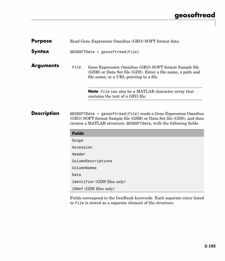
geosoftread
Purpose Read Gene Expression Omnibus (GEO) SOFT format data
Syntax GEOSOFTData = geosoftread(File)
Arguments File Gene Expression Omnibus (GEO) SOFT format Sample file(GSM) or Data Set file (GDS). Enter a file name, a path andfile name, or a URL pointing to a file.
Note File can also be a MATLAB character array thatcontains the text of a GEO file.
Description GEOSOFTData = geosoftread(File) reads a Gene Expression Omnibus(GEO) SOFT format Sample file (GSM) or Data Set file (GDS), and thencreates a MATLAB structure, GEOSOFTdata, with the following fields.
Fields
Scope
Accession
Header
ColumnDescriptions
ColumnNames
Data
Identifier (GDS files only)
IDRef (GDS files only)
Fields correspond to the GenBank keywords. Each separate entry listedin File is stored as a separate element of the structure.
2-195

geosoftread
Examples Get data from the GEO Web site and save it to a file.
geodata = getgeodata('GSM3258','ToFile','GSM3258.txt');
Use geosoftread to access a local copy of a GEO file instead of accessingit from the GEO Web site.
geodata = geosoftread('GSM3258.txt')
See Also Bioinformatics Toolbox functions: galread, getgeodata, gprread,sptread
2-196
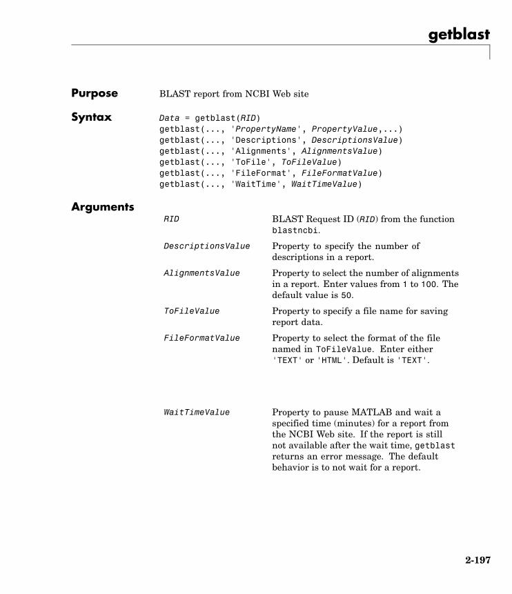
getblast
Purpose BLAST report from NCBI Web site
Syntax Data = getblast(RID)getblast(..., 'PropertyName', PropertyValue,...)getblast(..., 'Descriptions', DescriptionsValue)getblast(..., 'Alignments', AlignmentsValue)getblast(..., 'ToFile', ToFileValue)getblast(..., 'FileFormat', FileFormatValue)getblast(..., 'WaitTime', WaitTimeValue)
ArgumentsRID BLAST Request ID (RID) from the function
blastncbi.
DescriptionsValue Property to specify the number ofdescriptions in a report.
AlignmentsValue Property to select the number of alignmentsin a report. Enter values from 1 to 100. Thedefault value is 50.
ToFileValue Property to specify a file name for savingreport data.
FileFormatValue Property to select the format of the filenamed in ToFileValue. Enter either'TEXT' or 'HTML'. Default is 'TEXT'.
WaitTimeValue Property to pause MATLAB and wait aspecified time (minutes) for a report fromthe NCBI Web site. If the report is stillnot available after the wait time, getblastreturns an error message. The defaultbehavior is to not wait for a report.
2-197
getblast
Description BLAST (Basic Local Alignment Search Tool) reports offer a fast andpowerful comparative analysis of interesting protein and nucleotidesequences against known structures in existing online databases.getblast parses NCBI BLAST reports, including BLASTN, BLASTP,BLASTX, TBLASTN, TBLASTX, and psi-BLAST.
Data = getblast(RID) reads a BLAST Request ID (RID) and returnsthe report data in a structure (Data). The NCBI Request ID (RID) mustbe a recently generated report because NCBI purges reports after 24hours.
getblast(..., 'PropertyName', PropertyValue,...) definesoptional properties using property name/value pairs.
getblast(..., 'Descriptions', DescriptionsValue) includes thespecified number of descriptions (DescriptionsValue) in the report.
getblast(..., 'Alignments', AlignmentsValue) includes thespecified number of alignments in the report.
getblast(..., 'ToFile', ToFileValue) saves the data returnedfrom the NCBI BLAST report to a file (ToFileValue). The defaultformat for the file is text, but you can specify HTML with the propertyFileFormat.
getblast(..., 'FileFormat', FileFormatValue) returns the reportin the specified format (FileFormatValue).
getblast(..., 'WaitTime', WaitTimeValue) pauses MATLAB andwaits a specified time (minutes) for a report from the NCBI Web site. Ifthe report is still unavailable after the wait time, getblast returns anerror message. The default behavior is to not wait for a report.
For more information about reading and interpreting BLAST reports,see:
http://www.ncbi.nlm.nih.gov/Education/BLASTinfo/tut1.html
Examples 1 Run a BLAST search with an NCBI accession number.
RID = blastncbi('AAA59174','blastp','expect',1e-10)
2-198
getblast
2 Pass the RID to GETBLAST to parse the report, load it into aMATLAB structure, and save a copy as a text file.
report = getblast(RID,'TOFILE','Report.txt')
See Also Bioinformatics Toolbox functions: blastncbi, blastread
2-199

getembl
Purpose Sequence information from EMBL database
Syntax Data = getembl('AccessionNumber)getembl(..., 'PropertyName', PropertyValue,...)getembl(..., 'ToFile', ToFileValue)getembl(..., 'SequenceOnly', SequenceOnlyValue)
Arguments AccessionNumber Unique identifier for a sequence record. Enter aunique combination of letters and numbers.
ToFileValue Property to specify the location and file namefor saving data. Enter either a file name or apath and file name supported by your system(ASCII text file).
SequenceOnlyValue Property to control getting a sequence withoutthe metadata. Enter either true or false(default).
Description getembl retrieves information from the European Molecular BiologyLaboratory (EMBL) database for nucleotide sequences. This database ismaintained by the European Bioinformatics Institute (EBI). For moredetails about the EMBL-Bank database, see
http://www.ebi.ac.uk/embl/Documentation/index.html
Data = getembl('AccessionNumber) searches for the accessionnumber in the EMBL database (http://www.ebi.ac.uk/embl) andreturns a MATLAB structure containing the following fields:
Field
Comments
Identification
Accession
2-200

getembl
Field
SequenceVersion
DateCreated
DateUpdated
Description
Keyword
OrganismSpecies
OrganismClassification
Organelle
Reference
DatabaseCrossReference
Feature
BaseCount
Sequence
getembl(..., 'PropertyName', PropertyValue,...) definesoptional properties using property name/value pairs.
getembl(..., 'ToFile', ToFileValue) returns a structurecontaining information about the sequence and saves the information ina file using an EMBL data format. If you do not give a location or pathto the file, the file is stored in the MATLAB current directory. Read anEMBL formatted file back into MATLAB using the function emblread.
getembl(..., 'SequenceOnly', SequenceOnlyValue) , ifSequenceOnlyValue is true, returns the sequence information withoutthe metadata.
Examples Retrieve data for the rat liver apolipoprotein A-I.
emblout = getembl('X00558')
2-201
getembl
Retrieve data for the rat liver apolipoprotein and save in the filerat_protein. If a file name is given without a path, the file is stored inthe current directory.
Seq = getembl('X00558','ToFile','c:\project\rat_protein.txt')
Retrieve only the sequence for the rat liver apolipoprotein.
Seq = getembl('X00558','SequenceOnly',true)
See Also Bioinformatics Toolbox functions: emblread, getgenbank, getgenpept,getpdb, seqtool
2-202

getgenbank
Purpose Sequence information from GenBank database
Syntax Data = getgenbank('AccessionNumber')getgenbank('AccessionNumber')getgenbank(..., 'PropertyName', PropertyValue,...)getgenbank(..., 'ToFile', ToFileValue)getgenbank(..., 'FileFormat', FileFormatValue)getgenbank(..., 'SequenceOnly', SequenceOnlyValue)
ArgumentsAccessionNumber Unique identifier for a sequence record. Enter
a unique combination of letters and numbers.
ToFileValue Property to specify the location and file namefor saving data. Enter either a file name or apath and file name supported by your system(ASCII text file).
FileFormatValue Property to select the format for the filespecified with the property ToFileValue. Entereither 'GenBank' or 'FASTA'.
SequenceOnlyValue Property to control getting the sequence only.Enter either true or false.
Description getgenbank retrieves nucleotide and amino acid sequence informationfrom the GenBank database. This database is maintained by theNational Center for Biotechnology Information (NCBI). For more detailsabout the GenBank database, see
http://www.ncbi.nlm.nih.gov/Genbank/
Data = getgenbank('AccessionNumber') searches for the accessionnumber in the GenBank database and returns a MATLAB structurecontaining information for the sequence. If an error occurs whileretrieving the GenBank formatted information, then an attempt ismake to retrieve the FASTA formatted data.
2-203

getgenbank
getgenbank('AccessionNumber') displays information in theMATLAB Command Window without returning data to a variable. Thedisplayed information includes hyperlinks to the URLs for searchingand retrieving data.
getgenbank(..., 'PropertyName', PropertyValue,...) definesoptional properties using property name/value pairs.
getgenbank(..., 'ToFile', ToFileValue) saves the data returnedfrom GenBank in a file. If you do not give a location or path to the file,the file is stored in the MATLAB current directory. Read a GenBankformatted file back into MATLAB using the function genbankread.
getgenbank(..., 'FileFormat', FileFormatValue) returns thesequence in the specified format (FileFormatValue).
getgenbank(..., 'SequenceOnly', SequenceOnlyValue) whenSequenceOnly is true, returns only the sequence as a character array.When the properties SequenceOnly and ToFile are used together, theoutput file is in the FASTA format.
Examples To retrieve the sequence from chromosome 19 that codes for thehuman insulin receptor and store it in a structure, S, in the MATLABCommand Window, type:
S = getgenbank('M10051')
S =
LocusName: 'HUMINSR'
LocusSequenceLength: '4723'
LocusNumberofStrands: ''
LocusTopology: 'linear'
LocusMoleculeType: 'mRNA'
LocusGenBankDivision: 'PRI'
LocusModificationDate: '06-JAN-1995'
Definition: 'Human insulin receptor mRNA, complete cds.'
Accession: 'M10051'
Version: 'M10051.1'
2-204
getgenbank
GI: '186439'
Project: []
Keywords: 'insulin receptor; tyrosine kinase.'
Segment: []
Source: 'Homo sapiens (human)'
SourceOrganism: [4x65 char]
Reference: {[1x1 struct]}
Comment: [14x67 char]
Features: [51x74 char]
CDS: [1x1 struct]
Sequence: [1x4723 char]
SearchURL: [1x10⁵ char]
RetrieveURL: [1x95 char]
See Also Bioinformatics Toolbox functions: genbankread, getembl, getgenpept,getpdb,seqtool
2-205
getgenpept
Purpose Retrieve sequence information from GenPept database
Syntax Data = getgenpept('AccessionNumber')getgenpept(...)getgenpept(..., 'PropertyName', PropertyValue,...)getgenpept(..., 'ToFile', ToFileValue)getgenpept(..., 'FileFormat', FileFormatValue)getgenpept(..., 'SequenceOnly', SequenceOnlyValue)
Arguments AccessionNumber Unique identifier for a sequence record. Enter acombination of letters and numbers.
ToFileValue Property to specify the location and file namefor saving data. Enter either a file name or apath and file name supported by your system(ASCII text file).
FileFormatValue Property to select the format for the file specifiedwith the property ToFileValue. Enter either'GenBank' or 'FASTA'.
SequenceOnlyValue Property to control getting the sequence withoutmetadata. Enter either true or false.
Description getgenpept retrieves a protein (amino acid) sequence and sequenceinformation from the GenPept database. This database is a translationof the nucleotide sequences in GenBank and is maintained by theNational Center for Biotechnology Information (NCBI).
Note NCBI has changed the name of their protein search enginefrom GenPept to Entrez Protein. However, the function names inBioinformatics Toolbox (getgenpept and genpeptread) are unchangedrepresenting the still-used GenPept report format.
2-206

getgenpept
For more details about the GenBank database, see
http://www.ncbi.nlm.nih.gov/Genbank/
Data = getgenpept('AccessionNumber') searches for the accessionnumber in the GenPept database and returns a MATLAB structurecontaining for the sequence. If an error occurs while retrieving theGenBank formatted information, then an attempt is make to retrievethe FASTA formatted data.
getgenpept(...) displays the information to the screen withoutreturning data to a variable. The displayed information includeshyperlinks to the URLs used to search for and retrieve the data.
getgenpept(..., 'PropertyName', PropertyValue,...) definesoptional properties using property name/value pairs.
getgenpept(..., 'ToFile', ToFileValue) saves the information ina file. If you do not give a location or path to the file, the file is storedin the MATLAB current directory. Read a GenPept formatted file backinto MATLAB using the function genpeptread
getgenpept(..., 'FileFormat', FileFormatValue) returns thesequence in the specified format FileFormatValue.
getgenpept(..., 'SequenceOnly', SequenceOnlyValue)returns only the sequence information without the metadata ifSequenceOnlyValue is true. When the properties SequenceOnly andToFile are used together, the output file is in the FASTA format.
Examples To retrieve the sequence for the human insulin receptor and store it in astructure, Seq, in the MATLAB Command Window, type:
Seq = getgenpept('AAA59174')
Seq =
LocusName: 'AAA59174'LocusSequenceLength: '1382'
LocusNumberofStrands: ''
2-207

getgenpept
LocusTopology: 'linear'LocusMoleculeType: ''
LocusGenBankDivision: 'PRI'LocusModificationDate: '06-JAN-1995'
Definition: 'insulin receptor precursor.'Accession: 'AAA59174'
Version: 'AAA59174.1'GI: '307070'
Project: []DBSource: 'locus HUMINSR accession M10051.1'Keywords: ''
Source: 'Homo sapiens (human)'SourceOrganism: [4x65 char]
Reference: {[1x1 struct]}Comment: [14x67 char]
Features: [40x64 char]Sequence: [1x1382 char]
SearchURL: [1x10⁴ char]RetrieveURL: [1x92 char]
See Also Bioinformatics Toolbox functions: genpeptread, getembl, getgenbank,getpdb
2-208
getgeodata
Purpose Retrieve Gene Expression Omnibus (GEO) Sample (GSM) data
Syntax Data = getgeodata('AccessionNumber')getgeodata(..., 'PropertyName', PropertyValue,...)getgeodata(..., 'ToFile', ToFileValue)
Arguments AccessionNumber Unique identifier for a sequence record. Enter acombination of letters and numbers.
ToFileValue Property to specify the location and file namefor saving data. Enter either a file name, or apath and file name supported by your system(ASCII text file).
Description Data = getgeodata('AccessionNumber') searches for the accessionnumber in the Gene Expression Omnibus database and returns aMATLAB structure containing the following fields:
Field
Scope
Accession
Header
ColumnDescriptions
ColumnNames
Data
getgeodata(..., 'PropertyName', PropertyValue,...) definesoptional properties using property name/value pairs.
getgeodata(..., 'ToFile', ToFileValue) saves the data returnedfrom the database to a file. Read a GenPept formatted file back intoMATLAB using the function gensoftread.
2-209

getgeodata
Note Currently, Bioinformatics Toolbox supports only Sample (GSM)records.
For more information, see
http://www.ncbi.nlm.nih.gov/About/disclaimer.html
Examples geoStruct = getgeodata('GSM1768')
See Also Bioinformatics Toolbox functions: geosoftread, getgenbank,getgenpept
2-210

gethmmalignment
Purpose Retrieve multiple sequence alignment associated with hidden Markovmodel (HMM) profile from PFAM database
Syntax AlignStruct = gethmmalignment(PFAMNumber)AlignStruct = gethmmalignment(PFAMAccessNumber)AlignStruct = gethmmalignment(..., 'ToFile',ToFileValue, ...)AlignStruct = gethmmalignment(..., 'Type', TypeValue, ...)AlignStruct = gethmmalignment(..., 'Mirror', MirrorValue,
...)AlignStruct = gethmmalignment(..., 'IgnoreGaps',IgnoreGaps,
...)
ArgumentsPFAMNumber Integer specifying a protein family number of an
HMM profile record in the PFAM database. Forexample, 2 is the protein family number for theprotein family PF0002.
PFAMAccessNumber String specifying a protein family accessionnumber of an HMM profile record in the PFAMdatabase. For example, PF00002.
ToFileValue String specifying a file name or a path and filename for saving the data. If you specify only afile name, that file will be saved in the MATLABCurrent Directory.
TypeValue String that specifies the set of alignmentsreturned. Choices are:• full — Default. Returns all alignments that
fit the HMM profile.
• seed — Returns only the alignments used togenerate the HMM profile.
2-211

gethmmalignment
MirrorValue String that specifies a Web database. Choices are:• Sanger (default)
• Janelia
IgnoreGapsValue Controls the removal of the symbols - and . fromthe sequence. Choices are true or false (default).
ReturnValues
AlignStruct MATLAB structure containing the multiplesequence alignment associated with an HMMprofile.
Description AlignStruct = gethmmalignment(PFAMNumber) determines a proteinfamily accession number from PFAMNumber, an integer, searches thePFAM database for the associated HMM profile record, retrieves themultiple sequence alignment associated with the HMM profile, andreturns AlignStruct, a MATLAB structure containing the followingfields:
Field
Header
Sequence
AlignStruct = gethmmalignment(PFAMAccessNumber) searchesthe PFAM database for the HMM profile record represented byPFAMAccessNumber, a protein family accession number, retrieves themultiple sequence alignment associated with the HMM profile, andreturns AlignStruct, a MATLAB structure.
AlignStruct = gethmmalignment(..., 'PropertyName',PropertyValue, ...) calls gethmmalignment with optional propertiesthat use property name/property value pairs. You can specify one ormore properties in any order. Each PropertyName must be enclosedin single quotation marks and is case insensitive. These propertyname/property value pairs are as follows:
2-212

gethmmalignment
AlignStruct = gethmmalignment(..., 'ToFile', ToFileValue,...) saves the data returned from the PFAM database to a file specifiedby ToFileValue.
Note You can read a FASTA-formatted file containing PFAM data backinto MATLAB using the fastaread function.
AlignStruct = gethmmalignment(..., 'Type', TypeValue, ...)specifies the set of alignments returned. Choices are:
• full — Default. Returns all sequences that fit the HMM profile.
• seed — Returns only the sequences used to generate the HMMprofile.
AlignStruct = gethmmalignment(..., 'Mirror', MirrorValue,...) specifies a Web database. Choices are:
• Sanger (default)
• Janelia
You can reach other mirror sites by passing the complete URL to thefastaread function.
Note These mirror sites are maintained separately and may haveslight variations.
For more information about the PFAM database, see:
http://www.sanger.ac.uk/Software/Pfam/http://pfam.janelia.org/
2-213

gethmmalignment
AlignStruct = gethmmalignment(..., 'IgnoreGaps',IgnoreGaps, ...) controls the removal of the symbols - and . fromthe sequence. Choices are true or false (default).
Examples To retrieve a multiple alignment of the sequences used to train theHMM profile for global alignment to the 7-transmembrane receptorprotein in the secretin family, enter either of the following:
pfamalign = gethmmalignment(2,'Type','seed')
pfamalign = gethmmalignment('PF00002','Type','seed')
pfamalign =
32x1 struct array with fields:HeaderSequence
See Also Bioinformatics Toolbox functions: fastaread, gethmmprof, gethmmtree,multialignread, pfamhmmread
2-214
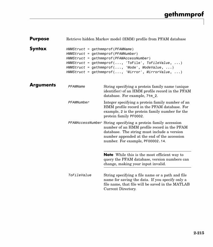
gethmmprof
Purpose Retrieve hidden Markov model (HMM) profile from PFAM database
Syntax HMMStruct = gethmmprof(PFAMName)HMMStruct = gethmmprof(PFAMNumber)HMMStruct = gethmmprof(PFAMAccessNumber)HMMStruct = gethmmprof(..., 'ToFile', ToFileValue, ...)HMMStruct = gethmmprof(..., 'Mode', ModeValue, ...)HMMStruct = gethmmprof(..., 'Mirror', MirrorValue, ...)
Arguments PFAMName String specifying a protein family name (uniqueidentifier) of an HMM profile record in the PFAMdatabase. For example, 7tm_2.
PFAMNumber Integer specifying a protein family number of anHMM profile record in the PFAM database. Forexample, 2 is the protein family number for theprotein family PF0002.
PFAMAccessNumber String specifying a protein family accessionnumber of an HMM profile record in the PFAMdatabase. The string must include a versionnumber appended at the end of the accessionnumber. For example, PF00002.14.
Note While this is the most efficient way toquery the PFAM database, version numbers canchange, making your input invalid.
ToFileValue String specifying a file name or a path and filename for saving the data. If you specify only afile name, that file will be saved in the MATLABCurrent Directory.
2-215

gethmmprof
ModeValue String that specifies the returned alignmentmode. Choices are:• ls — Default. Global alignment mode.
• fs — Local alignment mode.
MirrorValue String that specifies a Web database. Choices are:• Sanger (default)
• Janelia
ReturnValues
HMMStruct MATLAB structure containing informationretrieved from the PFAM database.
Description HMMStruct = gethmmprof(PFAMName) searches the PFAM database forthe record represented by PFAMName, a protein family name, retrievesthe HMM profile information, and stores it in HMMStruct, a MATLABstructure, with the following fields:
Field
Name
PfamAccessionNumber
ModelDescription
ModelLength
Alphabet
MatchEmission
InsertEmission
NullEmission
BeginX
MatchX
2-216
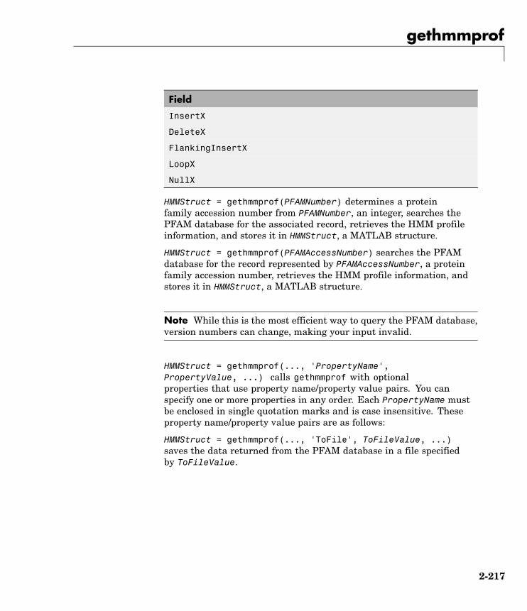
gethmmprof
Field
InsertX
DeleteX
FlankingInsertX
LoopX
NullX
HMMStruct = gethmmprof(PFAMNumber) determines a proteinfamily accession number from PFAMNumber, an integer, searches thePFAM database for the associated record, retrieves the HMM profileinformation, and stores it in HMMStruct, a MATLAB structure.
HMMStruct = gethmmprof(PFAMAccessNumber) searches the PFAMdatabase for the record represented by PFAMAccessNumber, a proteinfamily accession number, retrieves the HMM profile information, andstores it in HMMStruct, a MATLAB structure.
Note While this is the most efficient way to query the PFAM database,version numbers can change, making your input invalid.
HMMStruct = gethmmprof(..., 'PropertyName',PropertyValue, ...) calls gethmmprof with optionalproperties that use property name/property value pairs. You canspecify one or more properties in any order. Each PropertyName mustbe enclosed in single quotation marks and is case insensitive. Theseproperty name/property value pairs are as follows:
HMMStruct = gethmmprof(..., 'ToFile', ToFileValue, ...)saves the data returned from the PFAM database in a file specifiedby ToFileValue.
2-217

gethmmprof
Note You can read an HMM-formatted file back into MATLAB usingthe pfamhmmread function.
HMMStruct = gethmmprof(..., 'Mode', ModeValue, ...) specifiesthe returned alignment mode. Choices are:
• ls — Default. Global alignment mode.
• fs — Local alignment mode.
HMMStruct = gethmmprof(..., 'Mirror', MirrorValue, ...)specifies a Web database. Choices are:
• Sanger (default)
• Janelia
You can reach other mirror sites by passing the complete URL to thepfamhmmread function.
Note These mirror sites are maintained separately and may haveslight variations.
For more information about the PFAM database, see:
http://www.sanger.ac.uk/Software/Pfam/http://pfam.janelia.org/
Examples To retrieve a hidden Markov model (HMM) profile for the globalalignment of the 7-transmembrane receptor protein in the secretinfamily, enter either of the following:
hmm = gethmmprof(2)
2-218
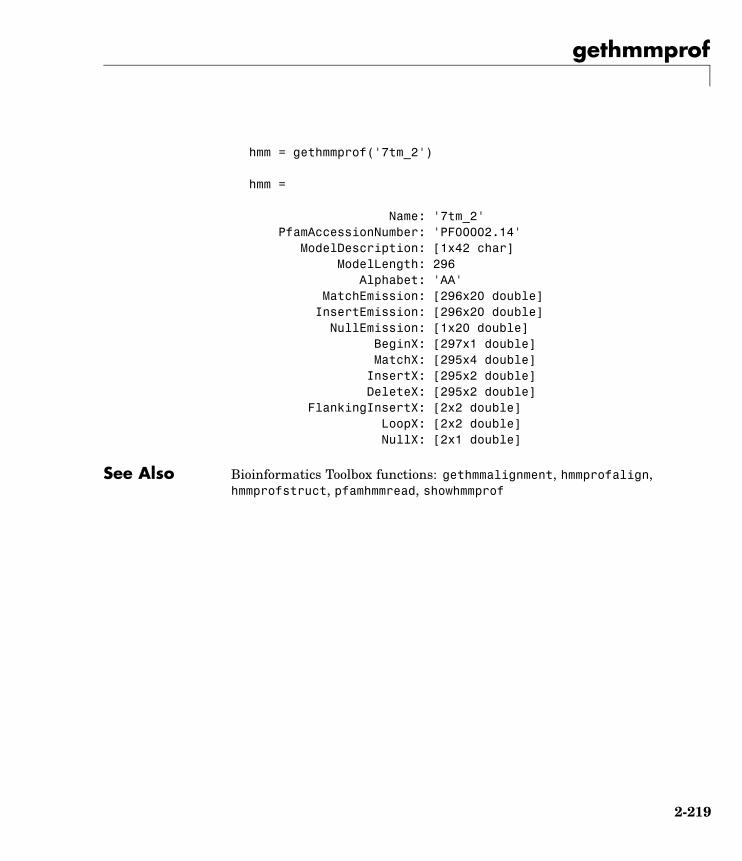
gethmmprof
hmm = gethmmprof('7tm_2')
hmm =
Name: '7tm_2'PfamAccessionNumber: 'PF00002.14'
ModelDescription: [1x42 char]ModelLength: 296
Alphabet: 'AA'MatchEmission: [296x20 double]
InsertEmission: [296x20 double]NullEmission: [1x20 double]
BeginX: [297x1 double]MatchX: [295x4 double]
InsertX: [295x2 double]DeleteX: [295x2 double]
FlankingInsertX: [2x2 double]LoopX: [2x2 double]NullX: [2x1 double]
See Also Bioinformatics Toolbox functions: gethmmalignment, hmmprofalign,hmmprofstruct, pfamhmmread, showhmmprof
2-219
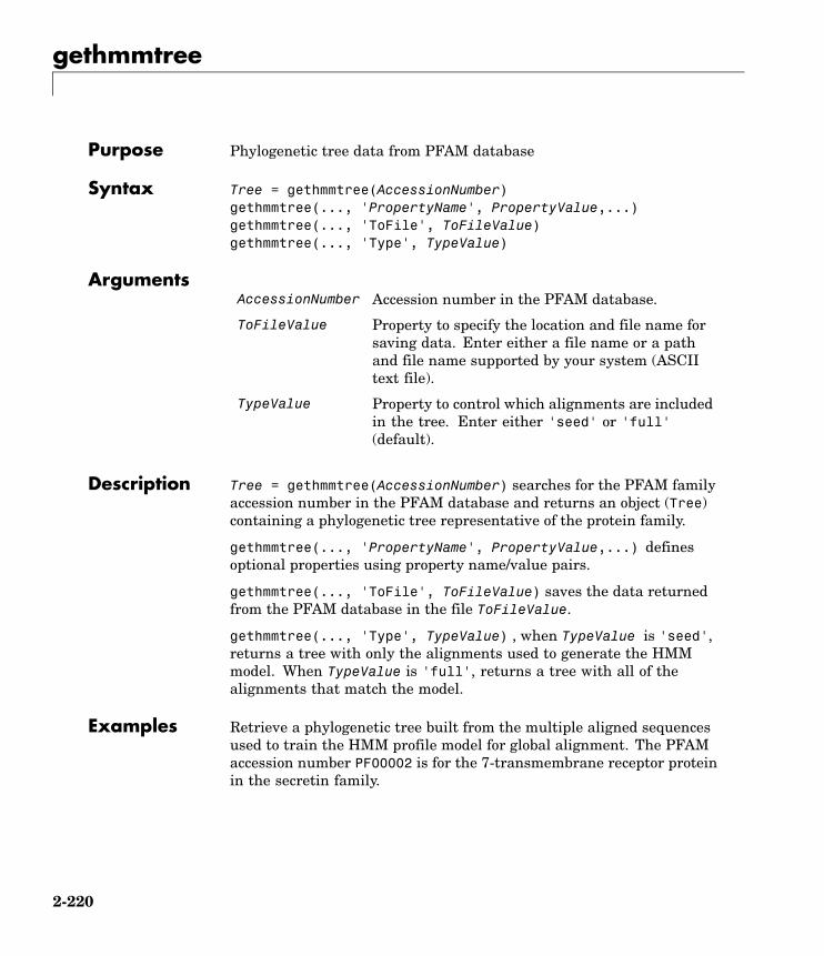
gethmmtree
Purpose Phylogenetic tree data from PFAM database
Syntax Tree = gethmmtree(AccessionNumber)gethmmtree(..., 'PropertyName', PropertyValue,...)gethmmtree(..., 'ToFile', ToFileValue)gethmmtree(..., 'Type', TypeValue)
ArgumentsAccessionNumber Accession number in the PFAM database.
ToFileValue Property to specify the location and file name forsaving data. Enter either a file name or a pathand file name supported by your system (ASCIItext file).
TypeValue Property to control which alignments are includedin the tree. Enter either 'seed' or 'full'(default).
Description Tree = gethmmtree(AccessionNumber) searches for the PFAM familyaccession number in the PFAM database and returns an object (Tree)containing a phylogenetic tree representative of the protein family.
gethmmtree(..., 'PropertyName', PropertyValue,...) definesoptional properties using property name/value pairs.
gethmmtree(..., 'ToFile', ToFileValue) saves the data returnedfrom the PFAM database in the file ToFileValue.
gethmmtree(..., 'Type', TypeValue) , when TypeValue is 'seed',returns a tree with only the alignments used to generate the HMMmodel. When TypeValue is 'full', returns a tree with all of thealignments that match the model.
Examples Retrieve a phylogenetic tree built from the multiple aligned sequencesused to train the HMM profile model for global alignment. The PFAMaccession number PF00002 is for the 7-transmembrane receptor proteinin the secretin family.
2-220
gethmmtree
tree = gethmmtree(2, 'type', 'seed')tree = gethmmtree('PF00002', 'type', 'seed')
See Also Bioinformatics Toolbox functions: gethmmalignment, phytreeread
2-221

getpdb
Purpose Retrieve protein structure data from Protein Data Bank (PDB) database
Syntax PDBStruct = getpdb(PDBid)PDBStruct = getpdb(PDBid, ...'ToFile', ToFileValue, ...)PDBStruct = getpdb(PDBid, ...'SequenceOnly',
SequenceOnlyValue, ...)
Arguments PDBid String specifying a unique identifier for aprotein structure record in the PDB database.
Note Each structure in the PDB database isrepresented by a four-character alphanumericidentifier. For example, 4hhb is the identifierfor hemoglobin.
ToFileValue String specifying a file name or a path and filename for saving the PDB-formatted data. If youspecify only a file name, that file will be savedin the MATLAB Current Directory.
Tip After you save the protein structure recordto a local PDB-formatted file, you can use thepdbread function to read the file into MATLABoffline or use the molviewer function to displayand manipulate a 3-D image of the structure.
SequenceOnlyValue Controls the return of the protein sequence only.Choices are true or false (default). If thereis one sequence, it is returned as a characterarray. If there are multiple sequences, they arereturned as a cell array.
2-222
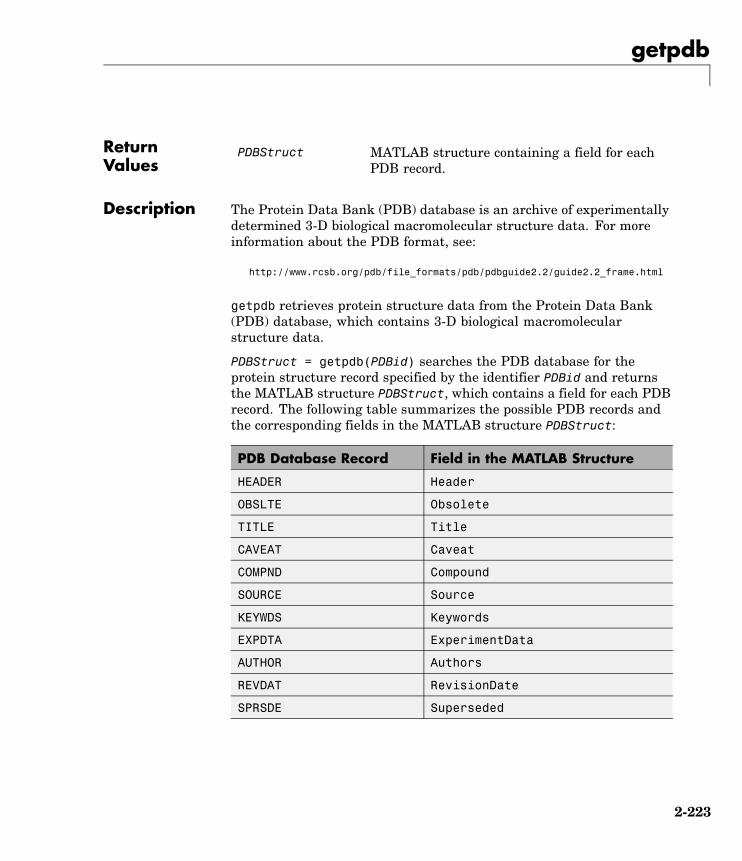
getpdb
ReturnValues
PDBStruct MATLAB structure containing a field for eachPDB record.
Description The Protein Data Bank (PDB) database is an archive of experimentallydetermined 3-D biological macromolecular structure data. For moreinformation about the PDB format, see:
http://www.rcsb.org/pdb/file_formats/pdb/pdbguide2.2/guide2.2_frame.html
getpdb retrieves protein structure data from the Protein Data Bank(PDB) database, which contains 3-D biological macromolecularstructure data.
PDBStruct = getpdb(PDBid) searches the PDB database for theprotein structure record specified by the identifier PDBid and returnsthe MATLAB structure PDBStruct, which contains a field for each PDBrecord. The following table summarizes the possible PDB records andthe corresponding fields in the MATLAB structure PDBStruct:
PDB Database Record Field in the MATLAB Structure
HEADER Header
OBSLTE Obsolete
TITLE Title
CAVEAT Caveat
COMPND Compound
SOURCE Source
KEYWDS Keywords
EXPDTA ExperimentData
AUTHOR Authors
REVDAT RevisionDate
SPRSDE Superseded
2-223

getpdb
PDB Database Record Field in the MATLAB Structure
JRNL Journal
REMARK 1 Remark1
REMARK N
Note N equals 2 through999.
Remarkn
Note n equals 2 through 999.
DBREF DBReferences
SEQADV SequenceConflicts
SEQRES Sequence
FTNOTE Footnote
MODRES ModifiedResidues
HET Heterogen
HETNAM HeterogenName
HETSYN HeterogenSynonym
FORMUL Formula
HELIX Helix
SHEET Sheet
TURN Turn
SSBOND SSBond
LINK Link
HYDBND HydrogenBond
SLTBRG SaltBridge
CISPEP CISPeptides
SITE Site
2-224

getpdb
PDB Database Record Field in the MATLAB Structure
CRYST1 Cryst1
ORIGXn OriginX
SCALEn Scale
MTRIXn Matrix
TVECT TranslationVector
MODEL Model
ATOM Atom
SIGATM AtomSD
ANISOU AnisotropicTemp
SIGUIJ AnisotropicTempSD
TER Terminal
HETATM HeterogenAtom
CONECT Connectivity
PDBStruct = getpdb(PDBid, ...'PropertyName',PropertyValue, ...) calls getpdb with optional propertiesthat use property name/property value pairs. You can specify one ormore properties in any order. Each PropertyName must be enclosedin single quotation marks and is case insensitive. These propertyname/property value pairs are as follows:
PDBStruct = getpdb(PDBid, ...'ToFile', ToFileValue, ...)saves the data returned from the database to a PDB-formatted file,ToFileValue.
Tip After you save the protein structure record to a local PDB-formattedfile, you can use the pdbread function to read the file into MATLABoffline or use the molviewer function to display and manipulate a 3-Dimage of the structure.
2-225

getpdb
PDBStruct = getpdb(PDBid, ...'SequenceOnly',SequenceOnlyValue, ...) controls the return of the proteinsequence only. Choices are true or false (default). If there is onesequence, it is returned as a character array. If there are multiplesequences, they are returned as a cell array.
The Sequence Field
The Sequence field is also a structure containing sequence informationin the following subfields:
• NumOfResidues
• ChainID
• ResidueNames — Contains the three-letter codes for the sequenceresidues.
• Sequence — Contains the single-letter codes for the sequenceresidues.
Note If the sequence has modified residues, then the ResidueNamessubfield might not correspond to the standard three-letter amino acidcodes. In this case, the Sequence subfield will contain the modifiedresidue code in the position corresponding to the modified residue. Themodified residue code is provided in the ModifiedResidues field.
The Model Field
The Model field is also a structure or an array of structures containingcoordinate information. If the MATLAB structure contains one model,the Model field is a structure containing coordinate information for thatmodel. If the MATLAB structure contains multiple models, the Modelfield is an array of structures containing coordinate information foreach model. The Model field contains the following subfields:
• Atom
• AtomSD
2-226

getpdb
• AnisotropicTemp
• AnisotropicTempSD
• Terminal
• HeterogenAtom
The Atom Field
The Atom field is also an array of structures containing the followingsubfields:
• AtomSerNo
• AtomName
• altLoc
• resName
• chainID
• resSeq
• iCode
• X
• Y
• Z
• occupancy
• tempFactor
• segID
• element
• charge
• AtomNameStruct — Contains three subfields: chemSymbol,remoteInd, and branch.
2-227

getpdb
Examples Retrieve the structure information for the electron transport (heme)protein that has a PDB identifier of 5CYT, read the information intoa MATLAB structure pdbstruct, and save the information to aPDB-formatted file electron_transport.pdb in the MATLAB CurrentDirectory.
pdbstruct = getpdb('5CYT', 'ToFile', 'electron_transport.pdb')
See Also Bioinformatics Toolbox functions: getembl, getgenbank, getgenpept,molviewer, pdbdistplot, pdbread, pdbwrite
2-228
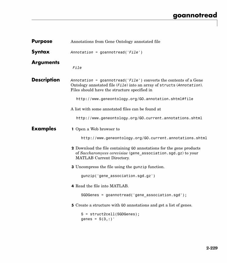
goannotread
Purpose Annotations from Gene Ontology annotated file
Syntax Annotation = goannotread('File')
ArgumentsFile
Description Annotation = goannotread('File') converts the contents of a GeneOntology annotated file (File) into an array of structs (Annotation).Files should have the structure specified in
http://www.geneontology.org/GO.annotation.shtml#file
A list with some annotated files can be found at
http://www.geneontology.org/GO.current.annotations.shtml
Examples 1 Open a Web browser to
http://www.geneontology.org/GO.current.annotations.shtml
2 Download the file containing GO annotations for the gene productsof Saccharomyces cerevisiae (gene_association.sgd.gz) to yourMATLAB Current Directory.
3 Uncompress the file using the gunzip function.
gunzip('gene_association.sgd.gz')
4 Read the file into MATLAB.
SGDGenes = goannotread('gene_association.sgd');
5 Create a structure with GO annotations and get a list of genes.
S = struct2cell(SGDGenes);genes = S(3,:)'
2-229
goannotread
See Also Bioinformatics Toolbox
• functions — geneont (object constructor), num2goid
• geneont object methods — getancestors, getdescendants,getmatrix, getrelatives
2-230

gonnet
Purpose Gonnet scoring matrix
Syntax gonnet
Description gonnet returns the Gonnet matrix.
The Gonnet matrix is the recommended mutation matrix for initiallyaligning protein sequences. Matrix elements are ten times thelogarithmic of the probability that the residues are aligned divided bythe probability that the residues are aligned by chance, and then matrixelements are normalized to 250 PAM units.
Expected score = -0.6152, Entropy = 1.6845 bits Lowest score = -8,Highest score = 14.2
Order:
A R N D C Q E G H I L K M F P S T W Y V B Z X *
References [1] Gaston H, Gonnet M, Cohen A, Benner S (1992), “Exhaustivematching of the entire protein sequence database”, Science,256:1443-1445.
See Also Bioinformatics Toolbox functions blosum, dayhoff, pam
2-231

gprread
Purpose Read microarray data from GenePix Results (GPR) file
Syntax GPRData = gprread('File')gprread(..., 'PropertyName', PropertyValue,...)gprread(..., 'CleanColNames', CleanColNamesValue)
ArgumentsFile GenePix Results formatted file (file extension
GPR). Enter a file name or a path and filename.
CleanColNamesValue Property to control creating column namesthat MATLAB can use as variable names.
Description GPRData = gprread('File') reads GenePix results data from Fileand creates a MATLAB structure (GPRData) with the following fields:
Field
Header
Data
Blocks
Columns
Rows
Names
IDs
ColumnNames
Indices
Shape
gprread(..., 'PropertyName', PropertyValue,...) definesoptional properties using property name/value pairs.
2-232

gprread
gprread(..., 'CleanColNames', CleanColNamesValue). A GPRfile may contain column names with spaces and some charactersthat MATLAB cannot use in MATLAB variable names. IfCleanColNamesValue is true, gprread returns names in the fieldColumnNames that are valid MATLAB variable names and names thatyou can use in functions. By default, CleanColNamesValue is falseand the field ColumnNames may contain characters that are invalid forMATLAB variable names.
The field Indices of the structure contains MATLAB indices that canbe used for plotting heat maps of the data.
For more details on the GPR format, see
http://www.moleculardevices.com/pages/software/gn_genepix_file_formats.html#gpr
http://www.moleculardevices.com/pages/software/gn_gpr_format_history.html
For a list of supported file format versions, see
http://www.moleculardevices.com/pages/software/gn_genepix_file_formats.html
GenePix is a registered trademark of Molecular Devices Corporation.
Examples % Read in a sample GPR file and plot the median foreground% intensity for the 635 nm channel.gprStruct = gprread('mouse_a1pd.gpr')maimage(gprStruct,'F635 Median');
% Alternatively you can create a similar plot using% more basic graphics commands.F635Median = magetfield(gprStruct,'F635 Median');imagesc(F635Median(gprStruct.Indices));colormap bonecolorbar;
2-233

gprread
See Also Bioinformatics Toolbox functions: affyread, agferead,celintensityread, galread, geosoftread, imageneread, magetfield,sptread
2-234

graphallshortestpaths
Purpose Find all shortest paths in graph
Syntax [dist] = graphallshortestpaths(G)[dist] = graphallshortestpaths(G, ...'Directed',DirectedValue, ...)[dist] = graphallshortestpaths(G, ...'Weights', WeightsValue,
...)
ArgumentsG N-by-N sparse matrix that represents a graph.
Nonzero entries in matrix G represent the weightsof the edges.
DirectedValue Property that indicates whether the graphis directed or undirected. Enter false for anundirected graph. This results in the upper triangleof the sparse matrix being ignored. Default is true.
WeightsValue Column vector that specifies custom weights forthe edges in matrix G. It must have one entryfor every nonzero value (edge) in matrix G. Theorder of the custom weights in the vector mustmatch the order of the nonzero values in matrix Gwhen it is traversed column-wise. This propertylets you use zero-valued weights. By default,graphallshortestpaths gets weight informationfrom the nonzero entries in matrix G.
DescriptionTip For introductory information on graph theory functions, see “GraphTheory Functions” in the Bioinformatics Toolbox documentation.
[dist] = graphallshortestpaths(G) finds the shortest pathsbetween every pair of nodes in the graph represented by matrix G, usingJohnson’s algorithm. Input G is an N-by-N sparse matrix that representsa graph. Nonzero entries in matrix G represent the weights of the edges.
2-235

graphallshortestpaths
Output dist is an N-by-N matrix where dist(S,T) is the distance ofthe shortest path from node S to node T. A 0 in this matrix indicates thesource node; an Inf is an unreachable node. The pred output is thepredecessor map of the winning paths.
Johnson’s algorithm has a time complexity of O(N*log(N)+N*E), whereN and E are the number of nodes and edges respectively.
[...] = graphallshortestpaths (G, 'PropertyName',PropertyValue, ...) calls graphallshortestpaths with optionalproperties that use property name/property value pairs. You canspecify one or more properties in any order. Each PropertyName mustbe enclosed in single quotes and is case insensitive. These propertyname/property value pairs are as follows:
[dist] = graphallshortestpaths(G, ...'Directed',DirectedValue, ...) indicates whether the graph is directedor undirected. Set DirectedValue to false for an undirected graph.This results in the upper triangle of the sparse matrix being ignored.Default is true.
[dist] = graphallshortestpaths(G, ...'Weights',WeightsValue, ...) lets you specify custom weights for theedges. WeightsValue is a column vector having one entry for everynonzero value (edge) in matrix G. The order of the custom weights in thevector must match the order of the nonzero values in matrix G when it istraversed column-wise. This property lets you use zero-valued weights.By default, graphallshortestpaths gets weight information from thenonzero entries in matrix G.
Examples Finding All Shortest Paths in a Directed Graph
1 Create and view a directed graph with 6 nodes and 11 edges.
W = [.41 .99 .51 .32 .15 .45 .38 .32 .36 .29 .21];DG = sparse([6 1 2 2 3 4 4 5 5 6 1],[2 6 3 5 4 1 6 3 4 3 5],W)
DG =
2-236
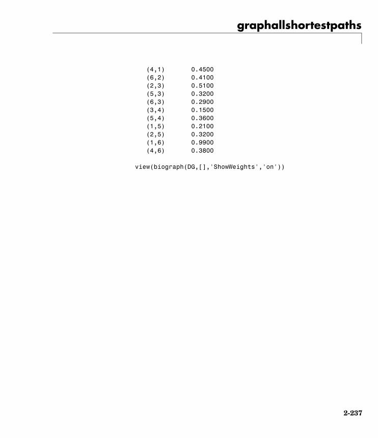
graphallshortestpaths
(4,1) 0.4500(6,2) 0.4100(2,3) 0.5100(5,3) 0.3200(6,3) 0.2900(3,4) 0.1500(5,4) 0.3600(1,5) 0.2100(2,5) 0.3200(1,6) 0.9900(4,6) 0.3800
view(biograph(DG,[],'ShowWeights','on'))
2-237
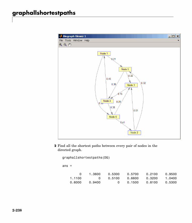
graphallshortestpaths
2 Find all the shortest paths between every pair of nodes in thedirected graph.
graphallshortestpaths(DG)
ans =
0 1.3600 0.5300 0.5700 0.2100 0.95001.1100 0 0.5100 0.6600 0.3200 1.04000.6000 0.9400 0 0.1500 0.8100 0.5300
2-238

graphallshortestpaths
0.4500 0.7900 0.6700 0 0.6600 0.38000.8100 1.1500 0.3200 0.3600 0 0.74000.8900 0.4100 0.2900 0.4400 0.7300 0
The resulting matrix shows the shortest path from node 1 (first row)to node 6 (sixth column) is 0.95. You can see this in the graph bytracing the path from node 1 to node 5 to node 4 to node 6 (0.21 +0.36 + 0.38 = 0.95).
Finding All Shortest Paths in an Undirected Graph
1 Create and view an undirected graph with 6 nodes and 11 edges.
UG = tril(DG + DG')
UG =
(4,1) 0.4500(5,1) 0.2100(6,1) 0.9900(3,2) 0.5100(5,2) 0.3200(6,2) 0.4100(4,3) 0.1500(5,3) 0.3200(6,3) 0.2900(5,4) 0.3600(6,4) 0.3800
view(biograph(UG,[],'ShowArrows','off','ShowWeights','on'))
2-239
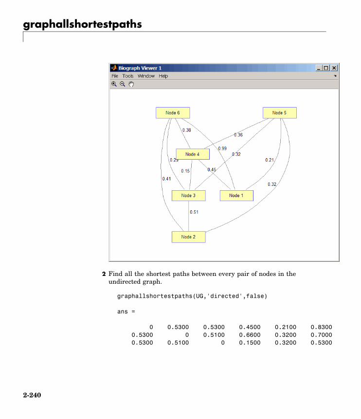
graphallshortestpaths
2 Find all the shortest paths between every pair of nodes in theundirected graph.
graphallshortestpaths(UG,'directed',false)
ans =
0 0.5300 0.5300 0.4500 0.2100 0.83000.5300 0 0.5100 0.6600 0.3200 0.70000.5300 0.5100 0 0.1500 0.3200 0.5300
2-240
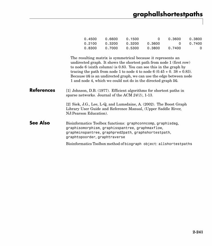
graphallshortestpaths
0.4500 0.6600 0.1500 0 0.3600 0.38000.2100 0.3200 0.3200 0.3600 0 0.74000.8300 0.7000 0.5300 0.3800 0.7400 0
The resulting matrix is symmetrical because it represents anundirected graph. It shows the shortest path from node 1 (first row)to node 6 (sixth column) is 0.83. You can see this in the graph bytracing the path from node 1 to node 4 to node 6 (0.45 + 0. 38 = 0.83).Because UG is an undirected graph, we can use the edge between node1 and node 4, which we could not do in the directed graph DG.
References [1] Johnson, D.B. (1977). Efficient algorithms for shortest paths insparse networks. Journal of the ACM 24(1), 1-13.
[2] Siek, J.G., Lee, L-Q, and Lumsdaine, A. (2002). The Boost GraphLibrary User Guide and Reference Manual, (Upper Saddle River,NJ:Pearson Education).
See Also Bioinformatics Toolbox functions: graphconncomp, graphisdag,graphisomorphism, graphisspantree, graphmaxflow,graphminspantree, graphpred2path, graphshortestpath,graphtopoorder, graphtraverse
Bioinformatics Toolbox method of biograph object: allshortestpaths
2-241

graphconncomp
Purpose Find strongly or weakly connected components in graph
Syntax [S, C] = graphconncomp(G)[S, C] = graphconncomp(G, ...'Directed', DirectedValue, ...)[S, C] = graphconncomp(G, ...'Weak', WeakValue, ...)
ArgumentsG N-by-N sparse matrix that represents a graph.
Nonzero entries in matrix G indicate the presenceof an edge.
DirectedValue Property that indicates whether the graph isdirected or undirected. Enter false for anundirected graph. This results in the uppertriangle of the sparse matrix being ignored.Default is true. A DFS-based algorithm computesthe connected components. Time complexity isO(N+E), where N and E are number of nodes andedges respectively.
WeakValue Property that indicates whether to find weaklyconnected components or strongly connectedcomponents. A weakly connected componentis a maximal group of nodes that are mutuallyreachable by violating the edge directions. SetWeakValue to true to find weakly connectedcomponents. Default is false, which finds stronglyconnected components. The state of this parameterhas no effect on undirected graphs because weaklyand strongly connected components are the samein undirected graphs. Time complexity is O(N+E),where N and E are number of nodes and edgesrespectively.
2-242

graphconncomp
DescriptionTip For introductory information on graph theory functions, see “GraphTheory Functions” in the Bioinformatics Toolbox documentation.
[S, C] = graphconncomp(G) finds the strongly connected componentsof the graph represented by matrix G using Tarjan’s algorithm. Astrongly connected component is a maximal group of nodes that aremutually reachable without violating the edge directions. Input G isan N-by-N sparse matrix that represents a graph. Nonzero entries inmatrix G indicate the presence of an edge.
The number of components found is returned in S, and C is a vectorindicating to which component each node belongs.
Tarjan’s algorithm has a time complexity of O(N+E), where N and E arethe number of nodes and edges respectively.
[S, C] = graphconncomp(G, ...'PropertyName',PropertyValue, ...) calls graphconncomp with optionalproperties that use property name/property value pairs. You canspecify one or more properties in any order. Each PropertyName mustbe enclosed in single quotes and is case insensitive. These propertyname/property value pairs are as follows:
[S, C] = graphconncomp(G, ...'Directed', DirectedValue, ...)indicates whether the graph is directed or undirected. SetdirectedValue to false for an undirected graph. This results in theupper triangle of the sparse matrix being ignored. Default is true.A DFS-based algorithm computes the connected components. Timecomplexity is O(N+E), where N and E are number of nodes and edgesrespectively.
[S, C] = graphconncomp(G, ...'Weak', WeakValue, ...) indicateswhether to find weakly connected components or strongly connectedcomponents. A weakly connected component is a maximal group ofnodes that are mutually reachable by violating the edge directions.Set WeakValue to true to find weakly connected components. Defaultis false, which finds strongly connected components. The state of this
2-243

graphconncomp
parameter has no effect on undirected graphs because weakly andstrongly connected components are the same in undirected graphs.Time complexity is O(N+E), where N and E are number of nodes andedges respectively.
Note By definition, a single node can be a strongly connectedcomponent.
Note A directed acyclic graph (DAG) cannot have any stronglyconnected components larger than one.
Examples 1 Create and view a directed graph with 10 nodes and 17 edges.
DG = sparse([1 1 1 2 2 3 3 4 5 6 7 7 8 9 9 9 9], ...[2 6 8 3 1 4 2 5 4 7 6 4 9 8 10 5 3],true,10,10)
DG =
(2,1) 1(1,2) 1(3,2) 1(2,3) 1(9,3) 1(3,4) 1(5,4) 1(7,4) 1(4,5) 1(9,5) 1(1,6) 1(7,6) 1(6,7) 1(1,8) 1(9,8) 1
2-244

graphconncomp
(8,9) 1(9,10) 1
h = view(biograph(DG));
2 Find the number of strongly connected components in the directedgraph and determine to which component each of the 10 nodesbelongs.
[S,C] = graphconncomp(DG)
2-245

graphconncomp
S =
4
C =
4 4 4 1 1 2 2 4 4 3
3 Color the nodes for each component with a different color.
colors = jet(S);for i = 1:numel(h.nodes)
h.Nodes(i).Color = colors(C(i),:);end
2-246

graphconncomp
References [1] Tarjan, R.E., (1972). Depth first search and linear graph algorithms.SIAM Journal on Computing 1(2), 146–160.
[2] Sedgewick, R., (2002). Algorithms in C++, Part 5 Graph Algorithms(Addison-Wesley).
[3] Siek, J.G., Lee, L-Q, and Lumsdaine, A. (2002). The Boost GraphLibrary User Guide and Reference Manual, (Upper Saddle River,NJ:Pearson Education).
2-247
graphconncomp
See Also Bioinformatics Toolbox functions: graphallshortestpaths,graphisdag, graphisomorphism, graphisspantree, graphmaxflow,graphminspantree, graphpred2path, graphshortestpath,graphtopoorder, graphtraverse
Bioinformatics Toolbox method of biograph object: conncomp
2-248
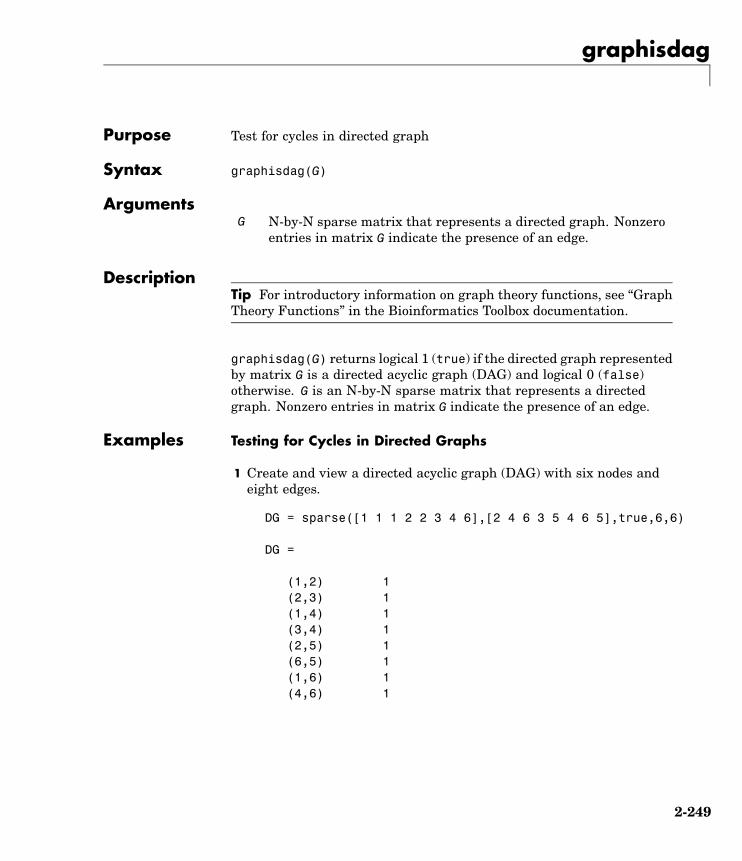
graphisdag
Purpose Test for cycles in directed graph
Syntax graphisdag(G)
ArgumentsG N-by-N sparse matrix that represents a directed graph. Nonzero
entries in matrix G indicate the presence of an edge.
DescriptionTip For introductory information on graph theory functions, see “GraphTheory Functions” in the Bioinformatics Toolbox documentation.
graphisdag(G) returns logical 1 (true) if the directed graph representedby matrix G is a directed acyclic graph (DAG) and logical 0 (false)otherwise. G is an N-by-N sparse matrix that represents a directedgraph. Nonzero entries in matrix G indicate the presence of an edge.
Examples Testing for Cycles in Directed Graphs
1 Create and view a directed acyclic graph (DAG) with six nodes andeight edges.
DG = sparse([1 1 1 2 2 3 4 6],[2 4 6 3 5 4 6 5],true,6,6)
DG =
(1,2) 1(2,3) 1(1,4) 1(3,4) 1(2,5) 1(6,5) 1(1,6) 1(4,6) 1
2-249

graphisdag
view(biograph(DG))
2 Test for cycles in the DAG.
graphisdag(DG)
ans =
1
2-250
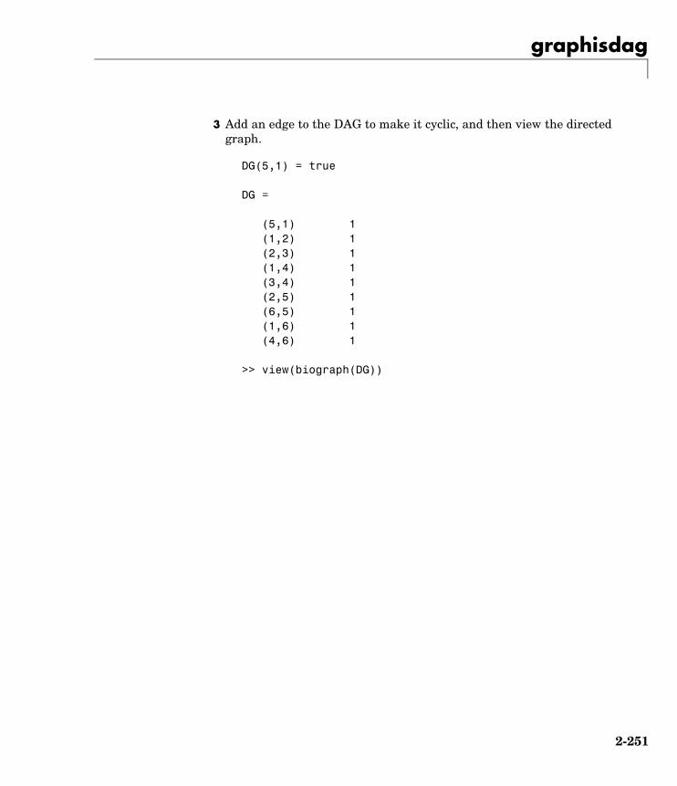
graphisdag
3 Add an edge to the DAG to make it cyclic, and then view the directedgraph.
DG(5,1) = true
DG =
(5,1) 1(1,2) 1(2,3) 1(1,4) 1(3,4) 1(2,5) 1(6,5) 1(1,6) 1(4,6) 1
>> view(biograph(DG))
2-251
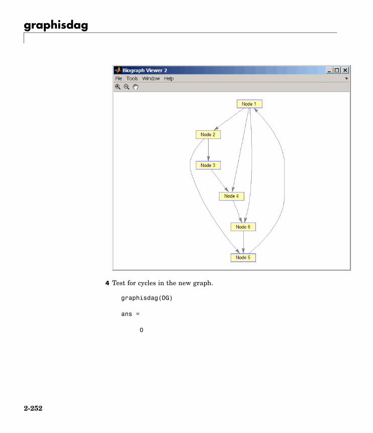
graphisdag
4 Test for cycles in the new graph.
graphisdag(DG)
ans =
0
2-252

graphisdag
Testing for Cycles in a Very Large Graph (Greater Than 20,000Nodes and 30,000 Edges)
1 Download the Gene Ontology database to a geneont object.
GO = geneont('live',true);
2 Convert the geneont object to a matrix.
CM = getmatrix(GO);
3 Test for cycles in the graph.
graphisdag(CM)
Creating a Random DAG
1 Create and view a random directed acyclic graph (DAG) with 15nodes and 20 edges.
g = sparse([],[],true,15,15);while nnz(g) < 20
edge = randsample(15*15,1); % get a random edgeg(edge) = true;g(edge) = graphisdag(g);
endview(biograph(g))
2 Test for cycles in the graph.
graphisdag(g)
References [1] Siek, J.G., Lee, L-Q, and Lumsdaine, A. (2002). The Boost GraphLibrary User Guide and Reference Manual, (Upper Saddle River,NJ:Pearson Education).
See Also Bioinformatics Toolbox functions: graphallshortestpaths,graphconncomp, graphisomorphism, graphisspantree, graphmaxflow,
2-253
graphisdag
graphminspantree, graphpred2path, graphshortestpath,graphtopoorder, graphtraverse
Bioinformatics Toolbox method of biograph object: isdag
2-254

graphisomorphism
Purpose Find isomorphism between two graphs
Syntax [Isomorphic, Map] = graphisomorphism(G1, G2)[Isomorphic, Map] = graphisomorphism(G1, G2,'Directed',
DirectedValue)
ArgumentsG1 N-by-N sparse matrix that represents a directed
or undirected graph. Nonzero entries in matrix G1indicate the presence of an edge.
G2 N-by-N sparse matrix that represents a directed orundirected graph. G2 must be the same (directed orundirected) as G1.
DirectedValue Property that indicates whether the graphs aredirected or undirected. Enter false when both G1and G2 are undirected graphs. In this case, theupper triangles of the sparse matrices G1 and G2are ignored. Default is true, meaning that bothgraphs are directed.
DescriptionTip For introductory information on graph theory functions, see “GraphTheory Functions” in the Bioinformatics Toolbox documentation.
[Isomorphic, Map] = graphisomorphism(G1, G2) returns logical 1(true) in Isomorphic if G1 and G2 are isomorphic graphs, and logical0 (false) otherwise. A graph isomorphism is a 1-to-1 mapping ofthe nodes in the graph G1 and the nodes in the graph G2 such thatadjacencies are preserved. G1 and G2 are both N-by-N sparse matricesthat represent directed or undirected graphs. Return value Isomorphicis Boolean. When Isomorphic is true, Map is a row vector containingthe node indices that map from G2 to G1. When Isomorphic is false,the worst-case time complexity is O(N!), where N is the number of nodes.
2-255

graphisomorphism
[Isomorphic, Map] = graphisomorphism(G1,G2,'Directed', DirectedValue) indicates whether the graphs aredirected or undirected. Set DirectedValue to false when both G1and G2 are undirected graphs. In this case, the upper triangles ofthe sparse matrices G1 and G2 are ignored. Default is true, meaningthat both graphs are directed.
Examples 1 Create and view a directed graph with 8 nodes and 11 edges.
m('ABCDEFGH') = [1 2 3 4 5 6 7 8];g1 = sparse(m('ABDCDCGEFFG'),m('BCBDGEEFHGH'),true,8,8)
g1 =
(1,2) 1(4,2) 1(2,3) 1(3,4) 1(3,5) 1(7,5) 1(5,6) 1(4,7) 1(6,7) 1(6,8) 1(7,8) 1
view(biograph(g1,'ABCDEFGH'))
2-256
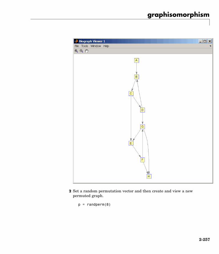
graphisomorphism
2 Set a random permutation vector and then create and view a newpermuted graph.
p = randperm(8)
2-257
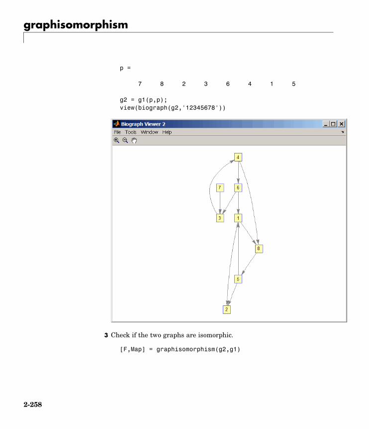
graphisomorphism
p =
7 8 2 3 6 4 1 5
g2 = g1(p,p);view(biograph(g2,'12345678'))
3 Check if the two graphs are isomorphic.
[F,Map] = graphisomorphism(g2,g1)
2-258
graphisomorphism
F =
1
Map =
7 8 2 3 6 4 1 5
Note that the Map row vector containing the node indices that mapfrom g2 to g1 is the same as the permutation vector you created instep 2.
4 Reverse the direction of the D-G edge in the first graph, and thencheck for isomorphism again.
g1(m('DG'),m('GD')) = g1(m('GD'),m('DG'));view(biograph(g1,'ABCDEFGH'))
2-259

graphisomorphism
[F,M] = graphisomorphism(g2,g1)
F =
0
M =
2-260

graphisomorphism
[]
5 Convert the graphs to undirected graphs, and then check forisomorphism.
[F,M] = graphisomorphism(g2+g2',g1+g1','directed',false)
F =
1
M =
7 8 2 3 6 4 1 5
References [1] Fortin, S. (1996). The Graph Isomorphism Problem. TechnicalReport, 96-20, Dept. of Computer Science, University of Alberta,Edomonton, Alberta, Canada.
[2] McKay, B.D. (1981). Practical Graph Isomorphism. CongressusNumerantium 30, 45-87.
[3] Siek, J.G., Lee, L-Q, and Lumsdaine, A. (2002). The Boost GraphLibrary User Guide and Reference Manual, (Upper Saddle River,NJ:Pearson Education).
See Also Bioinformatics Toolbox functions: graphallshortestpaths,graphconncomp, graphisdag, graphisspantree, graphmaxflow,graphminspantree, graphpred2path, graphshortestpath,graphtopoorder, graphtraverse
Bioinformatics Toolbox methods of biograph object: isomorphism
2-261

graphisspantree
Purpose Determine if tree is spanning tree
Syntax TF = graphisspantree(G)
ArgumentsG N-by-N sparse matrix whose lower triangle represents an
undirected graph. Nonzero entries in matrix G indicate thepresence of an edge.
DescriptionTip For introductory information on graph theory functions, see “GraphTheory Functions” in the Bioinformatics Toolbox documentation.
TF = graphisspantree(G) returns logical 1 (true) if G is a spanningtree, and logical 0 (false) otherwise. A spanning tree must touch all thenodes and must be acyclic. G is an N-by-N sparse matrix whose lowertriangle represents an undirected graph. Nonzero entries in matrix Gindicate the presence of an edge.
Examples 1 Create a phytree object from a phylogenetic tree file.
tr = phytreeread('pf00002.tree')Phylogenetic tree object with 33 leaves (32 branches)
2 Create a connection matrix from the phytree object.
[CM,labels,dist] = getmatrix(tr);
3 Determine if the connection matrix is a spanning tree.
graphisspantree(CM)
ans =
1
2-262

graphisspantree
4 Add an edge between the root and the first leaf in the connectionmatrix.
CM(end,1) = 1;
5 Determine if the modified connection matrix is a spanning tree.
graphisspantree(CM)
ans =
0
References [1] Siek, J.G., Lee, L-Q, and Lumsdaine, A. (2002). The Boost GraphLibrary User Guide and Reference Manual, (Upper Saddle River,NJ:Pearson Education).
See Also Bioinformatics Toolbox functions: graphallshortestpaths,graphconncomp, graphisdag, graphisomorphism, graphmaxflow,graphminspantree, graphpred2path, graphshortestpath,graphtopoorder, graphtraverse
Bioinformatics Toolbox methods of biograph object: isspantree
2-263
graphmaxflow
Purpose Calculate maximum flow and minimum cut in directed graph
Syntax [MaxFlow, FlowMatrix, Cut] = graphmaxflow(G, SNode, TNode)[...] = graphmaxflow(G, SNode, TNode, ...'Capacity',CapacityValue, ...)[...] = graphmaxflow(G, SNode, TNode, ...'Method', MethodValue,
...)
ArgumentsG N-by-N sparse matrix that represents a directed
graph. Nonzero entries in matrix G represent thecapacities of the edges.
SNode Node in G.
TNode Node in G.
CapacityValue Column vector that specifies custom capacities forthe edges in matrix G. It must have one entry forevery nonzero value (edge) in matrix G. The order ofthe custom capacities in the vector must match theorder of the nonzero values in matrix G when it istraversed column-wise. By default, graphmaxflowgets capacity information from the nonzero entriesin matrix G.
MethodValue String that specifies the algorithm used to find theminimal spanning tree (MST). Choices are:• 'Edmonds' — Uses the Edmonds and Karp
algorithm, the implementation of which is basedon a variation called the labeling algorithm. Timecomplexity is O(N*E^2), where N and E are thenumber of nodes and edges respectively.
• 'Goldberg' — Default algorithm. Uses theGoldberg algorithm, which uses the genericmethod known as preflow-push. Time complexityis O(N^2*sqrt(E)), where N and E are thenumber of nodes and edges respectively.
2-264
graphmaxflow
DescriptionTip For introductory information on graph theory functions, see “GraphTheory Functions” in the Bioinformatics Toolbox documentation.
[MaxFlow, FlowMatrix, Cut] = graphmaxflow(G, SNode, TNode)calculates the maximum flow of directed graph G from node SNode tonode TNode. Input G is an N-by-N sparse matrix that represents adirected graph. Nonzero entries in matrix G represent the capacities ofthe edges. Output MaxFlow is the maximum flow, and FlowMatrix is asparse matrix with all the flow values for every edge. FlowMatrix(X,Y)is the flow from node X to node Y. Output Cut is a logical row vectorindicating the nodes connected to SNode after calculating the minimumcut between SNode and TNode. If several solutions to the minimum cutproblem exist, then Cut is a matrix.
[...] = graphmaxflow(G, SNode, TNode, ...'PropertyName',PropertyValue, ...) calls graphmaxflow with optional propertiesthat use property name/property value pairs. You can specify one ormore properties in any order. Each PropertyName must be enclosed insingle quotes and is case insensitive. These property name/propertyvalue pairs are as follows:
[...] = graphmaxflow(G, SNode, TNode, ...'Capacity',CapacityValue, ...) lets you specify custom capacities for the edges.CapacityValue is a column vector having one entry for every nonzerovalue (edge) in matrix G. The order of the custom capacities in thevector must match the order of the nonzero values in matrix G whenit is traversed column-wise. By default, graphmaxflow gets capacityinformation from the nonzero entries in matrix G.
[...] = graphmaxflow(G, SNode, TNode, ...'Method',MethodValue, ...) lets you specify the algorithm used to find theminimal spanning tree (MST). Choices are:
• 'Edmonds' — Uses the Edmonds and Karp algorithm, theimplementation of which is based on a variation called the labeling
2-265

graphmaxflow
algorithm. Time complexity is O(N*E^2), where N and E are thenumber of nodes and edges respectively.
• 'Goldberg' — Default algorithm. Uses the Goldberg algorithm,which uses the generic method known as preflow-push. Timecomplexity is O(N^2*sqrt(E)), where N and E are the number ofnodes and edges respectively.
Examples 1 Create a directed graph with six nodes and eight edges.
cm = sparse([1 1 2 2 3 3 4 5],[2 3 4 5 4 5 6 6],...[2 3 3 1 1 1 2 3],6,6)
cm =
(1,2) 2(1,3) 3(2,4) 3(3,4) 1(2,5) 1(3,5) 1(4,6) 2(5,6) 3
2 Calculate the maximum flow in the graph from node 1 to node 6.
[M,F,K] = graphmaxflow(cm,1,6)
M =
4
F =
(1,2) 2(1,3) 2(2,4) 1(3,4) 1
2-266

graphmaxflow
(2,5) 1(3,5) 1(4,6) 2(5,6) 2
K =
1 1 1 1 0 01 0 1 0 0 0
Notice that K is a two-row matrix because there are two possiblesolutions to the minimum cut problem.
3 View the graph with the original capacities.
h = view(biograph(cm,[],'ShowWeights','on'))
2-267
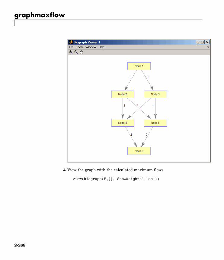
graphmaxflow
4 View the graph with the calculated maximum flows.
view(biograph(F,[],'ShowWeights','on'))
2-268

graphmaxflow
5 Show one solution to the minimum cut problem in the original graph.
set(h.Nodes(K(1,:)),'Color',[1 0 0])
2-269
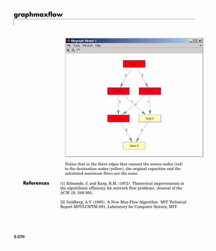
graphmaxflow
Notice that in the three edges that connect the source nodes (red)to the destination nodes (yellow), the original capacities and thecalculated maximum flows are the same.
References [1] Edmonds, J. and Karp, R.M. (1972). Theoretical improvements inthe algorithmic efficiency for network flow problems. Journal of theACM 19, 248-264.
[2] Goldberg, A.V. (1985). A New Max-Flow Algorithm. MIT TechnicalReport MIT/LCS/TM-291, Laboratory for Computer Science, MIT.
2-270

graphmaxflow
[3] Siek, J.G., Lee, L-Q, and Lumsdaine, A. (2002). The Boost GraphLibrary User Guide and Reference Manual, (Upper Saddle River,NJ:Pearson Education).
See Also Bioinformatics Toolbox functions: graphallshortestpaths,graphconncomp, graphisdag, graphisomorphism, graphisspantree,graphminspantree, graphpred2path, graphshortestpath,graphtopoorder, graphtraverse
Bioinformatics Toolbox method of biograph object: maxflow
2-271
graphminspantree
Purpose Find minimal spanning tree in graph
Syntax [Tree, pred] = graphminspantree(G)[Tree, pred] = graphminspantree(G, R)[Tree, pred] = graphminspantree(..., 'Method', MethodValue, ...)[Tree, pred] = graphminspantree(..., 'Weights', WeightsValue,
...)
ArgumentsG N-by-N sparse matrix that represents an undirected graph.
Nonzero entries in matrix G represent the weights of the edges.
R Scalar between 1 and the number of nodes.
DescriptionTip For introductory information on graph theory functions, see “GraphTheory Functions” in the Bioinformatics Toolbox documentation.
[Tree, pred] = graphminspantree(G) finds an acyclic subset of edgesthat connects all the nodes in the undirected graph G and for which thetotal weight is minimized. Weights of the edges are all nonzero entriesin the lower triangle of the N-by-N sparse matrix G. Output Tree is aspanning tree represented by a sparse matrix. Output pred is a vectorcontaining the predecessor nodes of the minimal spanning tree (MST),with the root node indicated by 0. The root node defaults to the firstnode in the largest connected component. This computation requiresan extra call to the graphconncomp function.
[Tree, pred] = graphminspantree(G, R) sets the root of theminimal spanning tree to node R.
[Tree,pred] = graphminspantree(..., 'PropertyName', PropertyValue, ...)calls graphminspantree with optional properties that use propertyname/property value pairs. You can specify one or more properties inany order. Each PropertyName must be enclosed in single quotes
2-272

graphminspantree
and is case insensitive. These property name/property valuepairs are as follows:
[Tree, pred] = graphminspantree(..., 'Method', MethodValue, ...)lets you specify the algorithm used to find the minimal spanning tree(MST). Choices are:
• 'Kruskal' — Grows the minimal spanning tree (MST) one edge at atime by finding an edge that connects two trees in a spreading forestof growing MSTs. Time complexity is O(E+X*log(N)), where X is thenumber of edges no longer than the longest edge in the MST, and Nand E are the number of nodes and edges respectively.
• 'Prim' — Default algorithm. Grows the minimal spanning tree(MST) one edge at a time by adding a minimal edge that connectsa node in the growing MST with any other node. Time complexityis O(E*log(N)), where N and E are the number of nodes and edgesrespectively.
Note When the graph is unconnected, Prim’s algorithm returns onlythe tree that contains R, while Kruskal’s algorithm returns an MSTfor every component.
[Tree, pred] = graphminspantree(..., 'Weights',WeightsValue, ...) lets you specify custom weights for theedges. WeightsValue is a column vector having one entry for everynonzero value (edge) in matrix G. The order of the custom weights in thevector must match the order of the nonzero values in matrix G when itis traversed column-wise. By default, graphminspantree gets weightinformation from the nonzero entries in matrix G.
Examples 1 Create and view an undirected graph with 6 nodes and 11 edges.
W = [.41 .29 .51 .32 .50 .45 .38 .32 .36 .29 .21];DG = sparse([1 1 2 2 3 4 4 5 5 6 6],[2 6 3 5 4 1 6 3 4 2 5],W);
2-273

graphminspantree
UG = tril(DG + DG')
UG =
(2,1) 0.4100(4,1) 0.4500(6,1) 0.2900(3,2) 0.5100(5,2) 0.3200(6,2) 0.2900(4,3) 0.5000(5,3) 0.3200(5,4) 0.3600(6,4) 0.3800(6,5) 0.2100
view(biograph(UG,[],'ShowArrows','off','ShowWeights','on'))
2-274
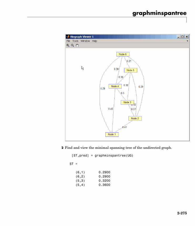
graphminspantree
2 Find and view the minimal spanning tree of the undirected graph.
[ST,pred] = graphminspantree(UG)
ST =
(6,1) 0.2900(6,2) 0.2900(5,3) 0.3200(5,4) 0.3600
2-275

graphminspantree
(6,5) 0.2100
pred =
0 6 5 5 6 1
view(biograph(ST,[],'ShowArrows','off','ShowWeights','on'))
2-276

graphminspantree
References [1] Kruskal, J.B. (1956). On the Shortest Spanning Subtree of a Graphand the Traveling Salesman Problem. Proceedings of the AmericanMathematical Society 7, 48-50.
[2] Prim, R. (1957). Shortest Connection Networks and SomeGeneralizations. Bell System Technical Journal 36, 1389-1401.
[3] Siek, J.G. Lee, L-Q, and Lumsdaine, A. (2002). The Boost GraphLibrary User Guide and Reference Manual, (Upper Saddle River,NJ:Pearson Education).
See Also Bioinformatics Toolbox functions: graphallshortestpaths,graphconncomp, graphisdag, graphisomorphism, graphisspantree,graphmaxflow, graphpred2path, graphshortestpath,graphtopoorder, graphtraverse
Bioinformatics Toolbox method of biograph object: minspantree
2-277
graphpred2path
Purpose Convert predecessor indices to paths
Syntax path = graphpred2path(pred, D)
Argumentspred Row vector or matrix of predecessor node indices. The value
of the root (or source) node in pred must be 0.
D Destination node in pred.
DescriptionTip For introductory information on graph theory functions, see “GraphTheory Functions” in the Bioinformatics Toolbox documentation.
path = graphpred2path(pred, D) traces back a path by following thepredecessor list in pred starting at destination node D.
The value of the root (or source) node in pred must be 0. If a NaN isfound when following the predecessor nodes, graphpred2path returnsan empty path.
If pred is a ... And D isa ...
Then path is a ...
scalar row vector listing the nodes from theroot (or source) to D.
row vector ofpredecessornode indices row vector row cell array with every column
containing the path to the destinationfor every element in D.
2-278
graphpred2path
If pred is a ... And D isa ...
Then path is a ...
scalar column cell array with every rowcontaining the path for every row inpred.
matrix
row vector matrix cell array with every rowcontaining the paths for the respectiverow in pred, and every columncontaining the paths to the respectivedestination in D.
Note If D is omitted, the paths to all the destinations are calculated forevery predecessor listed in pred.
Examples 1 Create a phytree object from the phylogenetic tree file for theGLR_HUMAN protein.
tr = phytreeread('pf00002.tree')Phylogenetic tree object with 33 leaves (32 branches)
2 View the phytree object.
view(tr)
2-279

graphpred2path
3 From the phytree object, create a connection matrix to represent thephylogenetic tree.
[CM,labels,dist] = getmatrix(tr);
4 Find the nodes from the root to one leaf in the phylogenetic treecreated from the phylogenetic tree file for the GLR_HUMAN protein.
root_loc = size(CM,1)
root_loc =
2-280

graphpred2path
65
glr_loc = strmatch('GLR',labels)
glr_loc =
28
[T,PRED]=graphminspantree(CM,root_loc);PATH = graphpred2path(PRED,glr_loc)
PATH =
65 64 53 52 46 45 44 43 28
References [1] Siek, J.G., Lee, L-Q, and Lumsdaine, A. (2002). The Boost GraphLibrary User Guide and Reference Manual, (Upper Saddle River,NJ:Pearson Education).
See Also Bioinformatics Toolbox functions: graphallshortestpaths,graphconncomp, graphisdag, graphisomorphism, graphisspantree,graphmaxflow, graphminspantree, graphshortestpath,graphtopoorder, graphtraverse
2-281
graphshortestpath
Purpose Solve shortest path problem in graph
Syntax [dist, path, pred] = graphshortestpath(G, S)[dist, path, pred] = graphshortestpath(G, S, T)[...] = graphshortestpath(..., 'Directed', DirectedValue, ...)[...] = graphshortestpath(..., 'Method', MethodValue, ...)[...] = graphshortestpath(..., 'Weights', WeightsValue, ...)
ArgumentsG N-by-N sparse matrix that represents a graph.
Nonzero entries in matrix G represent the weightsof the edges.
S Node in G.
T Node in G.
DirectedValue Property that indicates whether the graphis directed or undirected. Enter false for anundirected graph. This results in the upper triangleof the sparse matrix being ignored. Default is true.
2-282

graphshortestpath
MethodValue String that specifies the algorithm used to find theshortest path. Choices are:• 'Bellman-Ford' — Assumes weights of the
edges to be nonzero entries in sparse matrix G.Time complexity is O(N*E), where N and E arethe number of nodes and edges respectively.
• 'BFS' — Breadth-first search. Assumes allweights to be equal, and nonzero entries insparse matrix G to represent edges. Timecomplexity is O(N+E), where N and E are thenumber of nodes and edges respectively.
• 'Acyclic' — Assumes G to be a directed acyclicgraph and that weights of the edges are nonzeroentries in sparse matrix G. Time complexity isO(N+E), where N and E are the number of nodesand edges respectively.
• 'Dijkstra' — Default algorithm. Assumesweights of the edges to be positive valuesin sparse matrix G. Time complexity isO(log(N)*E), where N and E are the number ofnodes and edges respectively.
WeightsValue Column vector that specifies custom weights forthe edges in matrix G. It must have one entryfor every nonzero value (edge) in matrix G. Theorder of the custom weights in the vector mustmatch the order of the nonzero values in matrix Gwhen it is traversed column-wise. This propertylets you use zero-valued weights. By default,graphshortestpaths gets weight information fromthe nonzero entries in matrix G.
2-283

graphshortestpath
DescriptionTip For introductory information on graph theory functions, see “GraphTheory Functions” in the Bioinformatics Toolbox documentation.
[dist, path, pred] = graphshortestpath(G, S) determines thesingle-source shortest paths from node S to all other nodes in thegraph represented by matrix G. Input G is an N-by-N sparse matrixthat represents a graph. Nonzero entries in matrix G represent theweights of the edges. dist are the N distances from the source to everynode (using Infs for nonreachable nodes and 0 for the source node).path contains the winning paths to every node. pred contains thepredecessor nodes of the winning paths.
[dist, path, pred] = graphshortestpath(G, S, T) determinesthe single source-single destination shortest path from node S to node T.
[...] = graphshortestpath(..., 'PropertyName',PropertyValue, ...) calls graphshortestpath with optionalproperties that use property name/property value pairs. You canspecify one or more properties in any order. Each PropertyName mustbe enclosed in single quotes and is case insensitive. These propertyname/property value pairs are as follows:
[...] = graphshortestpath(..., 'Directed', DirectedValue, ...)indicates whether the graph is directed or undirected. SetDirectedValue to false for an undirected graph. This results in theupper triangle of the sparse matrix being ignored. Default is true.
[...] = graphshortestpath(..., 'Method', MethodValue, ...) letsyou specify the algorithm used to find the shortest path. Choices are:
• 'Bellman-Ford' — Assumes weights of the edges to be nonzeroentries in sparse matrix G. Time complexity is O(N*E), where N and Eare the number of nodes and edges respectively.
• 'BFS' — Breadth-first search. Assumes all weights to be equal,and nonzero entries in sparse matrix G to represent edges. Time
2-284

graphshortestpath
complexity is O(N+E), where N and E are the number of nodes andedges respectively.
• 'Acyclic' — Assumes G to be a directed acyclic graph and thatweights of the edges are nonzero entries in sparse matrix G. Timecomplexity is O(N+E), where N and E are the number of nodes andedges respectively.
• 'Dijkstra' — Default algorithm. Assumes weights of the edges to bepositive values in sparse matrix G. Time complexity is O(log(N)*E),where N and E are the number of nodes and edges respectively.
[...] = graphshortestpath(..., 'Weights', WeightsValue, ...)lets you specify custom weights for the edges. WeightsValue is acolumn vector having one entry for every nonzero value (edge) inmatrix G. The order of the custom weights in the vector must matchthe order of the nonzero values in matrix G when it is traversedcolumn-wise. This property lets you use zero-valued weights. Bydefault, graphshortestpath gets weight information from the nonzeroentries in matrix G.
Examples Finding the Shortest Path in a Directed Graph
1 Create and view a directed graph with 6 nodes and 11 edges.
W = [.41 .99 .51 .32 .15 .45 .38 .32 .36 .29 .21];DG = sparse([6 1 2 2 3 4 4 5 5 6 1],[2 6 3 5 4 1 6 3 4 3 5],W)
DG =
(4,1) 0.4500(6,2) 0.4100(2,3) 0.5100(5,3) 0.3200(6,3) 0.2900(3,4) 0.1500(5,4) 0.3600(1,5) 0.2100
2-285

graphshortestpath
(2,5) 0.3200(1,6) 0.9900(4,6) 0.3800
h = view(biograph(DG,[],'ShowWeights','on'))Biograph object with 6 nodes and 11 edges.
2 Find the shortest path in the graph from node 1 to node 6.
[dist,path,pred] = graphshortestpath(DG,1,6)
2-286

graphshortestpath
dist =
0.9500
path =
1 5 4 6
pred =
0 6 5 5 1 4
3 Mark the nodes and edges of the shortest path by coloring them redand increasing the line width.
set(h.Nodes(path),'Color',[1 0.4 0.4])edges = getedgesbynodeid(h,get(h.Nodes(path),'ID'));set(edges,'LineColor',[1 0 0])set(edges,'LineWidth',1.5)
2-287
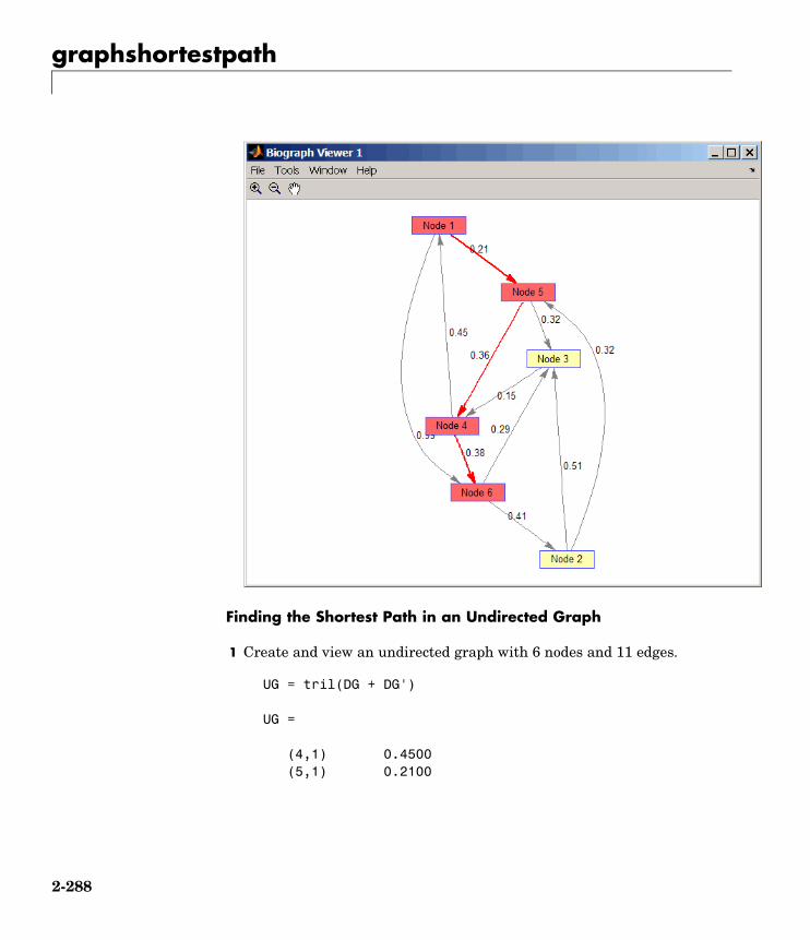
graphshortestpath
Finding the Shortest Path in an Undirected Graph
1 Create and view an undirected graph with 6 nodes and 11 edges.
UG = tril(DG + DG')
UG =
(4,1) 0.4500(5,1) 0.2100
2-288

graphshortestpath
(6,1) 0.9900(3,2) 0.5100(5,2) 0.3200(6,2) 0.4100(4,3) 0.1500(5,3) 0.3200(6,3) 0.2900(5,4) 0.3600(6,4) 0.3800
h = view(biograph(UG,[],'ShowArrows','off','ShowWeights','on'))Biograph object with 6 nodes and 11 edges.
2-289

graphshortestpath
2 Find the shortest path in the graph from node 1 to node 6.
[dist,path,pred] = graphshortestpath(UG,1,6,'directed',false)
dist =
0.8200
path =
2-290

graphshortestpath
1 5 3 6
pred =
0 5 5 1 1 3
3 Mark the nodes and edges of the shortest path by coloring them redand increasing the line width.
set(h.Nodes(path),'Color',[1 0.4 0.4])fowEdges = getedgesbynodeid(h,get(h.Nodes(path),'ID'));revEdges = getedgesbynodeid(h,get(h.Nodes(fliplr(path)),'ID'));edges = [fowEdges;revEdges];set(edges,'LineColor',[1 0 0])set(edges,'LineWidth',1.5)
2-291

graphshortestpath
References [1] Dijkstra, E.W. (1959). A note on two problems in connexion withgraphs. Numerische Mathematik 1, 269-271.
[2] Bellman, R. (1958). On a Routing Problem. Quarterly of AppliedMathematics 16(1), 87-90.
[3] Siek, J.G., Lee, L-Q, and Lumsdaine, A. (2002). The Boost GraphLibrary User Guide and Reference Manual, (Upper Saddle River,NJ:Pearson Education).
2-292
graphshortestpath
See Also Bioinformatics Toolbox functions: graphallshortestpaths,graphconncomp, graphisdag, graphisomorphism, graphisspantree,graphmaxflow, graphminspantree, graphpred2path, graphtopoorder,graphtraverse
Bioinformatics Toolbox method of biograph object: shortestpath
2-293

graphtopoorder
Purpose Perform topological sort of directed acyclic graph
Syntax order = graphtopoorder(G)
ArgumentsG N-by-N sparse matrix that represents a directed acyclic graph.
Nonzero entries in matrix G indicate the presence of an edge.
DescriptionTip For introductory information on graph theory functions, see “GraphTheory Functions” in the Bioinformatics Toolbox documentation.
order = graphtopoorder(G) returns an index vector with the order ofthe nodes sorted topologically. In topological order, an edge can existbetween a source node u and a destination node v, if and only if uappears before v in the vector order. G is an N-by-N sparse matrix thatrepresents a directed acyclic graph (DAG). Nonzero entries in matrix Gindicate the presence of an edge.
Examples 1 Create and view a directed acyclic graph (DAG) with six nodes andeight edges.
DG = sparse([6 6 6 2 2 3 5 1],[2 5 1 3 4 5 1 4],true,6,6)
DG =
(5,1) 1(6,1) 1(6,2) 1(2,3) 1(1,4) 1(2,4) 1(3,5) 1(6,5) 1
2-294
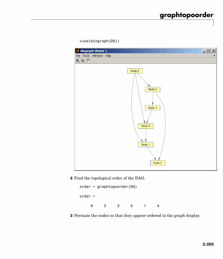
graphtopoorder
view(biograph(DG))
2 Find the topological order of the DAG.
order = graphtopoorder(DG)
order =
6 2 3 5 1 4
3 Permute the nodes so that they appear ordered in the graph display.
2-295

graphtopoorder
DG = DG(order,order)
DG =
(1,2) 1(2,3) 1(1,4) 1(3,4) 1(1,5) 1(4,5) 1(2,6) 1(5,6) 1
view(biograph(DG))
2-296

graphtopoorder
References [1] Siek, J.G., Lee, L-Q, and Lumsdaine, A. (2002). The Boost GraphLibrary User Guide and Reference Manual, (Upper Saddle River,NJ:Pearson Education).
See Also Bioinformatics Toolbox functions: graphallshortestpaths,graphconncomp, graphisdag, graphisomorphism, graphisspantree,graphmaxflow, graphminspantree, graphpred2path,graphshortestpath, graphtraverse
Bioinformatics Toolbox method of biograph object: topoorder
2-297

graphtraverse
Purpose Traverse graph by following adjacent nodes
Syntax [disc, pred, closed] = graphtraverse(G, S)[...] = graphtraverse(G, S, ...'Depth', DepthValue, ...)[...] = graphtraverse(G, S, ...'Directed', DirectedValue, ...)[...] = graphtraverse(G, S, ...'Method', MethodValue, ...)
ArgumentsG N-by-N sparse matrix that represents a directed
graph. Nonzero entries in matrix G indicate thepresence of an edge.
S Integer that indicates the source node in graph G.
DepthValue Integer that indicates a node in graph G thatspecifies the depth of the search. Default is Inf(infinity).
DirectedValue Property that indicates whether graph G is directedor undirected. Enter false for an undirectedgraph. This results in the upper triangle of thesparse matrix being ignored. Default is true.
MethodValue String that specifies the algorithm used to traversethe graph. Choices are:• 'BFS' — Breadth-first search. Time complexity
is O(N+E), where N and E are number of nodesand edges respectively.
• 'DFS' — Default algorithm. Depth-first search.Time complexity is O(N+E), where N and E arenumber of nodes and edges respectively.
DescriptionTip For introductory information on graph theory functions, see “GraphTheory Functions” in the Bioinformatics Toolbox documentation.
2-298

graphtraverse
[disc, pred, closed] = graphtraverse(G, S) traverses graph Gstarting from the node indicated by integer S. G is an N-by-N sparsematrix that represents a directed graph. Nonzero entries in matrix Gindicate the presence of an edge. disc is a vector of node indices inthe order in which they are discovered. pred is a vector of predecessornode indices (listed in the order of the node indices) of the resultingspanning tree. closed is a vector of node indices in the order in whichthey are closed.
[...] = graphtraverse(G, S, ...'PropertyName',PropertyValue, ...) calls graphtraverse with optional propertiesthat use property name/property value pairs. You can specify one ormore properties in any order. Each PropertyName must be enclosed insingle quotes and is case insensitive. These property name/propertyvalue pairs are as follows:
[...] = graphtraverse(G, S, ...'Depth', DepthValue, ...)specifies the depth of the search. DepthValue is an integer indicating anode in graph G. Default is Inf (infinity).
[...] = graphtraverse(G, S, ...'Directed', DirectedValue, ...)indicates whether the graph is directed or undirected. SetDirectedValue to false for an undirected graph. This results in theupper triangle of the sparse matrix being ignored. Default is true.
[...] = graphtraverse(G, S, ...'Method', MethodValue, ...) letsyou specify the algorithm used to traverse the graph. Choices are:
• 'BFS' — Breadth-first search. Time complexity is O(N+E), where Nand E are number of nodes and edges respectively.
• 'DFS' — Default algorithm. Depth-first search. Time complexity isO(N+E), where N and E are number of nodes and edges respectively.
Examples 1 Create a directed graph with 10 nodes and 12 edges.
DG = sparse([1 2 3 4 5 5 5 6 7 8 8 9],...[2 4 1 5 3 6 7 9 8 1 10 2],true,10,10)
2-299
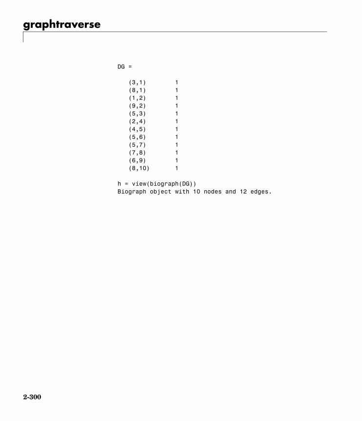
graphtraverse
DG =
(3,1) 1(8,1) 1(1,2) 1(9,2) 1(5,3) 1(2,4) 1(4,5) 1(5,6) 1(5,7) 1(7,8) 1(6,9) 1(8,10) 1
h = view(biograph(DG))Biograph object with 10 nodes and 12 edges.
2-300

graphtraverse
2 Traverse the graph to find the depth-first search (DFS) discoveryorder starting at node 4.
order = graphtraverse(DG,4)
order =
4 5 3 1 2 6 9 7 8 10
2-301

graphtraverse
3 Label the nodes with the DFS discovery order.
for i = 1:10h.Nodes(order(i)).Label =...
sprintf('%s:%d',h.Nodes(order(i)).ID,i);endh.ShowTextInNodes = 'label'dolayout(h)
2-302
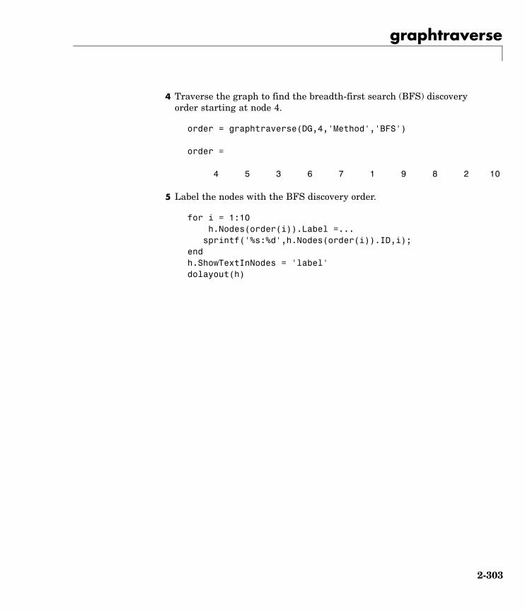
graphtraverse
4 Traverse the graph to find the breadth-first search (BFS) discoveryorder starting at node 4.
order = graphtraverse(DG,4,'Method','BFS')
order =
4 5 3 6 7 1 9 8 2 10
5 Label the nodes with the BFS discovery order.
for i = 1:10h.Nodes(order(i)).Label =...
sprintf('%s:%d',h.Nodes(order(i)).ID,i);endh.ShowTextInNodes = 'label'dolayout(h)
2-303

graphtraverse
6 Find and color nodes that are close to (within two edges of) node 4.
node_idxs = graphtraverse(DG,4,'depth',2)
node_idxs =
4 5 3 6 7
set(h.nodes(node_idxs),'Color',[1 0 0])
2-304
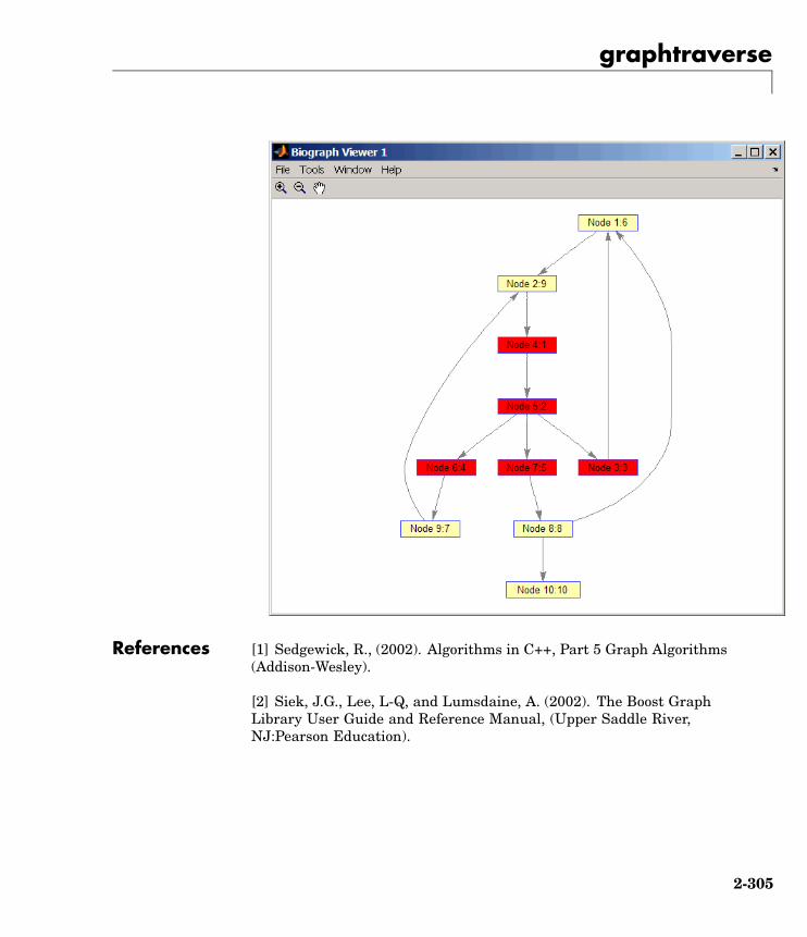
graphtraverse
References [1] Sedgewick, R., (2002). Algorithms in C++, Part 5 Graph Algorithms(Addison-Wesley).
[2] Siek, J.G., Lee, L-Q, and Lumsdaine, A. (2002). The Boost GraphLibrary User Guide and Reference Manual, (Upper Saddle River,NJ:Pearson Education).
2-305

graphtraverse
See Also Bioinformatics Toolbox functions: graphallshortestpaths,graphconncomp, graphisdag, graphisomorphism, graphisspantree,graphmaxflow, graphminspantree, graphpred2path,graphshortestpath, graphtopoorder
Bioinformatics Toolbox method of biograph object: traverse
2-306

hmmprofalign
Purpose Align query sequence to profile using hidden Markov model alignment
Syntax Alignment = hmmprofalign(Model,Seq)[Alignment, Score] = hmmprofalign(Model,Seq)[Score, Alignment, Prointer] = hmmprofalign(Model,Seq)hmmprofalign(..., 'PropertyName', PropertyValue,...)hmmprofalign(..., 'ShowScore', ShowScoreValue)hmmprofalign(..., 'Flanks', FlanksValue)hmmprofalign(..., 'ScoreFlanks', ScoreFlanksValue)hmmprofalign(..., 'ScoreNullTransitions',
ScoreNullTransitionValue)
ArgumentsModel Hidden Markov model created with the
function hmmprofstruct.
Seq Amino acid or nucleotide sequence. Youcan also enter a structure with the fieldSequence.
ShowScoreValue Property to control displaying the scoringspace and the winning path. Enter eithertrue or false (default).
FlanksValue Property to control including the symbolsgenerated by the FLANKING INSERT statesin the output sequence. Enter either true orfalse (default).
ScoreFlanksValue Property to control including the transitionprobabilities for the flanking states in theraw score. Enter either true or false(default).
ScoreNullTransValue Property to control adjusting the rawscore using the null model for transitions(Model.NullX). Enter either true or false(default).
2-307

hmmprofalign
Description Alignment = hmmprofalign(Model,Seq) returns the score for theoptimal alignment of the query amino acid or nucleotide sequence (Seq)to the profile hidden Markov model (Model). Scores are computed usinglog-odd ratios for emission probabilities and log probabilities for statetransitions.
[Alignment, Score] = hmmprofalign(Model,Seq) returns a stringshowing the optimal profile alignment.
Uppercase letters and dashes correspond to MATCH and DELETEstates respectively (the combined count is equal to the number of statesin the model). Lowercase letters are emitted by the INSERT states. Formore information about the HMM profile, see hmmprofstruct.
[Score, Alignment, Prointer] = hmmprofalign(Model,Seq)returns a vector of the same length as the profile model with indicespointing to the respective symbols of the query sequence. Null pointers(NaN) mean that such states did not emit a symbol in the alignedsequence because they represent model jumps from the BEGIN stateof a MATCH state, model jumps from the from a MATCH state to theEND state, or because the alignment passed through DELETE states.
hmmprofalign(..., 'PropertyName', PropertyValue,...) definesoptional properties using property name/value pairs.
hmmprofalign(..., 'ShowScore', ShowScoreValue), whenShowScoreValue is true, displays the scoring space and the winningpath.
hmmprofalign(..., 'Flanks', FlanksValue), when FlanksValueis true, includes the symbols generated by the FLANKING INSERTstates in the output sequence.
hmmprofalign(..., 'ScoreFlanks', ScoreFlanksValue), whenScoreFlanksValue is true, includes the transition probabilities for theflanking states in the raw score.
hmmprofalign(..., 'ScoreNullTransitions',ScoreNullTransitionValue), when ScoreNullTransitionsValueis true, adjusts the raw score using the null model for transitions(Model.NullX).
2-308

hmmprofalign
Note Multiple target alignment is not supported in thisimplementation. All the Model.LoopX probabilities are ignored.
Examples load('hmm_model_examples','model_7tm_2') % load a model example
load('hmm_model_examples','sequences') % load a sequence example
SCCR_RABIT=sequences(2).Sequence;
[a,s]=hmmprofalign(model_7tm_2,SCCR_RABIT,'showscore',true)
See Also Bioinformatics Toolbox functions gethmmprof, hmmprofestimate,hmmprofgenerate, hmmprofgenerate, hmmprofstruct, pfamhmmread,showhmmprof, multialign, profalign
2-309
hmmprofestimate
Purpose Estimate profile Hidden Markov Model (HMM) parameters usingpseudocounts
Syntax hmmprofestimate(Model, MultipleAlignment,'PropertyName', PropertyValue...)
hmmprofestimate(..., 'A', AValue)hmmprofestimate(..., 'Ax', AxValue)hmmprofestimate(..., 'BE', BEValue)hmmprofestimate(..., 'BDx', BDxValue)
ArgumentsModel Hidden Markov model created with the
function hmmprofstruc.
MultipleAlignment Array of sequences. Sequences can also be astructured array with the aligned sequencesin a field Aligned or Sequences, and theoptional names in a field Header or Name.
A Property to set the pseudocount weight A.Default value is 20.
Ax Property to set the pseudocount weight Ax.Default value is 20.
BE Property to set the background symbolemission probabilities. Default values aretaken from Model.NullEmission.
BMx Property to set the background transitionprobabilities from any MATCH state ([M->MM->I M->D]). Default values are taken fromhmmprofstruct.
BDx Property to set the background transitionprobabilities from any DELETE state([D->M D->D]). Default values are taken fromhmmprofstruct.
2-310

hmmprofestimate
Description hmmprofestimate(Model, MultipleAlignment, 'PropertyName',PropertyValue...) returns a structure with the fields containing theupdated estimated parameters of a profile HMM. Symbol emission andstate transition probabilities are estimated using the real counts andweighted pseudocounts obtained with the background probabilities.Default weight is A=20, the default background symbol emission formatch and insert states is taken from Model.NullEmission, and thedefault background transition probabilities are the same as defaulttransition probabilities returned by hmmprofstruct.
Model Construction: Multiple aligned sequences should containuppercase letters and dashes indicating the model MATCH andDELETE states agreeing with Model.ModelLength. If model stateannotation is missing, but MultipleAlignment is space aligned, then a"maximum entropy" criteria is used to select Model.ModelLength states.
Note Insert and flank insert transition probabilities are not estimated,but can be modified afterwards using hmmprofstruct.
hmmprofestimate(..., 'A', AValue) sets the pseudocount weight A= Avalue when estimating the symbol emission probabilities. Defaultvalue is 20.
hmmprofestimate(...,'Ax', AxValue) sets the pseudocount weightAx = Axvalue when estimating the transition probabilities. Defaultvalue is 20.
hmmprofestimate(...,'BE', BEValue) sets the backgroundsymbol emission probabilities. Default values are taken fromModel.NullEmission.
hmmprofestimate(...,'BMx', BMxValue) sets the backgroundtransition probabilities from any MATCH state ([M->M M->I M->D]).Default values are taken from hmmprofstruct.
2-311

hmmprofestimate
hmmprofestimate(..., 'BDx', BDxValue) sets the backgroundtransition probabilities from any DELETE state ([D->M D->D]). Defaultvalues are taken from hmmprofstruct.
See Also Bioinformatics Toolbox functions hmmprofalign, hmmprofstruct,showhmmprof
2-312

hmmprofgenerate
Purpose Generate random sequence drawn from profile Hidden Markov Model(HMM)
Syntax Sequence = hmmprofgenerate(Model)[Sequence, Profptr] = hmmprofgenerate(Model)... = hmmprofgenerate(Model, ...'Align', AlignValue, ...)... = hmmprofgenerate(Model, ...'Flanks', FlanksValue, ...)... = hmmprofgenerate(Model, ...'Signature', SignatureValue,
...)
ArgumentsModel Hidden Markov model created with the
hmmprofstruct function.
AlignValue Property to control using uppercase lettersfor matches and lowercase letters for insertedletters. Enter either true or false. Defaultis false.
FlanksValue Property to control including the symbolsgenerated by the FLANKING INSERT statesin the output sequence. Enter either true orfalse. Default is false.
SignatureValue Property to control returning the most likelypath and symbols. Enter either true or false.Default is false.
Description Sequence = hmmprofgenerate(Model) returns the string Sequenceshowing a sequence of amino acids or nucleotides drawn from theprofile Model. The length, alphabet, and probabilities of the Model arestored in a structure. For move information about this structure, seehmmprofstruct.
[Sequence, Profptr] = hmmprofgenerate(Model) returns a vector of thesame length as the profile model pointing to the respective states in theoutput sequence. Null pointers (0) mean that such states do not exist inthe output sequence, either because they are never touched (i.e., jumps
2-313

hmmprofgenerate
from the BEGIN state to MATCH states or from MATCH states to theEND state), or because DELETE states are not in the output sequence(not aligned output; see below).
... = hmmprofgenerate(Model, ...'PropertyName',PropertyValue, ...) calls hmmprofgenerate with optional propertiesthat use property name/property value pairs. You can specify one ormore properties in any order. Each PropertyName must be enclosed insingle quotes and is case insensitive. These property name/propertyvalue pairs are as follows:
... = hmmprofgenerate(Model, ...'Align', AlignValue, ...) ifAlign is true, the output sequence is aligned to the model as follows:uppercase letters and dashes correspond to MATCH and DELETEstates respectively (the combined count is equal to the number ofstates in the model). Lowercase letters are emitted by the INSERT orFLANKING INSERT states. If AlignValue is false, the output is asequence of uppercase symbols. The default value is true.
... = hmmprofgenerate(Model, ...'Flanks', FlanksValue, ...) ifFlanks is true, the output sequence includes the symbols generated bythe FLANKING INSERT states. The default value is false.
... = hmmprofgenerate(Model, ...'Signature',SignatureValue, ...) if SignatureValue is true, returns the mostlikely path and symbols. The default value is false.
Examples load('hmm_model_examples','model_7tm_2') % load a model examplerand_sequence = hmmprofgenerate(model_7tm_2)
See Also Bioinformatics Toolbox functions: hmmprofalign, hmmprofstruct,showhmmprof
2-314
hmmprofmerge
Purpose Concatenate prealigned strings of several sequences to profile HiddenMarkow Model (HMM)
Syntax hmmprofmerge(Sequences)hmmprofmerge(Sequences, Names)hmmprofmerge(Sequences, Names, Scores)
ArgumentsSequences Array of sequences. Sequences can also be a
structured array with the aligned sequences in a fieldAligned or Sequences, and the optional names in afield Header or Name.
Names Names for the sequences. Enter a vector of names.
Scores Pairwise alignment scores from the functionhmmprofalign. Enter a vector of values with the samelength as the number of sequences in Sequences.
Description hmmprofmerge(Sequences) displays a set of prealigned sequences to aHMM model profile. The output is aligned corresponding to the HMMstates.
• Match states — Uppercase letters
• Insert states — Lowercase letters or asterisks (*)
• Delete states — Dashes
Periods (.) are added at positions corresponding to inserts in othersequences. The input sequences must have the same number of profilestates, that is, the joint count of capital letters and dashes must bethe same.
hmmprofmerge(Sequences, Names) labels the sequences with Names.
hmmprofmerge(Sequences, Names, Scores) sorts the displayedsequences using Scores.
2-315
hmmprofmerge
Examples load('hmm_model_examples','model_7tm_2') %load modelload('hmm_model_examples','sequences') %load sequences
for ind =1:length(sequences)[scores(ind),sequences(ind).Aligned] =...
hmmprofalign(model_7tm_2,sequences(ind).Sequence);end
hmmprofmerge(sequences, scores)
See Also Bioinformatics Toolbox functions: hmmprofalign, hmmprofstruct
2-316
hmmprofstruct
Purpose Create profile Hidden Markov Model (HMM) structure
Syntax Model = hmmprofstruct(Length)Model = hmmprofstruct(Length, 'Field1', FieldValues1,...)hmmprofstruct(Model, 'Field1', Field1Values1,...)
Arguments Length Number of match states in the model.
Model Hidden Markov model created with the functionhmmprofstruct.
Field1 Field name in the structure Model. Enter a namefrom the table below.
Description Model = hmmprofstruct(Length) returns a structure with the fieldscontaining the required parameters of a profile HMM. Length specifiesthe number of match states in the model. All other mandatory modelparameters are initialized to the default values.
Model = hmmprofstruct(Length, 'Field1', FieldValues1, ...)creates a profile HMM using the specified fields and parameters. Allother mandatory model parameters are initialized to default values.
hmmprofstruct(Model, 'Field1', Field1Values1, ...) returnsthe updated profile HMM with the specified fields and parameters.All other mandatory model parameters are taken from the referenceMODEL.
HMM Profile Structure Format
Model parameters fields (mandatory). All probability values are in the[0 1] range.
Field Name Description
ModelLength Length of the profile (number of MATCH states)
Alphabet 'AA' or 'NT'. Default is 'AA'.
2-317

hmmprofstruct
Field Name Description
MatchEmission Symbol emission probabilities in the MATCHstates.
Size is [ModelLength x AlphaLength]. Defaults touniform distributions. May accept a structure withresidue counts (see aacount or basecount).
InsertEmission Symbol emission probabilities in the INSERTstate.
Size is [ModelLength x AlphaLength]. Defaults touniform distributions. May accept a structure withresidue counts (see aacount or basecount).
NullEmission Symbol emission probabilities in the MATCH andINSERT states for the NULL model. NULL model,size is [1 x AlphaLength]. Defaults to a uniformdistribution. May accept a structure with residuecounts (see aacount or basecount). The NULLmodel is used to compute the log-odds ratio atevery state and avoid overflow when propagatingthe probabilities through the model.
BeginX BEGIN state transition probabilities.
Format is
[B->D1 B->M1 B->M2 B->M3 .... B->Mend]
Notes:
sum(S.BeginX) = 1
For fragment profiles
sum(S.BeginX(3:end)) = 0
Default is [0.01 0.99 0 0 ... 0].
2-318

hmmprofstruct
Field Name Description
MatchX MATCH state transition probabilities
Format is
[M1->M2 M2->M3 ... M[end-1]->Mend;M1->I1 M2->I2 ... M[end-1]->I[end-1];M1->D2 M2->D3 ... M[end-1]->Dend;M1->E M2->E ... M[end-1]->E ]
Notes:
sum(S.MatchX) = [ 1 1 ... 1 ]
For fragment profiles
sum(S.MatchX(4,:)) = 0
Default is repmat([0.998 0.001 0.0010],profLength-1,1).
InsertX INSERT state transition probabilities
Format is
[I1->M2 I2->M3 ... I[end-1]->Mend;[I1->I1 I2->I2 ... I[end-1]->I[end-1] ]
Note:
sum(S.InsertX) = [ 1 1 ... 1 ]
Default is repmat([0.5 0.5],profLength-1,1).
2-319

hmmprofstruct
Field Name Description
DeleteX DELETE state transition probabilities. The formatis
[D1->M2 D2->M3 ... D[end-1]->Mend ;[D1->D2 D2->D3 ... D[end-1]->Dend ]
Note sum(S.DeleteX) = [ 1 1 ... 1 ]
Default is repmat([0.5 0.5],profLength-1,1).
FlankingInsertX Flanking insert states (N and C) used for LOCALprofile alignment. The format is
[N->B C->T ;[N->N C->C ]
Note sum(S.FlankingInsertsX) = [1 1]
To force global alignment use
S.FlankingInsertsX = [1 1; 0 0]
Default is [0.01 0.01; 0.99 0.99].
2-320
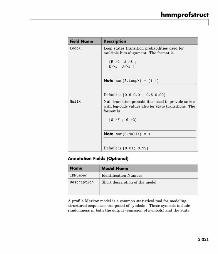
hmmprofstruct
Field Name Description
LoopX Loop states transition probabilities used formultiple hits alignment. The format is
[E->C J->B ;E->J J->J ]
Note sum(S.LoopX) = [1 1]
Default is [0.5 0.01; 0.5 0.99]
NullX Null transition probabilities used to provide scoreswith log-odds values also for state transitions. Theformat is
[G->F ; G->G]
Note sum(S.NullX) = 1
Default is [0.01; 0.99]
Annotation Fields (Optional)
Name Model Name
IDNumber Identification Number
Description Short description of the model
A profile Markov model is a common statistical tool for modelingstructured sequences composed of symbols . These symbols includerandomness in both the output (emission of symbols) and the state
2-321

hmmprofstruct
transitions of the process. Markov models are generally representedby state diagrams.
The figure shown below is a state diagram for a HMM profile of length 4.Insert, match, and delete states are in the regular part (middle section).
• Match state means that the target sequence is aligned to the profileat the specific location.
• Delete state represents a gap or symbol absence in the targetsequence (also know as a silent state because it does not emit anysymbol).
• Insert state represents the excess of one or more symbols in thetarget sequence that are not included in the profile.
Flanking states (S, N, B, E, C, T) are used for proper modeling of theends of the sequence, either for global, local or fragment alignment ofthe profile. S, N, E, and T are silent while N and C are used to insertsymbols at the flanks.
Examples hmmprofstruct(100,'Alphabet','AA')
See Also Bioinformatics Toolbox functions: aacount, basecount, gethmmprof,hmmprofalign, hmmprofestimate, hmmprofgenerate, hmmprofmerge,pfamhmmread, showhmmprof
2-322

imageneread
Purpose Read microarray data from ImaGene Results file
Syntax imagenedata = imageneread('File')imagenedata = imageneread(..., 'CleanColNames',CleanColNamesValue, ...)
ArgumentsFile ImaGene Results formatted file. Enter a file
name or a path and file name.
CleanColNameValue Property to control creating column names thatMATLAB can use as variable names.
Description imagenedata = imageneread('File') reads ImaGene results datafrom File and creates a MATLAB structure imagedata containing thefollowing fields:
Field
HeaderAA
Data
Blocks
Rows
Columns
Fields
IDs
ColumnNames
2-323
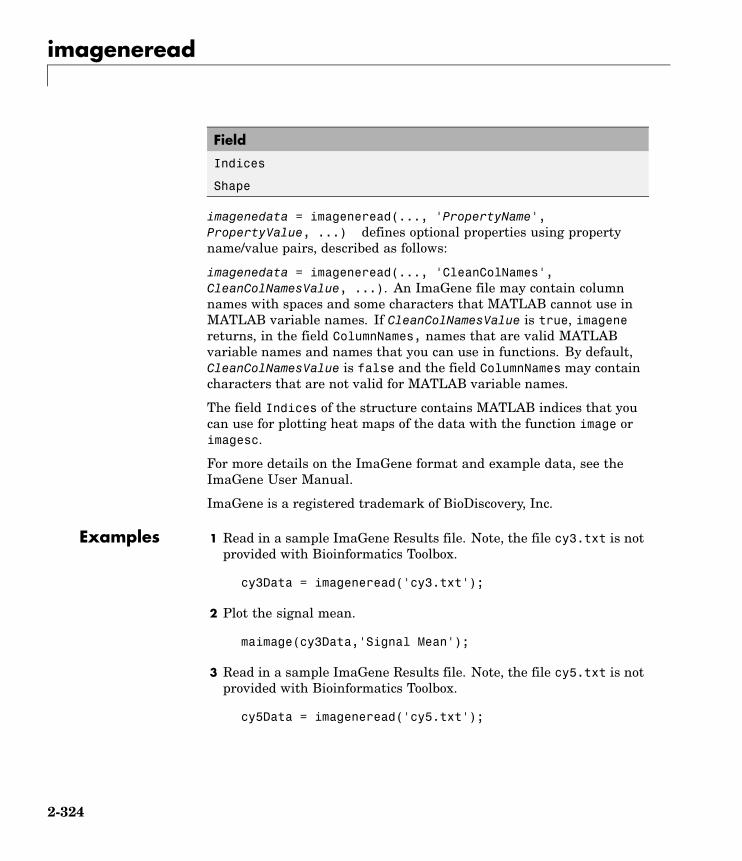
imageneread
Field
Indices
Shape
imagenedata = imageneread(..., 'PropertyName',PropertyValue, ...) defines optional properties using propertyname/value pairs, described as follows:
imagenedata = imageneread(..., 'CleanColNames',CleanColNamesValue, ...). An ImaGene file may contain columnnames with spaces and some characters that MATLAB cannot use inMATLAB variable names. If CleanColNamesValue is true, imagenereturns, in the field ColumnNames, names that are valid MATLABvariable names and names that you can use in functions. By default,CleanColNamesValue is false and the field ColumnNames may containcharacters that are not valid for MATLAB variable names.
The field Indices of the structure contains MATLAB indices that youcan use for plotting heat maps of the data with the function image orimagesc.
For more details on the ImaGene format and example data, see theImaGene User Manual.
ImaGene is a registered trademark of BioDiscovery, Inc.
Examples 1 Read in a sample ImaGene Results file. Note, the file cy3.txt is notprovided with Bioinformatics Toolbox.
cy3Data = imageneread('cy3.txt');
2 Plot the signal mean.
maimage(cy3Data,'Signal Mean');
3 Read in a sample ImaGene Results file. Note, the file cy5.txt is notprovided with Bioinformatics Toolbox.
cy5Data = imageneread('cy5.txt');
2-324

imageneread
4 Create a loglog plot of the signal median from two ImaGene Resultsfiles.
sigMedianCol = find(strcmp('Signal Median',cy3Data.ColumnNames));
cy3Median = cy3Data.Data(:,sigMedianCol);
cy5Median = cy5Data.Data(:,sigMedianCol);
maloglog(cy3Median,cy5Median,'title','Signal Median');
See Also Bioinformatics Toolbox functions: gprread, maboxplot, maimage,sptread
2-325

int2aa
Purpose Convert amino acid sequence from integer to letter representation
Syntax SeqChar = int2aa(SeqInt)SeqChar = int2aa(SeqInt, 'Case', CaseValue)
Arguments SeqInt Row vector of integers specifying an amino acidsequence. See the table Mapping Amino Acid Integersto Letters on page 2-326 for valid integers. Integers arearbitrarily assigned to IUB/IUPAC letters.
CaseValue String that specifies the case of the returned characterstring. Choices are 'upper' (default) or 'lower'.
ReturnValues
SeqChar Character string of single-letter codes specifying anamino acid sequence.
Mapping Amino Acid Integers to Letters
Amino Acid Integer Code
Alanine 1 A
Arginine 2 R
Asparagine 3 N
Aspartic acid (Aspartate) 4 D
Cysteine 5 C
Glutamine 6 Q
Glutamic acid (Glutamate) 7 E
Glycine 8 G
2-326

int2aa
Amino Acid Integer Code
Histidine 9 H
Isoleucine 10 I
Leucine 11 L
Lysine 12 K
Methionine 13 M
Phenylalanine 14 F
Proline 15 P
Serine 16 S
Threonine 17 T
Tryptophan 18 W
Tyrosine 19 Y
Valine 20 V
Aspartic acid or Asparagine 21 B
Glutamic acid or glutamine 22 Z
Any amino acid 23 X
Translation stop 24 *
Gap of indeterminate length 25 -
Unknown or any integer not intable
0 ?
Description SeqChar = int2aa(SeqInt) converts a 1-by-N array of integersspecifying an amino acid sequence to a character string of single-lettercodes specifying the same amino acid sequence. See the table MappingAmino Acid Integers to Letters on page 2-326 for valid integers.
2-327

int2aa
SeqChar = int2aa(SeqInt, 'Case', CaseValue) specifies the caseof the returned character string representing an amino acid sequence.Choices are 'upper' (default) or 'lower'.
Examples Convert an amino acid sequence from integer to letter representation.
s = int2aa([13 1 17 11 1 21])
s =
MATLAB
See Also Bioinformatics Toolbox functions: aa2int, aminolookup, int2nt,nt2int
2-328

int2nt
Purpose Convert nucleotide sequence from integer to letter representation
Syntax int2nt(SeqNT)int2nt(..., 'PropertyName', PropertyValue,...)int2nt(..., 'Alphabet', AlphabetValue)int2nt(..., 'Unknown', UnknownValue)int2nt(..., 'Case', CaseValue)
ArgumentsSeqNT Nucleotide sequence represented by integers.
Enter a vector of integers from the tableMapping Nucleotide Integers to Letters below.The array does not have to be of type integer,but it does have to contain only integernumbers. Integers are arbitrarily assigned toIUB/IUPAC letters.
AlphabetValue Property to select the nucleotide alphabet.Enter either 'DNA' or 'RNA'.
UnknownValue Property to select the integer value for theunknown character. Enter a character tomap integers 16 or greater to an unknowncharacter. The character must not be oneof the nucleotide characters A, T, C, G or theambiguous nucleotide characters N, R, Y, K, M, S,W, B, D, H, or V. The default character is *.
CaseValue Property to select the letter case for thenucleotide sequence. Enter either 'upper'(default) or 'lower' .
2-329
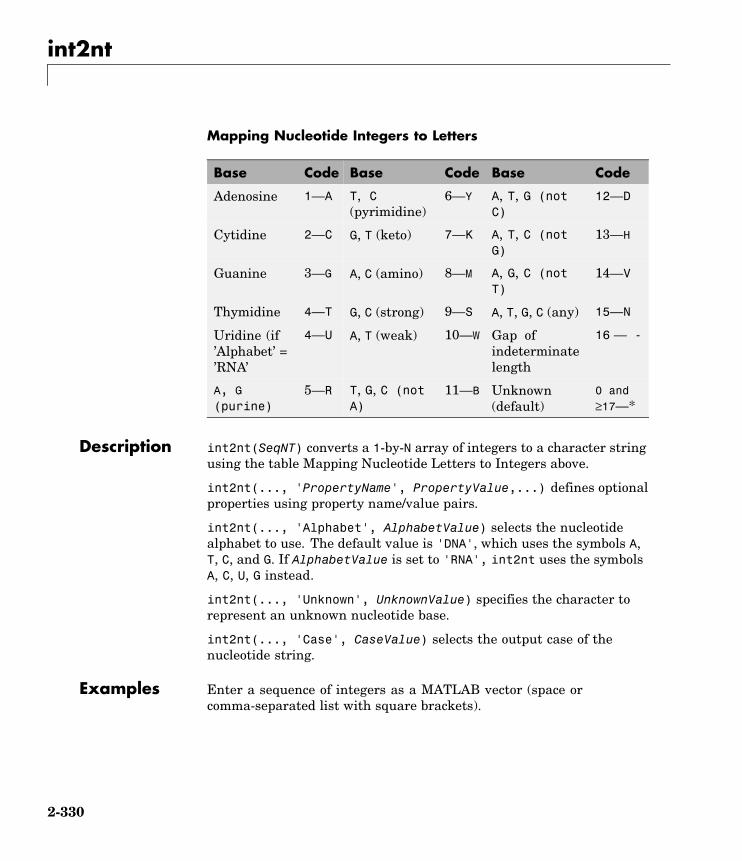
int2nt
Mapping Nucleotide Integers to Letters
Base Code Base Code Base Code
Adenosine 1—A T, C(pyrimidine)
6—Y A, T, G (notC)
12—D
Cytidine 2—C G, T (keto) 7—K A, T, C (notG)
13—H
Guanine 3—G A, C (amino) 8—M A, G, C (notT)
14—V
Thymidine 4—T G, C (strong) 9—S A, T, G, C (any) 15—N
Uridine (if’Alphabet’ =’RNA’
4—U A, T (weak) 10—W Gap ofindeterminatelength
16 — -
A, G(purine)
5—R T, G, C (notA)
11—B Unknown(default)
0 and≥17—*
Description int2nt(SeqNT) converts a 1-by-N array of integers to a character stringusing the table Mapping Nucleotide Letters to Integers above.
int2nt(..., 'PropertyName', PropertyValue,...) defines optionalproperties using property name/value pairs.
int2nt(..., 'Alphabet', AlphabetValue) selects the nucleotidealphabet to use. The default value is 'DNA', which uses the symbols A,T, C, and G. If AlphabetValue is set to 'RNA', int2nt uses the symbolsA, C, U, G instead.
int2nt(..., 'Unknown', UnknownValue) specifies the character torepresent an unknown nucleotide base.
int2nt(..., 'Case', CaseValue) selects the output case of thenucleotide string.
Examples Enter a sequence of integers as a MATLAB vector (space orcomma-separated list with square brackets).
2-330

int2nt
s = int2nt([1 2 4 3 2 4 1 3 2])
s =ACTGCTAGC
Define a symbol for unknown numbers 16 and greater.
si = [1 2 4 20 2 4 40 3 2];s = int2nt(si, 'unknown', '#')
s =ACT#CT#GC
See Also Bioinformatics Toolbox function aa2int, int2aa, nt2int
2-331
isoelectric
Purpose Estimate isoelectric point for amino acid sequence
Syntax pI = isoelectric(SeqAA)[pI Charge] = isoelectric(SeqAA)isoelectric(..., 'PropertyName', PropertyValue,...)isoelectric(..., 'PKVals', PKValsValue)isoelectric(..., 'Charge', ChargeValue)isoelectric(..., 'Chart', ChartValue)
ArgumentsSeqAA Amino acid sequence. Enter a character string or a
vector of integers from the table. Examples: 'ARN'or [1 2 3].
PKValsValue Property to provide alternative pK values.
ChargeValue Property to select a specific pH for estimating charge.Enter a number between 0 and 14. The default valueis 7.2.
ChartValue Property to control plotting a graph of charge versuspH. Enter true or false.
Description pI = isoelectric(SeqAA) returns the estimated isoelectric point (pI)for an amino acid sequence. The isoelectric point is the pH at which theprotein has a net charge of zero
[pI Charge] = isoelectric(SeqAA) returns the estimated isoelectricpoint (pI) for an amino acid sequence and the estimated charge for agiven pH (default is typical intracellular pH 7.2).
The estimates are skewed by the underlying assumptions that all aminoacids are fully exposed to the solvent, that neighboring peptides have noinfluence on the pK of any given amino acid, and that the constitutiveamino acids, as well as the N- and C-termini, are unmodified. Cysteine
2-332

isoelectric
residues participating in disulfide bridges also affect the true pI and arenot considered here. By default, isoelectric uses the EMBOSS aminoacid pK table, or you can substitute other values using the propertyPKVals.
• If the sequence contains ambiguous amino acid characters (b z * –),isoelectric ignores the characters and displays a warning message.
Warning: Symbols other than the standard 20 amino acidsappear in the sequence.
• If the sequence contains undefined amino acid characters (i j o) ,isoelectric ignores the characters and displays a warning message.
Warning: Sequence contains unknown characters. These willbe ignored.
isoelectric(..., 'PropertyName', PropertyValue,...) definesoptional properties using property name/value pairs.
isoelectric(..., 'PKVals', PKValsValue) uses the alternativepK table stored in the text file PKValValues. For an example of a pKtext file, see the file Emboss.pK.
N_term 8.6K 10.8R 12.5H 6.5D 3.9E 4.1C 8.5Y 10.1C_term 3.6
isoelectric(..., 'Charge', ChargeValue) returns the estimatedcharge of a sequence for a given pH (ChargeValue).
2-333
isoelectric
isoelectric(..., 'Chart', ChartValue) when ChartValue is true,returns a graph plotting the charge of the protein versus the pH of thesolvent.
Example % Get a sequence from PDB.pdbSeq = getpdb('1CIV', 'SequenceOnly', true)% Estimate its isoelectric point.isoelectric(pdbSeq)
% Plot the charge against the pH for a short polypeptide sequence.isoelectric('PQGGGGWGQPHGGGWGQPHGGGGWGQGGSHSQG', 'CHART', true)
% Get the Rh blood group D antigen from NCBI and calculate% its charge at pH 7.3 (typical blood pH).gpSeq = getgenpept('AAB39602')[pI Charge] = isoelectric(gpSeq, 'Charge', 7.38)
See Also Bioinformatics functions aacount, molweight
2-334

jcampread
Purpose Read JCAMP-DX formatted files
Syntax JCAMPData = jcampread(File)
ArgumentsFile JCAMP-DX formatted file (ASCII text file). Enter a
file name, a path and file name, or a URL pointing to afile. File can also be a MATLAB character array thatcontains the text of a JCAMP-DX formatted file.
Description JCAMP-DX is a file format for infrared, NMR, and mass spectrometrydata from the Joint Committee on Atomic and Molecular Physical Data(JCAMP). jcampread supports reading data from files saved withVersions 4.24 and 5 of the JCAMP-DX format. For more details, see
http://www.jcamp.org/index.html
JCAMPData = jcampread(File)reads data from a JCAMP-DXformatted file (File) and creates a MATLAB structure (JCAMPData)containing the following fields:
Field
Title
DataType
Origin
Owner
Blocks
Notes
The Blocks field of the structure is an array of structures correspondingto each set of data in the file. These structures have the following fields:
2-335
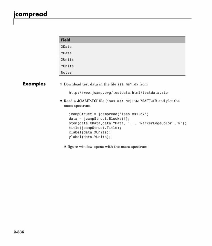
jcampread
Field
XData
YData
XUnits
YUnits
Notes
Examples 1 Download test data in the file isa_ms1.dx from
http://www.jcamp.org/testdata.html/testdata.zip
2 Read a JCAMP-DX file (isas_ms1.dx) into MATLAB and plot themass spectrum.
jcampStruct = jcampread('isas_ms1.dx')data = jcampStruct.Blocks(1);stem(data.XData,data.YData, '.', 'MarkerEdgeColor','w');title(jcampStruct.Title);xlabel(data.XUnits);ylabel(data.YUnits);
A figure window opens with the mass spectrum.
2-336
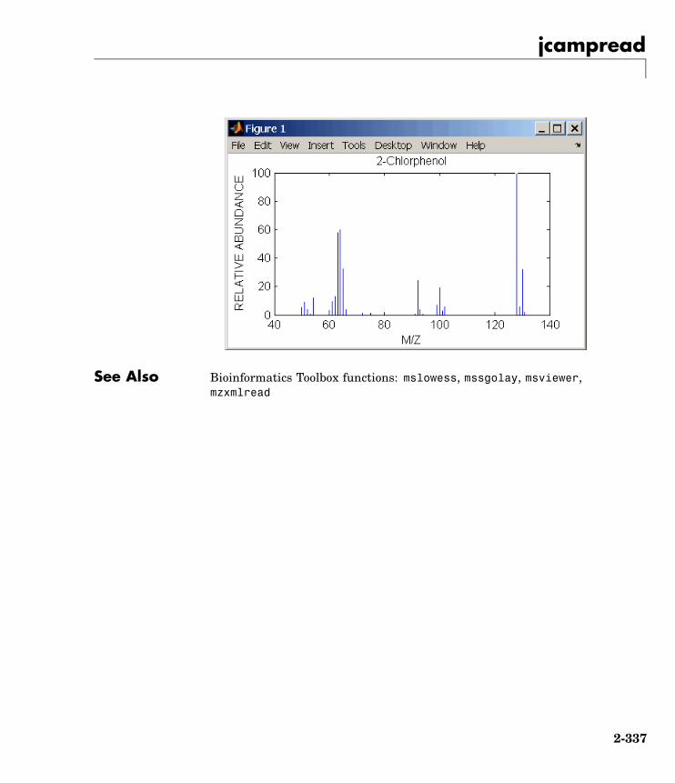
jcampread
See Also Bioinformatics Toolbox functions: mslowess, mssgolay, msviewer,mzxmlread
2-337
joinseq
Purpose Join two sequences to produce shortest supersequence
Syntax SeqNT3 = joinseq(SeqNT1, SeqNT2)
ArgumentsSeqNT1, SeqNT2 Nucleotide sequences.
Description SeqNT3 = joinseq(SeqNT1, SeqNT2) creates a new sequence thatis the shortest supersequence of SeqNT1 and SeqNT2. If there is nooverlap between the sequences, then SeqNT2 is concatenated to the endof SeqNT1. If the length of the overlap is the same at both ends of thesequence, then the overlap at the end of SeqNT1 and the start of SeqNT2is used to join the sequences.
If SeqNT1 is a subsequence of SeqNT2, then SeqNT2 is returned as theshortest supersequence and vice versa.
Examples seq1 = 'ACGTAAA';seq2 = 'AAATGCA';joined = joinseq(seq1,seq2)
joined =ACGTAAATGCA
See Also MATLAB functions cat, strcat, strfind
2-338

knnclassify
Purpose Classify data using nearest neighbor method
Syntax Class = knnclassify(Sample, Training, Group)Class = knnclassify(Sample, Training, Group, k)Class = knnclassify(Sample, Training, Group, k, distance)Class = knnclassify(Sample, Training, Group, k, distance,
rule)
ArgumentsSample Matrix whose rows will be classified into groups. Sample
must have the same number of columns as Training.
Training Matrix used to group the rows in the matrix Sample.Training must have the same number of columns asSample. Each row of Training belongs to the groupwhose value is the corresponding entry of Group.
Group Vector whose distinct values define the grouping of therows in Training.
k The number of nearest neighbors used in theclassification. Default is 1.
2-339
knnclassify
distance String to specify the distance metric. Choices are:• 'euclidean' — Euclidean distance (default)
• 'cityblock' — Sum of absolute differences
• 'cosine' — One minus the cosine of the includedangle between points (treated as vectors)
• 'correlation' — One minus the sample correlationbetween points (treated as sequences of values)
• 'hamming' — Percentage of bits that differ (onlysuitable for binary data)
rule String to specify the rule used to decide how to classifythe sample. Choices are:• 'nearest' — Majority rule with nearest point
tie-break (default)
• 'random' — Majority rule with random pointtie-break
• 'consensus' — Consensus rule
Description Class = knnclassify(Sample, Training, Group) classifies the rowsof the data matrix Sample into groups, based on the grouping of the rowsof Training. Sample and Training must be matrices with the samenumber of columns. Group is a vector whose distinct values define thegrouping of the rows in Training. Each row of Training belongs to thegroup whose value is the corresponding entry of Group. knnclassifyassigns each row of Sample to the group for the closest row of Training.Group can be a numeric vector, a string array, or a cell array of strings.Training and Group must have the same number of rows. knnclassifytreats NaNs or empty strings in Group as missing values, and ignoresthe corresponding rows of Training. Class indicates which group eachrow of Sample has been assigned to, and is of the same type as Group.
Class = knnclassify(Sample, Training, Group, k) enables you tospecify k, the number of nearest neighbors used in the classification.Default is 1.
2-340
knnclassify
Class = knnclassify(Sample, Training, Group, k, distance)enables you to specify the distance metric. Choices for distance are:
'euclidean' Euclidean distance (default)
'cityblock' Sum of absolute differences
'cosine' One minus the cosine of the included angle betweenpoints (treated as vectors)
'correlation' One minus the sample correlation between points(treated as sequences of values)
'hamming' Percentage of bits that differ (only suitable for binarydata)
Class = knnclassify(Sample, Training, Group, k,distance, rule) enables you to specify the rule used to decide how toclassify the sample. Choices for rule are:
'nearest' Majority rule with nearest point tie-break (default)
'random' Majority rule with random point tie-break
'consensus' Consensus rule
The default behavior is to use majority rule. That is, a sample point isassigned to the class the majority of the k nearest neighbors are from.Use 'consensus' to require a consensus, as opposed to majority rule.When using the 'consensus' option, points where not all of the knearest neighbors are from the same class are not assigned to one of theclasses. Instead the output Class for these points is NaN for numericalgroups or '' for string named groups. When classifying to more thantwo groups or when using an even value for k, it might be necessary tobreak a tie in the number of nearest neighbors. Options are 'random',which selects a random tiebreaker, and 'nearest', which uses thenearest neighbor among the tied groups to break the tie. The defaultbehavior is majority rule, with nearest tie-break.
2-341

knnclassify
Examples Classifying Rows
The following example classifies the rows of the matrix sample:
sample = [.9 .8;.1 .3;.2 .6]
sample =0.9000 0.80000.1000 0.30000.2000 0.6000
training=[0 0;.5 .5;1 1]
training =0 0
0.5000 0.50001.0000 1.0000
group = [1;2;3]
group =123
class = knnclassify(sample, training, group)
class =312
Row 1 of sample is closest to row 3 of Training, so class(1) = 3. Row2 of sample is closest to row 1 of Training, so class(2) = 1. Row 3 ofsample is closest to row 2 of Training, so class(3) = 2.
2-342
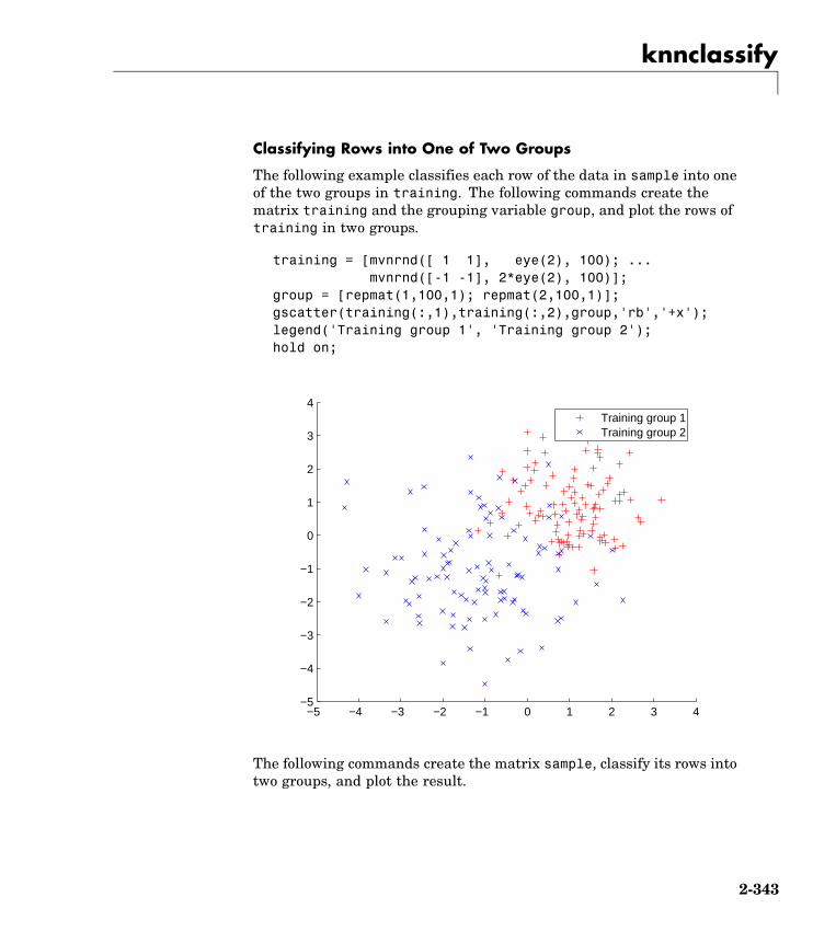
knnclassify
Classifying Rows into One of Two Groups
The following example classifies each row of the data in sample into oneof the two groups in training. The following commands create thematrix training and the grouping variable group, and plot the rows oftraining in two groups.
training = [mvnrnd([ 1 1], eye(2), 100); ...mvnrnd([-1 -1], 2*eye(2), 100)];
group = [repmat(1,100,1); repmat(2,100,1)];gscatter(training(:,1),training(:,2),group,'rb','+x');legend('Training group 1', 'Training group 2');hold on;
−5 −4 −3 −2 −1 0 1 2 3 4−5
−4
−3
−2
−1
0
1
2
3
4Training group 1Training group 2
The following commands create the matrix sample, classify its rows intotwo groups, and plot the result.
2-343

knnclassify
sample = unifrnd(-5, 5, 100, 2);% Classify the sample using the nearest neighbor classificationc = knnclassify(sample, training, group);gscatter(sample(:,1),sample(:,2),c,'mc'); hold on;legend('Training group 1','Training group 2', ...
'Data in group 1','Data in group 2');hold off;
−5 0 5−5
−4
−3
−2
−1
0
1
2
3
4
5Training group 1Training group 2Data in group 1Data in group 2
Classifying Rows Using the Three Nearest Neighbors
The following example uses the same data as in Example 2, but classifiesthe rows of sample using three nearest neighbors instead of one.
gscatter(training(:,1),training(:,2),group,'rb',+x');
hold on;
c3 = knnclassify(sample, training, group, 3);
2-344
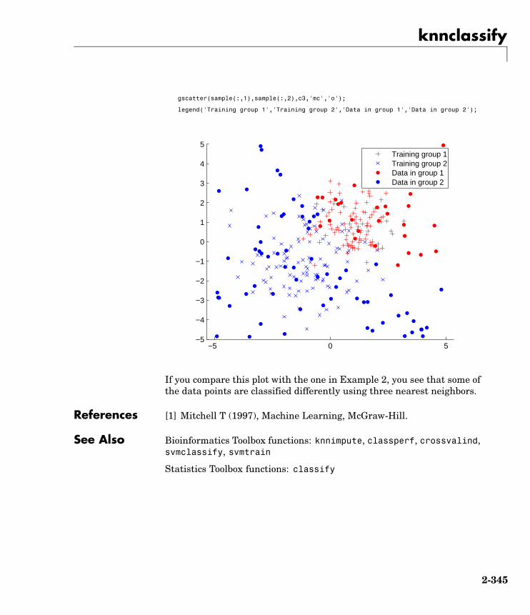
knnclassify
gscatter(sample(:,1),sample(:,2),c3,'mc','o');
legend('Training group 1','Training group 2','Data in group 1','Data in group 2');
−5 0 5−5
−4
−3
−2
−1
0
1
2
3
4
5Training group 1Training group 2Data in group 1Data in group 2
If you compare this plot with the one in Example 2, you see that some ofthe data points are classified differently using three nearest neighbors.
References [1] Mitchell T (1997), Machine Learning, McGraw-Hill.
See Also Bioinformatics Toolbox functions: knnimpute, classperf, crossvalind,svmclassify, svmtrain
Statistics Toolbox functions: classify
2-345

knnimpute
Purpose Impute missing data using nearest-neighbor method
Syntax knnimpute(Data)knnimpute(Data, k)knnimpute(..., 'PropertyName', PropertyValue,...)knnimpute(..., 'Distance', DistanceValue)knnimpute(..., 'DistArgs', DistArgsValue)knnimpute(..., 'Weights', WeightsValues)knnimpute(..., 'Median', MedianValue)
ArgumentsData
k
Description knnimpute(Data)replaces NaNs in Data with the corresponding valuefrom the nearest-neighbor column. The nearest-neighbor column isthe closest column in Euclidean distance. If the corresponding valuefrom the nearest-neighbor column is also NaN, the next nearest columnis used.
knnimpute(Data, k)replaces NaNs in Data with a weighted mean of thek nearest-neighbor columns. The weights are inversely proportional tothe distances from the neighboring columns.
knnimpute(..., 'PropertyName', PropertyValue,...) definesoptional properties using property name/value pairs.
knnimpute(..., 'Distance', DistanceValue) computesnearest-neighbor columns using the distance metric distfun. Thechoices for DistanceValue are
'euclidean' Euclidean distance (default).
'seuclidean' Standardized Euclidean distance — each coordinatein the sum of squares is inversely weighted by thesample variance of that coordinate.
2-346

knnimpute
'cityblock' City block distance
'mahalanobis'Mahalanobis distance
'minkowski' Minkowski distance with exponent 2
'cosine' One minus the cosine of the included angle
'correlation'One minus the sample correlation betweenobservations, treated as sequences of values
'hamming' Hamming distance — the percentage of coordinatesthat differ
'jaccard' One minus the Jaccard coefficient — the percentageof nonzero coordinates that differ
'chebychev' Chebychev distance (maximum coordinate difference)
functionhandle
A handle to a distance function, specified using @, forexample @distfun
See pdist for more details.
knnimpute(..., 'DistArgs', DistArgsValue) passes arguments(DistArgsValue) to the function distfun. DistArgsValue can be asingle value or a cell array of values.
knnimpute(..., 'Weights', WeightsValues) enables you to specifythe weights used in the weighted mean calculation. w should be a vectorof length k.
knnimpute(..., 'Median', MedianValue) when MedianValue istrue, uses the median of the k nearest neighbors instead of theweighted mean.
Example 1 A = [1 2 5;4 5 7;NaN -1 8;7 6 0]
A =
1 2 54 5 7
2-347

knnimpute
NaN -1 87 6 0
Note that A(3,1) = NaN. Because column 2 is the closest column tocolumn 1 in Euclidean distance, knnimpute imputes the (3,1) entry ofcolumn 1 to be the corresponding entry of column 2, which is -1.
knnimpute(A)
ans =
1 2 54 5 7
-1 -1 87 6 0
Example 2 The following example loads the data set yeastdata and imputesmissing values in the array yeastvalues.
load yeastdata% Remove data for empty spotsemptySpots = strcmp('EMPTY',genes);yeastvalues(emptySpots,:) = [];genes(emptySpots) = [];% Impute missing valuesimputedValues = knnimpute(yeastvalues);
References [1] Speed T (2003), Statistical Analysis of Gene Expression MicroarrayData, Chapman & Hall/CRC.
[2] Hastie T, Tibshirani R, Sherlock G. Eisen M, Brown P, Botstein D(1999), “Imputing missing data for gene expression arrays”, TechnicalReport, Division of Biostatistics, Stanford University.
[3] Troyanskaya O, Cantor M, Sherlock G, Brown P, Hastie T, TibshiraniR, Botstein D, Altman R (2001), “Missing value estimation methods forDNA microarrays”, Bioinformatics, 17( 6)520-525.
2-348

knnimpute
See Also Bioinformatics Toolbox function knnclassify
MATLAB function isnan
Statistics Toolbox functions nanmean, nanmedian, pdist
2-349

maboxplot
Purpose Box plot for microarray data
Syntax maboxplot(MAData)maboxplot(MAData, ColumnName)maboxplot(MAStruct, FieldName)H = maboxplot(...)[H, HLines] = maboxplot(...)maboxplot(..., 'PropertyName', PropertyValue, ...)maboxplot(..., 'Title', TitleValue, ...)maboxplot(..., 'Notch', NotchValue, ...)maboxplot(..., 'Symbol', SymbolValue, ...)maboxplot(..., 'Orientation', OrientationValue, ...)maboxplot(..., 'WhiskerLength', WhiskerLengthValue, ...)
ArgumentsMAData A numeric array or a structure containing a
field called Data. The values in the columnsof MAData will be used to create box plots.
ColumnName An array of column names corresponding tothe data in MAData.
MAStruct A microarray data structure.
FieldName A field within the microarray data structure,MAStruct. The values in the field FieldNamewill be used to create box plots.
TitleValue A string to use as the title for the plot. Thedefault title is FieldName.
NotchValue Property to control the type of boxes drawn.Enter either true for notched boxes, orfalse, for square boxes. Default is false.
2-350

maboxplot
OrientationValue Property to specify the orientation of the boxplot. Enter 'Vertical' or 'Horizontal'.Default is 'Horizontal'.
WhiskerLengthValue Property to specify the maximum lengthof the whiskers as a function of theinterquartile range (IQR). The whiskerextends to the most extreme data valuewithin WhiskerLengthValue*IQR of thebox. Default = 1.5. If WhiskerLengthValueequals 0, then maboxplot displays all datavalues outside the box, using the plottingsymbol Symbol.
Description maboxplot(MAData) displays a box plot of the values in the columns ofdata (MAData). MAData can be a numeric array or a structure containinga field called Data.
maboxplot(MAData, ColumnName) labels the box plot column names.
maboxplot(MAStruct, FieldName) displays a box plot of the valuesin the field FieldName in the microarray data structure MAStruct. IfMAStruct is block based, maboxplot creates a box plot of the values inthe field FieldName for each block.
H = maboxplot(...) returns the handle of the box plot axes.
[H, HLines] = maboxplot(...) returns the handles of the lines usedto separate the different blocks in the image.
maboxplot(..., 'PropertyName', PropertyValue, ...) definesoptional properties using property name/value pairs in any order. Theseproperty name/value pairs are as follows:
maboxplot(..., 'Title', TitleValue, ...) allows you to specifythe title of the plot. The default TitleValue is FieldName.
maboxplot(..., 'Notch', NotchValue, ...) if NotchValue is true,draws notched boxes. The default is false to show square boxes.
2-351
maboxplot
maboxplot(..., 'Symbol', SymbolValue, ...) allows you to specifythe symbol used for outlier values. The default Symbol is '+'.
maboxplot(..., 'Orientation', OrientationValue, ...) allowsyou to specify the orientation of the box plot. The choices are'Vertical' and 'Horizontal'. The default is 'Vertical'.
maboxplot(..., 'WhiskerLength', WhiskerLengthValue, ...)allows you to specify the whisker length for the box plot.WhiskerLengthValue defines the maximum length of the whiskers as afunction of the interquartile range (IQR) (default = 1.5). The whiskerextends to the most extreme data value within WhiskerLength*IQR ofthe box. If WhiskerLengthValue equals 0, then maboxplot displays alldata values outside the box, using the plotting symbol Symbol.
Examples load yeastdatamaboxplot(yeastvalues,times);xlabel('Sample Times');
% Using a structuregeoStruct = getgeodata('GSM1768');maboxplot(geoStruct);
% For block-based datamadata = gprread('mouse_a1wt.gpr');maboxplot(madata,'F635 Median');figuremaboxplot(madata,'F635 Median - B635','TITLE',...
'Cy5 Channel FG - BG');
See Also Bioinformatics Toolbox functions magetfield, maimage, mairplot,maloglog, malowess, manorm, mavolcanoplot
Statistics Toolbox function boxplot
2-352
mafdr
Purpose Estimate false discovery rate (FDR) of differentially expressed genesfrom two experimental conditions or phenotypes
Syntax FDR = mafdr(PValues)[FDR, Q] = mafdr(PValues)[FDR, Q, Pi0] = mafdr(PValues)[FDR, Q, Pi0, R2] = mafdr(PValues)... = mafdr(PValues, ...'BHFDR', BHFDRValue, ...)... = mafdr(PValues, ...'Lambda', LambdaValue, ...)... = mafdr(PValues, ...'Method', MethodValue, ...)... = mafdr(PValues, ...'Showplot', ShowplotValue, ...)
Arguments PValues Column vector of p-values for each gene in twomicroarray data sets, such as returned by mattest.
BHFDRValue Property to control the use of the linear step-up(LSU) procedure originally introduced by Benjaminiand Hochberg, 1995. Choices are true or false(default).
Note If BHFDRValue is set to true, the Lambda andMethod properties are ignored.
2-353
mafdr
LambdaValue Input that specifies lambda, λ, the tuning parameter
used to estimate the true null hypotheses, ˆ ( )π λ0 .LambdaValue can be either:
• A single value that is > 0 and < 1.
• A series of values. Each value must be > 0 and <1. There must be at least four values in the series.
Tip The series of values can be expressed by acolon operator with the form [first:incr:last],where first is the first value in the series, incris the increment, and last is the last value inthe series.
Default LambdaValue is the series of values[0.01:0.01:0.95].
Note If LambdaValue is set to a single value, theMethod property is ignored.
2-354
mafdr
MethodValue String that specifies a method to calculate the true
null hypothesis, ˆ ( )π λ0 , from the tuning parameter,LambdaValue, when LambdaValue is a series ofvalues. Choices are:
• bootstrap (default)
• polynomial
ShowplotValue Property to display two plots:
• Plot of the estimated true null hypotheses, ˆ ( )π λ0 ,versus the tuning parameter, lambda, λ, with acubic polynomial fitting curve
• Plot of q-values versus p-values
Choices are true or false (default).
ReturnValues
FDR Column vector of positive FDR (pFDR) values.
Q Column vector of q-values.
Pi0 Estimated true null hypothesis, π̂0 .
R2 Square of the correlation coefficient.
Description FDR = mafdr(PValues) computes a positive FDR (pFDR) value foreach value in PValues, a column vector of p-values for each gene in twomicroarray data sets, using a procedure introduced by Storey, 2002. FDRis a column vector of positive FDR (pFDR) values.
[FDR, Q] = mafdr(PValues) also returns a q-value for each p-valuein PValues. Q is a column vector.
2-355
mafdr
[FDR, Q, Pi0] = mafdr(PValues) also returns Pi0, the estimatedtrue null hypothesis, π̂0 , if using the procedure introduced by Storey,2002.
[FDR, Q, Pi0, R2] = mafdr(PValues) also returns R2, the square ofthe correlation coefficient, if using the procedure introduced by Storey,2002, and the polynomial method to calculate the true null hypothesis,π̂0 , from the tuning parameter, lambda, λ.
... = mafdr(PValues, ...'PropertyName',PropertyValue, ...) calls mafdr with optional properties that useproperty name/property value pairs. You can specify one or moreproperties in any order. Each PropertyName must be enclosed in singlequotation marks and is case insensitive. These property name/propertyvalue pairs are as follows:
... = mafdr(PValues, ...'BHFDR', BHFDRValue, ...) controlsthe use of the linear step-up (LSU) procedure originally introduced byBenjamini and Hochberg, 1995, to computes an FDR-adjusted p-valuefor each value in PValues. Choices are true or false (default).
Note If BHFDRValue is set to true, the Lambda and Method propertiesare ignored.
... = mafdr(PValues, ...'Lambda', LambdaValue, ...) specifieslambda, λ, the tuning parameter used to estimate the true null
hypotheses, ˆ ( )π λ0 . LambdaValue can be either:
• A single value that is > 0 and < 1.
• A series of values. Each value must be > 0 and < 1. There must beat least four values in the series.
2-356
mafdr
Tip The series of values can be expressed by a colon operator withthe form [first:incr:last], where first is the first value in theseries, incr is the increment, and last is the last value in the series.
Default LambdaValue is the series of values [0.01:0.01:0.95].
Note If LambdaValue is set to a single value, the Method property isignored.
... = mafdr(PValues, ...'Method', MethodValue, ...) specifiesa method to calculate the true null hypothesis, π̂0 , from the tuningparameter, LambdaValue, when LambdaValue is a series of values.Choices are bootstrap (default) or polynomial.
... = mafdr(PValues, ...'Showplot', ShowplotValue, ...)controls the display of two plots:
• Plot of the estimated true null hypotheses, ˆ ( )π λ0 , versus the tuningparameter, lambda, with a cubic polynomial fitting curve
• Plot of q-values versus p-values
Choices are true or false (default).
2-357

mafdr
Examples 1 Load the MAT file, included with Bioinformatics Toolbox, thatcontains Affymetrix data from a prostate cancer study, specificallyprobe intensity data from Affymetrix HG-U133A GeneChiparrays. The two variables in the MAT file, dependentData andindependentData, are two matrices of gene expression values fromtwo experimental conditions.
load prostatecancerexpdata
2-358
mafdr
2 Use the mattest function to calculate p-values for the geneexpression values in the two matrices.
pvalues = mattest(dependentData, independentData, 'permute', true);
3 Use the mafdr function to calculate positive FDR values and q-valuesfor the gene expression values in the two matrices and plot the data.
[fdr, q] = mafdr(pvalues, 'showplot', true);
The prostatecancerexpdata.mat file used in this example containsdata from Best et al., 2005.
References [1] Best, C.J.M., Gillespie, J.W., Yi, Y., Chandramouli, G.V.R.,Perlmutter, M.A., Gathright, Y., Erickson, H.S., Georgevich, L., Tangrea,M.A., Duray, P.H., Gonzalez, S., Velasco, A., Linehan, W.M., Matusik,R.J., Price, D.K., Figg, W.D., Emmert-Buck, M.R., and Chuaqui, R.F.(2005). Molecular alterations in primary prostate cancer after androgenablation therapy. Clinical Cancer Research 11, 6823–6834.
[2] Storey, J.D. (2002). A direct approach to false discovery rates.Journal of the Royal Statistical Society 64(3), 479–498.
[3] Storey, J.D., and Tibshirani, R. (2003). Statistical significance forgenomewide studies. Proc Nat Acad Sci 100(16), 9440–9445.
[4] Storey, J.D., Taylor, J.E., and Siegmund, D. (2004). Strongcontrol conservative point estimation and simultaneous conservativeconsistency of false discovery rates: A unified approach. Journal of theRoyal Statistical Society 66, 187–205.
[5] Benjamini, Y., and Hochberg, Y. (1995). Controlling the falsediscovery rate: A practical and powerful approach to multiple testing.Journal of the Royal Statistical Society 57, 289–300.
See Also Bioinformatics Toolbox functions: gcrma, mairplot, maloglog,mapcaplot, mattest, mavolcanoplot, rmasummary
2-359
magetfield
Purpose Extract data from microarray structure
Syntax magetfield(MAStruct, FieldName)
ArgumentsMAStruct
FieldName
Description magetfield(MAStruct, FieldName) extracts data for a column(FieldName) from a microarray structure (MAStruct).
The benefit of this function is to hide the details of extracting a columnof data from a structure created with one of the microarray readerfunctions (gprread, agferead, sptread, imageneread).
Examples maStruct = gprread('mouse_a1wt.gpr');cy3data = magetfield(maStruct,'F635 Median');cy5data = magetfield(maStruct,'F532 Median');mairplot(cy3data,cy5data,'title','R vs G IR plot');
See Also Bioinformatics Toolbox functions agferead, gprread, imageneread,maboxplot, mairplot, maloglog, malowess, sptread
2-360

maimage
Purpose Spatial image for microarray data
Syntax maimage(X, FieldName)H = maimage(...)[H, HLines] = maimage(...)maimage(..., 'PropertyName', PropertyValue,...)maimage(..., 'Title', TitleValue)maimage(..., 'ColorBar', ColorBarValue)maimage(..., 'HandleGraphicsPropertyName' PropertyValue)
Arguments X A microarray data structure.
FieldName A field in the microarray data structure X.
TitleValue A string to use as the title for the plot. The defaulttitle is FieldName.
ColorBarValue Property to control displaying a color bar in thefigure window. Enter either true or false. Thedefault value is false.
Description maimage(X, FieldName) displays an image of field FieldName frommicroarray data structure X. Microarray data can be GenPix Results(GPR) format. After creating the image, click a data point to displaythe value and ID, if known.
H = maimage(...) returns the handle of the image.
[H, HLines] = maimage(...) returns the handles of the lines usedto separate the different blocks in the image.
maimage(..., 'PropertyName', PropertyValue,...) definesoptional properties using property name/value pairs.
maimage(..., 'Title', TitleValue) allows you to specify the title ofthe plot. The default title is FieldName.
2-361

maimage
maimage(..., 'ColorBar', ColorBarValue), when ColorBarValue istrue, a color bar is shown. If ColorBarValue is false, no color bar isshown. The default is for the color bar to be shown.
maimage(..., 'HandleGraphicsPropertyName' PropertyValue)allows you to pass optional Handle Graphics® property name/valuepairs to the function. For example, a name/value pair for color couldbe maimage(..., 'color' 'r').
Examples madata = gprread('mouse_a1wt.gpr');maimage(madata,'F635 Median');figure;maimage(madata,'F635 Median - B635',...
'Title','Cy5 Channel FG - BG');colormap hot
See Also Bioinformatics Toolbox functions: maboxplot, magetfield, mairplot,maloglog, malowess
MATLAB function: imagesc
2-362

mainvarsetnorm
Purpose Perform rank invariant set normalization on gene expression valuesfrom two experimental conditions or phenotypes
Syntax NormDataY = mainvarsetnorm(DataX, DataY)NormDataY = mainvarsetnorm(..., 'Thresholds',ThresholdsValue, ...)NormDataY = mainvarsetnorm(..., 'Exclude',ExcludeValue, ...)NormDataY = mainvarsetnorm(..., 'Prctile',PrctileValue, ...)NormDataY = mainvarsetnorm(..., 'Iterate',IterateValue, ...)NormDataY = mainvarsetnorm(..., 'Method', MethodValue, ...)NormDataY = mainvarsetnorm(..., 'Span', SpanValue, ...)NormDataY = mainvarsetnorm(..., 'Showplot', ShowplotValue,
...)
ArgumentsDataX Vector of gene expression values from a single
experimental condition or phenotype, whereeach row corresponds to a gene. These datapoints are used as the baseline.
DataY Vector of gene expression values from a singleexperimental condition or phenotype, whereeach row corresponds to a gene. These datapoints will be normalized using the baseline.
2-363
mainvarsetnorm
ThresholdsValue Property to set the thresholds for the lowestaverage rank and the highest average rank,which are used to determine the invariant set.The rank invariant set is a set of data pointswhose proportional rank difference is smallerthan a given threshold. The threshold foreach data point is determined by interpolatingbetween the threshold for the lowest averagerank and the threshold for the highest averagerank. Select these two thresholds empiricallyto limit the spread of the invariant set, butallow enough data points to determine thenormalization relationship.
ThresholdsValue is a 1-by-2 vector [LT,HT], where LT is the threshold for the lowestaverage rank and HT is threshold for thehighest average rank. Values must be between0 and 1. Default is [0.03, 0.07].
ExcludeValue Property to filter the invariant set of datapoints, by excluding the data points whoseaverage rank (between DataX and DataY) isin the highest N ranked averages or lowest Nranked averages.
PrctileValue Property to stop the iteration process whenthe number of data points in the invariant setreaches N percent of the total number of inputdata points. Default is 1.
Note If you do not use this property, theiteration process continues until no more datapoints are eliminated.
2-364

mainvarsetnorm
IterateValue Property to control the iteration process fordetermining the invariant set of data points.Enter true to repeat the process until eitherno more data points are eliminated, or apredetermined percentage of data points(StopPrctileValue) is reached. Enter falseto perform only one iteration of the process.Default is true.
Tip Select false for smaller data sets,typically less than 200 data points.
MethodValue Property to select the smoothing method usedto normalize the data. Enter 'lowess' or'runmedian'. Default is 'lowess'.
SpanValue Property to set the window size for thesmoothing method. If SpanValue is less than1, the window size is that percentage of thenumber of data points. If SpanValue is equalto or greater than 1, the window size is of sizeSpanValue. Default is 0.05, which correspondsto a window size equal to 5% of the totalnumber of data points in the invariant set.
ShowplotValue Property to control the plotting of a pair of M-Ascatter plots (before and after normalization).M is the ratio between DataX and DataY. A isthe average of DataX and DataY. Enter true tocreate the pair of M-A scatter plots. Defaultis false.
Description NormDataY = mainvarsetnorm(DataX, DataY) normalizes the valuesin DataY, a vector of gene expression values, to a reference vector, DataX,using the invariant set method. NormDataY is a vector of normalizedgene expression values from DataY.
2-365
mainvarsetnorm
Specifically, mainvarsetnorm:
• Determines the proportional rank difference (prd) for each pair ofranks, RankX and RankY, from the two vectors of gene expressionvalues, DataX and DataY.
prd = abs(RankX - RankY)
• Determines the invariant set of data points by selecting data pointswhose proportional rank differences (prd) are below threshold, whichis a predetermined threshold for a given data point (defined bythe ThresholdsValue property). It optionally repeats the processuntil either no more data points are eliminated, or a predeterminedpercentage of data points is reached.
The invariant set is data points with a prd < threshold.
• Uses the invariant set of data points to calculate the lowess orrunning median smoothing curve, which is used to normalize thedata in DataY.
Note If DataX or DataY contains NaN values, then NormDataY will alsocontain NaN values at the corresponding positions.
Tip mainvarsetnorm is useful for correcting for dye bias in two-colormicroarray data.
NormDataY = mainvarsetnorm(..., 'PropertyName',PropertyValue, ...) defines optional properties that use propertyname/value pairs in any order. These property name/value pairs areas follows:
2-366

mainvarsetnorm
NormDataY = mainvarsetnorm(..., 'Thresholds',ThresholdsValue, ...) sets the thresholds for the lowest averagerank and the highest average rank, which are used to determine theinvariant set. The rank invariant set is a set of data points whoseproportional rank difference is smaller than a given threshold. Thethreshold for each data point is determined by interpolating betweenthe threshold for the lowest average rank and the threshold for thehighest average rank. Select these two thresholds empirically tolimit the spread of the invariant set, but allow enough data points todetermine the normalization relationship.
ThresholdsValue is a 1-by-2 vector [LT, HT], where LT is the thresholdfor the lowest average rank and HT is threshold for the highest averagerank. Values must be between 0 and 1. Default is [0.03, 0.07].
NormDataY = mainvarsetnorm(..., 'Exclude',ExcludeValue, ...) filters the invariant set of data points,by excluding the data points whose average rank (between DataX andDataY) is in the highest N ranked averages or lowest N ranked averages.
NormDataY = mainvarsetnorm(..., 'Prctile',PrctileValue, ...) stops the iteration process when thenumber of data points in the invariant set reaches N percent of the totalnumber of input data points. Default is 1.
Note If you do not use this property, the iteration process continuesuntil no more data points are eliminated.
NormDataY = mainvarsetnorm(..., 'Iterate',IterateValue, ...) controls the iteration process fordetermining the invariant set of data points. When IterateValue istrue, mainvarsetnorm repeats the process until either no more datapoints are eliminated, or a predetermined percentage of data points(PrctileValue) is reached. When IterateValue is false, performsonly one iteration of the process. Default is true.
2-367
mainvarsetnorm
Tip Select false for smaller data sets, typically less than 200 datapoints.
NormDataY = mainvarsetnorm(..., 'Method', MethodValue, ...)selects the smoothing method for normalizing the data. WhenMethodValue is 'lowess', mainvarsetnorm uses the lowess method.When MethodValue is 'runmedian', mainvarsetnorm uses the runningmedian method. Default is 'lowess'.
NormDataY = mainvarsetnorm(..., 'Span', SpanValue, ...) setsthe window size for the smoothing method. If SpanValue is less than1, the window size is that percentage of the number of data points.If SpanValue is equal to or greater than 1, the window size is of sizeSpanValue. Default is 0.05, which corresponds to a window size equalto 5% of the total number of data points in the invariant set.
NormDataY = mainvarsetnorm(..., 'Showplot',ShowplotValue, ...) determines whether to plot a pair ofM-A scatter plots (before and after normalization). M is the ratiobetween DataX and DataY. A is the average of DataX and DataY. WhenShowplotValue is true, mainvarsetnorm plots the M-A scatter plots.Default is false.
The following example illustrates how mainvarsetnorm can correctfor dye bias or scanning differences between two channels of datafrom a two-color microarray experiment. Under perfect experimentalconditions, data points with equal expression values would fall along theM = 0 line, which represents a gene expression ratio of 1. However, dyebias caused the measured values in one channel to be higher than theother channel, as seen in the Before Normalization plot. Normalizationcorrected the variance, as seen in the After Normalization plot.
2-368
mainvarsetnorm
Examples The following example extracts data from a GPR file and creates twocolumn vectors of gene expression values from different experimentalconditions. It then normalizes one of the data sets.
maStruct = gprread('mouse_a1wt.gpr');cy3data = magetfield(maStruct, 'F635 Median');cy5data = magetfield(maStruct, 'F532 Median');Normcy5data = mainvarsetnorm(cy3data, cy5data);
References [1] Tseng, G.C., Oh, Min-Kyu, Rohlin, L., Liao, J.C., and Wong, W.H.(2001) Issues in cDNA microarray analysis: quality filtering, channel
2-369

mainvarsetnorm
normalization, models of variations and assessment of gene effects.Nucleic Acids Research. 29, 2549-2557.
[2] Hoffmann, R., Seidl, T., and Dugas, M. (2002) Profound effectof normalization on detection of differentially expressed genes inoligonucleotide microarray data analysis. Genome Biology. 3(7):research 0033.1-0033.11.
See Also affyinvarsetnorm, malowess, manorm, quantilenorm
2-370

mairplot
Purpose Create intensity versus ratio scatter plot of microarray data
Syntax mairplot(DataX, DataY)[Intensity, Ratio] = mairplot(DataX, DataY)[Intensity, Ratio, H] = mairplot(DataX, DataY)mairplot(..., 'Type', TypeValue, ...)mairplot(..., 'LogTrans', LogTransValue, ...)mairplot(..., 'FactorLines', FactorLinesValue, ...)mairplot(..., 'Title', TitleValue, ...)mairplot(..., 'Labels', LabelsValue, ...)mairplot(..., 'Normalize', NormalizeValue, ...)mairplot(..., 'LowessOptions', LowessOptionsValue, ...)
Arguments DataX, DataY Vectors of gene expression values where eachrow corresponds to a gene. For example, in atwo-color microarray experiment, DataX couldbe cy3 intensity values and DataY could be cy5intensity values.
TypeValue String that specifies the plot type. Choicesare 'IR' (plots log10 of the product of theDataX and DataY intensities versus log2 of theintensity ratios ) or 'MA' (plots (1/2)log2 of theproduct of the DataX and DataY intensitiesversus log2 of the intensity ratios). Default is'IR'.
LogTransValue Controls the conversion of data in X and Y fromnatural scale to log2 scale. Set LogTransValueto false, when the data is already log2 scale.Default is true, which assumes the data isnatural scale.
2-371

mairplot
FactorLinesValue Adds lines to the plot showing a factor of Nchange. Default is 2, which corresponds to alevel of 1 and -1 on a log2 scale.
Tip You can also change the factor linesinteractively, after creating the plot.
TitleValue String that specifies a title for the plot.
LabelsValue Cell array of labels for the data. If labelsare defined, then clicking a point on the plotshows the label corresponding to that point.
NormalizeValue Controls the display of lowess normalizedratio values. Enter true to display to lowessnormalized ratio values. Default is false.
Tip You can also normalize the data from theMAIR Plot window, after creating the plot.
LowessOptionsValue Cell array of one, two, or three propertyname/value pairs in any order that affect thelowess normalization. Choices for propertyname/value pairs are:• 'Order', OrderValue
• 'Robust', RobustValue
• 'Span', SpanValue
For more information on the precedingproperty name/value pairs, see malowess.
2-372
mairplot
ReturnValues
Intensity Vector containing intensity values for themicroarray gene expression data, calculatedas:• log10 of the product of the DataX and DataY
intensities (when Type is 'IR')
• (1/2)log2 of the product of the DataX andDataY intensities (when Type is 'MA')
Ratio Vector containing ratios of the microarraygene expression data, calculated aslog2(DataX./DataY).
H Handle of the plot.
Description mairplot(DataX, DataY) creates a scatter plot that plots log10 of theproduct of the DataX and DataY intensities versus log2 of the intensityratios.
[Intensity, Ratio] = mairplot(DataX, DataY) returns the intensityand ratio values. If you set 'Normalize' to true, the returned ratiovalues are normalized.
[Intensity, Ratio, H] = mairplot(DataX, DataY) returns the handleof the plot.
... = mairplot(..., 'PropertyName', PropertyValue, ...)calls mairplot with optional properties that use property name/propertyvalue pairs. You can specify one or more properties in any order. EachPropertyName must be enclosed in single quotation marks and is caseinsensitive. These property name/property value pairs are as follows:
mairplot(..., 'Type', TypeValue, ...) specifies the plot type.Choices are 'IR' (plots log10 of the product of the DataX and DataYintensities versus log2 of the intensity ratios ) or 'MA' (plots (1/2)log2of the product of the DataX and DataY intensities versus log2 of theintensity ratios). Default is 'IR'.
2-373
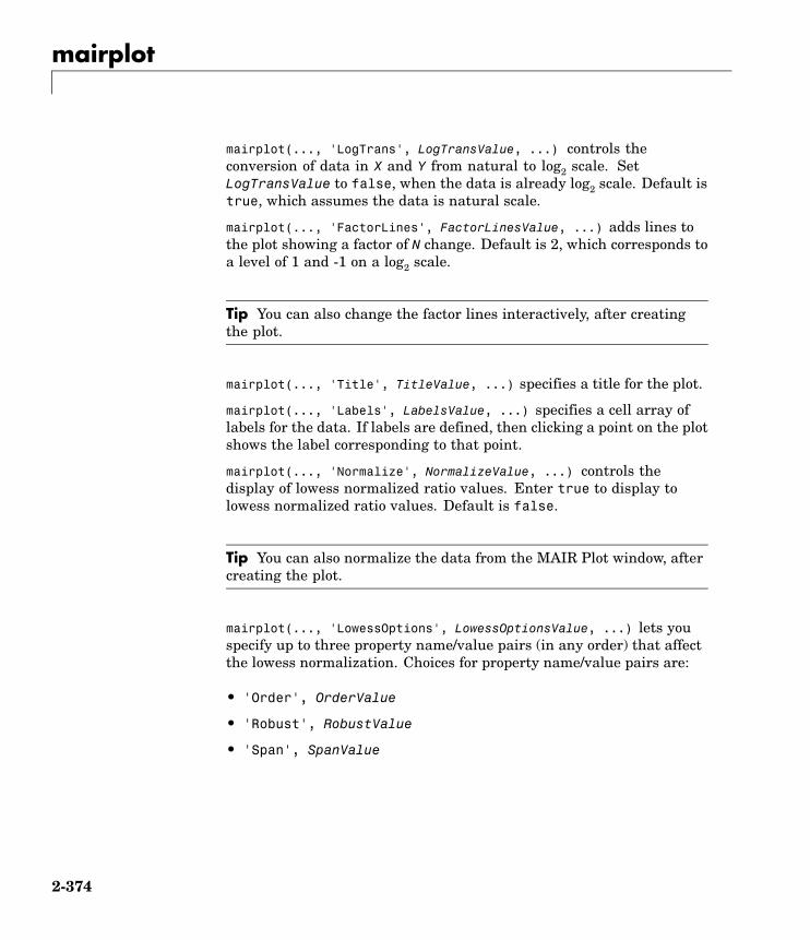
mairplot
mairplot(..., 'LogTrans', LogTransValue, ...) controls theconversion of data in X and Y from natural to log2 scale. SetLogTransValue to false, when the data is already log2 scale. Default istrue, which assumes the data is natural scale.
mairplot(..., 'FactorLines', FactorLinesValue, ...) adds lines tothe plot showing a factor of N change. Default is 2, which corresponds toa level of 1 and -1 on a log2 scale.
Tip You can also change the factor lines interactively, after creatingthe plot.
mairplot(..., 'Title', TitleValue, ...) specifies a title for the plot.
mairplot(..., 'Labels', LabelsValue, ...) specifies a cell array oflabels for the data. If labels are defined, then clicking a point on the plotshows the label corresponding to that point.
mairplot(..., 'Normalize', NormalizeValue, ...) controls thedisplay of lowess normalized ratio values. Enter true to display tolowess normalized ratio values. Default is false.
Tip You can also normalize the data from the MAIR Plot window, aftercreating the plot.
mairplot(..., 'LowessOptions', LowessOptionsValue, ...) lets youspecify up to three property name/value pairs (in any order) that affectthe lowess normalization. Choices for property name/value pairs are:
• 'Order', OrderValue
• 'Robust', RobustValue
• 'Span', SpanValue
2-374
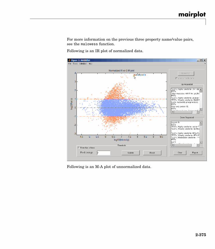
mairplot
For more information on the previous three property name/value pairs,see the malowess function.
Following is an IR plot of normalized data.
Following is an M-A plot of unnormalized data.
2-375
mairplot
The intensity versus ratio scatter plot displays the following:
• log10 (Intensity) versus log2 (Ratio) scatter plot of genes.
• Two horizontal fold change lines at a fold change level of 2, whichcorresponds to a ratio of 1 and –1 on a log2 (Ratio) scale. (Lines willbe at different fold change levels, if you used the 'FactorLines'property.)
• Data points for genes that are considered differentially expressed(outside of the fold change lines) appear in orange.
2-376

mairplot
After you display the intensity versus ratio scatter plot, you caninteractively do the following:
• Adjust the horizontal fold change lines by click-dragging one line orentering a value in the Fold Change text box, then clicking Update.
• Display labels for data points by clicking a data point.
• Select a gene from the Up Regulated or Down Regulated list tohighlight the corresponding data point in the plot. Press and holdCtrl or Shift to select multiple genes.
• Zoom the plot by selecting Tools > Zoom In or Tools > Zoom Out.
• View lists of significantly up-regulated and down-regulated genes,and optionally, export the gene labels and indices to a structure inthe MATLAB workspace by clicking Export.
• Normalize the data by clicking the Normalize button, then selectingwhether to show the normalized plot in a separate window. If youshow the normalized plot in a separate window, the Show smoothcurve check box becomes available in the original (unnormalized)plot.
Note To select different lowess normalization options beforenormalizing, select Tools > Set LOWESS Normalization Options,then select options from the Options dialog box.
Examples 1 Use the gprread function to create a structure containing microarraydata.
maStruct = gprread('mouse_a1wt.gpr');
2 Use the magetfield function to extract the green (cy3) and red (cy5)signals from the structure.
2-377

mairplot
cy3data = magetfield(maStruct,'F635 Median');cy5data = magetfield(maStruct,'F532 Median');
3 Create an intensity versus ratio scatter plot of the cy3 and cy5 data.Normalize the data and add a title and labels:
mairplot(cy3data, cy5data, 'Normalize', true, ...'Title','Normalized R vs G IR plot', ...'Labels', maStruct.Names)
4 Return intensity values and ratios without displaying the plot.
[intensities, ratios] = mairplot(cy3data, cy5data, 'Showplot', false);
References [1] Quackenbush, J. (2002). Microarray Data Normalization andTransformation. Nature Genetics Suppl. 32, 496–501.
[2] Dudoit, S., Yang, Y.H., Callow, M.J., and Speed, T.P. (2002).Statistical Methods for Identifying Differentially Expressed Genesin Replicated cDNA Microarray Experiments. Statistica Sinica 12,111–139.
See Also Bioinformatics Toolbox functions: maboxplot, magetfield,maimage, mainvarsetnorm, maloglog, malowess, manorm, mattest,mavolcanoplot
2-378

maloglog
Purpose Create loglog plot of microarray data
Syntax maloglog(X, Y, 'PropertyName', PropertyValue...)maloglog(..., 'FactorLines', N)maloglog(..., 'Title', TitleValue)maloglog(..., 'Labels', LabelsValues)maloglog(..., 'HandleGraphicsName', HGValue)H = maloglog(...)
ArgumentsX A numeric array of microarray expression values from
a single experimental condition.
Y A numeric array of microarray expression values froma single experimental condition.
N Property to add two lines to the plot showing a factorof N change.
TitleValue A string to use as the title for the plot.
LabelsValue A cell array of labels for the data in X and Y. If youspecify LabelsValue, then clicking a data point in theplot shows the label corresponding to that point.
Description maloglog(X, Y, 'PropertyName', PropertyValue...) creates a loglogscatter plot of X versus Y. X and Y are numeric arrays of microarrayexpression values from two different experimental conditions.
maloglog(..., 'FactorLines', N) adds two lines to the plot showinga factor of N change.
maloglog(..., 'Title', TitleValue) allows you to specify a title forthe plot.
maloglog(..., 'Labels', LabelsValues) allows you to specify a cellarray of labels for the data. If LabelsValues is defined, then clicking adata point in the plot shows the label corresponding to that point.
maloglog(..., 'HandleGraphicsName', HGValue) allows you to passoptional Handle Graphics property name/property value pairs to thefunction.
2-379

maloglog
H = maloglog(...) returns the handle to the plot.
Examples maStruct = gprread('mouse_a1wt.gpr');Red = magetfield(maStruct,'F635 Median');Green = magetfield(maStruct,'F532 Median');maloglog(Red,Green,'title','Red vs Green');% Add factorlines and labelsfiguremaloglog(Red,Green,'title','Red vs Green',...
'FactorLines',2,'LABELS',maStruct.Names);% Now create a normalized plotfiguremaloglog(manorm(Red),manorm(Green),'title',...
'Normalized Red vs Green','FactorLines',2,...'LABELS',maStruct.Names);
See Also Bioinformatics Toolbox functions maboxplot, magetfield,mainvarsetnorm, maimage, mairplot, malowess, manorm, mattest,mavolcanoplot
MATLAB function loglog
2-380

malowess
Purpose Smooth microarray data using Lowess method
Syntax YSmooth = malowess(X, Y)malowess(..., 'PropertyName', PropertyValue,...)malowess(..., 'Order', OrderValue ...)malowess(..., 'Robust', RobustValue ...)malowess(..., 'Span', SpanValue ...)
ArgumentsX, Y Scatter data.
OrderValue Property to select the order of the algorithm. Entereither 1 (linear fit) or 2 (quadratic fit). The defaultorder is 1.
RobustValue Property to select a robust fit. Enter either true orfalse.
SpanValue Property to specify the window size. The defaultvalue is 0.05 (5% of total points in X)
Description YSmooth = malowess(X, Y) smooths scatter data (X, Y) using theLowess smoothing method. The default window size is 5% of the lengthof X.
malowess(..., 'PropertyName', PropertyValue,...) definesoptional properties using property name/value pairs.
malowess(..., 'Order', OrderValue ...) chooses the order of thealgorithm. Note that Curve Fitting Toolbox refers to Lowess smoothingof order 2 as Loess smoothing.
malowess(..., 'Robust', RobustValue ...) uses a robust fit whenRobustValue is set to true. This option can take a long time to calculate.
malowess(..., 'Span', SpanValue ...) modifies the window sizefor the smoothing function. If SpanValue is less than 1, the windowsize is taken to be a fraction of the number of points in the data. IfSpanValue is greater than 1, the window is of size SpanValue.
2-381

malowess
Examples maStruct = gprread('mouse_a1wt.gpr');cy3data = magetfield(maStruct, 'F635 Median');cy5data = magetfield(maStruct, 'F532 Median');[x,y] = mairplot(cy3data, cy5data);drawnowysmooth = malowess(x,y);hold on;plot(x, ysmooth, 'rx')ynorm = y - ysmooth;
See Also Bioinformatics Toolbox functions affyinvarsetnorm, maboxplot,magetfield, maimage, mainvarsetnorm, mairplot, maloglog, manorm,quantilenorm
Statistics Toolbox function robustfit
2-382
manorm
Purpose Normalize microarray data
Syntax XNorm = manorm(X)XNorm = manorm(MAStruct, FieldName)[XNorm, ColVal] = manorm(...)manorm(..., 'Method', MethodValue)manorm(..., 'Extra_Args', Extra_ArgsValue)manorm(..., 'LogData', LogDataValue)manorm(..., 'Percentile', PercentileValue)manorm(..., 'Global', GlobalValue),manorm(..., 'StructureOutput', StructureOutputValue)manorm(..., 'NewColumnName', NewColumnNameValue)
Description XNorm = manorm(X) scales the values in each column of microarraydata (X) by dividing by the mean column intensity.
• X — Microarray data. Enter a vector or matrix.
• XNorm — Normalized microarray data.
XNorm = manorm(MAStruct, FieldName) scales the data for a field(FieldName) for each block or print-tip by dividing each block by themean column intensity. The output is a matrix with each columncorresponding to the normalized data for each block.
• MAStruct — Microarray structure.
[XNorm, ColVal] = manorm(...) returns the values used to normalizethe data.
manorm(..., 'Method', MethodValue) allows you to choose themethod for scaling or centering the data. MethodValue can be 'Mean’(default), 'Median’, 'STD' (standard deviation), 'MAD' (median absolutedeviation), or a function handle. If you pass a function handle, thenthe function should ignore NaNs and must return a single value percolumn of the input data.
2-383

manorm
manorm(..., 'Extra_Args', Extra_ArgsValue) allows you to passextra arguments to the function MethodValue. Extra_ArgsValue mustbe a cell array.
manorm(..., 'LogData', LogDataValue), when LogDataValue istrue, works with log ratio data in which case the mean (or MethodValue)of each column is subtracted from the values in the columns, instead ofdividing the column by the normalizing value.
manorm(..., 'Percentile', PercentileValue) only uses thepercentile (PercentileValue) of the data preventing large outliers fromskewing the normalization. If PercentileValue is a vector containingtwo values, then the range from the PercentileValue(1) percentile tothe PercentileValue(2) percentile is used. The default value is 100,that is to use all the data in the data set.
manorm(..., 'Global', GlobalValue), when GlobalValue istrue, normalizes the values in the data set by the global mean (orMethodValue) of the data, as opposed to normalizing each column orblock of the data independently.
manorm(..., 'StructureOutput', StructureOutputValue), whenStructureOutputValue is true, the input data is a structure returnsthe input structure with an additional data field for the normalizeddata.
manorm(..., 'NewColumnName', NewColumnNameValue), when usingStructureOutput, allows you to specify the name of the column thatis appended to the list of ColumnNames in the structure. The defaultbehavior is to prefix 'Block Normalized' to the FieldName string.
Examples maStruct = gprread('mouse_a1wt.gpr');
% Extract some data of interest.
Red = magetfield(maStruct,'F635 Median');
Green = magetfield(maStruct,'F532 Median');
% Create a log-log plot.
maloglog(Red,Green,'factorlines',true)
% Center the data.
normRed = manorm(Red);
2-384

manorm
normGreen = manorm(Green);
% Create a log-log plot of the centered data.
figure
maloglog(normRed,normGreen,'title','Normalized','factorlines',true)
% Alternatively, you can work directly with the structure
normRedBs = manorm(maStruct,'F635 Median - B635');
normGreenBs = manorm(maStruct,'F532 Median - B532');
% Create a log-log plot of the centered data. This includes some
% zero values so turn off the warning.
figure
w = warning('off','Bioinfo:maloglog:ZeroValues');
warning('off','Bioinfo:maloglog:NegativeValues');
maloglog(normRedBs,normGreenBs,'title',...
'Normalized Background-Subtracted Median Values',...
'factorlines',true)
warning(w);
See Also Bioinformatics Toolbox functions affyinvarsetnorm, maboxplot,magetfield, mainvarsetnorm, mairplot, maloglog, malowess,quantilenorm, rmasummary
2-385
mapcaplot
Purpose Create Principal Component Analysis plot of microarray data
Syntax mapcaplot(Data)mapcaplot(Data, Label)
ArgumentsData Microarray expression profile data.
Label Cell array of strings representing labels for the datapoints.
Description mapcaplot(Data) creates 2-D scatter plots of principal components ofthe array Data.
mapcaplot(Data, Label) uses the elements of the cell array of stringsLabel, instead of the row numbers, to label the data points.
2-386

mapcaplot
2-387

mapcaplot
Once you plot the principal components, you can:
• Select principal components for the x and y axes from the drop-downlist boxes below each scatter plot.
• Click a data point to display its label.
• Select a subset of data points by click-dragging a box aroundthem. This will highlight the points in the selected region and thecorresponding points in the other axes. The labels of the selecteddata points appear in the list box.
• Select a label in the list box to highlight the corresponding datapoint in the plot. Press and hold Ctrl or Shift to select multipledata points.
• Export the gene labels and indices to a structure in the MATLABworkspace by clicking Export.
Examples load filteredyeastdatamapcaplot(yeastvalues, genes)
See Also Bioinformatics Toolbox functions: clustergram, mattest,mavolcanoplot
Statistics Toolbox function: princomp
2-388
mattest
Purpose Perform two-tailed t-test to evaluate differential expression of genesfrom two experimental conditions or phenotypes
Syntax PValues = mattest(DataX, DataY)[PValues, TScores] = mattest(DataX, DataY)[PValues, TScores, DFs] = mattest(DataX, DataY)... = mattest(..., 'Permute', PermuteValue, ...)... = mattest(..., 'Showhist', ShowhistValue, ...)... = mattest(..., 'Showplot', ShowplotValue, ...)... = mattest(..., 'Labels', LabelsValue, ...)
ArgumentsDataX, DataY Matrices of gene expression values where each
row corresponds to a gene and each columncorresponds to a replicate. DataX and DataY musthave the same number of rows and are assumedto be normally distributed in each class withequal variances.
DataX contains data from one experimentalcondition and DataY contains data from adifferent experimental condition. For example, ina two-color microarray experiment, DataX couldbe cy3 intensity values and DataY could be cy5intensity values.
PermuteValue Controls whether permutation tests are run,and if so, how many. Choices are true, false(default), or any integer greater than 2. If set totrue, the number of permutations is 1000.
ShowhistValue Controls the display of histograms of t-scoredistributions and p-value distributions. Choicesare true or false (default).
2-389

mattest
ShowplotValue Controls the display of a normal t-score quantileplot. Choices are true or false (default). In thet-score quantile plot, data points with t-scores> (1 - 1/(2N)) or < 1/(2N) display with redcircles. N is the total number of genes.
LabelsValue Cell array of labels (typically gene names orprobe set IDs) for each row in DataX and DataY.The labels display if you click a data point in thet-score quantile plot.
ReturnValues
PValues Column vector of p-values for each gene in DataXand DataY.
TScores Column vector of t-scores for each gene in DataXand DataY.
DFs Column vector containing the degree of freedom foreach gene in DataX and DataY.
Description PValues = mattest(DataX, DataY) compares the gene expressionprofiles in DataX and DataY and returns a p-value for each gene. DataXand DataY are matrices of gene expression values, in which each rowcorresponds to a gene, and each column corresponds to a replicate.DataX contains data from one experimental condition and DataYcontains data from another experimental condition. DataX and DataYmust have the same number of rows and are assumed to be normallydistributed in each class with equal variances. PValues is a columnvector of p-values for each gene.
[PValues, TScores] = mattest(DataX, DataY) also returns a t-scorefor each gene in DataX and DataY. TScores is a column vector of t-scoresfor each gene.
2-390

mattest
[PValues, TScores, DFs] = mattest(DataX, DataY) also returnsDFs, a column vector containing the degree of freedom for each geneacross both data sets, DataX and DataY.
... = mattest(..., 'PropertyName', PropertyValue, ...) callsmattest with optional properties that use property name/propertyvalue pairs. You can specify one or more properties in any order. EachPropertyName must be enclosed in single quotation marks and is caseinsensitive. These property name/property value pairs are as follows:
... = mattest(..., 'Permute', PermuteValue, ...) controlswhether permutation tests are run, and if so, how many. PermuteValuecan be true, false (default), or any integer greater than 2. If set totrue, the number of permutations is 1000.
... = mattest(..., 'Showhist', ShowhistValue, ...) controlsthe display of histograms of t-score distributions and p-valuedistributions. When ShowhistValue is true, mattest displayshistograms. Default is false.
2-391
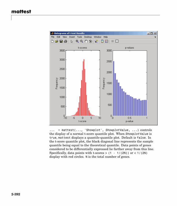
mattest
... = mattest(..., 'Showplot', ShowplotValue, ...) controlsthe display of a normal t-score quantile plot. When ShowplotValue istrue, mattest displays a quantile-quantile plot. Default is false. Inthe t-score quantile plot, the black diagonal line represents the samplequantile being equal to the theoretical quantile. Data points of genesconsidered to be differentially expressed lie farther away from this line.Specifically, data points with t-scores > (1 - 1/(2N)) or < 1/(2N)display with red circles. N is the total number of genes.
2-392

mattest
... = mattest(..., 'Labels', LabelsValue, ...) controls thedisplay of labels when you click a data point in the t-score quantile plot.LabelsValue is a cell array of labels (typically gene names or probe setIDs) for each row in DataX and DataY.
Examples 1 Load the MAT file, included with Bioinformatics Toolbox, thatcontains Affymetrix data from a prostate cancer study, specificallyprobe intensity data from Affymetrix HG-U133A GeneChiparrays. The two variables in the MAT file, dependentData andindependentData, are two matrices of gene expression values fromtwo experimental conditions.
2-393
mattest
load prostatecancerexpdata
2 Calculate the p-values and t-scores for the gene expression values inthe two matrices and display a normal t-score quantile plot.
[pvalues,tscores] = mattest(dependentData, independentData,...'showplot',true);
3 Calculate the p-values and t-scores again using permutationtests (1000 permutations) and displaying histograms of t-scoredistributions and p-value distributions.
[pvalues,tscores] = mattest(dependentData,independentData,...'permute',true,'showhist',true,...'showplot',true);
The prostatecancerexpdata.mat file used in this example containsdata from Best et al., 2005.
References [1] Huber, W., von Heydebreck, A., Sültmann, H., Poustka, A., andVingron, M. (2002). Variance stabilization applied to microarraydata calibration and to the quantification of differential expression.Bioinformatics 18 Suppl1, S96–S104.
[2] Best, C.J.M., Gillespie, J.W., Yi, Y., Chandramouli, G.V.R.,Perlmutter, M.A., Gathright, Y., Erickson, H.S., Georgevich, L., Tangrea,M.A., Duray, P.H., Gonzalez, S., Velasco, A., Linehan, W.M., Matusik,R.J., Price, D.K., Figg, W.D., Emmert-Buck, M.R., and Chuaqui, R.F.(2005). Molecular alterations in primary prostate cancer after androgenablation therapy. Clinical Cancer Research 11, 6823–6834.
See Also Bioinformatics Toolbox functions: maboxplot, mafdr, mainvarsetnorm,mairplot, maloglog, malowess, manorm, mavolcanoplot, rmasummary
2-394

mavolcanoplot
Purpose Create significance versus gene expression ratio (fold change) scatterplot of microarray data
Syntax mavolcanoplot(DataX, DataY, PValues)SigStructure = mavolcanoplot(DataX, DataY, PValues)... mavolcanoplot(..., 'Labels', LabelsValue, ...)... mavolcanoplot(..., 'LogTrans', LogTransValue, ...)... mavolcanoplot(..., 'PCutoff', PCutoffValue, ...)... mavolcanoplot(..., 'Foldchange', FoldchangeValue, ...)
ArgumentsDataX Matrix or vector of gene expression values
from a single experimental condition. IfDataX is a matrix, each row is a gene,each column is a sample, and an averageexpression value is calculated for eachgene.
Note If the values in DataX are naturalscale, use the LogTrans property toconvert them to log 2 scale.
DataY Matrix or vector of gene expression valuesfrom a single experimental condition. If amatrix, each row is a gene, each columnis a sample, and an average expressionvalue is calculated for each gene.
Note If the values in DataY are naturalscale, use the LogTrans property toconvert them to log 2 scale.
2-395

mavolcanoplot
PValues Vector of p-values for each gene in datasets from two different experimentalconditions.
LabelsValue Cell array of labels (typically gene namesor probe set IDs) for the data. Aftercreating the plot, you can click a datapoint to display the label associated withit. If you do not provide a LabelsValue,data points are labeled with row numbersfrom DataX and DataY.
LogTransValue Property to control the conversion of datain DataX and DataY from natural scale tolog 2 scale. Enter true to convert data tolog 2 scale, or false. Default is false,which assumes data is already log 2 scale.
2-396
mavolcanoplot
PCutoffValue Lets you specify a cutoff p-value todefine data points that are statisticallysignificant. This value is displayedgraphically as a horizontal line on theplot. Default is 0.05, which is equivalentto 1.3010 on the –log10 (p-value) scale.
Note You can also change the p-valuecutoff interactively after creating the plot.
FoldchangeValue Lets you specify a ratio fold change todefine data points that are differentiallyexpressed. Default is 2, which correspondsto a ratio of 1 and –1 on a log2 (ratio) scale.
Note You can also change the fold changeinteractively after creating the plot.
Description mavolcanoplot(DataX, DataY, PValues) creates a scatter plot of geneexpression data, plotting significance versus fold change of geneexpression ratios. It uses the average gene expression values from twodata sets, DataX and DataY, for each gene in the data sets. It plotssignificance as the –log10 (p-value) from the vector, PValues. DataX andDataY can be vectors or matrices.
SigStructure = mavolcanoplot(DataX, DataY, PValues) returnsa structure containing information for genes that are considered to beboth statistically significant (above the p-value cutoff) and significantlydifferentially expressed (outside of the fold change values). The fieldswithin SigStructure are sorted by p-value and include:
• Name
• PCutoff
2-397

mavolcanoplot
• FCThreshold
• GeneLabels
• PValues
• FoldChanges
... mavolcanoplot(..., 'PropertyName', PropertyValue, ...)defines optional properties that use property name/value pairs in anyorder. These property name/value pairs are as follows:
... mavolcanoplot(..., 'Labels', LabelsValue, ...) lets you providea cell array of labels (typically gene names or probe set IDs) for the data.After creating the plot, you can click a data point to display the labelassociated with it. If you do not provide a LabelsValue, data points arelabeled with row numbers from DataX and DataY.
... mavolcanoplot(..., 'LogTrans', LogTransValue, ...) controlsthe conversion of data from DataX and DataY to log2 scale. WhenLogTransValue is true, mavolcanoplot converts data from natural tolog2 scale. Default is false, which assumes the data is already log2scale.
... mavolcanoplot(..., 'PCutoff', PCutoffValue, ...) lets youspecify a p-value cutoff to define data points that are statisticallysignificant. This value displays graphically as a horizontal line onthe plot. Default is 0.05, which is equivalent to 1.3010 on the –log10(p-value) scale.
Note You can also change the p-value cutoff interactively after creatingthe plot.
... mavolcanoplot(..., 'Foldchange', FoldchangeValue, ...)lets you specify a ratio fold change to define data points that aredifferentially expressed. Fold changes display graphically as two
2-398
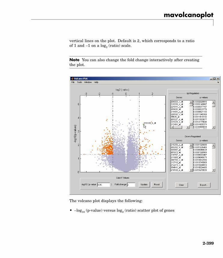
mavolcanoplot
vertical lines on the plot. Default is 2, which corresponds to a ratioof 1 and –1 on a log2 (ratio) scale.
Note You can also change the fold change interactively after creatingthe plot.
The volcano plot displays the following:
• –log10 (p-value) versus log2 (ratio) scatter plot of genes
2-399

mavolcanoplot
• Two vertical fold change lines at a fold change level of 2, whichcorresponds to a ratio of 1 and –1 on a log2 (ratio) scale. (Lines willbe at different fold change levels, if you used the 'Foldchange'property.)
• One horizontal line at the 0.05 p-value level, which is equivalent to1.3010 on the –log10 (p-value) scale. (The line will be at a differentp-value level, if you used the 'PCutoff' property.)
• Data points for genes that are considered both statistically significant(above the p-value line) and differentially expressed (outside of thefold changes lines) appear in orange.
After you display the volcano scatter plot, you can interactively:
• Adjust the vertical fold change lines by click-dragging one line orentering a value in the Fold Change text box.
• Adjust the horizontal p-value cutoff line by click-dragging or enteringa value in the p-value Cutoff text box.
• Display labels for data points by clicking a data point.
• Select a gene from the Up Regulated or Down Regulated list tohighlight the corresponding data point in the plot. Press and holdCtrl or Shift to select multiple genes.
• Zoom the plot by selecting Tools > Zoom In or Tools > Zoom Out.
• View lists of significantly up-regulated and down-regulated genesand their associated p-values, and optionally, export the labels,p-values, and fold changes to a structure in the MATLAB Workspaceby clicking Export.
Examples 1 Load a MAT file, included with Bioinformatics Toolbox, whichcontains Affymetrix data variables, including dependentData and
2-400
mavolcanoplot
independentData, two matrices of gene expression values from twoexperimental conditions.
load prostatecancerexpdata
2 Use the mattest function to calculate p-values for the geneexpression values in the two matrices.
pvalues = mattest(dependentData, independentData);
3 Using the two matrices, the pvalues calculated by mattest, and theprobesetIDs column vector of labels provided, use mavolcanoplot tocreate a significance versus gene expression ratio scatter plot of themicroarray data from the two experimental conditions.
mavolcanoplot(dependentData, independentData, pvalues,...'Labels', probesetIDs)
The prostatecancerexpdata.mat file used in the previous examplecontains data from Best et al., 2005.
References [1] Cui, X., Churchill, G.A. (2003). Statistical tests for differentialexpression in cDNA microarray experiments. Genome Biology 4, 210.
[2] Best, C.J.M., Gillespie, J.W., Yi, Y., Chandramouli, G.V.R.,Perlmutter, M.A., Gathright, Y., Erickson, H.S., Georgevich, L., Tangrea,M.A., Duray, P.H., Gonzalez, S., Velasco, A., Linehan, W.M., Matusik,R.J., Price, D.K., Figg, W.D., Emmert-Buck, M.R., and Chuaqui, R.F.(2005). Molecular alterations in primary prostate cancer after androgenablation therapy. Clinical Cancer Research 11, 6823–6834.
See Also Bioinformatics Toolbox functions: maboxplot, maimage,mainvarsetnorm, mairplot, maloglog, malowess, manorm, mapcaplot,mattest
2-401

molweight
Purpose Calculate molecular weight of amino acid sequence
Syntax molweight(SeqAA)
ArgumentsSeqAA Amino acid sequence. Enter a character string or a
vector of integers from the Amino Acid Lookup Table onpage 2-42. Examples: 'ARN', [1 2 3]. You can alsoenter a structure with the field Sequence.
Description molweight(SeqAA) calculates the molecular weight for the amino acidsequence SeqAA.
Examples 1 Get an amino acid sequence from the NCBI Genpept Database
rhodopsin = getgenpept('NP_000530');
2 Calculate the molecular weight of the sequence.
rhodopsinMW = molweight(rhodopsin)
rhodopsinMW =
3.8892e+004
See Also Bioinformatics Toolbox functions: aacount, atomiccomp, isoelectric,proteinplot
2-402
molviewer
Purpose Display and manipulate 3-D molecule structure
Syntax molviewermolviewer(File)molviewer(pdbID)molviewer(pdbStruct)FigureHandle = molviewer(...)
2-403

molviewer
ArgumentsFile String specifying one of the following:
• File name of a file on the MATLAB search path orin the MATLAB Current Directory
• Path and file name
• URL pointing to a file (URL must begin with aprotocol such as http://, ftp://, or file://)
The referenced file is a molecule model file, such as aProtein Data Bank (PDB)-formatted file (ASCII textfile). Valid file types include:
• PDB
• MOL (MDL)
• SDF
• XYZ
• SMOL
• JVXL
• CIF/mmCIF
pdbID String specifying a unique identifier for a proteinstructure record in the PDB database.
Note Each structure in the PDB database isrepresented by a four-character alphanumericidentifier. For example, 4hhb is the identifier forhemoglobin.
pdbStruct A structure containing a field for each PDB record,such as returned by the getpdb or pdbread function.
2-404

molviewer
ReturnValues FigureHandle Figure handle to a Molecule Viewer window.
Description molviewer opens a blank Molecule Viewer window. You can display3-D molecular structures by selecting File > Open, File > Load PDBID, or File > Open URL.
molviewer(File) reads the data in a molecule model file, File, andopens a Molecule Viewer window displaying the 3-D molecular structurefor viewing and manipulation.
molviewer(pdbID) retrieves the data for a protein structure record,pdbID, from the PDB database and opens a Molecule Viewer windowdisplaying the 3-D molecular structure for viewing and manipulation.
molviewer(pdbStruct) reads the data from pdbStruct, a structurecontaining a field for each PDB record, and opens a MoleculeViewer window displaying a 3-D molecular structure for viewing andmanipulation.
FigureHandle = molviewer(...) returns the figure handle to theMolecule Viewer window.
Tip You can pass the FigureHandle to the evalrasmolscript function,which sends RasMol script commands to the Molecule Viewer window.
Tip If you receive any errors related to memory or Java heap space, tryincreasing your Java heap space as described at:
http://www.mathworks.com/support/solutions/data/1-18I2C.html
2-405

molviewer
2-406

molviewer
After displaying the 3-D molecule structure, you can:
• Click-drag the molecule to spin, rotate, and view it from differentangles.
• Hover the mouse over a subcomponent of the molecule to display anidentification label for it.
• Zoom the plot by turning the mouse scroll wheel or clicking thefollowing buttons:
or
• Spin the molecule by clicking .
• Change the background color between black and white by clicking
.
• Reset the molecule position by clicking .
• Show or hide the Control Panel by clicking .
• Manipulate and annotate the 3-D structure by selecting options inthe Control Panel or by right-clicking to select commands:
2-407

molviewer
• Display the RasMol Scripts console by clicking .
2-408
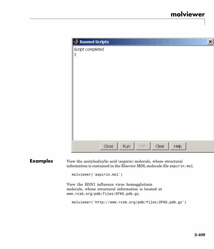
molviewer
Examples View the acetylsalicylic acid (aspirin) molecule, whose structuralinformation is contained in the Elsevier MDL molecule file aspirin.mol.
molviewer('aspirin.mol')
View the H5N1 influenza virus hemagglutininmolecule, whose structural information is located atwww.rcsb.org/pdb/files/2FK0.pdb.gz.
molviewer('http://www.rcsb.org/pdb/files/2FK0.pdb.gz')
2-409

molviewer
View the molecule with a PDB identifier of 2DHB.
molviewer('2DHB')
View the molecule with a PDB identifier of 4hhb, and create a figurehandle for the molecule viewer.
FH = molviewer('4hhb')
Use the getpdb function to retrieve protein structure data from thePDB database and create a MATLAB structure. Then view the proteinmolecule.
pdbstruct = getpdb('1vqx')molviewer(pdbstruct)
See Also Bioinformatics Toolbox functions: evalrasmolscript, getpdb, pdbread,pdbwrite
2-410
msalign
Purpose Align peaks in mass spectrum to reference peaks
Syntax IntensitiesOut = msalign(MZ, Intensities, RefMZ)... = msalign(..., 'Weights', WeightsValue, ...)... = msalign(..., 'Range', RangeValue, ...)... = msalign(..., 'WidthOfPulses',WidthOfPulsesValue, ...)... = msalign(..., 'WindowSizeRatio', WindowSizeRatioValue,
...)... = msalign(..., 'Iterations', IterationsValue, ...)... = msalign(..., 'GridSteps', GridStepsValue, ...)... = msalign(..., 'SearchSpace', SearchSpaceValue, ...)... = msalign(..., 'ShowPlot', ShowPlotValue, ...)[IntensitiesOut, RefMZOut] = msalign(...,'Group', GroupValue,
...)
Arguments MZ Vector of mass/charge (m/z) values for aspectrum or set of spectra. The numberof elements in the vector equals n or thenumber of rows in the matrix Intensities.
Intensities Either of the following:• Column vector of intensity values for a
spectrum, where each row corresponds toan m/z value.
• Matrix of intensity values for a set of massspectra that share the same m/z range,where each row corresponds to an m/zvalue, and each column corresponds to aspectrum.
The number of rows equals n or the numberof elements in vector MZ.
2-411

msalign
RefMZ Vector of m/z values of known referencemasses in a sample spectrum.
Tip For reference peaks, selectcompounds that do not undergo structuraltransformation, such as phosphorylation.Doing so will increase the accuracy of youralignment and allow you to detect compoundsthat do exhibit structural transformationsamong the sample spectra.
WeightsValue Vector of positive values, with the samenumber of elements as RefMZ. The defaultvector is ones(size(RefMZ)).
RangeValue Two-element vector, in which the firstelement is negative and the second elementis positive, that specifies the lower and upperlimits of a range, in m/z units, relative toeach peak. No peak will shift beyond theselimits. Default is [-100 100].
WidthOfPulsesValue Positive value that specifies the width,in m/z units, for all the Gaussian pulsesused to build the correlating syntheticspectrum. The point of the peak wherethe Gaussian pulse reaches 60.65% of itsmaximum is set to the width specified byWidthOfPulsesValue. Default is 10.
2-412
msalign
WindowSizeRatioValue Positive value that specifies a scalingfactor that determines the size of thewindow around every alignment peak.The synthetic spectrum is comparedto the sample spectrum only withinthese regions, which saves computationtime. The size of the window is givenin m/z units by WidthOfPulsesValue *WindowSizeRatioValue. Default is 2.5,which means at the limits of the window, theGaussian pulses have a value of 4.39% oftheir maximum.
IterationsValue Positive integer that specifies the number ofrefining iterations. At every iteration, thesearch grid is scaled down to improve theestimates. Default is 5.
GridStepsValue Positive integer that specifies the numberof steps for the search grid. At everyiteration, the search area is divided byGridStepsValue^2. Default is 20.
SearchSpaceValue String that specifies the type of search space.Choices are:• 'regular' — Default. Evenly spaced
lattice.
• 'latin' — Random Latin hypercube withGridStepsValue^2 samples.
2-413

msalign
ShowPlotValue Controls the display of a plot of an originaland aligned spectrum over the referencemasses specified by RefMZ. Choices are true,false, or I, an integer specifying the indexof a spectrum in Intensities. If set to true,the first spectrum in Intensities is plotted.Default is:
• false — When return values are specified.
• true — When return values are notspecified.
GroupValue Controls the creation of RefMZOut, a newvector of m/z values to be used as referencemasses for aligning the peaks. This vectoris created by adjusting the values in RefMZ,based on the sample data from multiplespectra in Intensities, such that theoverall shifting and scaling of the peaksis minimized. Choices are true or false(default).
Tip Set GroupValue to true only ifIntensities contains data for a largenumber of spectra, and you are not confidentof the m/z values used for your referencepeaks in RefMZ. Leave GroupValue set tofalse if you are confident of the m/z valuesused for your reference peaks in RefMZ.
2-414
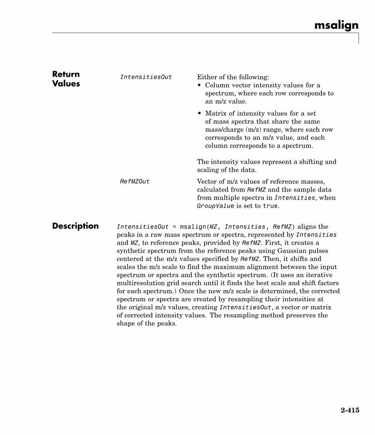
msalign
ReturnValues
IntensitiesOut Either of the following:• Column vector intensity values for a
spectrum, where each row corresponds toan m/z value.
• Matrix of intensity values for a setof mass spectra that share the samemass/charge (m/z) range, where each rowcorresponds to an m/z value, and eachcolumn corresponds to a spectrum.
The intensity values represent a shifting andscaling of the data.
RefMZOut Vector of m/z values of reference masses,calculated from RefMZ and the sample datafrom multiple spectra in Intensities, whenGroupValue is set to true.
Description IntensitiesOut = msalign(MZ, Intensities, RefMZ) aligns thepeaks in a raw mass spectrum or spectra, represented by Intensitiesand MZ, to reference peaks, provided by RefMZ. First, it creates asynthetic spectrum from the reference peaks using Gaussian pulsescentered at the m/z values specified by RefMZ. Then, it shifts andscales the m/z scale to find the maximum alignment between the inputspectrum or spectra and the synthetic spectrum. (It uses an iterativemultiresolution grid search until it finds the best scale and shift factorsfor each spectrum.) Once the new m/z scale is determined, the correctedspectrum or spectra are created by resampling their intensities atthe original m/z values, creating IntensitiesOut, a vector or matrixof corrected intensity values. The resampling method preserves theshape of the peaks.
2-415
msalign
Note The msalign function works best with three to five referencepeaks (marker masses) that you know will appear in the spectrum.If you use a single reference peak (internal standard), there isa possibility of aligning sample peaks to the incorrect referencepeaks as msalign both scales and shifts the MZ vector. If using asingle reference peak, you might need to only shift the MZ vector.To do this, use IntensitiesOut = interp1(MZ, Intensities,MZ-(ReferenceMass-ExperimentalMass). For more information, seeAligning Mass Spectrum with One Reference Peak on page 2-421.
... = msalign(..., 'PropertyName', PropertyValue, ...) callsmsalign with optional properties that use property name/propertyvalue pairs. You can specify one or more properties in any order. EachPropertyName must be enclosed in single quotation marks and is caseinsensitive. These property name/property value pairs are as follows:
... = msalign(..., 'Weights', WeightsValue, ...) specifiesthe relative weight for each mass in RefMZ, the vector of reference m/zvalues. WeightsValue is a vector of positive values, with the samenumber of elements as RefMZ. The default vector is ones(size(RefMZ)),which means each reference peak is weighted equally, so that moreintense reference peaks have a greater effect in the alignmentalgorithm. If you have a less intense reference peak, you can increaseits weight to emphasize it more in the alignment algorithm.
... = msalign(..., 'Range', RangeValue, ...) specifies thelower and upper limits of the range, in m/z units, relative to each peak.No peak will shift beyond these limits. RangeValue is a two-elementvector, in which the first element is negative and the second element ispositive. Default is [-100 100].
2-416
msalign
Note Use these values to tune the robustness of the algorithm. Ideally,you should keep the range within the maximum expected shift. If youtry to correct larger shifts by increasing the limits, you increase thepossibility of picking incorrect peaks to align to the reference masses.
... = msalign(..., 'WidthOfPulses', WidthOfPulsesValue,
...) specifies the width, in m/z units, for all the Gaussian pulses usedto build the correlating synthetic spectrum. The point of the peakwhere the Gaussian pulse reaches 60.65% of its maximum is set tothe width specified by WidthOfPulsesValue. Choices are any positivevalue. Default is 10. WidthOfPulsesValue may also be a functionhandle. The function is evaluated at the respective m/z values andreturns a variable width for the pulses. Its evaluation should givereasonable values between 0 and max(abs(Range)); otherwise, thefunction returns an error.
Note Tuning the spread of the Gaussian pulses controls a tradeoffbetween robustness (wider pulses) and precision (narrower pulses).However, the spread of the pulses is unrelated to the shape of theobserved peaks in the spectrum. The purpose of the pulse spread is todrive the optimization algorithm.
... = msalign(..., 'WindowSizeRatio',WindowSizeRatioValue, ...) specifies a scaling factorthat determines the size of the window around every alignment peak.The synthetic spectrum is compared to the sample spectrum only withinthese regions, which saves computation time. The size of the window isgiven in m/z units by WidthOfPulsesValue * WindowSizeRatioValue.Choices are any positive value. Default is 2.5, which means at thelimits of the window, the Gaussian pulses have a value of 4.39% oftheir maximum.
2-417

msalign
... = msalign(..., 'Iterations', IterationsValue, ...)specifies the number of refining iterations. At every iteration, thesearch grid is scaled down to improve the estimates. Choices are anypositive integer. Default is 5.
... = msalign(..., 'GridSteps', GridStepsValue, ...)specifies the number of steps for the search grid. At every iteration, thesearch area is divided by GridStepsValue^2. Choices are any positiveinteger. Default is 20.
... = msalign(..., 'SearchSpace', SearchSpaceValue, ...)specifies the type of search space. Choices are:
• 'regular' — Default. Evenly spaced lattice.
• 'latin' — Random Latin hypercube with GridStepsValue^2samples.
... = msalign(..., 'ShowPlot', ShowPlotValue, ...) controlsthe display of a plot of an original and aligned spectrum over thereference masses specified by RefMZ. Choices are true, false, or I, aninteger specifying the index of a spectrum in Intensities. If set totrue, the first spectrum in Intensities is plotted. Default is:
• false — When return values are specified.
• true — When return values are not specified.
[IntensitiesOut, RefMZOut] = msalign(...,'Group', GroupValue, ...) controls the creation of RefMZOut, a newvector of m/z values to be used as reference masses for aligning thepeaks. This vector is created by adjusting the values in RefMZ, basedon the sample data from multiple spectra in Intensities, such thatthe overall shifting and scaling of the peaks is minimized. Choices aretrue or false (default).
2-418
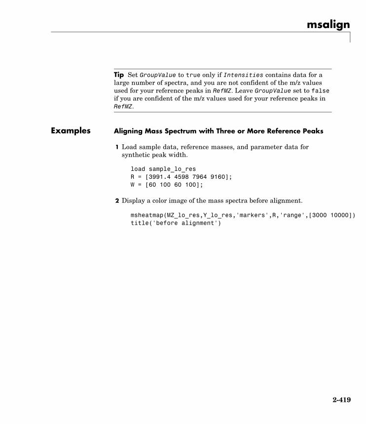
msalign
Tip Set GroupValue to true only if Intensities contains data for alarge number of spectra, and you are not confident of the m/z valuesused for your reference peaks in RefMZ. Leave GroupValue set to falseif you are confident of the m/z values used for your reference peaks inRefMZ.
Examples Aligning Mass Spectrum with Three or More Reference Peaks
1 Load sample data, reference masses, and parameter data forsynthetic peak width.
load sample_lo_resR = [3991.4 4598 7964 9160];W = [60 100 60 100];
2 Display a color image of the mass spectra before alignment.
msheatmap(MZ_lo_res,Y_lo_res,'markers',R,'range',[3000 10000])title('before alignment')
2-419
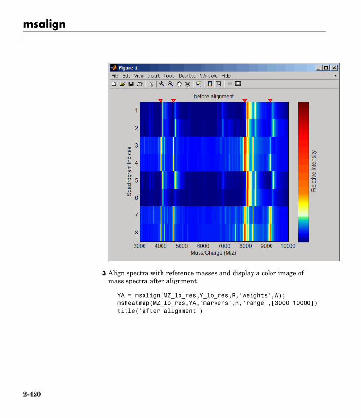
msalign
3 Align spectra with reference masses and display a color image ofmass spectra after alignment.
YA = msalign(MZ_lo_res,Y_lo_res,R,'weights',W);msheatmap(MZ_lo_res,YA,'markers',R,'range',[3000 10000])title('after alignment')
2-420

msalign
Aligning Mass Spectrum with One Reference Peak
It is not recommended to use the msalign function if you have onlyone reference peak. Instead, use the following procedure, which shiftsthe MZ vector, but does not scale it.
1 Load sample data and view the first sample spectrum.
load sample_lo_resMZ = MZ_lo_res;Y = Y_lo_res(:,1);
2-421
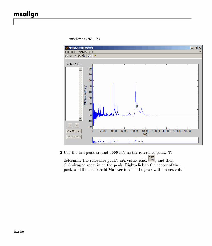
msalign
msviewer(MZ, Y)
2 Use the tall peak around 4000 m/z as the reference peak. To
determine the reference peak’s m/z value, click , and thenclick-drag to zoom in on the peak. Right-click in the center of thepeak, and then click Add Marker to label the peak with its m/z value.
2-422

msalign
3 Shift a spectrum by the difference between RP, the known referencemass of 4000 m/z, and SP, the experimental mass of 4051.14 m/z.
RP = 4000;SP = 4051.14;YOut = interp1(MZ, Y, MZ-(RP-SP));
4 Plot the original spectrum in red and the shifted spectrum in blueand zoom in on the reference peak.
plot(MZ,Y,'r',MZ,YOut,'b:')xlabel('Mass/Charge (M/Z)')ylabel('Relative Intensity')
2-423
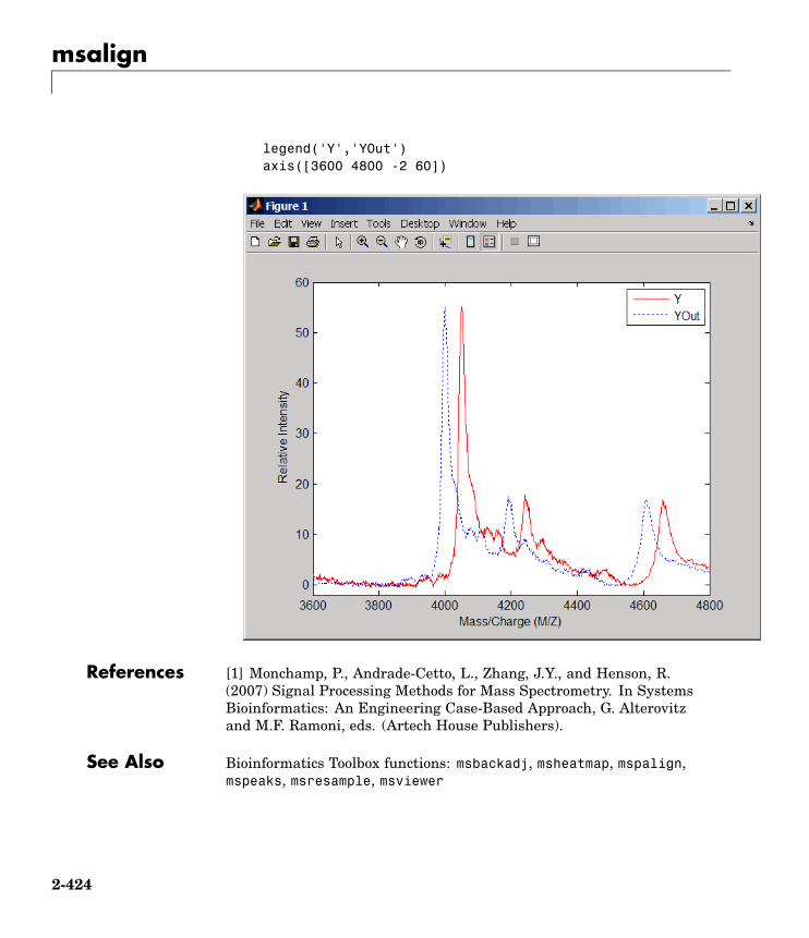
msalign
legend('Y','YOut')axis([3600 4800 -2 60])
References [1] Monchamp, P., Andrade-Cetto, L., Zhang, J.Y., and Henson, R.(2007) Signal Processing Methods for Mass Spectrometry. In SystemsBioinformatics: An Engineering Case-Based Approach, G. Alterovitzand M.F. Ramoni, eds. (Artech House Publishers).
See Also Bioinformatics Toolbox functions: msbackadj, msheatmap, mspalign,mspeaks, msresample, msviewer
2-424

msbackadj
Purpose Correct baseline of mass spectrum
Syntax Yout = msbackadj(MZ, Y)msbackadj(..., 'PropertyName', PropertyValue,...)msbackadj(..., 'WindowSize', WindowSizeValue)msbackadj(..., 'StepSize', StepSizeValue)msbackadj(..., 'RegressionMethod', RegressionMethodValue)msbackadj(..., 'EstimationMethod', EstimationMethodValue)msbackadj(..., 'SmoothMethod', SmoothMethodValue)msbackadj(..., 'QuantileValue', QuantileValueValue)msbackadj(..., 'PreserveHeights', PreserveHeightsValue)msbackadj(..., 'ShowPlot', ShowPlotValue)
ArgumentsMZ Range of mass/charge ions. Enter a vector with the
range of ions in the spectra.
Y Ion intensity vector with the same length as themass/charge vector (MZ). Y can also be a matrix withseveral spectra that share the same mass/charge (MZ)range.
Description Yout = msbackadj(MZ, Y) adjusts the variable baseline of a raw massspectrum by following three steps:
1 Estimates the baseline within multiple shifted windows of width200 m/z
2 Regresses the varying baseline to the window points using a splineapproximation
3 Adjusts the baseline of the spectrum (Y)
msbackadj(..., 'PropertyName', PropertyValue,...) definesoptional properties using property name/value pairs.
2-425
msbackadj
msbackadj(..., 'WindowSize', WindowSizeValue) specifies thewidth for the shifting window. WindowSizeValue can also be a functionhandler. The function is evaluated at the respective MZ values andreturns a variable width for the windows. This option is useful for caseswhere the resolution of the signal is dissimilar at different regions ofthe spectrogram. The default value is 200 (baseline point estimated forwindows with a width of 200 m/z).
Note The result of this algorithm depends on carefully choosing thewindow size and the step size. Consider the width of your peaks inthe spectrum and the presence of possible drifts. If you have widerpeaks towards the end of the spectrum, you may want to use variableparameters.
msbackadj(..., 'StepSize', StepSizeValue)specifies the steps forthe shifting window. The default value is 200 m/z (baseline point isestimated for windows placed every 200 m/z). StepSizeValue may alsobe a function handle. The function is evaluated at the respective m/zvalues and returns the distance between adjacent windows.
msbackadj(..., 'RegressionMethod', RegressionMethodValue)specifies the method to regress the window estimated points to a softcurve. Enter 'pchip' (shape-preserving piecewise cubic interpolation),'linear'(linear interpolation), or 'spline'(spline interpolation). Thedefault value is 'pchip'.
msbackadj(..., 'EstimationMethod', EstimationMethodValue)specifies the method for finding the likely baseline value in everywindow. Enter 'quantile' (quantile value is set to 10%) or 'em'(assumes a doubly stochastic model). With em, every sample isthe independent and identically distributed (i.i.d.) draw of any oftwo normal distributed classes (background or peaks). Becausethe class label is hidden, the distributions are estimated with anExpectation-Maximization algorithm. The ultimate baseline value isthe mean of the background class.
2-426
msbackadj
msbackadj(..., 'SmoothMethod', SmoothMethodValue) specifies themethod for smoothing the curve of estimated points and eliminatingthe effects of possible outliers. Enter 'none', 'lowess' (linear fit),'loess' (quadratic fit), 'rlowess' (robust linear), or 'rloess' ( robustquadratic fit). Default value is 'none'.
msbackadj(..., 'QuantileValue', QuantileValueValue) specifiesthe quantile value. The default value is 0.10.
msbackadj(..., 'PreserveHeights', PreserveHeightsValue),when PreserveHeightsValue is true, sets the baseline subtractionmode to preserve the height of the tallest peak in the signal. The defaultvalue is false and peak heights are not preserved.
msbackadj(..., 'ShowPlot', ShowPlotValue) plots the baselineestimated points, the regressed baseline, and the original spectrum.When msbackadj is called without output arguments, the spectra areplotted unless ShowPlotValue is false. When ShowPlotValue is true,only the first spectrum in Y is plotted. ShowPlotValue can also containan index to one of the spectra in Y.
Example 1 Load sample data.
load sample_lo_res
2 Adjust the baseline for a group of spectra and show only the thirdspectrum and its estimated background.
YB = msbackadj(MZ_lo_res,Y_lo_res,'SHOWPLOT',3);
2-427
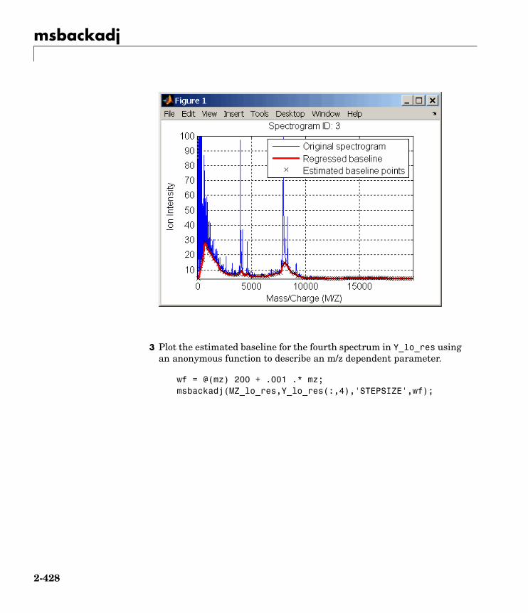
msbackadj
3 Plot the estimated baseline for the fourth spectrum in Y_lo_res usingan anonymous function to describe an m/z dependent parameter.
wf = @(mz) 200 + .001 .* mz;msbackadj(MZ_lo_res,Y_lo_res(:,4),'STEPSIZE',wf);
2-428

msbackadj
See Also Bioinformatics Toolbox functions msalign, mslowess, msheatmap,msnorm, mspeaks, msresample, mssgolay, msviewer
2-429
msdotplot
Purpose Plot set of peak lists from LC/MS or GC/MS data set
Syntax msdotplot(Peaks, Times)msdotplot(FigHandle, Peaks, Times)msdotplot(..., 'Quantile', QuantileValue)PlotHandle = msdotplot(...)
ArgumentsPeaks Cell array of peak lists, where each element is a
two-column matrix with m/z values in the firstcolumn and ion intensity values in the secondcolumn. Each element corresponds to a spectrumor retention time.
Tip You can use the mzxml2peaks function tocreate the Peaks cell array.
Times Vector of retention times associated with an LC/MSor GC/MS data set. The number of elements inTimes equals the number of elements in the cellarray Peaks.
Tip You can use the mzxml2peaks function tocreate the Times vector.
FigHandle Handle to an open Figure window such as onecreated by the msheatmap function.
QuantileValue Value that specifies a percentage. When peaks areranked by intensity, only those that rank abovethis percentage are plotted. Choices are any value≥ 0 and ≤ 1. Default is 0. For example, settingQuantileValue = 0 plots all peaks, and settingQuantileValue = 0.8 plots only the 20% mostintense peaks.
2-430
msdotplot
ReturnValues
PlotHandle Handle to the line series object (figure plot).
Description msdotplot(Peaks, Times) plots a set of peak lists from aliquid chromatography/mass spectrometry (LC/MS) or gaschromatography/mass spectrometry (GC/MS) data set represented byPeaks, a cell array of peak lists, where each element is a two-columnmatrix with m/z values in the first column and ion intensity values inthe second column, and Times, a vector of retention times associatedwith the spectra. Peaks and Times have the same number of elements.The data is plotted into any existing figure generated by the msheatmapfunction; otherwise, the data is plotted into a new Figure window.
msdotplot(FigHandle, Peaks, Times) plots the set of peak listsinto the axes contained in an open Figure window with the handleFigHandle.
Tip This syntax is useful to overlay a dot plot on top of a heat map ofmass spectrometry data created with the msheatmap function.
msdotplot(..., 'Quantile', QuantileValue) plots only the mostintense peaks, specifically those in the percentage above the specifiedQuantileValue. Choices are any value ≥ 0 and ≤ 1. Default is 0.For example, setting QuantileValue = 0 plots all peaks, and settingQuantileValue = 0.8 plots only the 20% most intense peaks.
PlotHandle = msdotplot(...) returns a handle to the line seriesobject (figure plot). You can use this handle as input to the get functionto display a list of the plot’s properties. You can use this handle as inputto the set function to change the plot’s properties, including showingand hiding points.
Examples 1 Load a MAT file, included with Bioinformatics Toolbox, whichcontains LC/MS data variables, including peaks and ret_time.peaks is a cell array of peak lists, where each element is a two-column
2-431

msdotplot
matrix of m/z values and ion intensity values, and each elementcorresponds to a spectrum or retention time. ret_time is a columnvector of retention times associated with the LC/MS data set.
load lcmsdata
2 Create a dot plot with only the 5% most intense peaks.
msdotplot(peaks,ret_time,'Quantile',0.95)
2-432
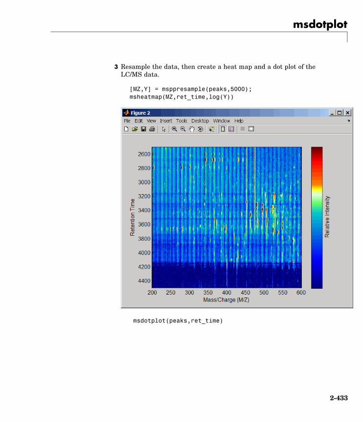
msdotplot
3 Resample the data, then create a heat map and a dot plot of theLC/MS data.
[MZ,Y] = msppresample(peaks,5000);msheatmap(MZ,ret_time,log(Y))
msdotplot(peaks,ret_time)
2-433

msdotplot
4 Zoom in on the heat map to see the detail.
axis([470 520 3200 3600])
2-434
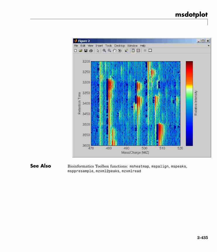
msdotplot
See Also Bioinformatics Toolbox functions: msheatmap, mspalign, mspeaks,msppresample, mzxml2peaks, mzxmlread
2-435
msheatmap
Purpose Create pseudocolor image of set of mass spectra
Syntax msheatmap(MZ, Intensities)msheatmap(MZ, Times, Intensities)msheatmap(..., 'Midpoint', MidpointValue, ...)msheatmap(..., 'Range', RangeValue, ...)msheatmap(..., 'Markers', MarkersValue, ...)msheatmap(..., 'SpecIdx', SpecIdxValue, ...)msheatmap(..., 'Group', GroupValue, ...)msheatmap(..., 'Resolution', ResolutionValue, ...)
ArgumentsMZ Column vector of common mass/charge (m/z)
values for a set of spectra. The number of elementsin the vector equals the number of rows in thematrix Intensities.
Note You can use the msppresample function tocreate the MZ vector.
Times Column vector of retention times associatedwith a liquid chromatography/mass spectrometry(LC/MS) or gas chromatography/mass spectrometry(GC/MS) data set. The number of elements in thevector equals the number of columns in the matrixIntensities. The retention times are used tolabel the y-axis of the heat map.
Tip You can use the mzxml2peaks function tocreate the Times vector.
2-436

msheatmap
Intensities Matrix of intensity values for a set of massspectra that share the same m/z range. Each rowcorresponds to an m/z value, and each columncorresponds to a spectrum or retention time. Thenumber of rows equals the number of elementsin vector MZ. The number of columns equals thenumber of elements in vector Times.
Note You can use the msppresample function tocreate the Intensities matrix.
2-437

msheatmap
MidpointValue Value specifying a quantile of the ion intensityvalues to fall below the midpoint of the colormap, meaning they do not represent peaks.msheatmap uses a custom color map where coolcolors represent nonpeak regions, white representsthe midpoint, and warm colors represent peaks.Choices are any value ≥ 0 and ≤ 1. Default is:
• 0.99 — For LC/MS or GC/MS data or wheninput T is provided. This means that 1% of thepixels are warm colors and represent peaks.
• 0.95 — For non-LC/MS or non-GC/MS data orwhen input T is not provided. This means that5% of the pixels are warm colors and representpeaks.
Tip You can also change the midpoint interactivelyafter creating the heat map by right-clicking thecolor bar, selecting Interactive Colormap Shift,and then click-dragging the cursor vertically on thecolor bar. This technique is useful when comparingmultiple heat maps.
RangeValue 1-by-2 vector specifying the m/z range for thex-axis of the heat map. RangeValue must be within[min(MZ) max(MZ)]. Default is the full range[min(MZ) max(MZ)].
MarkersValue Vector of m/z values to mark on the top horizontalaxis of the heat map. Default is [].
2-438
msheatmap
SpecIdxValue Either of the following:• Vector of values with the same number of
elements as columns (spectra) in the matrixIntensities.
• Cell array of strings with the same number ofelements as columns (spectra) in the matrixIntensities.
Each value or string specifies a label for thecorresponding spectrum. These values or stringsare used to label the y-axis of the heat map.
Note If input Times is provided, it is assumedthat Intensities contains LC/MS or GC/MS data,and SpecIdxValue is ignored.
2-439

msheatmap
GroupValue Either of the following:• Vector of values with the same number of
elements as rows in the matrix Intensities
• Cell array of strings with the same numberof elements as rows (spectra) in the matrixIntensities
Each value or string specifies a group to which thecorresponding spectrum belongs. The spectra aresorted and combined into groups along the y-axisin the heat map.
Note If input Times is provided, it is assumedthat Intensities contains LC/MS or GC/MS data,and GroupValue is ignored.
ResolutionValue Value specifying the horizontal resolution of theheat map image. Increase this value to enhancedetails. Decrease this value to reduce memoryusage. Default is:• 0.5 — When MZ contains > 2,500 elements.
• 0.05 — When MZ contains <= 2,500 elements.
Description msheatmap(MZ, Intensities) displays a pseudocolor heat map imageof the intensities for the spectra in matrix Intensities.
msheatmap(MZ, Times, Intensities) displays a pseudocolor heatmap image of the intensities for the spectra in matrix Intensities,using the retention times in vector Times to label the y-axis.
msheatmap(..., 'PropertyName', PropertyValue, ...) callsmsheatmap with optional properties that use property name/propertyvalue pairs. You can specify one or more properties in any order. EachPropertyName must be enclosed in single quotation marks and is caseinsensitive. These property name/property value pairs are as follows:
2-440
msheatmap
msheatmap(..., 'Midpoint', MidpointValue, ...) specifies aquantile of the ion intensity values to fall below the midpoint of thecolor map, meaning they do not represent peaks. msheatmap uses acustom color map where cool colors represent nonpeak regions, whiterepresents the midpoint, and warm colors represent peaks. Choices areany value between 0 and 1. Default is:
• 0.99 — For LC/MS or GC/MS data or when input T is provided. Thismeans that 1% of the pixels are warm colors and represent peaks.
• 0.95 — For non-LC/MS or non-GC/MS data or when input T is notprovided. This means that 5% of the pixels are warm colors andrepresent peaks.
Tip You can also change the midpoint interactively after creatingthe heat map by right-clicking the color bar, selecting InteractiveColormap Shift, then click-dragging the cursor vertically on the colorbar. This technique is useful when comparing multiple heat maps.
msheatmap(..., 'Range', RangeValue, ...) specifies the m/z rangefor the x-axis of the heat map. RangeValue is a 1-by-2 vector that mustbe within [min(MZ) max(MZ)]. Default is the full range [min(MZ)max(MZ)].
msheatmap(..., 'Markers', MarkersValue, ...) places markersalong the top horizontal axis of the heat map for the m/z values specifiedin the vector MarkersValue. Default is [].
msheatmap(..., 'SpecIdx', SpecIdxValue, ...) labels thespectra along the y-axis in the heat map. The labels are specified bySpecIdxValue, a vector of values or cell array of strings. The numberof values or strings is the same as the number of columns (spectra) inthe matrix Intensities. Each value or string specifies a label for thecorresponding spectrum.
msheatmap(..., 'Group', GroupValue, ...) sorts and combinesspectra into groups along the y-axis in the heat map. The groups are
2-441
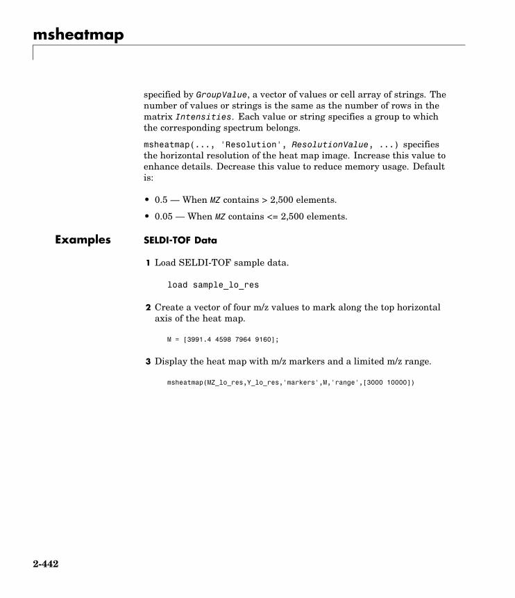
msheatmap
specified by GroupValue, a vector of values or cell array of strings. Thenumber of values or strings is the same as the number of rows in thematrix Intensities. Each value or string specifies a group to whichthe corresponding spectrum belongs.
msheatmap(..., 'Resolution', ResolutionValue, ...) specifiesthe horizontal resolution of the heat map image. Increase this value toenhance details. Decrease this value to reduce memory usage. Defaultis:
• 0.5 — When MZ contains > 2,500 elements.
• 0.05 — When MZ contains <= 2,500 elements.
Examples SELDI-TOF Data
1 Load SELDI-TOF sample data.
load sample_lo_res
2 Create a vector of four m/z values to mark along the top horizontalaxis of the heat map.
M = [3991.4 4598 7964 9160];
3 Display the heat map with m/z markers and a limited m/z range.
msheatmap(MZ_lo_res,Y_lo_res,'markers',M,'range',[3000 10000])
2-442
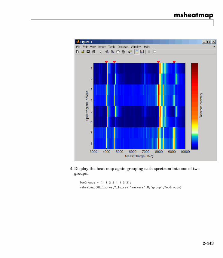
msheatmap
4 Display the heat map again grouping each spectrum into one of twogroups.
TwoGroups = [1 1 2 2 1 1 2 2];
msheatmap(MZ_lo_res,Y_lo_res,'markers',M,'group',TwoGroups)
2-443
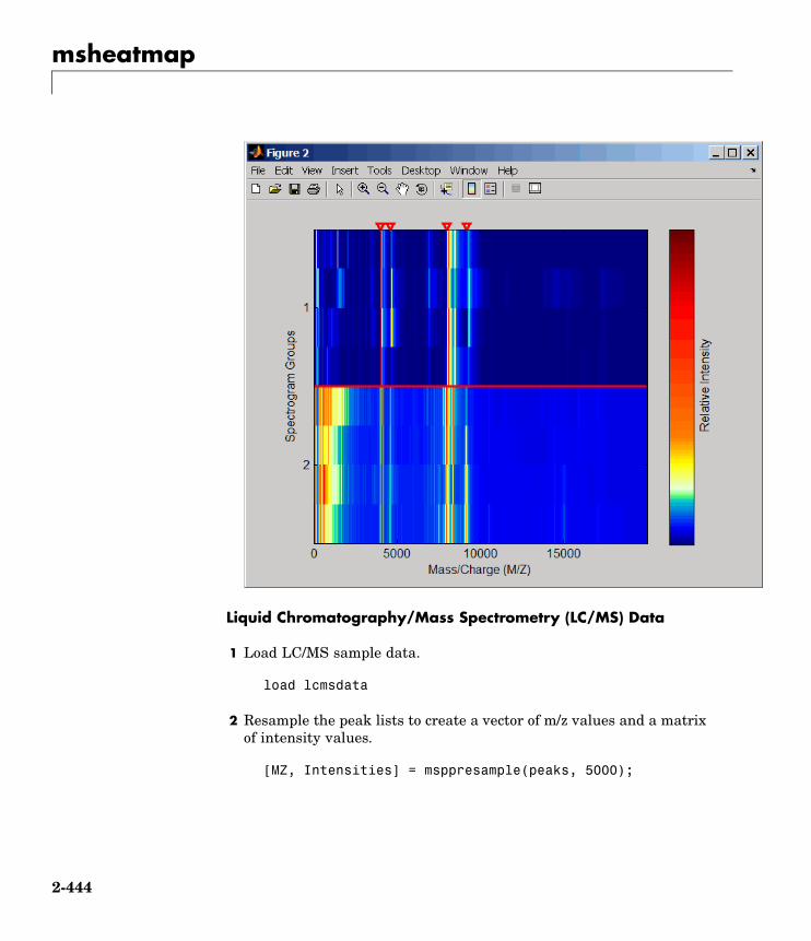
msheatmap
Liquid Chromatography/Mass Spectrometry (LC/MS) Data
1 Load LC/MS sample data.
load lcmsdata
2 Resample the peak lists to create a vector of m/z values and a matrixof intensity values.
[MZ, Intensities] = msppresample(peaks, 5000);
2-444

msheatmap
3 Display the heat map showing mass spectra at different retentiontimes.
msheatmap(MZ, ret_time, log(Intensities))
See Also Bioinformatics Toolbox functions: msalign, msbackadj, msdotplot,mslowess, msnorm, mspalign, msresample, mssgolay, msviewer
2-445

mslowess
Purpose Smooth mass spectrum using nonparametric method
Syntax Yout = mslowess(MZ, Y, 'PropertyName', PropertyValue...)mslowess(..., 'Order', OrderValue)mslowess(..., 'Span', SpanValue)mslowess(..., 'Kernel', KernelValue)mslowess(..., 'RobustIterations', RobustIterationsValue)mslowess(..., 'ShowPlot', ShowPlotValue)
ArgumentsMZ Mass/charge vector with the range of ions in the
spectra.
Y Ion intensity vector with the same length as themass/charge vector (MZ). Y can also be a matrix withseveral spectra that share the same mass/charge (MZ)range.
Description Yout = mslowess(MZ, Y, 'PropertyName', PropertyValue...)smoothes a mass spectrum (Y) using a locally weighted linear regression(lowess) method with a default span of 10 samples.
Note 1) mslowess assumes that a mass/charge vector (MZ) might notbe uniformly spaced. Therefore, the sliding window for smoothing iscentered using the closest samples in terms of the MZ value and notin terms of the MZ indices.
2) When the vector MZ does not have repeated values or NaNs, thealgorithm is approximately twice as fast.
mslowess(..., 'Order', OrderValue) specifies the order(OrderValue) of the Lowess smoother. Enter 1 (linear polynomial fit orLowess), 2 (quadratic polynomial fit or Loess), or 0 (equivalent to aweighted local mean estimator and presumably faster because only a
2-446
mslowess
mean computation is performed instead of a least squares regression).The default value is 1.
Note Curve Fitting Toolbox also refers to Lowess smoothing of order 2as Loess smoothing.
mslowess(..., 'Span', SpanValue) specifies the window size for thesmoothing kernel. If SpanValue is greater than 1, the window is equalto SpanValue number of samples independent of the mass/charge vector(MZ). The default value is 10 samples. Higher values will smooth thesignal more at the expense of computation time. If SpanValue is lessthan 1, the window size is taken to be a fraction of the number of pointsin the data. For example, when SpanValue is 0.005, the window size isequal to 0.50% of the number of points in MZ.
mslowess(..., 'Kernel', KernelValue) selects the function(KernelValue) for weighting the observed ion intensities. Samples closeto the MZ location being smoothed have the most weight in determiningthe estimate. Enter
'tricubic' (default) (1 - (dist/dmax).^3).^3'gaussian' exp(-(2*dist/dmax).^2)'linear' 1-dist/dmax
mslowess(..., 'RobustIterations', RobustIterationsValue)specifies the number of iterations (RobustValue) for a robust fit. IfRobustIterationsValue is 0 (default), no robust fit is performed. Forrobust smoothing, small residual values at every span are outweighed toimprove the new estimate. 1 or 2 robust iterations are usually adequatewhile, larger values might be computationally expensive.
2-447

mslowess
Note For a uniformly spaced MZ vector, a nonrobust smoothing withOrder equal to 0 is equivalent to filtering the signal with the kernelvector.
mslowess(..., 'ShowPlot', ShowPlotValue)plots the smoothedspectrum over the original spectrum. When mslowess is called withoutoutput arguments, the spectra are plotted unless ShowPlotValue isfalse. When ShowPlotValue is true, only the first spectrum in Y isplotted. ShowPlotValue can also contain an index to one of the spectrain Y.
Example 1 Load sample data.
load sample_lo_res
2 Smooth spectrum and draw figure with unsmoothed and smoothedspectra.
YS = mslowess(MZ_lo_res,Y_lo_res(:,1),'Showplot',true);
2-448

mslowess
2-449

mslowess
See Also Bioinformatics Toolbox functions msalign, msbackadj, msheatmap,msheatmap,msnorm, mspeaks, msresample, mssgolay, msviewer
2-450

msnorm
Purpose Normalize set of mass spectra
Syntax Yout = msnorm(MZ, Y)[Yout, NormParameters] = msnorm(...)msnorm(MZ, NewY, NormParameters)msnorm(..., 'PropertyName', PropertyValue,...)msnorm(..., 'Quantile', QuantileValue)msnorm(..., 'Limits', LimitsValue)msnorm(..., 'Consensus', ConsensusValue)msnorm(..., 'Method', MethodValue)msnorm(..., 'Max', MaxValue)
ArgumentsMZ Mass/charge vector with the range of ions in the
spectra.
Y Ion intensity vector with the same length as themass/charge vector (MZ). Y can also be a matrix withseveral spectra that share the same mass/charge (MZ)range.
Description Yout = msnorm(MZ, Y) normalizes a group of mass spectra bystandardizing the area under the curve (AUC) to the group median.
[Yout, NormParameters] = msnorm(...) returns a structure withthe parameters to normalize another group of spectra.
msnorm(MZ, NewY, NormParameters) uses the parameter informationfrom a previous normalization (NormParameters) to normalize a newset of spectra (NewY) with the MZ positions and output scale from theprevious normalization. NormParameters is a structure created bymsnorm. If a consensus proportion (ConsensusValue) was given inthe previous normalization, no new MZ positions are selected, andnormalization is performed using the same MZ positions.
msnorm(..., 'PropertyName', PropertyValue,...) defines optionalproperties using property name/value pairs.
2-451
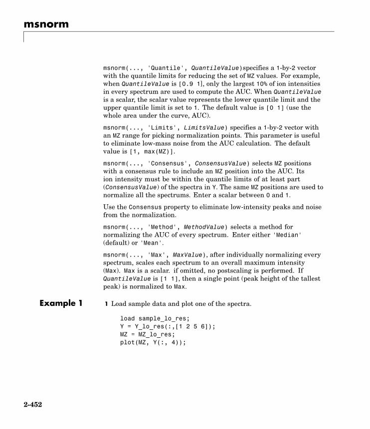
msnorm
msnorm(..., 'Quantile', QuantileValue)specifies a 1-by-2 vectorwith the quantile limits for reducing the set of MZ values. For example,when QuantileValue is [0.9 1], only the largest 10% of ion intensitiesin every spectrum are used to compute the AUC. When QuantileValueis a scalar, the scalar value represents the lower quantile limit and theupper quantile limit is set to 1. The default value is [0 1] (use thewhole area under the curve, AUC).
msnorm(..., 'Limits', LimitsValue) specifies a 1-by-2 vector withan MZ range for picking normalization points. This parameter is usefulto eliminate low-mass noise from the AUC calculation. The defaultvalue is [1, max(MZ)].
msnorm(..., 'Consensus', ConsensusValue) selects MZ positionswith a consensus rule to include an MZ position into the AUC. Itsion intensity must be within the quantile limits of at least part(ConsensusValue) of the spectra in Y. The same MZ positions are used tonormalize all the spectrums. Enter a scalar between 0 and 1.
Use the Consensus property to eliminate low-intensity peaks and noisefrom the normalization.
msnorm(..., 'Method', MethodValue) selects a method fornormalizing the AUC of every spectrum. Enter either 'Median'(default) or 'Mean'.
msnorm(..., 'Max', MaxValue), after individually normalizing everyspectrum, scales each spectrum to an overall maximum intensity(Max). Max is a scalar. if omitted, no postscaling is performed. IfQuantileValue is [1 1], then a single point (peak height of the tallestpeak) is normalized to Max.
Example 1 1 Load sample data and plot one of the spectra.
load sample_lo_res;Y = Y_lo_res(:,[1 2 5 6]);MZ = MZ_lo_res;plot(MZ, Y(:, 4));
2-452
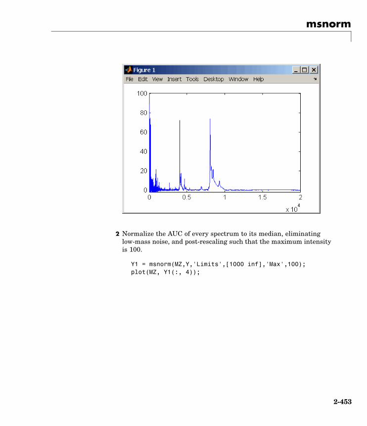
msnorm
2 Normalize the AUC of every spectrum to its median, eliminatinglow-mass noise, and post-rescaling such that the maximum intensityis 100.
Y1 = msnorm(MZ,Y,'Limits',[1000 inf],'Max',100);plot(MZ, Y1(:, 4));
2-453

msnorm
3 Normalize the ion intensity of every spectrum to the maximumintensity of the single highest peak from any of the spectra in therange above 100 m/z.
Y2 = msnorm(MZ,Y,'QUANTILE', [1 1],'LIMITS',[1000 inf]);
Example 2 1 Select MZ regions where the intensities are within the third quartilein at least 90% of the spectrograms.
[Y3,S] = msnorm(MZ,Y,'Quantile',[0.5 0.75],'Consensus',0.9);
2 Use the same MZ regions to normalize another set of spectrograms.
Y4 = msnorm(MZ,Y,S);
See Also Bioinformatics Toolbox functions msalign, msbackadj, msheatmap,mslowess, msresample, mssgolay, msviewer
2-454
mspalign
Purpose Align mass spectra from multiple peak lists from LC/MS or GC/MSdata set
Syntax [CMZ, AlignedPeaks] = mspalign(Peaks)[CMZ, AlignedPeaks] = mspalign(Peaks, ...'Quantile',QuantileValue, ...)[CMZ, AlignedPeaks] = mspalign(Peaks,...'EstimationMethod',
EstimationMethodValue, ...)[CMZ, AlignedPeaks] = mspalign(Peaks,...'CorrectionMethod',
CorrectionMethodValue, ...)
Arguments Peaks Cell array of peak lists from a liquidchromatography/mass spectrometry(LC/MS) or gas chromatography/massspectrometry (GC/MS) data set. Eachelement in the cell array is a two-columnmatrix with m/z values in the first columnand ion intensity values in the secondcolumn. Each element corresponds to aspectrum or retention time.
Note You can use the mzxml2peaksfunction or the mspeaks function to createthe Peaks cell array.
QuantileValue Value that determines which peaks areselected by the estimation method to createCMZ, the vector of common m/z values.Choices are any value ≥ 0 and ≤ 1. Defaultis 0.95.
2-455

mspalign
EstimationMethodValueString specifying the method to estimateCMZ, the vector of common mass/charge (m/z)values. Choices are:
• histogram — Default method. Peaklocations are clustered using a kerneldensity estimation approach. The peakion intensity is used as a weighting factor.The center of all the clusters conform tothe CMZ vector.
• regression — Takes a sample of thedistances between observed significantpeaks and regresses the inter-peakdistance to create the CMZ vector withsimilar inter-element distances.
CorrectionMethodValueString specifying the method to align eachpeak list to the CMZ vector. Choices are:
• nearest-neighbor — Default method.For each common peak in the CMZ vector,its counterpart in each peak list is thepeak that is closest to the common peak’sm/z value.
• shortest-path — For each common peakin the CMZ vector, its counterpart in eachpeak list is selected using the shortestpath algorithm.
ReturnValues
CMZ Vector of common mass/charge (m/z) valuesestimated by the mspalign function.
AlignedPeaks Cell array of peak lists, with the same formas Peaks, but with corrected m/z values inthe first column of each matrix.
2-456
mspalign
Description [CMZ, AlignedPeaks] = mspalign(Peaks) aligns mass spectra frommultiple peak lists (centroided data), by first estimating CMZ, a vector ofcommon mass/charge (m/z) values estimated by considering the peaksin all spectra in Peaks, a cell array of peak lists, where each elementcorresponds to a spectrum or retention time. It then aligns the peaksin each spectrum to the values in CMZ, creating AlignedPeaks, a cellarray of aligned peak lists.
[CMZ, AlignedPeaks] = mspalign(Peaks, ...'PropertyName',PropertyValue, ...) calls mspalign with optional properties thatuse property name/property value pairs. You can specify one or moreproperties in any order. Each PropertyName must be enclosed in singlequotation marks and is case insensitive. These property name/propertyvalue pairs are as follows:
[CMZ, AlignedPeaks] = mspalign(Peaks, ...'Quantile',QuantileValue, ...) determines which peaks are selected by theestimation method to create CMZ, the vector of common m/z values.Choices are a scalar between 0 and 1. Default is 0.95.
[CMZ, AlignedPeaks] = mspalign(Peaks,...'EstimationMethod', EstimationMethodValue,...) specifies the method used to estimate CMZ, the vector of commonmass/charge (m/z) values. Choices are:
• histogram — Default method. Peak locations are clustered using akernel density estimation approach. The peak ion intensity is usedas a weighting factor. The center of all the clusters conform to theCMZ vector.
• regression — Takes a sample of the distances between observedsignificant peaks and regresses the inter-peak distance to create theCMZ vector with similar inter-element distances.
[CMZ, AlignedPeaks] = mspalign(Peaks,...'CorrectionMethod', CorrectionMethodValue,...) specifies the method used to align each peak list to the CMZ vector.Choices are:
2-457
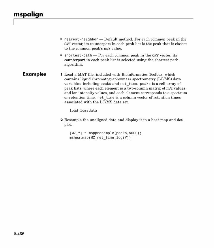
mspalign
• nearest-neighbor — Default method. For each common peak in theCMZ vector, its counterpart in each peak list is the peak that is closestto the common peak’s m/z value.
• shortest-path — For each common peak in the CMZ vector, itscounterpart in each peak list is selected using the shortest pathalgorithm.
Examples 1 Load a MAT file, included with Bioinformatics Toolbox, whichcontains liquid chromatography/mass spectrometry (LC/MS) datavariables, including peaks and ret_time. peaks is a cell array ofpeak lists, where each element is a two-column matrix of m/z valuesand ion intensity values, and each element corresponds to a spectrumor retention time. ret_time is a column vector of retention timesassociated with the LC/MS data set.
load lcmsdata
2 Resample the unaligned data and display it in a heat map and dotplot.
[MZ,Y] = msppresample(peaks,5000);msheatmap(MZ,ret_time,log(Y))
2-458

mspalign
msdotplot(peaks,ret_time)
2-459
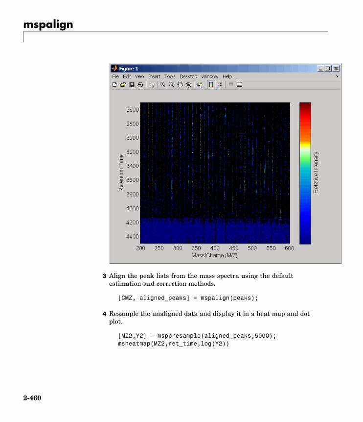
mspalign
3 Align the peak lists from the mass spectra using the defaultestimation and correction methods.
[CMZ, aligned_peaks] = mspalign(peaks);
4 Resample the unaligned data and display it in a heat map and dotplot.
[MZ2,Y2] = msppresample(aligned_peaks,5000);msheatmap(MZ2,ret_time,log(Y2))
2-460
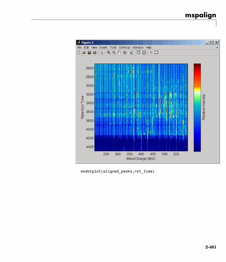
mspalign
msdotplot(aligned_peaks,ret_time)
2-461

mspalign
5 Link the axes of the two heat plots and zoom in to observe the detail.
linkaxes(findobj(0,'Tag','MSHeatMap'))axis([570 590 3750 3900])
2-462

mspalign
2-463

mspalign
References [1] Jeffries, N. (2005) Algorithms for alignment of mass spectrometryproteomic data. Bioinfomatics 21:14, 3066–3073.
[2] Purvine, S., Kolker, N., and Kolker, E. (2004) Spectral QualityAssessment for High-Throughput Tandem Mass SpectrometryProteomics. OMICS: A Journal of Integrative Biology 8:3, 255–265.
See Also Bioinformatics Toolbox functions: msalign, msdotplot, msheatmap,mspeaks , msppresample, mzxml2peaks
2-464
mspeaks
Purpose Convert raw mass spectrometry data to peak list (centroided data)
Syntax Peaks = mspeaks(MZ, Intensities)Peaks = mspeaks(MZ, Intensities, ...'Base', BaseValue, ...)Peaks = mspeaks(MZ, Intensities, ...'Levels', LevelsValue,
...)Peaks = mspeaks(MZ, Intensities, ...'NoiseEstimator',
NoiseEstimatorValue, ...)Peaks = mspeaks(MZ, Intensities, ...'Multiplier',
MultiplierValue, ...)Peaks = mspeaks(MZ, Intensities, ...'Denoising',
DenoisingValue, ...)Peaks = mspeaks(MZ, Intensities, ...'PeakLocation',
PeakLocationValue, ...)Peaks = mspeaks(MZ, Intensities, ...'FWHH_Filter',
FWHH_FilterValue, ...)Peaks = mspeaks(MZ, Intensities,...'OverSegmentation_Filter',
OverSegmentation_FilterValue, ...)Peaks = mspeaks(MZ, Intensities, ...'Height_Filter',
Height_FilterValue, ...)Peaks = mspeaks(MZ, Intensities, ...'ShowPlot',
ShowPlotValue, ...)
2-465

mspeaks
ArgumentsMZ Vector of mass/charge (m/z) values
for a set of spectra. The numberof elements in the vector equals nor the number of rows in matrixIntensities.
Intensities Matrix of intensity values for a setof mass spectra that share the samemass/charge (m/z) range. Eachrow corresponds to an m/z value,and each column corresponds to aspectrum or retention time. Thenumber of rows equals n or thenumber of elements in vector MZ.
BaseValue An integer between 2 and 20 thatspecifies the wavelet base. Defaultis 4.
LevelsValue An integer between 1 and 12 thatspecifies the number of levels forthe wavelet decomposition. Defaultis 10.
2-466
mspeaks
NoiseEstimatorValue String or scalar that specifies themethod to estimate the threshold, T,to filter out noisy components in thefirst high-band decomposition (y_h).Choices are:
• mad — Default. Median absolutedeviation, which calculates T =sqrt(2*log(n))*mad(y_h) /0.6745, where n = the number ofrows in the Intensities matrix.
• std — Standard deviation, whichcalculates T = std(y_h).
• A positive real value.
MultiplierValue A positive real value that specifiesthe threshold multiplier constant.Default is 1.0.
DenoisingValue Controls the use of waveletdenoising to smooth the signal.Choices are true (default) or false.
Note If your data has previouslybeen smoothed, for example, withthe mslowess or mssgolay function,it is not necessary to use waveletdenoising. Set this property tofalse.
2-467

mspeaks
PeakLocationValue Value that specifies the proportionof the peak height that selects thepoints used to compute the centroidmass of the respective peak. Thevalue must be ≥ 0 and ≤ 1. Defaultis 1.0.
FWHH_FilterValue Positive real value that specifies theminimum full width at half height(FWHH), in m/z units, for reportedpeaks. Peaks with FWHH belowthis value are not included in theoutput list Peaks. Default is 0.
OverSegmentation_FilterValuePositive real value that specifiesthe minimum distance, in m/zunits, between neighboring peaks.When the signal is not smoothedappropriately, multiple maximacan appear to represent the samepeak. By increasing this filter value,oversegmented peaks are joined intoa single peak. Default is 0.
2-468

mspeaks
Height_FilterValue Positive real value that specifies theminimum height for reported peaks.Default is 0.
ShowPlotValue Controls the display of a plot ofthe original and the smoothedsignal, with the peaks included inthe output matrix Peaks marked.Choices are true, false, or I,an integer specifying the index ofa spectrum in Intensities. Ifset to true, the first spectrum inIntensities is plotted. Default is:
• false — When return values arespecified.
• true — When return values arenot specified.
ReturnValues
Peaks Two-column matrix where eachrow corresponds to a peak. Thefirst column contains mass/charge(m/z) values, and the second columncontains ion intensity values.
Description Peaks = mspeaks(MZ, Intensities) finds relevant peaks in raw massspectrometry data, and creates Peaks, a two-column matrix, containingthe m/z value and ion intensity for each peak.
mspeaks finds peaks by first smoothing the signal using undecimatedwavelet transform with Daubechies coefficients, then assigning peaklocations, and lastly, eliminating peaks that do not satisfy specifiedcriteria.
Peaks = mspeaks(MZ, Intensities, ...'PropertyName',PropertyValue, ...) calls mspeaks with optional properties that
2-469
mspeaks
use property name/property value pairs. You can specify one or moreproperties in any order. Each PropertyName must be enclosed in singlequotation marks and is case insensitive. These property name/propertyvalue pairs are as follows:
Peaks = mspeaks(MZ, Intensities, ...'Base', BaseValue, ...)specifies the wavelet base. BaseValue must be an integer between 2and 20. Default is 4.
Peaks = mspeaks(MZ, Intensities, ...'Levels', LevelsValue,...) specifies the number of levels for the wavelet decomposition.LevelsValue must be an integer between 1 and 12. Default is 10.
Peaks = mspeaks(MZ, Intensities, ...'NoiseEstimator',NoiseEstimatorValue, ...) specifies the method to estimate thethreshold, T, to filter out noisy components in the first high-banddecomposition (y_h). Choices are:
• mad — Default. Median absolute deviation, which calculates T =sqrt(2*log(n))*mad(y_h) / 0.6745, where n = the number of rowsin the Intensities matrix.
• std — Standard deviation, which calculates T = std(y_h).
• A positive real value.
Peaks = mspeaks(MZ, Intensities, ...'Multiplier',MultiplierValue, ...) specifies the threshold multiplier constant.MultiplierValue must be a positive real value. Default is 1.0.
Peaks = mspeaks(MZ, Intensities, ...'Denoising',DenoisingValue, ...) controls the use of wavelet denoising to smooththe signal. Choices are true (default) or false.
2-470

mspeaks
Note If your data has previously been smoothed, for example, withthe mslowess or mssgolay function, it is not necessary to use waveletdenoising. Set this property to false.
Peaks = mspeaks(MZ, Intensities, ...'PeakLocation',PeakLocationValue, ...) specifies the proportion of the peak heightthat selects the points used to compute the centroid mass of therespective peak. PeakLocationValue must be a value ≥ 0 and ≤ 1.Default is 1.0.
Note When PeakLocationValue = 1.0, the peak location is exactly atthe maximum of the peak, while when PeakLocationValue = 0, thepeak location is computed with all the points from the closest minimumto the left of the peak to the closest minimum to the right of the peak.
Peaks = mspeaks(MZ, Intensities, ...'FWHH_Filter',FWHH_FilterValue, ...) specifies the minimum full width athalf height (FWHH), in m/z units, for reported peaks. Peaks withFWHH below this value are not included in the output list Peaks.FWHH_FilterValue must be a positive real value. Default is 0.
Peaks = mspeaks(MZ, Intensities,...'OverSegmentation_Filter', OverSegmentation_FilterValue,...) specifies the minimum distance, in m/z units, betweenneighboring peaks. When the signal is not smoothed appropriately,multiple maxima can appear to represent the same peak. By increasingthis filter value, oversegmented peaks are joined into a single peak.OverSegmentation_FilterValue must be a positive real value.Default is 0.
Peaks = mspeaks(MZ, Intensities, ...'Height_Filter',Height_FilterValue, ...) specifies the minimum height for reported
2-471
mspeaks
peaks. Peaks with heights below this value are not included in theoutput list Peaks. Height_FilterValue must be a positive real value.Default is 0.
Peaks = mspeaks(MZ, Intensities, ...'ShowPlot',ShowPlotValue, ...) controls the display of a plot of the original andthe smoothed signal, with the peaks included in the output matrixPeaks marked. Choices are true, false, or I, an integer specifying theindex of a spectrum in Intensities. If set to true, the first spectrumin Intensities is plotted. Default is:
• false — When return values are specified.
• true — When return values are not specified.
Examples 1 Load a MAT file, included with Bioinformatics Toolbox, whichcontains mass spectrometry data variables, including MZ_lo_res, avector of m/z values for a set of spectra, and Y_lo_res, a matrix ofintensity values for a set of mass spectra that share the same m/zrange.
load sample_lo_res
2 Adjust the baseline of the eight spectra stored in Y_lo_res.
YB = msbackadj(MZ_lo_res,Y_lo_res);
3 Convert the raw mass spectrometry data to a peak list by finding therelevant peaks in each spectrum.
P = mspeaks(MZ_lo_res,YB);
4 Plot the third spectrum in YB, the matrix of baseline-correctedintensity values, with the detected peaks marked.
P = mspeaks(MZ_lo_res,YB,'SHOWPLOT',3);
2-472

mspeaks
5 Smooth the signal using the mslowess function. Then convert thesmoothed data to a peak list by finding relevant peaks and plot thethird spectrum.
YS = mslowess(MZ_lo_res,YB,'SHOWPLOT',3);
2-473

mspeaks
P = mspeaks(MZ_lo_res,YS,'DENOISING',false,'SHOWPLOT',3);
2-474

mspeaks
6 Use the cellfun function to remove all peaks with m/z values lessthan 2000 from the eight peaks lists in output P. Then plot the peaksof the third spectrum (in red) over its smoothed signal (in blue).
Q = cellfun(@(p) p(p(:,1)>2000,:),P,'UniformOutput',false);figureplot(MZ_lo_res,YS(:,3),'b',Q{3}(:,1),Q{3}(:,2),'rx')xlabel('Mass/Charge (M/Z)')ylabel('Relative Intensity')axis([0 20000 -5 95])
2-475
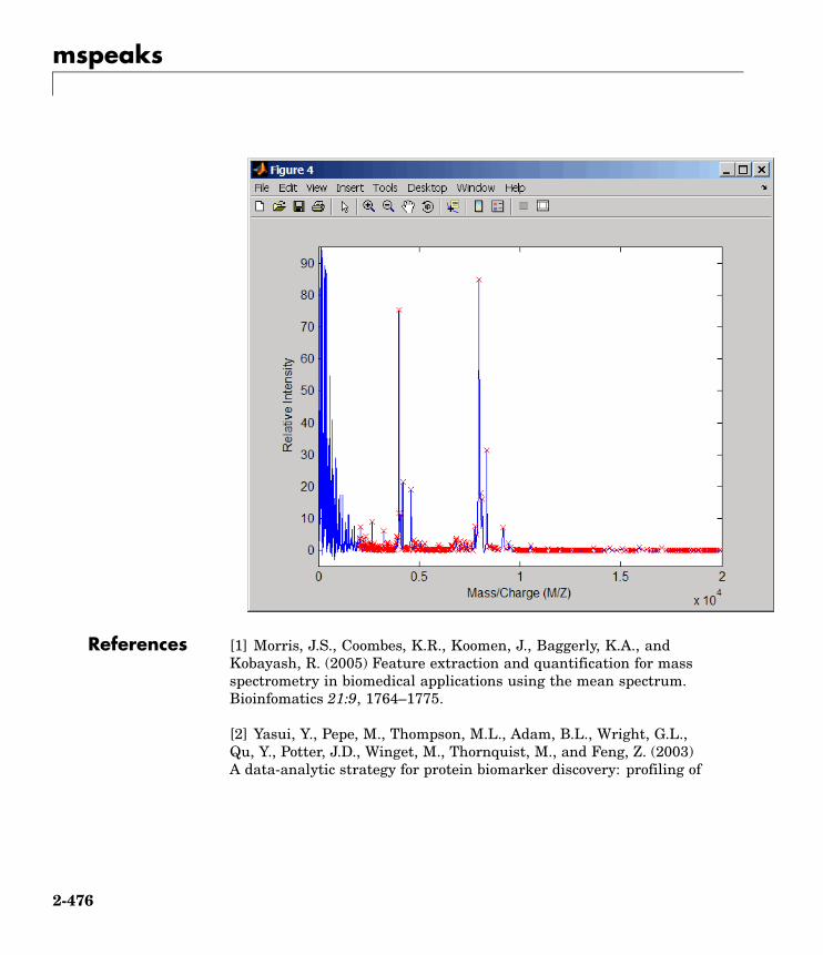
mspeaks
References [1] Morris, J.S., Coombes, K.R., Koomen, J., Baggerly, K.A., andKobayash, R. (2005) Feature extraction and quantification for massspectrometry in biomedical applications using the mean spectrum.Bioinfomatics 21:9, 1764–1775.
[2] Yasui, Y., Pepe, M., Thompson, M.L., Adam, B.L., Wright, G.L.,Qu, Y., Potter, J.D., Winget, M., Thornquist, M., and Feng, Z. (2003)A data-analytic strategy for protein biomarker discovery: profiling of
2-476

mspeaks
high-dimensional proteomic data for cancer detection. Biostatistics4:3, 449–463.
[3] Donoho, D.L., and Johnstone, I.M. (1995) Adapting to unknownsmoothness via wavelet shrinkage. J. Am. Statist. Asso. 90, 1200–1224.
[4] Strang, G., and Nguyen, T. (1996) Wavelets and Filter Banks(Wellesley: Cambridge Press).
[5] Coombes, K.R., Tsavachidis, S., Morris, J.S., Baggerly, K.A.,Hung, M.C., and Kuerer, H.M. (2005) Improved peak detectionand quantification of mass spectrometry data acquired fromsurface-enhanced laser desorption and ionization by denoising spectrawith the undecimated discrete wavelet transform. Proteomics 5(16),4107–4117.
See Also Bioinformatics Toolbox functions: msbackadj, msdotplot, mslowess,mspalign, msppresample, mssgolay
2-477
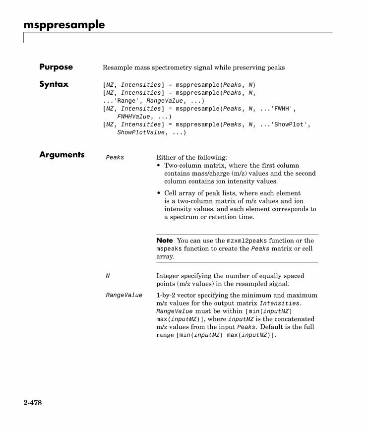
msppresample
Purpose Resample mass spectrometry signal while preserving peaks
Syntax [MZ, Intensities] = msppresample(Peaks, N)[MZ, Intensities] = msppresample(Peaks, N,...'Range', RangeValue, ...)[MZ, Intensities] = msppresample(Peaks, N, ...'FWHH',
FWHHValue, ...)[MZ, Intensities] = msppresample(Peaks, N, ...'ShowPlot',
ShowPlotValue, ...)
Arguments Peaks Either of the following:• Two-column matrix, where the first column
contains mass/charge (m/z) values and the secondcolumn contains ion intensity values.
• Cell array of peak lists, where each elementis a two-column matrix of m/z values and ionintensity values, and each element corresponds toa spectrum or retention time.
Note You can use the mzxml2peaks function or themspeaks function to create the Peaks matrix or cellarray.
N Integer specifying the number of equally spacedpoints (m/z values) in the resampled signal.
RangeValue 1-by-2 vector specifying the minimum and maximumm/z values for the output matrix Intensities.RangeValue must be within [min(inputMZ)max(inputMZ)], where inputMZ is the concatenatedm/z values from the input Peaks. Default is the fullrange [min(inputMZ) max(inputMZ)].
2-478

msppresample
FWHHValue Value that specifies the full width at half height(FWHH) in m/z units. The FWHH is used to converteach peak to a Gaussian shaped curve. Defaultis median(diff(inputMZ))/2, where inputMZ isthe concatenated m/z values from the input Peaks.The default is a rough approximation of resolutionobserved in the input data, Peaks.
Tip To ensure that the resolution of the peaksis preserved, set FWHHValue to half the distancebetween the two peaks of interest that are closest toeach other.
ShowPlotValue Controls the display of a plot of an original andresampled spectrum. Choices are true, false, orI, an integer specifying the index of a spectrum inIntensities. If set to true, the first spectrum inIntensities is plotted. Default is:
• false — When return values are specified.
• true — When return values are not specified.
ReturnValues
MZ Vector of equally spaced, common mass/charge (m/z)values for a set of spectra. The number of elements inthe vector equals N or the number of rows in matrixIntensities.
Intensities Matrix of reconstructed intensity values for a set ofmass spectra that share the same mass/charge (m/z)range. Each row corresponds to an m/z value, andeach column corresponds to a spectrum or retentiontime. The number of rows equals N or the numberof elements in vector MZ.
2-479
msppresample
Description [MZ, Intensities] = msppresample(Peaks, N) resamples Peaks,a mass spectrometry peak list, by converting centroided peaks to asemicontinuous, raw signal that preserves peak information. Theresampled signal has N equally spaced points. Output MZ is a vector ofN elements specifying the equally spaced, common m/z values for thespectra. Output Intensities is a matrix of reconstructed intensityvalues for a set of mass spectra that share the same m/z range. Eachrow corresponds to an m/z value, and each column corresponds to aspectrum or retention time. The number of rows equals N.
msppresample uses a Gaussian kernel to reconstruct the signal. The ionintensity at any given m/z value is taken from the maximum intensityof any contributing (overlapping) peaks.
Tip msppresample is useful to prepare a set of spectra for imagingfunctions such as msheatmap and preprocessing functions such asmsbackadj and msnorm.
[MZ, Intensities] = msppresample(Peaks, N,... 'PropertyName', PropertyValue, ...) calls msppresamplewith optional properties that use property name/property value pairs.You can specify one or more properties in any order. Each PropertyNamemust be enclosed in single quotation marks and is case insensitive.These property name/property value pairs are as follows:
[MZ, Intensities] = msppresample(Peaks, N, ...'Range',RangeValue, ...) specifies an m/z range for the output matrixIntensities using the minimum and maximum m/z valuesspecified in the 1-by-2 vector RangeValue. RangeValue must bewithin [min(inputMZ) max(inputMZ)], where inputMZ is theconcatenated m/z values from the input Peaks. Default is the full range[min(inputMZ) max(inputMZ)]
[MZ, Intensities] = msppresample(Peaks, N,...'FWHH', FWHHValue, ...) sets the full width at halfheight (FWHH) in m/z units. The FWHH is used to convert each peak
2-480

msppresample
to a Gaussian shaped curve. Default is median(diff(inputMZ))/2,where inputMZ is the concatenated m/z values from the input Peaks.The default is a rough approximation of resolution observed in theinput data, Peaks.
Tip To ensure that the resolution of the peaks is preserved, setFWHHValue to half the distance between the two peaks of interest thatare closest to each other.
[MZ, Intensities] = msppresample(Peaks, N,...'ShowPlot', ShowPlotValue, ...) controls the displayof a plot of an original and resampled spectrum. Choices aretrue, false, or I, an integer specifying the index of a spectrum inIntensities. If set to true, the first spectrum in Intensities isplotted. Default is:
• false — When return values are specified.
• true — When return values are not specified.
Examples 1 Load a MAT file, included with Bioinformatics Toolbox, whichcontains liquid chromatography/mass spectrometry (LC/MS) datavariables, including peaks, a cell array of peak lists, where eachelement is a two-column matrix of m/z values and ion intensityvalues, and each element corresponds to a spectrum or retention time.
load lcmsdata
2 Resample the data, specifying 5000 m/z values in the resampledsignal. Then create a heat map of the LC/MS data.
[MZ,Y] = msppresample(peaks,5000);msheatmap(MZ,ret_time,log(Y))
2-481

msppresample
3 Plot the reconstructed profile spectra between two retention times.
figuret1 = 3370;t2 = 3390;h = find(ret_time>t1 & ret_time<t2);[MZ,Y] = msppresample(peaks(h),10000);plot3(repmat(MZ,1,numel(h)),repmat(ret_time(h)',10000,1),Y)xlabel('Mass/Charge (M/Z)')ylabel('Retention Time')
2-482

msppresample
zlabel('Relative Intensity')
4 Resample the data to plot the Total Ion Chromatogram (TIC).
figure[MZ,Y] = msppresample(peaks,5000);plot(ret_time,sum(Y))title('Total Ion Chromatogram (TIC)')xlabel('Retention Time')ylabel('Relative Intensity')
2-483

msppresample
5 Resample the data to plot the Extracted Ion Chromatogram (XIC) inthe 450 to 500 m/z range.
figure[MZ,Y] = msppresample(peaks,5000,'Range',[450 500]);plot(ret_time,sum(Y))title('Extracted Ion Chromatogram (XIC) from 450 to 500 M/Z')xlabel('Retention Time')ylabel('Relative Intensity')
2-484
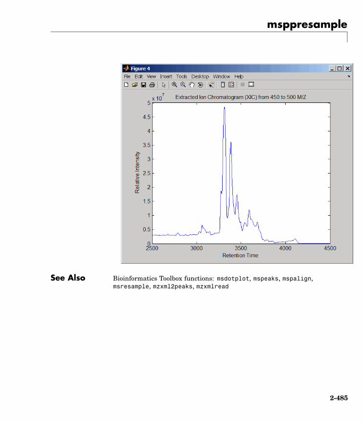
msppresample
See Also Bioinformatics Toolbox functions: msdotplot, mspeaks, mspalign,msresample, mzxml2peaks, mzxmlread
2-485

msresample
Purpose Resample mass spectrometry signal
Syntax [MZout, Yout] = msresample(MZ, Y, N)msresample(..., 'PropertyName', PropertyValue,...)msresample(..., 'Uniform', UniformValue)msresample(..., 'Range', RangeValue)msresample(..., 'Missing', MissingValue)msresample(..., 'Window', WindowValue)msresample(..., 'Cutoff', CutoffValue)msresample(..., 'ShowPlot', ShowPlotValue)
ArgumentsMZ Mass/charge vector with the range of ions in the
spectra.
Y Ion intensity vector with the same length as themass/charge vector (MZ). Y can also be a matrix withseveral spectra that share the same mass/charge (MZ)range.
N Total number of samples.
Description [MZout, Yout] = msresample(MZ, Y, N) resamples a raw massspectrum (Y). The output spectrum will have N samples with a spacingthat increases linearly within the range [min(MZ) max(MZ)]. MZ can bea linear or a quadratic function of its index. When input arguments areset such that down-sampling takes place, msresample applies a lowpassfilter before resampling to minimize aliasing.
For the antialias filter, msresample uses a linear-phase FIR filter witha least-squares error minimization. The cu-off frequency is set by thelargest down-sampling ratio when comparing the same regions in theMZ and MZout vectors.
Note msresample is particularly useful when you have spectra withdifferent mass/charge vectors and you want to match the scales.
2-486

msresample
msresample(..., 'PropertyName', PropertyValue,...) definesoptional properties using property name/value pairs.
msresample(..., 'Uniform', UniformValue), when UniformValue istrue, forces the vector MZ to be uniformly spaced. The default value isfalse.
msresample(..., 'Range', RangeValue) specifies a 1-by-2 vectorwith the mass/charge range for the output spectrum (Yout). RangeValuemust be within [min(MZ) max(MZ)]. The default value is the full range[min(MZ) max(MZ)].
msresample(..., 'Missing', MissingValue), when MissingValue istrue, analyzes the mass/charge vector (MZ) for dropped samples. Thedefault value is false. If the down-sample factor is large, checkingfor dropped samples might not be worth the extra computing time.Dropped samples can only be recovered if the original MZ values follow alinear or a quadratic function of the MZ vector index.
msresample(..., 'Window', WindowValue) specifies the window usedwhen calculating parameters for the lowpass filter. Enter 'Flattop','Blackman', 'Hamming’, or 'Hanning'. The default value is 'Flattop'.
msresample(..., 'Cutoff', CutoffValue) specifies the cutofffrequency. Enter a scalar value between 0 and 1 ( Nyquist frequencyor half the sampling frequency). By default, msresample estimatesthe cutoff value by inspecting the mass/charge vectors (MZ, MZout).However, the cutoff frequency might be underestimated if MZ hasanomalies.
msresample(..., 'ShowPlot', ShowPlotValue) plots the originaland the resampled spectrum. When msresample is called withoutoutput arguments, the spectra are plotted unless ShowPlotValue isfalse. When ShowPlotValue is true, only the first spectrum in Y isplotted. ShowPlotValue can also contain an index to one of the spectrain Y.
Examples 1 Load mass spectrometry data and extract m/z and intensity valuevectors
2-487

msresample
load sample_hi_res;mz = MZ_hi_res;y = Y_hi_res;
2 Plot original data to a lower resolution.
plot(mz, y, '.')
MATLAB draws a figure.
3 Resample data
[mz1,y1] = msresample(mz, y, 10000, 'range',[2000 max(mz)]);
4 Plot resampled data
plot(mz1,y1,'.')
MATLAB draws a figure with the down sampled data.
2-488

msresample
See Also Bioinformatics Toolbox functions: msalign, msbackadj, msheatmap,mslowess, msnorm, msppresample, mssgolay, msviewer
2-489
mssgolay
Purpose Smooth mass spectrum with least-squares polynomial
Syntax Yout = mssgolay(MZ, Y)mssgolay(..., 'PropertyName', PropertyValue,...)mssgolay(..., 'Span', SpanValue)mssgolay(..., 'Degree', DegreeValue)mssgolay(..., 'ShowPlot', ShowPlotValue)
ArgumentsMZ Mass/charge vector with the range of ions in the
spectra.
Y Ion intensity vector with the same length as themass/charge vector (MZ). Y can also be a matrix withseveral spectra that share the same mass/charge (MZ)range.
Description Yout = mssgolay(MZ, Y) smoothes a raw mass spectrum (Y) using aleast squares digital polynomial filter (Savitzky and Golay filters). Thedefault span or frame is 15 samples.
mssgolay(..., 'PropertyName', PropertyValue,...) definesoptional properties using property name/value pairs.
mssgolay(..., 'Span', SpanValue) modifies the frame size for thesmoothing function. If SpanValue is greater than 1, the window is thesize of SpanValue in samples independent of the MZ vector. Highervalues will smooth the signal more with an increase in computationtime. If SpanValue is less than 1, the window size is a fraction of thenumber of points in the data (MZ). For example, if SpanValue is 0.05,the window size is equal to 5% of the number of points in MZ.
2-490
mssgolay
Note 1) The original algorithm by Savitzky and Golay assumes auniformly spaced mass/charge vector (MZ), while mssgolay also allowsone that is not uniformly spaced. Therefore, the sliding frame forsmoothing is centered using the closest samples in terms of the MZ valueand not in terms of the MZ index.
2) When the vector MZ does not have repeated values or NaNs, thealgorithm is approximately twice as fast.
3) When the vector MZ is evenly spaced, the least-squares fittingis performed once so that the spectrum is filtered with the samecoefficients, and the speed of the algorithm increases considerably.
4) If the vector MZ is evenly spaced and SpanValue is even, Span isincriminated by 1 to include both edge samples in the frame.
mssgolay(..., 'Degree', DegreeValue) specifies the degree of thepolynomial (DegreeValue) fitted to the points in the moving frame. Thedefault value is 2. DegreeValue must be smaller than SpanValue.
mssgolay(..., 'ShowPlot', ShowPlotValue) plots smoothedspectra over the original. When mssgolay is called without outputarguments, the spectra are plotted unless ShowPlotValue is false.When ShowPlotValue is true, only the first spectrum in Y is plotted.ShowPlotValue can also contain an index to one of the spectra in Y.
Examples load sample_lo_resYS = mssgolay(MZ_low_res, Y_low_res(:,1));plot(MZ,[Y(:,1) YS])
See Also Bioinformatics Toolbox functions msalign, msbackadj, msheatmap,mslowess, msnorm, mspeaks, msresample, msviewer
2-491

msviewer
Purpose Explore mass spectrum or set of mass spectra
Syntax msviewer(MZ, Y)msviewer(..., 'Markers', MarkersValue)msviewer(..., 'Group', GroupValue)
ArgumentsMZ Mass/charge vector with the range of ions in the
spectra.
Y Ion intensity vector with the same length as themass/charge vector (MZ). Y can also be a matrix withseveral spectra that share the same mass/charge (MZ)range.
Description msviewer(MZ, Y) creates a GUI to display and explore a mass spectrum(Y).
msviewer(..., 'Markers', MarkersValue)specifies a list of markerpositions from the mass/charge vector (MZ) for exploration and easynavigation. Enter a column vector with MZ values.
msviewer(..., 'Group', GroupValue) specifies a class label forevery spectrum with a different color for every class. Enter a columnvector of size [numSpectra x 1] with integers. The default value is[numSpectra].
MSViewer GUI features include the following:
• Plot mass spectra. The spectra are plotted with different colorsaccording to their class labels.
• An overview displays a full spectrum, and a box indicates the regionthat is currently displayed in the main window.
• Five different zoom in options, one zoom out option, and a reset viewoption resize the spectrum.
• Add/focus/move/delete marker operations
2-492

msviewer
• Import/Export markers from/to MATLAB workspace
• Print and preview the spectra plot
• Print the spectra plot to a MATLAB figure window
MSViewer has five components:
• Menu bar: File, Tools, Window, and Help
• Toolbar: Zoom XY, Zoom X, Zoom Y, Reset view, Zoom out, and Help
• Main window: display the spectra
• Overview window: display the overview of a full spectrum (theaverage of all spectra in display)
• Marker control panel: a list of markers, Add marker, Delete marker,up and down buttons
Examples 1 Load and plot sample data
load sample_lo_resmsviewer(MZ_lo_res, Y_lo_res)
2 Add a marker by pointing to a mass peak, right-clicking, and thenclicking Add Marker.
3 From the File menu, select
• Import Markers from Workspace — Opens the Import MarkersFrom MATLAB Workspace dialog. The dialog should display a listof double Mx1 or 1xM variables. If the selected variable is out ofrange, the viewer displays an error message
• Export Markers to Workspace — Opens the Export Markers toMATLAB Workspace dialog. You can enter a variable name for themarkers. All markers are saved. If there is no marker available,this menu item should be disabled.
2-493

msviewer
• Print to Figure — Prints the spectra plot in the main display to aMATLAB figure window
4 From the Tools menu, click
• Add Marker — Opens the Add Marker dialog. Enter an m/zmarker.
• Delete Marker — Removes the currently selected m/z markerfrom the Markers (m/z) list.
• Next Marker or Previous Marker — Moves the selection up anddown the Markers (m/z) list.
• Zoom XY, Zoom X, Zoom Y, or Zoom Out — Changes the cursorfrom an arrow to crosshairs. Left-click and drag a rectangle boxover an area and then release the mouse button. The displayzooms the area covered by the box.
5 Move the cursor to the range window at the bottom. Click and dragthe view box to a new location.
See Also Bioinformatics Toolbox functions msalign, msbackadj, mslowess,msnorm, msheatmap, msresample, mssgolay
2-494

multialign
Purpose Align multiple sequences using progressive method
Syntax SeqsMultiAligned = multialign(Seqs)SeqsMultiAligned = multialign(Seqs, Tree)multialign(..., 'PropertyName', PropertyValue,...)multialign(..., 'Weights', WeightsValue)multialign(..., 'ScoringMatrix', ScoringMatrixValue)multialign(..., 'SMInterp', SMInterpValue)multialign(..., 'GapOpen', GapOpenValue)multialign(..., 'ExtendGap', ExtendGapValue)multialign(..., 'DelayCutoff', DelayCutoffValue)multialign(..., 'JobManager', JobManagerValue)multialign(..., 'WaitInQueue', WaitInQueueValue)multialign(..., 'Verbose', VerboseValue)multialign(..., 'ExistingGapAdjust',ExistingGapAdjustValue)multialign(..., 'TerminalGapAdjust',TerminalGapAdjustValue)
Arguments Seqs Vector of structures with the fields'Sequence' for the residues and'Header' or 'Name' for the labels.
Seqs may also be a cell array of stringsor a char array.
SeqsMultiAligned Vector of structures (same as Seqs) butwith the field 'Sequence' updated withthe alignment.
When Seqs is a cell or char array,SeqsMultiAligned is a char array withthe output alignment following thesame order as the input.
2-495
multialign
Tree Phylogenetic tree calculated witheither of the functions seqlinkage orseqneighjoin.
WeightsValue Property to select the sequenceweighting method. Enter either 'THG'(default) or 'equal'.
ScoringMatrixValue Property to select or specify thescoring matrix. Enter an [MxM]matrix or [MxMxN] array of matrixeswithN user-defined scoring matrices.ScoringMatrixValuemay also be a cellarray of strings with matrix names.Thedefault is the BLOSUM80 to BLOSUM30series for amino acids or a fixed matrixNUC44 for nucleotides. When passingyour own series of scoring matricesmake sure all of them share the samescale.
SMInterpValue Property to specify whether linearinterpolation of the scoring matrices ison or off. When false, scoring matrix isassigned to a fixed range depending onthe distances between the two profiles(or sequences) being aligned. Defaultis true.
GapOpenValue Scalar or a function specified using @. Ifyou enter a function,multialign passesfour values to the function: the averagescore for two matched residues (sm),the average score for two mismatchedresidues (sx), and, the length of bothprofiles or sequences (len1, len2).Default is @(sm,sx,len1,len2) 5*sm.
2-496

multialign
ExtendGapValue Scalar or a function specified using @.IF you enter a function, multiialignpasses four values to the function:the average score for two matchedresidues (sm), the average scorefor two mismatched residues (sx),and the length of both profiles orsequences (len1, len2). Default is@(sm,sx,len1,len2) sm/4.
DelayCutoffValue Property to specify the threshold delayof divergent sequences. The default isunity where sequences with the closestsequence farther than the mediandistance are delayed.
JobManagerValue JobManager object representingan available distributed MATLABresource. Enter a jobmanager objectreturned by the Distributed ComputingToolbox function findResource.
WaitInQueueValue Property to control waiting for adistributed MATLAB resource to beavailable. Enter either true or false.The default value is false.
VerboseValue Property to control displaying thesequences with sequence information.Default value is false.
ExistingGagAdjustValue Property to control automaticadjustment based on existing gaps.Default value is true.
TerminalGapAdjustValue Property to adjusts the penalty foropening a gap at the ends of thesequence. Default value is false.
2-497
multialign
Description SeqsMultiAligned = multialign(Seqs) performs a progressivemultiple alignment for a set of sequences (Seqs). Pair-wise distancesbetween sequences are computed after pair-wise alignment with theGonnet scoring matrix and then by counting the proportion of sites atwhich each pair of sequences are different (ignoring gaps). The guidetree is calculated by the neighbor-joining method assuming equalvariance and independence of evolutionary distance estimates.
SeqsMultiAligned = multialign(Seqs, Tree) uses a tree (Tree) asa guide for the progressive alignment. The sequences (Seqs) shouldhave the same order as the leaves in the tree (Tree) or use a field('Header' or 'Name') to identify the sequences.
multialign(..., 'PropertyName', PropertyValue,...) entersoptional arguments as property name/value pairs.
multialign(..., 'Weights', WeightsValue) selects the sequenceweighting method. Weights emphasize highly divergent sequences byscaling the scoring matrix and gap penalties. Closer sequences receivesmaller weights.
Values of the property Weights:
• 'THG'(default) — Thompson-Higgins-Gibson method using thephylogenetic tree branch distances weighted by their thickness.
• 'equal' — Assigns same weight to every sequence.
multialign(..., 'ScoringMatrix', ScoringMatrixValue)selects the scoring matrix (ScoringMatrixValue) for the progressivealignment. Match and mismatch scores are interpolated from theseries of scoring matrices by considering the distances between thetwo profiles or sequences being aligned. The first matrix correspondsto the smallest distance and the last matrix to the largest distance.Intermediate distances are calculated using linear interpolation.
multialign(..., 'SMInterp', SMInterpValue), whenSMInterpValue is false, turns off the linear interpolation of thescoring matrices. Instead, each supplied scoring matrix is assigned to
2-498

multialign
a fixed range depending on the distances between the two profiles orsequences being aligned.
multialign(..., 'GapOpen', GapOpenValue) specifies the initialpenalty for opening a gap.
multialign(..., 'ExtendGap', ExtendGapValue) specifies theinitial penalty for extending a gap.
multialign(..., 'DelayCutoff', DelayCutoffValue) specifies athreshold to delay the alignment of divergent sequences whose closestneighbor is farther than
(DelayCutoffValue) * (median patristic distancebetween sequences)
multialign(..., 'JobManager', JobManagerValue) distributespair-wise alignments into a cluster of computers using DistributedComputing Toolbox.
multialign(..., 'WaitInQueue', WaitInQueueValue) whenWaitInQueueValue is true, waits in the job manager queue for anavailable worker. When WaitInQueueValue is false (default) and thereare no workers immediately available, multialign errors out. Use thisproperty with Distributed Computing Toolbox and the multialignproperty WaitInQueue.
multialign(..., 'Verbose', VerboseValue), when VerboseValue istrue, turns on verbosity.
The remaining input optional arguments are analogous to the functionprofalign and are used through every step of the progressivealignment of profiles.
multialign(..., 'ExistingGapAdjust',ExistingGapAdjustValue), if ExistingGapAdjustValueis false, turns off the automatic adjustment based on existing gaps ofthe position-specific penalties for opening a gap.
When ExistingGapAdjustValue is true, for every profile position,profalign proportionally lowers the penalty for opening a gap toward
2-499
multialign
the penalty of extending a gap based on the proportion of gaps found inthe contiguous symbols and on the weight of the input profile.
multialign(..., 'TerminalGapAdjust',TerminalGapAdjustValue), when TerminalGapAdjustValue is true,adjusts the penalty for opening a gap at the ends of the sequence tobe equal to the penalty for extending a gap.
Example1 1 Align seven cellular tumor antigen p53 sequences.
p53 = fastaread('p53samples.txt')ma = multialign(p53,'verbose',true)showalignment(ma)
2-500

multialign
2 Use an UPGMA phylogenetic tree instead as a guiding tree.
dist = seqpdist(p53,'ScoringMatrix',gonnet);tree = seqlinkage(dist,'UPGMA',p53)
Phylogenetic tree object with 7 leaves (6 branches)
3 Score the progressive alignment with the PAM family.
ma = multialign(p53,tree,'ScoringMatrix',...{'pam150','pam200','pam250'})
showalignment(ma)
2-501
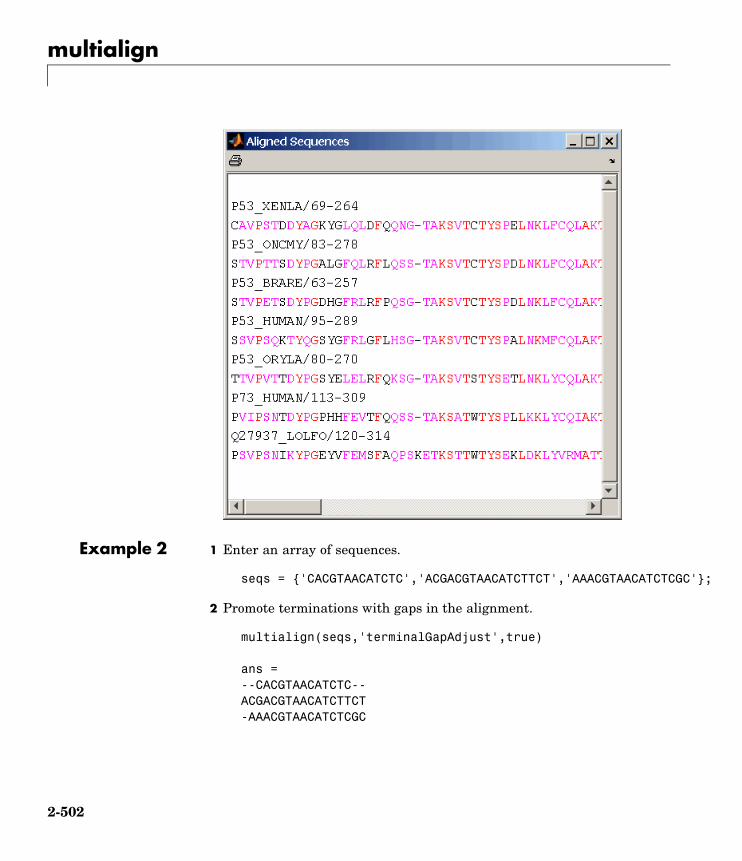
multialign
Example 2 1 Enter an array of sequences.
seqs = {'CACGTAACATCTC','ACGACGTAACATCTTCT','AAACGTAACATCTCGC'};
2 Promote terminations with gaps in the alignment.
multialign(seqs,'terminalGapAdjust',true)
ans =--CACGTAACATCTC--ACGACGTAACATCTTCT-AAACGTAACATCTCGC
2-502

multialign
3 Compare alignment without termination gap adjustment.
multialign(seqs)
ans =CA--CGTAACATCT--CACGACGTAACATCTTCTAA-ACGTAACATCTCGC
See Also Bioinformatics Toolbox functions: hmmprofalign, multialignread,nwalign, profalign, seqprofile, seqconsensus, seqneighjoin,showalignment
2-503

multialignread
Purpose Read multiple-sequence alignment file
Syntax S = multialignread(File)[Headers, Sequences] = multialignread(File)multialignread(..., 'PropertyName', PropertyValue,...)multialignread(..., 'IgnoreGaps', IgnoreGapsValue)
ArgumentsFile Multiple sequence alignment file (ASCII text
file). Enter a file name, a path and file name,or a URL pointing to a file. File can also be aMATLAB character array that contains the textof a multiple sequence alignment file. You canread common multiple alignment file types, suchas ClustalW (.aln) and GCG (.msf).
IgnoreGapsValue Property to control removing gap symbols.
Description S = multialignread(File) reads a multiple sequence alignment file.The file contains multiple sequence lines that start with a sequenceheader followed by an optional number (not used by multialignread)and a section of the sequence. The multiple sequences are broken intoblocks with the same number of blocks for every sequence. (For anexample, type open aagag.aln.) The output S is a structure arraywhere S.Header contains the header information and S.Sequencecontains the amino acid or nucleotide sequences.
[Headers, Sequences] = multialignread(File) reads the file intoseparate variables Headers and Sequences.
multialignread(..., 'PropertyName', PropertyValue,...)defines optional properties using property name/value pairs.
multialignread(..., 'IgnoreGaps', IgnoreGapsValue), whenIgnoreGapsValue is true, removes any gap symbol ('-' or '.') fromthe sequences. Default is false.
2-504

multialignread
Examples Read a multiple sequence alignment of the gag polyprotein for severalHIV strains.
gagaa = multialignread('aagag.aln')
gagaa =
1x16 struct array with fields:HeaderSequence
See Also Bioinformatics Toolbox functions: fastaread, gethmmalignment,multialign, seqconsensus, seqdisp, seqprofile
2-505

multialignviewer
Purpose Open viewer for multiple sequence alignments
Syntax multialignviewer(Alignment)multialignviewer(..., 'PropertyName', PropertyValue,...)multialignviewer(..., 'Alphabet', AlphabetValue)
Description The multialignviewer is an interactive graphical user interface (GUI)for viewing multiple sequence alignments.
multialignviewer(Alignment) loads a group of previously multiplealigned sequences into the viewer. Alignment is a structure with a fieldSequence, a character array, or a file name.
multialignviewer(..., 'PropertyName', PropertyValue,...)defines optional properties using property name/value pairs.
multialignviewer(..., 'Alphabet', AlphabetValue) specifiesthe alphabet type for the sequences . AlphabetValue can be 'AA'for amino acids or 'NT' for nucleotides. The default value is 'AA'.If AlphabetValue is not specified, multialignviewer guesses thealphabet type.
Examples multialignviewer('aagag.aln')
See Also Bioinformatics Toolbox functions: fastaread, gethmmalignment,multialign, multialignread, seqtool
2-506

mzxml2peaks
Purpose Convert mzXML structure to peak list
Syntax [Peaks, Times] = mzxml2peaks(mzXMLStruct)[Peaks, Times] = mzxml2peaks(mzXMLStruct,'Levels', LevelsValue)
ArgumentsmzXMLStruct mzXML structure, such as one created by the
mzxmlread function. mzXMLStruct includes thefollowing fields:
• scan
• offset
• mzXML
LevelsValue Positive integer or vector of integers that specifiesthe level(s) of spectra in mzXMLStruct to convert,assuming the spectra are from tandem MS data sets.Default is 1, which converts only the first-level spectra,that is spectra containing precursor ions. SettingLevelsValue to 2 converts only the second-levelspectra, which are the fragment spectra (created froma precursor ion).
2-507

mzxml2peaks
ReturnValues
Peaks Either of the following:• Two-column matrix, where the first column contains
mass/charge (m/z) values and the second columncontains ion intensity values.
• Cell array of peak lists, where each element is atwo-column matrix of m/z values and ion intensityvalues, and each element corresponds to a spectrumor retention time.
Times Vector of retention times associated with a liquidchromatography/mass spectrometry (LC/MS) or gaschromatography/mass spectrometry (GC/MS) data set.The number of elements in Times equals the numberof elements in Peaks.
Description [Peaks, Times] = mzxml2peaks(mzXMLStruct) extracts peakinformation from mzXMLStruct, an mzXML structure, and createsPeaks, a cell array of matrices containing mass/charge (m/z) values andion intensity values, and Times, a vector of retention times associatedwith a liquid chromatography/mass spectrometry (LC/MS) or gaschromatography/mass spectrometry (GC/MS) data set.
[Peaks, Times] = mzxml2peaks(mzXMLStruct,'Levels', LevelsValue) specifies the level(s) of the spectra inmzXMLStruct to convert, assuming the spectra are from tandem MSdata sets. Default is 1, which converts only the first-level spectra,that is spectra containing precursor ions. Setting LevelsValue to 2converts only the second-level spectra, which are the fragment spectra(created from a precursor ion).
Examples 1 Use the mzxmlread function to read an mzXML file into MATLAB asstructure. Then extract the peak information of only the first-levelions from the structure.
mzxml_struct = mzxmlread('results.mzxml');[peaks,time] = mzxml2peaks(mzxml_struct);
2-508
mzxml2peaks
Note The file results.mzxml is not provided. Sample mzXML filescan be found at
http://sashimi.sourceforge.net/repository.html
2 Create a dotplot of the LC/MS data.
msdotplot(peaks,time)
See Also Bioinformatics Toolbox functions: msdotplot, mspalign, msppresample,mzxmlread
2-509
mzxmlread
Purpose Read mzXML file into MATLAB as structure
Syntax mzXMLStruct = mzxmlread(File)
ArgumentsFile String containing a file name, or a path and file name,
of an mzXML file that conforms to the mzXML 2.1specification.
Description mzXMLStruct = mzxmlread(File) reads an mzXML file, File, andthen creates a MATLAB structure, mzXMLStruct.
File can be a file name, or a path and file name, of an mzXML file. Thefile must conform to the mzXML 2.1 specification at:
http://sashimi.sourceforge.net/schema_revision/mzXML_2.1/Doc/mzXML_2.1_tutorial.pdf
mzXMLStruct includes the following fields:
• scan
• offset
• mzXML
Tip If you receive any errors related to memory or Java heap space, tryincreasing your Java heap space as described at:
http://www.mathworks.com/support/solutions/data/1-18I2C.html
Examples out = mzxmlread('results.mzxml');% view a scanm = out.scan{1}.peaks.mz(1:2:end);z = out.scan{1}.peaks.mz(2:2:end);bar(m,z)
2-510
mzxmlread
Note The file results.mzxml is not provided. Sample mzXML filescan be found at:
http://sashimi.sourceforge.net/repository.html
See Also Bioinformatics Toolbox functions: jcampread, msdotplot, mslowess,msppresample, mssgolay, msviewer, mzxml2peaks
2-511
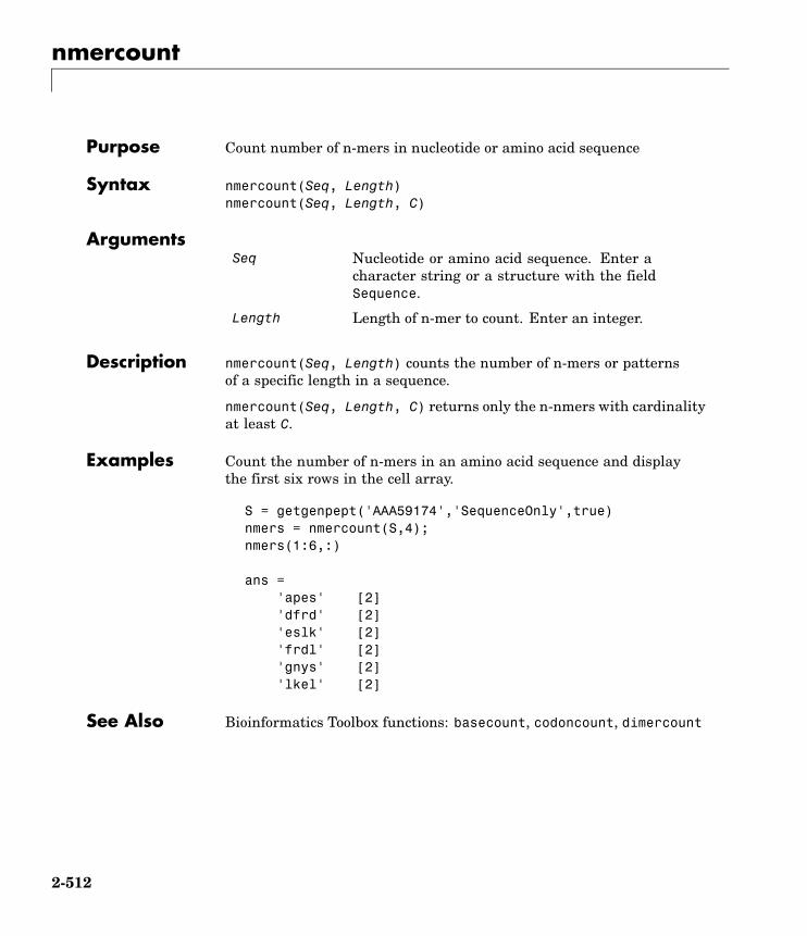
nmercount
Purpose Count number of n-mers in nucleotide or amino acid sequence
Syntax nmercount(Seq, Length)nmercount(Seq, Length, C)
ArgumentsSeq Nucleotide or amino acid sequence. Enter a
character string or a structure with the fieldSequence.
Length Length of n-mer to count. Enter an integer.
Description nmercount(Seq, Length) counts the number of n-mers or patternsof a specific length in a sequence.
nmercount(Seq, Length, C) returns only the n-nmers with cardinalityat least C.
Examples Count the number of n-mers in an amino acid sequence and displaythe first six rows in the cell array.
S = getgenpept('AAA59174','SequenceOnly',true)nmers = nmercount(S,4);nmers(1:6,:)
ans ='apes' [2]'dfrd' [2]'eslk' [2]'frdl' [2]'gnys' [2]'lkel' [2]
See Also Bioinformatics Toolbox functions: basecount, codoncount, dimercount
2-512
nt2aa
Purpose Convert nucleotide sequence to amino acid sequence
Syntax SeqAA = nt2aa(SeqNT)SeqAA = nt2aa(..., 'Frame', FrameValue, ...)SeqAA = nt2aa(..., 'GeneticCode', GeneticCodeValue, ...)SeqAA = nt2aa(..., 'AlternativeStartCodons',
AlternativeStartCodonsValue, ...)
2-513
nt2aa
Arguments SeqNT Either of the following:• String specifying a nucleotide
sequence
• MATLAB structure containingthe field Sequence
Valid characters include:
• A
• C
• G
• T
• U
• hyphen (-)
Note Hyphens are valid onlyif the codon to which it belongsrepresents a gap, that is, thecodon contains all hyphens.Example: ACT---TGA
Tip Do not use a sequence withhyphens if you specify 'all' forFrameValue.
FrameValue Property to specify a reading frame.Choices are 1, 2, 3, or 'all'. Defaultis 1.
If FrameValue is 'all', then SeqAAis a 3-by-1 cell array.
2-514
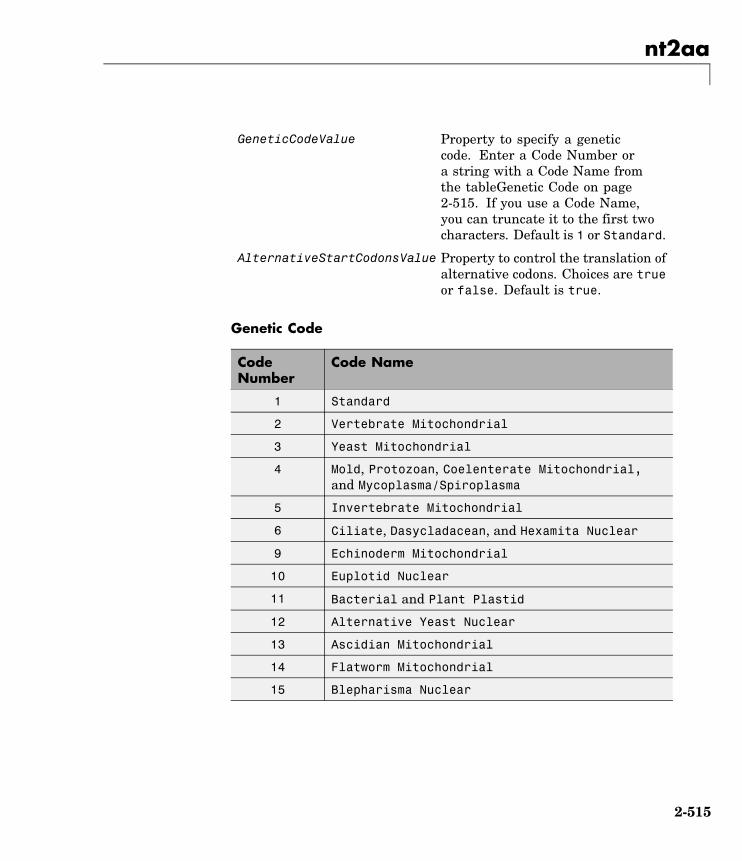
nt2aa
GeneticCodeValue Property to specify a geneticcode. Enter a Code Number ora string with a Code Name fromthe tableGenetic Code on page2-515. If you use a Code Name,you can truncate it to the first twocharacters. Default is 1 or Standard.
AlternativeStartCodonsValue Property to control the translation ofalternative codons. Choices are trueor false. Default is true.
Genetic Code
CodeNumber
Code Name
1 Standard
2 Vertebrate Mitochondrial
3 Yeast Mitochondrial
4 Mold, Protozoan, Coelenterate Mitochondrial,and Mycoplasma/Spiroplasma
5 Invertebrate Mitochondrial
6 Ciliate, Dasycladacean, and Hexamita Nuclear
9 Echinoderm Mitochondrial
10 Euplotid Nuclear
11 Bacterial and Plant Plastid
12 Alternative Yeast Nuclear
13 Ascidian Mitochondrial
14 Flatworm Mitochondrial
15 Blepharisma Nuclear
2-515

nt2aa
CodeNumber
Code Name
16 Chlorophycean Mitochondrial
21 Trematode Mitochondrial
22 Scenedesmus Obliquus Mitochondrial
23 Thraustochytrium Mitochondrial
ReturnValues
SeqAA String specifying an amino acidsequence.
Description SeqAA = nt2aa(SeqNT) converts a nucleotide sequence to an aminoacid sequence using the standard genetic code.
SeqAA = nt2aa(SeqNT, ...'PropertyName', PropertyValue, ...)calls nt2aa with optional properties that use property name/propertyvalue pairs. You can specify one or more properties in any order. EachPropertyName must be enclosed in single quotation marks and is caseinsensitive. These property name/property value pairs are as follows:
SeqAA = nt2aa(..., 'Frame', FrameValue, ...) converts anucleotide sequence for a specific reading frame to an amino acidsequence. Choices are 1, 2, 3, or 'all'. Default is 1. If FrameValue is'all', then output SeqAA is a 3-by-1 cell array.
SeqAA = nt2aa(..., 'GeneticCode', GeneticCodeValue, ...)converts a nucleotide sequence to an amino acid sequence using aspecific genetic code.
SeqAA = nt2aa(...,'AlternativeStartCodons', AlternativeStartCodonsValue, ...)controls the translation of alternative start codons. By default,AlternativeStartCodonsValue is set to true, and if the firstcodon of a sequence is a known alternative start codon, thecodon is translated to methionine.
2-516
nt2aa
If this option is set to false, then an alternative start codon at the startof a sequence is translated to its corresponding amino acid in the geneticcode that you specify, which might not necessarily be methionine. Forexample, in the human mitochondrial genetic code, AUA and AUU areknown to be alternative start codons.
For more details of alternative start codons, see
www.ncbi.nlm.nih.gov/Taxonomy/Utils/wprintgc.cgi?mode=t#SG1
Examples The following example converts the gene ND1 on the humanmitochondria genome to an amino acid sequence.
mitochondria = getgenbank('NC_001807', 'SequenceOnly', true)ND1gene = mitochondria (3308:4264)protein1 = nt2aa(ND1gene,'GeneticCode', 2)protein2 = getgenpept('NP_536843', 'SequenceOnly', true)
The following example converts the gene ND2 on the humanmitochondria genome to an amino acid sequence. In this case, the firstcodon is ATT, which is translated to M, while the following ATT codonsare converted to I. If you set 'AlternativeStartCodons' to false,then the first codon ATT is translated to I, the corresponding amino acidin the Vertebrate Mitochondrial genetic code.
mitochondria = getgenbank('NC_001807', 'SequenceOnly', true)ND2gene = mitochondria (4471:5514)protein1 = nt2aa(ND2gene, 'GeneticCode', 2)protein2 = getgenpept('NP_536844', 'SequenceOnly', true)
See Also Bioinformatics Toolbox functions: aa2int, aminolookup, baselookup,codonbias, dnds, dndsml, geneticcode, revgeneticcode, seqtool
2-517

nt2int
Purpose Convert nucleotide sequence from letter to integer representation
Syntax SeqInt = nt2int(SeqChar, 'PropertyName', PropertyValue)nt2int(..., 'Unknown', UnknownValue)nt2int(..., 'ACGTOnly', ACGTONlyValue)
ArgumentsSeqChar Nucleotide sequence represented with letters.
Enter a character string from the table MappingNucleotide Letters to Integers below. Integersare arbitrarily assigned to IUB/IUPAC letters.If the property ACGTOnly is true, you can onlyenter the characters A, C, T, G, and U.
UnknownValue Property to select the integer for unknowncharacters. Enter an integer. Maximum value is255. Default value is 0.
ACGTOnlyValue Property to control the use of ambiguousnucleotides. Enter either true or false. Defaultvalue is false.
Mapping Nucleotide Letters to Integers
Base Code Base Code Base Code
Adenosine A—1 T, C(pyrimidine)
Y—6 A, T, G (notC)
D—12
Cytidine C—2 G, T (keto) K—7 A, T, C (notG)
H—13
Guanine G—3 A, C (amino) M—8 A, G, C (notT)
V—14
Thymidine T—4 G, C (strong) S—9 A, T, G, C (any) N—15
2-518

nt2int
Base Code Base Code Base Code
Uridine U—4 A, T (weak) W—10 Gap ofindeterminatelength
- —16
A, G(purine)
R—5 T, G, C (notA)
B—11 Unknown(default)
*—0and≥17
Description SeqInt = nt2int(SeqChar, 'PropertyName', PropertyValue) convertsa character string of nucleotides to a 1-by-N array of integers usingthe table Mapping Nucleotide Letters to Integers above. Unknowncharacters (characters not in the table) are mapped to 0. Gapsrepresented with hyphens are mapped to 16.
nt2int(..., 'Unknown', UnknownValue) defines the number used torepresent unknown nucleotides. The default value is 0.
nt2int(..., 'ACGTOnly', ACGTONlyValue) if ACGTOnly is true, theambiguous nucleotide characters (N, R, Y, K, M, S, W, B, D, H, and V) arerepresented by the unknown nucleotide number.
Examples Convert a nucleotide sequence with letters to integers.
s = nt2int('ACTGCTAGC')
s =1 2 4 3 2 4 1 3 2
See Also Bioinformatics Toolbox functions: aa2int, baselookup, int2aa, int2nt
2-519

ntdensity
Purpose Plot density of nucleotides along sequence
Syntax Density = ntdensity(SeqNT, 'PropertyName', PropertyValue)ntdensity(..., 'Window', WindowValue)[Density, HighCG] = ntdensity(..., 'CGThreshold',
CGThresholdValue)
Description ntdensity(SeqNT) plots the density of nucleotides A, T, C, G in sequenceSeqNT.
Density = ntdensity(SeqNT, 'PropertyName', PropertyValue) returnsa MATLAB structure with the density of nucleotides A, C, G, and T.
ntdensity(..., 'Window', WindowValue) uses a window oflength Window for the density calculation. The default value islength(SeqNT)/20.
[Density, HighCG] = ntdensity(..., 'CGThreshold',CGThresholdValue) returns indices for regions where the CG content ofSeqNT is greater than CGThreshold. The default value for CGThresholdis 5.
Examples s = randseq(1000, 'alphabet', 'dna');ndensity(s)
2-520
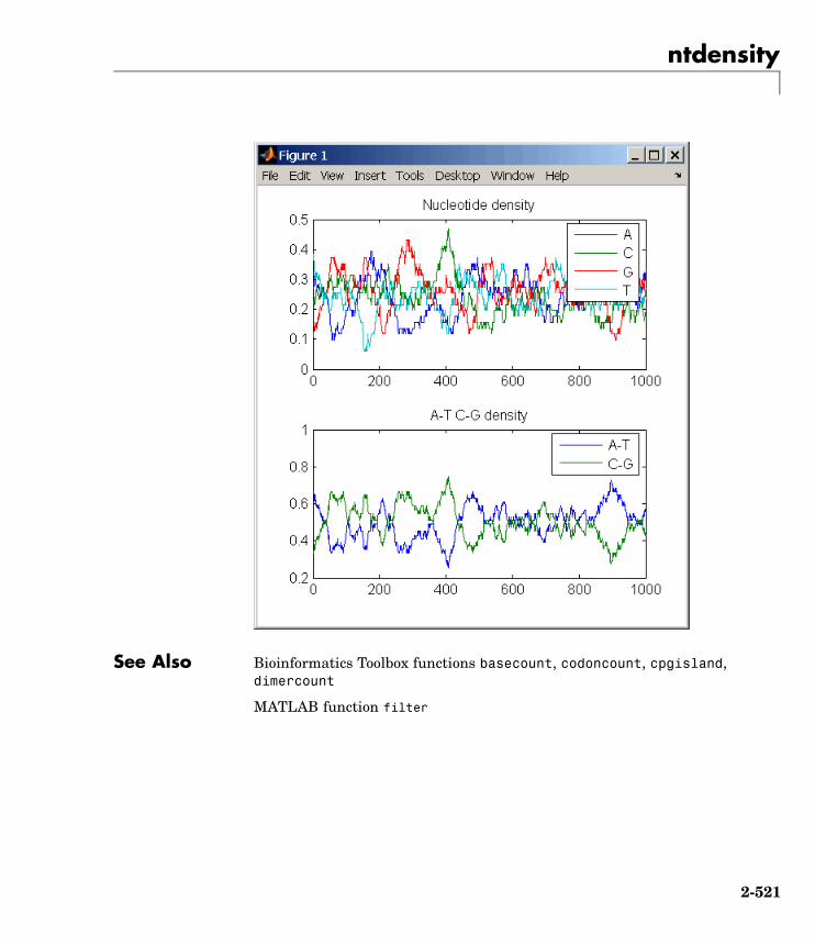
ntdensity
See Also Bioinformatics Toolbox functions basecount, codoncount, cpgisland,dimercount
MATLAB function filter
2-521
nuc44
Purpose NUC44 scoring matrix for nucleotide sequences
Syntax ScoringMatrix = nuc44[ScoringMatrix, MatrixInfo] = nuc44
Description ScoringMatrix = nuc44 returns the scoring matrix. The nuc44 scoringmatrix uses ambiguous nucleotide codes and probabilities rounded tothe nearest integer.
Scale = 0.277316
Expected score = -1.7495024, Entropy = 0.5164710 bits
Lowest score = -4, Highest score = 5
Order: A C G T R Y K M S W B D H V N
[ScoringMatrix, MatrixInfo] = nuc44 returns a structure withinformation about the matrix with fields Name and Order.
2-522

num2goid
Purpose Convert numbers to Gene Ontology IDs
Syntax GOIDs = num2goid(X)
Description GOIDs = num2goid(X) converts the numbers in X to strings with GeneOntology IDs. IDs are a 7-digit number preceded by the prefix 'GO:'.
Examples Get the Gene Ontology IDs of the following numbers.
t = [5575 5622 5623 5737 5840 30529 43226 43228 ...43229 43232 43234];
ids = num2goid(t)
See Also Bioinformatics Toolbox functions: geneont (object constructor),goannotread
Bioinformatics Toolbox methods of geneont object: getancestors,getdescendants, getmatrix, getrelatives
2-523
nwalign
Purpose Globally align two sequences using Needleman-Wunsch algorithm
Syntax Score = nwalign(Seq1,Seq2)[Score, Alignment] = nwalign(Seq1,Seq2)[Score, Alignment, Start] = nwalign(Seq1,Seq2)... = nwalign(Seq1,Seq2, ...'Alphabet', AlphabetValue, ...)... = nwalign(Seq1,Seq2, ...'ScoringMatrix',
ScoringMatrixValue, ...)... = nwalign(Seq1,Seq2, ...'Scale', ScaleValue, ...)... = nwalign(Seq1,Seq2, ...'GapOpen', GapOpenValue, ...)... = nwalign(Seq1,Seq2, ...'ExtendGap',ExtendGapValue, ...)... = nwalign(Seq1,Seq2, ...'Showscore',ShowscoreValue, ...)
Arguments Seq1, Seq2 Amino acid or nucleotide sequences. Enterany of the following:• Character string of letters representing
amino acids or nucleotides, such as returnedby int2aa or int2nt
• Vector of integers representing amino acidsor nucleotides, such as returned by aa2intor nt2int
• Structure containing a Sequence field
Tip For help with letter and integerrepresentations of amino acids andnucleotides, see Amino Acid Lookup Table onpage 2-42 or Nucleotide Lookup Table on page2-52.
AlphabetValue String specifying the type of sequence. Choicesare 'AA' (default) or 'NT'.
2-524

nwalign
ScoringMatrixValue String specifying the scoring matrix to use forthe global alignment. Choices for amino acidsequences are:
• 'PAM40'
• 'PAM250'
• 'DAYHOFF'
• 'GONNET'
• 'BLOSUM30' increasing by 5 up to'BLOSUM90'
• 'BLOSUM62'
• 'BLOSUM100'
Default is:
• 'BLOSUM50' (when AlphabetValue equals'AA')
• 'NUC44' (when AlphabetValue equals'NT')
Note All of the above scoring matrices have abuilt-in scale factor that returns Score in bits.
ScaleValue Positive value that specifies the scale factorused to return Score in arbitrary units otherthan bits. For example, if you enter log(2)for ScaleValue, then nwalign returns Scorein nats.
GapOpenValue Positive integer specifying the penalty foropening a gap in the alignment. Default is 8.
2-525

nwalign
ExtendGapValue Positive integer specifying the penaltyfor extending a gap. Default is equal toGapOpenValue.
ShowscoreValue Controls the display of the scoring space andthe winning path of the alignment. Choicesare true or false (default).
ReturnValues
Score Optimal global alignment score in bits.
Alignment 3-by-N character array showing the twosequences, Seq1 and Seq2, in the first andthird rows, and symbols representing theoptimal global alignment for them in thesecond row.
Start 2-by-1 vector of indices indicating the startingpoint in each sequence for the alignment.Because this is a global alignment, Start isalways [1;1].
Description Score = nwalign(Seq1,Seq2) returns the optimal global alignmentscore in bits. The scale factor used to calculate the score is provided bythe scoring matrix.
[Score, Alignment] = nwalign(Seq1,Seq2) returns a 3-by-Ncharacter array showing the two sequences, Seq1 and Seq2, in thefirst and third rows, and symbols representing the optimal globalalignment for them in the second row. The symbol | indicates aminoacids or nucleotides that match exactly. The symbol : indicates aminoacids or nucleotides that are related as defined by the scoring matrix(nonmatches with a zero or positive scoring matrix value).
[Score, Alignment, Start] = nwalign(Seq1,Seq2) returns a 2-by-1vector of indices indicating the starting point in each sequence for thealignment. Because this is a global alignment, Start is always [1;1].
2-526

nwalign
... = nwalign(Seq1,Seq2, ...'PropertyName',PropertyValue, ...) calls nwalign with optional propertiesthat use property name/property value pairs. You can specify one ormore properties in any order. Each PropertyName must be enclosedin single quotation marks and is case insensitive. These propertyname/property value pairs are as follows:
... = nwalign(Seq1,Seq2, ...'Alphabet',AlphabetValue, ...) specifies the type of sequences. Choices are'AA' (default) or 'NT'.
... = nwalign(Seq1,Seq2,
...'ScoringMatrix', ScoringMatrixValue, ...) specifies thescoring matrix to use for the global alignment. Default is:
• 'BLOSUM50' (when AlphabetValue equals 'AA')
• 'NUC44' (when AlphabetValue equals 'NT')
... = nwalign(Seq1,Seq2, ...'Scale', ScaleValue, ...)specifies the scale factor used to return Score in arbitrary units otherthan bits. Choices are any positive value.
... = nwalign(Seq1,Seq2, ...'GapOpen', GapOpenValue, ...)specifies the penalty for opening a gap in the alignment. Choices areany positive integer. Default is 8.
... = nwalign(Seq1,Seq2, ...'ExtendGap',ExtendGapValue, ...) specifies the penalty for extending a gapin the alignment. Choices are any positive integer. Default is equalto GapOpenValue.
... = nwalign(Seq1,Seq2, ...'Showscore',ShowscoreValue, ...) controls the display of the scoring space andwinning path of the alignment. Choices are true or false (default)
2-527
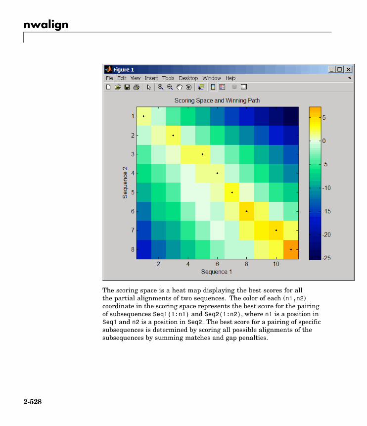
nwalign
The scoring space is a heat map displaying the best scores for allthe partial alignments of two sequences. The color of each (n1,n2)coordinate in the scoring space represents the best score for the pairingof subsequences Seq1(1:n1) and Seq2(1:n2), where n1 is a position inSeq1 and n2 is a position in Seq2. The best score for a pairing of specificsubsequences is determined by scoring all possible alignments of thesubsequences by summing matches and gap penalties.
2-528
nwalign
The winning path is represented by black dots in the scoring space andrepresents the pairing of positions in the optimal global alignment. Thecolor of the last point (lower right) of the winning path represents theoptimal global alignment score for the two sequences and is the Scoreoutput returned by nwalign.
Tip The scoring space visually indicates if there are potential alternatewinning paths, which is useful when aligning sequences with biggaps. Visual patterns in the scoring space can also indicate a possiblesequence rearrangement.
Examples 1 Globally align two amino acid sequences using the BLOSUM50 (default)scoring matrix and the default values for the GapOpen and ExtendGapproperties. Return the optimal global alignment score in bits andthe alignment character array.
[Score, Alignment] = nwalign('VSPAGMASGYD','IPGKASYD')
Score =
7.3333
Alignment =
VSPAGMASGYD: | | || ||I-P-GKAS-YD
2 Globally align two amino acid sequences specifying the PAM250scoring matrix and a gap open penalty of 5.
[Score, Alignment] = nwalign('IGRHRYHIGG','SRYIGRG',...'scoringmatrix','pam250',...'gapopen',5)
2-529
nwalign
Score =
2.3333
Alignment =
IGRHRYHIG-G: || || |
-S--RY-IGRG
3 Globally align two amino acid sequences returning the Score in natunits (nats) by specifying a scale factor of log(2).
[Score, Alignment] = nwalign('HEAGAWGHEE','PAWHEAE','Scale',log(2))
Score =
0.2310
Alignment =
HEAGAWGHE-E
|| || |
--P-AW-HEAE
References [1] Durbin, R., Eddy, S., Krogh, A., and Mitchison, G. (1998). BiologicalSequence Analysis (Cambridge University Press).
See Also Bioinformatics Toolbox functions: blosum, multialign, nt2aa, pam,profalign, seqdotplot, showalignment, swalign
2-530
oligoprop
Purpose Calculate sequence properties of DNA oligonucleotide
Syntax SeqProperties = oligoprop(SeqNT)SeqProperties = oligoprop(SeqNT, ...'Salt', SaltValue, ...)SeqProperties = oligoprop(SeqNT, ...'Temp', TempValue, ...)SeqProperties = oligoprop(SeqNT, ...'Primerconc',
PrimerconcValue, ...)SeqProperties = oligoprop(SeqNT, ...'HPBase', HPBaseValue,
...)SeqProperties = oligoprop(SeqNT, ...'HPLoop', HPLoopValue,
...)SeqProperties = oligoprop(SeqNT, ...'Dimerlength',
DimerlengthValue, ...)
Arguments SeqNT DNA oligonucleotide sequence represented byany of the following:• Character string containing the letters A, C, G,
T, or N
• Vector of integers containing the integers 1,2, 3, 4, or 15
• Structure containing a Sequence field thatcontains a nucleotide sequence
SaltValue Value that specifies a salt concentration inmoles/liter for melting temperature calculations.Default is 0.05 moles/liter.
TempValue Value that specifies the temperature in degreesCelsius for nearest-neighbor calculations of freeenergy. Default is 25 degrees Celsius.
PrimerconcValue Value that specifies the concentration inmoles/liter for melting temperature calculations.Default is 50e-6 moles/liter.
2-531

oligoprop
HPBaseValue Value that specifies the minimum number ofpaired bases that form the neck of the hairpin.Default is 4 base pairs.
HPLoopValue Value that specifies the minimum number ofbases that form the loop of a hairpin. Default is2 bases.
DimerlengthValue Value that specifies the minimum number ofaligned bases between the sequence and itsreverse. Default is 4 bases.
ReturnValues
SeqProperties Structure containing the sequence properties fora DNA oligonucleotide.
Description SeqProperties = oligoprop(SeqNT) returns the sequence propertiesfor a DNA oligonucleotide as a structure with the following fields:
Field Description
GC Percent GC content for the DNA oligonucleotide.Ambiguous N characters in SeqNT are consideredto potentially be any nucleotide. If SeqNT containsambiguous N characters, GC is the midpoint value,and its uncertainty is expressed by GCdelta.
GCdelta The difference between GC (midpoint value) andeither the maximum or minimum value GC couldassume. The maximum and minimum values arecalculated by assuming all N characters are G/C ornot G/C, respectively. Therefore, GCdelta definesthe possible range of GC content.
2-532

oligoprop
Field Description
Hairpins H-by-length(SeqNT) matrix of charactersdisplaying all potential hairpin structures for thesequence SeqNT. Each row is a potential hairpinstructure of the sequence, with the hairpinforming nucleotides designated by capital letters.H is the number of potential hairpin structures forthe sequence. Ambiguous N characters in SeqNTare considered to potentially complement anynucleotide.
Dimers D-by-length(SeqNT) matrix of charactersdisplaying all potential dimers for the sequenceSeqNT. Each row is a potential dimer of thesequence, with the self-dimerizing nucleotidesdesignated by capital letters. D is the number ofpotential dimers for the sequence. Ambiguous Ncharacters in SeqNT are considered to potentiallycomplement any nucleotide.
MolWeight Molecular weight of the DNA oligonucleotide.Ambiguous N characters in SeqNT are consideredto potentially be any nucleotide. If SeqNT containsambiguous N characters, MolWeight is themidpoint value, and its uncertainty is expressedby MolWeightdelta.
MolWeightdelta The difference between MolWeight (midpointvalue) and either the maximum or minimumvalue MolWeight could assume. The maximumand minimum values are calculated by assumingall N characters are G or C, respectively. Therefore,MolWeightdelta defines the possible range ofmolecular weight for SeqNT.
2-533
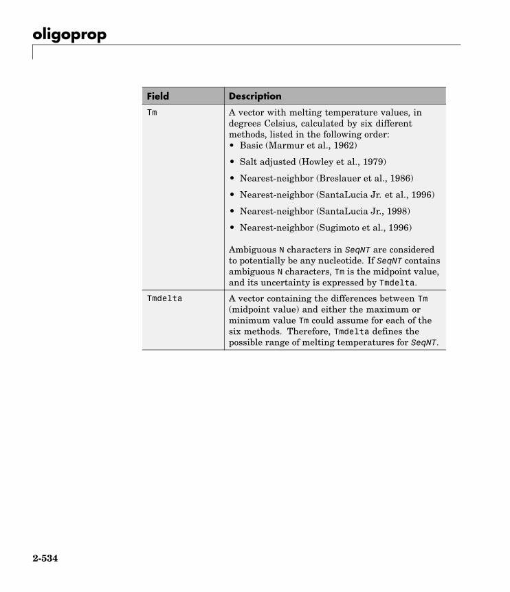
oligoprop
Field Description
Tm A vector with melting temperature values, indegrees Celsius, calculated by six differentmethods, listed in the following order:• Basic (Marmur et al., 1962)
• Salt adjusted (Howley et al., 1979)
• Nearest-neighbor (Breslauer et al., 1986)
• Nearest-neighbor (SantaLucia Jr. et al., 1996)
• Nearest-neighbor (SantaLucia Jr., 1998)
• Nearest-neighbor (Sugimoto et al., 1996)
Ambiguous N characters in SeqNT are consideredto potentially be any nucleotide. If SeqNT containsambiguous N characters, Tm is the midpoint value,and its uncertainty is expressed by Tmdelta.
Tmdelta A vector containing the differences between Tm(midpoint value) and either the maximum orminimum value Tm could assume for each of thesix methods. Therefore, Tmdelta defines thepossible range of melting temperatures for SeqNT.
2-534

oligoprop
Field Description
Thermo 4-by-3 matrix of thermodynamic calculations.
The rows correspond to nearest-neighborparameters from:
• Breslauer et al., 1986
• SantaLucia Jr. et al., 1996
• SantaLucia Jr., 1998
• Sugimoto et al., 1996
The columns correspond to:
• delta H — Enthalpy in kilocalories per mole,kcal/mol
• delta S — Entropy in calories per mole-degreesKelvin, cal/(K)(mol)
• delta G — Free energy in kilocalories per mole,kcal/mol
Ambiguous N characters in SeqNT are consideredto potentially be any nucleotide. If SeqNT containsambiguous N characters, Thermo is the midpointvalue, and its uncertainty is expressed byThermodelta.
Thermodelta 4-by-3 matrix containing the differences betweenThermo (midpoint value) and either the maximumor minimum value Thermo could assume for eachcalculation and method. Therefore, Thermodeltadefines the possible range of thermodynamicvalues for SeqNT.
SeqProperties = oligoprop(SeqNT, ...'PropertyName',PropertyValue, ...) calls oligoprop with optional properties that
2-535

oligoprop
use property name/property value pairs. You can specify one or moreproperties in any order. Each PropertyName must be enclosed in singlequotation marks and is case insensitive. These property name/propertyvalue pairs are as follows:
SeqProperties = oligoprop(SeqNT, ...'Salt', SaltValue, ...)specifies a salt concentration in moles/liter for melting temperaturecalculations. Default is 0.05 moles/liter.
SeqProperties = oligoprop(SeqNT, ...'Temp', TempValue, ...)specifies the temperature in degrees Celsius for nearest-neighborcalculations of free energy. Default is 25 degrees Celsius.
SeqProperties = oligoprop(SeqNT, ...'Primerconc',PrimerconcValue, ...) specifies the concentration in moles/liter formelting temperatures. Default is 50e-6 moles/liter.
SeqProperties = oligoprop(SeqNT, ...'HPBase', HPBaseValue,...) specifies the minimum number of paired bases that form the neckof the hairpin. Default is 4 base pairs.
SeqProperties = oligoprop(SeqNT, ...'HPLoop', HPLoopValue,...) specifies the minimum number of bases that form the loop of ahairpin. Default is 2 bases.
SeqProperties = oligoprop(SeqNT, ...'Dimerlength',DimerlengthValue, ...) specifies the minimum number of alignedbases between the sequence and its reverse. Default is 4 bases.
Examples Calculating Properties for a DNA Sequence
1 Create a random sequence.
seq = randseq(25)
seq =
TAGCTTCATCGTTGACTTCTACTAA
2 Calculate sequence properties of the sequence.
2-536
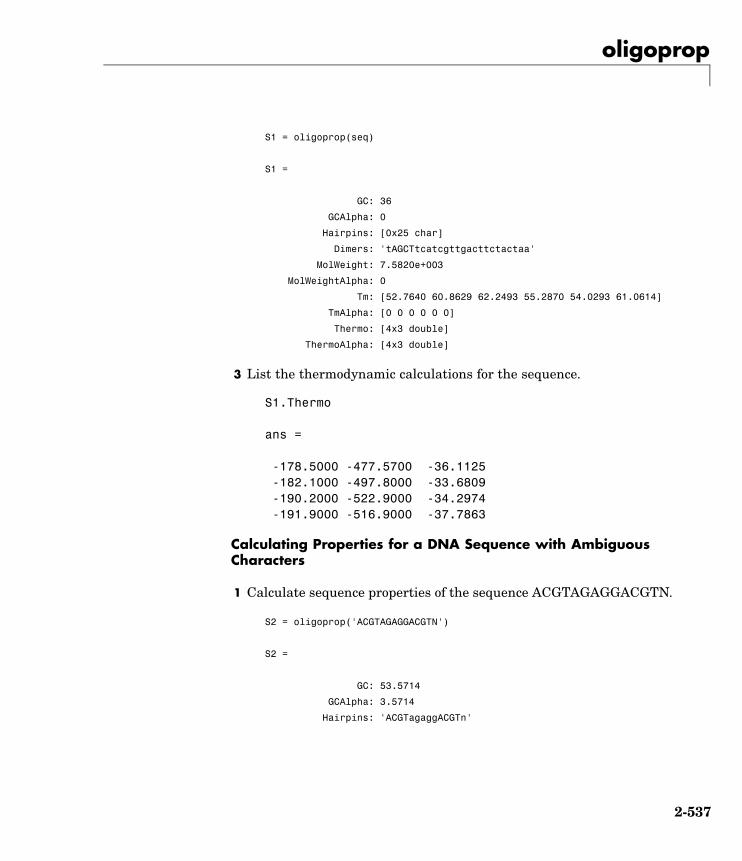
oligoprop
S1 = oligoprop(seq)
S1 =
GC: 36
GCAlpha: 0
Hairpins: [0x25 char]
Dimers: 'tAGCTtcatcgttgacttctactaa'
MolWeight: 7.5820e+003
MolWeightAlpha: 0
Tm: [52.7640 60.8629 62.2493 55.2870 54.0293 61.0614]
TmAlpha: [0 0 0 0 0 0]
Thermo: [4x3 double]
ThermoAlpha: [4x3 double]
3 List the thermodynamic calculations for the sequence.
S1.Thermo
ans =
-178.5000 -477.5700 -36.1125-182.1000 -497.8000 -33.6809-190.2000 -522.9000 -34.2974-191.9000 -516.9000 -37.7863
Calculating Properties for a DNA Sequence with AmbiguousCharacters
1 Calculate sequence properties of the sequence ACGTAGAGGACGTN.
S2 = oligoprop('ACGTAGAGGACGTN')
S2 =
GC: 53.5714
GCAlpha: 3.5714
Hairpins: 'ACGTagaggACGTn'
2-537

oligoprop
Dimers: [3x14 char]
MolWeight: 4.3329e+003
MolWeightAlpha: 20.0150
Tm: [38.8357 42.2958 57.7880 52.4180 49.9633 55.1330]
TmAlpha: [1.4643 1.4643 10.3885 3.4633 0.2829 3.8074]
Thermo: [4x3 double]
ThermoAlpha: [4x3 double]
2 List the potential dimers for the sequence.
S2.Dimers
ans =
ACGTagaggacgtnACGTagaggACGTnacgtagagGACGTN
References [1] Breslauer, K.J., Frank, R., Blöcker, H., and Marky, L.A. (1986).Predicting DNA duplex stability from the base sequence. Proceedings ofthe National Academy of Science USA 83, 3746–3750.
[2] Chen, S.H., Lin, C.Y., Cho, C.S., Lo, C.Z., and Hsiung, C.A. (2003).Primer Design Assistant (PDA): A web-based primer design tool.Nucleic Acids Research 31(13), 3751–3754.
[3] Howley, P.M., Israel, M.A., Law, M., and Martin, M.A. (1979). Arapid method for detecting and mapping homology between heterologousDNAs. Evaluation of polyomavirus genomes. The Journal of BiologicalChemistry 254(11), 4876–4883.
[4] Marmur, J., and Doty, P. (1962). Determination of the basecomposition of deoxyribonucleic acid from its thermal denaturationtemperature. Journal Molecular Biology 5, 109–118.
2-538

oligoprop
[5] Panjkovich, A., and Melo, F. (2005). Comparison of differentmelting temperature calculation methods for short DNA sequences.Bioinformatics 21(6), 711–722.
[6] SantaLucia Jr., J., Allawi, H.T., and Seneviratne, P.A. (1996).Improved Nearest-Neighbor Parameters for Predicting DNA DuplexStability. Biochemistry 35, 3555–3562.
[7] SantaLucia Jr., J. (1998). A unified view of polymer, dumbbell, andoligonucleotide DNA nearest-neighbor thermodynamics. Proceedings ofthe National Academy of Science USA 95, 1460–1465.
[8] Sugimoto, N., Nakano, S., Yoneyama, M., and Honda, K. (1996).Improved thermodynamic parameters and helix initiation factor topredict stability of DNA duplexes. Nucleic Acids Research 24(22),4501–4505.
[9] http://www.basic.northwestern.edu/biotools/oligocalc.html for weightcalculations.
See Also Bioinformatics Toolbox functions: isoelectric, molweight, ntdensity,palindromes, randseq
2-539
optimalleaforder
Purpose Determine optimal leaf ordering for hierarchical binary cluster tree
Syntax Order = optimalleaforder(Tree, Dist)Order = optimalleaforder(Tree, Dist, ...'Criteria',CriteriaValue, ...)Order = optimalleaforder(Tree, Dist, ...'Transformation',
TransformationValue, ...)
Arguments Tree Hierarchical binary cluster tree representedby an (M - 1)-by-3 matrix, created by thelinkage function, where M is the number ofleaves.
Dist Distance matrix, such as that created by thepdist function.
2-540
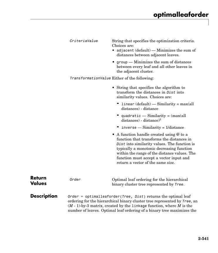
optimalleaforder
CriteriaValue String that specifies the optimization criteria.Choices are:• adjacent (default) — Minimizes the sum of
distances between adjacent leaves.
• group — Minimizes the sum of distancesbetween every leaf and all other leaves inthe adjacent cluster.
TransformationValue Either of the following:
• String that specifies the algorithm totransform the distances in Dist intosimilarity values. Choices are:
- linear (default) — Similarity = max(alldistances) - distance
- quadratic — Similarity = (max(alldistances) - distance)2
- inverse — Similarity = 1/distance
• A function handle created using @ to afunction that transforms the distances inDist into similarity values. The function istypically a monotonic decreasing functionwithin the range of the distance values. Thefunction must accept a vector input andreturn a vector of the same size.
ReturnValues
Order Optimal leaf ordering for the hierarchicalbinary cluster tree represented by Tree.
Description Order = optimalleaforder(Tree, Dist) returns the optimal leafordering for the hierarchical binary cluster tree represented by Tree, an(M - 1)-by-3 matrix, created by the linkage function, where M is thenumber of leaves. Optimal leaf ordering of a binary tree maximizes the
2-541
optimalleaforder
similarity between adjacent elements (clusters or leaves) by flippingtree branches, but without dividing the clusters. The input Dist is adistance matrix, such as that created by the pdist function.
Order = optimalleaforder(Tree, Dist, ...'PropertyName',PropertyValue, ...) calls optimalleaforder with optionalproperties that use property name/property value pairs. You canspecify one or more properties in any order. Each PropertyName mustbe enclosed in single quotation marks and is case insensitive. Theseproperty name/property value pairs are as follows:
Order = optimalleaforder(Tree, Dist, ...'Criteria',CriteriaValue, ...) specifies the optimization criteria.
Order = optimalleaforder(Tree, Dist, ...'Transformation',TransformationValue, ...) specifies the algorithm to transformthe distances in Dist into similarity values. The transformationis necessary because optimalleaforder maximizes the similaritybetween adjacent elements, which is comparable to minimizing the sumof distances between adjacent elements.
Examples 1 Use the rand function to create a 10-by-2 matrix of random values.
X = rand(10,2);
2 Use the pdist function to create a distance matrix containing the cityblock distances between the pairs of objects in matrix X.
Dist = pdist(X,'cityblock');
3 Use the linkage function to create a matrix, Tree, that represents ahierarchical binary cluster tree, from the distance matrix, Dist.
Tree = linkage(Dist,'average');
4 Use the optimalleaforder function to determine the optimal leafordering for the hierarchical binary cluster tree represented by Tree,using the distance matrix Dist.
order = optimalleaforder(Tree,Dist)
2-542
optimalleaforder
References [1] Bar-Joseph, Z., Gifford, D.K., and Jaakkola, T.S. (2001). Fast optimalleaf ordering for hierarchical clustering. Bioinformatics 17, Suppl1:S22–9. PMID: 11472989.
See Also Bioinformatics Toolbox function: clustergram
Statistics Toolbox functions: linkage, pdist
2-543

palindromes
Purpose Find palindromes in sequence
Syntax [Position, Length] = palindromes(SeqNT, 'PropertyName',
PropertyValue)
[Position, Length, Pal] = palindromes(SeqNT)
palindromes(..., 'Length',LengthValue)
palindromes(..., 'Complement', ComplementValue)
Description [Position, Length] = palindromes(SeqNT, 'PropertyName', PropertyValue)
finds all palindromes in sequence SeqNT with a length greater than orequal to 6, and returns the starting indices, Position, and the lengthsof the palindromes, Length.
[Position, Length, Pal] = palindromes(SeqNT) also returns a cell arrayPal of the palindromes.
palindromes(..., 'Length',LengthValue) finds all palindromes longerthan or equal to Length. The default value is 6.
palindromes(..., 'Complement', ComplementValue) finds complementarypalindromes if Complement is true, that is, where the elements matchtheir complementary pairs A-T(or U) and C-G instead of an exactnucleotide match.
Examples [p,l,s] = palindromes('GCTAGTAACGTATATATAAT')
p =1112
l =77
s ='TATATAT''ATATATA'
[pc,lc,sc] = palindromes('GCTAGTAACGTATATATAAT',...'Complement',true);
2-544
palindromes
Find the palindromes in a random nucleotide sequence.
a = randseq(100)
a =TAGCTTCATCGTTGACTTCTACTAAAAGCAAGCTCCTGAGTAGCTGGCCAAGCGAGCTTGCTTGTGCCCGGCTGCGGCGGTTGTATCCTGAATACGCCAT
[pos,len,pal]=palindromes(a)
pos =74
len =6
pal ='GCGGCG'
See Also Bioinformatics Toolbox functions seqrcomplement, seqshowwords
MATLAB functions regexp, strfind
2-545

pam
Purpose PAM scoring matrix
Syntax ScoringMatrix = pam(N, 'PropertyName', PropertyValue)[ScoringMatrix, MatrixInfo] = pam(N)ScoringMatrix = pam(..., 'Extended', 'ExtendedValue')ScoringMatrix = pam(..., 'Order', 'OrderValue')
ArgumentsN Enter values 10:10:500. The default ordering
of the output is A R N D C Q E G H I L K MF P S T W Y V B Z X *.
Entering a larger value for N to allow sequencealignments with larger evolutionary distances.
Extended Property to add ambiguous characters to thescoring matrix. Enter either true or false.Default is false.
Order Property to control the order of amino acidsin the scoring matrix. Enter a string with atleast the 20 standard amino acids.
Description ScoringMatrix = pam(N, 'PropertyName', PropertyValue) returns aPAM scoring matrix for amino acid sequences.
[ScoringMatrix, MatrixInfo] = pam(N) returns a structure withinformation about the PAM matrix. The fields in the structure are Name,Scale, Entropy, Expected, and Order.
ScoringMatrix = pam(..., 'Extended', 'ExtendedValue') if Extendedis true, returns a scoring matrix with the 20 amino acid characters, theambiguous characters, and stop character (B, Z, X, *), . If Extended isfalse, only the standard 20 amino acids are included in the matrix.
ScoringMatrix = pam(..., 'Order', 'OrderValue') returns a PAMmatrix ordered by the amino acid sequence in Order. If Order does notcontain the extended characters B, Z, X, and *, then these charactersare not returned.
2-546

pam
PAM50 substitution matrix in 1/2 bit units, Expected score = -3.70,Entropy = 2.00 bits, Lowest score = -13, Highest score = 13.
PAM250 substitution matrix in 1/3 bit units, Expected score = -0.844,Entropy = 0.354 bits, Lowest score = -8, Highest score = 17.
Examples Get the PAM matrix with N = 50.
PAM50 = pam(50)
PAM250 = pam(250,'Order','CSTPAGNDEQHRKMILVFYW')
See Also Bioinformatics Toolbox functions blosum, dayhoff, gonnet, nwalign,swalign
2-547

pdbdistplot
Purpose Visualize intermolecular distances in Protein Data Bank (PDB) file
Syntax pdbdistplot('PDBid')pdbdistplot('PDBid', Distance)
ArgumentsPDBid Unique identifier for a protein structure record. Each
structure in the PDB is represented by a 4-characteralphanumeric identifier.
For example, 4hhb is the identification code forhemoglobin.
Distance Threshold distance in Angstroms shown on a spyplot. Default value is 7.
Description pdbdistplot displays the distances between atoms and amino acidsin a PDB structure.
pdbdistplot('PDBid') retrieves the entry PDBid from the Protein DataBank (PDB) database and creates a heat map showing interatomdistances and a spy plot showing the residues where the minimumdistances apart are less than 7 Angstroms. PDBid can also be the nameof a variable or a file containing a PDB MATLAB structure.
pdbdistplot('PDBid', Distance) specifies the threshold distance shownon a spy plot.
Examples Show spy plot at 7 Angstroms of the protein cytochrome C from albacoretuna.
pdbdistplot('5CYT');
Now take a look at 10 Angstroms.
pdbdistplot('5CYT',10);
2-548
pdbdistplot
See Also Bioinformatics Toolbox functions: getpdb, molviewer, pdbread,proteinplot, ramachandran
2-549

pdbread
Purpose Read data from Protein Data Bank (PDB) file
Syntax PDBStruct = pdbread(File)PDBStruct = pdbread(File, 'ModelNum', ModelNumValue)
Arguments File Either of the following:
• String specifying a file name, a path and filename, or a URL pointing to a file. The referencedfile is a Protein Data Bank (PDB)-formatted file(ASCII text file). If you specify only a file name,that file must be on the MATLAB search path orin the MATLAB Current Directory.
• MATLAB character array that contains the textof a PDB-formatted file.
ModelNumValue Positive integer specifying a model in aPDB-formatted file.
ReturnValues
PDBStruct MATLAB structure containing a field for each PDBrecord.
Description The Protein Data Bank (PDB) database is an archive of experimentallydetermined 3-D biological macromolecular structure data. For moreinformation about the PDB format, see:
http://www.rcsb.org/pdb/file_formats/pdb/pdbguide2.2/guide2.2_frame.html
PDBStruct = pdbread(File) reads the data from PDB-formatted text fileFile and stores the data in the MATLAB structure, PDBStruct, whichcontains a field for each PDB record. The following table summarizes
2-550

pdbread
the possible PDB records and the corresponding fields in the MATLABstructure PDBStruct:
PDB Database Record Field in the MATLAB Structure
HEADER Header
OBSLTE Obsolete
TITLE Title
CAVEAT Caveat
COMPND Compound
SOURCE Source
KEYWDS Keywords
EXPDTA ExperimentData
AUTHOR Authors
REVDAT RevisionDate
SPRSDE Superseded
JRNL Journal
REMARK 1 Remark1
REMARK N
Note N equals 2 through999.
Remarkn
Note n equals 2 through 999.
DBREF DBReferences
SEQADV SequenceConflicts
SEQRES Sequence
FTNOTE Footnote
MODRES ModifiedResidues
2-551

pdbread
PDB Database Record Field in the MATLAB Structure
HET Heterogen
HETNAM HeterogenName
HETSYN HeterogenSynonym
FORMUL Formula
HELIX Helix
SHEET Sheet
TURN Turn
SSBOND SSBond
LINK Link
HYDBND HydrogenBond
SLTBRG SaltBridge
CISPEP CISPeptides
SITE Site
CRYST1 Cryst1
ORIGXn OriginX
SCALEn Scale
MTRIXn Matrix
TVECT TranslationVector
MODEL Model
ATOM Atom
SIGATM AtomSD
ANISOU AnisotropicTemp
SIGUIJ AnisotropicTempSD
TER Terminal
2-552
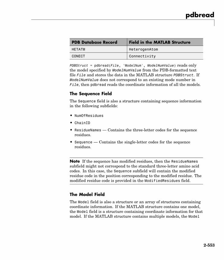
pdbread
PDB Database Record Field in the MATLAB Structure
HETATM HeterogenAtom
CONECT Connectivity
PDBStruct = pdbread(File, 'ModelNum', ModelNumValue) reads onlythe model specified by ModelNumValue from the PDB-formatted textfile File and stores the data in the MATLAB structure PDBStruct. IfModelNumValue does not correspond to an existing mode number inFile, then pdbread reads the coordinate information of all the models.
The Sequence Field
The Sequence field is also a structure containing sequence informationin the following subfields:
• NumOfResidues
• ChainID
• ResidueNames — Contains the three-letter codes for the sequenceresidues.
• Sequence — Contains the single-letter codes for the sequenceresidues.
Note If the sequence has modified residues, then the ResidueNamessubfield might not correspond to the standard three-letter amino acidcodes. In this case, the Sequence subfield will contain the modifiedresidue code in the position corresponding to the modified residue. Themodified residue code is provided in the ModifiedResidues field.
The Model Field
The Model field is also a structure or an array of structures containingcoordinate information. If the MATLAB structure contains one model,the Model field is a structure containing coordinate information for thatmodel. If the MATLAB structure contains multiple models, the Model
2-553

pdbread
field is an array of structures containing coordinate information foreach model. The Model field contains the following subfields:
• Atom
• AtomSD
• AnisotropicTemp
• AnisotropicTempSD
• Terminal
• HeterogenAtom
The Atom Field
The Atom field is also an array of structures containing the followingsubfields:
• AtomSerNo
• AtomName
• altLoc
• resName
• chainID
• resSeq
• iCode
• X
• Y
• Z
• occupancy
• tempFactor
• segID
• element
2-554
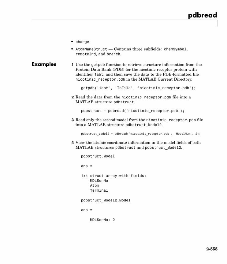
pdbread
• charge
• AtomNameStruct — Contains three subfields: chemSymbol,remoteInd, and branch.
Examples 1 Use the getpdb function to retrieve structure information from theProtein Data Bank (PDB) for the nicotinic receptor protein withidentifier 1abt, and then save the data to the PDB-formatted filenicotinic_receptor.pdb in the MATLAB Current Directory.
getpdb('1abt', 'ToFile', 'nicotinic_receptor.pdb');
2 Read the data from the nicotinic_receptor.pdb file into aMATLAB structure pdbstruct.
pdbstruct = pdbread('nicotinic_receptor.pdb');
3 Read only the second model from the nicotinic_receptor.pdb fileinto a MATLAB structure pdbstruct_Model2.
pdbstruct_Model2 = pdbread('nicotinic_receptor.pdb', 'ModelNum', 2);
4 View the atomic coordinate information in the model fields of bothMATLAB structures pdbstruct and pdbstruct_Model2.
pdbstruct.Model
ans =
1x4 struct array with fields:MDLSerNoAtomTerminal
pdbstruct_Model2.Model
ans =
MDLSerNo: 2
2-555
pdbread
Atom: [1x1205 struct]Terminal: [1x2 struct]
5 Read the data from an URL into a MATLAB structure,gfl_pdbstruct.
gfl_pdbstruct = pdbread('http://www.rcsb.org/pdb/files/1gfl.pdb');
See Also Bioinformatics Toolbox functions: genpeptread, getpdb, molviewer,pdbdistplot, pdbwrite
2-556
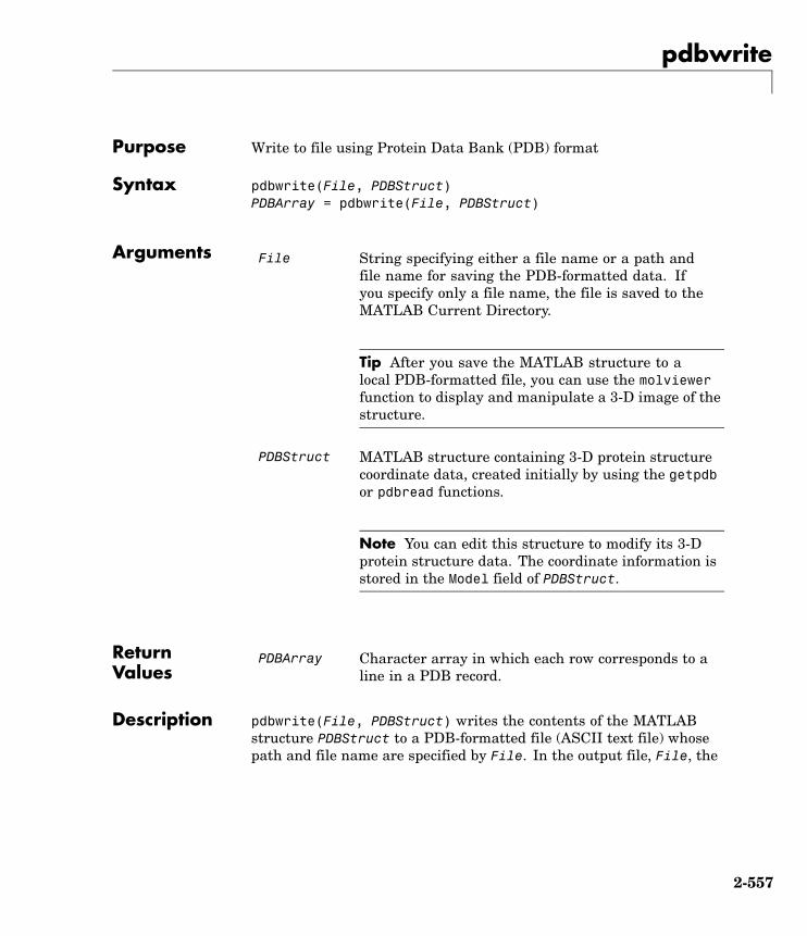
pdbwrite
Purpose Write to file using Protein Data Bank (PDB) format
Syntax pdbwrite(File, PDBStruct)PDBArray = pdbwrite(File, PDBStruct)
Arguments File String specifying either a file name or a path andfile name for saving the PDB-formatted data. Ifyou specify only a file name, the file is saved to theMATLAB Current Directory.
Tip After you save the MATLAB structure to alocal PDB-formatted file, you can use the molviewerfunction to display and manipulate a 3-D image of thestructure.
PDBStruct MATLAB structure containing 3-D protein structurecoordinate data, created initially by using the getpdbor pdbread functions.
Note You can edit this structure to modify its 3-Dprotein structure data. The coordinate information isstored in the Model field of PDBStruct.
ReturnValues
PDBArray Character array in which each row corresponds to aline in a PDB record.
Description pdbwrite(File, PDBStruct) writes the contents of the MATLABstructure PDBStruct to a PDB-formatted file (ASCII text file) whosepath and file name are specified by File. In the output file, File, the
2-557

pdbwrite
atom serial numbers are preserved. The atomic coordinate records areordered according to their atom serial numbers.
Tip After you save the MATLAB structure to a local PDB-formattedfile, you can use the molviewer function to display and manipulate a3-D image of the structure.
PDBArray = pdbwrite(File, PDBStruct) saves the formattedPDB record, converted from the contents of the MATLAB structurePDBStruct, to PDBArray, a character array in which each rowcorresponds to a line in a PDB record.
Note You can edit PDBStruct to modify its 3-D protein structure data.The coordinate information is stored in the Model field of PDBStruct.
Examples 1 Use the getpdb function to retrieve structure information fromthe Protein Data Bank (PDB) for the green fluorescent proteinwith identifier 1GFL , and store the data in the MATLAB structuregflstruct.
gflstruct = getpdb('1GFL');
2 Find the x-coordinate of the first atom.
gflstruct.Model.Atom(1).X
ans =
-14.0930
3 Edit the x-coordinate of the first atom.
gflstruct.Model.Atom(1).X = -18;
2-558
pdbwrite
Note Do not add or remove any Atom fields, because the pdbwritefunction does not allow the number of elements in the structure tochange.
4 Write the modified MATLAB structure gflstruct to a newPDB-formatted file modified_gfl.pdb in the Work directory on yourC drive.
pdbwrite('c:\work\modified_gfl.pdb', gflstruct);
5 Use the pdbread function to read the modified PDB file into aMATLAB structure, then confirm that the x-coordinate of the firstatom has changed.
modified_gflstruct = pdbread('c:\work\modified_gfl.pdb')modified_gflstruct.Model.Atom(1).X
ans =
-18
See Also Bioinformatics Toolbox functions: getpdb, molviewer, pdbread
2-559

pfamhmmread
Purpose Read data from PFAM-HMM file
Syntax Data = pfamhmmread('File')
Arguments File PFAM-HMM formatted file. Enter a file name, a path and filename, or a URL pointing to a file. File can also be a MATLABcharacter array that contains the text of a PFAM-HMM file.
Description pfamhmmread reads data from a PFAM-HMM formatted file (file savedwith the function gethmmprof) and creates a MATLAB structure.
Data = pfamhmmread('File') reads from File a Hidden Markov Modeldescribed by the PFAM format, and converts it to the MATLABstructure Data, containing fields corresponding to annotations andparameters of the model. For more information about the modelstructure format, see hmmprofstruct. File can also be a URL or aMATLAB cell array that contains the text of a PFAM formatted file.
pfamhmmread is based on the HMMER 2.0 file formats.
Examples pfamhmmread('pf00002.ls')
site='http://www.sanger.ac.uk/';pfamhmmread([site 'cgi-bin/Pfam/download_hmm.pl?mode=ls&id=7tm_2'])
See Also Bioinformatics Toolbox functions: gethmmalignment, gethmmprof,hmmprofalign, hmmprofstruct, showhmmprof
2-560
phytree
Purpose Create phytree object
Syntax Tree = phytree(B)Tree = phytree(B, D)Tree = phytree(B, C)Tree = phytree(BC)Tree = phytree(..., N)Tree = phytree
ArgumentsB Numeric array of size [NUMBRANCHES X 2] in which every row
represents a branch of the tree. It contains two pointers to thebranch or leaf nodes, which are its children.
C Column vector with distances for every branch.
D Column vector with distances from every node to their parentbranch.
BC Combined matrix with pointers to branches or leaves, anddistances of branches.
N Cell array with the names of leaves and branches.
Description Tree = phytree(B) creates an ultrametric phylogenetic tree object. Inan ultrametric phylogenetic tree object, all leaves are the same distancefrom the root.
B is a numeric array of size [NUMBRANCHES X 2] in which every rowrepresents a branch of the tree and it contains two pointers to thebranch or leaf nodes, which are its children.
Leaf nodes are numbered from 1 to NUMLEAVES and branch nodes arenumbered from NUMLEAVES + 1 to NUMLEAVES + NUMBRANCHES. Notethat because only binary trees are allowed, NUMLEAVES = NUMBRANCHES+ 1.
Branches are defined in chronological order (for example, B(i,:) >NUMLEAVES + i). As a consequence, the first row can only have pointersto leaves, and the last row must represent the root branch. Parent-child
2-561
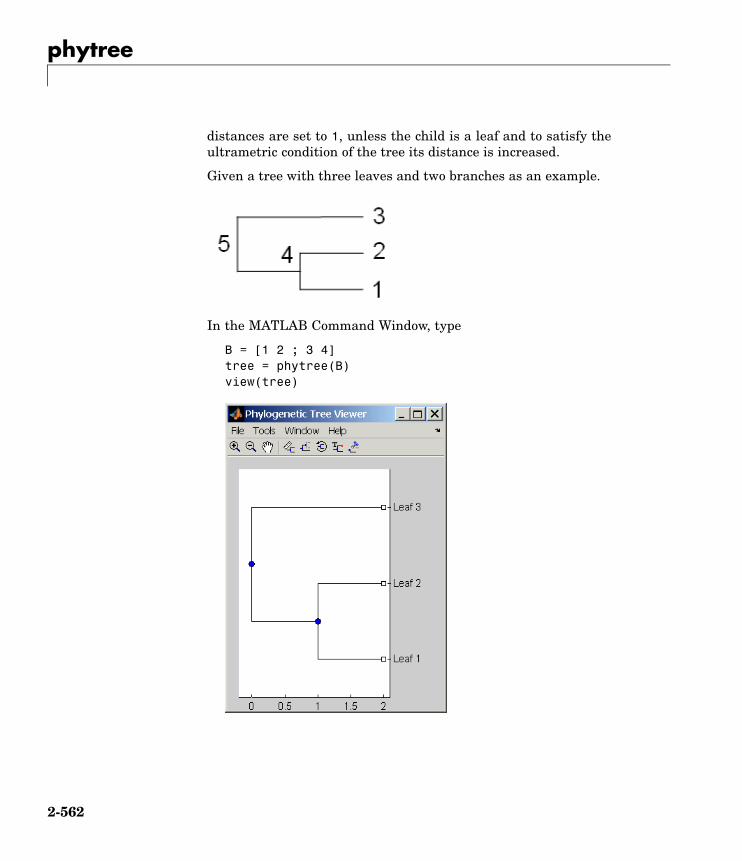
phytree
distances are set to 1, unless the child is a leaf and to satisfy theultrametric condition of the tree its distance is increased.
Given a tree with three leaves and two branches as an example.
In the MATLAB Command Window, type
B = [1 2 ; 3 4]tree = phytree(B)view(tree)
2-562
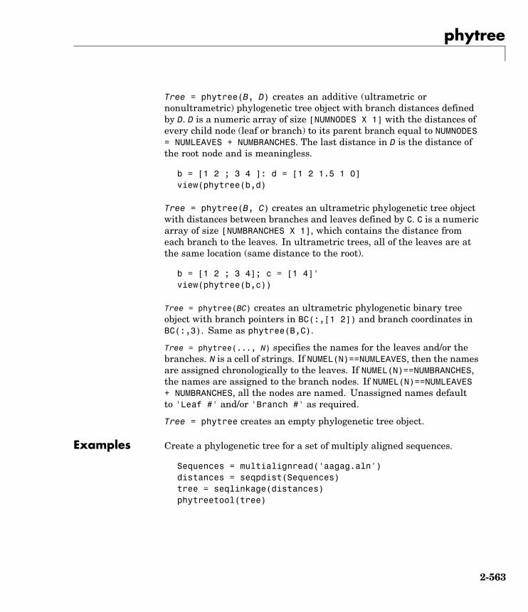
phytree
Tree = phytree(B, D) creates an additive (ultrametric ornonultrametric) phylogenetic tree object with branch distances definedby D. D is a numeric array of size [NUMNODES X 1] with the distances ofevery child node (leaf or branch) to its parent branch equal to NUMNODES= NUMLEAVES + NUMBRANCHES. The last distance in D is the distance ofthe root node and is meaningless.
b = [1 2 ; 3 4 ]: d = [1 2 1.5 1 0]view(phytree(b,d)
Tree = phytree(B, C) creates an ultrametric phylogenetic tree objectwith distances between branches and leaves defined by C. C is a numericarray of size [NUMBRANCHES X 1], which contains the distance fromeach branch to the leaves. In ultrametric trees, all of the leaves are atthe same location (same distance to the root).
b = [1 2 ; 3 4]; c = [1 4]'view(phytree(b,c))
Tree = phytree(BC) creates an ultrametric phylogenetic binary treeobject with branch pointers in BC(:,[1 2]) and branch coordinates inBC(:,3). Same as phytree(B,C).
Tree = phytree(..., N) specifies the names for the leaves and/or thebranches. N is a cell of strings. If NUMEL(N)==NUMLEAVES, then the namesare assigned chronologically to the leaves. If NUMEL(N)==NUMBRANCHES,the names are assigned to the branch nodes. If NUMEL(N)==NUMLEAVES+ NUMBRANCHES, all the nodes are named. Unassigned names defaultto 'Leaf #' and/or 'Branch #' as required.
Tree = phytree creates an empty phylogenetic tree object.
Examples Create a phylogenetic tree for a set of multiply aligned sequences.
Sequences = multialignread('aagag.aln')distances = seqpdist(Sequences)tree = seqlinkage(distances)phytreetool(tree)
2-563

phytree
See Also Bioinformatics Toolbox functions: phytreeread, phytreetool,phytreewrite, seqlinkage, seqneighjoin, seqpdist
Bioinformatics Toolbox object: phytree object
Bioinformatics Toolbox methods of phytree object: get, getbyname,getcanonical, getmatrix, getnewickstr, pdist, plot, prune, reroot,select, subtree, view, weights
2-564
phytreeread
Purpose Read phylogenetic tree file
Syntax Tree = phytreeread(File)
ArgumentsFile Newick-formatted tree files (ASCII text file). Enter a file
name, a path and file name, or a URL pointing to a file. Filecan also be a MATLAB character array that contains thetext for a file.
Tree phytree object created with the function phytree.
Description Tree = phytreeread(File) reads a Newick formatted tree file andreturns a phytree object in the MATLAB workspace with data fromthe file.
The NEWICK tree format can be found at
http://evolution.genetics.washington.edu/phylip/newicktree.html
Note This implementation only allows binary trees. Non-binary treesare translated into a binary tree with extra branches of length 0.
Examples tr = phytreeread('pf00002.tree')
See Also Bioinformatics Toolbox functions: phytree (object constructor),gethmmtree, phytreetool, phytreewrite
2-565
phytreetool
Purpose View, edit, and explore phylogenetic tree data
Syntax phytreetool(Tree)phytreetool(File)
ArgumentsTree Phytree object created with the functions phytree or
phytreeread.
File Newick or ClustalW tree formatted file (ASCII text file) withphylogenetic tree data. Enter a file name, a path and filename, or a URL pointing to a file. File can also be a MATLABcharacter array that contains the text for a Newick file.
Description phytreetool is an interactive GUI that allows you to view, edit, andexplore phylogenetic tree data. This GUI allows branch pruning,reordering, renaming, and distance exploring. It can also open or saveNewick formatted files.
phytreetool(Tree) loads data from a phytree object in the MATLABworkspace into the GUI.
phytreetool(File) loads data from a Newick formatted file into theGUI.
Examples tr= phytreeread('pf00002.tree')phytreetool(tr)
2-566
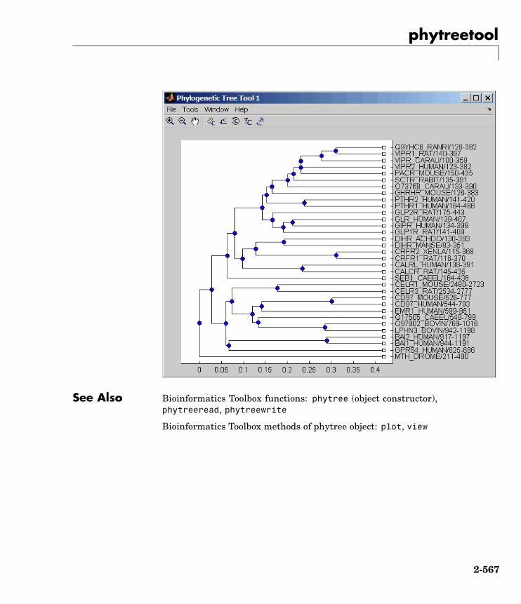
phytreetool
See Also Bioinformatics Toolbox functions: phytree (object constructor),phytreeread, phytreewrite
Bioinformatics Toolbox methods of phytree object: plot, view
2-567

phytreewrite
Purpose Write phylogenetic tree object to Newick-formatted file
Syntax phytreewrite('File', Tree)phytreewrite(Tree)
ArgumentsFile Newick-formatted file. Enter either a file name or a
path and file name supported by your operating system(ASCII text file).
Tree Phylogenetic tree object, either created with phytree(object constructor function) or imported using thephytreeread function.
Description phytreewrite('File', Tree) copies the contents of a phytree objectfrom the MATLAB workspace to a file. Data in the file uses the Newickformat for describing trees.
The Newick tree format can be found at
http://evolution.genetics.washington.edu/phylip/newicktree.html
phytreewrite(Tree) opens the Save Phylogenetic Tree As dialog box foryou to enter or select a file name.
Examples Read tree data from a Newick-formatted file.
tr = phytreeread('pf00002.tree')
Remove all the mouse proteins
ind = getbyname(tr,'mouse');tr = prune(tr,ind);
2-568
phytreewrite
view(tr)
Write pruned tree data to a file.
phytreewrite('newtree.tree', tr)
See Also Bioinformatics Toolbox functions: phytree (object constructor),phytreeread, phytreetool, seqlinkage
Bioinformatics Toolbox object: phytree object
Bioinformatics Toolbox methods of phytree object: getnewickstr
2-569
probelibraryinfo
Purpose Probe set library information for probe results
Syntax ProbeInfo = probelibraryinfo(CELStruct, CDFStruct)
Description ProbeInfo = probelibraryinfo(CELStruct, CDFStruct)creates atable of information linking the probe data in a CEL file structure withprobe set information from a CDF file structure.
ProbeInfo is a matrix with three columns and the same number ofrows as the probes field of the CELStruct. The first column is the probeset ID number to which the probe belongs. (Probes that do not belongto a probe set in the CDF library file have probe set ID equal to 0.)The second column contains the probe pair number. The third columnindicates if the probe is a perfect match (1) or mismatch (-1) probe.
Note Affymetrix probe pair indexing is 0 based while MATLABindexing is 1 based. The output from probelibraryinfo is 1 based.
Examples 1 Get the file Drosophila-121502.cel from
http://www.affymetrix.com/support/technical/sample_data/demo_data.affx
2 Read the data into MATLAB.
CELStruct = affyread('Drosophila-121502.cel');CDFStruct = affyread('D:\Affymetrix\LibFiles\...
DrosGenome1\DrosGenome1.CDF');
3 Extract probe set library information.
ProbeInfo = probelibraryinfo(CELStruct, CDFStruct);
4 Find out probe set to which the 1104th probe belongs.
CDFStruct.ProbeSets(ProbeInfo(1104,1)).Name
2-570

probelibraryinfo
See Also Bioinformatics Toolbox functions: affyread, celintensityread,probesetlink, probesetlookup, probesetvalues
2-571

probesetlink
Purpose Link to NetAffx Web site
Syntax probesetlink(AFFYStruct, ID)URL = probesetlink(AFFYStruct, ID)probesetlink(..., 'PropertyName', PropertyValue,...)probesetlink(..., 'Source', SourceValue),probesetlink(..., 'Browser', BrowserValue)probesetlink(..., 'NoDisplay', NoDisplayValue)
Description probesetlink(AFFYStruct, ID) displays information from theNetAffx Web site about a probe set (ID) from the CHP or CDF structure(AFFYStruct). ID can be the index of the probe set or the probe setname.
URL = probesetlink(AFFYStruct, ID) returns the URL for theinformation.
probesetlink(..., 'PropertyName', PropertyValue,...) definesoptional properties using property name/value pairs.
probesetlink(..., 'Source', SourceValue), when SourceValue istrue, links to the data source (e.g., GenBank, Flybase) for the probe set.
probesetlink(..., 'Browser', BrowserValue), when BrowserValueis true, displays the information in the system Web browser.
probesetlink(..., 'NoDisplay', NoDisplayValue), whenNoDisplayValue is true, returns the URL but does not open a browser.
Note NetAffx Web site requires you to register and provide a username and password.
Examples 1 Get the file Drosophila-121502.chp from
http://www.affymetrix.com/support/technical/sample_data/demo_data.affx
2 Read the data into MATLAB.
2-572
probesetlink
chpStruct = affyread('Drosophila-121502.chp',...'D:\Affymetrix\LibFiles\DrosGenome1')
3 Display information from the NetAffx Web site.
probesetlink(chpStruct,'AFFX-YEL018w/_at');
See Also Bioinformatics Toolbox functions: affyread, celintensityread,probelibraryinfo, probesetlookup, probesetplot, probesetvalues
2-573

probesetlookup
Purpose Gene name for probe set
Syntax probesetlookup(AFFYStruct, ID)probesetlookup(AFFYStruct, Name)[Name, NDX, Description, Source,
SourceURL] = probesetlookup(...)
Description probesetlookup(AFFYStruct, ID) returns the gene name for a probeset ID from a CHP or CDF structure (AFFYStruct).
probesetlookup(AFFYStruct, Name) returns the probe set ID for agene name (Name) from a CHP or CDF structure (AFFYStruct).
[Name, NDX, Description, Source, SourceURL] =probesetlookup(...) returns the name, index into the CHP or CDFstruct, description, source, and source URL and for the probe set.
Note This function requires that you have the GIN file associated withthe chip type that you are using in your Affymetrix library directory.
Examples 1 Get the file Drosophila-121502.chp from
http://www.affymetrix.com/support/technical/sample_data/demo_data.affx
2 Read the data into MATLAB.
chpStruct = affyread('Drosophila-121502.chp',...'D:\Affymetrix\LibFiles\DrosGenome1')
3 Get the gene name.
probesetlookup(chpStruct,'AFFX-YEL018w/_at')
See Also Bioinformatics Toolbox functions: affyread, celintensityread,probelibraryinfo, probesetlink, probesetplot, probesetvalues,rmabackadj
2-574
probesetplot
Purpose Plot values for Affymetrix CHP file probe set
Syntax probesetplot(CHPStruct, ID, 'PropertyName', PropertyValue)probesetplot(..., 'GeneName', GeneNameValue)probesetplot(..., 'Field', FieldValue)probesetplot(..., 'ShowStats',ShowStatsValue)
Description probesetplot(CHPStruct, ID, 'PropertyName', PropertyValue)plots the PM and MM intensity values for probe set ID. CHPStruct is astructure created from an Affymetrix CHP file. ID can be the index ofthe probe set or the probe set name. Note: the probe set numbers fora CHP file use 0 based indexing while MATLAB uses 1 based indexing.CHPStruct.ProbeSets(1) has ProbeSetNumber 0.
probesetplot(..., 'GeneName', GeneNameValue) when GeneName istrue, uses the gene name, rather than the probeset name for the title.
probesetplot(..., 'Field', FieldValue) shows the data for a field(FieldValue). Valid fieldnames are: Background, Intensity, StdDev,Pixels, and Outlier.
probesetplot(..., 'ShowStats',ShowStatsValue) when ShowStatsis true, adds mean and standard deviation lines to the plot.
Examples 1 Get the file Drosophila-121502.chp from
http://www.affymetrix.com/support/technical/sample_data/demo_data.affx
2 Read the data into MATLAB.
chpStruct = affyread('Drosophila-121502.chp',...'D:\Affymetrix\LibFiles\DrosGenome1')
3 Plots PM and MM intensity values.
probesetplot(chpStruct,'AFFX-YEL018w/_at','showstats',true);
See Also Bioinformatics Toolbox functions: affyread, celintensityread,probesetlink, probesetlookup
2-575

probesetvalues
Purpose Probe set values from probe results
Syntax PSValues = probesetvalues(CELStruct,CDFStruct,PS)
Description PSValues = probesetvalues(CELStruct,CDFStruct,PS) creates atable of values for a probe set (PS) from the probe data in a CEL filestructure (CELStruct). PS is a probe set index or probe set name fromthe CDF library file structure (CDFStruct). PSValues is a matrix with18 columns and one row for each probe pair in the probe set. Thecolumns correspond to the fields in a CHP probe set data structure:
'ProbeSetNumber''ProbePairNumber''UseProbePair''Background''PMPosX''PMPosY''PMIntensity''PMStdDev''PMPixels''PMOutlier''PMMasked''MMPosX''MMPosY''MMIntensity''MMStdDev''MMPixels''MMOutlier''MMMasked'
There are some minor differences between the output of this functionand the data in a CHP file. The PM and MM Intensity values in the CHPfile are normalized by the Affymetrix software. This function returnsthe raw intensity values. The 'UseProbePair' and 'Background' fieldsare only returned by this function for compatibility with the CHP probeset data structure and are always set to zero.
2-576

probesetvalues
Examples 1 Get the file Drosophila-121502.cel from
http://www.affymetrix.com/support/technical/sample_data/demo_data.affx
2 Read the data into MATLAB.
celStruct = affyread('Drosophila-121502.cel');cdfStruct = affyread('D:\Affymetrix\LibFiles\DrosGenome1\...
DrosGenome1.CDF');
3 Get the values for probe set 147439_at.
psvals = probesetvalues(celStruct,cdfStruct,'147439_at')
See Also Bioinformatics Toolbox functions: affyread, celintensityread,probelibraryinfo, probesetlink, probesetlookup, rmabackadj
2-577

profalign
Purpose Align two profiles using Needleman-Wunsch global alignment
Syntax Prof = profalign(Prof1, Prof2)[Prof, H1, H2] = profalign(Prof1, Prof2)profalign(..., 'PropertyName', PropertyValue,...)profalign(..., 'ScoringMatrix', ScoringMatrixValue)profalign(..., 'GapOpen', {G1Value, G2Value})profalign(..., 'ExtendGap', {E1Value, E2Value})profalign(..., 'ExistingGapAdjust', ExistingGapAdjustValue)profalign(..., 'TerminalGapAdjust', TerminalGapAdjustValue)profalign(..., 'ShowScore', ShowScoreValue)
Description Prof = profalign(Prof1, Prof2) returns a new profile (Prof) for theoptimal global alignment of two profiles (Prof1, Prof2). The profiles(Prof1, Prof2) are numeric arrays of size [(4 or 5 or 20 or 21) xProfile Length] with counts or weighted profiles. Weighted profilesare used to down-weight similar sequences and up-weight divergentsequences. The output profile is a numeric matrix of size [(5 or 21)x New Profile Length] where the last row represents gaps. Originalgaps in the input profiles are preserved. The output profile is the resultof adding the aligned columns of the input profiles.
[Prof, H1, H2] = profalign(Prof1, Prof2) returns pointers thatindicate how to rearrange the columns of the original profiles into thenew profile.
profalign(..., 'PropertyName', PropertyValue,...) definesoptional properties using property name/value pairs.
profalign(..., 'ScoringMatrix', ScoringMatrixValue) definesthe scoring matrix (ScoringMatrixValue) to be used for the alignment.The default is 'BLOSUM50' for amino acids or 'NUC44' for nucleotidesequences.
profalign(..., 'GapOpen', {G1Value, G2Value}) sets the penaltiesfor opening a gap in the first and second profiles respectively. G1Valueand G2Value can be either scalars or vectors. When using a vector, thenumber of elements is one more than the length of the input profile.Every element indicates the position specific penalty for opening a gap
2-578
profalign
between two consecutive symbols in the sequence. The first and the lastelements are the gap penalties used at the ends of the sequence. Thedefault gap open penalties are {10,10}.
profalign(..., 'ExtendGap', {E1Value, E2Value}) sets thepenalties for extending a gap in the first and second profile respectively.E1Value and E2Value can be either scalars or vectors. When usinga vector, the number of elements is one more than the length of theinput profile. Every element indicates the position specific penalty forextending a gap between two consecutive symbols in the sequence. Thefirst and the last elements are the gap penalties used at the ends of thesequence. If ExtendGap is not specified, then extensions to gaps arescored with the same value as GapOpen.
profalign(..., 'ExistingGapAdjust', ExistingGapAdjustValue),if ExistingGapAdjustValue is false, turns off the automaticadjustment based on existing gaps of the position-specific penaltiesfor opening a gap. When ExistingGapAdjustValue is true, for everyprofile position, profalign proportionally lowers the penalty foropening a gap toward the penalty of extending a gap based on theproportion of gaps found in the contiguous symbols and on the weightof the input profile.
profalign(..., 'TerminalGapAdjust', TerminalGapAdjustValue),when TerminalGapAdjustValue is true, adjusts the penalty foropening a gap at the ends of the sequence to be equal to the penalty forextending a gap. Default is false.
profalign(..., 'ShowScore', ShowScoreValue), whenShowScoreValue is true, displays the scoring space and the winningpath.
Examples 1 Read in sequences and create profiles.
ma1 = ['RGTANCDMQDA';'RGTAHCDMQDA';'RRRAPCDL-DA'];ma2 = ['RGTHCDLADAT';'RGTACDMADAA'];p1 = seqprofile(ma1,'gaps','all','counts',true);p2 = seqprofile(ma2,'counts',true);
2-579
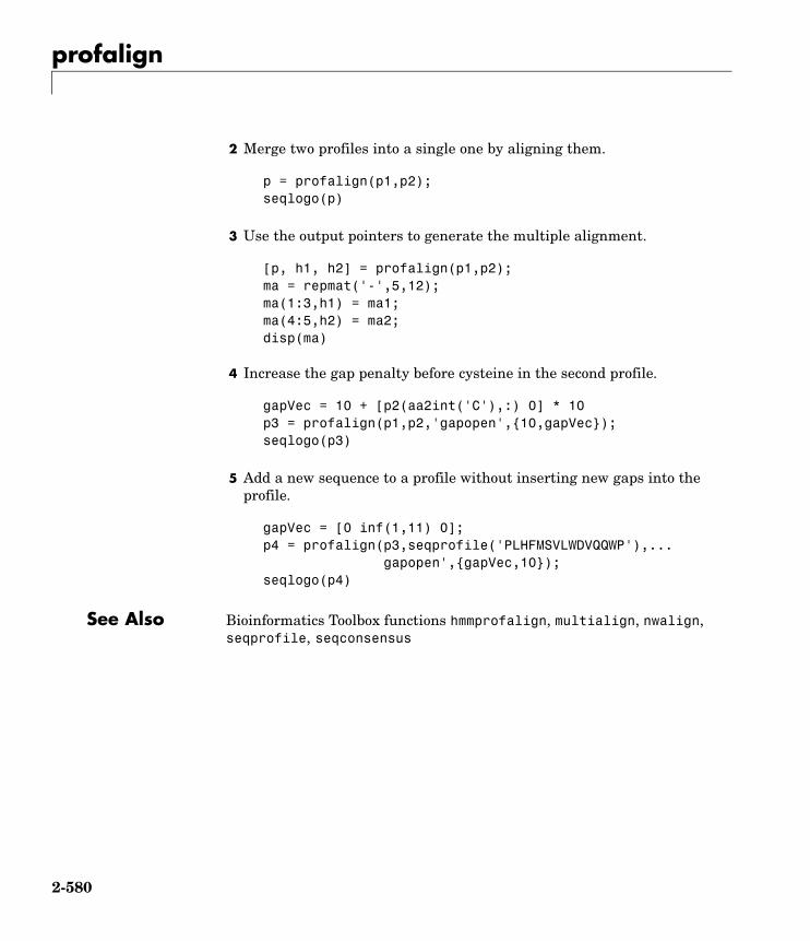
profalign
2 Merge two profiles into a single one by aligning them.
p = profalign(p1,p2);seqlogo(p)
3 Use the output pointers to generate the multiple alignment.
[p, h1, h2] = profalign(p1,p2);ma = repmat('-',5,12);ma(1:3,h1) = ma1;ma(4:5,h2) = ma2;disp(ma)
4 Increase the gap penalty before cysteine in the second profile.
gapVec = 10 + [p2(aa2int('C'),:) 0] * 10p3 = profalign(p1,p2,'gapopen',{10,gapVec});seqlogo(p3)
5 Add a new sequence to a profile without inserting new gaps into theprofile.
gapVec = [0 inf(1,11) 0];p4 = profalign(p3,seqprofile('PLHFMSVLWDVQQWP'),...
gapopen',{gapVec,10});seqlogo(p4)
See Also Bioinformatics Toolbox functions hmmprofalign, multialign, nwalign,seqprofile, seqconsensus
2-580

proteinplot
Purpose Characteristics for amino acid sequences
Syntax proteinplot (SeqAA)
ArgumentsSeqAA Amino acid sequence or a structure with a field Sequence
containing an amino acid sequence.
Description proteinplot (SeqAA) loads an amino acid sequence into the protein plotGUI. proteinplot is a tool for analyzing a single amino acid sequence.You can use the results from proteinplot to compare the propertiesof several amino acid sequences. It displays smoothed line plots ofvarious properties such as the hydrophobicity of the amino acids inthe sequence.
Importing Sequences into proteinplot
1 In the MATLAB Command Window, type
proteinplot(Seq_AA)
The proteinplot interface opens and the sequence Seq_AA is shownin the Sequence text box.
2 Alternatively, type or paste an amino acid sequence into theSequence text box.
You can import a sequence with the Import dialog box:
1 Click the Import Sequence button. The Import dialog box opens.
2 From the Import From list, select a variable in the MATLABworkspace, ASCII text file, FASTA formatted file, GenPept formattedfile, or accession number in the GenPept database.
2-581
proteinplot
Information About the Properties
You can also access information about the properties from the Helpmenu.
1 From the Help menu, click References. The Help Browser openswith a list of properties and references.
2 Scroll down to locate the property you are interested in studying.
Working with Properties
When you click on a property a smoothed plot of the property valuesalong the sequence will be displayed. Multiple properties can beselected from the list by holding down Shift or Ctrl while selectingproperties. When two properties are selected, the plots are displayedusing a PLOTYY-style layout, with one y-axis on the left and one onthe right. For all other selections, a single y-axis is displayed. Whendisplaying one or two properties, the y values displayed are the actualproperty values. When three or more properties are displayed, thevalues are normalized to the range 0-1.
You can add your own property values by clicking on the Add buttonnext to the property list. This will open up a dialog that allows you tospecify the values for each of the amino acids. The Display Text boxallows you to specify the text that will be displayed in the selection boxon the main proteinplot window. You can also save the property valuesto an m-file for future use by typing a file name into the Filename box.
The Terminal Selection boxes allow you to choose to plot only part ofthe sequence. By default all of the sequence is plotted. The defaultsmoothing method is an unweighted linear moving average witha window length of five residues. You can change this using the"Configuration Values" dialog from the Edit menu. The dialog allowsyou to select the window length from 5 to 29 residues. You can modifythe shape of the smoothing window by changing the edge weightingfactor. And you can choose the smoothing function to be a linear movingaverage, an exponential moving average or a linear Lowess smoothing.
2-582
proteinplot
The File menu allows you to Import a sequence, save the plot that youhave created to a FIG file, you can export the data values in the figureto a workspace variable or to a MAT file, you can export the figure to anormal figure window for customizing, and you can print the figure.
The Edit menu allows you to create a new property, to reset the propertyvalues to the default values, and to modify the smoothing parameterswith the Configuration Values menu item.
The View menu allows you to turn the toolbar on and off, and to adda legend to the plot.
The Tools menu allows you to zoom in and zoom out of the plot, to viewData Statistics such as mean, minimum and maximum values of theplot, and to normalize the values of the plot from 0 to 1.
The Help menu allows you to view this document and to see thereferences for the sequence properties built into proteinplot
See Also Bioinformatics Toolbox functions: aacount, atomiccomp, molviewer,molweight, pdbdistplot, seqtool
MATLAB function: plotyy
2-583

proteinpropplot
Purpose Plot properties of amino acid sequence
Syntax proteinpropplot (SeqAA)proteinpropplot(SeqAA, ...'PropertyTitle',PropertyTitleValue, ...)proteinpropplot(SeqAA, ...'Startat', StartatValue, ...)proteinpropplot(SeqAA, ...'Endat', EndatValue, ...)proteinpropplot(SeqAA, ...'Smoothing', SmoothingValue, ...)proteinpropplot(SeqAA, ...'EdgeWeight',EdgeWeightValue, ...)proteinpropplot(SeqAA, ...'WindowLength',WindowLengthValue,
...)
2-584

proteinpropplot
ArgumentsSeqAA Amino acid sequence. Enter any of the
following:• Character string of letters representing an
amino acid
• Vector of integers representing an aminoacid, such as returned by aa2int
• Structure containing a Sequence field thatcontains an amino acid sequence, such asreturned by getembl, getgenpept, or getpdb
PropertyTitleValue String that specifies the property toplot. Default is Hydrophobicity (Kyte& Doolittle). To display a list ofproperties to plot, enter a empty string forPropertyTitleValue. For example, type:
proteinpropplot(sequence, 'propertytitle', '')
Tip To access references for the properties,view the proteinpropplot m-file.
StartatValue Integer that specifies the starting point for theplot from the N-terminal end of the amino acidsequence SeqAA. Default is 1.
EndatValue Integer that specifies the ending point for theplot from the N-terminal end of the amino acidsequence SeqAA. Default is length(SeqAA).
SmoothingValue String the specifies the smoothing method.Choices are:• linear (default)
• exponential
• lowess
2-585
proteinpropplot
EdgeWeightValue Value that specifies the edge weight used forlinear and exponential smoothing methods.Decreasing this value emphasizes peaks in theplot. Choices are any value ≥0 and ≤1. Defaultis 1.
WindowLengthValue Integer that specifies the window length for thesmoothing method. Increasing this value givesa smoother plot that shows less detail. Defaultis 11.
Description proteinpropplot (SeqAA) displays a plot of the hydrophobicity (Kyteand Doolittle, 1982) of the residues in sequence SeqAA.
proteinpropplot(SeqAA, ...'PropertyName',PropertyValue, ...) calls proteinpropplot with optional propertiesthat use property name/property value pairs. You can specify one ormore properties in any order. Each PropertyName must be enclosedin single quotation marks and is case insensitive. These propertyname/property value pairs are as follows:
proteinpropplot(SeqAA, ...'PropertyTitle',PropertyTitleValue, ...) specifies a property to plot forthe amino acid sequence SeqAA. Default is Hydrophobicity (Kyte &Doolittle). To display a list of possible properties to plot, enter anempty string for PropertyTitleValue. For example, type:
proteinpropplot(sequence, 'propertytitle', '')
Tip To access references for the properties, view the proteinpropplotm-file.
proteinpropplot(SeqAA, ...'Startat', StartatValue, ...)specifies the starting point for the plot from the N-terminal end of theamino acid sequence SeqAA. Default is 1.
2-586

proteinpropplot
proteinpropplot(SeqAA, ...'Endat', EndatValue, ...) specifiesthe ending point for the plot from the N-terminal end of the amino acidsequence SeqAA. Default is length(SeqAA).
proteinpropplot(SeqAA, ...'Smoothing', SmoothingValue, ...)specifies the smoothing method. Choices are:
• linear (default)
• exponential
• lowess
proteinpropplot(SeqAA, ...'EdgeWeight',EdgeWeightValue, ...) specifies the edge weight used for linear andexponential smoothing methods. Decreasing this value emphasizespeaks in the plot. Choices are any value ≥0 and ≤1. Default is 1.
proteinpropplot(SeqAA, ...'WindowLength',WindowLengthValue, ...) specifies the window length for thesmoothing method. Increasing this value gives a smoother plot thatshows less detail. Default is 11.
Examples Plotting Hydrophobicity
1 Use the getpdb function to retrieve a protein sequence.
prion = getpdb('1HJM', 'SEQUENCEONLY', true);
2 Plot the hydrophobicity (Kyte and Doolittle, 1982) of the residuesin the sequence.
proteinpropplot(prion)
2-587

proteinpropplot
Plotting Parallel Beta Strand
1 Use the getgenpept function to retrieve a protein sequence.
s = getgenpept('aad50640');
2 Plot the conformational preference for parallel beta strand for theresidues in the sequence.
proteinpropplot(s,'propertytitle','Parallel beta strand')
2-588
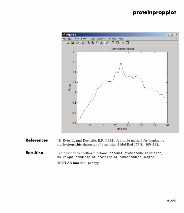
proteinpropplot
References [1] Kyte, J., and Doolittle, R.F. (1982). A simple method for displayingthe hydropathic character of a protein. J Mol Biol 157(1), 105–132.
See Also Bioinformatics Toolbox functions: aacount, atomiccomp, molviewer,molweight, pdbdistplot, proteinplot, ramachandran, seqtool
MATLAB function: plotyy
2-589
quantilenorm
Purpose Quantile normalization over multiple arrays
Syntax NormData = quantilenorm(Data)NormData = quantilenorm(...,'MEDIAN', true)NormData = quantilenorm(...,'DISPLAY', true)
Description NormData = quantilenorm(Data), where the columns of Datacorrespond to separate chips, normalizes the distributions of the valuesin each column.
Note If Data contains NaN values, then NormData will also containNaN values at the corresponding positions.
NormData = quantilenorm(...,'MEDIAN', true) takes the median ofthe ranked values instead of the mean.
NormData = quantilenorm(...,'DISPLAY', true) plots thedistributions of the columns and of the normalized data.
Examples load yeastdatanormYeastValues = quantilenorm(yeastvalues,'display',1);
See Also malowess, manorm, rmabackadj, rmasummary
2-590

ramachandran
Purpose Draw Ramachandran plot for Protein Data Bank (PDB) data
Syntax ramachandran('PDBid')ramachandran('File')ramachandran(PDBData)Angles = ramachandran(...)[Angles, Handle] = ramachandran(...)
ArgumentsPDBid Unique identifier for a protein structure record. Each
structure in the PDB is represented by a 4-characteralphanumeric identifier. For example, 4hhb is theidentification code for hemoglobin.
File Protein Data Bank (PDB) formatted file (ASCII textfile). Enter a file name, a path and file name, or a URLpointing to a file. File can also be a MATLAB characterarray that contains the text for a PDB file.
PDBData MATLAB structure with PDB formatted data.
Description ramachandran generates a plot of the torsion angle PHI (torsion anglebetween the 'C-N-CA-C' atoms) and the torsion angle PSI (torsionangle between the 'N-CA-C-N' atoms) of the protein sequence.
ramachandran('PDBid') generates the Ramachandran plot for theprotein with PDB code ID.
ramachandran('File') generates the Ramachandran plot for proteinstored in the PDB file File.
ramachandran(PDBData) generates the Ramachandran plot for theprotein stored in the structure PDBData, where PDBData is a MATLABstructure obtained by using pdbread or getpdb.
Angles = ramachandran(...) returns an array of the torsion anglesPHI, PSI, and OMEGA for the residue sequence.
[Angles, Handle] = ramachandran(...) returns a handle to the plot.
2-591
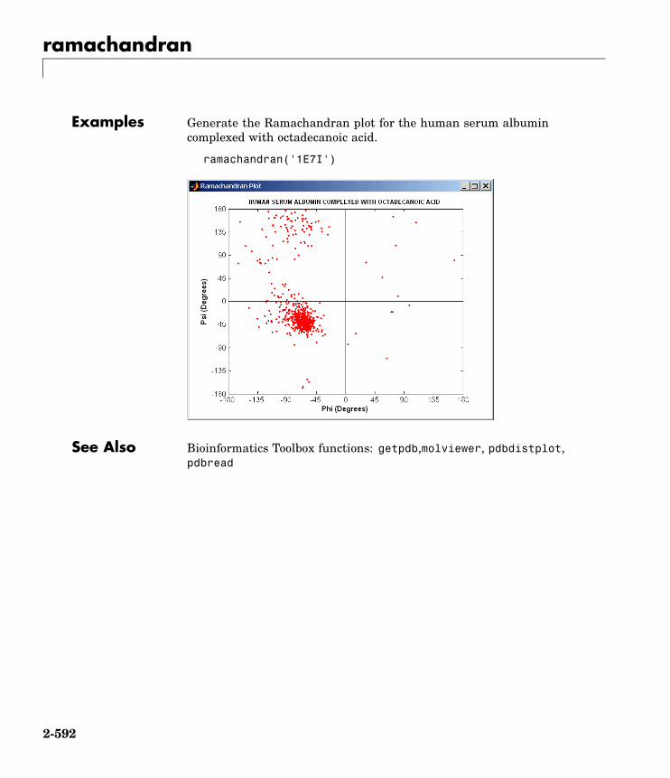
ramachandran
Examples Generate the Ramachandran plot for the human serum albumincomplexed with octadecanoic acid.
ramachandran('1E7I')
See Also Bioinformatics Toolbox functions: getpdb,molviewer, pdbdistplot,pdbread
2-592
randfeatures
Purpose Generate randomized subset of features
Syntax [IDX, Z] = randfeatures(X, Group, 'PropertyName',PropertyValue...)
randfeatures(..., 'Classifier', C)randfeatures(..., 'ClassOptions', CO)randfeatures(..., 'PerformanceThreshold', PT)randfeatures(..., 'ConfidenceThreshold', CT)randfeatures(..., 'SubsetSize', SS)randfeatures(..., 'PoolSize', PS)randfeatures(..., 'NumberOfIndices', N)randfeatures(..., 'CrossNorm', CN)randfeatures(..., 'Verbose', VerboseValue)
Description [IDX, Z] = randfeatures(X, Group, 'PropertyName',PropertyValue...) performs a randomized subset feature searchreinforced by classification. randfeatures randomly generates subsetsof features used to classify the samples. Every subset is evaluated withthe apparent error. Only the best subsets are kept, and they are joinedinto a single final pool. The cardinality for every feature in the poolgives the measurement of the significance.
X contains the training samples. Every column of X is an observedvector. Group contains the class labels. Group can be a numeric vector ora cell array of strings; numel(Group) must be the same as the numberof columns in X, and numel(unique(Group)) must be greater than orequal to 2. Z is the classification significance for every feature. IDXcontains the indices after sorting Z; i.e., the first one points to the mostsignificant feature.
randfeatures(..., 'Classifier', C) sets the classifier. Options are
'da' (default) Discriminant analysis'knn' K nearest neighbors
randfeatures(..., 'ClassOptions', CO)is a cell withextra options for the selected classifier. Defaults are
2-593
randfeatures
{5,'correlation','consensus'} for KNN and {'linear'} for DA. Seeknnclassify and classify for more information.
randfeatures(..., 'PerformanceThreshold', PT) sets the correctclassification threshold used to pick the subsets included in the finalpool. Default is 0.8 (80%).
randfeatures(..., 'ConfidenceThreshold', CT) uses the posteriorprobability of the discriminant analysis to invalidate classifiedsubvectors with low confidence. This option is only valid whenClassifier is 'da'. Using it has the same effect as using 'consensus'in KNN; i.e., it makes the selection of approved subsets very stringent.Default is 0.95.^(number of classes).
randfeatures(..., 'SubsetSize', SS) sets the number of featuresconsidered in every subset. Default is 20.
randfeatures(..., 'PoolSize', PS) sets the targeted number ofaccepted subsets for the final pool. Default is 1000.
randfeatures(..., 'NumberOfIndices', N) sets the number ofoutput indices in IDX. Default is the same as the number of features.
randfeatures(..., 'CrossNorm', CN) applies independentnormalization across the observations for every feature.Cross-normalization ensures comparability among different features,although it is not always necessary because the selected classifierproperties might already account for this. Options are
'none' (default) Intensities are not cross-normalized.'meanvar' x_new = (x - mean(x))/std(x)'softmax' x_new = (1+exp((mean(x)-x)/std(x)))^-1'minmax' x_new = (x - min(x))/(max(x)-min(x))
randfeatures(..., 'Verbose', VerboseValue), when Verbose istrue, turns off verbosity. Default is true.
Examples Find a reduced set of genes that is sufficient for classification of all thecancer types in the t-matrix NCI60 data set. Load sample data.
2-594
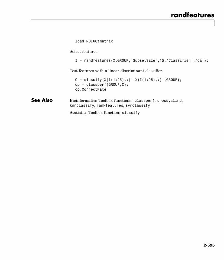
randfeatures
load NCI60tmatrix
Select features.
I = randfeatures(X,GROUP,'SubsetSize',15,'Classifier','da');
Test features with a linear discriminant classifier.
C = classify(X(I(1:25),:)',X(I(1:25),:)',GROUP);cp = classperf(GROUP,C);cp.CorrectRate
See Also Bioinformatics Toolbox functions: classperf, crossvalind,knnclassify, rankfeatures, svmclassify
Statistics Toolbox function: classify
2-595

randseq
Purpose Generate random sequence from finite alphabet
Syntax Seq = randseq(SeqLength)Seq = randseq(SeqLength, ...'Alphabet', AlphabetValue, ...)Seq = randseq(SeqLength, ...'Weights', WeightsValue, ...)Seq = randseq(SeqLength, ...'FromStructure',
FromStructureValue, ...)Seq = randseq(SeqLength, ...'Case', CaseValue, ...)Seq = randseq(SeqLength, ...'DataType', DataTypeValue, ...)
ArgumentsSeqLength Number of amino acids or nucleotides in
random sequence .
AlphabetValue Property to select the alphabet for thesequence. Enter 'dna'(default), 'rna', or'amino'.
WeightsValue Property to specify a weighted randomsequence.
FromStructureValue Property to specify a weighted randomsequence using output structures from thefunctions from basecount, dimercount,codoncount, or aacount.
CaseValue Property to select the case of letters in asequence whenAlphabet is 'char'. Valuesare'upper' (default) or 'lower'.
DataTypeValue Property to select the data type for asequence. Values are 'char'(default) forletter sequences, and 'uint8' or 'double'for numeric sequences.
Creates a sequence as an array of DataType.
Description Seq = randseq(SeqLength) creates a random sequence with a lengthspecified by SeqLength.
2-596
randseq
Seq = randseq(SeqLength, ...'PropertyName',PropertyValue, ...) calls randseq with optional propertiesthat use property name/property value pairs. You can specify one ormore properties in any order. Each PropertyName must be enclosed insingle quotes and is case insensitive. These property name/propertyvalue pairs are as follows:
Seq = randseq(SeqLength, ...'Alphabet', AlphabetValue, ...)generates a sequence from a specific alphabet.
Seq = randseq(SeqLength, ...'Weights', WeightsValue, ...)creates a weighted random sequence where the ith letter of thesequence alphabet is selected with weight W(i). The weight vector isusually a probability vector or a frequency count vector. Note that theith element of the nucleotide alphabet is given by int2nt(i), and theith element of the amino acid alphabet is given by int2aa(i).
Seq = randseq(SeqLength,...'FromStructure', FromStructureValue, ...) creates aweighted random sequence with weights given by the output structurefrom basecount, dimercount, codoncount, or aacount.
Seq = randseq(SeqLength, ...'Case', CaseValue, ...) specifiesthe case for a letter sequence.
Seq = randseq(SeqLength, ...'DataType', DataTypeValue, ...)specifies the data type for the sequence array.
Examples Generate a random DNA sequence.
randseq(20)
ans =TAGCTGGCCAAGCGAGCTTG
Generate a random RNA sequence.
randseq(20,'alphabet','rna')
ans =
2-597

randseq
GCUGCGGCGGUUGUAUCCUG
Generate a random protein sequence.
randseq(20,'alphabet','amino')
ans =DYKMCLYEFGMFGHFTGHKK
See Also Statistics Toolbox functions: hmmgenerate, randsample
MATLAB functions: rand, randperm
2-598

rankfeatures
Purpose Rank key features by class separability criteria
Syntax [IDX, Z] = rankfeatures(X, Group)[IDX, Z] = rankfeatures(X, Group, ...'Criterion',CriterionValue, ...)[IDX, Z] = rankfeatures(X, Group, ...'CCWeighting', ALPHA,
...)[IDX, Z] = rankfeatures(X, Group, ...'NWeighting',BETA, ...)[IDX, Z] = rankfeatures(X, Group, ...'NumberOfIndices', N,
...)[IDX, Z] = rankfeatures(X, Group, ...'CrossNorm', CN, ...)
Description [IDX, Z] = rankfeatures(X, Group) ranks the features in X usingan independent evaluation criterion for binary classification. X is amatrix where every column is an observed vector and the number ofrows corresponds to the original number of features. Group containsthe class labels.
IDX is the list of indices to the rows in X with the most significantfeatures. Z is the absolute value of the criterion used (see below).
Group can be a numeric vector or a cell array of strings; numel(Group)is the same as the number of columns in X, and numel(unique(Group))is equal to 2.
[IDX, Z] = rankfeatures(X, Group, ...'PropertyName',PropertyValue, ...) calls rankfeatures with optional propertiesthat use property name/property value pairs. You can specify one ormore properties in any order. Each PropertyName must be enclosedin single quotation marks and is case insensitive. These propertyname/property value pairs are as follows.
[IDX, Z] = rankfeatures(X, Group, ...'Criterion',CriterionValue, ...) sets the criterion used to assess thesignificance of every feature for separating two labeled groups. Choicesare:
2-599

rankfeatures
'ttest' (default) Absolute value two-sample t-test with pooledvariance estimate
'entropy' Relative entropy, also known as Kullback-Lieberdistance or divergence
'brattacharyya' Minimum attainable classification error orChernoff bound
'roc' Area between the empirical receiver operatingcharacteristic (ROC) curve and the randomclassifier slope'wilcoxon' Absolute value of the u-statistic of a two-sampleunpaired Wilcoxon test, also known asMann-Whitney
Note 'ttest', 'entropy', and 'brattacharyya' assume normaldistributed classes while 'roc' and 'wilcoxon' are nonparametrictests. All tests are feature independent.
[IDX, Z] = rankfeatures(X, Group, ...'CCWeighting', ALPHA,...) uses correlation information to outweigh the Z value of potentialfeatures using Z * (1-ALPHA*(RHO)) where RHO is the average ofthe absolute values of the cross-correlation coefficient between thecandidate feature and all previously selected features. ALPHA sets theweighting factor. It is a scalar value between 0 and 1. When ALPHA is 0(default) potential features are not weighted. A large value of RHO (closeto 1) outweighs the significance statistic; this means that features thatare highly correlated with the features already picked are less likelyto be included in the output list.
[IDX, Z] = rankfeatures(X, Group, ...'NWeighting', BETA,...) uses regional information to outweigh the Z value of potentialfeatures using Z * (1-exp(-(DIST/BETA).^2)) where DIST is thedistance (in rows) between the candidate feature and previouslyselected features. BETA sets the weighting factor. It is greater than orequal to 0. When BETA is 0 (default) potential features are not weighted.
2-600

rankfeatures
A small DIST (close to 0) outweighs the significance statistics of onlyclose features. This means that features that are close to already pickedfeatures are less likely to be included in the output list. This option isuseful for extracting features from time series with temporal correlation.
BETA can also be a function of the feature location, specified using @ oran anonymous function. In both cases rankfeatures passes the rowposition of the feature to BETA() and expects back a value greaterthan or equal to 0.
Note You can use 'CCWeighting' and 'NWeighting' together.
[IDX, Z] = rankfeatures(X, Group, ...'NumberOfIndices', N,...) sets the number of output indices in IDX. Default is the same asthe number of features when ALPHA and BETA are 0, or 20 otherwise.
[IDX, Z] = rankfeatures(X, Group, ...'CrossNorm', CN, ...)applies independent normalization across the observations for everyfeature. Cross-normalization ensures comparability among differentfeatures, although it is not always necessary because the selectedcriterion might already account for this. Choices are:
'none' (default) Intensities are not cross-normalized.
'meanvar' x_new = (x - mean(x))/std(x)
'softmax' x_new = (1+exp((mean(x)-x)/std(x)))^-1
'minmax' x_new = (x - min(x))/(max(x)-min(x))
Examples 1 Find a reduced set of genes that is sufficient for differentiating breastcancer cells from all other types of cancer in the t-matrix NCI60 dataset. Load sample data.
load NCI60tmatrix
2 Get a logical index vector to the breast cancer cells.
2-601
rankfeatures
BC = GROUP == 8;
3 Select features.
I = rankfeatures(X,BC,'NumberOfIndices',12);
4 Test features with a linear discriminant classifier.
C = classify(X(I,:)',X(I,:)',double(BC));cp = classperf(BC,C);cp.CorrectRate
ans =
1
5 Use cross-correlation weighting to further reduce the requirednumber of genes.
I = rankfeatures(X,BC,'CCWeighting',0.7,'NumberOfIndices',8);C = classify(X(I,:)',X(I,:)',double(BC));cp = classperf(BC,C);cp.CorrectRate
ans =
1
6 Find the discriminant peaks of two groups of signals with Gaussianpulses modulated by two different sources.
load GaussianPulses
f = rankfeatures(y',grp,'NWeighting',@(x) x/10+5,'NumberOfIndices',5);
plot(t,y(grp==1,:),'b',t,y(grp==2,:),'g',t(f),1.35,'vr')
2-602

rankfeatures
See Also Bioinformatics Toolbox functions: classperf, crossvalind,randfeatures, svmclassify
Statistics Toolbox function: classify
2-603

rebasecuts
Purpose Find restriction enzymes that cut protein sequence
Syntax [Enzymes, Sites] = rebasecuts(SeqNT)rebasecuts(SeqNT, Group)rebasecuts(SeqNT, [Q, R])rebasecuts(SeqNT, S)
ArgumentsSeqNT Nucleotide sequence.
Enzymes Cell array with the names of restriction enzymesfrom REBASE Version 412.
Sites Vector of cut sites with the base number beforeevery cut relative to the sequence.
Group Cell array with the names of valid restrictionenzymes.
Q, R, S Base positions.
Description [Enzymes, Sites] = rebasecuts(SeqNT) finds all the restrictionenzymes that cut a nucleotide sequence (SeqNT).
rebasecuts(SeqNT, Group) limits the search to a specified list ofenzymes (Group).
rebasecuts(SeqNT, [Q, R]) limits the search to those enzymes thatcut after a specified base position (Q) and before a specified base position(R) relative to the sequence.
rebasecuts(SeqNT, S) limits the search to those enzymes that cut justafter a specified base position (S).
REBASE, the Restriction Enzyme Database, is a collection ofinformation about restriction enzymes and related proteins. For moreinformation about REBASE, see
http://rebase.neb.com/rebase/rebase.html
2-604

rebasecuts
Example 1 Enter a nucleotide sequence.
seq = 'AGAGGGGTACGCGCTCTGAAAAGCGGGAACCTCGTGGCGCTTTATTAA'
2 Look for all possible cleavage sites in the sequence seq.
[enzymes sites] = rebasecuts(seq)
3 Find where restriction enzymes CfoI and Tru9I cut the sequence.
[enzymes sites] = rebasecuts(seq, {'CfoI','Tru9I'})
4 Search for any possible enzymes that cut after base 7.
enzymes = rebasecuts(seq, 7)
5 Get the subset of enzymes that cut between base 11 and 37.
enzymes = rebasecuts(seq, [11 37])
See Also Bioinformatics Toolbox functions: cleave, restrict, seq2regexp,seqshowwords
MATLAB function: regexp
2-605

redgreencmap
Purpose Create red and green color map
Syntax redgreencmap(Length)redgreencmap(..., 'Interpolation', InterpolationValue, ...)
ArgumentsLength Length of the color map. Enter either 256 or
64. Default is the length of the color map ofthe current figure.
InterpolationValue Property that lets you set the algorithm forcolor interpolation. Choices are:• 'linear'
• 'quadratic'
• 'cubic'
• 'sigmoid' (default)
Note The sigmoid interpolation is tanh.
Description redgreencmap(Length) returns an Length-by-3 matrix containing a redand green color map. Low values are bright green, values in the centerof the map are black, and high values are red. Enter either 256 or 64 forLength. If Length is empty, the length of the map will be the same asthe length of the color map of the current figure.
redgreencmap(..., 'PropertyName', PropertyValue, ...) definesoptional properties that use property name/value pairs in any order.These property name/value pairs are as follows:
redgreencmap(..., 'Interpolation', InterpolationValue, ...) letsyou set the algorithm for color interpolation. Choices are:
• 'linear'
2-606
redgreencmap
• 'quadratic'
• 'cubic'
• 'sigmoid' (default)
Note The sigmoid interpolation is tanh.
Examples Reset the color map of the current figure.
pd =gprread('mouse_a1pd.gpr')maimage(pd,'F635 Median')colormap(redgreencmap)
See Also Bioinformatics Toolbox function: clustergram
MATLAB functions: colormap, colormapeditor
2-607

restrict
Purpose Split nucleotide sequence at restriction site
Syntax Fragments = restrict(SeqNT, Enzyme)Fragments = restrict(SeqNT, Pattern, Position)[Fragments, CuttingSites] = restrict(...)[Fragments, CuttingSites, Lengths] = restrict(...)... = restrict(..., 'PartialDigest', PartialDigestValue)
ArgumentsSeqNT Nucleotide sequence. Enter either a
character string with the characters A, T, G,C, and ambiguous characters R, Y, K, M, S, W, B,D, H, V, N, or a vector of integers. You can alsoenter a structure with the field Sequence.
Enzyme Enter the name of a restriction enzyme fromREBASE Version 412.
Pattern Enter a short nucleotide pattern. Patterncan be a regular expression.
Position Defines the position on Pattern where thesequence is cut. Position=0 corresponds tothe 5’ end of the Pattern.
PartialDigestValue Property to specify a probability for partialdigestion. Enter a value from 0 to 1.
Description Fragments = restrict(SeqNT, Enzyme) cuts a sequence (SeqNT) intofragments at the restriction sites of a restriction enzyme (Enzyme). Thereturned values are stored in a cell array of sequences (Fragments).
Fragments = restrict(SeqNT, Pattern, Position) cuts a sequence(SeqNT) into fragments at restriction sites specified by a nucleotidepattern (Pattern).
[Fragments, CuttingSites] = restrict(...) returns a numericvector with the indices representing the cutting sites. A 0 (zero) isadded to the list so numel(Fragments)==numel(CuttingSites). You
2-608
restrict
can use CuttingSites+1 to point to the first base of every fragmentrespective to the original sequence.
[Fragments, CuttingSites, Lengths] = restrict(...) returns anumeric vector with the lengths of every fragment.
... = restrict(..., 'PartialDigest', PartialDigestValue)simulates a partial digest where each restriction site in the sequencehas a probability (PartialDigestValue) of being cut.
REBASE, the restriction enzyme database, is a collection of informationabout restriction enzymes and related proteins. For more informationabout REBASE or to search REBASE for the name of a restrictionenzyme, go to the REBASE Web site at
http://rebase.neb.com/rebase/rebase.html
Examples 1 Enter a nucleotide sequence.
Seq = 'AGAGGGGTACGCGCTCTGAAAAGCGGGAACCTCGTGGCGCTTTATTAA';
2 Use the recognition pattern (sequence) GCGC with the point ofcleavage at position 3 to cleave a nucleotide sequence.
fragmentsPattern = restrict(Seq,'GCGC',3)
fragmentsPattern ='AGAGGGGTACGCG''CTCTGAAAAGCGGGAACCTCGTGGCG''CTTTATTAA'
3 Use the restriction enzyme HspAI (recognition sequence GCGC withthe point of cleavage at position 1) to cleave a nucleotide sequence.
fragmentsEnzyme = restrict(Seq,'HspAI')
fragmentsEnzyme ='AGAGGGGTACG''CGCTCTGAAAAGCGGGAACCTCGTGG''CGCTTTATTAA'
2-609
restrict
4 Use a regular expression for the enzyme pattern.
fragmentsRegExp = restrict(Seq,'GCG[^C]',3)
fragmentsRegExp =
'AGAGGGGTACGCGCTCTGAAAAGCG''GGAACCTCGTGGCGCTTTATTAA'
5 Capture the cutting sites and fragment lengths with the fragments.
[fragments, cut_sites, lengths] = restrict(Seq,'HspAI')
fragments ='AGAGGGGTACG''CGCTCTGAAAAGCGGGAACCTCGTGG''CGCTTTATTAA'
cut_sites =0
1137
lengths =112611
See Also Bioinformatics Toolbox functions: cleave, rebasecuts, seq2regexp,seqshowwords
MATLAB function: regexp
2-610

revgeneticcode
Purpose Reverse mapping for genetic code
Syntax map = revgeneticcoderevgeneticcode(GeneticCode)revgeneticcode(..., 'Alphabet', AlphabetValue, ...)revgeneticcode(..., 'ThreeLetterCodes',ThreeLetterCodesValue,
...)
Arguments GeneticCode Genetic code for translating nucleotidecodons to amino acids. Enter a code numberor code name from the table . If you use acode name, you can truncate the name tothe first two characters of the name.
AlphabetValue Property to select the nucleotide alphabet.Enter either 'dna' or 'rna'. The defaultvalue is 'dna'.
ThreeLetterCodesValueProperty to select one- or three-letter aminoacid codes. Enter true for three-letter codesor false for one-letter codes.
Genetic Code
CodeNumber
Code Name
1 Standard
2 Vertebrate Mitochondrial
3 Yeast Mitochondrial
4 Mold, Protozoan, Coelenterate Mitochondrial,and Mycoplasma/Spiroplasma
5 Invertebrate Mitochondrial
2-611
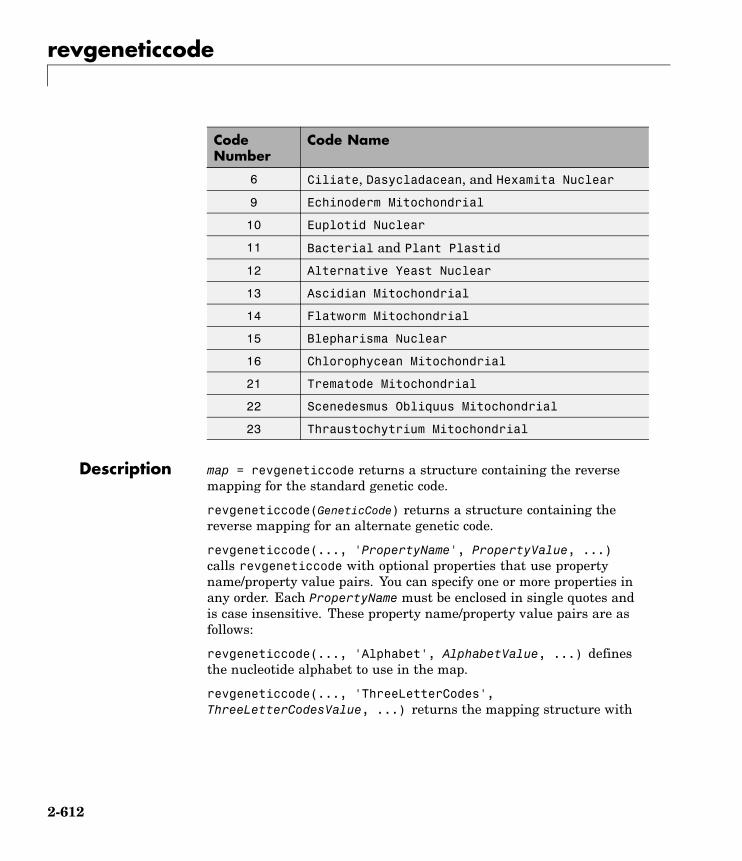
revgeneticcode
CodeNumber
Code Name
6 Ciliate, Dasycladacean, and Hexamita Nuclear
9 Echinoderm Mitochondrial
10 Euplotid Nuclear
11 Bacterial and Plant Plastid
12 Alternative Yeast Nuclear
13 Ascidian Mitochondrial
14 Flatworm Mitochondrial
15 Blepharisma Nuclear
16 Chlorophycean Mitochondrial
21 Trematode Mitochondrial
22 Scenedesmus Obliquus Mitochondrial
23 Thraustochytrium Mitochondrial
Description map = revgeneticcode returns a structure containing the reversemapping for the standard genetic code.
revgeneticcode(GeneticCode) returns a structure containing thereverse mapping for an alternate genetic code.
revgeneticcode(..., 'PropertyName', PropertyValue, ...)calls revgeneticcode with optional properties that use propertyname/property value pairs. You can specify one or more properties inany order. Each PropertyName must be enclosed in single quotes andis case insensitive. These property name/property value pairs are asfollows:
revgeneticcode(..., 'Alphabet', AlphabetValue, ...) definesthe nucleotide alphabet to use in the map.
revgeneticcode(..., 'ThreeLetterCodes',ThreeLetterCodesValue, ...) returns the mapping structure with
2-612

revgeneticcode
three-letter amino acid codes as field names instead of the defaultsingle-letter codes if ThreeLetterCodes is true.
Examples moldcode = revgeneticcode(4,'Alphabet','rna');wormcode = revgeneticcode('Flatworm Mitochondrial',...
'ThreeLetterCodes',true);
map = revgeneticcode
map =
Name: 'Standard'A: {'GCT' 'GCC' 'GCA' 'GCG'}R: {'CGT' 'CGC' 'CGA' 'CGG' 'AGA' 'AGG'}N: {'AAT' 'AAC'}D: {'GAT' 'GAC'}C: {'TGT' 'TGC'}Q: {'CAA' 'CAG'}E: {'GAA' 'GAG'}G: {'GGT' 'GGC' 'GGA' 'GGG'}H: {'CAT' 'CAC'}I: {'ATT' 'ATC' 'ATA'}L: {'TTA' 'TTG' 'CTT' 'CTC' 'CTA' 'CTG'}K: {'AAA' 'AAG'}M: {'ATG'}F: {'TTT' 'TTC'}P: {'CCT' 'CCC' 'CCA' 'CCG'}S: {'TCT' 'TCC' 'TCA' 'TCG' 'AGT' 'AGC'}T: {'ACT' 'ACC' 'ACA' 'ACG'}W: {'TGG'}Y: {'TAT' 'TAC'}V: {'GTT' 'GTC' 'GTA' 'GTG'}
Stops: {'TAA' 'TAG' 'TGA'}Starts: {'TTG' 'CTG' 'ATG'}
References [1] NCBI Web page describing genetic codes:
2-613

revgeneticcode
http://www.ncbi.nlm.nih.gov/Taxonomy/Utils/wprintgc.cgi?mode=c
See Also Bioinformatics Toolbox functions: aa2nt, aminolookup, baselookup,geneticcode, nt2aa
2-614
rmabackadj
Purpose Perform background adjustment on Affymetrix microarray probe-leveldata using Robust Multi-array Average (RMA) procedure
Syntax BackgroundAdjustedMatrix = rmabackadj(PMData)BackgroundAdjustedMatrix = rmabackadj(..., 'Method',MethodValue, ...)BackgroundAdjustedMatrix = rmabackadj(..., 'Truncate',
TruncateValue, ...)BackgroundAdjustedMatrix = rmabackadj(..., 'Showplot',
ShowplotValue, ...)
ArgumentsPMData Matrix of intensity values where each row
corresponds to a perfect match (PM) probe andeach column corresponds to an Affymetrix CEL file.(Each CEL file is generated from a separate chip.All chips should be of the same type.)
MethodValue Property to control the estimation method for thebackground adjustment model parameters. Entereither 'RMA' (to use estimation method described byBolstad, 2005) or 'MLE' (to estimate the parametersusing maximum likelihood). Default is 'RMA'.
2-615
rmabackadj
TruncateValue Property to control the background noise model.Enter either true (use a truncated Gaussiandistribution) or false (use a nontruncated Gaussiandistribution). Default is true.
ShowplotValue Property to control the plotting of a histogramshowing the distribution of PM probe intensityvalues (blue) and the convoluted probabilitydistribution function (red), with estimatedparameters. Enter either 'all' (plot a histogramfor each column or chip) or specify a subset ofcolumns (chips) by entering the column number, listof numbers, or range of numbers.
For example:
• ..., 'Showplot', 3, ...) plots theintensity values in column 3.
• ..., 'Showplot', [3,5,7], ...) plots theintensity values in columns 3, 5, and 7.
• ..., 'Showplot', 3:9, ...) plots theintensity values in columns 3 to 9.
Description BackgroundAdjustedMatrix = rmabackadj(PMData) returns thebackground adjusted values of probe intensities in the matrix, PMData.Note that each row in PMData corresponds to a perfect match (PM) probeand each column in PMData corresponds to an Affymetrix CEL file.(Each CEL file is generated from a separate chip. All chips should be ofthe same type.) Details on the background adjustment are described byBolstad, 2005.
BackgroundAdjustedMatrix = rmabackadj(..., 'PropertyName',PropertyValue, ...) defines optional properties that use propertyname/value pairs in any order. These property name/value pairs areas follows:
2-616
rmabackadj
BackgroundAdjustedMatrix = rmabackadj(..., 'Method',MethodValue, ...) controls the estimation method for the backgroundadjustment model parameters. When MethodValue is 'RMA',rmabackadj implements the estimation method described by Bolstad,2005. When MethodValue is 'MLE', rmabackadj estimates theparameters using maximum likelihood. Default is 'RMA'.
BackgroundAdjustedMatrix = rmabackadj(..., 'Truncate',TruncateValue, ...) controls the background noise model used.When TruncateValue is false, rmabackadj uses nontruncatedGaussian as the background noise model. Default is true.
BackgroundAdjustedMatrix = rmabackadj(..., 'Showplot',ShowplotValue, ...) lets you plot a histogram showing thedistribution of PM probe intensity values (blue) and the convolutedprobability distribution function (red), with estimated parameters.When ShowplotValue is 'all', rmabackadj plots a histogram for eachcolumn or chip. When ShowplotValue is a number, list of numbers,or range of numbers, rmabackadj plots a histogram for the indicatedcolumn number (chip).
For example:
• ..., 'Showplot', 3,...) plots the intensity values in column 3of Data.
• ..., 'Showplot', [3,5,7],...) plots the intensity values incolumns 3, 5, and 7 of Data.
• ..., 'Showplot', 3:9,...) plots the intensity values in columns3 to 9 of PMData.
2-617

rmabackadj
Examples 1 Load a MAT file, included with Bioinformatics Toolbox, whichcontains Affymetrix probe-level data, including pmMatrix, a matrix ofPM probe intensity values from multiple CEL files.
load prostatecancerrawdata
2 Perform background adjustment on the PM probe intensityvalues in the matrix, pmMatrix, creating a new matrix,BackgroundAdjustedMatrix.
2-618
rmabackadj
BackgroundAdjustedMatrix = rmabackadj(pmMatrix);
3 Perform background adjustment on the PM probe intensity valuesin only column 3 of the matrix, pmMatrix, creating a new matrix,BackgroundAdjustedChip3.
BackgroundAdjustedChip3 = rmabackadj(pmMatrix(:,3));
The prostatecancerrawdata.mat file used in the previous examplecontains data from Best et al., 2005.
References [1] Irizarry, R.A., Hobbs, B., Collin, F., Beazer-Barclay, Y.D., Antonellis,K.J., Scherf, U., Speed, T.P. (2003). Exploration, Normalization, andSummaries of High Density Oligonucleotide Array Probe Level Data.Biostatistics 4, 249-264.
[2] Bolstad, B. (2005). “affy: Built-in Processing Methods”http://www.bioconductor.org/repository/devel/vignette/builtinMethods.pdf
[3] Best, C.J.M., Gillespie, J.W., Yi, Y., Chandramouli, G.V.R.,Perlmutter, M.A., Gathright, Y., Erickson, H.S., Georgevich, L., Tangrea,M.A., Duray, P.H., Gonzalez, S., Velasco, A., Linehan, W.M., Matusik,R.J., Price, D.K., Figg, W.D., Emmert-Buck, M.R., and Chuaqui, R.F.(2005). Molecular alterations in primary prostate cancer after androgenablation therapy. Clinical Cancer Research 11, 6823-6834.
See Also affyinvarsetnorm, affyread, celintensityread, probelibraryinfo,probesetlink, probesetlookup, probesetvalues, quantilenorm,rmasummary
2-619

rmasummary
Purpose Calculate gene (probe set) expression values from Affymetrix microarrayprobe-level data using Robust Multi-array Average (RMA) procedure
Syntax ExpressionMatrix = rmasummary(ProbeIndices, Data)ExpressionMatrix = rmasummary(..., 'Output', OutputValue)
ArgumentsProbeIndices Column vector of probe indices. The convention
for probe indices is, for each probe set, to labeleach probe 0 to N - 1, where N is the number ofprobes in the probe set.
Data Matrix of natural-scale intensity values whereeach row corresponds to a perfect match (PM)probe and each column corresponds to anAffymetrix CEL file. (Each CEL file is generatedfrom a separate chip. All chips should be of thesame type.)
OutputValue Property to control the scale of the returned geneexpression values. OutputValue can be:
• 'log'
• 'log2'
• 'log10'
• 'natural'
• @functionname
In the last instance, the data is transformed asdefined by the function functionname. Defaultis 'log2'.
Description ExpressionMatrix = rmasummary(ProbeIndices, Data) returns gene(probe set) expression values after calculating them from natural-scaleprobe intensities in the matrix Data, using the column vector of probe
2-620
rmasummary
indices, ProbeIndices. Note that each row in Data corresponds toa perfect match (PM) probe, and each column corresponds to anAffymetrix CEL file. (Each CEL file is generated from a separate chip.All chips should be of the same type.) Note that the column vectorProbeIndices designates probes within each probe set by labeling eachprobe 0 to N - 1, where N is the number of probes in the probe set. Notethat each row in ExpressionMatrix corresponds to a gene (probe set)and each column in ExpressionMatrix corresponds to an AffymetrixCEL file, which represents a single chip.
For a given probe set n, with J probe pairs, let Yijn denote thebackground adjusted, base 2 log transformed and quantile-normalizedPM probe intensity value of chip i and probe j. Yijn follows a linearadditive model:
Yijn = Uin + Ajn + Eijn; i = 1, ..., I; j = 1, ..., J; n = 1, ..., N
where:
Uin = gene expression of the probe set n on chip i
Ajn = probe affinity effect for the jth probe in the probe set
Eijn = residual for the jth probe on the ith chip
The RMA methods assumes A1 + A2 + ... + AJ = 0 for all probe sets. Arobust procedure, median polish, is used to estimate Ui as the log scalemeasure of expression.
Note There is no column in ExpressionMatrix that contains probe setor gene information.
ExpressionMatrix = rmasummary(..., 'PropertyName',PropertyValue, ...) defines optional properties that use property
2-621
rmasummary
name/value pairs in any order. These property name/value pairs areas follows:
ExpressionMatrix = rmasummary(..., 'Output', OutputValue)controls the scale of the returned gene expression values. OutputValuecan be:
• 'log'
• 'log2'
• 'log10'
• 'natural'
• @functionname
In the last instance, the data is transformed as defined by the functionfunctionname. Default is 'log2'.
Examples 1 Load a MAT file, included with Bioinformatics Toolbox, whichcontains Affymetrix data variables, including pmMatrix, a matrix ofPM probe intensity values from multiple CEL files.
load prostatecancerrawdata
2 Perform background adjustment on the PM probe intensity valuesin the matrix, pmMatrix, using the rmabackadj function, therebycreating a new matrix, BackgroundAdjustedMatrix.
BackgroundAdjustedMatrix = rmabackadj(pmMatrix);
3 Normalize the data in BackgroundAdjustedMatrix, using thequantilenorm function.
NormMatrix = quantilenorm(BackgroundAdjustedMatrix);
4 Calculate gene expression values from the probe intensities inNormMatrix, creating a new matrix, ExpressionMatrix. (You will
2-622

rmasummary
use the probeIndices column vector provided to supply informationon the probe indices.)
ExpressionMatrix = rmasummary(probeIndices, NormMatrix);
The prostatecancerrawdata.mat file used in the previous examplecontains data from Best et al., 2005.
References [1] Irizarry, R.A., Hobbs, B., Collin, F., Beazer-Barclay, Y.D., Antonellis,K.J., Scherf, U., Speed, T.P. (2003). Exploration, Normalization, andSummaries of High Density Oligonucleotide Array Probe Level Data.Biostatistics. 4, 249-264.
[2] Mosteller, F., and Tukey, J. (1977). Data Analysis and Regression(Reading, Massachusetts: Addison-Wesley Publishing Company), pp.165-202.
[3] Best, C.J.M., Gillespie, J.W., Yi, Y., Chandramouli, G.V.R.,Perlmutter, M.A., Gathright, Y., Erickson, H.S., Georgevich, L., Tangrea,M.A., Duray, P.H., Gonzalez, S., Velasco, A., Linehan, W.M., Matusik,R.J., Price, D.K., Figg, W.D., Emmert-Buck, M.R., and Chuaqui, R.F.(2005). Molecular alterations in primary prostate cancer after androgenablation therapy. Clinical Cancer Research 11, 6823-6834.
See Also affyinvarsetnorm, celintensityread, mainvarsetnorm, malowess,manorm, quantilenorm, rmabackadj
2-623

rna2dna
Purpose Convert RNA sequence of nucleotides to DNA sequence
Syntax SeqDNA = rna2dna(SeqRNA)
ArgumentsSeqRNA Nucleotide sequence for RNA. Enter a character string
with the characters A, C, U, G, and the ambiguousnucleotide bases N, R, Y, K, M, S, W, B, D, H, and V.
Description SeqDNA = rna2dna(SeqRNA) converts any uracil nucleotides in an RNAsequence into thymine (U-->T), and returns in the same format as DNA.For example, if the RNA sequence is an integer sequence then so isSeqRNA.
Example rna2dna('ACGAUGAGUCAUGCUU')
ans =ACGATGAGTCATGCTT
See Also Bioinformatics Toolbox function: dna2rna
MATLAB functions: strrep, regexp
2-624
scfread
Purpose Read trace data from SCF file
Syntax Sample = scfread('File')[Sample, Probability] = scfread('File')[Sample, Probability, Comments] = scfread('File')[A, C, T, G] = scfread ('File')[A, C, T, G, ProbA, ProbC, ProbG, ProbT] = scfread ('File')[A, C, T, G, ProbA, ProbC, ProbG, ProbT, Comments, PkIndex,
Base] = scfread ('File')
Arguments File SCF formatted file. Enter a file name or a path and filename.
Description scfread reads data from an SCF formatted file into MATLABstructures.
Sample = scfread('File') reads an SCF formatted file and returnsthe sample data in the structure Sample, which contains the followingfields:
Field Description
A Column vector containing intensity of A fluorescencetag
C Column vector containing intensity of C fluorescencetag
G Column vector containing intensity of G fluorescencetag
T Column vector containing intensity of T fluorescencetag
[Sample, Probability] = scfread('File') also returns theprobability data in the structure Probability, which contains thefollowing fields:
2-625
scfread
Field Description
peak_index Column vector containing the position in the SCF filefor the start of the data for each peak
prob_A Column vector containing the probability of each basein the sequence being an A
prob_C Column vector containing the probability of each basein the sequence being a C
prob_G Column vector containing the probability of each basein the sequence being a G
prob_T Column vector containing the probability of each basein the sequence being a T
base Column vector containing the called bases for thesequence
[Sample, Probability, Comments] = scfread('File') also returnsthe comment information from the SCF file in a character arrayComments.
[A, C, T, G] = scfread ('File') returns the sample data for thefour bases in separate variables.
[A, C, T, G, ProbA, ProbC, ProbG, ProbT] = scfread ('File')also returns the probabilities data for the four bases in separatevariables.
[A, C, T, G, ProbA, ProbC, ProbG, ProbT, Comments,PkIndex, Base] = scfread ('File') also returns the peak indicesand called bases in separate variables.
SCF files store data from DNA sequencing instruments. Eachfile includes sample data, sequence information, and the relativeprobabilities of each of the four bases. For more information on SCFfiles, see
http://www.mrc-lmb.cam.ac.uk/pubseq/manual/formats_unix_2.html
2-626

scfread
Examples [sampleStruct, probStruct, Comments] = scfread('sample.scf')sampleStruct =
A: [10827x1 double]C: [10827x1 double]G: [10827x1 double]T: [10827x1 double]
probStruct =
peak_index: [742x1 double]prob_A: [742x1 double]prob_C: [742x1 double]prob_G: [742x1 double]prob_T: [742x1 double]
base: [742x1 char]
Comments =
SIGN=A=121,C=103,G=119,T=82SPAC= 16.25PRIM=0MACH=Arkansas_SN312DYEP=DT3700POP5{BD}v2.mobNAME=HCIUP1D61207LANE=6GELN=PROC=RTRK=CONV=phred version=0.990722.hCOMM=SRCE=ABI 373A or 377
See Also Bioinformatics Toolbox functions: genbankread, traceplot
2-627
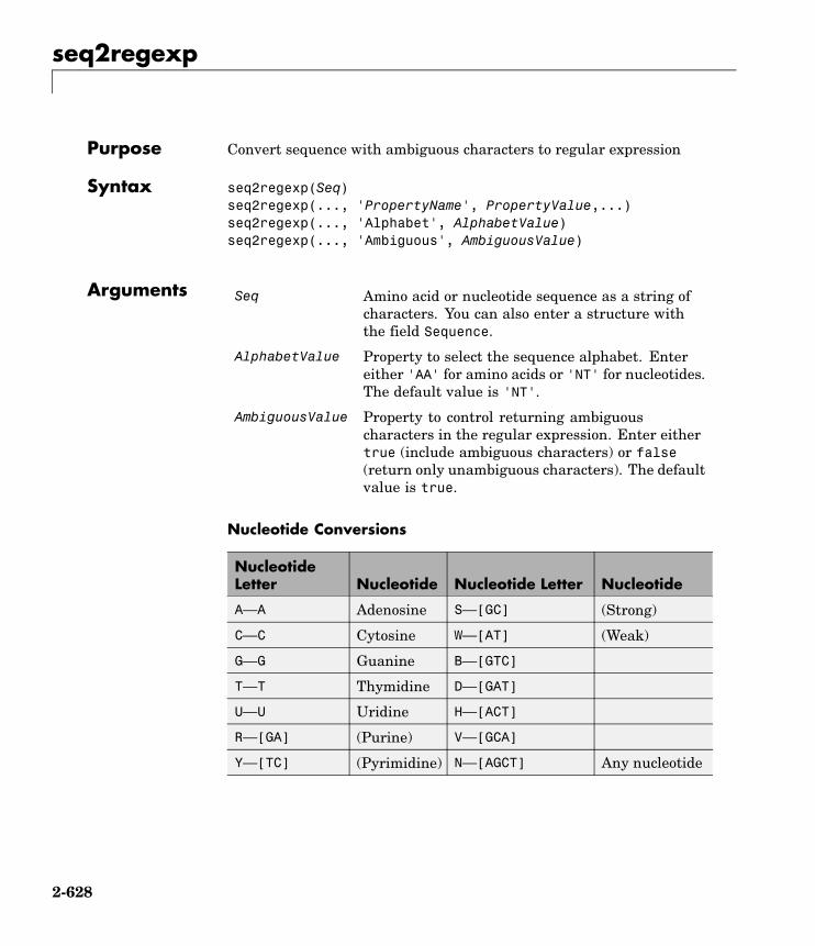
seq2regexp
Purpose Convert sequence with ambiguous characters to regular expression
Syntax seq2regexp(Seq)seq2regexp(..., 'PropertyName', PropertyValue,...)seq2regexp(..., 'Alphabet', AlphabetValue)seq2regexp(..., 'Ambiguous', AmbiguousValue)
Arguments Seq Amino acid or nucleotide sequence as a string ofcharacters. You can also enter a structure withthe field Sequence.
AlphabetValue Property to select the sequence alphabet. Entereither 'AA' for amino acids or 'NT' for nucleotides.The default value is 'NT'.
AmbiguousValue Property to control returning ambiguouscharacters in the regular expression. Enter eithertrue (include ambiguous characters) or false(return only unambiguous characters). The defaultvalue is true.
Nucleotide Conversions
NucleotideLetter Nucleotide Nucleotide Letter Nucleotide
A—A Adenosine S—[GC] (Strong)
C—C Cytosine W—[AT] (Weak)
G—G Guanine B—[GTC]
T—T Thymidine D—[GAT]
U—U Uridine H—[ACT]
R—[GA] (Purine) V—[GCA]
Y—[TC] (Pyrimidine) N—[AGCT] Any nucleotide
2-628
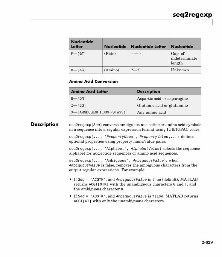
seq2regexp
NucleotideLetter Nucleotide Nucleotide Letter Nucleotide
K—[GT] (Keto) - — - Gap ofindeterminatelength
M—[AC] (Amino) ?—? Unknown
Amino Acid Conversion
Amino Acid Letter Description
B—[DN] Aspartic acid or asparagine
Z—[EQ] Glutamic acid or glutamine
X—[ARNDCQEGHILKMFPSTWYV] Any amino acid
Description seq2regexp(Seq) converts ambiguous nucleotide or amino acid symbolsin a sequence into a regular expression format using IUB/IUPAC codes.
seq2regexp(..., 'PropertyName', PropertyValue,...) definesoptional properties using property name/value pairs.
seq2regexp(..., 'Alphabet', AlphabetValue) selects the sequencealphabet for nucleotide sequences or amino acid sequences.
seq2regexp(..., 'Ambiguous', AmbiguousValue), whenAmbiguousValue is false, removes the ambiguous characters from theoutput regular expressions. For example:
• If Seq = 'ACGTK', and AmbiguousValue is true (default), MATLABreturns ACGT[GTK] with the unambiguous characters G and T, andthe ambiguous character K.
• If Seq = 'ACGTK', and AmbiguousValue is false, MATLAB returnsACGT[GT] with only the unambiguous characters.
2-629

seq2regexp
Example 1 Convert a nucleotide sequence into a regular expression.
seq2regexp('ACWTMAN')
ans =AC[ATW]T[ACM]A[ACGTRYKMSWBDHVN]
2 Remove ambiguous characters from the regular expression.
seq2regexp('ACWTMAN', 'ambiguous', false)
ans =AC[AT]T[AC]A[ACGT]
See Also Bioinformatics Toolbox functions: restrict, seqwordcount
MATLAB functions: regexp, regexpi
2-630

seqcomplement
Purpose Calculate complementary strand of nucleotide sequence
Syntax SeqC = seqcomplement(SeqNT)
ArgumentsSeqNT Enter either a character string with the characters A,
T (U), G, C, and ambiguous characters R, Y, K, M, S, W,B, D, H, V, N, or a vector of integers. You can also entera structure with the field Sequence.
Description SeqC = seqcomplement(SeqNT) calculates the complementary strand(A-->T, C-->G, G-->C, T-->A) of a DNA sequence and returns a sequence inthe same format as SeqNT. For example, if SeqNT is an integer sequencethen so is SeqC.
Example Return the complement of a DNA nucleotide sequence.
s = 'ATCG';seqcomplement(s)
ans =TAGC
See Also Bioinformatics Toolbox functions seqrcomplement, seqreverse,seqtool
2-631
seqconsensus
Purpose Calculate consensus sequence
Syntax CSeq = seqconsensus(Seqs)[CSeq, Score] = seqconsensus(Seqs)CSeq = seqconsensus(Profile)seqconsensus(..., 'PropertyName', PropertyValue,...)seqconsensus(..., 'ScoringMatrix', ScoringMatrixValue)
ArgumentsSeqs Set of multiply aligned amino acid or
nucleotide sequences. Enter an array ofstrings, a cell array of strings, or an array ofstructures with the field Sequence.
Profile Sequence profile. Enter a profile from thefunction seqprofile. Profile is a matrix ofsize [20 (or 4) x Sequence Length] withthe frequency or count of amino acids (ornucleotides) for every position. Profile canalso have 21 (or 5) rows if gaps are includedin the consensus.
ScoringMatrixValue Scoring matrix. The default value isBLOSUM50 for amino acid sequences or NUC44for nucleotide sequences. ScoringMatrixcan also be a 21x21, 5x5, 20x20, or 4x4numeric array. For the gap-included cases,gap scores (last row/column) are set tomean(diag(ScoringMatrix))for a gapmatching with another gap, and set tomean(nodiag(ScoringMatrix)) for a gapmatching with another symbol
Description CSeq = seqconsensus(Seqs), for a multiply aligned set of sequences(Seqs), returns a string with the consensus sequence (CSeq). Thefrequency of symbols (20 amino acids, 4 nucleotides) in the set ofsequences is determined with the function seqprofile. For ambiguous
2-632

seqconsensus
nucleotide or amino acid symbols, the frequency or count is added tothe standard set of symbols.
[CSeq, Score] = seqconsensus(Seqs) returns the conservationscore of the consensus sequence. Scores are computed with the scoringmatrix BLOSUM50 for amino acids or NUC44 for nucleotides. Scores arethe average euclidean distance between the scored symbol and theM-dimensional consensus value. M is the size of the alphabet. Theconsensus value is the profile weighted by the scoring matrix.
CSeq = seqconsensus(Profile) returns a string with the consensussequence (CSeq) from a sequence profile (Profile).
seqconsensus(..., 'PropertyName', PropertyValue,...) definesoptional properties using property name/value pairs.
seqconsensus(..., 'ScoringMatrix', ScoringMatrixValue)specifies the scoring matrix.
The following input parameters are analogous to the functionseqprofile when the alphabet is restricted to 'AA' or 'NT'.
seqconsensus(..., 'Alphabet', AlphabetValue)
seqconsensus(..., 'Gaps', GapsValue)
seqconsensus(..., 'Ambiguous', AmbiguousValue)
seqconsensus(..., 'Limits', LimitsValue)
Examples seqs = fastaread('pf00002.fa');[C,S] = seqconsensus(seqs,'limits',[50 60],'gaps','all')
See Also Bioinformatics Toolbox functions fastaread, multialignread,profalign, seqdisp, seqprofile
2-633

seqdisp
Purpose Format long sequence output for easy viewing
Syntax seqdisp(Seq)seqdisp(..., 'PropertyName', PropertyValue,...)seqdisp(..., 'Row', RowValue)seqdisp(..., 'Column', ColumnValue)seqdisp(..., 'ShowNumbers', ShowNumbersValue)
ArgumentsSeq Nucleotide or amino acid sequence. Enter a character
array, a FASTA file name, or a MATLAB structurewith the field Sequence. Multiply aligned sequencesare allowed.
FASTA files can have the file extension fa, fasta,fas, fsa, or fst.
Row Property to select the length of each row. Enter aninteger. The default length is 60.
Column Property to select the column width or number ofsymbols before displaying a space. Enter an integer.The default column width is 10.
ShowNumbers Property to control displaying numbers at the start ofeach row. Enter either true (default) to show numbersor false to hide numbers.
Description seqdisp(Seq) displays a sequence (Seq) in rows with a default rowlength of 60 and a default column width of 10.
seqdisp(..., 'PropertyName', PropertyValue,...) definesoptional properties using property name/value pairs.
seqdisp(..., 'Row', RowValue) specifies the length of each row forthe displayed sequence.
2-634

seqdisp
seqdisp(..., 'Column', ColumnValue) specifies the number ofletters to display before adding a space. Row must be larger than andevenly divisible by Column.
seqdisp(..., 'ShowNumbers', ShowNumbersValue) whenShowNumbers is false, turns off the position numbers at the start ofeach row off.
Examples Read sequence information from the GenBank database. Display thesequence in rows with 50 letters, and within a row, separate every 10letters with a space.
mouseHEXA = getgenbank('AK080777');seqdisp(mouseHEXA, 'Row', 50, 'Column', 10)
Create and save a FASTA file with two sequences, and then display it.
hdr = ['Sequence A'; 'Sequence B'];seq = ['TAGCTGRCCAAGGCCAAGCGAGCTTN';'ATCGACYGGTTCCGGTTCGCTCGAAN']fastawrite('local.fa', hdr, seq);seqdisp('local.fa', 'ShowNumbers', false')
ans =>Sequence A1 TAGCTGRCCA AGGCCAAGCG AGCTTN
>Sequence B1 ATCGACYGGT TCCGGTTCGC TCGAAN
See Also Bioinformatics Toolbox functions: multialignread, seqconsensus,seqlogo, seqprofile, seqshoworfs, seqshowwords, seqtool,getgenbank
2-635

seqdotplot
Purpose Create dot plot of two sequences
Syntax seqdotplot (Seq1, Seq2)seqdotplot(Seq1,Seq2, Window, Number)Matches = seqdotplot(...)[Matches, Matrix] = seqdotplot(...)
ArgumentsSeq1, Seq2 Nucleotide or amino acid sequences.
Enter two character strings. Do not entera vector of integers. You can also enter astructure with the field Sequence.
Window Enter an integer for the size of a window.
Number Enter an integer for the number ofcharacters within the window thatmatch.
Description seqdotplot (Seq1, Seq2) plots a figure that visualizes the matchbetween two sequences.
seqdotplot(Seq1,Seq2, Window, Number) plots sequence matcheswhen there are at least Number matches in a window of size Window.
When plotting nucleotide sequences, start with a Window of 11 andNumber of 7.
Matches = seqdotplot(...) returns the number of dots in the dotplot matrix.
[Matches, Matrix] = seqdotplot(...) returns the dotplot as asparse matrix.
Examples This example shows the similarities between the prion protein (PrP)nucleotide sequences of two ruminants, the moufflon and the goldentakin.
moufflon = getgenbank('AB060288','Sequence',true);
2-636
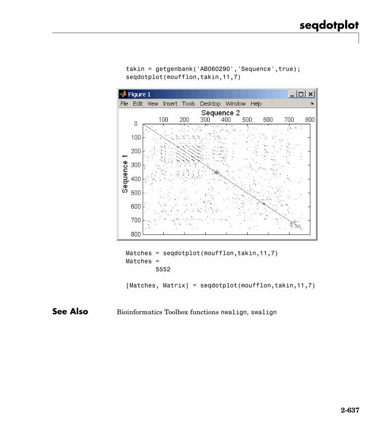
seqdotplot
takin = getgenbank('AB060290','Sequence',true);seqdotplot(moufflon,takin,11,7)
Matches = seqdotplot(moufflon,takin,11,7)Matches =
5552
[Matches, Matrix] = seqdotplot(moufflon,takin,11,7)
See Also Bioinformatics Toolbox functions nwalign, swalign
2-637
seqinsertgaps
Purpose Insert gaps into nucleotide or amino acid sequence
Syntax NewSeq = seqinsertgaps(Seq, Positions)NewSeq = seqinsertgaps(Seq, GappedSeq)NewSeq = seqinsertgaps(Seq, GappedSeq, Relationship)
Arguments Seq Either of the following:• String specifying a nucleotide or amino acid
sequence
• MATLAB structure containing a Sequence field
Positions Vector of integers to specify the positions in Seqbefore which to insert a gap.
GappedSeq Either of the following:• String specifying a nucleotide or amino acid
sequence
• MATLAB structure containing a Sequence field
Relationship Integer specifying the relationship between Seq andGappedSeq. Choices are:
• 1 — Both sequences use the same alphabet, that isboth are nucleotide sequences or both are aminoacid sequences.
• 3 — Seq contains nucleotides representing codonsand GappedSeq contains amino acids (default).
ReturnValues
NewSeq Sequence with gaps inserted, represented by a stringspecifying a nucleotide or amino acid sequence.
2-638
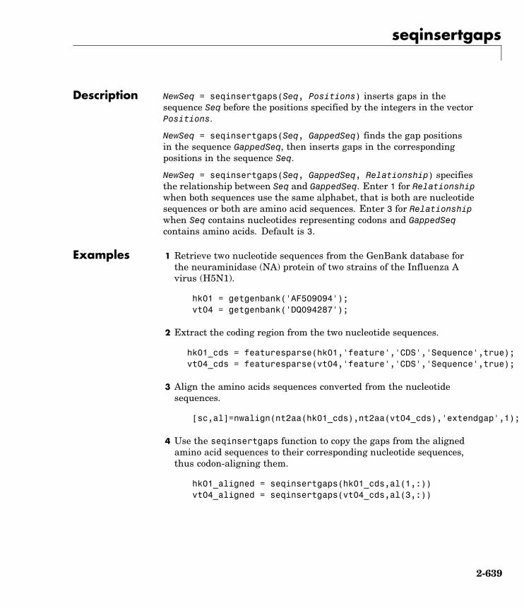
seqinsertgaps
Description NewSeq = seqinsertgaps(Seq, Positions) inserts gaps in thesequence Seq before the positions specified by the integers in the vectorPositions.
NewSeq = seqinsertgaps(Seq, GappedSeq) finds the gap positionsin the sequence GappedSeq, then inserts gaps in the correspondingpositions in the sequence Seq.
NewSeq = seqinsertgaps(Seq, GappedSeq, Relationship) specifiesthe relationship between Seq and GappedSeq. Enter 1 for Relationshipwhen both sequences use the same alphabet, that is both are nucleotidesequences or both are amino acid sequences. Enter 3 for Relationshipwhen Seq contains nucleotides representing codons and GappedSeqcontains amino acids. Default is 3.
Examples 1 Retrieve two nucleotide sequences from the GenBank database forthe neuraminidase (NA) protein of two strains of the Influenza Avirus (H5N1).
hk01 = getgenbank('AF509094');vt04 = getgenbank('DQ094287');
2 Extract the coding region from the two nucleotide sequences.
hk01_cds = featuresparse(hk01,'feature','CDS','Sequence',true);vt04_cds = featuresparse(vt04,'feature','CDS','Sequence',true);
3 Align the amino acids sequences converted from the nucleotidesequences.
[sc,al]=nwalign(nt2aa(hk01_cds),nt2aa(vt04_cds),'extendgap',1);
4 Use the seqinsertgaps function to copy the gaps from the alignedamino acid sequences to their corresponding nucleotide sequences,thus codon-aligning them.
hk01_aligned = seqinsertgaps(hk01_cds,al(1,:))vt04_aligned = seqinsertgaps(vt04_cds,al(3,:))
2-639

seqinsertgaps
5 Once you have code aligned the two sequences, you can usethem as input to other functions such as dnds, which calculatesthe synonymous and nonsynonymous substitutions rates of thecodon-aligned nucleotide sequences. By setting Verbose to true, youcan also display the codons considered in the computations and theiramino acid translations.
[dn,ds] = dnds(hk01_aligned,vt04_aligned,'verbose',true)
See Also Bioinformatics Toolbox functions: dnds, dndsml, int2aa, int2nt
2-640
seqlinkage
Purpose Construct phylogenetic tree from pair-wise distances
Syntax Tree = seqlinkage(Dist)Tree = seqlinkage(Dist, Method)Tree = seqlinkage(Dist, Method, Names)
ArgumentsDist Matrix or vector of pair-wise distances, such as
returned by the seqpdist function.
Method String that specifies a distance method. Choices are:
• 'single'
• 'complete'
• 'average' (default)
• 'weighted'
• 'centroid'
• 'median'
Names Property to use alternative labels for leaf nodes.Enter a vector of structures, with the fields 'Header'or 'Name', or a cell array of strings. In both cases thenumber of elements you provide must comply withthe number of samples used to generate the pair-wisedistances in Dist.
Description Tree = seqlinkage(Dist) returns a phylogenetic tree object fromthe pair-wise distances, Dist, between the species or products. Distis a matrix or vector of pair-wise distances, such as returned by theseqpdist function.
Tree = seqlinkage(Dist, Method) creates a phylogenetic tree objectusing a specified patristic distance method. The available methods are:
2-641
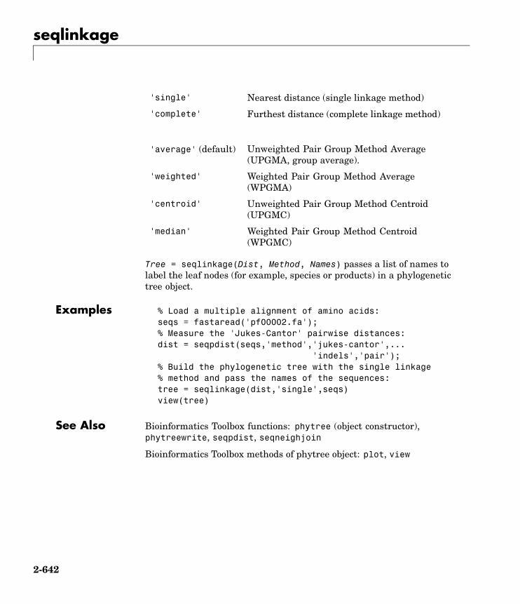
seqlinkage
'single' Nearest distance (single linkage method)
'complete' Furthest distance (complete linkage method)
'average' (default) Unweighted Pair Group Method Average(UPGMA, group average).
'weighted' Weighted Pair Group Method Average(WPGMA)
'centroid' Unweighted Pair Group Method Centroid(UPGMC)
'median' Weighted Pair Group Method Centroid(WPGMC)
Tree = seqlinkage(Dist, Method, Names) passes a list of names tolabel the leaf nodes (for example, species or products) in a phylogenetictree object.
Examples % Load a multiple alignment of amino acids:seqs = fastaread('pf00002.fa');% Measure the 'Jukes-Cantor' pairwise distances:dist = seqpdist(seqs,'method','jukes-cantor',...
'indels','pair');% Build the phylogenetic tree with the single linkage% method and pass the names of the sequences:tree = seqlinkage(dist,'single',seqs)view(tree)
See Also Bioinformatics Toolbox functions: phytree (object constructor),phytreewrite, seqpdist, seqneighjoin
Bioinformatics Toolbox methods of phytree object: plot, view
2-642
seqlogo
Purpose Display sequence logo for nucleotide or amino acid sequences
Syntax seqlogo(Seqs)seqlogo(Profile)DisplayInfo = seqlogo(Seqs)seqlogo(..., 'Displaylogo', DisplaylogoValue, ...)seqlogo(..., 'Alphabet', AlphabetValue, ...)seqlogo(..., 'Startat', StartatValue, ...)seqlogo(..., 'Endat', EndatValue, ...)seqlogo(..., 'SSCorrection', SSCorrectionValue, ...)
Arguments Seqs Set of pair-wise or multiply aligned nucleotideor amino acid sequences, represented by anyof the following:• Character array
• Cell array of strings
• Array of structures containing a Sequencefield
Profile Sequence profile distribution matrix with thefrequency of nucleotides or amino acids forevery column in the multiple alignment, suchas returned by the seqprofile function.
The size of the frequency distribution matrixis:
• For nucleotides — [4 x sequence length]
• For amino acids — [20 x sequencelength]
If gaps were included, Profile may have 5rows (for nucleotides) or 21 rows (for aminoacids), but seqlogo ignores gaps.
2-643
seqlogo
DisplaylogoValue Controls the display of a sequence logo.Choices are true (default) or false.
AlphabetValue String specifying the type of sequence(nucleotide or amino acid). Choices are 'NT'(default) or'AA'.
StartatValue Positive integer that specifies the startingposition for the sequences in Seqs. Defaultstarting position is 1.
EndatValue Positive integer that specifies the endingposition for the sequences in Seqs. Defaultending position is the maximum length of thesequences in Seqs.
SSCorrectionValue Controls the use of small sample correction inthe estimation of the number of bits. Choicesare true (default) or false.
ReturnValues
DisplayInfo Cell array containing the symbol list in Seqsand the weight matrix used to graphicallydisplay the sequence logo.
Description seqlogo(Seqs) displays a sequence logo for Seqs, a set of alignedsequences. The logo graphically displays the sequence conservationat a particular position in the alignment of sequences, measured inbits. The maximum sequence conservation per site is log2(4) bits fornucleotide sequences and log2(20) bits for amino acid sequences. Ifthe sequence conservation value is zero or negative, no logo is displayedin that position.
seqlogo(Profile) displays a sequence logo for Profile, a sequenceprofile distribution matrix with the frequency of nucleotides or aminoacids for every column in the multiple alignment, such as returned bythe seqprofile function.
2-644

seqlogo
Color Code for Nucleotides
Nucleotide Color
A Green
C Blue
G Yellow
T, U Red
Other Purple
Color Code for Amino Acids
Amino Acid ChemicalProperty
Color
G S T Y C Q N Polar Green
A V L I P W F M Hydrophobic Orange
D E Acidic Red
K R H Basic Blue
Other — Tan
DisplayInfo = seqlogo(Seqs)returns a cell array of unique symbolsin a sequence (Seqs) and the information weight matrix used tographically display the logo.
seqlogo(Seqs, ...'PropertyName', PropertyValue, ...) callsseqpdist with optional properties that use property name/propertyvalue pairs. You can specify one or more properties in any order. EachPropertyName must be enclosed in single quotation marks and is caseinsensitive. These property name/property value pairs are as follows:
seqlogo(..., 'Displaylogo', DisplaylogoValue, ...) controlsthe display of a sequence logo. Choices are true (default) or false.
2-645
seqlogo
seqlogo(..., 'Alphabet', AlphabetValue, ...) specifies the typeof sequence (nucleotide or amino acid). Choices are 'NT' (default)or'AA'.
Note If you provide amino acid sequences to seqlogo, you must setAlphabet to 'AA'.
seqlogo(..., 'Startat', StartatValue, ...) specifies the startingposition for the sequences in Seqs. Default starting position is 1.
seqlogo(..., 'Endat', EndatValue, ...) specifies the endingposition for the sequences in Seqs. Default ending position is themaximum length of the sequences in Seqs.
seqlogo(..., 'SSCorrection', SSCorrectionValue, ...) controlsthe use of small sample correction in the estimation of the number ofbits. Choices are true (default) or false.
Note A simple calculation of bits tends to overestimate theconservation at a particular location. To compensate for thisoverestimation, when SSCorrection is set to true, a rough estimateis applied as an approximate correction. This correction works betterwhen the number of sequences is greater than 50.
Examples Displaying a Sequence Logo for a Nucleotide Sequence
1 Create a series of aligned nucleotide sequences.
S = {'ATTATAGCAAACTA',...'AACATGCCAAAGTA',...'ATCATGCAAAAGGA'}
2 Display the sequence logo.
2-646

seqlogo
seqlogo(S)
3 Notice that correction for small samples prevents you from seeingcolumns with information equal to log2(4) = 2 bits, but you canturn this adjustment off.
seqlogo(S,'sscorrection',false)
Displaying a Sequence Logo for an Amino Acid Sequence
1 Create a series of aligned amino acid sequences.
S2 = {'LSGGQRQRVAIARALAL',...'LSGGEKQRVAIARALMN',...
2-647
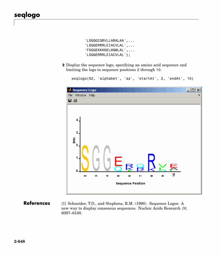
seqlogo
'LSGGQIQRVLLARALAA',...'LSGGERRRLEIACVLAL',...'FSGGEKKKNELWQMLAL',...'LSGGERRRLEIACVLAL'};
2 Display the sequence logo, specifying an amino acid sequence andlimiting the logo to sequence positions 2 through 10.
seqlogo(S2, 'alphabet', 'aa', 'startAt', 2, 'endAt', 10)
References [1] Schneider, T.D., and Stephens, R.M. (1990). Sequence Logos: Anew way to display consensus sequences. Nucleic Acids Research 18,6097–6100.
2-648

seqlogo
See Also Bioinformatics Toolbox functions: seqconsensus, seqdisp, seqprofile
2-649
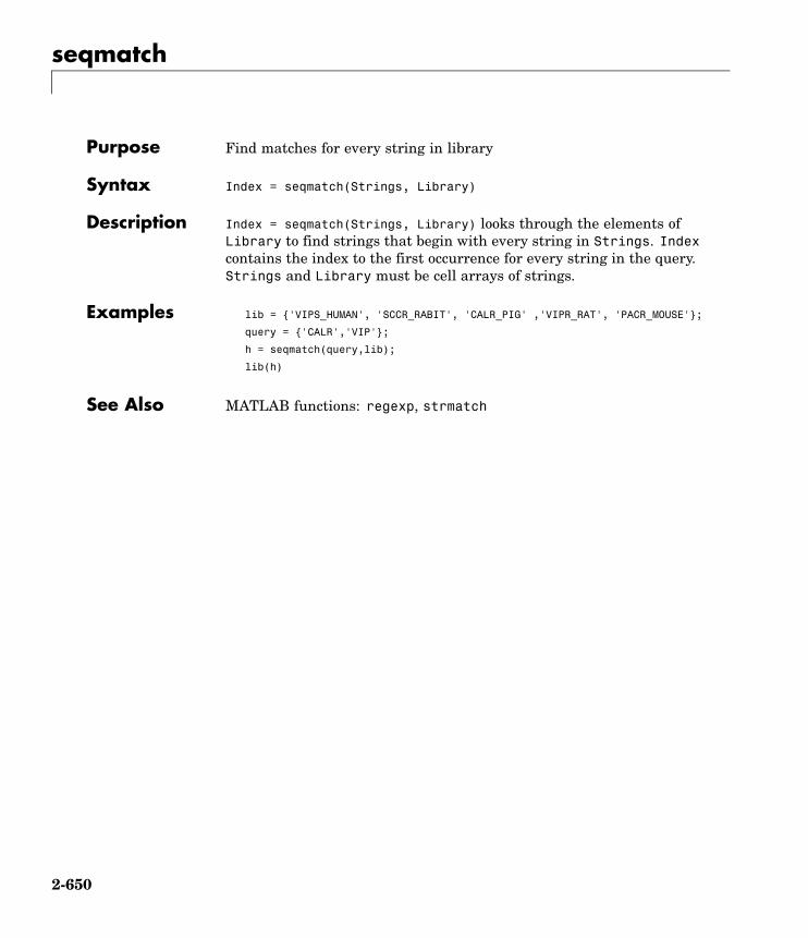
seqmatch
Purpose Find matches for every string in library
Syntax Index = seqmatch(Strings, Library)
Description Index = seqmatch(Strings, Library) looks through the elements ofLibrary to find strings that begin with every string in Strings. Indexcontains the index to the first occurrence for every string in the query.Strings and Library must be cell arrays of strings.
Examples lib = {'VIPS_HUMAN', 'SCCR_RABIT', 'CALR_PIG' ,'VIPR_RAT', 'PACR_MOUSE'};
query = {'CALR','VIP'};
h = seqmatch(query,lib);
lib(h)
See Also MATLAB functions: regexp, strmatch
2-650
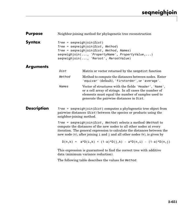
seqneighjoin
Purpose Neighbor-joining method for phylogenetic tree reconstruction
Syntax Tree = seqneighjoin(Dist)Tree = seqneighjoin(Dist, Method)Tree = seqneighjoin(Dist, Method, Names)seqneighjoin(..., 'PropertyName', PropertyValue,...)seqneighjoin(..., 'Reroot', RerootValue)
ArgumentsDist Matrix or vector returned by the seqpdist function
Method Method to compute the distances between nodes. Enter'equivar' (default), 'firstorder', or 'average'.
Names Vector of structures with the fields 'Header', 'Name',or a cell array of strings. In all cases the number ofelements must equal the number of samples used togenerate the pairwise distances in Dist.
Description Tree = seqneighjoin(Dist) computes a phylogenetic tree object frompairwise distances (Dist) between the species or products using theneighbor-joining method.
Tree = seqneighjoin(Dist, Method) selects a method (Method) tocompute the distances of the new nodes to all other nodes at everyiteration. The general expression to calculate the distances between thenew node (n), after joining i and j and all other nodes (k), is given by
D(n,k) = a*D(i,k) + (1-a)*D(j,k) - a*D(n,i) - (1-a)*D(n,j)
This expression is guaranteed to find the correct tree with additivedata (minimum variance reduction).
The following table describes the values for Method.
2-651

seqneighjoin
'equivar'(default)
Assumes equal variance and independence ofevolutionary distance estimates (a = 1/2). Such asin Studier and Keppler, JMBE (1988).
'firstorder' Assumes a first-order model of the variances andcovariances of evolutionary distance estimates, 'a'is adjusted at every iteration to a value between 0and 1. Such as in Gascuel, JMBE (1997).
'average' New distances are the weighted average of previousdistances while the branch distances are ignored.
D(n,k) = [ D(i,k) + D(j,k) ] /2
As in the original neighbor-joining algorithm bySaitou and Nei, JMBE (1987).
Tree = seqneighjoin(Dist, Method, Names) passes a list ofnames (Names) to label the leaf nodes (e.g., species or products) in thephylogenetic tree object.
seqneighjoin(..., 'PropertyName', PropertyValue,...) definesoptional properties using property name/value pairs.
seqneighjoin(..., 'Reroot', RerootValue), when RerootValue isfalse, excludes rerooting the resulting tree. This is useful for observingthe original linkage order followed by the algorithm. By defaultseqneighjoin reroots the resulting tree using the midpoint method.
Examples 1 Load a multiple alignment of amino acids.
seqs = fastaread('pf00002.fa');
2 Measure the Jukes-Cantor pair-wise distances.
dist = seqpdist(seqs,'method','jukes-cantor','indels','pair');
3 Build the phylogenetic using the neighbor-joining algorithm.
2-652
seqneighjoin
tree = seqneighjoin(dist,'equivar',seqs)view(tree)
References [1] Saitou, N., and Nei, M. (1987). The neighbor-joining method: A newmethod for reconstructing phylogenetic trees. Molecular Biology andEvolution 4(4), 406–425.
[2] Gascuel, O. (1997). BIONJ: An improved version of the NJ algorithmbased on a simple model of sequence data. Molecular Biology andEvolution 14 685–695.
[3] Studier, J.A., Keppler, K.J. (1988). A note on the neighbor-joiningalgorithm of Saitou and Nei. Molecular Biology and Evolution 5(6)729–731.
See Also Bioinformatics Toolbox functions: multialign, phytree (objectconstructor), seqlinkage (alternative method to create a phylogenetictree), seqpdist
Methods of phytree object: reroot, view
2-653

seqpdist
Purpose Calculate pair-wise distance between sequences
Syntax D = seqpdist(Seqs)D = seqpdist(Seqs, ...'Method', MethodValue, ...)D = seqpdist(Seqs, ...'Indels', IndelsValue, ...)D = seqpdist(Seqs, ...'Optargs', OptargsValue, ...)D = seqpdist(Seqs, ...'PairwiseAlignment',
PairwiseAlignmentValue, ...)D = seqpdist(Seqs, ...'JobManager', JobManagerValue, ...)D = seqpdist(Seqs, ...'WaitInQueue', WaitInQueueValue, ...)D = seqpdist(Seqs, ...'SquareForm', SquareFormValue, ...)D = seqpdist(Seqs, ...'Alphabet', AlphabetValue, ...)D = seqpdist(Seqs, ...'ScoringMatrix', ScoringMatrixValue,
...)D = seqpdist(Seqs, ...'Scale', ScaleValue, ...)D = seqpdist(Seqs, ...'GapOpen', GapOpenValue, ...)D = seqpdist(Seqs, ...'ExtendGap', ExtendGapValue, ...)
Arguments Seqs Any of the following:• Cell array containing nucleotide or
amino acid sequences
• Vector of structures containing aSequence field
• Matrix of characters, in which each rowcorresponds to a nucleotide or aminoacid sequence
MethodValue String that specifies the method forcalculating pair-wise distances. Default isJukes-Cantor.
IndelsValue String that specifies how to treat siteswith gaps. Default is score.
2-654
seqpdist
OptargsValue String or cell array specifying one or moreinput arguments required or acceptedby the distance method specified by theMethod property.
PairwiseAlignmentValue Controls the global pair-wise alignmentof input sequences (using the nwalignfunction), while ignoring the multiplealignment of the input sequences (if any).Choices are true or false. Default is:
• true — When all input sequences donot have the same length.
• false — When all input sequenceshave the same length.
Tip If your input sequences have thesame length, seqpdist will assume theyaligned. If they are not aligned, do one ofthe following:
• Align the sequences before passingthem to seqpdist, for example, usingthe multialign function.
• Set PairwiseAlignment to true whenusing seqpdist.
2-655

seqpdist
JobManagerValue A jobmanager object, such as returnedby the Distributed Computing Toolboxfunction findResource, that represents anavailable distributed MATLAB resource.Specifying this property distributespair-wise alignments into a cluster ofcomputers using Distributed ComputingToolbox. You must have DistributedComputing Toolbox to use this property.
WaitInQueueValue Controls whether seqpdist waits fora distributed MATLAB resource tobe available when you have set theJobManager property. Choices are trueor false (default). You must haveDistributed Computing Toolbox to use thisproperty.
SquareFormValue Controls the conversion of the output intoa square matrix. Choices are true orfalse (default).
AlphabetValue String specifying the type of sequence(nucleotide or amino acid). Choices are'NT' or 'AA' (default).
2-656

seqpdist
ScoringMatrixValue String specifying the scoring matrix touse for the global pair-wise alignment.Choices for amino acid sequences are:
• 'PAM40'
• 'PAM250'
• 'DAYHOFF'
• 'GONNET'
• 'BLOSUM30' increasing by 5 up to'BLOSUM90'
• 'BLOSUM62'
• 'BLOSUM100'
Default is:
• 'NUC44' (when AlphabetValue equals'NT')
• 'BLOSUM50' (when AlphabetValueequals 'AA')
ScaleValue Positive value that specifies the scalefactor used to return the score in arbitraryunits. If the scoring matrix informationalso provides a scale factor, then both areused.
GapOpenValue Positive integer specifying the penalty foropening a gap in the alignment. Defaultis 8.
ExtendedGapValue Positive integer specifying the penaltyfor extending a gap. Default is equal toGapOpenValue.
2-657
seqpdist
ReturnValues
D Vector containing biological distancesbetween each pair of sequences stored inthe M elements of Seqs.
Description D = seqpdist(Seqs) returns D, a vector containing biological distancesbetween each pair of sequences stored in the M sequences of Seqs, a cellarray of sequences, a vector of structures, or a matrix or sequences.
D is a 1-by-(M*(M-1)/2) row vector corresponding to the M*(M-1)/2pairs of sequences in Seqs. The output D is arranged in the order((2,1),(3,1),..., (M,1),(3,2),...(M,2),.....(M,M-1)). This isthe lower-left triangle of the full M-by-M distance matrix. To get thedistance between the Ith and the Jth sequences for I > J, use theformula D((J-1)*(M-J/2)+I-J).
D = seqpdist(Seqs, ...'PropertyName', PropertyValue, ...)calls seqpdist with optional properties that use property name/propertyvalue pairs. You can specify one or more properties in any order. EachPropertyName must be enclosed in single quotation marks and is caseinsensitive. These property name/property value pairs are as follows:
D = seqpdist(Seqs, ...'Method', MethodValue, ...) specifies amethod to compute distances between every pair of sequences. Choicesare shown in the following tables.
Methods for Nucleotides and Amino Acids
Method Description
p-distance Proportion of sites at which the two sequencesare different. p is close to 1 for poorly relatedsequences, and p is close to 0 for similarsequences.
d = p
2-658
seqpdist
Method Description
Jukes-Cantor(default)
Maximum likelihood estimate of the numberof substitutions between two sequences. p isdescribed with the method p-distance.Fornucleotides:
d = -3/4 log(1-p * 4/3)
For amino acids:
d = -19/20 log(1-p * 20/19)
alignment-score Distance (d) between two sequences (1, 2) iscomputed from the pair-wise alignment scorebetween the two sequences (score12), and thepair-wise alignment score between each sequenceand itself (score11, score22) as follows:
d = (1-score12/score11)* (1-score12/score22)
This option does not imply that prealigned inputsequences will be realigned, it only scores them.Use with care; this distance method does notcomply with the ultrametric condition. In therare case where the score between sequences isgreater than the score when aligning a sequencewith itself, then d = 0.
2-659

seqpdist
Methods with No Scoring of Gaps (Nucleotides Only)
Method Description
Tajima-Nei Maximum likelihood estimate considering thebackground nucleotide frequencies. It can becomputed from the input sequences or given bysetting Optargs to [gA gC gG gT]. gA, gC, gG, gTare scalar values for the nucleotide frequencies.
Kimura Considers separately the transitional nucleotidesubstitution and the transversional nucleotidesubstitution.
Tamura Considers separately the transitional nucleotidesubstitution, the transversional nucleotidesubstitution, and the GC content. GC content canbe computed from the input sequences or given bysetting Optargs to the proportion of GC content(scalar value form 0 to 1).
Hasegawa Considers separately the transitional nucleotidesubstitution, the transversional nucleotidesubstitution, and the background nucleotidefrequencies. Background frequencies can becomputed from the input sequences or given bysetting the Optargs property to [gA gC gG gT].
Nei-Tamura Considers separately the transitional nucleotidesubstitution between purines, the transitionalnucleotide substitution between pyrimidines, thetransversional nucleotide substitution, and thebackground nucleotide frequencies. Backgroundfrequencies can be computed from the inputsequences or given by setting the Optargsproperty to [gA gC gG gT].
2-660
seqpdist
Methods with No Scoring of Gaps (Amino Acids Only)
Method Description
Poisson Assumes that the number of amino acidsubstitutions at each site has a Poissondistribution.
Gamma Assumes that the number of amino acidsubstitutions at each site has a Gammadistribution with parameter a. You can set a byusing the Optargs property. Default is 2.
You can also specify a user-defined distance function using @, forexample, @distfun. The distance function must be of the form:
function D = distfun(S1, S2, OptArgsValue)
The distfun function takes the following arguments:
• S1 , S2 — Two sequences of the same length (nucleotide or aminoacid).
• OptArgsValue — Optional problem-dependent arguments.
The distfun function returns a scalar that represents the distancebetween S1 and S2.
D = seqpdist(Seqs, ...'Indels', IndelsValue, ...) specifieshow to treat sites with gaps. Choices are:
• score (default) — Scores these sites either as a point mutation orwith the alignment parameters, depending on the method selected.
• pairwise-del — For every pair-wise comparison, it ignores the siteswith gaps.
2-661

seqpdist
• complete-del — Ignores all the columns in the multiple alignmentthat contain a gap. This option is available only if a multiplealignment was provided as the input Seqs.
D = seqpdist(Seqs, ...'Optargs', OptargsValue, ...) passesone or more arguments required or accepted by the distance methodspecified by the Method property. Use a string or cell array to passone or multiple input arguments. For example, you can provide thenucleotide frequencies for the Tajima-Nei distance method, instead ofcomputing them from the input sequences.
D = seqpdist(Seqs, ...'PairwiseAlignment',PairwiseAlignmentValue, ...) controls the global pair-wisealignment of input sequences (using the nwalign function), whileignoring the multiple alignment of the input sequences (if any). Defaultis:
• true — When all input sequences do not have the same length.
• false — When all input sequences have the same length.
Tip If your input sequences have the same length, seqpdist willassume they aligned. If they are not aligned, do one of the following:
• Align the sequences before passing them to seqpdist, for example,using the multialign function.
• Set PairwiseAlignment to true when using seqpdist.
D = seqpdist(Seqs, ...'JobManager', JobManagerValue, ...)distributes pair-wise alignments into a cluster of computers usingDistributed Computing Toolbox. JobManagerValue is a jobmanagerobject such as returned by the Distributed Computing Toolbox functionfindResource, that represents an available distributed MATLABresource. You must have Distributed Computing Toolbox to use thisproperty.
2-662
seqpdist
D = seqpdist(Seqs, ...'WaitInQueue', WaitInQueueValue, ...)controls whether seqpdist waits for a distributed MATLAB resourceto be available when you have set the JobManager property. WhenWaitInQueueValue is true, seqpdist waits in the job manager queuefor an available worker. When WaitInQueueValue is false (default)and there are no workers immediately available, seqpdist stops anddisplays an error message. You must have Distributed ComputingToolbox and have also set the JobManager property to use this property.
D = seqpdist(Seqs, ...'SquareForm', SquareFormValue, ...),controls the conversion of the output into a square matrix such thatD(I,J) denotes the distance between the Ith and Jth sequences. Thesquare matrix is symmetric and has a zero diagonal. Choices are trueor false (default). Setting Squareform to true is the same as using thesquareform function in Statistics Toolbox.
D = seqpdist(Seqs, ...'Alphabet', AlphabetValue, ...)specifies the type of sequence (nucleotide or amino acid). Choices are'NT' or 'AA' (default).
The remaining input properties are available when the Method propertyequals 'alignment-score' or the PairwiseAlignment property equalstrue.
D = seqpdist(Seqs, ...'ScoringMatrix',ScoringMatrixValue, ...) specifies the scoring matrixto use for the global pair-wise alignment. Default is:
• 'NUC44' (when AlphabetValue equals 'NT')
• 'BLOSUM50' (when AlphabetValue equals 'AA')
D = seqpdist(Seqs, ...'Scale', ScaleValue, ...) specifies thescale factor used to return the score in arbitrary units. Choices are anypositive value. If the scoring matrix information also provides a scalefactor, then both are used.
D = seqpdist(Seqs, ...'GapOpen', GapOpenValue, ...) specifiesthe penalty for opening a gap in the alignment. Choices are any positiveinteger. Default is 8.
2-663

seqpdist
D = seqpdist(Seqs, ...'ExtendGap', ExtendGapValue, ...)specifies the penalty for extending a gap in the alignment. Choices areany positive integer. Default is equal to GapOpenValue.
Examples 1 Read amino acids alignment data into a MATLAB structure.
seqs = fastaread('pf00002.fa');
2 For every possible pair of sequences in the multiple alignment, ignoresites with gaps and score with the scoring matrix PAM250.
dist = seqpdist(seqs,'Method','alignment-score',...'Indels','pairwise-delete',...'ScoringMatrix','pam250');
3 Force the realignment of every pair of sequences ignoring theprovided multiple alignment.
dist = seqpdist(seqs,'Method','alignment-score',...'Indels','pairwise-delete',...'ScoringMatrix','pam250',...'PairwiseAlignment',true);
4 Measure the ’Jukes-Cantor’ pair-wise distances after realigning everypair of sequences, counting the gaps as point mutations.
dist = seqpdist(seqs,'Method','jukes-cantor',...'Indels','score',...'Scoringmatrix','pam250',...'PairwiseAlignment',true);
See Also Bioinformatics Toolbox functions: fastaread, dnds, dndsml,multialign, nwalign, phytree (object constructor), seqlinkage
Bioinformatics Toolbox object: phytree object
Bioinformatics Toolbox method of a phytree object: pdist
2-664

seqprofile
Purpose Calculate sequence profile from set of multiply aligned sequences
Syntax Profile = seqprofile(Seqs, 'PropertyName',PropertyValue ...)
[Profile, Symbols] = seqprofile(Seqs)seqprofile(..., 'Alphabet', AlphabetValue)seqprofile(..., 'Counts', CountsValue)seqprofile(..., 'Gaps', GapsValue)seqprofile(..., 'Ambiguous', AmbiguousValue),seqprofile(..., 'Limits', LimitsValue)
ArgumentsSeqs Set of multiply aligned sequences. Enter an
array of strings, cell array of strings, or anarray of structures with the field Sequence.
Alphabet Sequence alphabet. Enter 'NT' (nucleotides),'AA' (amino acids), or 'none'. The defaultalphabet is 'AA'.
When Alphabet is 'none', the symbol listis based on the observed symbols. Everycharacter can be a symbol except for a hyphen(-) and a period (.), which are reserved for gaps.
Count Property to control returning frequency (ratioof counts/total counts) or counts. Enter eithertrue (counts) or false (frequency). The defaultvalue is false.
Gaps Property to control counting gaps in a sequence.Enter 'all' (counts all gaps), 'noflanks'(counts all gaps except those at the flanks ofevery sequence), or 'none'. The default valueis 'none'.
2-665

seqprofile
Ambiguous Property to control counting ambiguoussymbols. Enter 'Count' to add partial countsto the standard symbols.
Limits Property to specify using part of the sequences.Enter a [1x2] vector with the first position andthe last position to include in the profile. Thedefault value is [1,SeqLength].
Description Profile = seqprofile(Seqs, 'PropertyName', PropertyValue ...)returns a matrix (Profile) of size [20 (or 4) x SequenceLength]with the frequency of amino acids (or nucleotides) for every column inthe multiple alignment. The order of the rows is given by
• 4 nucleotides — A C G T/U
• 20 amino acids — A R N D C Q E G H I L K M F P S T W Y V
[Profile, Symbols] = seqprofile(Seqs) returns a unique symbol list(Symbols) where every symbol in the list corresponds to a row in theprofile (Profile).
seqprofile(..., 'Alphabet', AlphabetValue) selects a nucleotidealphabet, amino acid alphabet, or no alphabet.
seqprofile(..., 'Counts', CountsValue) when Counts is true, returnsthe counts instead of the frequency.
seqprofile(..., 'Gaps', GapsValue) appends a row to the bottom of aprofile (Profile) with the count for gaps.
seqprofile(..., 'Ambiguous', AmbiguousValue), when Ambiguousis 'count', counts the ambiguous amino acid symbols (B Z X) andnucleotide symbols (R Y K M S W B D H V N) with the standardsymbols. For example, the amino acid X adds a 1/20 count to every rowwhile the amino acid B counts as 1/2 at the D and N rows.
seqprofile(..., 'Limits', LimitsValue) specifies the start and endpositions for the profile relative to the indices of the multiple alignment.
2-666
seqprofile
Examples seqs = fastaread('pf00002.fa');[P,S] = seqprofile(seqs,'limits',[50 60],'gaps','all')
See Also Bioinformatics Toolbox functions fastaread, multialignread,seqconsensus, seqdisp, seqlogo
2-667
seqrcomplement
Purpose Calculate reverse complement of nucleotide sequence
Syntax SeqRC = seqrcomplement(SeqNT)
ArgumentsSeqNT Nucleotide sequence. Enter either a character string
with the characters A, T (U), G, C, and ambiguouscharacters R, Y, K, M, S, W, B, D, H, V, N, or a vector ofintegers. You can also enter a structure with the fieldSequence.
Description seqrcomplement calculates the reverse complementary strand of aDNA sequence.
SeqRC = seqrcomplement(SeqNT) calculates the reverse complementarystrand 3' --> 5' (A-->T, C-->G, G-->C, T-->A) for a DNA sequence andreturns a sequence in the same format as SeqNT. For example, if SeqNTis an integer sequence then so is SeqRC.
Examples Reverse a DNA nucleotide sequence and then return its complement.
s = 'ATCG'seqrcomplement(s)
ans =CGAT
See Also Bioinformatics Toolbox functions codoncount, palindromesseqcomplement, seqreverse, seqtool
2-668
seqreverse
Purpose Reverse letters or numbers in nucleotide sequence
Syntax SeqR = seqreverse(SeqNT)
ArgumentsSeqNT Enter a nucleotide sequence. Enter either a character
string with the characters A, T (U), G, C, and ambiguouscharacters R, Y, K, M, S, W, B, D, H, V, N, or a vector ofintegers. You can also enter a structure with the fieldSequence.
SeqR Returns a sequence in the same format as the nucleotidesequence. For example, if SeqNT is an integer sequence,then so is SeqR.
Description seqreverse calculates the reverse strand of a DNA or RNA sequence.
SeqR = seqreverse(SeqNT) calculates the reverse strand 3’ --> 5’ of thenucleotide sequence.
Examples Reverse a nucleotide sequence.
s = 'ATCG'seqreverse(s)
ans =GCTA
See Also Bioinformatics Toolbox functions: seqcomplement, seqrcomplement,seqtool
MATLAB function: fliplr
2-669

seqshoworfs
Purpose Display open reading frames in sequence
Syntax seqshoworfs(SeqNT)seqshoworfs(SeqNT, ...'Frames', FramesValue, ...)seqshoworfs(SeqNT, ...'GeneticCode', GeneticCodeValue, ...)seqshoworfs(SeqNT, ...'MinimumLength', MinimumLengthValue,
...)seqshoworfs(SeqNT, ...'AlternativeStartCodons',
AlternativeStartCodonsValue, ...)seqshoworfs(SeqNT, ...'Color', ColorValue, ...)seqshoworfs(SeqNT, ...'Columns', ColumnsValue, ...)
ArgumentsSeqNT Nucleotide sequence. Enter either a
character string with the charactersA, T (U), G, C, and ambiguouscharacters R, Y, K, M, S, W, B, D, H, V,N, or a vector of integers. You canalso enter a structure with the fieldSequence.
FramesValue Property to select the frame. Enter1, 2, 3, -1, -2, -3, enter a vector withintegers, or 'all'. The default valueis the vector [1 2 3]. Frames -1,-2, and -3 correspond to the first,second, and third reading frames forthe reverse complement.
GeneticCodeValue Genetic code name. Enter a codenumber or a code name from thetable see .
MinimumLengthValue Property to set the minimum numberof codons in an ORF.
2-670

seqshoworfs
AlternativeStartCodonsValueProperty to control using alternativestart codons. Enter either true orfalse. The default value is false.
ColorValue Property to select the color forhighlighting the reading frame.Enter either a 1-by-3 RGB vectorspecifying the intensity (0 to 255) ofthe red, green, and blue componentsof the color, or a character fromthe following list: 'b'—blue,'g'—green, 'r'—red, 'c'—cyan,'m'—magenta, or 'y'—yellow.
To specify different colors for thethree reading frames, use a 1-by-3cell array of color values. If youare displaying reverse complementreading frames, then COLOR shouldbe a 1-by-6 cell array of color values.
ColumnsValue Property to specify the number ofcolumns in the output.
Description seqshoworfs identifies and highlights all open reading frames usingthe standard or an alternative genetic code.
seqshoworfs(SeqNT) displays the sequence with all open readingframes highlighted, and it returns a structure of start and stop positionsfor each ORF in each reading frame. The standard genetic code is usedwith start codon 'AUG' and stop codons 'UAA', 'UAG', and 'UGA'.
seqshoworfs(SeqNT, ...'PropertyName', PropertyValue, ...)calls seqshoworfs with optional properties that use propertyname/property value pairs. You can specify one or more properties inany order. Each PropertyName must be enclosed in single quotes andis case insensitive. These property name/property value pairs are asfollows:
2-671
seqshoworfs
seqshoworfs(SeqNT, ...'Frames', FramesValue, ...) specifies thereading frames to display. The default is to display the first, second, andthird reading frames with ORFs highlighted in each frame.
seqshoworfs(SeqNT, ...'GeneticCode', GeneticCodeValue, ...)specifies the genetic code to use for finding open reading frames.
seqshoworfs(SeqNT, ...'MinimumLength',MinimumLengthValue, ...) sets the minimum numberof codons for an ORF to be considered valid. The default value is 10.
seqshoworfs(SeqNT,...'AlternativeStartCodons', AlternativeStartCodonsValue, ...)uses alternative start codons if AlternativeStartCodons is set to true.For example, in the human mitochondrial genetic code, AUAand AUU are known to be alternative start codons. For moredetails on alternative start codons, see
http://www.ncbi.nlm.nih.gov/Taxonomy/Utils/wprintgc.cgi?mode=t#SG1
seqshoworfs(SeqNT, ...'Color', ColorValue, ...) selects thecolor used to highlight the open reading frames in the output display.The default color scheme is blue for the first reading frame, red for thesecond, and green for the third frame.
seqshoworfs(SeqNT, ...'Columns', ColumnsValue, ...) specifieshow many columns per line to use in the output. The default valueis 64.
Examples Look for the open reading frames in a random nucleotide sequence.
s = randseq(200, 'alphabet', 'dna');seqshoworfs(s);
2-672
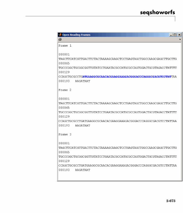
seqshoworfs
2-673

seqshoworfs
Identify the open reading frames in a GenBank sequence.
HLA_DQB1 = getgenbank('NM_002123');seqshoworfs(HLA_DQB1.Sequence);
See Also Bioinformatics Toolbox functions: codoncount, cpgisland,geneticcode, seqdisp, seqshowwords, seqtool, seqwordcount
MATLAB function: regexp
2-674
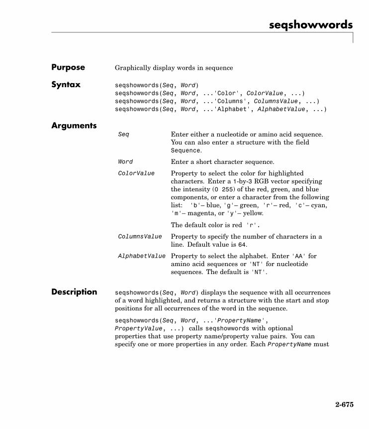
seqshowwords
Purpose Graphically display words in sequence
Syntax seqshowwords(Seq, Word)seqshowwords(Seq, Word, ...'Color', ColorValue, ...)seqshowwords(Seq, Word, ...'Columns', ColumnsValue, ...)seqshowwords(Seq, Word, ...'Alphabet', AlphabetValue, ...)
ArgumentsSeq Enter either a nucleotide or amino acid sequence.
You can also enter a structure with the fieldSequence.
Word Enter a short character sequence.
ColorValue Property to select the color for highlightedcharacters. Enter a 1-by-3 RGB vector specifyingthe intensity (0 255) of the red, green, and bluecomponents, or enter a character from the followinglist: 'b'– blue, 'g'– green, 'r'– red, 'c'– cyan,'m'– magenta, or 'y'– yellow.
The default color is red 'r'.
ColumnsValue Property to specify the number of characters in aline. Default value is 64.
AlphabetValue Property to select the alphabet. Enter 'AA' foramino acid sequences or 'NT' for nucleotidesequences. The default is 'NT'.
Description seqshowwords(Seq, Word) displays the sequence with all occurrencesof a word highlighted, and returns a structure with the start and stoppositions for all occurrences of the word in the sequence.
seqshowwords(Seq, Word, ...'PropertyName',PropertyValue, ...) calls seqshowwords with optionalproperties that use property name/property value pairs. You canspecify one or more properties in any order. Each PropertyName must
2-675
seqshowwords
be enclosed in single quotes and is case insensitive. These propertyname/property value pairs are as follows:
seqshowwords(Seq, Word, ...'Color', ColorValue, ...) selectsthe color used to highlight the words in the output display.
seqshowwords(Seq, Word, ...'Columns', ColumnsValue, ...)specifies how many columns per line to use in the output.
seqshowwords(Seq, Word, ...'Alphabet', AlphabetValue, ...)selects the alphabet for the sequence (Seq) and the word (Word).
If the search work (Word) contains nucleotide or amino acid symbolsthat represent multiple possible symbols, then seqshowwords shows allmatches. For example, the symbol R represents either G or A (purines).If Word is 'ART', then seqshowwords shows occurrences of both 'AAT'and 'AGT'.
Examples This example shows two matches, 'TAGT' and 'TAAT', for the word'BART'.
seqshowwords('GCTAGTAACGTATATATAAT','BART')
ans =Start: [3 17]Stop: [6 20]
000001 GCTAGTAACGTATATATAAT
seqshowwords does not highlight overlapping patterns multiple times.This example highlights two places, the first occurrence of 'TATA'and the 'TATATATA' immediately after 'CG'. The final 'TA' is nothighlighted because the preceding 'TA' is part of an already matchedpattern.
seqshowwords('GCTATAACGTATATATATA','TATA')
ans =Start: [3 10 14]
2-676

seqshowwords
Stop: [6 13 17]
000001 GCTATAACGTATATATATA
To highlight all multiple repeats of TA, use the regular expression'TA(TA)*TA'.
seqshowwords('GCTATAACGTATATATATA','TA(TA)*TA')
ans =Start: [3 10]Stop: [6 19]
000001 GCTATAACGTATATATATA
See Also Bioinformatics Toolbox functions: palindromes, cleave, restrict,seqdisp, seqtool, seqwordcount
MATLAB functions: strfind, regexp
2-677
seqtool
Purpose Open tool to interactively explore biological sequences
Syntax seqtool(Seq)seqtool(..., 'PropertyName', PropertyValue,...)seqtool(..., 'Alphabet', AlphabetValue)
ArgumentsSeq Struct with a field Sequence, a character array, or a file name
with an extension of .gbk, .gpt, .fasta, .fa, or .ebi
Description seqtool(Seq) loads a sequence (Seq) into the seqtool GUI.
seqtool(..., 'PropertyName', PropertyValue,...) definesoptional properties using property name/value pairs.
seqtool(..., 'Alphabet', AlphabetValue) specifies an alphabet(AlphabetValue) for the sequence (Seq). Default is 'AA', exceptwhen all of the symbols in the sequence are A, C, G, T, and -, thenAlphabetValue is set to 'NT'. Use 'AA' when you want to force anamino acid sequence alphabet.
Example 1 Get a sequence from Genbank.
S = getgenbank('M10051')
2 Open the sequence tool window with the sequence.
seqtool(S)
2-678

seqtool
See Also Bioinformatics Toolbox functions: aa2nt, aacount, aminolookup,basecount, baselookup, dimercount, emblread, fastaread,fastawrite, genbankread, geneticcode, genpeptread, getembl,getgenbank, getgenpept, nt2aa, proteinplot, seqcomplement,seqdisp, seqrcomplement, seqreverse, seqshoworfs, seqshowwords,seqwordcount
2-679
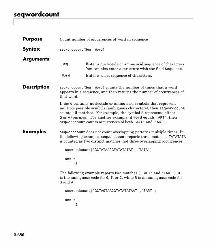
seqwordcount
Purpose Count number of occurrences of word in sequence
Syntax seqwordcount(Seq, Word)
ArgumentsSeq Enter a nucleotide or amino acid sequence of characters.
You can also enter a structure with the field Sequence.
Word Enter a short sequence of characters.
Description seqwordcount(Seq, Word) counts the number of times that a wordappears in a sequence, and then returns the number of occurrences ofthat word.
If Word contains nucleotide or amino acid symbols that representmultiple possible symbols (ambiguous characters), then seqwordcountcounts all matches. For example, the symbol R represents eitherG or A (purines). For another example, if word equals 'ART', thenseqwordcount counts occurrences of both 'AAT' and 'AGT'.
Examples seqwordcount does not count overlapping patterns multiple times. Inthe following example, seqwordcount reports three matches. TATATATAis counted as two distinct matches, not three overlapping occurrences.
seqwordcount('GCTATAACGTATATATAT','TATA')
ans =3
The following example reports two matches ('TAGT' and 'TAAT'). Bis the ambiguous code for G, T, or C, while R is an ambiguous code forG and A.
seqwordcount('GCTAGTAACGTATATATAAT','BART')
ans =2
2-680

seqwordcount
See Also Bioinformatics Toolbox functions codoncount, seqshoworfs,seqshowwords, seqtool, seq2regexp
MATLAB functions strfind
2-681

showalignment
Purpose Sequence alignment with color
Syntax showalignment(Alignment)showalignment(Alignment, ...'MatchColor',MatchColorValue, ...)showalignment(Alignment,...'SimilarColor' SimilarColorValue,
...)showalignment(Alignment, ...'StartPointers',
StartPointersValue, ...)showalignment(Alignment, ...'Columns', ColumnsValue, ...)
ArgumentsAlignment For pairwise alignments, matches and
similar residues are highlighted andAlignment is the output from one ofthe functions nwalign or swalign. Formultiple sequence alignment highlyconserved columns are highlighted andAlignment is the output from the functionmultialign.
MatchColorValue Property to select the color to highlightmatching characters. Enter a 1-by-N RGBvector specifying the intensity (0 to 255) ofthe red, green, and blue components, orenter a character from the following list:'b'– blue, 'g'– green, 'r'– red, 'c'–cyan, 'm'– magenta, or 'y'– yellow.
The default color is red, 'r'.
SimilarColorValue Property to select the color to highlightsimilar characters. Enter a 1-by-3 RGBvector or color character. The default coloris magenta.
2-682
showalignment
StarterPointersValue Property to specify the starting indices ofthe aligned sequences. StartPointers isthe two element vector returned as thethird output of the function swalign.
ColumnsValue Property to specify the number ofcharacters in a line. Enter the numberof characters to display in one row. Thedefault value is 64.
Description showalignment(Alignment) displays an alignment in a MATLABfigure window.
showalignment(Alignment, ...'PropertyName',PropertyValue, ...) calls showalignment with optionalproperties that use property name/property value pairs. You canspecify one or more properties in any order. Each PropertyName mustbe enclosed in single quotes and is case insensitive. These propertyname/property value pairs are as follows:
showalignment(Alignment, ...'MatchColor',MatchColorValue, ...) selects the color to highlight the matches inthe output display. The default color is red. For example, to use cyan,enter 'c' or [0 255 255].
showalignment(Alignment, ...'SimilarColor'SimilarColorValue, ...) selects the color to highlightsimilar residues that are not exact matches. The default color ismagenta.
The following options are only available when showing pairwisealignments:
showalignment(Alignment,...'StartPointers', StartPointersValue, ...) specifies thestarting indices in the original sequences of a local alignment.
showalignment(Alignment, ...'Columns', ColumnsValue, ...)specifies how many columns per line to use in the output, and labels thestart of each row with the sequence positions.
2-683
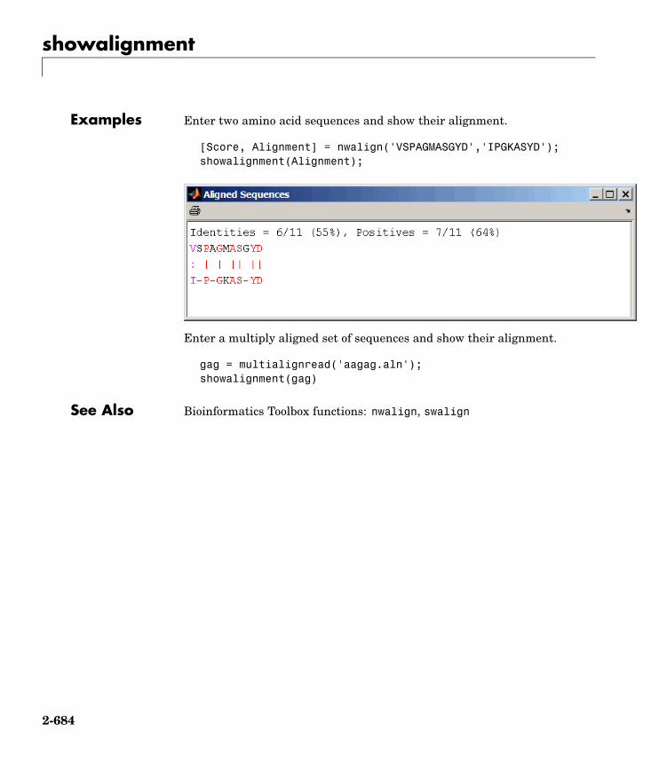
showalignment
Examples Enter two amino acid sequences and show their alignment.
[Score, Alignment] = nwalign('VSPAGMASGYD','IPGKASYD');showalignment(Alignment);
Enter a multiply aligned set of sequences and show their alignment.
gag = multialignread('aagag.aln');showalignment(gag)
See Also Bioinformatics Toolbox functions: nwalign, swalign
2-684

showhmmprof
Purpose Plot Hidden Markov Model (HMM) profile
Syntax showhmmprof(Model)showhmmprof(..., 'PropertyName', PropertyValue,...)showhmmprof(..., 'Scale', ScaleValue)showhmmprof(..., 'Order', OrderValue)
Arguments Model Hidden Markov model created by the functiongethmmprof or pfamhmmread.
ScaleValue Property to select a probability scale. Enter one of thefollowing values:• 'logprob' — Log probabilities
• 'prob' — Probabilities
• 'logodds' — Log-odd ratios
OrderValue Property to specify the order of the amino acidalphabet. Enter a character string with the 20standard amino acids characters A R N D C Q E G HI L K M F P S T W Y V. The ambiguous characters BZ X are not allowed.
Description showhmmprof(Model) plots a profile hidden Markov model described bythe structure Model.
showhmmprof(..., 'PropertyName', PropertyValue,...) definesoptional properties using property name/value pairs.
showhmmprof(..., 'Scale', ScaleValue) specifies the scale touse. If log probabilities (ScaleValue='logprob'), probabilities(ScaleValue='prob'), or log-odd ratios (ScaleValue='logodds'). Tocompute the log-odd ratios, the null model probabilities are used forsymbol emission and equally distributed transitions are used for thenull transition probabilities. The default ScaleValue is 'logprob'.
showhmmprof(..., 'Order', OrderValue) specifies the order inwhich the symbols are arranged along the vertical axis. This option
2-685

showhmmprof
allows you reorder the alphabet and group the symbols according totheir properties.
Examples 1 Load a model example.
model = pfamhmmread('pf00002.ls')
2 Plot the profile.
showhmmprof(model, 'Scale', 'logodds')
3 Order the alphabet by hydrophobicity.
hydrophobic = 'IVLFCMAGTSWYPHNDQEKR'
4 Plot the profile.
showhmmprof(model, 'Order', hydrophobic)
See Also Bioinformatics Toolbox functions: gethmmprof, hmmprofalign,hmmprofestimate, hmmprofgenerate, hmmprofstruct, pfamhmmread
2-686
sptread
Purpose Read data from SPOT file
Syntax SPOTData = sptread(File)SPOTData = sptread(File, 'CleanColNames',CleanColNamesValue)
ArgumentsFile Either of the following:
• String specifying a file name, a path andfile name, or a URL pointing to a file. Thereferenced file is a SPOT-formatted file(ASCII text file). If you specify only a filename, that file must be on the MATLABsearch path or in the MATLAB CurrentDirectory.
• MATLAB character array that contains thetext of a SPOT-formatted file.
CleanColNamesValue Property to control using valid MATLABvariable names.
Description SPOTData = sptread(File) reads a SPOT formatted file, File,) andcreates a MATLAB structure, SPOTData, containing the following fields:
HeaderDataBlocksColumnsRowsIDsColumnNamesIndicesShape
2-687

sptread
SPOTData = sptread(File, 'CleanColNames',CleanColNamesValue) The column names in the SPOT file containperiods and some characters that cannot be used in MATLAB variablenames. If you plan to use the column names as variable names in afunction, use this option with CleanColNames set to true and thefunction will return the field ColumnNames with valid variable names.
The Indices field of the structure includes the MATLAB indices thatyou can use for plotting heat maps of the data.
Examples 1 Read in a sample SPOT file and plot the median foreground intensityfor the 635 nm channel. Note that the example file spotdata.txtis not provided with Bioinformatics Toolbox.
spotStruct = sptread('spotdata.txt')maimage(spotStruct,'Rmedian');
2 Alternatively, create a similar plot using more basic graphicscommands.
Rmedian = magetfield(spotStruct,'Rmedian');imagesc(Rmedian(spotStruct.Indices));colormap bonecolorbar
See Also Bioinformatics Toolbox functions: affyread, agferead,celintensityread, geosoftread, gprread, imageneread, maboxplot,magetfield
2-688

svmclassify
Purpose Classify data using support vector machine
Syntax Group = svmclassify(SVMStruct, Sample)Group = svmclassify(SVMStruct, Sample, 'Showplot',ShowplotValue)
Description Group = svmclassify(SVMStruct, Sample) classifies each row of thedata in Sample using the information in a support vector machineclassifier structure SVMStruct, created using the svmtrain function.Sample must have the same number of columns as the data used totrain the classifier in svmtrain. Group indicates the group to whicheach row of Sample has been assigned.
Group = svmclassify(SVMStruct, Sample, 'Showplot',ShowplotValue) controls the plotting of the sample data in the figurecreated using the Showplot property with the svmtrain function.
Examples 1 Load the sample data, which includes Fisher’s iris data of 5measurements on a sample of 150 irises.
load fisheriris
2 Create data, a two-column matrix containing sepal length and sepalwidth measurements for 150 irises.
data = [meas(:,1), meas(:,2)];
3 From the species vector, create a new column vector, groups, toclassify data into two groups: Setosa and non-Setosa.
groups = ismember(species,'setosa');
4 Randomly select training and test sets.
[train, test] = crossvalind('holdOut',groups);cp = classperf(groups);
2-689

svmclassify
5 Use the svmtrain function to train an SVM classifier using a linearkernel function and plot the grouped data.
svmStruct = svmtrain(data(train,:),groups(train),'showplot',true);
6 Add a title to the plot, using the KernelFunction field from thesvmStruct structure as the title.
title(sprintf('Kernel Function: %s',...func2str(svmStruct.KernelFunction)),...'interpreter','none');
2-690
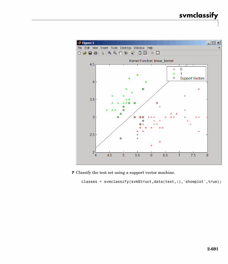
svmclassify
7 Classify the test set using a support vector machine.
classes = svmclassify(svmStruct,data(test,:),'showplot',true);
2-691
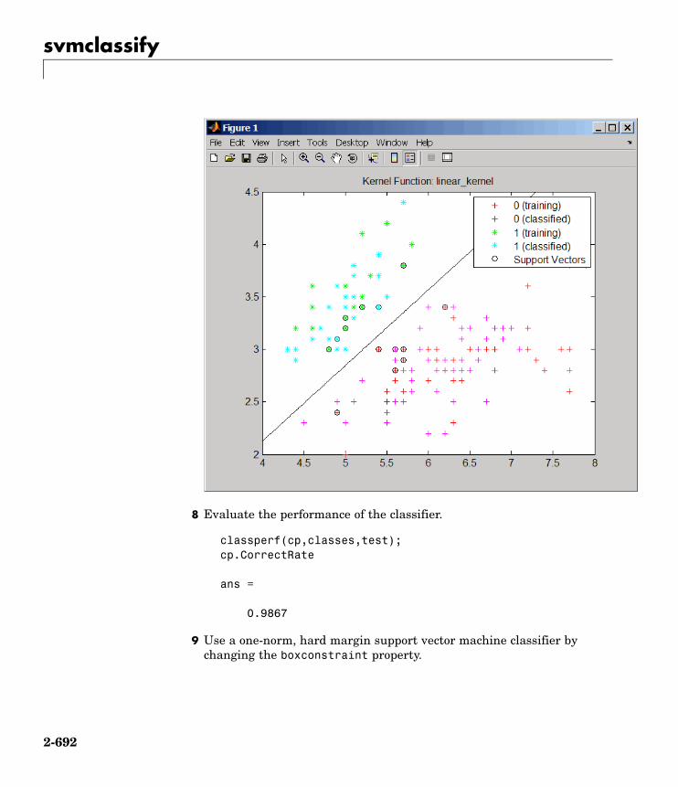
svmclassify
8 Evaluate the performance of the classifier.
classperf(cp,classes,test);cp.CorrectRate
ans =
0.9867
9 Use a one-norm, hard margin support vector machine classifier bychanging the boxconstraint property.
2-692

svmclassify
figuresvmStruct = svmtrain(data(train,:),groups(train),...
'showplot',true,'boxconstraint',1e6);
classes = svmclassify(svmStruct,data(test,:),'showplot',true);
2-693

svmclassify
10 Evaluate the performance of the classifier.
classperf(cp,classes,test);cp.CorrectRate
ans =
0.9867
2-694

svmclassify
References [1] Kecman, V., Learning and Soft Computing, MIT Press, Cambridge,MA. 2001.
[2] Suykens, J.A.K., Van Gestel, T., De Brabanter, J., De Moor, B.,and Vandewalle, J., Least Squares Support Vector Machines, WorldScientific, Singapore, 2002.
[3] Scholkopf, B., and Smola, A.J., Learning with Kernels, MIT Press,Cambridge, MA. 2002.
[4] Cristianini, N., and Shawe-Taylor, J. (2000). An Introductionto Support Vector Machines and Other Kernel-based LearningMethods, First Edition (Cambridge: Cambridge University Press).http://www.support-vector.net/
See Also Bioinformatics Toolbox functions: classperf, crossvalind,knnclassify, svmtrain
Statistics Toolbox function: classify
Optimization Toolbox function: quadprog
2-695

svmsmoset
Purpose Create or edit Sequential Minimal Optimization (SMO) optionsstructure
Syntax SMO_OptsStruct = svmsmoset('Property1Name', Property1Value,'Property2Name', Property2Value, ...)
SMO_OptsStruct = svmsmoset(OldOpts, 'Property1Name',Property1Value, 'Property2Name', Property2Value, ...)
SMO_OptsStruct = svmsmoset(OldOpts, NewOpts)
Arguments OldOpts Structure that specifies options used by the SMOmethod used by the svmtrain function.
NewOpts Structure that specifies options used by the SMOmethod used by the svmtrain function.
PropertyName Description of PropertyValue
TolKKT Value that specifies the tolerance with which theKKT conditions are checked. KKT conditionsare Karush-Kuhn-Tucker conditions. Default is1.0000e-003.
MaxIter Integer that specifies the maximum numberof iterations of the main loop. If this limitis exceeded before the algorithm converges,then the algorithm stops and returns an error.Default is 1500.
2-696

svmsmoset
PropertyName Description of PropertyValue
Display String that specifies the level of informationabout the optimization iterations that isdisplayed as the algorithm runs. Choices are:• off — Default. Reports nothing.
• iter — Reports every 10 iterations.
• final — Reports only when the algorithmfinishes.
KKTViolationLevel Value that specifies the fraction of variablesallowed to violate the KKT conditions. Choicesare any value ≥ 0 and < 1. Default is 0. Forexample, if you set KKTViolationLevel to 0.05,then 5% of the variables are allowed to violatethe KKT conditions.
Tip Set this option to a positive value to helpthe algorithm converge if it is fluctuating near agood solution.
For more information on KKT conditions, seeCristianini, et al. 2000.
KernelCacheLimit Value that specifies the size of the kernel matrixcache. The algorithm keeps a matrix with upto KernelCacheLimit × KernelCacheLimitdouble-precision, floating-point numbers inmemory. Default is 7500.
ReturnValues
SMO_OptsStruct Structure that specifies options used by the SMOmethod used by the svmtrain function.
2-697
svmsmoset
Description SMO_OptsStruct = svmsmoset('Property1Name', Property1Value,'Property2Name', Property2Value, ...) creates SMO_OptsStruct,an SMO options structure from the specified inputs. This structure canbe used as input for the svmtrain function.
SMO_OptsStruct = svmsmoset(OldOpts, 'Property1Name',Property1Value, 'Property2Name', Property2Value, ...) altersthe options in OldOpts, an existing SMO options structure, with thespecified inputs, creating a new output options structure.
SMO_OptsStruct = svmsmoset(OldOpts, NewOpts) alters the optionsin OldOpts, an existing SMO options structure, with the optionsspecified in NewOpts, another SMO options structure, creating a newoutput options structure.
Examples 1 Create an SMO options structure and specify the Display, MaxIter,and KernelCacheLimit properties.
opts = svmsmoset('Display','final','MaxIter',200,...'KernelCacheLimit',1000)
opts =
Display: 'final'TolKKT: 1.0000e-003
MaxIter: 200KKTViolationLevel: 0KernelCacheLimit: 1000
2 Create an alternate SMO options structure from the previousstructure. Specify different Display and KKTViolationLevelproperties.
alt_opts = svmsmoset(opts,'Display','iter','KKTViolationLevel',.05)
alt_opts =
Display: 'iter'
2-698

svmsmoset
TolKKT: 1.0000e-003
MaxIter: 200
KKTViolationLevel: 0.0500
KernelCacheLimit: 1000
References [1] Cristianini, N., and Shawe-Taylor, J. (2000). An Introductionto Support Vector Machines and Other Kernel-based LearningMethods, First Edition (Cambridge: Cambridge University Press).http://www.support-vector.net/
[2] Platt, J.C. (1999). Sequential Minimal Optimization: A FastAlgorithm for Training Support Vector Machines. In Advances inKernel Methods - Support Vector Learning, B. Scholkopf, J.C. Burges,and A.J. Smola, eds. (Cambridge MA: MIT Press), pp. 185–208.
See Also Bioinformatics Toolbox functions: svmclassify, svmtrain
Optimization Toolbox functions: optimset
2-699

svmtrain
Purpose Train support vector machine classifier
Syntax SVMStruct = svmtrain(Training, Group)SVMStruct = svmtrain(..., 'Kernel_Function',Kernel_FunctionValue, ...)SVMStruct = svmtrain(..., 'RBF_Sigma', RBFSigmaValue, ...)SVMStruct = svmtrain(..., 'Polyorder', PolyorderValue, ...)SVMStruct = svmtrain(..., 'Mlp_Params',Mlp_ParamsValue, ...)SVMStruct = svmtrain(..., 'Method', MethodValue, ...)SVMStruct = svmtrain(..., 'QuadProg_Opts',
QuadProg_OptsValue, ...)SVMStruct = svmtrain(..., 'SMO_Opts', SMO_OptsValue, ...)SVMStruct = svmtrain(..., 'BoxConstraint',
BoxConstraintValue, ...)SVMStruct = svmtrain(..., 'Autoscale', AutoscaleValue, ...)SVMStruct = svmtrain(..., 'Showplot', ShowplotValue, ...)
Arguments Training Matrix of training data, where each rowcorresponds to an observation or replicate,and each column corresponds to a featureor variable.
Group Column vector, character array, or cell arrayof strings for classifying data in Traininginto two groups. It has the same numberof elements as there are rows in Training.Each element specifies the group to whichthe corresponding row in Training belongs.
2-700
svmtrain
Kernel_FunctionValue String or function handle specifying thekernel function that maps the training datainto kernel space. Choices are:• linear — Default. Linear kernel or dot
product.
• quadratic — Quadratic kernel.
• rbf — Gaussian Radial Basis Functionkernel with a default scaling factor,sigma, of 1.
• polynomial — Polynomial kernel with adefault order of 3.
• mlp — Multilayer Perceptron kernel withdefault scale and bias parameters of [1,-1].
• @functionname — Handle to a kernelfunction specified using @and thefunctionname. For example, @kfun, or ananonymous function.
RBFSigmaValue Positive number that specifies the scalingfactor, sigma, in the radial basis functionkernel. Default is 1.
PolyorderValue Positive number that specifies the order of apolynomial kernel. Default is 3.
Mlp_ParamsValue Two-element vector, [p1, p2], thatspecifies the scale and bias parameters ofthe multilayer perceptron (mlp) kernel. K =tanh(p1*U*V' + p2). p1 must be > 0, andp2 must be < 0. Default is [1, -1].
2-701
svmtrain
MethodValue String specifying the method to find theseparating hyperplane. Choices are:• QP — Quadratic Programming (requires
Optimization Toolbox). The classifier isa two-norm, soft-margin support vectormachine.
• SMO — Sequential Minimal Optimization.The classifier is a one-norm, soft-marginsupport vector machine.
• LS — Least-Squares.
If you installed Optimization Toolbox, theQP method is the default. Otherwise, theSMO method is the default.
QuadProg_OptsValue An options structure created by theoptimset function (Optimization Toolbox).This structure specifies options used bythe QP method. For more information oncreating this structure, see the optimsetand quadprog reference pages.
SMO_OptsValue An options structure created by thesvmsmoset function. This structure specifiesoptions used by the SMO method. For moreinformation on creating this structure, seethe svmsmoset function.
2-702

svmtrain
BoxConstraintValue Box constraints for the soft margin. Choicesare:• Strictly positive numeric scalar.
• Array of strictly positive values with thenumber of elements equal to the numberof rows in the Training matrix.
If BoxConstraintValue is a scalar, it isautomatically rescaled by N/(2*N1) for thedata points of group one and by N/(2*N2)for the data points of group two. N1 is thenumber of elements in group one, N2 is thenumber of elements in group two, and N =N1 + N2. This rescaling is done to take intoaccount unbalanced groups, that is caseswhere N1 and N2 have very different values.
If BoxConstraintValue is an array, theneach array element is taken as a boxconstraint for the data point with the sameindex.Default is a scalar value of 1.
AutoscaleValue Controls the shifting and scaling ofdata points before training. WhenAutoscaleValue is true, the columns ofthe input data matrix Training are shiftedto zero mean and scaled to unit variance.Default is false.
ShowplotValue Controls the display of a plot of the groupeddata, including the separating line for theclassifier, when using two-dimensional data.Choices are true or false (default).
2-703
svmtrain
ReturnValues
SVMStruct Structure containing information aboutthe trained SVM classifier, including thefollowing fields:• SupportVectors
• Alpha
• Bias
• KernelFunction
• KernelFunctionArgs
• GroupNames
• SupportVectorIndices
• ScaleData
• FigureHandles
Tip You can use SVMStruct as inputto the svmclassify function, to use forclassification.
Description SVMStruct = svmtrain(Training, Group) trains a support vectormachine (SVM) classifier using Training, a matrix of training datataken from two groups, specified by Group. svmtrain treats NaNs orempty strings in Group as missing values and ignores the correspondingrows of Training. Information about the trained SVM classifier isreturned in SVMStruct, a structure with the following fields.
• SupportVectors
• Alpha
• Bias
• KernelFunction
2-704
svmtrain
• KernelFunctionArgs
• GroupNames
• SupportVectorIndices
• ScaleData
• FigureHandles
SVMStruct = svmtrain(Training, Group, ...'PropertyName',PropertyValue, ...) calls svmtrain with optional properties thatuse property name/property value pairs. You can specify one or moreproperties in any order. Each PropertyName must be enclosed in singlequotation marks and is case insensitive. These property name/propertyvalue pairs are as follows:
SVMStruct = svmtrain(..., 'Kernel_Function',Kernel_FunctionValue, ...) specifies the kernel function(Kernel_FunctionValue) that maps the training data into kernel space.Kernel_FunctionValue can be one of the following strings or a functionhandle:
• linear — Default. Linear kernel or dot product.
• quadratic — Quadratic kernel.
• rbf — Gaussian Radial Basis Function kernel with a default scalingfactor, sigma, of 1.
• polynomial — Polynomial kernel with a default order of 3.
• mlp — Multilayer Perceptron kernel with default scale and biasparameters of [1, -1].
• @functionname — Handle to a kernel function specified using @andthe functionname. For example, @kfun, or an anonymous function.
A kernel function must be of the following form:
function K = kfun(U, V)
2-705

svmtrain
Input arguments U and V are matrices with m and n rows respectively.Return value K is an m-by-n matrix. If kfun is parameterized, youcan use anonymous functions to capture the problem-dependentparameters. For example, suppose that your kernel function is:
function K = kfun(U,V,P1,P2)K = tanh(P1*(U*V')+P2);
You can set values for P1 and P2 and then use an anonymous functionas follows:
@(U,V) kfun(U,V,P1,P2)
For more information on the types of functions that can be used askernel functions, see Cristianini and Shawe-Taylor, 2000.
SVMStruct = svmtrain(..., 'RBF_Sigma', RBFSigmaValue, ...)specifies the scaling factor, sigma, in the radial basis function kernel.RBFSigmaValue must be a positive number. Default is 1.
SVMStruct = svmtrain(..., 'Polyorder', PolyorderValue, ...)specifies the order of a polynomial kernel. PolyorderValue must bea positive number. Default is 3.
SVMStruct = svmtrain(..., 'Mlp_Params', Mlp_ParamsValue,...) specifies the scale and bias parameters of the multilayerperceptron (mlp) kernel as a two-element vector, [p1, p2]. K =tanh(p1*U*V' + p2), p1 > 0, and p2 < 0. p1 must be > 0, and p2must be < 0. Default is [1, -1].
SVMStruct = svmtrain(..., 'Method', MethodValue, ...)specifies the method to find the separating hyperplane. Choices are:
• QP — Quadratic Programming (requires Optimization Toolbox). Theclassifier is a two-norm, soft-margin support vector machine.
• SMO — Sequential Minimal Optimization. The classifier is aone-norm, soft-margin support vector machine.
• LS — Least-Squares.
2-706

svmtrain
If you installed Optimization Toolbox, the QP method is the default.Otherwise, the SMO method is the default.
Note If you specify the QP method, the classifier is a two-norm,soft-margin support vector machine.
SVMStruct = svmtrain(..., 'QuadProg_Opts',QuadProg_OptsValue, ...) specifies an options structurecreated by the optimset function (Optimization Toolbox). This structurespecifies options used by the QP method. For more information oncreating this structure, see the optimset and quadprog functions.
SVMStruct = svmtrain(..., 'SMO_Opts', SMO_OptsValue, ...)specifies an options structure created by svmsmoset function. Thisstructure specifies options used by the SMO method. For moreinformation on creating this structure, see the svmsmoset function.
SVMStruct = svmtrain(..., 'BoxConstraint',BoxConstraintValue, ...) specifies box constraints for thesoft margin. BoxConstraintValue can be either of the following:
• Strictly positive numeric scalar
• Array of strictly positive values with the number of elements equal tothe number of rows in the Training matrix
If BoxConstraintValue is a scalar, it is automatically rescaled byN/(2*N1) for the data points of group one and by N/(2*N2) for the datapoints of group two. N1 is the number of elements in group one, N2 isthe number of elements in group two, and N = N1 + N2. This rescalingis done to take into account unbalanced groups, that is cases where N1and N2 have very different values.
If BoxConstraintValue is an array, then each array element is taken asa box constraint for the data point with the same index.
2-707

svmtrain
Default is a scalar value of 1.
SVMStruct = svmtrain(..., 'Autoscale', AutoscaleValue, ...)controls the shifting and scaling of data points before training. WhenAutoscaleValue is true, the columns of the input data matrix Trainingare shifted to zero mean and scaled to unit variance. Default is false.
SVMStruct = svmtrain(..., 'Showplot', ShowplotValue, ...),controls the display of a plot of the grouped data , including theseparating line for the classifier, when using two-dimensional data.Choices are true or false (default).
Memory Usage and Out of Memory Error
When you set 'Method' to 'QP', the svmtrain function operates on adata set containing N elements, it creates an (N+1)-by-(N+1) matrix tofind the separating hyperplane. This matrix needs at least 8*(n+1)^2bytes of contiguous memory. If this size of contiguous memory is notavailable, MATLAB displays an “out of memory” message.
When you set 'Method' to 'SMO', memory consumption is controlledby the SMO option KernelCacheLimit. For more information on theKernelCacheLimit option, see the svmsmoset function. The SMOalgorithm stores only a submatrix of the kernel matrix, limited by thesize specified by the KernelCacheLimit option. However, if the numberof data points exceeds the size specified by the KernelCacheLimitoption, the SMO algorithm slows down because it has to recalculatethe kernel matrix elements.
When using svmtrain on large data sets, and you run out of memory orthe optimization step is very time consuming, try either of the following:
• Use a smaller number of samples and use cross validation to testthe performance of the classifier.
• Set 'Method' to 'SMO', and set the KernelCacheLimit optionas large as your system permits. For information on setting theKernelCacheLimit option, see the svmsmoset function.
2-708

svmtrain
Tip If you set 'Method' to 'SMO', setting the 'BoxConstraint'property as small as possible will help the SMO algorithm run faster.
Examples 1 Load the sample data, which includes Fisher’s iris data of 5measurements on a sample of 150 irises.
load fisheriris
2 Create data, a two-column matrix containing sepal length and sepalwidth measurements for 150 irises.
data = [meas(:,1), meas(:,2)];
3 From the species vector, create a new column vector, groups, toclassify data into two groups: Setosa and non-Setosa.
groups = ismember(species,'setosa');
4 Randomly select training and test sets.
[train, test] = crossvalind('holdOut',groups);cp = classperf(groups);
5 Train an SVM classifier using a linear kernel function and plot thegrouped data.
svmStruct = svmtrain(data(train,:),groups(train),'showplot',true);
2-709
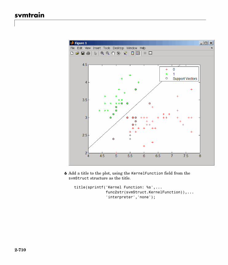
svmtrain
6 Add a title to the plot, using the KernelFunction field from thesvmStruct structure as the title.
title(sprintf('Kernel Function: %s',...func2str(svmStruct.KernelFunction)),...'interpreter','none');
2-710
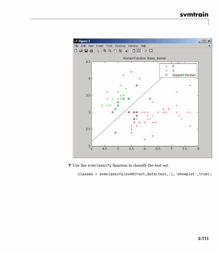
svmtrain
7 Use the svmclassify function to classify the test set.
classes = svmclassify(svmStruct,data(test,:),'showplot',true);
2-711

svmtrain
8 Evaluate the performance of the classifier.
classperf(cp,classes,test);cp.CorrectRate
ans =
0.9867
9 Use a one-norm, hard margin support vector machine classifier bychanging the boxconstraint property.
2-712

svmtrain
figuresvmStruct = svmtrain(data(train,:),groups(train),...
'showplot',true,'boxconstraint',1e6);
classes = svmclassify(svmStruct,data(test,:),'showplot',true);
2-713
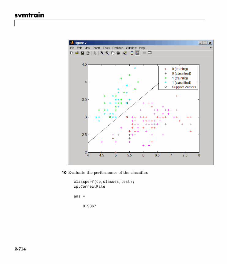
svmtrain
10 Evaluate the performance of the classifier.
classperf(cp,classes,test);cp.CorrectRate
ans =
0.9867
2-714

svmtrain
References [1] Kecman, V. (2001). Learning and Soft Computing (Cambridge, MA:MIT Press).
[2] Suykens, J.A.K., Van Gestel, T., De Brabanter, J., De Moor, B.,and Vandewalle, J. (2002). Least Squares Support Vector Machines(Singapore: World Scientific).
[3] Scholkopf, B., and Smola, A.J. (2002). Learning with Kernels(Cambridge, MA: MIT Press).
[4] Cristianini, N. and Shawe-Taylor, J. (2000). An Introductionto Support Vector Machines and Other Kernel-based LearningMethods, First Edition (Cambridge: Cambridge University Press).http://www.support-vector.net/
See Also Bioinformatics Toolbox functions: knnclassify, svmclassify,svmsmoset
Statistics Toolbox function: classify
Optimization Toolbox function: quadprog
MATLAB function: optimset
2-715

swalign
Purpose Locally align two sequences using Smith-Waterman algorithm
Syntax Score = swalign(Seq1, Seq2)[Score, Alignment] = swalign(Seq1, Seq2)[Score, Alignment, Start] = swalign(Seq1, Seq2)... = swalign(Seq1,Seq2, ...'Alphabet', AlphabetValue)... = swalign(Seq1,Seq2, ...'ScoringMatrix',
ScoringMatrixValue, ...)... = swalign(Seq1,Seq2, ...'Scale', ScaleValue, ...)... = swalign(Seq1,Seq2, ...'GapOpen', GapOpenValue, ...)... = swalign(Seq1,Seq2, ...'ExtendGap',ExtendGapValue, ...)... = swalign(Seq1,Seq2, ...'Showscore',ShowscoreValue, ...)
Arguments Seq1, Seq2 Amino acid or nucleotide sequences. Enterany of the following:• Character string of letters representing
amino acids or nucleotides, such as returnedby int2aa or int2nt
• Vector of integers representing amino acidsor nucleotides, such as returned by aa2intor nt2int
• Structure containing a Sequence field
Tip For help with letter and integerrepresentations of amino acids andnucleotides, see Amino Acid Lookup Table onpage 2-42 or Nucleotide Lookup Table on page2-52.
AlphabetValue String specifying the type of sequence. Choicesare 'AA' (default) or 'NT'.
2-716
swalign
ScoringMatrixValue String specifying the scoring matrix to use forthe local alignment. Choices for amino acidsequences are:
• 'PAM40'
• 'PAM250'
• 'DAYHOFF'
• 'GONNET'
• 'BLOSUM30' increasing by 5 up to'BLOSUM90'
• 'BLOSUM62'
• 'BLOSUM100'
Default is:
• 'BLOSUM50' (when AlphabetValue equals'AA')
• 'NUC44' (when AlphabetValue equals'NT')
Note All of the above scoring matrices have abuilt-in scale factor that returns Score in bits.
ScaleValue Scale factor used to return Score in arbitraryunits other than bits. Choices are any positivevalue. For example, if you enter log(2) forScaleValue, then swalign returns Score innats.
GapOpenValue Penalty for opening a gap in the alignment.Choices are any positive integer. Default is 8.
2-717

swalign
ExtendGapValue Penalty for extending a gap. Choices areany positive integer. Default is equal toGapOpenValue.
ShowscoreValue Controls the display of the scoring space andthe winning path of the alignment. Choicesare true or false (default).
ReturnValues
Score Optimal local alignment score in bits.
Alignment 3-by-N character array showing the twosequences, Seq1 and Seq2, in the first andthird rows, and symbols representing theoptimal local alignment between them in thesecond row.
Start 2-by-1 vector of indices indicating the startingpoint in each sequence for the alignment.
Description Score = swalign(Seq1, Seq2) returns the optimal local alignmentscore in bits. The scale factor used to calculate the score is provided bythe scoring matrix.
[Score, Alignment] = swalign(Seq1, Seq2) returns a 3-by-Ncharacter array showing the two sequences, Seq1 and Seq2, in the firstand third rows, and symbols representing the optimal local alignmentbetween them in the second row. The symbol | indicates amino acidsor nucleotides that match exactly. The symbol : indicates aminoacids or nucleotides that are related as defined by the scoring matrix(nonmatches with a zero or positive scoring matrix value).
[Score, Alignment, Start] = swalign(Seq1, Seq2) returns a2-by-1 vector of indices indicating the starting point in each sequencefor the alignment.
2-718
swalign
... = swalign(Seq1,Seq2, ...'PropertyName', PropertyValue,
...) calls swalign with optional properties that use propertyname/property value pairs. You can specify one or more properties inany order. Each PropertyName must be enclosed in single quotationmarks and is case insensitive. These property name/property valuepairs are as follows:
... = swalign(Seq1,Seq2, ...'Alphabet', AlphabetValue)specifies the type of sequences. Choices are 'AA' (default) or 'NT'.
... = swalign(Seq1,Seq2, ...'ScoringMatrix',ScoringMatrixValue, ...) specifies the scoring matrix to use for thelocal alignment. Default is:
• 'BLOSUM50' (when AlphabetValue equals 'AA')
• 'NUC44' (when AlphabetValue equals 'NT')
... = swalign(Seq1,Seq2, ...'Scale', ScaleValue, ...)specifies the scale factor used to return Score in arbitrary units otherthan bits. Choices are any positive value.
... = swalign(Seq1,Seq2, ...'GapOpen', GapOpenValue, ...)specifies the penalty for opening a gap in the alignment. Choices areany positive integer. Default is 8.
... = swalign(Seq1,Seq2, ...'ExtendGap', ExtendGapValue,
...) specifies the penalty for extending a gap in the alignment. Choicesare any positive integer. Default is equal to GapOpenValue.
... = swalign(Seq1,Seq2, ...'Showscore', ShowscoreValue,
...) controls the display of the scoring space and winning path of thealignment. Choices are true or false (default)
2-719

swalign
The scoring space is a heat map displaying the best scores for allthe partial alignments of two sequences. The color of each (n1,n2)coordinate in the scoring space represents the best score for the pairingof subsequences Seq1(s1:n1) and Seq2(s2:n2), where n1 is a positionin Seq1, n2 is a position in Seq2, s1 is any position in Seq1 between1:n1, and s2 is any position in Seq2 between 1:n2. The best score for apairing of specific subsequences is determined by scoring all possiblealignments of the subsequences by summing matches and gap penalties.
2-720
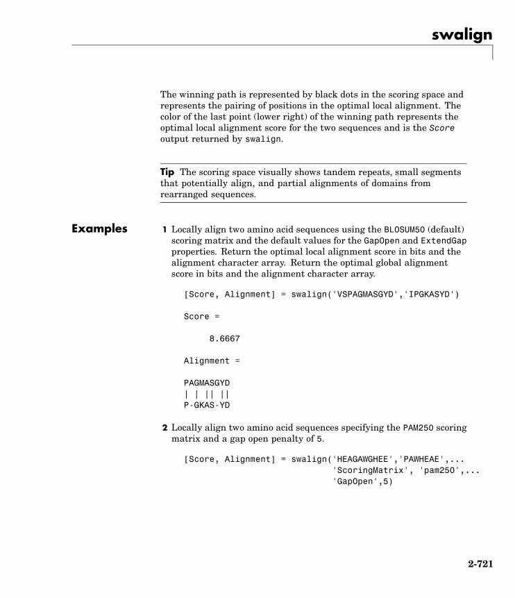
swalign
The winning path is represented by black dots in the scoring space andrepresents the pairing of positions in the optimal local alignment. Thecolor of the last point (lower right) of the winning path represents theoptimal local alignment score for the two sequences and is the Scoreoutput returned by swalign.
Tip The scoring space visually shows tandem repeats, small segmentsthat potentially align, and partial alignments of domains fromrearranged sequences.
Examples 1 Locally align two amino acid sequences using the BLOSUM50 (default)scoring matrix and the default values for the GapOpen and ExtendGapproperties. Return the optimal local alignment score in bits and thealignment character array. Return the optimal global alignmentscore in bits and the alignment character array.
[Score, Alignment] = swalign('VSPAGMASGYD','IPGKASYD')
Score =
8.6667
Alignment =
PAGMASGYD| | || ||P-GKAS-YD
2 Locally align two amino acid sequences specifying the PAM250 scoringmatrix and a gap open penalty of 5.
[Score, Alignment] = swalign('HEAGAWGHEE','PAWHEAE',...'ScoringMatrix', 'pam250',...'GapOpen',5)
2-721

swalign
Score =
8Alignment =
GAWGHE:|| ||PAW-HE
3 Locally align two amino acid sequences returning the Score in natunits (nats) by specifying a scale factor of log(2).
[Score, Alignment] = swalign('HEAGAWGHEE','PAWHEAE','Scale',log(2))
Score =
6.4694
Alignment =
AWGHE
|| ||
AW-HE
References [1] Durbin, R., Eddy, S., Krogh, A., and Mitchison, G. (1998). BiologicalSequence Analysis (Cambridge University Press).
[2] Smith, T., and Waterman, M. (1981). Identification of commonmolecular subsequences. Journal of Molecular Biology 147, 195–197.
See Also Bioinformatics Toolbox functions: blosum, nt2aa, nwalign, pam,seqdotplot, showalignment
2-722

traceplot
Purpose Draw nucleotide trace plots
Syntax traceplot(TraceStructure)traceplot(A, C, G, T)h = traceplot()
Description traceplot(TraceStructure) creates a trace plot from data in astructure with fields A, C, G, T.
traceplot(A, C, G, T) creates a trace plot from data in vectors A,C, G, T.
h = traceplot() returns a structure with the handles of the linescorresponding to A, C, G, T.
Examples tstruct = scfread('sample.scf');traceplot(tstruct)
See Also Bioinformatics Toolbox
• function — scfread
2-723


3
Methods — By Category
Phylogenetic Tree (p. 3-1) Select, modify, and plot phylogenetictrees using phytree object methods
Graph Visualization (p. 3-2) View relationships between datavisually with interactive maps,hierarchy plots, and pathways usingbiograph object methods
Gene Ontology (p. 3-3) Explore and analyze Gene Ontologydata using geneont object methods
Phylogenetic TreeFollowing are methods for use with a phytree object.
get (phytree) Information about phylogenetic treeobject
getbyname (phytree) Branches and leaves from phytreeobject
getcanonical (phytree) Calculate canonical form ofphylogenetic tree
getmatrix (phytree) Convert phytree object intorelationship matrix
getnewickstr (phytree) Create Newick-formatted string
pdist (phytree) Calculate pair-wise patristicdistances in phytree object
3 Methods — By Category
plot (phytree) Draw phylogenetic tree
prune (phytree) Remove branch nodes fromphylogenetic tree
reorder (phytree) Reorder leaves of phylogenetic tree
reroot (phytree) Change root of phylogenetic tree
select (phytree) Select tree branches and leaves inphytree object
subtree (phytree) Extract phylogenetic subtree
view (phytree) View phylogenetic tree
weights (phytree) Calculate weights for phylogenetictree
Graph VisualizationFollowing are methods for use with a biograph object.
allshortestpaths (biograph) Find all shortest paths in biographobject
conncomp (biograph) Find strongly or weakly connectedcomponents in biograph object
dolayout (biograph) Calculate node positions and edgetrajectories
getancestors (biograph) Find ancestors in biograph object
getdescendants (biograph) Find descendants in biograph object
getedgesbynodeid (biograph) Get handles to edges in biographobject
getmatrix (biograph) Get connection matrix from biographobject
getnodesbyid (biograph) Get handles to nodes
getrelatives (biograph) Find relatives in biograph object
3-2
Gene Ontology
isdag (biograph) Test for cycles in biograph object
isomorphism (biograph) Find isomorphism between twobiograph objects
isspantree (biograph) Determine if tree created frombiograph object is spanning tree
maxflow (biograph) Calculate maximum flow andminimum cut in biograph object
minspantree (biograph) Find minimal spanning tree inbiograph object
shortestpath (biograph) Solve shortest path problem inbiograph object
topoorder (biograph) Perform topological sort of directedacyclic graph extracted frombiograph object
traverse (biograph) Traverse biograph object by followingadjacent nodes
view (biograph) Draw figure from biograph object
Gene OntologyFollowing are methods for use with a geneont object.
getancestors (geneont) Numeric IDs for ancestors of GeneOntology term
getdescendants (geneont) Numeric IDs for descendants ofGene Ontology term
getmatrix (geneont) Convert geneont object intorelationship matrix
getrelatives (geneont) Numeric IDs for relatives of GeneOntology term
3-3

3 Methods — By Category
3-4

4
Methods — AlphabeticalList

allshortestpaths (biograph)
Purpose Find all shortest paths in biograph object
Syntax [dist] = allshortestpaths(BGObj)[dist] = allshortestpaths(BGObj, ...'Directed',DirectedValue, ...)[dist] = allshortestpaths(BGObj, ...'Weights', WeightsValue,
...)
ArgumentsBGObj biograph object created by biograph (object
constructor).
DirectedValue Property that indicates whether the graph is directedor undirected. Enter false for an undirected graph.This results in the upper triangle of the sparsematrix being ignored. Default is true.
WeightsValue Column vector that specifies custom weights for theedges in the N-by-N adjacency matrix extracted froma biograph object, BGObj. It must have one entry forevery nonzero value (edge) in the matrix. The orderof the custom weights in the vector must match theorder of the nonzero values in the matrix when it istraversed column-wise. This property lets you usezero-valued weights. By default, allshortestpathsgets weight information from the nonzero entries inthe matrix.
DescriptionTip For introductory information on graph theory functions, see “GraphTheory Functions” in the Bioinformatics Toolbox documentation.
[dist] = allshortestpaths(BGObj) finds the shortest paths betweenevery pair of nodes in a graph represented by an N-by-N adjacencymatrix extracted from a biograph object, BGObj, using Johnson’s
4-2

allshortestpaths (biograph)
algorithm. Nonzero entries in the matrix represent the weights of theedges.
Output dist is an N-by-N matrix where dist(S,T) is the distance ofthe shortest path from node S to node T. A 0 in this matrix indicates thesource node; an Inf is an unreachable node.
Johnson’s algorithm has a time complexity of O(N*log(N)+N*E), whereN and E are the number of nodes and edges respectively.
[...] = allshortestpaths (BGObj, 'PropertyName',PropertyValue, ...) calls allshortestpaths with optionalproperties that use property name/property value pairs. You canspecify one or more properties in any order. Each PropertyName mustbe enclosed in single quotes and is case insensitive. These propertyname/property value pairs are as follows:
[dist] = allshortestpaths(BGObj, ...'Directed',DirectedValue, ...) indicates whether the graph is directedor undirected. Set DirectedValue to false for an undirected graph.This results in the upper triangle of the sparse matrix being ignored.Default is true.
[dist] = allshortestpaths(BGObj, ...'Weights', WeightsValue, ...)lets you specify custom weights for the edges. WeightsValue is acolumn vector having one entry for every nonzero value (edge) in theN-by-N adjacency matrix extracted from a biograph object, BGObj. Theorder of the custom weights in the vector must match the order of thenonzero values in the N-by-N adjacency matrix when it is traversedcolumn-wise. This property lets you use zero-valued weights. Bydefault, allshortestpaths gets weight information from the nonzeroentries in the N-by-N adjacency matrix.
References [1] Johnson, D.B. (1977). Efficient algorithms for shortest paths insparse networks. Journal of the ACM 24(1), 1-13.
[2] Siek, J.G., Lee, L-Q, and Lumsdaine, A. (2002). The Boost GraphLibrary User Guide and Reference Manual, (Upper Saddle River,NJ:Pearson Education).
4-3

allshortestpaths (biograph)
See Also Bioinformatics Toolbox functions: biograph (object constructor),graphallshortestpaths
Bioinformatics Toolbox object: biograph object
Bioinformatics Toolbox methods of a biograph object: conncomp, isdag,isomorphism, isspantree, maxflow, minspantree, shortestpath,topoorder, traverse
4-4

conncomp (biograph)
Purpose Find strongly or weakly connected components in biograph object
Syntax [S, C] = conncomp(BGObj)[S, C] = conncomp(BGObj, ...'Directed', DirectedValue, ...)[S, C] = conncomp(BGObj, ...'Weak', WeakValue, ...)
ArgumentsBGObj biograph object created by biograph (object
constructor).
DirectedValue Property that indicates whether the graph isdirected or undirected. Enter false for anundirected graph. This results in the uppertriangle of the sparse matrix being ignored.Default is true. A DFS-based algorithm computesthe connected components. Time complexity isO(N+E), where N and E are number of nodes andedges respectively.
WeakValue Property that indicates whether to find weaklyconnected components or strongly connectedcomponents. A weakly connected componentis a maximal group of nodes that are mutuallyreachable by violating the edge directions. SetWeakValue to true to find weakly connectedcomponents. Default is false, which finds stronglyconnected components. The state of this parameterhas no effect on undirected graphs because weaklyand strongly connected components are the samein undirected graphs. Time complexity is O(N+E),where N and E are number of nodes and edgesrespectively.
DescriptionTip For introductory information on graph theory functions, see “GraphTheory Functions” in the Bioinformatics Toolbox documentation.
4-5

conncomp (biograph)
[S, C] = conncomp(BGObj) finds the strongly connected componentsof an N-by-N adjacency matrix extracted from a biograph object, BGObjusing Tarjan’s algorithm. A strongly connected component is a maximalgroup of nodes that are mutually reachable without violating the edgedirections. The N-by-N sparse matrix represents a directed graph; allnonzero entries in the matrix indicate the presence of an edge.
The number of components found is returned in S, and C is a vectorindicating to which component each node belongs.
Tarjan’s algorithm has a time complexity of O(N+E), where N and E arethe number of nodes and edges respectively.
[S, C] = conncomp(BGObj, ...'PropertyName',PropertyValue, ...) calls conncomp with optional properties thatuse property name/property value pairs. You can specify one or moreproperties in any order. Each PropertyName must be enclosed in singlequotes and is case insensitive. These property name/property valuepairs are as follows:
[S, C] = conncomp(BGObj, ...'Directed', DirectedValue, ...)indicates whether the graph is directed or undirected. SetdirectedValue to false for an undirected graph. This results in theupper triangle of the sparse matrix being ignored. Default is true.A DFS-based algorithm computes the connected components. Timecomplexity is O(N+E), where N and E are number of nodes and edgesrespectively.
[S, C] = conncomp(BGObj, ...'Weak', WeakValue, ...) indicateswhether to find weakly connected components or strongly connectedcomponents. A weakly connected component is a maximal group ofnodes that are mutually reachable by violating the edge directions.Set WeakValue to true to find weakly connected components. Defaultis false, which finds strongly connected components. The state of thisparameter has no effect on undirected graphs because weakly andstrongly connected components are the same in undirected graphs.Time complexity is O(N+E), where N and E are number of nodes andedges respectively.
4-6

conncomp (biograph)
Note By definition, a single node can be a strongly connectedcomponent.
Note A directed acyclic graph (DAG) cannot have any stronglyconnected components larger than one.
References [1] Tarjan, R.E., (1972). Depth first search and linear graph algorithms.SIAM Journal on Computing 1(2), 146–160.
[2] Sedgewick, R., (2002). Algorithms in C++, Part 5 Graph Algorithms(Addison-Wesley).
[3] Siek, J.G., Lee, L-Q, and Lumsdaine, A. (2002). The Boost GraphLibrary User Guide and Reference Manual, (Upper Saddle River,NJ:Pearson Education).
See Also Bioinformatics Toolbox functions: biograph (object constructor),graphconncomp
Bioinformatics Toolbox object: biograph object
Bioinformatics Toolbox methods of a biograph object:allshortestpaths, isdag, isomorphism, isspantree, maxflow,minspantree, shortestpath, topoorder, traverse
4-7
dolayout (biograph)
Purpose Calculate node positions and edge trajectories
Syntax dolayout(BGobj)dolayout(BGobj, 'Paths', PathsOnlyValue)
Arguments BGobj Biograph object created by the biograph function(object constructor).
PathsOnlyValue Controls the calculation of only the edge paths,leaving the nodes at their current positions.Choices are true or false (default).
Description dolayout(BGobj) calls the layout engine to calculate the optimalposition for each node so that its 2-D rendering is clean and uncluttered,and then calculates the best curves to represent the edges. The layoutengine uses the following properties of the biograph object:
• LayoutType — Specifies the layout engine as 'hierarchical','equilibrium', or 'radial'.
• LayoutScale — Rescales the sizes of the node before calling thelayout engine. This gives more space to the layout and reduces theoverlapping of nodes.
• NodeAutoSize — Controls precalculating the node size before callingthe layout engine. When NodeAutoSize is set to 'on', the layoutengine uses the node properties FontSize and Shape, and thebiograph object property LayoutScale to precalculate the actual sizeof each node. When NodeAutoSize is set to 'off', the layout engineuses the node property Size.
For more information on the above properties, see Properties ofa Biograph Object on page 5-4. For information on accessing andspecifying the above properties of a biograph object, see and .
4-8

dolayout (biograph)
dolayout(BGobj, 'Paths', PathsOnlyValue) controls the calculationof only the edge paths, leaving the nodes at their current positions.Choices are true or false (default).
Examples 1 Create a biograph object.
cm = [0 1 1 0 0;1 0 0 1 1;1 0 0 0 0;0 0 0 0 1;1 0 1 0 0];bg = biograph(cm)Biograph object with 5 nodes and 9 edges.bg.nodes(1).Position
ans =
[]
Nodes do not have a position yet.
2 Call the layout engine and render the graph.
dolayout(bg)bg.nodes(1).Position
ans =
112 224
view(bg)
3 Manually modify a node position and recalculate the paths only.
bg.nodes(1).Position = [150 150];dolayout(bg, 'Pathsonly', true)view(bg)
See Also Bioinformatics Toolbox function: biograph (object constructor)
Bioinformatics Toolbox object: biograph object
4-9

dolayout (biograph)
Bioinformatics Toolbox methods of a biograph object: dolayout,getancestors, getdescendants, getedgesbynodeid, getnodesbyid,getrelatives, view
MATLAB functions: get, set
4-10
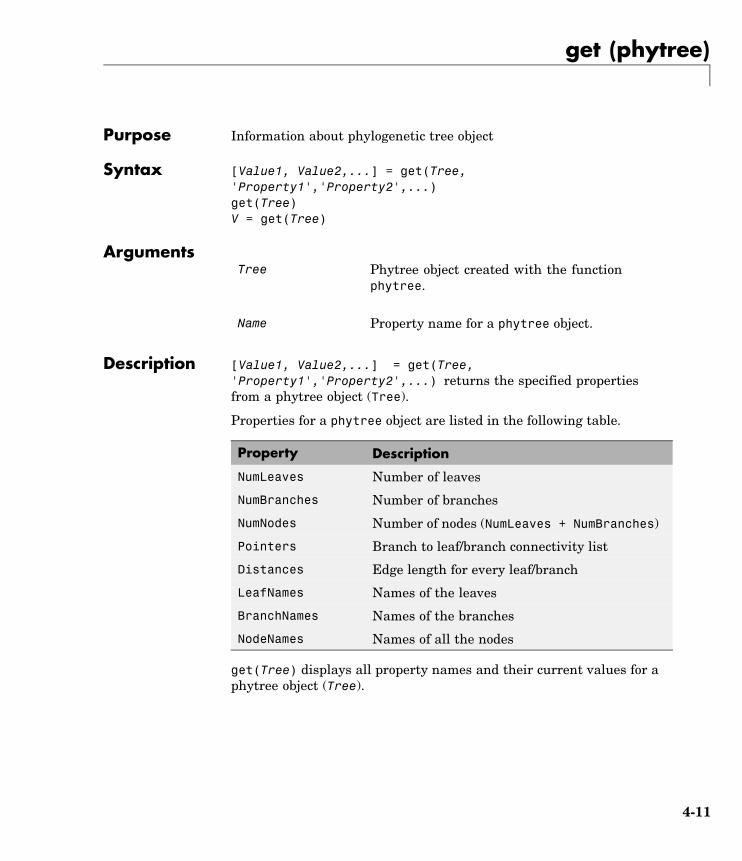
get (phytree)
Purpose Information about phylogenetic tree object
Syntax [Value1, Value2,...] = get(Tree,'Property1','Property2',...)get(Tree)V = get(Tree)
ArgumentsTree Phytree object created with the function
phytree.
Name Property name for a phytree object.
Description [Value1, Value2,...] = get(Tree,'Property1','Property2',...) returns the specified propertiesfrom a phytree object (Tree).
Properties for a phytree object are listed in the following table.
Property Description
NumLeaves Number of leaves
NumBranches Number of branches
NumNodes Number of nodes (NumLeaves + NumBranches)
Pointers Branch to leaf/branch connectivity list
Distances Edge length for every leaf/branch
LeafNames Names of the leaves
BranchNames Names of the branches
NodeNames Names of all the nodes
get(Tree) displays all property names and their current values for aphytree object (Tree).
4-11

get (phytree)
V = get(Tree) returns a structure where each field name is the nameof a property of a phytree object (Tree) and each field contains the valueof that property.
Examples 1 Read in a phylogenetic tree from a file.
tr = phytreeread('pf00002.tree')
2 Get the names of the leaves.
protein_names = get(tr,'LeafNames')
protein_names =
'BAI2_HUMAN/917-1197''BAI1_HUMAN/944-1191''O00406/622-883'...
See Also Bioinformatics Toolbox
• functions — phytree (object constructor), phytreeread
• phytree object methods — getbyname, select
4-12
getancestors (biograph)
Purpose Find ancestors in biograph object
Syntax Nodes = getancestors(BiographNode)Nodes = getancestors(BiographNode, NumGenerations)
ArgumentsBiographNode Node in a biograph object.
NumGenerations Number of generations. Enter a positiveinteger.
Description Nodes = getancestors(BiographNode) returns a node (BiographNode)and all of its direct ancestors.
Nodes = getancestors(BiographNode, NumGenerations) finds thenode (BiographNode) and its direct ancestors up to a specified numberof generations (NumGenerations).
Examples 1 Create a biograph object.
cm = [0 1 1 0 0;1 0 0 1 1;1 0 0 0 0;0 0 0 0 1;1 0 1 0 0];bg = biograph(cm)
2 Find one generation of ancestors for node 2.
ancNodes = getancestors(bg.nodes(2));set(ancNodes,'Color',[1 .7 .7]);bg.view;
4-13

getancestors (biograph)
3 Find two generations of ancestors for node 2.
ancNodes = getancestors(bg.nodes(2),2);set(ancNodes,'Color',[.7 1 .7]);bg.view;
4-14
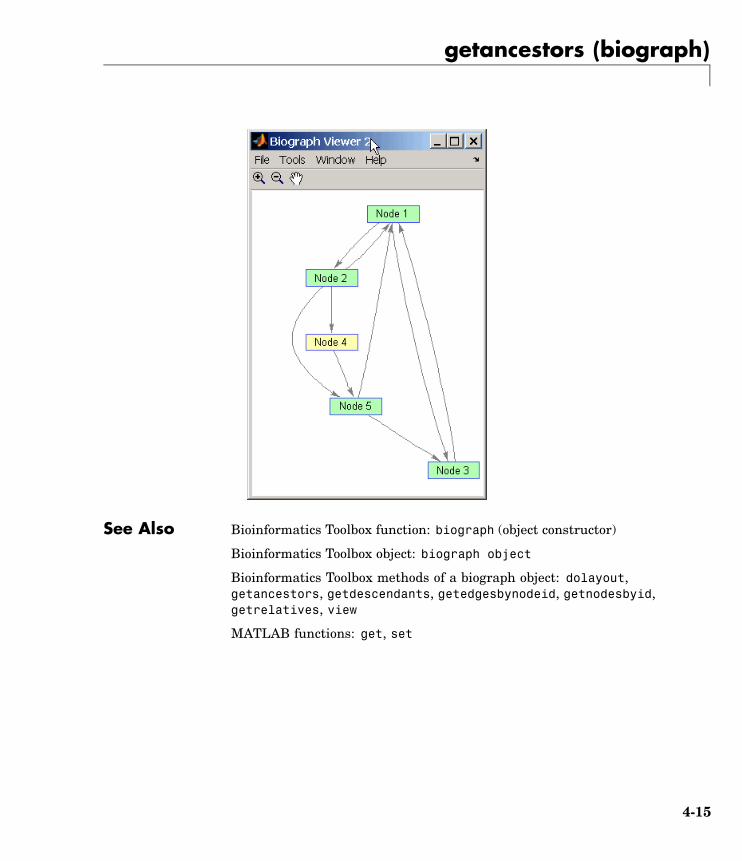
getancestors (biograph)
See Also Bioinformatics Toolbox function: biograph (object constructor)
Bioinformatics Toolbox object: biograph object
Bioinformatics Toolbox methods of a biograph object: dolayout,getancestors, getdescendants, getedgesbynodeid, getnodesbyid,getrelatives, view
MATLAB functions: get, set
4-15

getancestors (geneont)
Purpose Numeric IDs for ancestors of Gene Ontology term
Syntax AncestorIDs = getancestors(GeneontObj, ID)AncestorIDs = getancestors(..., 'Height', HeightValue, ...)
Description AncestorIDs = getancestors(GeneontObj, ID) returns the numericIDs (AncestorIDs) for the ancestors of a term (ID) including the ID forthe term. ID is a nonnegative integer or a numeric vector with a setof IDs.
AncestorIDs = getancestors(..., 'PropertyName',PropertyValue,...) defines optional properties using propertyname/value pairs.
AncestorIDs = getancestors(..., 'Height', HeightValue, ...)searches up through a specified number of levels (HeightValue) in theGene Ontology database. HeightValue is a positive integer. Defaultis Inf.
Examples 1 Download the Gene Ontology database from the Web into MATLAB.
GO = geneont('LIVE', true);
MATLAB creates a geneont object and displays the number of termsin the database.
Gene Ontology object with 20005 Terms.
2 Get the ancestors for a Gene Ontology term.
ancestors = getancestors(GO,46680)
ancestors =815096289636
1708542221
4-16

getancestors (geneont)
4668050896
3 Create a sub Gene Ontology.
subontology = GO(ancestors)
Gene Ontology object with 7 Terms.
4 View relationships using the biograph functions.
[cm acc rels] = getmatrix(subontology);BG = biograph(cm, get(subontology.Terms, 'name'))view(BG)
4-17
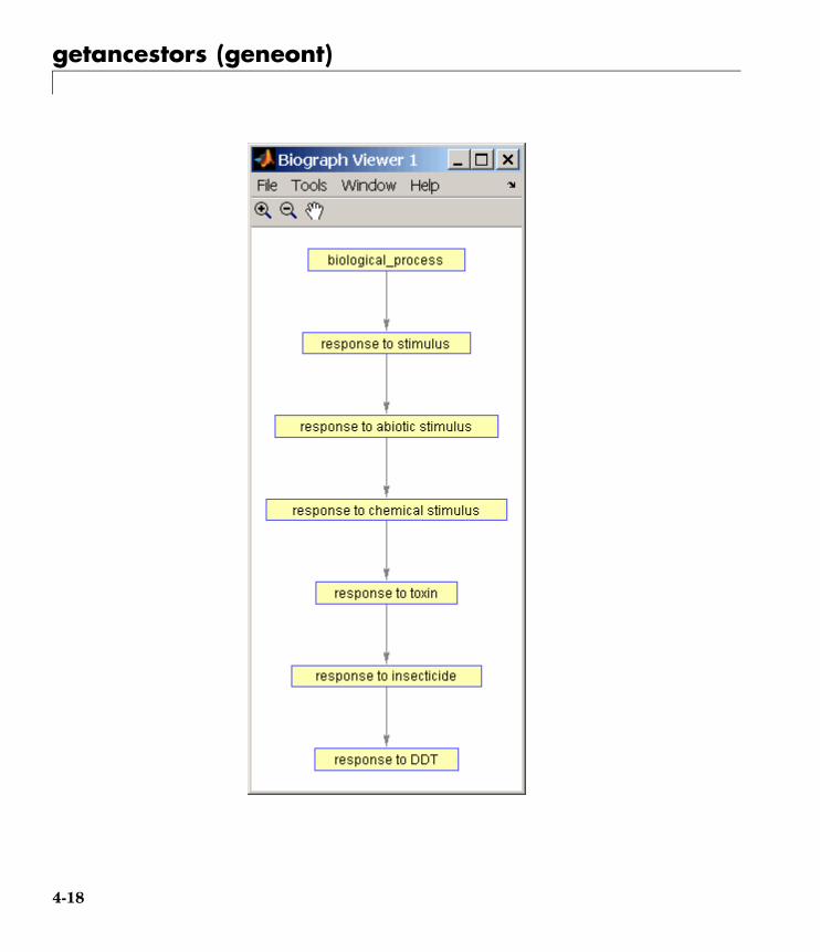
getancestors (geneont)
4-18

getancestors (geneont)
See Also Bioinformatics Toolbox
• functions — geneont (object constructor), goannotread, num2goid
• geneont object methods — getdescendants, getmatrix,getrelatives
4-19
getbyname (phytree)
Purpose Branches and leaves from phytree object
Syntax S = getbyname(Tree, Expression)S = getbyname(Tree, String, 'Exact', true)
ArgumentsTree phytree object created by phytree function (object
constructor).
Expression Regular expression. When Expression is a cellarray of strings, getbyname returns a matrixwhere every column corresponds to every query inExpression.
For information about the symbols that you can usein a matching regular expression, see the MATLABfunction regexp.
String String or cell array of strings.
Description S = getbyname(Tree, Expression) returns a logical vector (S) of sizeNumNodes-by-1 with the node names of a phylogenetic tree (Tree) thatmatch the regular expression (Expression) regardless of letter case.
S = getbyname(Tree, String, 'Exact', true) looks for exact stringmatches and ignores case. When String is a cell array of char strings,getbyname returns a vector with indices.
Examples 1 Load a phylogenetic tree created from a protein family.
tr = phytreeread('pf00002.tree');
2 Select all the ’mouse’ and ’human’ proteins.
sel = getbyname(tr,{'mouse','human'});view(tr,any(sel,2));
4-20

getbyname (phytree)
See Also Bioinformatics Toolbox
• function — phytree (object constructor)
• phytree object methods — get, prune, select
4-21
getcanonical (phytree)
Purpose Calculate canonical form of phylogenetic tree
Syntax Pointers = getcanonical(Tree)[Pointers, Distances, Names] = getcanonical(Tree)
ArgumentsTree phytree object created by phytree function
(object constructor).
Description Pointers = getcanonical(Tree) returns the pointers for thecanonical form of a phylogenetic tree (Tree). In a canonical tree theleaves are ordered alphabetically and the branches are ordered first bytheir width and then alphabetically by their first element. A canonicaltree is isomorphic to all the trees with the same skeleton independentlyof the order of their leaves and branches.
[Pointers, Distances, Names] = getcanonical(Tree) returns,in addition to the pointers described above, the reordered distances(Distances) and node names (Names).
Examples 1 Create two phylogenetic trees with the same skeleton but slightlydifferent distances.
b = [1 2; 3 4; 5 6; 7 8;9 10];tr_1 = phytree(b,[.1 .2 .3 .3 .4 ]');tr_2 = phytree(b,[.2 .1 .2 .3 .4 ]');
2 Plot the trees.
plot(tr_1)plot(tr_2)
3 Check whether the trees have an isomorphic construction.
isequal(getcanonical(tr_1),getcanonical(tr_2))
4-22
getcanonical (phytree)
ans =1
See Also Bioinformatics Toolbox
• functions — phytree (object constructor), phytreeread
• phytree object methods — getbyname, select, subtree
4-23

getdescendants (biograph)
Purpose Find descendants in biograph object
Syntax Nodes = getdescendants(BiographNode)Nodes = getdescendants(BiographNode,NumGenerations)
ArgumentsBiographNode Node in a biograph object.
NumGenerations Number of generations. Enter a positive integer.
Description Nodes = getdescendants(BiographNode) finds a given node(BiographNode) all of its direct descendants.
Nodes = getdescendants(BiographNode,NumGenerations) finds thenode (BiographNode) and all of its direct descendants up to a specifiednumber of generations (NumGenerations).
Examples 1 Create a biograph object.
cm = [0 1 1 0 0;1 0 0 1 1;1 0 0 0 0;0 0 0 0 1;1 0 1 0 0];bg = biograph(cm)
2 Find one generation of descendants for node 4.
desNodes = getdescendants(bg.nodes(4));set(desNodes,'Color',[1 .7 .7]);bg.view;
4-24
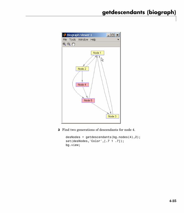
getdescendants (biograph)
3 Find two generations of descendants for node 4.
desNodes = getdescendants(bg.nodes(4),2);set(desNodes,'Color',[.7 1 .7]);bg.view;
4-25

getdescendants (biograph)
See Also Bioinformatics Toolbox function: biograph (object constructor)
Bioinformatics Toolbox object: biograph object
Bioinformatics Toolbox methods of a biograph object: dolayout,getancestors, getdescendants, getedgesbynodeid, getnodesbyid,getrelatives, view
MATLAB functions: get, set
4-26

getdescendants (geneont)
Purpose Numeric IDs for descendants of Gene Ontology term
Syntax DescendantIDs = getdescendants(GeneontObj, ID)DescendantIDs = getdescendants(..., 'Depth',DepthValue,...)
Description DescendantIDs = getdescendants(GeneontObj, ID)returns thenumeric IDs (DescendantIDs) for the descendants of a term (ID)including the ID for the term. ID is a nonnegative integer or a numericvector with a set of IDs.
DescendantIDs = getdescendants(..., 'PropertyName',PropertyValue,...) defines optional properties using propertyname/value pairs.
DescendantIDs = getdescendants(..., 'Depth',DepthValue,...) searches down through a specified numberof levels (DepthValue) in the Gene Ontology. DepthValue is a positiveinteger. Default is Inf.
Examples 1 Download the Gene Ontology database from the Web into MATLAB.
GO = geneont('LIVE', true);
MATLAB creates a geneont object and displays the number of termsin the database.
Gene Ontology object with 20005 Terms.
2 Get the ancestors for a Gene Ontology term.
descendants = getdescendants(GO,5622, 'Depth', 5)
3 Create a sub Gene Ontology.
subontology = GO(descendants)
Gene Ontology object with 1071 Terms.
4-27

getdescendants (geneont)
See Also Bioinformatics Toolbox
• functions — geneont (object constructor), goannotread, num2goid
• geneont object methods — getancestors, getmatrix, getrelatives
4-28

getedgesbynodeid (biograph)
Purpose Get handles to edges in biograph object
Syntax Edges = getedgesbynodeid(BGobj,SourceIDs,SinkIDs)
ArgumentsBGobj Biograph object.
SourceIDs,SinkIDs
Enter a cell string, or an empty cell array (getsall edges).
Description Edges = getedgesbynodeid(BGobj,SourceIDs,SinkIDs) gets thehandles to the edges that connect the specified source nodes (SourceIDs)to the specified sink nodes (SinkIDs) in a biograph object.
Example 1 Create a biograph object for the Hominidae family.
species = {'Homo','Pan','Gorilla','Pongo','Baboon',...'Macaca','Gibbon'};
cm = magic(7)>25 & 1-eye(7);bg = biograph(cm, species);
2 Find all the edges that connect to the Homo node.
EdgesIn = getedgesbynodeid(bg,[],'Homo');EdgesOut = getedgesbynodeid(bg,'Homo',[]);set(EdgesIn,'LineColor',[0 1 0]);set(EdgesOut,'LineColor',[1 0 0]);bg.view;
3 Find all edges that connect members of the Cercopithecidae family tomembers of the Hominidae family.
Cercopithecidae = {'Macaca','Baboon'};Hominidae = {'Homo','Pan','Gorilla','Pongo'};edgesSel = getedgesbynodeid(bg,Cercopithecidae,Hominidae);set(bg.edges,'LineColor',[.5 .5 .5]);set(edgesSel,'LineColor',[0 0 1]);
4-29

getedgesbynodeid (biograph)
bg.view;
See Also Bioinformatics Toolbox function: biograph (object constructor)
Bioinformatics Toolbox object: biograph object
Bioinformatics Toolbox methods of a biograph object: dolayout,getancestors, getdescendants, getedgesbynodeid, getnodesbyid,getrelatives, view
MATLAB functions: get, set
4-30

getmatrix (biograph)
Purpose Get connection matrix from biograph object
Syntax [Matrix, ID, Distances] = getmatrix(BGObj)
ArgumentsBGObj biograph object created by biograph (object
constructor).
Description [Matrix, ID, Distances] = getmatrix(BGObj) converts thebiograph object, BiographObj, into a logical sparse matrix, Matrix, inwhich 1 indicates that a node (row index) is connected to another node(column index). ID is a cell array of strings listing the ID propertiesfor each node, and corresponds to the rows and columns of Matrix.Distances is a column vector with one entry for every nonzero entry inMatrix traversed column-wise and representing the respective Weightproperty for each edge.
Examples cm = [0 1 1 0 0;2 0 0 4 4;4 0 0 0 0;0 0 0 0 2;4 0 5 0 0];bg = biograph(cm);[cm, IDs, dist] = getmatrix(bg)
See Also Bioinformatics Toolbox function: biograph (object constructor)
Bioinformatics Toolbox object: biograph object
Bioinformatics Toolbox methods of a biograph object: dolayout,getancestors, getdescendants, getedgesbynodeid, getnodesbyid,getrelatives, view
4-31

getmatrix (geneont)
Purpose Convert geneont object into relationship matrix
Syntax [Matrix, ID, Relationship] = getmatrix(GeneontObj)
ArgumentsGeneontObj geneont object created by geneont (object constructor)
Description [Matrix, ID, Relationship] = getmatrix(GeneontObj) convertsa geneont object, GeneontObj, into Matrix, a matrix of relationshipvalues between nodes (row and column indices), in which 0 indicatesno relationship, 1 indicates an “is_a” relationship, and 2 indicates a“part_of” relationship. ID is a column vector listing Gene Ontology IDsthat correspond to the rows and columns of Matrix. Relationship is acell array of strings defining the types of relationships.
Examples GO = geneont('LIVE',true);[MATRIX, ID, REL] = getmatrix(GO);
See Also • Bioinformatics Toolbox functions — geneont (object constructor),goannotread, num2goid
• Bioinformatics Toolbox object — geneont object
• Bioinformatics Toolbox methods of geneont object — getancestors,getdescendants, getmatrix, getrelatives
4-32

getmatrix (phytree)
Purpose Convert phytree object into relationship matrix
Syntax [Matrix, ID, Distances] = getmatrix(PhytreeObj)
ArgumentsPhytreeObj phytree object created by phytree (object constructor).
Description [Matrix, ID, Distances] = getmatrix(PhytreeObj) converts aphytree object, PhytreeObj, into a logical sparse matrix, Matrix, inwhich 1 indicates that a branch node (row index) is connected to itschild (column index). The child can be either another branch node ora leaf node. ID is a column vector of strings listing the labels thatcorrespond to the rows and columns of Matrix, with the labels from 1 toNumber of Leaves being the leaf nodes, then the labels from Numberof Leaves + 1 to Number of Leaves + Number of Branches being thebranch nodes, and the label for the last branch node also being the rootnode. Distances is a column vector with one entry for every nonzeroentry in Matrix traversed column-wise and representing the distancebetween the branch node and the child.
Examples T = phytreeread('pf00002.tree')[MATRIX, ID, DIST] = getmatrix(T);
See Also Bioinformatics Toolbox functions: phytree (object constructor),phytreetool
Bioinformatics Toolbox object: phytree object
Bioinformatics Toolbox methods of phytree object: get, pdist, prune
4-33
getnewickstr (phytree)
Purpose Create Newick-formatted string
Syntax String = getnewickstr(Tree)getnewickstr(..., 'PropertyName', PropertyValue,...)getnewickstr(..., 'Distances', DistancesValue)getnewickstr(..., 'BranchNames', BranchNamesValue)
ArgumentsTree Phytree object created with the function
phytree.
DistancesValue Property to control including or excludingdistances in the output. Enter either true(include distances) or false (exclude distances).Default is true.
BranchNamesValue Property to control including or excludingbranch names in the output. Enter either true(include branch names) or false (exclude branchnames). Default is false.
Description String = getnewickstr(Tree) returns the Newick formatted string ofa phylogenetic tree object (Tree).
getnewickstr(..., 'PropertyName', PropertyValue,...) definesoptional properties using property name/value pairs.
getnewickstr(..., 'Distances', DistancesValue), whenDistancesValue is false, excludes the distances from the output.
getnewickstr(..., 'BranchNames', BranchNamesValue), whenBranchNamesValue is true, includes the branch names in the output.
References Information about the Newick tree format.
http://evolution.genetics.washington.edu/phylip/newicktree.html
4-34

getnewickstr (phytree)
Examples 1 Create some random sequences.
seqs = int2nt(ceil(rand(10)*4));
2 Calculate pairwise distances.
dist = seqpdist(seqs,'alpha','nt');
3 Construct a phylogenetic tree.
tree = seqlinkage(dist);
4 Get the Newick string.
str = getnewickstr(tree)
See Also Bioinformatics Toolbox
• functions — phytree (object constructor), phytreeread,phytreetool, phytreewrite, seqlinkage
• phytree object methods — get, getbyname, getcanonical
4-35
getnodesbyid (biograph)
Purpose Get handles to nodes
Syntax NodesHandles = getnodesbyid(BGobj,NodeIDs)
ArgumentsBGobj Biograph object.
NodeIDs Enter a cell string of node identifications.
Description NodesHandles = getnodesbyid(BGobj,NodeIDs) gets the handles forthe specified nodes (NodeIDs) in a biograph object.
Example 1 Create a biograph object.
species = {'Homosapiens','Pan','Gorilla','Pongo','Baboon',...'Macaca','Gibbon'};
cm = magic(7)>25 & 1-eye(7);bg = biograph(cm, species)
2 Find the handles to members of the Cercopithecidae family andmembers of the Hominidae family.
Cercopithecidae = {'Macaca','Baboon'};Hominidae = {'Homosapiens','Pan','Gorilla','Pongo'};CercopithecidaeNodes = getnodesbyid(bg,Cercopithecidae);HominidaeNodes = getnodesbyid(bg,Hominidae);
3 Color the families differently and draw a graph.
See Also Bioinformatics Toolbox function: biograph (object constructor)
Bioinformatics Toolbox object: biograph object
Bioinformatics Toolbox methods of a biograph object: dolayout,getancestors, getdescendants, getedgesbynodeid, getnodesbyid,getrelatives, view
4-36

getnodesbyid (biograph)
MATLAB functions: get, set
4-37

getrelatives (biograph)
Purpose Find relatives in biograph object
Syntax Nodes = getrelatives(BiographNode)Nodes = getrelatives(BiographNode,NumGenerations)
ArgumentsBiographNode Node in a biograph object.
NumGenerations Number of generations. Enter a positiveinteger.
Description Nodes = getrelatives(BiographNode) finds all the direct relativesfor a given node (BiographNode).
Nodes = getrelatives(BiographNode,NumGenerations) finds thedirect relatives for a given node (BiographNode) up to a specifiednumber of generations (NumGenerations).
Examples 1 Create a biograph object.
cm = [0 1 1 0 0;1 0 0 1 1;1 0 0 0 0;0 0 0 0 1;1 0 1 0 0];bg = biograph(cm)
2 Find all nodes interacting with node 1.
intNodes = getrelatives(bg.nodes(1));set(intNodes,'Color',[.7 .7 1]);bg.view;
See Also Bioinformatics Toolbox function: biograph (object constructor)
Bioinformatics Toolbox object: biograph object
Bioinformatics Toolbox methods of a biograph object: dolayout,getancestors, getdescendants, getedgesbynodeid, getnodesbyid,getrelatives, view
MATLAB functions: get, set
4-38

getrelatives (geneont)
Purpose Numeric IDs for relatives of Gene Ontology term
Syntax RelativeIDs = getrelatives(GeneontObj, ID)getrelatives(..., 'PropertyName', PropertyValue,...)getrelatives(..., 'Height', HeightValue)getrelatives(..., 'Depth', DepthValue)
ArgumentsGeneontObj
ID
Description RelativeIDs = getrelatives(GeneontObj, ID) returns the numericIDs (RelativeIDs) for the relatives of a term (ID) including the ID forthe term. ID is a nonnegative integer or a numeric vector with a setof IDs.
getrelatives(..., 'PropertyName', PropertyValue,...) definesoptional properties using property name/value pairs.
getrelatives(..., 'Height', HeightValue) includes terms that arerelated up through a specified number of levels (HeightValue) in theGene Ontology database. HeightValue is a positive integer. Default is 1.
getrelatives(..., 'Depth', DepthValue) includes terms that arerelated down through a specified number of levels (DepthValue) in theGene Ontology database. DepthValue is a positive integer. Default is 1.
Examples 1 Download the Gene Ontology database from the Web into MATLAB.
GO = geneont('LIVE', true);
MATLAB creates a geneont object and displays the number of termsin the database.
Gene Ontology object with 20005 Terms.
2 Get the relatives for a Gene Ontology term.
4-39

getrelatives (geneont)
subontology = getrelatives(GO,46680)
See Also Bioinformatics Toolbox
• functions — geneont (object constructor), goannotread, num2goid
• geneont object methods — getancestors, getdescendants,getmatrix
4-40
isdag (biograph)
Purpose Test for cycles in biograph object
Syntax isdag(BGObj)
ArgumentsBGObj biograph object created by biograph (object constructor).
DescriptionTip For introductory information on graph theory functions, see “GraphTheory Functions” in the Bioinformatics Toolbox documentation.
isdag(BGObj) returns logical 1 (true) if an N-by-N adjacency matrixextracted from a biograph object, BGObj, is a directed acyclic graph(DAG) and logical 0 (false) otherwise. In the N-by-N sparse matrix, allnonzero entries indicate the presence of an edge.
References [1] Siek, J.G., Lee, L-Q, and Lumsdaine, A. (2002). The Boost GraphLibrary User Guide and Reference Manual, (Upper Saddle River,NJ:Pearson Education).
See Also Bioinformatics Toolbox functions: biograph (object constructor),graphisdag
Bioinformatics Toolbox object: biograph object
Bioinformatics Toolbox methods of a biograph object:allshortestpaths, conncomp, isomorphism, isspantree, maxflow,minspantree, shortestpath, topoorder, traverse
4-41

isomorphism (biograph)
Purpose Find isomorphism between two biograph objects
Syntax [Isomorphic, Map] = isomorphism(BGObj1, BGObj2)[Isomorphic, Map] = isomorphism(BGObj1, BGObj2,'Directed',
DirectedValue)
ArgumentsBGObj1 biograph object created by biograph (object
constructor).
BGObj2 biograph object created by biograph (objectconstructor).
DirectedValue Property that indicates whether the graphs aredirected or undirected. Enter false when bothBGObj1 and BGObj2 produce undirected graphs. Inthis case, the upper triangles of the sparse matricesextracted from BGObj1 and BGObj2 are ignored.Default is true, meaning that both graphs aredirected.
DescriptionTip For introductory information on graph theory functions, see “GraphTheory Functions” in the Bioinformatics Toolbox documentation.
[Isomorphic, Map] = isomorphism(BGObj1, BGObj2) returns logical1 (true) in Isomorphic if two N-by-N adjacency matrices extractedfrom biograph objects BGObj1 and BGObj2 are isomorphic graphs, andlogical 0 (false) otherwise. A graph isomorphism is a 1-to-1 mapping ofthe nodes in the graph from BGObj1 and the nodes in the graph fromBGObj2 such that adjacencies are preserved. Return value Isomorphicis Boolean. When Isomorphic is true, Map is a row vector containingthe node indices that map from BGObj2 to BGObj1. When Isomorphic isfalse, the worst-case time complexity is O(N!), where N is the numberof nodes.
4-42
isomorphism (biograph)
[Isomorphic, Map] = isomorphism(BGObj1,BGObj2,'Directed', DirectedValue) indicates whether the graphsare directed or undirected. Set DirectedValue to false when bothBGObj1 and BGObj2 produce undirected graphs. In this case, the uppertriangles of the sparse matrices extracted from BGObj1 and BGObj2 areignored. The default is true, meaning that both graphs are directed.
References [1] Fortin, S. (1996). The Graph Isomorphism Problem. TechnicalReport, 96-20, Dept. of Computer Science, University of Alberta,Edomonton, Alberta, Canada.
[2] McKay, B.D. (1981). Practical Graph Isomorphism. CongressusNumerantium 30, 45-87.
[3] Siek, J.G., Lee, L-Q, and Lumsdaine, A. (2002). The Boost GraphLibrary User Guide and Reference Manual, (Upper Saddle River,NJ:Pearson Education).
See Also Bioinformatics Toolbox functions: biograph (object constructor),graphisomorphism
Bioinformatics Toolbox object: biograph object
Bioinformatics Toolbox methods of a biograph object:allshortestpaths, conncomp, isdag, isspantree, maxflow,minspantree, shortestpath, topoorder, traverse
4-43

isspantree (biograph)
Purpose Determine if tree created from biograph object is spanning tree
Syntax TF = isspantree(BGObj)
ArgumentsBGObj biograph object created by biograph (object constructor).
DescriptionTip For introductory information on graph theory functions, see “GraphTheory Functions” in the Bioinformatics Toolbox documentation.
TF = isspantree(BGObj) returns logical 1 (true) if the N-by-Nadjacency matrix extracted from a biograph object, BGObj, is a spanningtree, and logical 0 (false) otherwise. A spanning tree must touch all thenodes and must be acyclic. The lower triangle of the N-by-N adjacencymatrix represents an undirected graph, and all nonzero entries indicatethe presence of an edge.
References [1] Siek, J.G., Lee, L-Q, and Lumsdaine, A. (2002). The Boost GraphLibrary User Guide and Reference Manual, (Upper Saddle River,NJ:Pearson Education).
See Also Bioinformatics Toolbox functions: biograph (object constructor),graphisspantree
Bioinformatics Toolbox object: biograph object
Bioinformatics Toolbox methods of a biograph object:allshortestpaths, conncomp, isdag, isomorphism, maxflow,minspantree, shortestpath, topoorder, traverse
4-44
maxflow (biograph)
Purpose Calculate maximum flow and minimum cut in biograph object
Syntax [MaxFlow, FlowMatrix, Cut] = maxflow(BGObj, SNode, TNode)[...] = maxflow(BGObj, SNode, TNode, ...'Capacity',CapacityValue, ...)[...] = maxflow(BGObj, SNode, TNode, ...'Method', MethodValue,
...)
ArgumentsBGObj biograph object created by biograph (object
constructor).
SNode Node in a directed graph represented by anN-by-N adjacency matrix extracted frombiograph object, BGObj.
TNode Node in a directed graph represented by anN-by-N adjacency matrix extracted frombiograph object, BGObj.
4-45

maxflow (biograph)
CapacityValue Column vector that specifies customcapacities for the edges in the N-by-Nadjacency matrix. It must have one entryfor every nonzero value (edge) in the N-by-Nadjacency matrix. The order of the customcapacities in the vector must match the orderof the nonzero values in the N-by-N adjacencymatrix when it is traversed column-wise. Bydefault, maxflow gets capacity informationfrom the nonzero entries in the N-by-Nadjacency matrix.
MethodValue String that specifies the algorithm usedto find the minimal spanning tree (MST).Choices are:• 'Edmonds' — Uses the Edmonds and Karp
algorithm, the implementation of whichis based on a variation called the labelingalgorithm. Time complexity is O(N*E^2),where N and E are the number of nodes andedges respectively.
• 'Goldberg' — Default algorithm. Usesthe Goldberg algorithm, which uses thegeneric method known as preflow-push.Time complexity is O(N^2*sqrt(E)),where N and E are the number of nodes andedges respectively.
DescriptionTip For introductory information on graph theory functions, see “GraphTheory Functions” in the Bioinformatics Toolbox documentation.
[MaxFlow, FlowMatrix, Cut] = maxflow(BGObj, SNode, TNode)calculates the maximum flow of a directed graph represented by anN-by-N adjacency matrix extracted from a biograph object, BGObj, from
4-46

maxflow (biograph)
node SNode to node TNode. Nonzero entries in the matrix determinethe capacity of the edges. Output MaxFlow is the maximum flow, andFlowMatrix is a sparse matrix with all the flow values for every edge.FlowMatrix(X,Y) is the flow from node X to node Y. Output Cut isa logical row vector indicating the nodes connected to SNode aftercalculating the minimum cut between SNode and TNode. If severalsolutions to the minimum cut problem exist, then Cut is a matrix.
[...] = maxflow(BGObj, SNode, TNode, ...'PropertyName',PropertyValue, ...) calls maxflow with optional properties thatuse property name/property value pairs. You can specify one or moreproperties in any order. Each PropertyName must be enclosed in singlequotes and is case insensitive. These property name/property valuepairs are as follows:
[...] = maxflow(BGObj, SNode, TNode, ...'Capacity',CapacityValue, ...) lets you specify custom capacities for the edges.CapacityValue is a column vector having one entry for every nonzerovalue (edge) in the N-by-N adjacency matrix. The order of the customcapacities in the vector must match the order of the nonzero values inthe matrix when it is traversed column-wise. By default, graphmaxflowgets capacity information from the nonzero entries in the matrix.
[...] = maxflow(BGObj, SNode, TNode, ...'Method',MethodValue, ...) lets you specify the algorithm used to find theminimal spanning tree (MST). Choices are:
• 'Edmonds' — Uses the Edmonds and Karp algorithm, theimplementation of which is based on a variation called the labelingalgorithm. Time complexity is O(N*E^2), where N and E are thenumber of nodes and edges respectively.
• 'Goldberg' — Default algorithm. Uses the Goldberg algorithm,which uses the generic method known as preflow-push. Timecomplexity is O(N^2*sqrt(E)), where N and E are the number ofnodes and edges respectively.
4-47
maxflow (biograph)
References [1] Edmonds, J. and Karp, R.M. (1972). Theoretical improvements inthe algorithmic efficiency for network flow problems. Journal of theACM 19, 248-264.
[2] Goldberg, A.V. (1985). A New Max-Flow Algorithm. MIT TechnicalReport MIT/LCS/TM-291, Laboratory for Computer Science, MIT.
[3] Siek, J.G., Lee, L-Q, and Lumsdaine, A. (2002). The Boost GraphLibrary User Guide and Reference Manual, (Upper Saddle River,NJ:Pearson Education).
See Also Bioinformatics Toolbox functions: biograph (object constructor),graphmaxflow
Bioinformatics Toolbox object: biograph object
Bioinformatics Toolbox methods of a biograph object:allshortestpaths, conncomp, isdag, isomorphism, isspantree,minspantree, shortestpath, topoorder, traverse
4-48

minspantree (biograph)
Purpose Find minimal spanning tree in biograph object
Syntax [Tree, pred] = minspantree(BGObj)[Tree, pred] = minspantree(BGObj, R)[Tree, pred] = minspantree(..., 'Method', MethodValue, ...)[Tree, pred] = minspantree(..., 'Weights', WeightsValue, ...)
ArgumentsBGObj biograph object created by biograph (object constructor).
R Scalar between 1 and the number of nodes.
DescriptionTip For introductory information on graph theory functions, see “GraphTheory Functions” in the Bioinformatics Toolbox documentation.
[Tree, pred] = minspantree(BGObj) finds an acyclic subset of edgesthat connects all the nodes in the undirected graph represented by anN-by-N adjacency matrix extracted from a biograph object, BGObj, andfor which the total weight is minimized. Weights of the edges are allnonzero entries in the lower triangle of the N-by-N sparse matrix.Output Tree is a spanning tree represented by a sparse matrix. Outputpred is a vector containing the predecessor nodes of the minimalspanning tree (MST), with the root node indicated by 0. The root nodedefaults to the first node in the largest connected component. Thiscomputation requires an extra call to the graphconncomp function.
[Tree, pred] = minspantree(BGObj, R) sets the root of the minimalspanning tree to node R.
[Tree, pred] =minspantree(..., 'PropertyName', PropertyValue, ...) callsminspantree with optional properties that use property name/propertyvalue pairs. You can specify one or more properties in any order. EachPropertyName must be enclosed in single quotes and is case insensitive.These property name/property value pairs are as follows:
4-49

minspantree (biograph)
[Tree, pred] = minspantree(..., 'Method', MethodValue, ...) letsyou specify the algorithm used to find the minimal spanning tree(MST). Choices are:
• 'Kruskal' — Grows the minimal spanning tree (MST) one edge at atime by finding an edge that connects two trees in a spreading forestof growing MSTs. Time complexity is O(E+X*log(N)), where X is thenumber of edges no longer than the longest edge in the MST, and Nand E are the number of nodes and edges respectively.
• 'Prim' — Default algorithm. Grows the minimal spanning tree(MST) one edge at a time by adding a minimal edge that connectsa node in the growing MST with any other node. Time complexityis O(E*log(N)), where N and E are the number of nodes and edgesrespectively.
Note When the graph is unconnected, Prim’s algorithm returns onlythe tree that contains R, while Kruskal’s algorithm returns an MSTfor every component.
[Tree, pred] = minspantree(..., 'Weights', WeightsValue, ...) letsyou specify custom weights for the edges. WeightsValue is a columnvector having one entry for every nonzero value (edge) in the N-by-Nsparse matrix. The order of the custom weights in the vector mustmatch the order of the nonzero values in the N-by-N sparse matrixwhen it is traversed column-wise. By default, minspantree gets weightinformation from the nonzero entries in the N-by-N sparse matrix.
References [1] Kruskal, J.B. (1956). On the Shortest Spanning Subtree of a Graphand the Traveling Salesman Problem. Proceedings of the AmericanMathematical Society 7, 48-50.
[2] Prim, R. (1957). Shortest Connection Networks and SomeGeneralizations. Bell System Technical Journal 36, 1389-1401.
4-50
minspantree (biograph)
[3] Siek, J.G. Lee, L-Q, and Lumsdaine, A. (2002). The Boost GraphLibrary User Guide and Reference Manual, (Upper Saddle River,NJ:Pearson Education).
See Also Bioinformatics Toolbox functions: biograph (object constructor),graphminspantree
Bioinformatics Toolbox object: biograph object
Bioinformatics Toolbox methods of a biograph object:allshortestpaths, conncomp, isdag, isomorphism, isspantree,maxflow, shortestpath, topoorder, traverse
4-51
pdist (phytree)
Purpose Calculate pair-wise patristic distances in phytree object
Syntax D = pdist(Tree)[D,C] = pdist(Tree)pdist(..., 'PropertyName', PropertyValue,...)pdist(..., 'Nodes', NodeValue)pdist(... , Squareform', SquareformValue)pdist(..., 'Criteria', CriteriaValue)
ArgumentsTree Phylogenetic tree object created with the
phytree constructor function.
NodeValue Property to select the nodes. Enter either'leaves' (default) or 'all'.
SquareformValue Property to control creating a square matrix.
Description D = pdist(Tree) returns a vector (D) containing the patristic distancesbetween every possible pair of leaf nodes a phylogenetic tree object(Tree). The patristic distances are computed by following paths throughthe branches of the tree and adding the patristic branch distancesoriginally created with seqlinkage.
The output vector D is arranged in the order ((2,1),(3,1),...,(M,1),(3,2),...(M,3),.....(M,M-1)) (the lower-left triangle of thefull M-by-M distance matrix). To get the distance between the Ith andJth nodes (I > J), use the formula D((J-1)*(M-J/2)+I-J). M is thenumber of leaves.
[D,C] = pdist(Tree) returns in C the index of the closest commonparent nodes for every possible pair of query nodes.
pdist(..., 'PropertyName', PropertyValue,...) defines optionalproperties using property name/value pairs.
pdist(..., 'Nodes', NodeValue) indicates the nodes included in thecomputation. When Node='leaves', the output is ordered as before, butM is the total number of nodes in the tree ( NumLeaves+NumBranches).
4-52

pdist (phytree)
pdist(... , Squareform', SquareformValue), when Squareformis true, converts the output into a square formatted matrix, so thatD(I,J) denotes the distance between the Ith and the Jth nodes. Theoutput matrix is symmetric and has a zero diagonal.
pdist(..., 'Criteria', CriteriaValue) changes the criteria usedto relate pairs. C can be 'distance' (default) or 'levels'.
Examples 1 Get a phylogenetic tree from a file.
tr = phytreeread('pf00002.tree')
2 Calculate the tree distances between pairs of leaves.
dist = pdist(tr,'nodes','leaves','squareform',true)
See Also Bioinformatics Toolbox
• functions — phytree (object constructor), phytreeread,phytreetool, seqlinkage, seqpdist
4-53

plot (phytree)
Purpose Draw phylogenetic tree
Syntax plot(Tree)plot(Tree, ActiveBranches)plot(..., 'Type', TypeValue)plot(...,'Orientation', OrientationValue)plot(...,'BranchLabels', BranchLabelsValue)plot(...,'LeafLabels', LeafLabelsValue)plot(...,'TerminalLabels', TerminalLabelsValue)
ArgumentsTree Phylogenetic tree object created with the
phytree constructor function.
ActiveBranches Branches veiwable in the figure window.
TypeValue Property to select a method for drawinga phylogenetic tree. Enter 'square' ,'angular', or 'radial'. The default valueis 'square'.
OrientationValue Property to orient a phylogram or cladogramtree. Enter 'top', 'bottom', 'left', or'right'. The default value is 'left'.
BranchLabelsValue Property to control displaying branch labels.Enter either true or false. The defaultvalue is false.
LeafLabelsValue Property to control displaying leaf labels.Enter either true or false. The defaultvalue is false.
TerminalLabels Property to control displaying terminallabels. Enter either true or false. Thedefault value is false.
Description plot(Tree) draws a phylogenetic tree object into a MATLAB figure asa phylogram. The significant distances between branches and nodes
4-54

plot (phytree)
are in the horizontal direction. Vertical distances have no significanceand are selected only for display purposes. Handles to graph elementsare stored in the figure field UserData so that you can easily modifygraphic properties.
plot(Tree, ActiveBranches) hides the nonactive branches and allof their descendants. ActiveBranches is a logical array of sizenumBranches x 1 indicating the active branches.
plot(..., 'Type', TypeValue) selects a method for drawing aphylogenetic tree.
plot(...,'Orientation', OrientationValue) orients a phylogenetictree within a figure window. The Orientation property is valid only forphylogram and cladogram trees.
plot(...,'BranchLabels', BranchLabelsValue) hides or displaysbranch labels placed next to the branch node.
plot(...,'LeafLabels', LeafLabelsValue) hides or displays leaf labelsplaced next to the leaf nodes.
plot(...,'TerminalLabels', TerminalLabelsValue) hides or displaysterminal labels. Terminal labels are placed over the axis tick labels andignored when Type= 'radial'.
H = plot(...) returns a structure with handles to the graph elements.
Examples tr = phytreeread('pf00002.tree')plot(tr,'Type','radial')
Graph element properties can be modified as follows:
h=get(gcf,'UserData')set(h.branchNodeLabels,'FontSize',6,'Color',[.5 .5 .5])
See Also Bioinformatics Toolbox
• functions — phytree (object constructor), phytreeread,phytreetool, seqlinkage
4-55

plot (phytree)
• phytree object method — view
4-56

prune (phytree)
Purpose Remove branch nodes from phylogenetic tree
Syntax T2 = prune(T1, Nodes)T2 = prune(T1, Nodes, 'Mode','Exclusive')
ArgumentsT1 Phylogenetic object created with the phytree
constructor function.
Nodes Nodes to remove from tree.
Mode Property to control the method of pruning.Enter either 'Inclusive' or 'Exclusive'. Thedefault value is 'Inclusive'.
Description T2 = prune(T1, Nodes)removes the nodes listed in the vector Nodesfrom the tree T1. prune removes any branch or leaf node listed in Nodesand all their descendants from the tree T1, and returns the modifiedtree T2. The parent nodes are connected to the ’brothers’ as required.Nodes in the tree are labeled as [1:numLeaves] for the leaves and as[numLeaves+1:numLeaves+numBranches] for the branches. Nodes canalso be a logical array of size [numLeaves+numBranches x 1] indicatingthe nodes to be removed.
T2 = prune(T1, Nodes, 'Mode','Exclusive')changes the property(Mode) for pruning to 'Exclusive' and removes only the descendantsof the nodes listed in the vector Nodes. Nodes that do not have apredecessor become leaves in the list Nodes. In this case, pruning is theprocess of reducing a tree by turning some branch nodes into leaf nodes,and removing the leaf nodes under the original branch.
Examples Load a phylogenetic tree created from a protein family
tr = phytreeread('pf00002.tree');view(tr)
% To :
4-57

prune (phytree)
Remove all the ’mouse’ proteins
ind = getbyname(tr,'mouse');tr = prune(tr,ind);view(tr)
Remove potential outliers in the tree
[sel,sel_leaves] = select(tr,'criteria','distance',...'threshold',.3,...'reference','leaves',...'exclude','leaves',...'propagate','toleaves');
tr = prune(tr,~sel_leaves)view(tr)
See Also Bioinformatics Toolbox
• functions — phytree (object constructor), phytreetool
• phytree object methods — select, get
4-58
reorder (phytree)
Purpose Reorder leaves of phylogenetic tree
Syntax Tree1Reordered = reorder(Tree1, Order)[Tree1Reordered, OptimalOrder] = reorder(Tree1, Order,
'Approximate', ApproximateValue)[Tree1Reordered, OptimalOrder] = reorder(Tree1, Tree2)
Arguments Tree1, Tree2 Phytree objects.
Order Vector with position indices for each leaf.
ApproximateValue Controls the use of the optimal leaf-orderingcalculation to find the closest order possible tothe suggested one without dividing the clades orproducing crossing branches. Enter true to usethe calculation. Default is false.
ReturnValues
Tree1Reordered Phytree object with reordered leaves.
OptimalOrder Vector of position indices for each leaf inTree1Reordered, determined by the optimalleaf-ordering calculation.
Description Tree1Reordered = reorder(Tree1, Order) reorders the leaves of thephylogenetic tree Tree1, without modifying its structure and distances,creating a new phylogenetic tree, Tree1Reordered. Order is a vectorof position indices for each leaf. If Order is invalid, that is, if it dividesthe clades (or produces crossing branches), then reorder returns anerror message.
[Tree1Reordered, OptimalOrder] = reorder(Tree1, Order,'Approximate', ApproximateValue) controls the use of the optimalleaf-ordering calculation, which finds the best approximate orderclosest to the suggested one, without dividing the clades or producingcrossing branches. Enter true to use the calculation and return
4-59
reorder (phytree)
Tree1Reordered, the reordered tree, and OptimalOrder, a vector ofposition indices for each leaf in Tree1Reordered, determined by theoptimal leaf-ordering calculation. Default is false.
[Tree1Reordered, OptimalOrder] = reorder(Tree1, Tree2)uses the optimal leaf-ordering calculation to reorder the leaves inTree1 such that it matches the order of leaves in Tree2 as closely aspossible, without dividing the clades or producing crossing branches.Tree1Reordered is the reordered tree, and OptimalOrder is a vectorof position indices for each leaf in Tree1Reordered, determined by theoptimal leaf-ordering calculation
Examples Reordering Leaves Using a Valid Order
1 Create and view a phylogenetic tree.
b = [1 2; 3 4; 5 6; 7 8; 9 10];tree = phytree(b)
Phylogenetic tree object with 6 leaves (5 branches)view(tree)
2 Reorder the leaves on the phylogenetic tree, and then view thereordered tree.
treeReordered = reorder(tree, [5, 6, 3, 4, 1, 2])view(treeReordered)
Finding Best Approximate Order When Using an Invalid Order
1 Create a phylogenetic tree by reading a Newick-formatted tree file(ASCII text file).
tree = phytreeread('pf00002.tree')Phylogenetic tree object with 33 leaves (32 branches)
2 Create a row vector of the leaf names in alphabetical order.
[dummy,order] = sort(get(tree,'LeafNames'));
4-60
reorder (phytree)
3 Reorder the phylogenetic tree to match as closely as possible the rowvector of alphabetically ordered leaf names, without dividing theclades or having crossing branches.
treeReordered = reorder(tree,order,'approximate',true)Phylogenetic tree object with 33 leaves (32 branches)
4 View the original and the reordered phylogenetic trees.
view(tree)view(treeReordered)
Reordering Leaves to Match Leaf Order in Another PhylogeneticTree
1 Create a phylogenetic tree by reading sequence data from a FASTAfile, calculating the pair-wise distances between sequences, and thenusing the neighbor-joining method.
seqs = fastaread('pf00002.fa')
seqs =
33x1 struct array with fields:HeaderSequence
dist = seqpdist(seqs,'method','jukes-cantor','indels','pair');NJtree = seqneighjoin(dist,'equivar',seqs)
Phylogenetic tree object with 33 leaves (32 branches)
2 Create another phylogenetic tree from the same sequence data andpair-wise distances between sequences, using the single linkagemethod.
HCtree = seqlinkage(dist,'single',seqs)Phylogenetic tree object with 33 leaves (32 branches)
4-61

reorder (phytree)
3 Use the optimal leaf-ordering calculation to reorder the leaves inHCtree such that it matches the order of leaves in NJtree as closelyas possible, without dividing the clades or having crossing branches.
HCtree_reordered = reorder(HCtree,NJtree)Phylogenetic tree object with 33 leaves (32 branches)
4 View the reordered phylogenetic tree and the tree used to reorder it.
view(HCtree_reordered)view(NJtree)
See Also Bioinformatics Toolbox function: phytree (object constructor)
Bioinformatics Toolbox object: phytree object
Bioinformatics Toolbox methods of a phytree object: get, getbyname,prune
4-62
reroot (phytree)
Purpose Change root of phylogenetic tree
Syntax Tree2 = reroot(Tree1)Tree2 = reroot(Tree1, Node)Tree2 = reroot(Tree1, Node, Distance)
ArgumentsTree1 Phylogenetic tree (phytree object) created with
the function phytree.
Node Node index returned by the phytree objectmethod getbyname.
Distance Distance from the reference branch.
Description Tree2 = reroot(Tree1) changes the root of a phylogenetic tree (Tree1)using a midpoint method. The midpoint is the location where the meanvalues of the branch lengths, on either side of the tree, are equalized.The original root is deleted from the tree.
Tree2 = reroot(Tree1, Node) changes the root of a phylogenetic tree(Tree1) to a branch node using the node index (Node). The new root isplaced at half the distance between the branch node and its parent.
Tree2 = reroot(Tree1, Node, Distance) changes the root of aphylogenetic tree (Tree1) to a new root at a given distance (Distance)from the reference branch node (Node) toward the original root of thetree. Note: The new branch representing the root in the new tree(Tree2) is labeled 'Root'.
Examples 1 Create an ultrametric tree.
tr_1 = phytree([5 7;8 9;6 11; 1 2;3 4;10 12;...14 16; 15 17;13 18])
plot(tr_1,'branchlabels',true)
MATLAB draws a figure with the phylogenetic tree.
4-63

reroot (phytree)
2 Place the root at 'Branch 7'.
sel = getbyname(tr_1,'Branch 7');tr_2 = reroot(tr_1,sel)plot(tr_2,'branchlabels',true)
MATLAB draws a tree with the root moved to the center of branch 7.
4-64
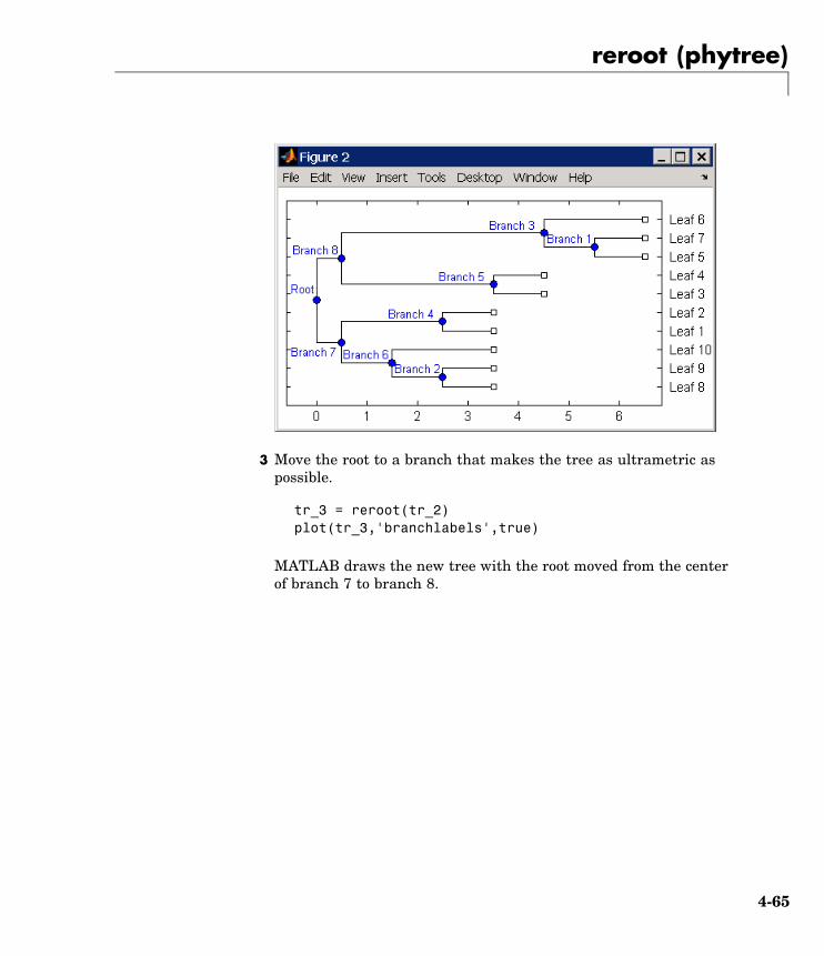
reroot (phytree)
3 Move the root to a branch that makes the tree as ultrametric aspossible.
tr_3 = reroot(tr_2)plot(tr_3,'branchlabels',true)
MATLAB draws the new tree with the root moved from the centerof branch 7 to branch 8.
4-65

reroot (phytree)
See Also Bioinformatics Toolbox
• functions — phytree (object constructor), seqneighjoin
• phytree object methods — get, getbyname, prune, select
4-66
select (phytree)
Purpose Select tree branches and leaves in phytree object
Syntax S = select(Tree, N)[S, Selleaves, Selbranches] = select(...)select(..., 'PropertyName', PropertyValue,...)select(..., 'Reference', ReferenceValue)select(..., 'Criteria', CriteriaValue)select(..., 'Threshold', ThresholdValue)select(..., 'Exclude', ExcludeValue),select(..., 'Propagate', PropagateValue)
ArgumentsTree Phylogenetic tree (phytree object) created with
the function phytree.
N Number of closest nodes to the root node.
ReferenceValue Property to select a reference point formeasuring distance.
CriteriaValue Property to select a criteria for measuringdistance.
ThresholdValue Property to select a distance value. Nodes withdistances below this value are selected.
ExcludeValue Property to remove (exclude) branch orleaf nodes from the output. Enter 'none','branchs', or 'leaves'. The default value is'none'.
PropagateValue Property to select propagating nodes towardthe leaves or the root.
Description S = select(Tree, N) returns a logical vector (S) of size [NumNodesx 1] indicating the N closest nodes to the root node of a phytreeobject (Tree) where NumNodes = NumLeaves + NumBranches. The firstcriterion select uses is branch levels, then patristic distance (also
4-67

select (phytree)
known as tree distance). By default, select uses inf as the value of N,and select(Tree) returns a vector with values of true.
[S, Selleaves, Selbranches] = select(...) returns twoadditional logical vectors, one for the selected leaves and one for theselected branches.
select(..., 'PropertyName', PropertyValue,...) defines optionalproperties using property name/value pairs.
select(..., 'Reference', ReferenceValue) changes the referencepoint(s) to measure the closeness. Reference can be the root (default)or leaves. When using leaves, a node can have multiple distances toits descendant leaves (nonultrametric tree). If this the case, selectconsiders the minimum distance to any descendant leaf.
select(..., 'Criteria', CriteriaValue) changes the criteriaselect uses to measure closeness. If C = 'levels' (default), thefirst criterion is branch levels and then patristic distance. If C ='distance', the first criterion is patristic distance and then branchlevels.
select(..., 'Threshold', ThresholdValue) selects all thenodes where closeness is less than or equal to the threshold value(ThresholdValue). Notice, you can also use either of the properties'criteria' or 'reference', if N is not specified, then N = infF;otherwise you can limit the number of selected nodes by N.
select(..., 'Exclude', ExcludeValue), when ExcludeValue ='branches', sets a postfilter that excludes all the branch nodes from S,or when ExcludeValue = 'leaves', all the leaf nodes. The default is'none'.
select(..., 'Propagate', PropagateValue) activates apostfunctionality that propagates the selected nodes to the leaves whenP=='toleaves' or toward the root finding a common ancestor when P== 'toroot'. The default value is 'none'. P may also be 'both'. The'Propagate' property acts after the 'Exclude' property.
4-68

select (phytree)
Examples % Load a phylogenetic tree created from a protein family:tr = phytreeread('pf00002.tree');
% To find close products for a given protein (e.g. vips_human):ind = getbyname(tr,'vips_human');[sel,sel_leaves] = select(tr,'criteria','distance',...
'threshold',0.6,'reference',ind);view(tr,sel_leaves)
% To find potential outliers in the tree, use[sel,sel_leaves] = select(tr,'criteria','distance',...
'threshold',.3,...'reference','leaves',...'exclude','leaves',...'propagate','toleaves');
view(tr,~sel_leaves)
See Also Bioinformatics Toolbox
• functions — phytree (object constructor), phytreetool
• phytree object methods — get, pdist, prune
4-69
shortestpath (biograph)
Purpose Solve shortest path problem in biograph object
Syntax [dist, path, pred] = shortestpath(BGObj, S)[dist, path, pred] = shortestpath(BGObj, S, T)[...] = shortestpath(..., 'Directed', DirectedValue, ...)[...] = shortestpath(..., 'Method', MethodValue, ...)[...] = shortestpath(..., 'Weights', WeightsValue, ...)
ArgumentsBGObj biograph object created by biograph (object
constructor).
S Node in graph represented by an N-by-N adjacencymatrix extracted from a biograph object, BGObj.
T Node in graph represented by an N-by-N adjacencymatrix extracted from a biograph object, BGObj.
DirectedValue Property that indicates whether the graphrepresented by the N-by-N adjacency matrixextracted from a biograph object, BGObj, is directedor undirected. Enter false for an undirected graph.This results in the upper triangle of the sparsematrix being ignored. Default is true.
4-70

shortestpath (biograph)
MethodValue String that specifies the algorithm used to find theshortest path. Choices are:• 'Bellman-Ford' — Assumes weights of the edges
to be nonzero entries in the N-by-N adjacencymatrix. Time complexity is O(N*E), where N andE are the number of nodes and edges respectively.
• 'BFS' — Breadth-first search. Assumes allweights to be equal, and nonzero entries in theN-by-N adjacency matrix to represent edges.Time complexity is O(N+E), where N and E are thenumber of nodes and edges respectively.
• 'Acyclic' — Assumes the graph represented bythe N-by-N adjacency matrix extracted from abiograph object, BGObj, to be a directed acyclicgraph and that weights of the edges are nonzeroentries in the N-by-N adjacency matrix. Timecomplexity is O(N+E), where N and E are thenumber of nodes and edges respectively.
• 'Dijkstra' — Default algorithm. Assumesweights of the edges to be positive values in theN-by-N adjacency matrix. Time complexity isO(log(N)*E), where N and E are the number ofnodes and edges respectively.
WeightsValue Column vector that specifies custom weights forthe edges in the N-by-N adjacency matrix extractedfrom a biograph object, BGObj. It must have oneentry for every nonzero value (edge) in the N-by-Nadjacency matrix. The order of the custom weightsin the vector must match the order of the nonzerovalues in the N-by-N adjacency matrix when it istraversed column-wise. This property lets you usezero-valued weights. By default, shortestpathsgets weight information from the nonzero entries inthe N-by-N adjacency matrix.
4-71

shortestpath (biograph)
DescriptionTip For introductory information on graph theory functions, see “GraphTheory Functions” in the Bioinformatics Toolbox documentation.
[dist, path, pred] = shortestpath(BGObj, S) determines thesingle-source shortest paths from node S to all other nodes in the graphrepresented by an N-by-N adjacency matrix extracted from a biographobject, BGObj. Weights of the edges are all nonzero entries in the N-by-Nadjacency matrix. dist are the N distances from the source to everynode (using Infs for nonreachable nodes and 0 for the source node).path contains the winning paths to every node. pred contains thepredecessor nodes of the winning paths.
[dist, path, pred] = shortestpath(BGObj, S, T) determines thesingle source-single destination shortest path from node S to node T.
[...] = shortestpath(..., 'PropertyName',PropertyValue, ...) calls shortestpath with optionalproperties that use property name/property value pairs. You canspecify one or more properties in any order. Each PropertyName mustbe enclosed in single quotes and is case insensitive. These propertyname/property value pairs are as follows:
[...] = shortestpath(..., 'Directed', DirectedValue, ...)indicates whether the graph represented by the N-by-N adjacencymatrix extracted from a biograph object, BGObj, is directed orundirected. Set DirectedValue to false for an undirected graph. Thisresults in the upper triangle of the sparse matrix being ignored. Defaultis true.
[...] = shortestpath(..., 'Method', MethodValue, ...) lets youspecify the algorithm used to find the shortest path. Choices are:
• 'Bellman-Ford' — Assumes weights of the edges to be nonzeroentries in the N-by-N adjacency matrix. Time complexity is O(N*E),where N and E are the number of nodes and edges respectively.
4-72

shortestpath (biograph)
• 'BFS' — Breadth-first search. Assumes all weights to be equal, andnonzero entries in the N-by-N adjacency matrix to represent edges.Time complexity is O(N+E), where N and E are the number of nodesand edges respectively.
• 'Acyclic' — Assumes the graph represented by the N-by-Nadjacency matrix extracted from a biograph object, BGObj, to be adirected acyclic graph and that weights of the edges are nonzeroentries in the N-by-N adjacency matrix. Time complexity is O(N+E),where N and E are the number of nodes and edges respectively.
• 'Dijkstra' — Default algorithm. Assumes weights of the edges tobe positive values in the N-by-N adjacency matrix. Time complexityis O(log(N)*E), where N and E are the number of nodes and edgesrespectively.
[...] = shortestpath(..., 'Weights', WeightsValue, ...) lets youspecify custom weights for the edges. WeightsValue is a column vectorhaving one entry for every nonzero value (edge) in the N-by-N adjacencymatrix extracted from a biograph object, BGObj. The order of the customweights in the vector must match the order of the nonzero values inthe N-by-N adjacency matrix when it is traversed column-wise. Thisproperty lets you use zero-valued weights. By default, shortestpathgets weight information from the nonzero entries in the N-by-Nadjacency matrix.
References [1] Dijkstra, E.W. (1959). A note on two problems in connexion withgraphs. Numerische Mathematik 1, 269-271.
[2] Bellman, R. (1958). On a Routing Problem. Quarterly of AppliedMathematics 16(1), 87-90.
[3] Siek, J.G., Lee, L-Q, and Lumsdaine, A. (2002). The Boost GraphLibrary User Guide and Reference Manual, (Upper Saddle River,NJ:Pearson Education).
See Also Bioinformatics Toolbox functions: biograph (object constructor),graphshortestpath
4-73
shortestpath (biograph)
Bioinformatics Toolbox object: biograph object
Bioinformatics Toolbox methods of a biograph object:allshortestpaths, conncomp, isdag, isomorphism, isspantree,maxflow, minspantree, topoorder, traverse
4-74

subtree (phytree)
Purpose Extract phylogenetic subtree
Syntax Tree2 = subtree(Tree1, Nodes)
Description Tree2 = subtree(Tree1, Nodes) extracts a new subtree (Tree2)where the new root is the first common ancestor of the Nodes vectorfrom Tree1. Nodes in the tree are indexed as [1:NUMLEAVES] forthe leaves and as [NUMLEAVES+1:NUMLEAVES+NUMBRANCHES] forthe branches. Nodes can also be a logical array of following sizes[NUMLEAVES+NUMBRANCHES x 1], [NUMLEAVES x 1] or [NUMBRANCHESx 1].
Examples 1 Load a phylogenetic tree created from a protein family.
tr = phytreeread('pf00002.tree')
2 Get the subtree that contains the VIPS and CGRR human proteins.
sel = getbyname(tr,{'vips_human','cgrr_human'});sel = any(sel,2);tr = subtree(tr,sel)view(tr);
See Also Bioinformatics Toolbox
• functions — phytree (object constructor)
• phytree object methods — get, getbyname, prune, select
4-75

topoorder (biograph)
Purpose Perform topological sort of directed acyclic graph extracted frombiograph object
Syntax order = topoorder(BGObj)
ArgumentsBGObj biograph object created by biograph (object constructor).
DescriptionTip For introductory information on graph theory functions, see “GraphTheory Functions” in the Bioinformatics Toolbox documentation.
order = topoorder(BGObj) returns an index vector with the orderof the nodes sorted topologically. In topological order, an edge canexist between a source node u and a destination node v, if and onlyif u appears before v in the vector order. BGObj is a biograph objectfrom which an N-by-N adjacency matrix is extracted and represents adirected acyclic graph (DAG). In the N-by-N sparse matrix, all nonzeroentries indicate the presence of an edge.
References [1] Siek, J.G., Lee, L-Q, and Lumsdaine, A. (2002). The Boost GraphLibrary User Guide and Reference Manual, (Upper Saddle River,NJ:Pearson Education).
See Also Bioinformatics Toolbox functions: biograph (object constructor),graphtopoorder
Bioinformatics Toolbox object: biograph object
Bioinformatics Toolbox methods of a biograph object:allshortestpaths, conncomp, isdag, isomorphism, isspantree,maxflow, minspantree, shortestpath, traverse
4-76

traverse (biograph)
Purpose Traverse biograph object by following adjacent nodes
Syntax [disc, pred, closed] = traverse(BGObj, S)[...] = traverse(BGObj, S, ...'Depth', DepthValue, ...)[...] = traverse(BGObj, S, ...'Directed', DirectedValue, ...)[...] = traverse(BGObj, S, ...'Method', MethodValue, ...)
ArgumentsBGObj biograph object created by biograph (object
constructor).
S Integer that indicates the source node in BGObj.
DepthValue Integer that indicates a node in BGObj that specifiesthe depth of the search. Default is Inf (infinity).
DirectedValue Property that indicates whether graph representedby an N-by-N adjacency matrix extracted from abiograph object, BGObj is directed or undirected.Enter false for an undirected graph. This resultsin the upper triangle of the sparse matrix beingignored. Default is true.
MethodValue String that specifies the algorithm used to traversethe graph. Choices are:• 'BFS' — Breadth-first search. Time complexity
is O(N+E), where N and E are number of nodesand edges respectively.
• 'DFS' — Default algorithm. Depth-first search.Time complexity is O(N+E), where N and E arenumber of nodes and edges respectively.
DescriptionTip For introductory information on graph theory functions, see “GraphTheory Functions” in the Bioinformatics Toolbox documentation.
4-77

traverse (biograph)
[disc, pred, closed] = traverse(BGObj, S) traverses the directedgraph represented by an N-by-N adjacency matrix extracted from abiograph object, BGObj, starting from the node indicated by integer S. Inthe N-by-N sparse matrix, all nonzero entries indicate the presence ofan edge. disc is a vector of node indices in the order in which they arediscovered. pred is a vector of predecessor node indices (listed in theorder of the node indices) of the resulting spanning tree. closed is avector of node indices in the order in which they are closed.
[...] = traverse(BGObj, S, ...'PropertyName',PropertyValue, ...) calls traverse with optional properties thatuse property name/property value pairs. You can specify one or moreproperties in any order. Each PropertyName must be enclosed in singlequotes and is case insensitive. These property name/property valuepairs are as follows:
[...] = traverse(BGObj, S, ...'Depth', DepthValue, ...) specifiesthe depth of the search. DepthValue is an integer indicating a node inthe graph represented by the N-by-N adjacency matrix extracted from abiograph object, BGObj. Default is Inf (infinity).
[...] = traverse(BGObj, S, ...'Directed', DirectedValue, ...)indicates whether the graph represented by the N-by-N adjacencymatrix extracted from a biograph object, BGObj is directed or undirected.Set DirectedValue to false for an undirected graph. This results inthe upper triangle of the sparse matrix being ignored. Default is true.
[...] = traverse(BGObj, S, ...'Method', MethodValue, ...) letsyou specify the algorithm used to traverse the graph represented bythe N-by-N adjacency matrix extracted from a biograph object, BGObj.Choices are:
• 'BFS' — Breadth-first search. Time complexity is O(N+E), where Nand E are number of nodes and edges respectively.
• 'DFS' — Default algorithm. Depth-first search. Time complexity isO(N+E), where N and E are number of nodes and edges respectively.
4-78

traverse (biograph)
References [1] Sedgewick, R., (2002). Algorithms in C++, Part 5 Graph Algorithms(Addison-Wesley).
[2] Siek, J.G., Lee, L-Q, and Lumsdaine, A. (2002). The Boost GraphLibrary User Guide and Reference Manual, (Upper Saddle River,NJ:Pearson Education).
See Also Bioinformatics Toolbox functions: biograph (object constructor),graphtraverse
Bioinformatics Toolbox object: biograph object
Bioinformatics Toolbox methods of a biograph object:allshortestpaths, conncomp, isdag, isomorphism, isspantree,maxflow, minspantree, shortestpath, topoorder
4-79
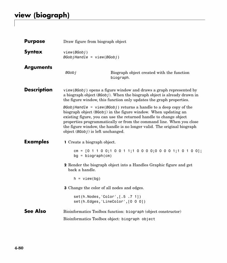
view (biograph)
Purpose Draw figure from biograph object
Syntax view(BGobj)BGobjHandle = view(BGobj)
ArgumentsBGobj Biograph object created with the function
biograph.
Description view(BGobj) opens a figure window and draws a graph represented bya biograph object (BGobj). When the biograph object is already drawn inthe figure window, this function only updates the graph properties.
BGobjHandle = view(BGobj) returns a handle to a deep copy of thebiograph object (BGobj) in the figure window. When updating anexisting figure, you can use the returned handle to change objectproperties programmatically or from the command line. When you closethe figure window, the handle is no longer valid. The original biographobject (BGobj) is left unchanged.
Examples 1 Create a biograph object.
cm = [0 1 1 0 0;1 0 0 1 1;1 0 0 0 0;0 0 0 0 1;1 0 1 0 0];bg = biograph(cm)
2 Render the biograph object into a Handles Graphic figure and getback a handle.
h = view(bg)
3 Change the color of all nodes and edges.
set(h.Nodes,'Color',[.5 .7 1])set(h.Edges,'LineColor',[0 0 0])
See Also Bioinformatics Toolbox function: biograph (object constructor)
Bioinformatics Toolbox object: biograph object
4-80

view (biograph)
Bioinformatics Toolbox methods of a biograph object: dolayout,getancestors, getdescendants, getedgesbynodeid, getnodesbyid,getrelatives, view
MATLAB functions: get, set
4-81

view (phytree)
Purpose View phylogenetic tree
Syntax view(Tree)view(Tree, IntNodes)
ArgumentsTree Phylogenetic tree (phytree object) created with the
function phytree.
IntNodes Nodes from the phytree object to initially display inthe Tree.
Description view(Tree) opens the Phylogenetic Tree Tool window and draws a treefrom data in a phytree object (Tree). The significant distances betweenbranches and nodes are in the horizontal direction. Vertical distanceshave no significance and are selected only for display purposes. You canaccess tools to edit and analyze the tree from the Phylogenetic Tree Toolmenu bar or by using the left and right mouse buttons.
view(Tree, IntNodes) opens the Phylogenetic Tree Tool window withan initial selection of nodes specified by IntNodes. IntNodes can be alogical array of any of the following sizes: NumLeaves + NumBranches x1, NumLeaves x 1, or NumBranches x 1. IntNodes can also be a list ofindices.
Example tree = phytreeread('pf00002.tree')view(tree)
See Also Bioinformatics Toolbox functions: phytree (object constructor),phytreeread, phytreetool, seqlinkage, seqneighjoin
Bioinformatics Toolbox object: phytree object
Bioinformatics Toolbox method of phytree object: plot
4-82

weights (phytree)
Purpose Calculate weights for phylogenetic tree
Syntax W = weights(Tree)
ArgumentsTree Phylogenetic tree (phytree object) created with
the function phytree.
Description W = weights(Tree) calculates branch proportional weights for everyleaf in a tree (Tree) using the Thompson-Higgins-Gibson method. Thedistance of every segment of the tree is adjusted by dividing it by thenumber of leaves it contains. The sequence weights are the result ofnormalizing to unity the new patristic distances between every leafand the root.
Examples 1 Create an ultrametric tree with specified branch distances.
bd = [1 2 3]';tr_1 = phytree([1 2;3 4;5 6],bd)
2 View the tree.
view(tr_1)
4-83
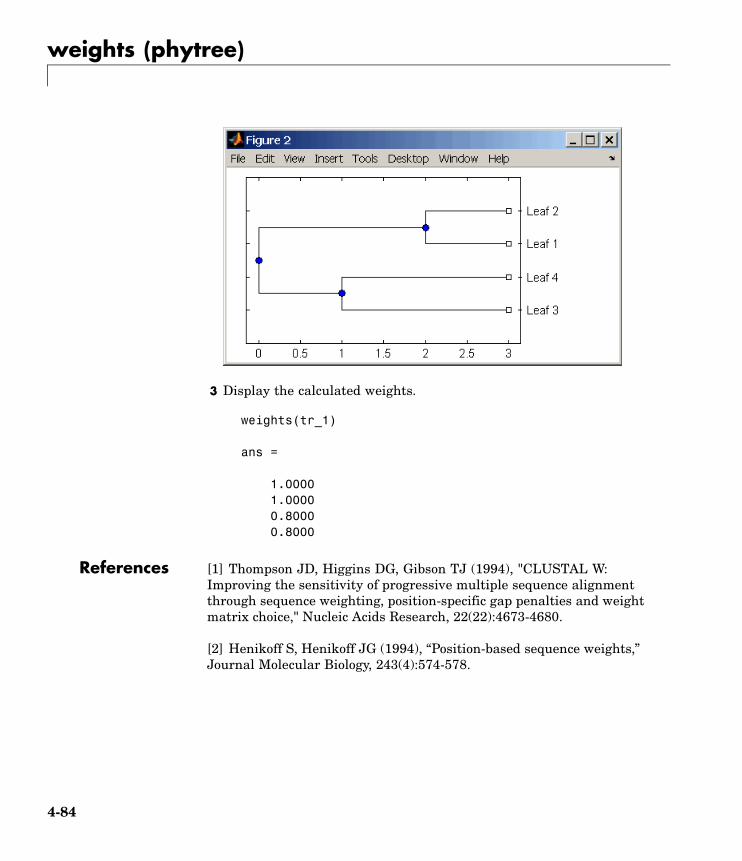
weights (phytree)
3 Display the calculated weights.
weights(tr_1)
ans =
1.00001.00000.80000.8000
References [1] Thompson JD, Higgins DG, Gibson TJ (1994), "CLUSTAL W:Improving the sensitivity of progressive multiple sequence alignmentthrough sequence weighting, position-specific gap penalties and weightmatrix choice," Nucleic Acids Research, 22(22):4673-4680.
[2] Henikoff S, Henikoff JG (1994), “Position-based sequence weights,”Journal Molecular Biology, 243(4):574-578.
4-84
weights (phytree)
See Also Bioinformatics Toolbox
• functions — multialign, phytree (object constructor), profalign,seqlinkage
4-85


5
Objects — Alphabetical List

biograph object
Purpose Data structure containing generic interconnected data used toimplement directed graph
Description A biograph object is a data structure containing generic interconnecteddata used to implement a directed graph. Nodes represent proteins,genes, or any other biological entity, and edges represent interactions,dependences, or any other relationship between the nodes. A biographobject also stores information, such as color properties and text labelcharacteristics, used to create a 2-D visualization of the graph.
You create a biograph object using the object constructor functionbiograph. You can view a graphical representation of a biograph objectusing the view method.
MethodSummary
Following are methods of a biograph object:
allshortestpaths (biograph) Find all shortest paths inbiograph object
conncomp (biograph) Find strongly or weakly connectedcomponents in biograph object
dolayout (biograph) Calculate node positions and edgetrajectories
getancestors (biograph) Find ancestors in biograph object
getdescendants (biograph) Find descendants in biographobject
getedgesbynodeid (biograph) Get handles to edges in biographobject
getmatrix (biograph) Get connection matrix frombiograph object
getnodesbyid (biograph) Get handles to nodes
getrelatives (biograph) Find relatives in biograph object
isdag (biograph) Test for cycles in biograph object
5-2

biograph object
isomorphism (biograph) Find isomorphism between twobiograph objects
isspantree (biograph) Determine if tree created frombiograph object is spanning tree
maxflow (biograph) Calculate maximum flow andminimum cut in biograph object
minspantree (biograph) Find minimal spanning tree inbiograph object
shortestpath (biograph) Solve shortest path problem inbiograph object
topoorder (biograph) Perform topological sort ofdirected acyclic graph extractedfrom biograph object
traverse (biograph) Traverse biograph object byfollowing adjacent nodes
view (biograph) Draw figure from biograph object
Following are methods of a node object:
getancestors (biograph) Find ancestors in biograph object
getdescendants (biograph) Find descendants in biographobject
getrelatives (biograph) Find relatives in biograph object
PropertySummary
A biograph object contains two objects, node objects and edge objects,that have their own properties. For a list of the properties of nodeobjects and edge objects, see the following tables.
5-3
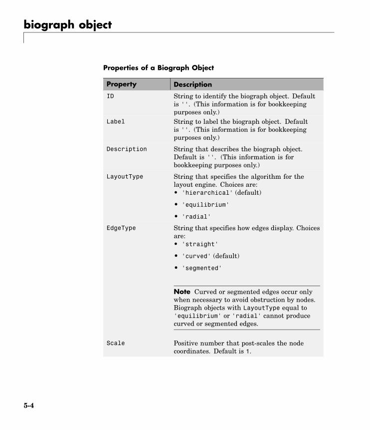
biograph object
Properties of a Biograph Object
Property Description
ID String to identify the biograph object. Defaultis ''. (This information is for bookkeepingpurposes only.)
Label String to label the biograph object. Defaultis ''. (This information is for bookkeepingpurposes only.)
Description String that describes the biograph object.Default is ''. (This information is forbookkeeping purposes only.)
LayoutType String that specifies the algorithm for thelayout engine. Choices are:• 'hierarchical' (default)
• 'equilibrium'
• 'radial'
EdgeType String that specifies how edges display. Choicesare:• 'straight'
• 'curved' (default)
• 'segmented'
Note Curved or segmented edges occur onlywhen necessary to avoid obstruction by nodes.Biograph objects with LayoutType equal to'equilibrium' or 'radial' cannot producecurved or segmented edges.
Scale Positive number that post-scales the nodecoordinates. Default is 1.
5-4
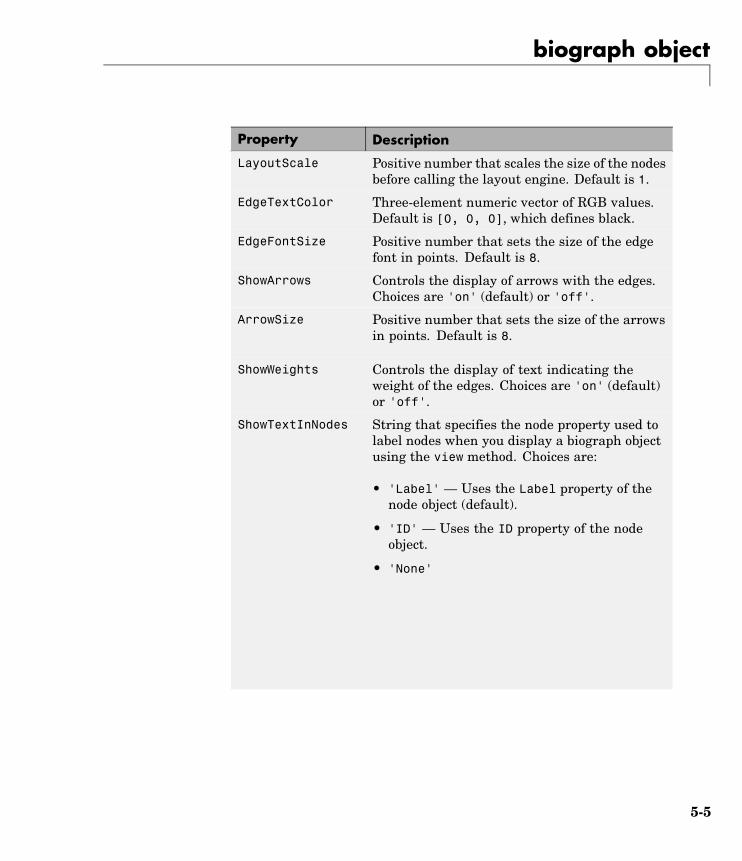
biograph object
Property Description
LayoutScale Positive number that scales the size of the nodesbefore calling the layout engine. Default is 1.
EdgeTextColor Three-element numeric vector of RGB values.Default is [0, 0, 0], which defines black.
EdgeFontSize Positive number that sets the size of the edgefont in points. Default is 8.
ShowArrows Controls the display of arrows with the edges.Choices are 'on' (default) or 'off'.
ArrowSize Positive number that sets the size of the arrowsin points. Default is 8.
ShowWeights Controls the display of text indicating theweight of the edges. Choices are 'on' (default)or 'off'.
ShowTextInNodes String that specifies the node property used tolabel nodes when you display a biograph objectusing the view method. Choices are:
• 'Label' — Uses the Label property of thenode object (default).
• 'ID' — Uses the ID property of the nodeobject.
• 'None'
5-5

biograph object
Property Description
NodeAutoSize Controls precalculating the node size beforecalling the layout engine. Choices are 'on'(default) or 'off'.
NodeCallback User-defined callback for all nodes. Enterthe name of a function, a function handle, ora cell array with multiple function handles.After using the view function to display thebiograph object in the Biograph Viewer, you candouble-click a node to activate the first callback,or right-click and select a callback to activate.Default is the anonymous function, @(node)inspect(node), which displays the PropertyInspector dialog box.
EdgeCallback User-defined callback for all edges. Enterthe name of a function, a function handle, ora cell array with multiple function handles.After using the view function to display thebiograph object in the Biograph Viewer, youcan double-click an edge to activate the firstcallback, or right-click and select a callback toactivate. Default is the anonymous function,@(edge) inspect(edge), which displays theProperty Inspector dialog box.
CustomNodeDrawFcn Function handle to customized function to drawnodes. Default is [].
5-6
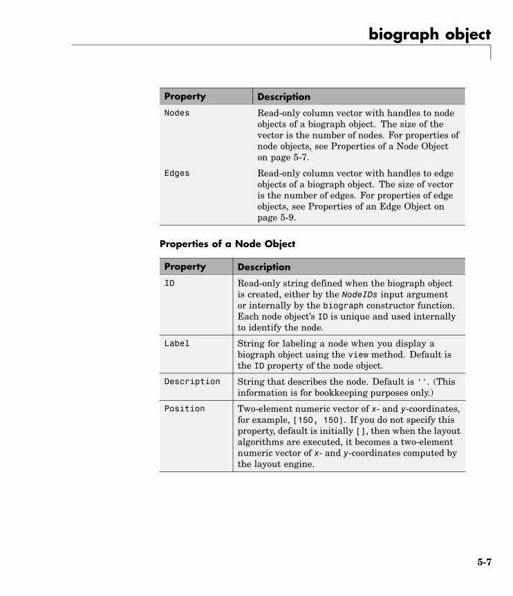
biograph object
Property Description
Nodes Read-only column vector with handles to nodeobjects of a biograph object. The size of thevector is the number of nodes. For properties ofnode objects, see Properties of a Node Objecton page 5-7.
Edges Read-only column vector with handles to edgeobjects of a biograph object. The size of vectoris the number of edges. For properties of edgeobjects, see Properties of an Edge Object onpage 5-9.
Properties of a Node Object
Property Description
ID Read-only string defined when the biograph objectis created, either by the NodeIDs input argumentor internally by the biograph constructor function.Each node object’s ID is unique and used internallyto identify the node.
Label String for labeling a node when you display abiograph object using the view method. Default isthe ID property of the node object.
Description String that describes the node. Default is ''. (Thisinformation is for bookkeeping purposes only.)
Position Two-element numeric vector of x- and y-coordinates,for example, [150, 150]. If you do not specify thisproperty, default is initially [], then when the layoutalgorithms are executed, it becomes a two-elementnumeric vector of x- and y-coordinates computed bythe layout engine.
5-7

biograph object
Property Description
Shape String that specifies the shape of the nodes. Choicesare:• 'box'(default)
• 'ellipse'
• 'circle'
• 'rectangle'
• 'diamond'
• 'trapezium'
• 'invtrapezium'
• 'house'
• 'inverse'
• 'parallelogram'
Size Two-element numeric vector calculated beforecalling the layout engine using the actual font sizeand shape of the node. Default is [10, 10].
Color Three-element numeric vector of RGB values thatspecifies the fill color of the node. Default is [1, 1,0.7], which defines yellow.
LineWidth Positive number. Default is 1.
LineColor Three-element numeric vector of RGB values thatspecifies the outline color of the node. Default is[0.3, 0.3, 1], which defines blue.
FontSize Positive number that sets the size of the node font inpoints. Default is 8.
5-8

biograph object
Property Description
TextColor Three-element numeric vector of RGB values thatspecifies the color of the node labels. Default is [0,0, 0], which defines black.
UserData Miscellaneous, user-defined data that you want toassociate with the node. The node does not use thisproperty, but you can access and specify it using theget and set functions. Default is [].
Properties of an Edge Object
Property Description
ID Read-only string defined when the biograph objectis created, internally by the biograph constructorfunction. Each edge object’s ID is unique and usedinternally to identify the edge.
Label String for labeling an edge when you display abiograph object using the view method. Default isthe ID property of the edge object.
Description String that describes the edge. Default is ''. (Thisinformation is for bookkeeping purposes only.)
Weight Value that represents the weight (cost, distance,length, or capacity) associated with the edge.Default is 1.
LineWidth Positive number. Default is 1.
LineColor Three-element numeric vector of RGB values thatspecifies the color of the edge. Default is [0.5, 0.5,0.5], which defines gray.
UserData Miscellaneous, user-defined data that you want toassociate with the edge. The edge does not use thisproperty, but you can access and specify it using theget and set functions. Default is [].
5-9
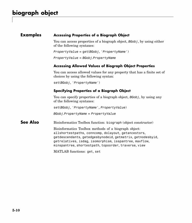
biograph object
Examples Accessing Properties of a Biograph Object
You can access properties of a biograph object, BGobj, by using eitherof the following syntaxes:
PropertyValue = get(BGobj, 'PropertyName')
PropertyValue = BGobj.PropertyName
Accessing Allowed Values of Biograph Object Properties
You can access allowed values for any property that has a finite set ofchoices by using the following syntax:
set(BGobj, 'PropertyName')
Specifying Properties of a Biograph Object
You can specify properties of a biograph object, BGobj, by using anyof the following syntaxes:
set(BGobj, 'PropertyName', PropertyValue)
BGobj.PropertyName = PropertyValue
See Also Bioinformatics Toolbox function: biograph (object constructor)
Bioinformatics Toolbox methods of a biograph object:allshortestpaths, conncomp, dolayout, getancestors,getdescendants, getedgesbynodeid, getmatrix, getnodesbyid,getrelatives, isdag, isomorphism, isspantree, maxflow,minspantree, shortestpath, topoorder, traverse, view
MATLAB functions: get, set
5-10

geneont object
Purpose Data structure containing Gene Ontology (GO) information
Description A geneont object is a data structure containing Gene Ontologyinformation. Gene Ontology terms can be explored and traversedthrough “is_a” and “part_of” relationships.
MethodSummary
Following are methods of a geneont object:
getancestors (geneont) Numeric IDs for ancestors ofGene Ontology term
getdescendants (geneont) Numeric IDs for descendants ofGene Ontology term
getmatrix (geneont) Convert geneont object intorelationship matrix
getrelatives (geneont) Numeric IDs for relatives of GeneOntology term
PropertySummary
Properties of a geneont Object
Property Description
default_namespace Read-only string containing the namespace towhich terms are assigned.
format_version Read-only string containing the version of theencoding of the OBO flat format file.
date Read-only string containing the date the OBOfile was last updated.
Terms Read-only column vector with handles to termobjects of a geneont object. For properties ofterm objects, see Properties of Terms Objectson page 5-12.
5-11

geneont object
Properties of Terms Objects
Property Description
id Numeric value that corresponds to the GO ID ofthe GO term.
Tip You can use the num2goid function to convertid to a GO ID string.
name String representing the name of the GO term.
ontology String limited to 'molecular function','biological process', or 'cellularcomponent'.
definition String that defines the GO term.
synonym Numeric array containing GO IDs of GO termsthat are synonyms of this GO term.
is_a Numeric array containing GO IDs of GO termsthat have an “is_a” relationship with this GOterm.
part_of Numeric array containing GO IDs that of GOterms that have a “part_of” relationship with thisGO term.
obsolete Boolean value that indicates if the GO term isobsolete (1) or not obsolete (0).
See Also Bioinformatics Toolbox functions: geneont (object constructor),goannotread, num2goid
Bioinformatics Toolbox methods of geneont object: getancestors,getdescendants, getmatrix, getrelatives
5-12

phytree object
Purpose Data structure containing phylogenetic tree
Description A phytree object is a data structure containing a phylogenetic tree.Phylogenetic trees are binary rooted trees, which means that eachbranch is the parent of two other branches, two leaves, or one branchand one leaf. A phytree object can be ultrametric or nonultrametric.
MethodSummary
Following are methods of a phytree object:
get (phytree) Information about phylogenetictree object
getbyname (phytree) Branches and leaves from phytreeobject
getcanonical (phytree) Calculate canonical form ofphylogenetic tree
getmatrix (phytree) Convert phytree object intorelationship matrix
getnewickstr (phytree) Create Newick-formatted string
pdist (phytree) Calculate pair-wise patristicdistances in phytree object
plot (phytree) Draw phylogenetic tree
prune (phytree) Remove branch nodes fromphylogenetic tree
reorder (phytree) Reorder leaves of phylogenetictree
reroot (phytree) Change root of phylogenetic tree
select (phytree) Select tree branches and leavesin phytree object
subtree (phytree) Extract phylogenetic subtree
5-13

phytree object
view (phytree) View phylogenetic tree
weights (phytree) Calculate weights forphylogenetic tree
PropertySummary Note You cannot modify these properties directly. You can access these
properties using the get method.
Property Description
NumLeaves Number of leaves
NumBranches Number of branches
NumNodes Number of nodes (NumLeaves + NumBranches)
Pointers Branch to leaf/branch connectivity list
Distances Edge length for every leaf/branch
LeafNames Names of the leaves
BranchNames Names of the branches
NodeNames Names of all the nodes
See Also Bioinformatics Toolbox functions: phytree (object constructor),phytreeread, phytreetool, phytreewrite, seqlinkage,seqneighjoin, seqpdist
Bioinformatics Toolbox methods of phytree object: get, getbyname,getcanonical, getmatrix, getnewickstr, pdist, plot, prune, reroot,select, subtree, view, weights
5-14
Index
IndexAaa2int function
reference 2-2aa2nt function
reference 2-5aacount function
reference 2-10affyinvarsetnorm function
reference 2-14affyprobeaffinities function
reference 2-22affyprobeseqread function
reference 2-29affyread function
reference 2-34agferead function
reference 2-39allshortestpaths method
reference 4-2aminolookup function
reference 2-41atomiccomp function
reference 2-46
Bbasecount function
reference 2-48baselookup function
reference 2-52biograph constructor
reference 2-55biograph object
reference 5-2blastncbi function
reference 2-65blastread function
reference 2-73blosum function
reference 2-75
Ccelintensityread function
reference 2-77classperf function
reference 2-82cleave function
reference 2-86clustergram function
reference 2-89codonbias function
reference 2-100codoncount function
reference 2-103conncomp method
reference 4-5cpgisland function
reference 2-107crossvalind function
reference 2-110
Ddayhoff function
reference 2-113dimercount function
reference 2-114dna2rna function
reference 2-117dnds function
reference 2-118dndsml function
reference 2-125dolayout method
reference 4-8
Eemblread function
reference 2-130evalrasmolscript function
Index-1

Index
reference 2-133exprprofrange function
reference 2-135exprprofvar function
reference 2-136
Ffastaread function
reference 2-137fastawrite function
reference 2-140featuresmap
reference 2-142featuresparse
reference 2-152functions
aa2int 2-2aa2nt 2-5aacount 2-10affyinvarsetnorm 2-14affyprobeaffinities 2-22affyprobeseqread 2-29affyread 2-34agferead 2-39aminolookup 2-41atomiccomp 2-46basecount 2-48baselookup 2-52biograph constructor 2-55blastncbi 2-65blastread 2-73blosum 2-75celintensityread 2-77classperf 2-82cleave 2-86clustergram 2-89codonbias 2-100codoncount 2-103cpgisland 2-107
crossvalind 2-110dayhoff 2-113dimercount 2-114dna2rna 2-117dnds 2-118dndsml 2-125emblread 2-130evalrasmolscript 2-133exprprofrange 2-135exprprofvar 2-136fastaread 2-137fastawrite 2-140featuresmap 2-142featuresparse 2-152galread 2-158gcrma 2-159gcrmabackadj 2-168genbankread 2-177geneentropyfilter 2-179genelowvalfilter 2-181geneont 2-183generangefilter 2-186geneticcode 2-188genevarfilter 2-190genpeptread 2-192geosoftread 2-195getblast 2-197getembl 2-200getgenbank 2-203getgenpept 2-206getgeodata 2-209gethmmalignment 2-211gethmmprof 2-215gethmmtree 2-220getpdb 2-222goannotread 2-229gonnet 2-231gprread 2-232graphallshortestpaths 2-235graphconncomp 2-242
Index-2
Index
graphisdag 2-249graphisomorphism 2-255graphisspantree 2-262graphmaxflow 2-264graphminspantree 2-272graphpred2path 2-278graphshortestpath 2-282graphtopoorder 2-294graphtraverse 2-298hmmprofalign 2-307hmmprofestimate 2-310hmmprofgenerate 2-313hmmprofmerge 2-315hmmprofstruct 2-317imageneread 2-323int2aa 2-326int2nt 2-329isoelectric 2-332jcampread 2-335joinseq 2-338knnclassify 2-339knnimpute 2-346maboxplot 2-350mafdr 2-353magetfield 2-360maimage 2-361mainvarsetnorm 2-363mairplot 2-371maloglog 2-379malowess 2-381manorm 2-383mapcaplot 2-386mattest 2-389mavolcanoplot 2-395molviewer 2-403molweight 2-402msalign 2-411msbackadj 2-425msdotplot 2-430msheatmap 2-436
mslowess 2-446msnorm 2-451mspalign 2-455mspeaks 2-465msppresample 2-478msresample 2-486mssgolay 2-490msviewer 2-492multialign 2-495multialignread 2-504multialignviewer 2-506mzxml2peaks 2-507mzxmlread 2-510nmercount 2-512nt2aa 2-513nt2int 2-518ntdensity 2-520nuc44 2-522num2goid 2-523nwalign 2-524oligoprop 2-531optimalleaforder 2-540palindromes 2-544pam 2-546pdbdistplot 2-548pdbread 2-550pdbwrite 2-557pfamhmmread 2-560phytree constructor 2-561phytreeread 2-565phytreetool 2-566phytreewrite 2-568probelibraryinfo 2-570probesetlink 2-572probesetlookup 2-574probesetplot 2-575probesetvalues 2-576profalign 2-578proteinplot 2-581proteinpropplot 2-584
Index-3
Index
quantilenorm 2-590ramachandran 2-591randfeatures 2-593randseq 2-596rankfeatures 2-599rebasecuts 2-604redgreencmap 2-606restrict 2-608revgeneticcode 2-611rmabackadj 2-615rmasummary 2-620rna2dna 2-624scfread 2-625seq2regexp 2-628seqcomplement 2-631seqconsensus 2-632seqdisp 2-634seqdotplot 2-636seqinsertgaps 2-638seqlinkage 2-641seqlogo 2-643seqmatch 2-650seqneighjoin 2-651seqpdist 2-654seqprofile 2-665seqrcomplement 2-668seqreverse 2-669seqshoworfs 2-670seqshowwords 2-675seqtool 2-678seqwordcount 2-680showalignment 2-682showhmmprof 2-685sptread 2-687svmclassify 2-689svmsmoset 2-696svmtrain 2-700swalign 2-716traceplot 2-723
Ggalread function
reference 2-158gcrma function
reference 2-159gcrmabackadj function
reference 2-168genbankread function
reference 2-177geneentropyfilter function
reference 2-179genelowvalfilter function
reference 2-181geneont function
reference 2-183geneont object
reference 5-11generangefilter function
reference 2-186geneticcode function
reference 2-188genevarfilter function
reference 2-190genpeptread function
reference 2-192geosoftread function
reference 2-195get method
reference 4-11getancestors method
biograph object 4-13geneont object 4-16
getblast functionreference 2-197
getbyname methodreference 4-20
getcanonical methodreference 4-22
getdescendants methodbiograph object 4-24
Index-4

Index
geneont object 4-27getedgesbynodeid method
reference 4-29getembl function
reference 2-200getgenbank function
reference 2-203getgenpept function
reference 2-206getgeodata function
reference 2-209gethmmalignment function
reference 2-211gethmmprof function
reference 2-215gethmmtree function
reference 2-220getmatrix (biograph) method
reference 4-31getmatrix (geneont) method
reference 4-32getmatrix (phytree) method
reference 4-33getnewickstr method
reference 4-34getnodesbyid method
reference 4-36getpdb function
reference 2-222getrelatives method
biograph object 4-38geneont object 4-39
goannotread functionreference 2-229
gonnet functionreference 2-231
gprread functionreference 2-232
graphallshortestpaths functionreference 2-235
graphconncomp functionreference 2-242
graphisdag functionreference 2-249
graphisomorphism functionreference 2-255
graphisspantree functionreference 2-262
graphmaxflow functionreference 2-264
graphminspantree functionreference 2-272
graphpred2path functionreference 2-278
graphshortestpath functionreference 2-282
graphtopoorder functionreference 2-294
graphtraverse functionreference 2-298
Hhmmprofalign function
reference 2-307hmmprofestimate function
reference 2-310hmmprofgenerate function
reference 2-313hmmprofmerge function
reference 2-315hmmprofstruct function
reference 2-317
Iimageneread function
reference 2-323int2aa function
reference 2-326
Index-5
Index
int2nt functionreference 2-329
isdag methodreference 4-41
isoelectric functionreference 2-332
isomorphism methodreference 4-42
isspantree methodreference 4-44
Jjcampread function
reference 2-335joinseq function
reference 2-338
Kknnclassify function
reference 2-339knnimpute function
reference 2-346
Mmaboxplot function
reference 2-350mafdr function
reference 2-353magetfield function
reference 2-360maimage function
reference 2-361mainvarsetnorm function
reference 2-363mairplot function
reference 2-371maloglog function
reference 2-379
malowess functionreference 2-381
manorm functionreference 2-383
mapcaplot functionreference 2-386
mattest functionreference 2-389
mavolcanoplot functionreference 2-395
maxflow methodreference 4-45
methodsallshortestpaths 4-2conncomp 4-5dolayout 4-8get 4-11getancestors (biograph) 4-13getancestors (geneont) 4-16getbyname 4-20getcanonical 4-22getdescendants (biograph) 4-24getdescendants (geneont) 4-27getedgesbynodeid 4-29getmatrix (biograph) 4-31getmatrix (geneont) 4-32getmatrix (phytree) 4-33getnewickstr 4-34getnodesbyid 4-36getrelatives (biograph) 4-38getrelatives (geneont) 4-39isdag 4-41isomorphism 4-42isspantree 4-44maxflow 4-45minspantree 4-49pdist 4-52plot 4-54prune 4-57reorder 4-59
Index-6

Index
reroot 4-63select 4-67shortestpath 4-70subtree 4-75topoorder 4-76traverse 4-77view (biograph) 4-80view (phytree) 4-82weights 4-83
minspantree methodreference 4-49
molviewer functionreference 2-403
molweight functionreference 2-402
msalign functionreference 2-411
msbackadj functionreference 2-425
msdotplot functionreference 2-430
msheatmap functionreference 2-436
mslowess functionreference 2-446
msnorm functionreference 2-451
mspalign functionreference 2-455
mspeaks functionreference 2-465
msppresample functionreference 2-478
msresample functionreference 2-486
mssgolay functionreference 2-490
msviewer functionreference 2-492
multialign function
reference 2-495multialignread function
reference 2-504multialignviewer function
reference 2-506mzxml2peaks function
reference 2-507mzxmlread function
reference 2-510
Nnmercount function
reference 2-512nt2aa function
reference 2-513nt2int function
reference 2-518ntdensity function
reference 2-520nuc44 function
reference 2-522num2goid function
reference 2-523nwalign function
reference 2-524
Oobjects
biograph 5-2geneont 5-11phytree 5-13
oligoprop functionreference 2-531
optimalleaforder functionreference 2-540
Ppalindromes function
Index-7

Index
reference 2-544pam function
reference 2-546pdbdistplot function
reference 2-548pdbread function
reference 2-550pdbwrite function
reference 2-557pdist method
reference 4-52pfamhmmread function
reference 2-560phytree constructor
reference 2-561phytree object
reference 5-13phytreeread function
reference 2-565phytreetool function
reference 2-566phytreewrite function
reference 2-568plot method
reference 4-54probelibraryinfo function
reference 2-570probesetlink function
reference 2-572probesetlookup function
reference 2-574probesetplot function
reference 2-575probesetvalues function
reference 2-576profalign function
reference 2-578proteinplot function
reference 2-581proteinpropplot function
reference 2-584prune method
reference 4-57
Qquantilenorm function
reference 2-590
Rramachandran function
reference 2-591randfeatures function
reference 2-593randseq function
reference 2-596rankfeatures function
reference 2-599rebasecuts function
reference 2-604redgreencmap function
reference 2-606reorder method
reference 4-59reroot method
reference 4-63restrict function
reference 2-608revgeneticcode function
reference 2-611rmabackadj function
reference 2-615rmasummary function
reference 2-620rna2dna function
reference 2-624
Sscfread function
Index-8

Index
reference 2-625select method
reference 4-67seq2regexp function
reference 2-628seqcomplement function
reference 2-631seqconsensus function
reference 2-632seqdisp function
reference 2-634seqdotplot function
reference 2-636seqinsertgaps function
reference 2-638seqlinkage function
reference 2-641seqlogo function
reference 2-643seqmatch function
reference 2-650seqneighjoin function
reference 2-651seqpdist function
reference 2-654seqprofile function
reference 2-665seqrcomplement function
reference 2-668seqreverse function
reference 2-669seqshoworfs function
reference 2-670seqshowwords function
reference 2-675seqtool function
reference 2-678seqwordcount function
reference 2-680
shortestpath methodreference 4-70
showalignment functionreference 2-682
showhmmprof functionreference 2-685
sptread functionreference 2-687
subtree methodreference 4-75
svmclassify functionreference 2-689
svmsmoset functionreference 2-696
svmtrain functionreference 2-700
swalign functionreference 2-716
Ttopoorder method
reference 4-76traceplot function
reference 2-723traverse method
reference 4-77
Vview (biograph) method
reference 4-80view (phytree) method
reference 4-82
Wweights method
reference 4-83
Index-9