biological invasions: from critters to mathematicsrobbins/research/usac.pdf · biological...
TRANSCRIPT
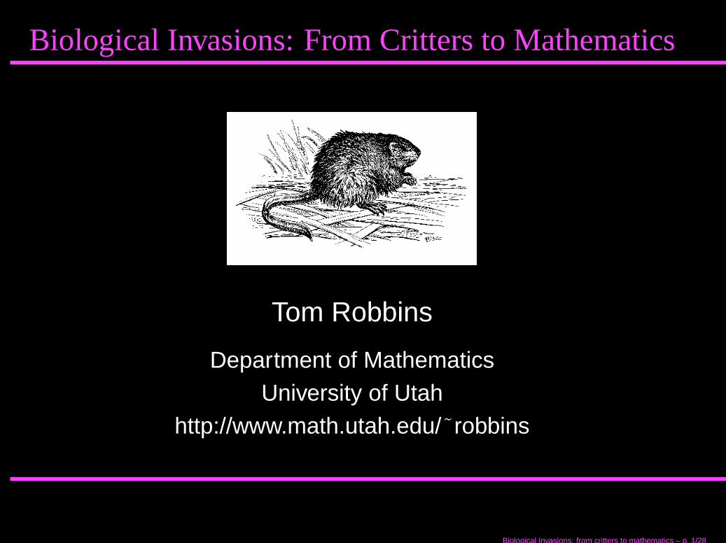
Biological Invasions: From Critters to Mathematics
Tom Robbins
Department of MathematicsUniversity of Utah
http://www.math.utah.edu/˜robbins
Biological Invasions: from critters to mathematics – p. 1/28
Outline
❁ Biology background
❁ Historical example
❁ Model for terrestrial plant species
Biological Invasions: from critters to mathematics – p. 2/28
Outline
❁ Biology background
❁ Historical example
❁ Model for terrestrial plant species
Biological Invasions: from critters to mathematics – p. 2/28
Outline
❁ Biology background
❁ Historical example
❁ Model for terrestrial plant species
Biological Invasions: from critters to mathematics – p. 2/28
Biological Invasions?
❁ What are biological invasions?
❀ A biological invasion is the introduction and spreadof an exotic species within an ecosystem.
❁ Why are biological invasions important?
❀ Economic impact ($100 billion by 1991)
❀ Contribute to the loss of biodiversity
❀ Are a threat to endangered species
Biological Invasions: from critters to mathematics – p. 3/28
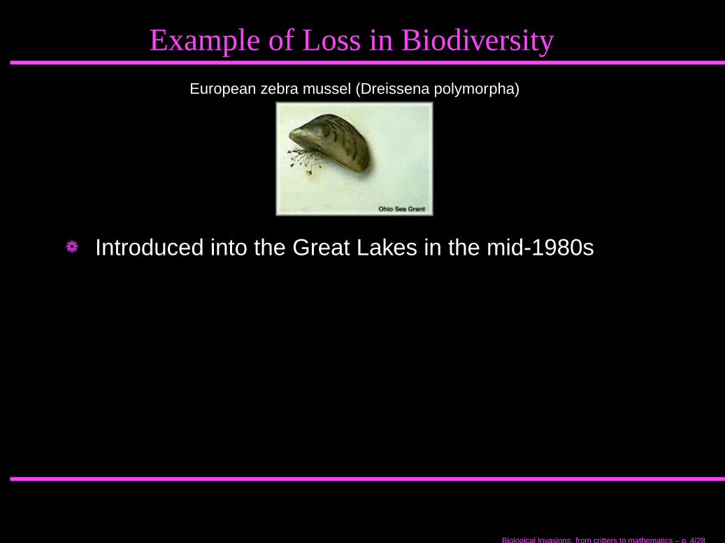
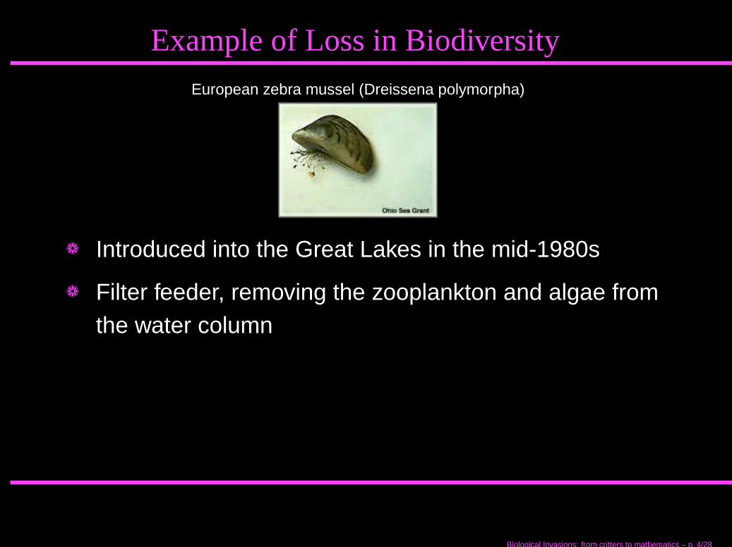
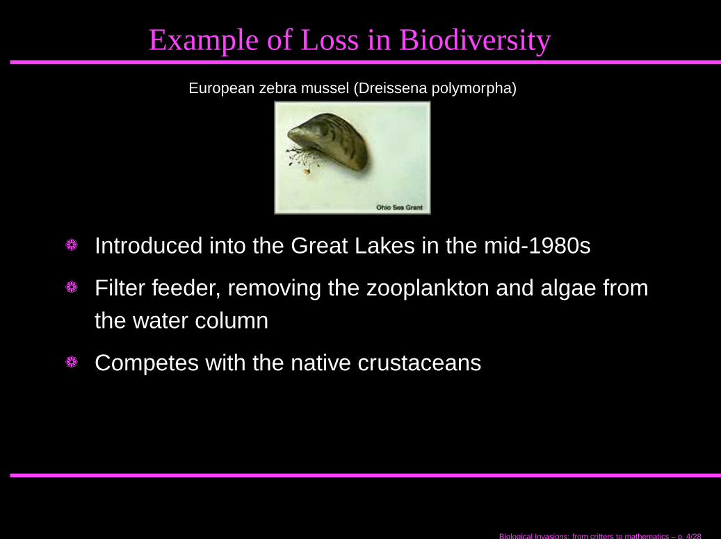
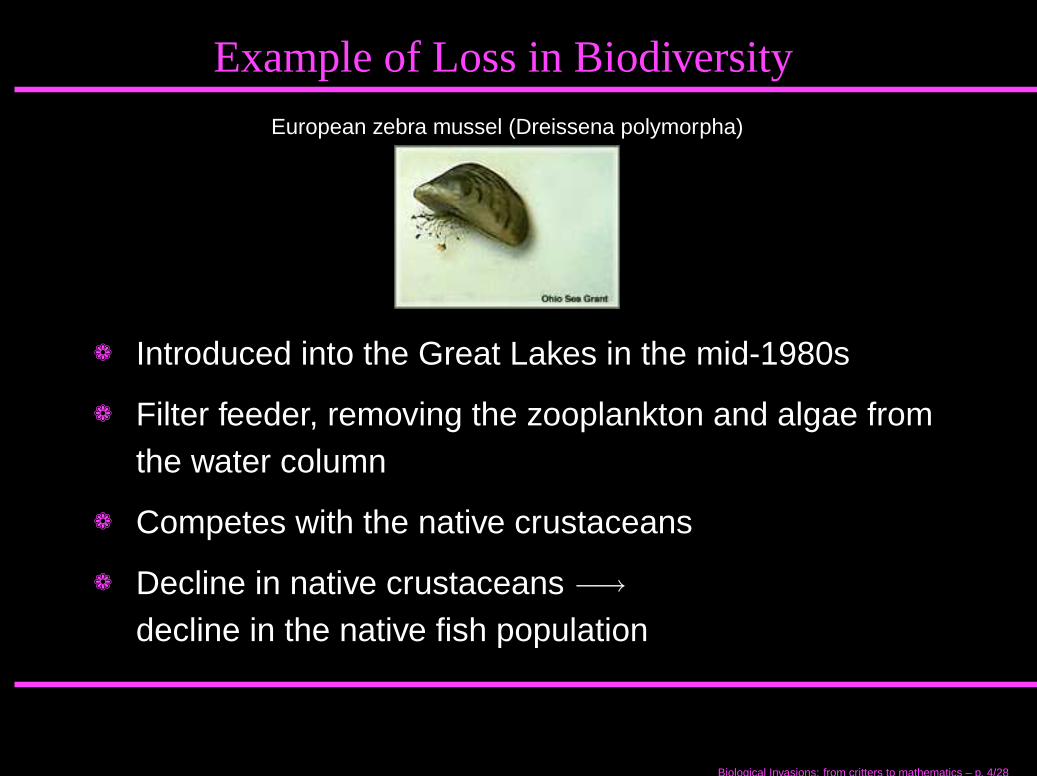
Example of Loss in BiodiversityEuropean zebra mussel (Dreissena polymorpha)
❁ Introduced into the Great Lakes in the mid-1980s
❁ Filter feeder, removing the zooplankton and algae fromthe water column
❁ Competes with the native crustaceans
❁ Decline in native crustaceans −→
decline in the native fish population
Biological Invasions: from critters to mathematics – p. 4/28
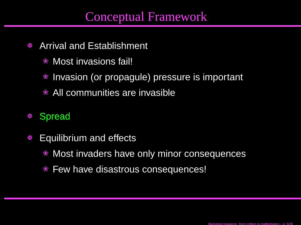
Conceptual Framework
❁ Arrival and Establishment
❀ Most invasions fail!
❀ Invasion (or propagule) pressure is important
❀ All communities are invasible
❁ SpreadSpread
❁ Equilibrium and effects
❀ Most invaders have only minor consequences
❀ Few have disastrous consequences!
Biological Invasions: from critters to mathematics – p. 5/28
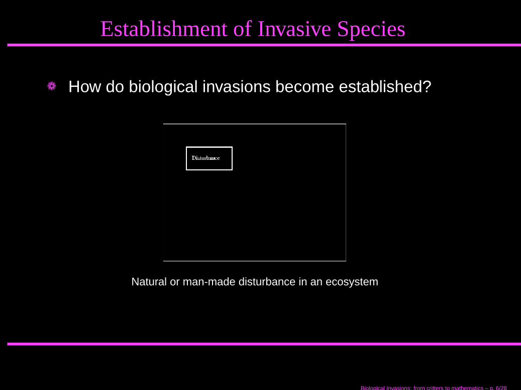
Establishment of Invasive Species
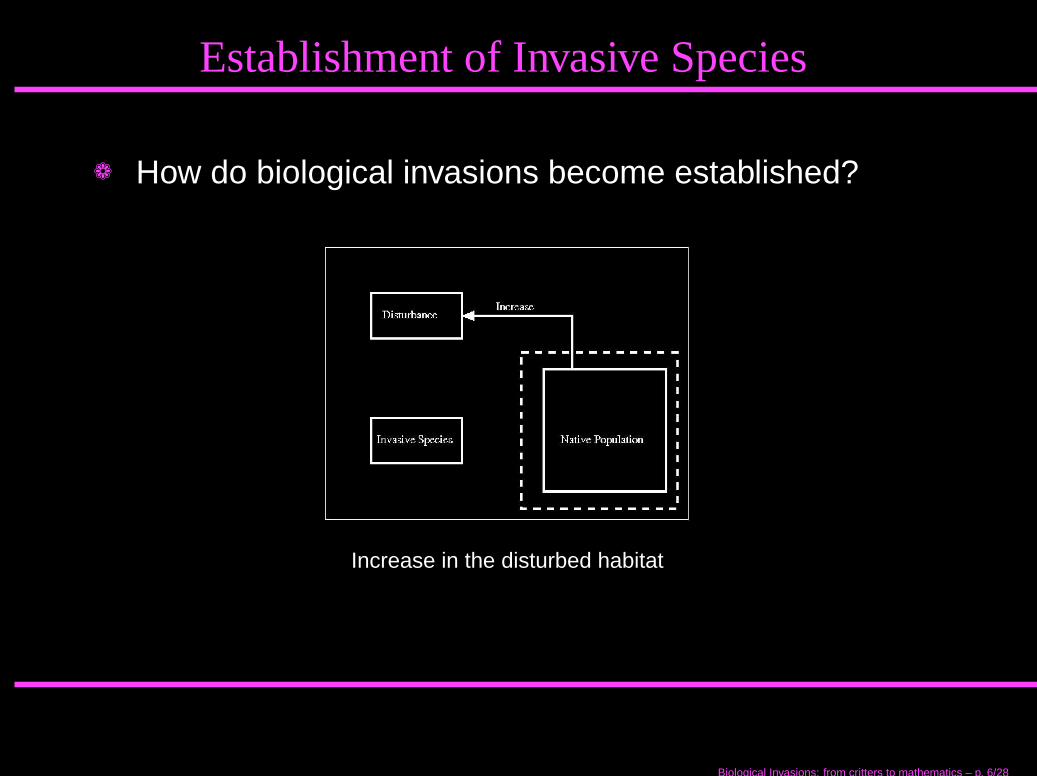
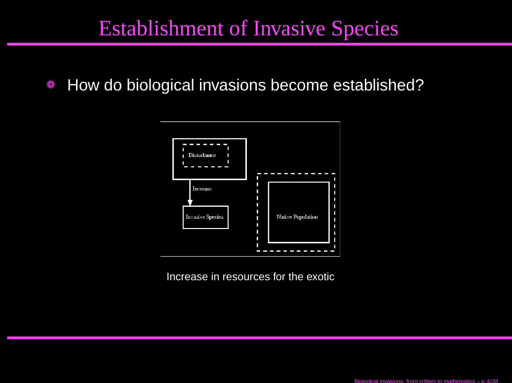
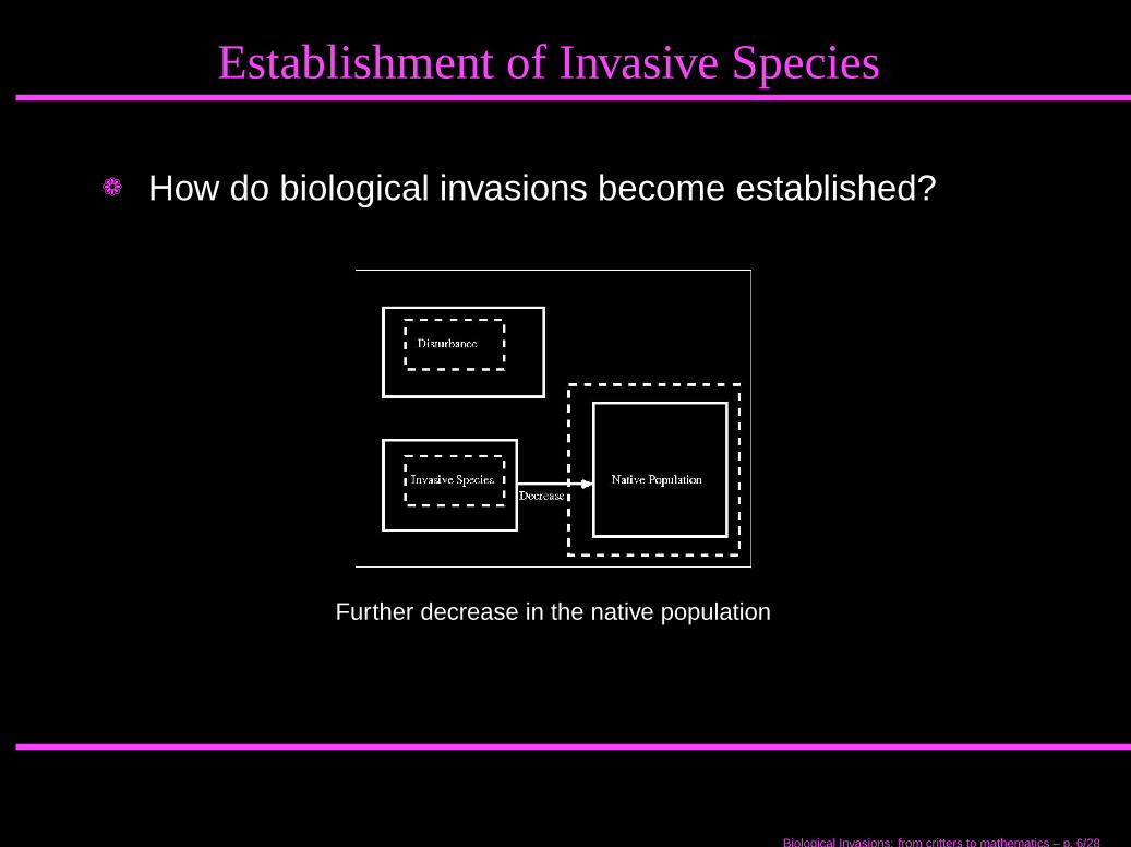
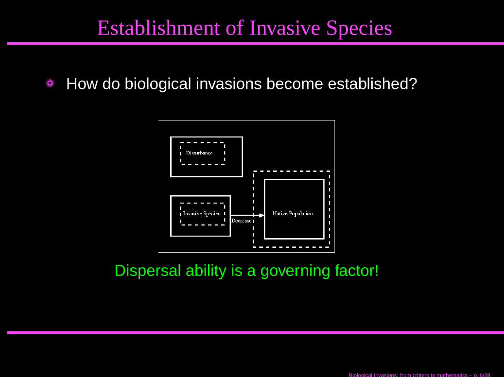
❁ How do biological invasions become established?
Natural or man-made disturbance in an ecosystem
Biological Invasions: from critters to mathematics – p. 6/28
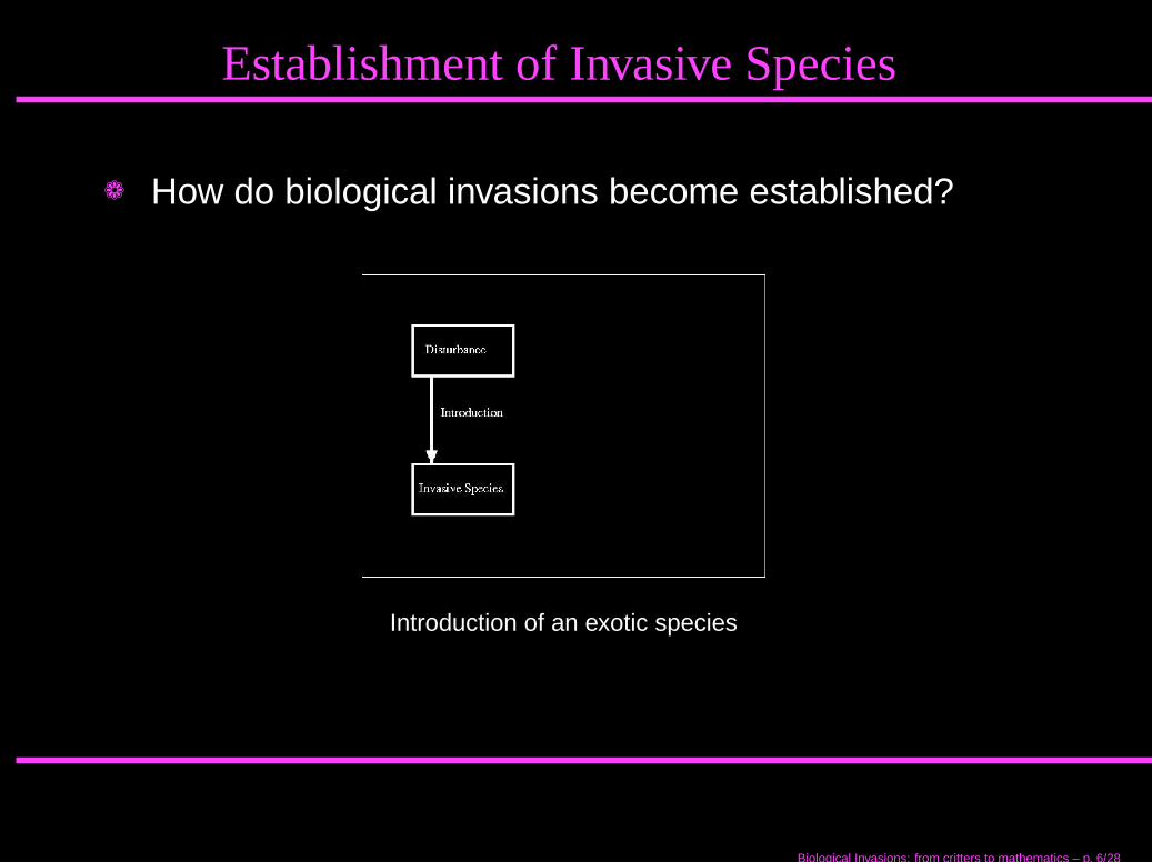
Establishment of Invasive Species
❁ How do biological invasions become established?
Introduction of an exotic species
Biological Invasions: from critters to mathematics – p. 6/28
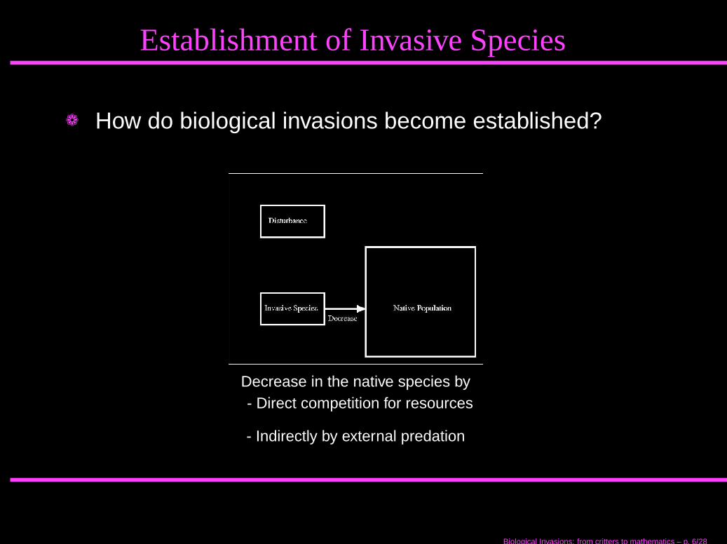
Establishment of Invasive Species
❁ How do biological invasions become established?
Decrease in the native species by- Direct competition for resources
- Indirectly by external predation
Biological Invasions: from critters to mathematics – p. 6/28
Establishment of Invasive Species
❁ How do biological invasions become established?
Increase in the disturbed habitat
Biological Invasions: from critters to mathematics – p. 6/28
Establishment of Invasive Species
❁ How do biological invasions become established?
Increase in resources for the exotic
Biological Invasions: from critters to mathematics – p. 6/28
Establishment of Invasive Species
❁ How do biological invasions become established?
Further decrease in the native population
Biological Invasions: from critters to mathematics – p. 6/28
Establishment of Invasive Species
❁ How do biological invasions become established?
Dispersal ability is a governing factor!
Biological Invasions: from critters to mathematics – p. 6/28
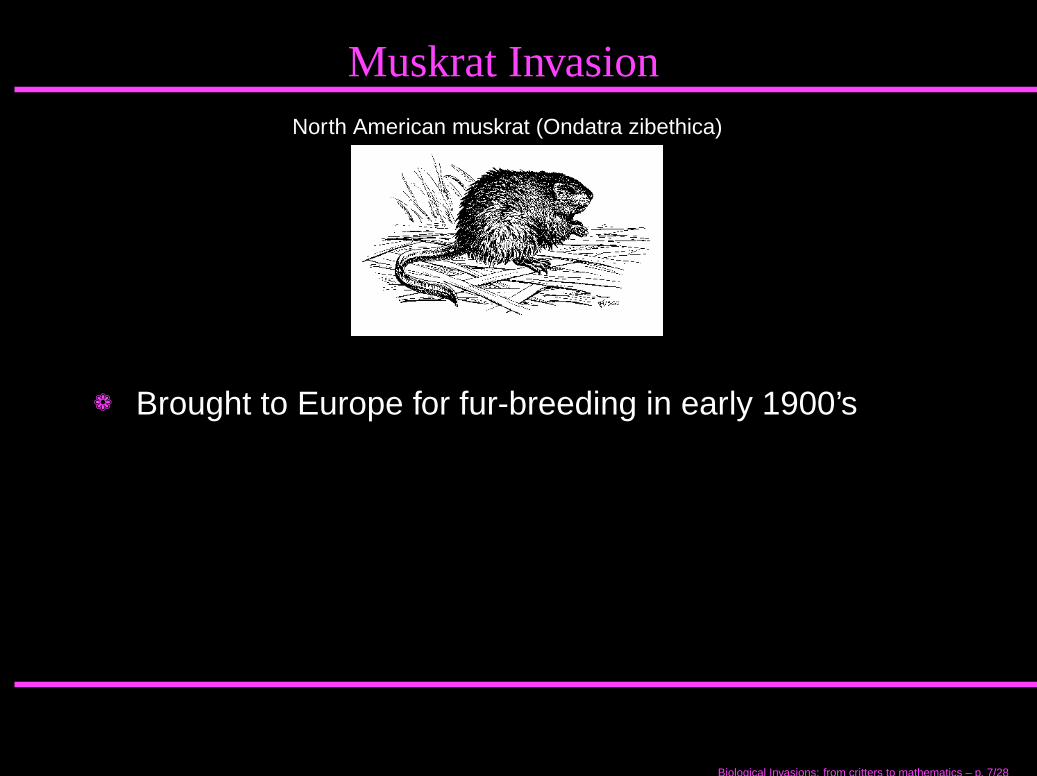
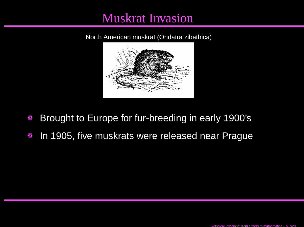
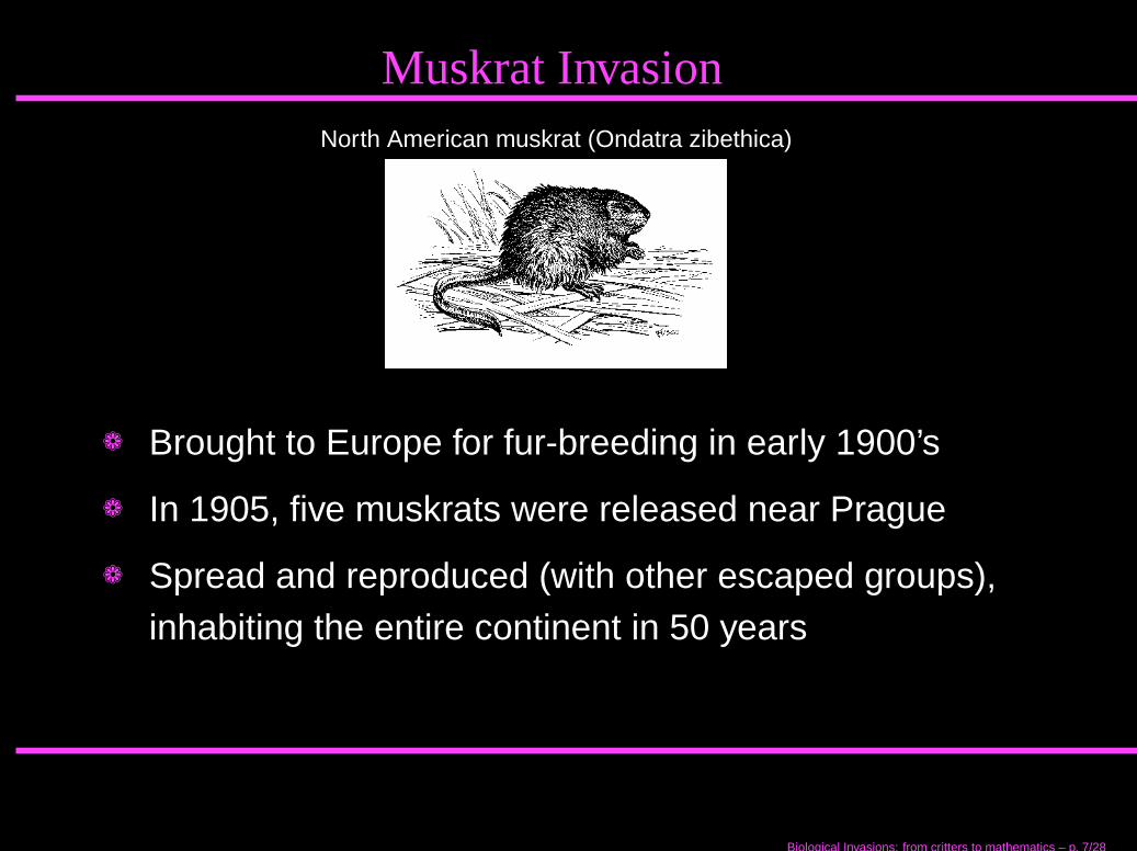
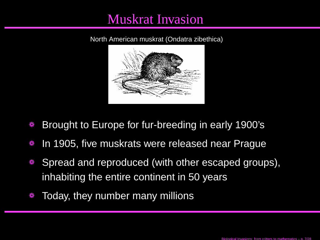
Muskrat InvasionNorth American muskrat (Ondatra zibethica)
❁ Brought to Europe for fur-breeding in early 1900’s
❁ In 1905, five muskrats were released near Prague
❁ Spread and reproduced (with other escaped groups),inhabiting the entire continent in 50 years
❁ Today, they number many millions
Biological Invasions: from critters to mathematics – p. 7/28

Spread of North American Muskrat
� �� �
� �
t = 1905 (initial introduction)
Biological Invasions: from critters to mathematics – p. 8/28
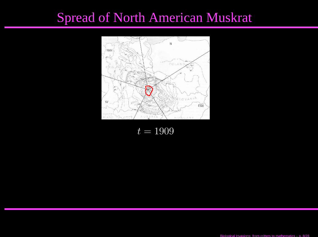
Spread of North American Muskrat
t = 1909
Biological Invasions: from critters to mathematics – p. 8/28
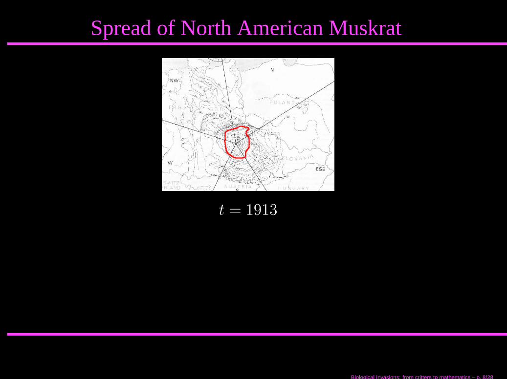
Spread of North American Muskrat
t = 1913
Biological Invasions: from critters to mathematics – p. 8/28

Spread of North American Muskrat
t = 1917
Biological Invasions: from critters to mathematics – p. 8/28
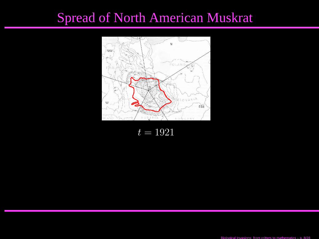
Spread of North American Muskrat
t = 1921
Biological Invasions: from critters to mathematics – p. 8/28
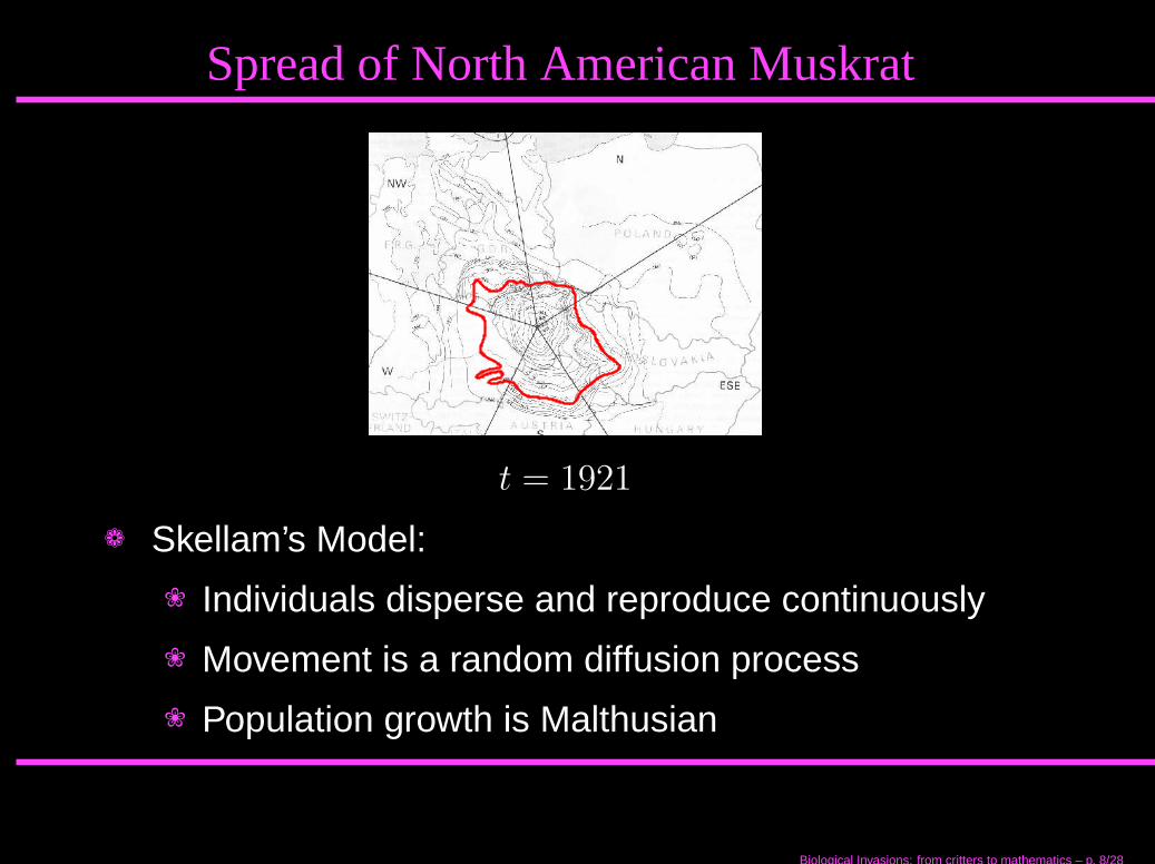
Spread of North American Muskrat
t = 1921
❁ Skellam’s Model:
❀ Individuals disperse and reproduce continuously
❀ Movement is a random diffusion process
❀ Population growth is Malthusian
Biological Invasions: from critters to mathematics – p. 8/28
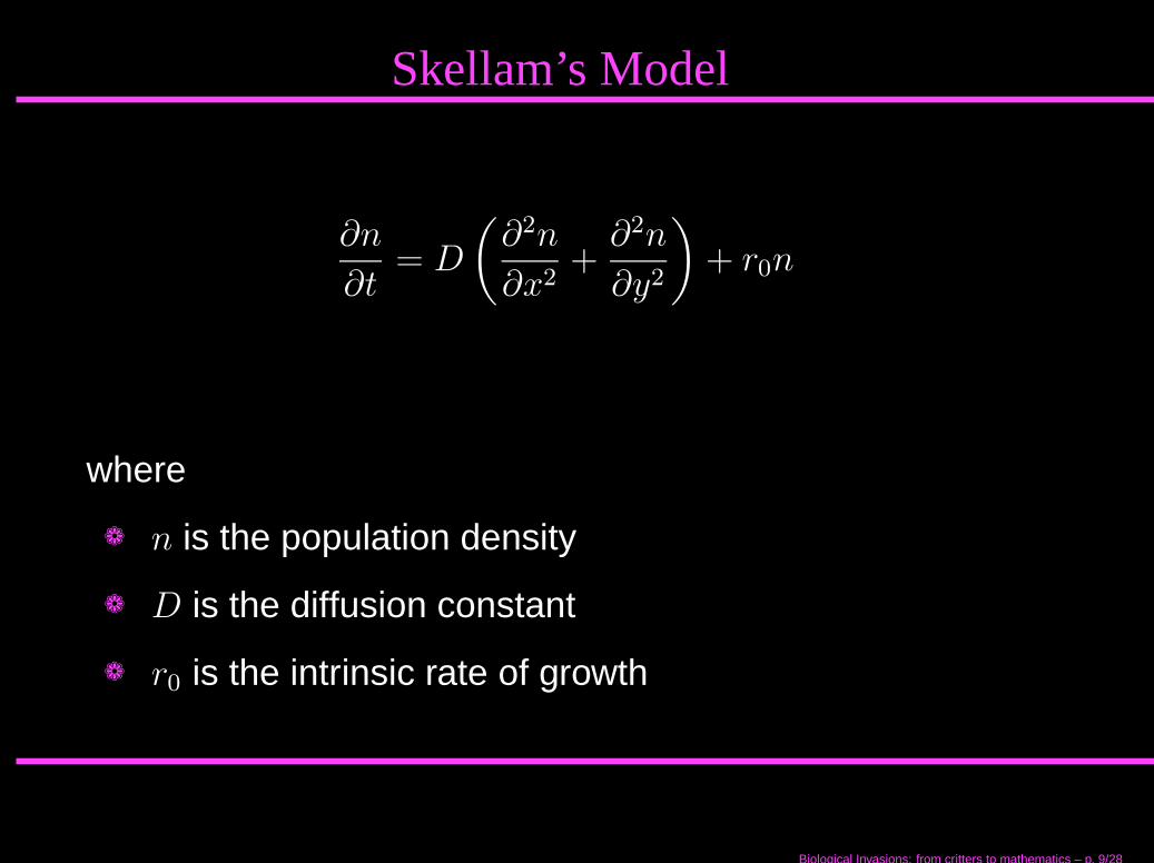
Skellam’s Model
∂n
∂t= D
(
∂2n
∂x2+
∂2n
∂y2
)
+ r0n
where
❁ n is the population density
❁ D is the diffusion constant
❁ r0 is the intrinsic rate of growth
Biological Invasions: from critters to mathematics – p. 9/28
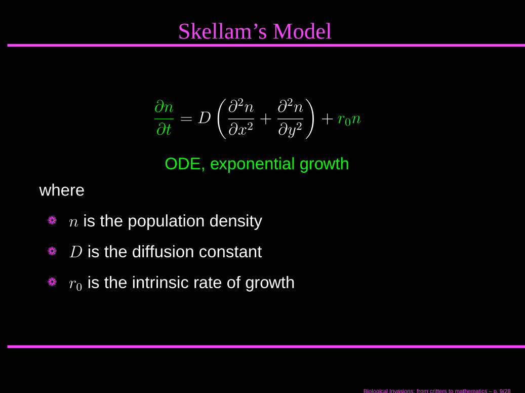
Skellam’s Model
∂n
∂t= D
(
∂2n
∂x2+
∂2n
∂y2
)
+ r0n
ODE, exponential growth
where
❁ n is the population density
❁ D is the diffusion constant
❁ r0 is the intrinsic rate of growth
Biological Invasions: from critters to mathematics – p. 9/28
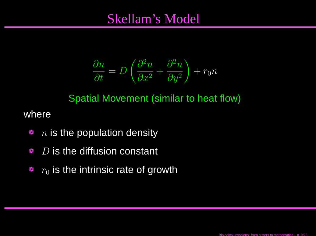
Skellam’s Model
∂n
∂t= D
(
∂2n
∂x2+
∂2n
∂y2
)
+ r0n
Spatial Movement (similar to heat flow)
where
❁ n is the population density
❁ D is the diffusion constant
❁ r0 is the intrinsic rate of growth
Biological Invasions: from critters to mathematics – p. 9/28
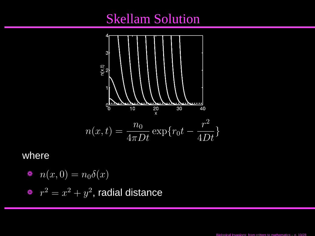
Skellam Solution
n(x, t) =n0
4πDtexp{r0t −
r2
4Dt}
where
❁ n(x, 0) = n0δ(x)
❁ r2 = x2 + y2, radial distance
Biological Invasions: from critters to mathematics – p. 10/28
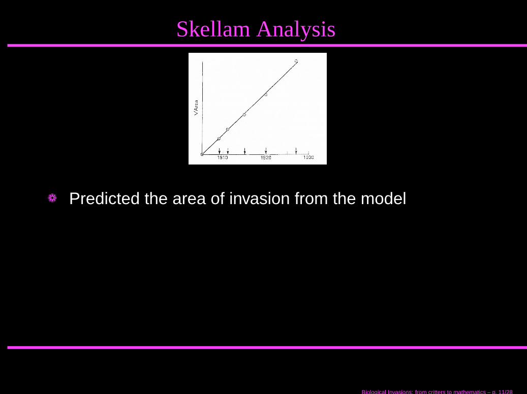
Skellam Analysis
❁ Predicted the area of invasion from the model
❁ Estimated the area from the Ulbrich map
Biological Invasions: from critters to mathematics – p. 11/28
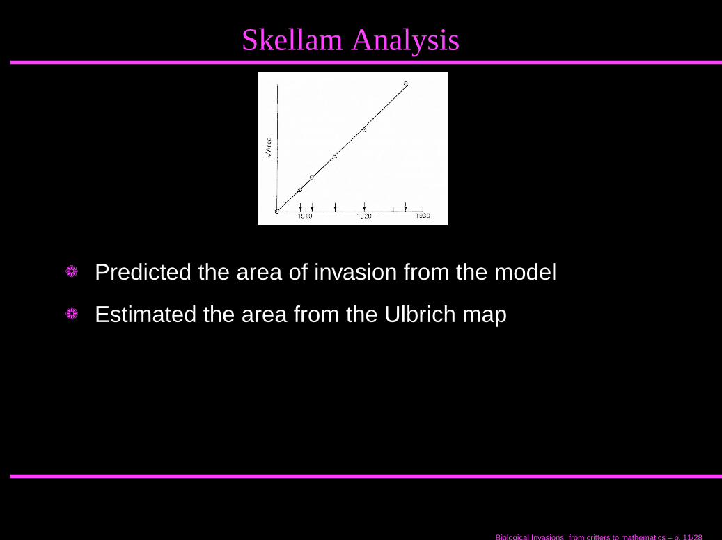
Skellam Analysis
❁ Predicted the area of invasion from the model
❁ Estimated the area from the Ulbrich map
Biological Invasions: from critters to mathematics – p. 11/28

Skellam Model
❁ Growth and dispersal are continuous
❁ Movement is a random diffusion process
Biological Invasions: from critters to mathematics – p. 12/28

Skellam Model
❁ Growth and dispersal are continuous
❁ Movement is a random diffusion process
Biological Invasions: from critters to mathematics – p. 12/28
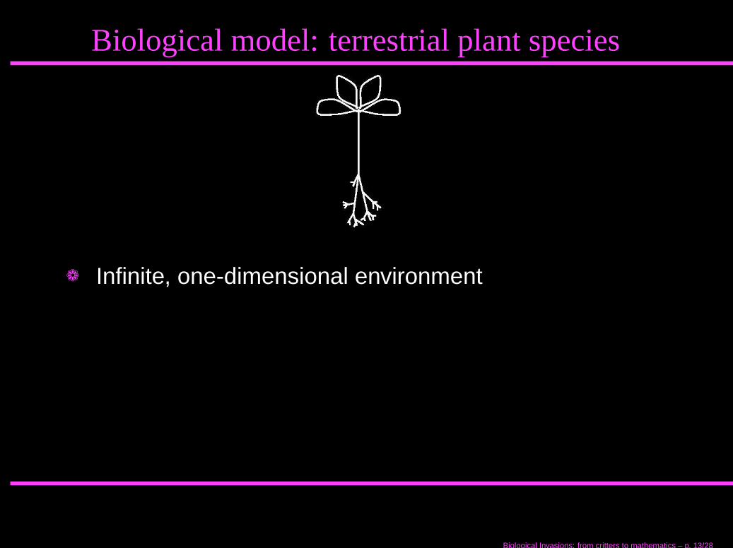
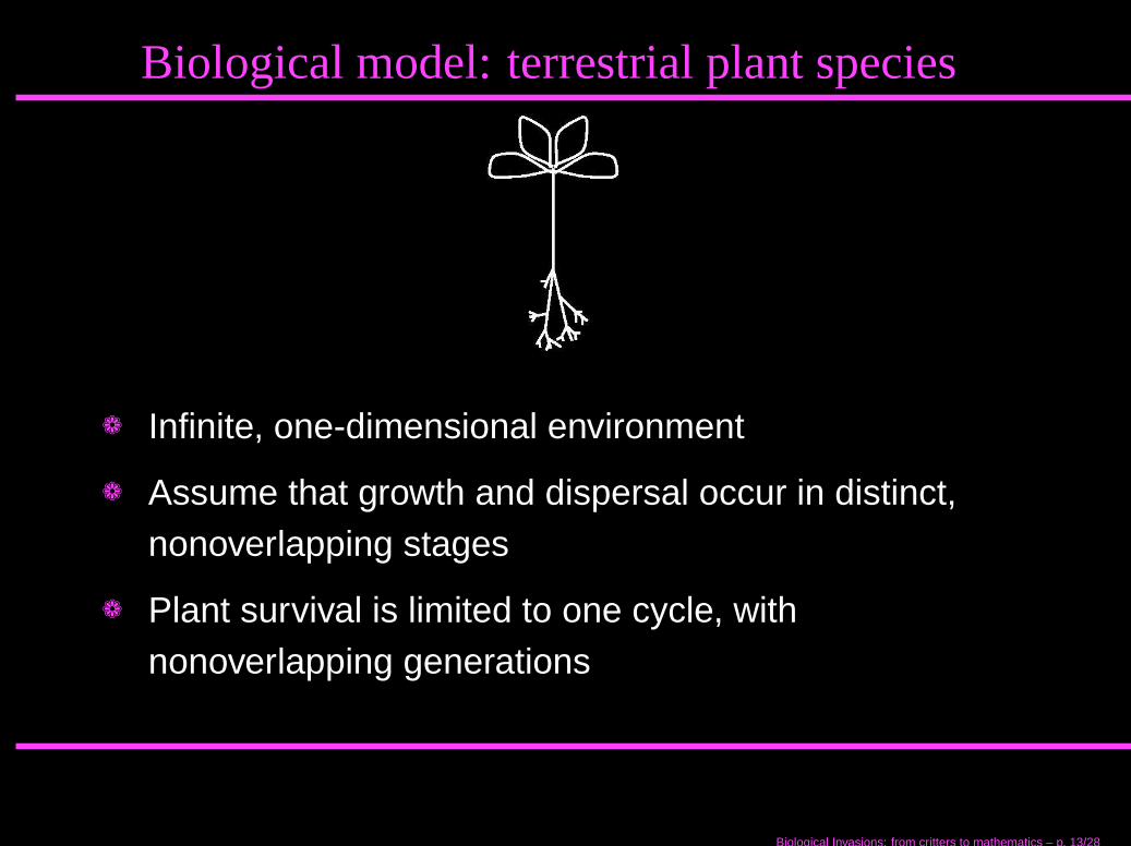
Biological model: terrestrial plant species
❁ Infinite, one-dimensional environment
❁ Assume that growth and dispersal occur in distinct,nonoverlapping stages
❁ Plant survival is limited to one cycle, withnonoverlapping generations
Biological Invasions: from critters to mathematics – p. 13/28
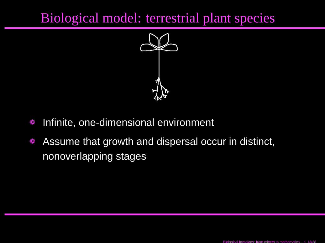
Biological model: terrestrial plant species
❁ Infinite, one-dimensional environment
❁ Assume that growth and dispersal occur in distinct,nonoverlapping stages
❁ Plant survival is limited to one cycle, withnonoverlapping generations
Biological Invasions: from critters to mathematics – p. 13/28
Biological model: terrestrial plant species
❁ Infinite, one-dimensional environment
❁ Assume that growth and dispersal occur in distinct,nonoverlapping stages
❁ Plant survival is limited to one cycle, withnonoverlapping generations
Biological Invasions: from critters to mathematics – p. 13/28
Mathematical model
Integrodifference equation (IDE) model for the populationdensity
Nτ+1(x) =
∫
+∞
−∞
f(Nτ (y); y)k(x, y)dy
where
❁ Nτ (x) is the population density
❁ f is the nonlinear growth function
❁ k(x, y) dispersal kernel
Biological Invasions: from critters to mathematics – p. 14/28
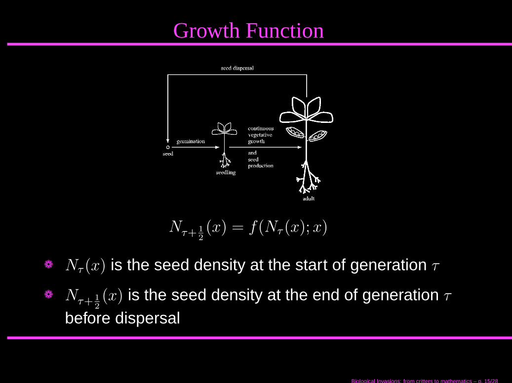
Growth Function
Nτ+1
2
(x) = f(Nτ (x); x)
❁ Nτ (x) is the seed density at the start of generation τ
❁ Nτ+1
2
(x) is the seed density at the end of generation τ
before dispersal
Biological Invasions: from critters to mathematics – p. 15/28

Growth Function example
Beverton-Holt stock-recruitment curve
f(N) =r0N
1 + [(r0 − 1)N ]
where r0 is the per capita reproductive ratio
r0 = 2.0
Biological Invasions: from critters to mathematics – p. 16/28
Dispersal Kernel
❁ k(x, y) is a pdf for a seed released from a location y
being deposited at a location x∫
+∞
−∞
k(x, y)dx = 1
❁ The IDE is the sum of all seeds dispersed to x∫
+∞
−∞
Nτ+1
2
(y)k(x, y)dy
Biological Invasions: from critters to mathematics – p. 17/28
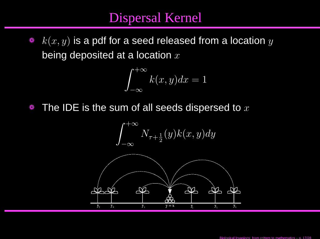
Dispersal Kernel
❁ k(x, y) is a pdf for a seed released from a location y
being deposited at a location x∫
+∞
−∞
k(x, y)dx = 1
❁ The IDE is the sum of all seeds dispersed to x∫
+∞
−∞
Nτ+1
2
(y)k(x, y)dy
Biological Invasions: from critters to mathematics – p. 17/28
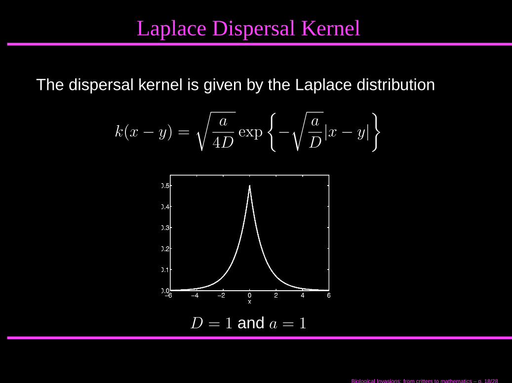
Laplace Dispersal Kernel
The dispersal kernel is given by the Laplace distribution
k(x − y) =
√
a
4Dexp
{
−
√
a
D|x − y|
}
D = 1 and a = 1
Biological Invasions: from critters to mathematics – p. 18/28
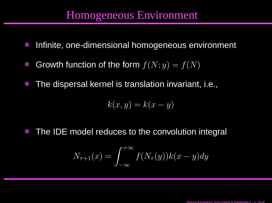
Homogeneous Environment
❁ Infinite, one-dimensional homogeneous environment
❁ Growth function of the form f(N ; y) = f(N)
❁ The dispersal kernel is translation invariant, i.e.,
k(x, y) = k(x − y)
❁ The IDE model reduces to the convolution integral
Nτ+1(x) =
∫
+∞
−∞
f(Nτ (y))k(x − y)dy
Biological Invasions: from critters to mathematics – p. 19/28

Homogeneous Environment
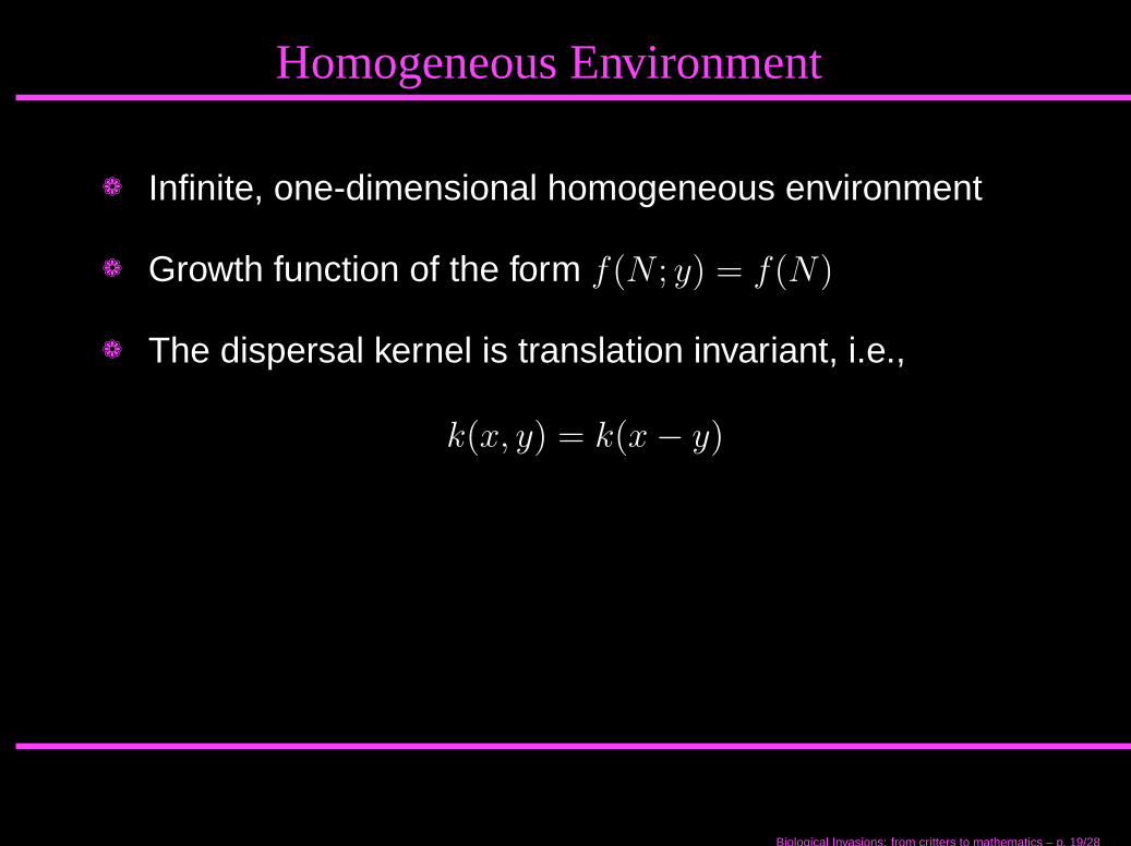
❁ Infinite, one-dimensional homogeneous environment
❁ Growth function of the form f(N ; y) = f(N)
❁ The dispersal kernel is translation invariant, i.e.,
k(x, y) = k(x − y)
❁ The IDE model reduces to the convolution integral
Nτ+1(x) =
∫
+∞
−∞
f(Nτ (y))k(x − y)dy
Biological Invasions: from critters to mathematics – p. 19/28
Homogeneous Environment
❁ Infinite, one-dimensional homogeneous environment
❁ Growth function of the form f(N ; y) = f(N)
❁ The dispersal kernel is translation invariant, i.e.,
k(x, y) = k(x − y)
❁ The IDE model reduces to the convolution integral
Nτ+1(x) =
∫
+∞
−∞
f(Nτ (y))k(x − y)dy
Biological Invasions: from critters to mathematics – p. 19/28
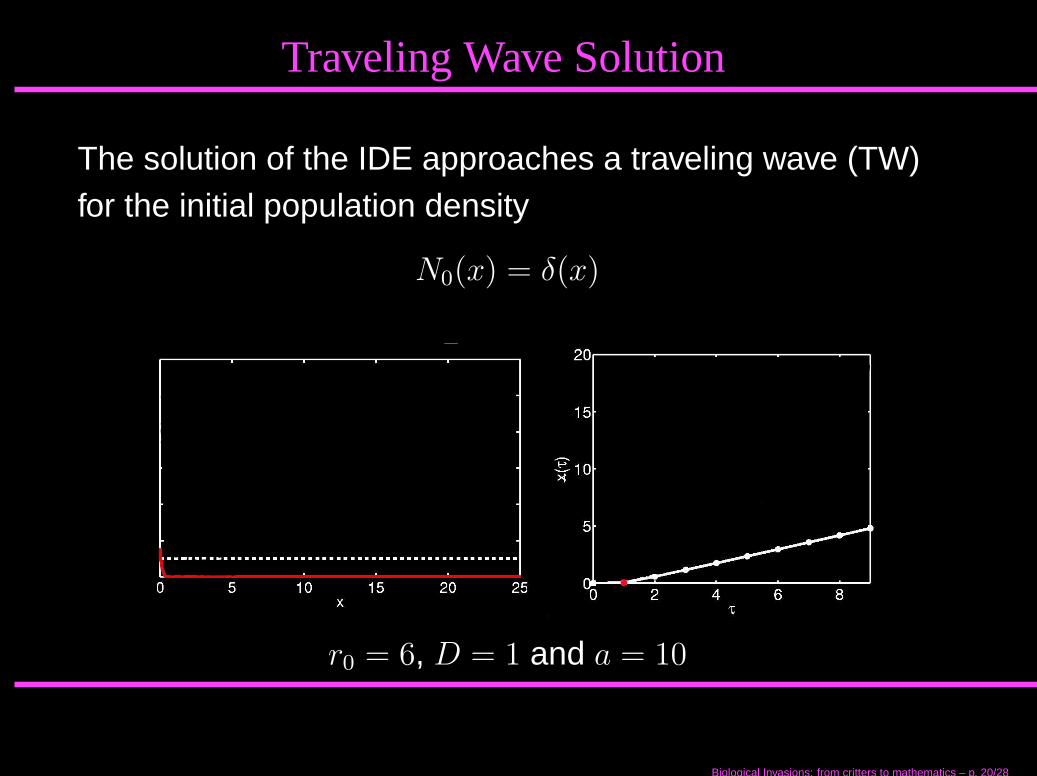
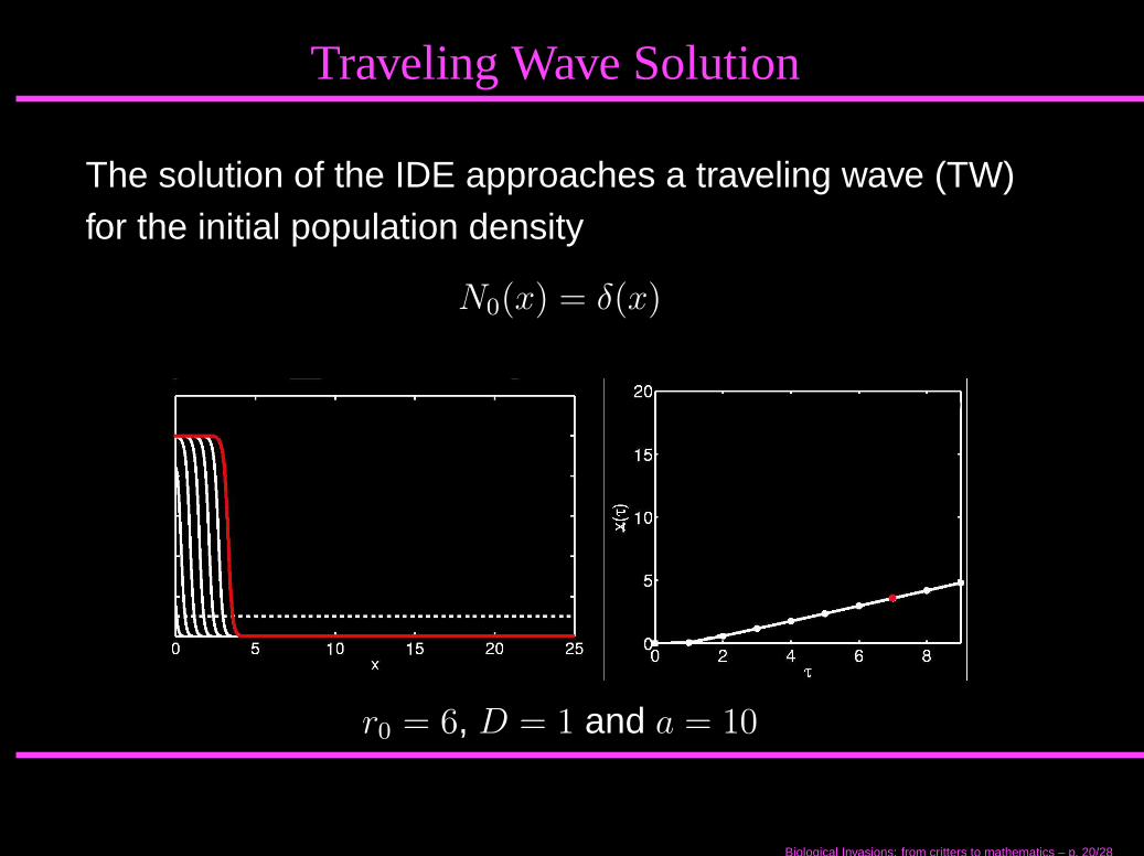
Traveling Wave Solution
The solution of the IDE approaches a traveling wave (TW)for the initial population density
N0(x) = δ(x)
r0 = 6, D = 1 and a = 10
Biological Invasions: from critters to mathematics – p. 20/28
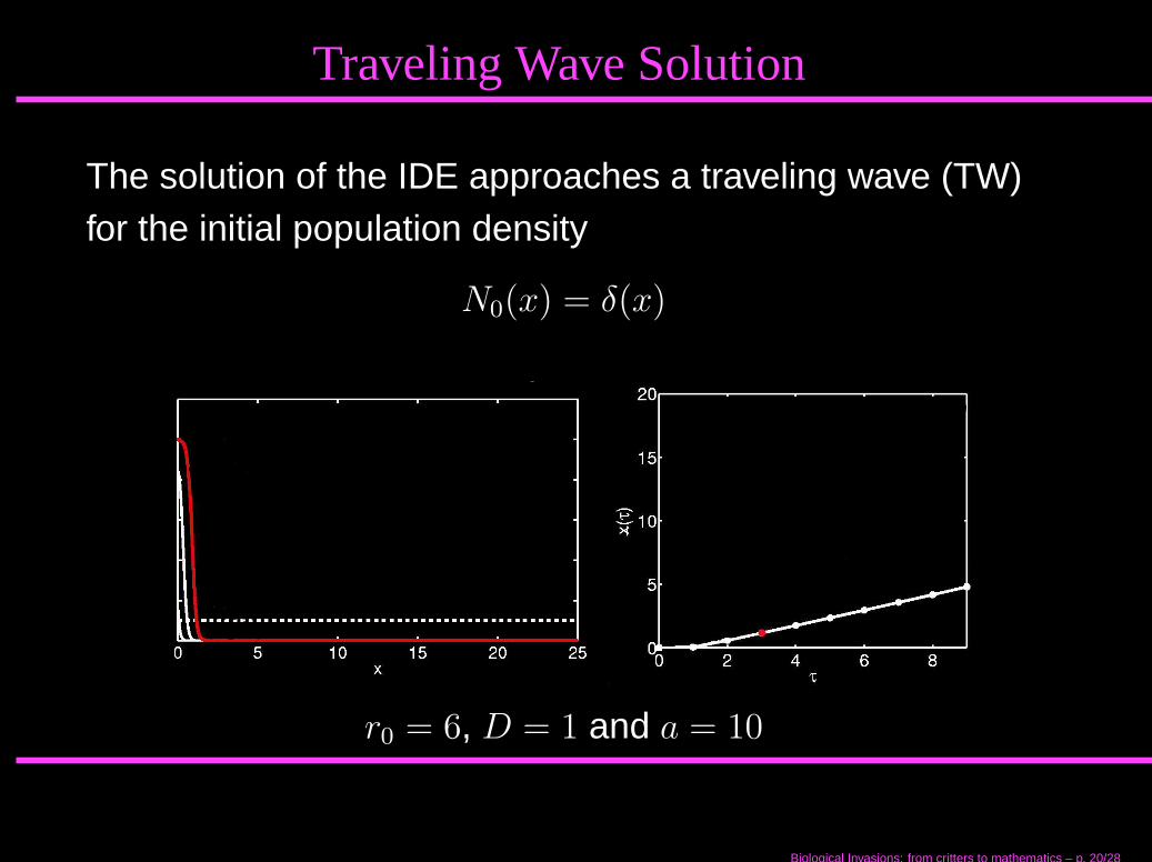
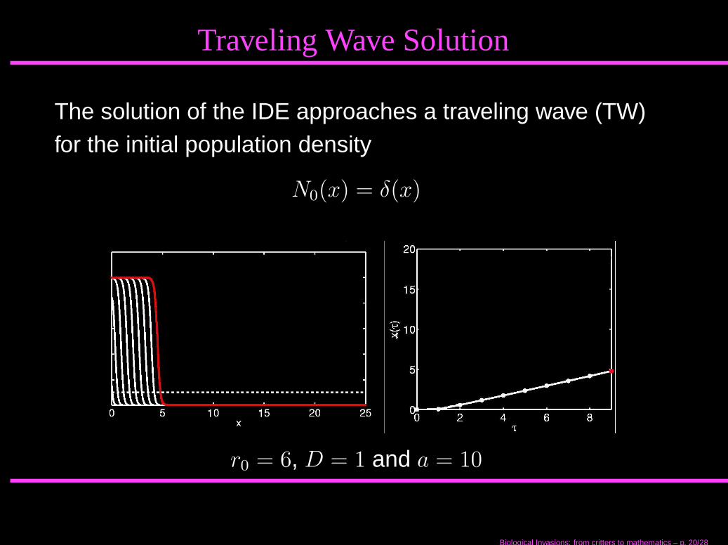
Traveling Wave Solution
The solution of the IDE approaches a traveling wave (TW)for the initial population density
N0(x) = δ(x)
r0 = 6, D = 1 and a = 10
Biological Invasions: from critters to mathematics – p. 20/28
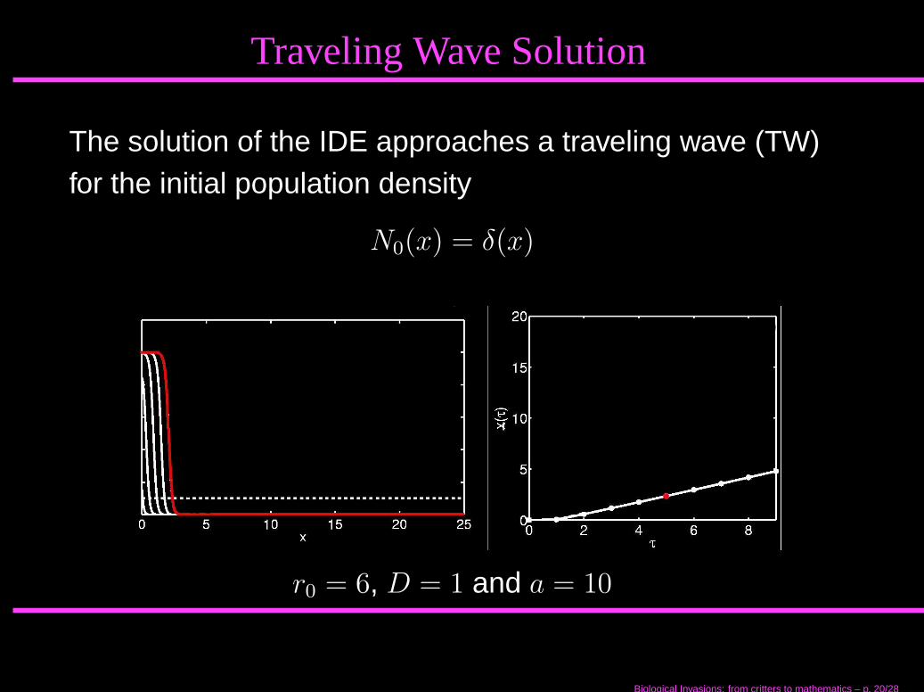
Traveling Wave Solution
The solution of the IDE approaches a traveling wave (TW)for the initial population density
N0(x) = δ(x)
r0 = 6, D = 1 and a = 10
Biological Invasions: from critters to mathematics – p. 20/28
Traveling Wave Solution
The solution of the IDE approaches a traveling wave (TW)for the initial population density
N0(x) = δ(x)
r0 = 6, D = 1 and a = 10
Biological Invasions: from critters to mathematics – p. 20/28
Traveling Wave Solution
The solution of the IDE approaches a traveling wave (TW)for the initial population density
N0(x) = δ(x)
r0 = 6, D = 1 and a = 10
Biological Invasions: from critters to mathematics – p. 20/28
Traveling Wave Results
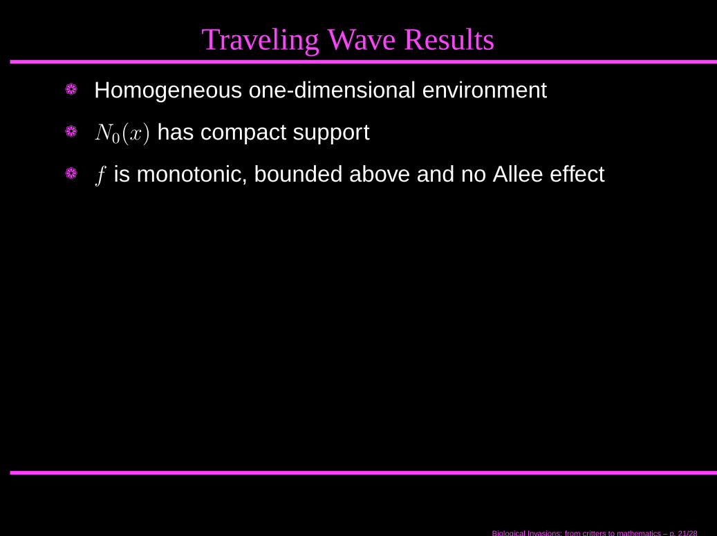
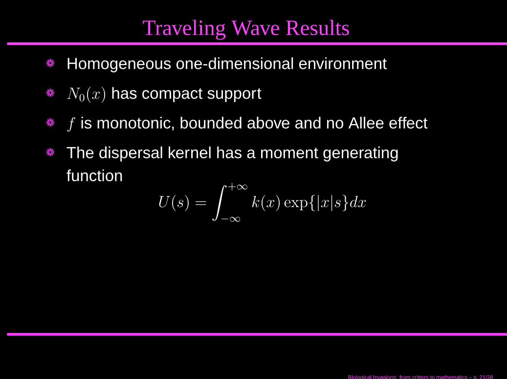
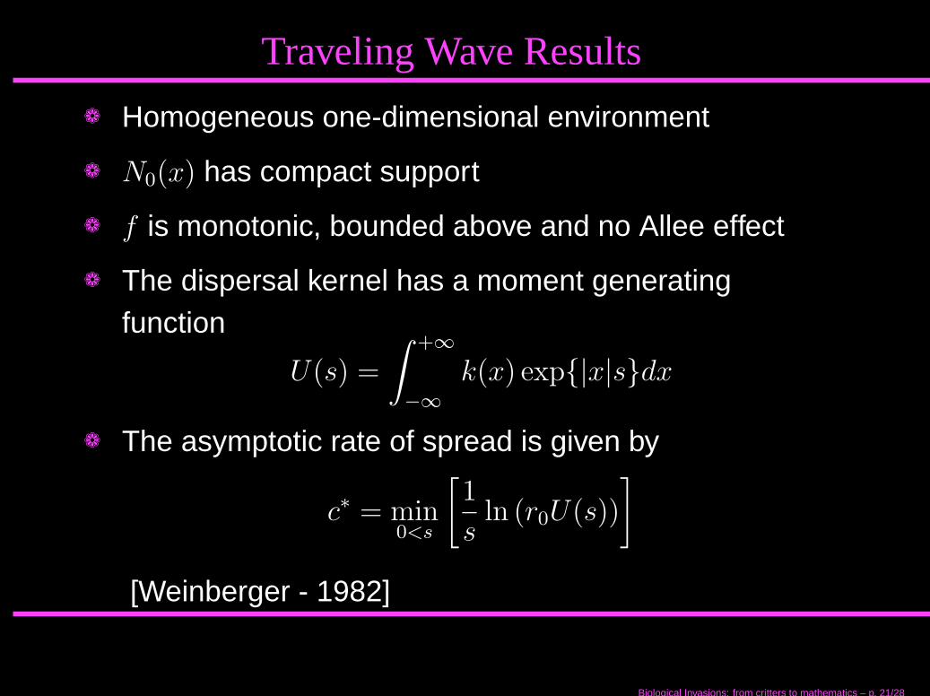
❁ Homogeneous one-dimensional environment
❁ N0(x) has compact support
❁ f is monotonic, bounded above and no Allee effect
❁ The dispersal kernel has a moment generatingfunction
U(s) =
∫
+∞
−∞
k(x) exp{|x|s}dx
❁ The asymptotic rate of spread is given by
c∗ = min0<s
[
1
sln (r0U(s))
]
[Weinberger - 1982]
Biological Invasions: from critters to mathematics – p. 21/28
Traveling Wave Results
❁ Homogeneous one-dimensional environment
❁ N0(x) has compact support
❁ f is monotonic, bounded above and no Allee effect
❁ The dispersal kernel has a moment generatingfunction
U(s) =
∫
+∞
−∞
k(x) exp{|x|s}dx
❁ The asymptotic rate of spread is given by
c∗ = min0<s
[
1
sln (r0U(s))
]
[Weinberger - 1982]
Biological Invasions: from critters to mathematics – p. 21/28
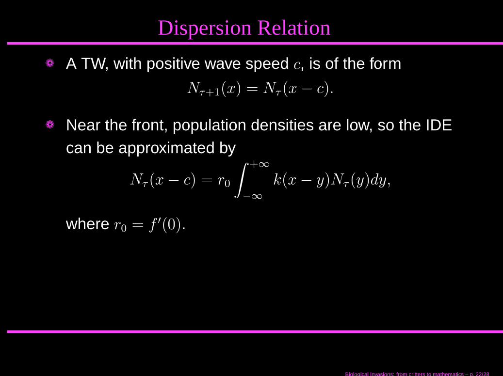
Dispersion Relation
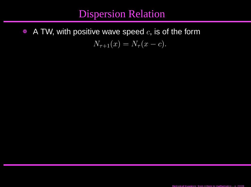
❁ A TW, with positive wave speed c, is of the form
Nτ+1(x) = Nτ (x − c).
❁ Near the front, population densities are low, so the IDEcan be approximated by
Nτ (x − c) = r0
∫
+∞
−∞
k(x − y)Nτ (y)dy,
where r0 = f ′(0).❁ TW ansatz: near the leading edge of the wave
Nτ (x) ∝ e−sx
for s > 0.
Biological Invasions: from critters to mathematics – p. 22/28
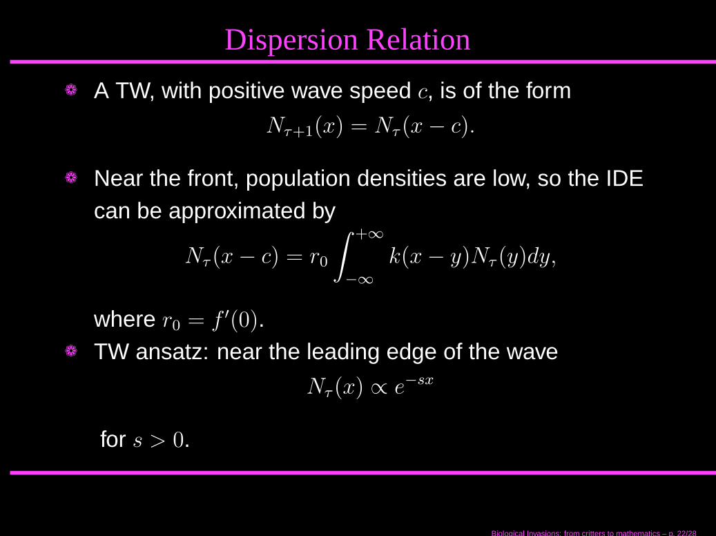
Dispersion Relation
❁ A TW, with positive wave speed c, is of the form
Nτ+1(x) = Nτ (x − c).
❁ Near the front, population densities are low, so the IDEcan be approximated by
Nτ (x − c) = r0
∫
+∞
−∞
k(x − y)Nτ (y)dy,
where r0 = f ′(0).
❁ TW ansatz: near the leading edge of the wave
Nτ (x) ∝ e−sx
for s > 0.
Biological Invasions: from critters to mathematics – p. 22/28
Dispersion Relation
❁ A TW, with positive wave speed c, is of the form
Nτ+1(x) = Nτ (x − c).
❁ Near the front, population densities are low, so the IDEcan be approximated by
Nτ (x − c) = r0
∫
+∞
−∞
k(x − y)Nτ (y)dy,
where r0 = f ′(0).❁ TW ansatz: near the leading edge of the wave
Nτ (x) ∝ e−sx
for s > 0.
Biological Invasions: from critters to mathematics – p. 22/28
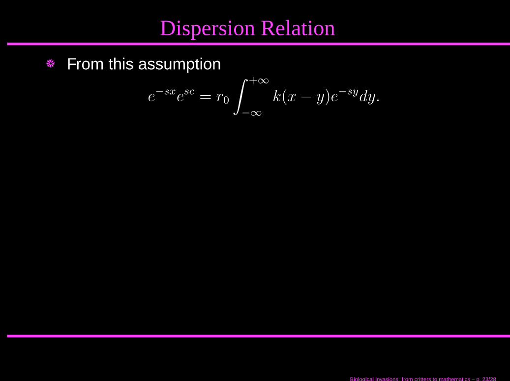
Dispersion Relation
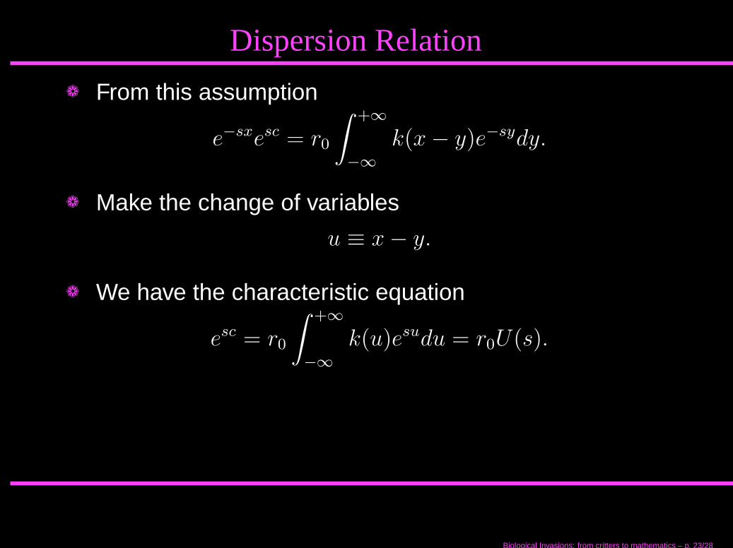
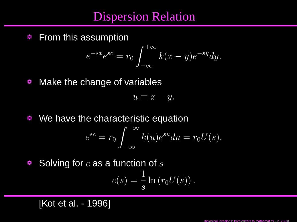
❁ From this assumption
e−sxesc = r0
∫
+∞
−∞
k(x − y)e−sydy.
❁ Make the change of variables
u ≡ x − y.
❁ We have the characteristic equation
esc = r0
∫
+∞
−∞
k(u)esudu = r0U(s).
❁ Solving for c as a function of s
c(s) =1
sln (r0U(s)) .
[Kot et al. - 1996]
Biological Invasions: from critters to mathematics – p. 23/28
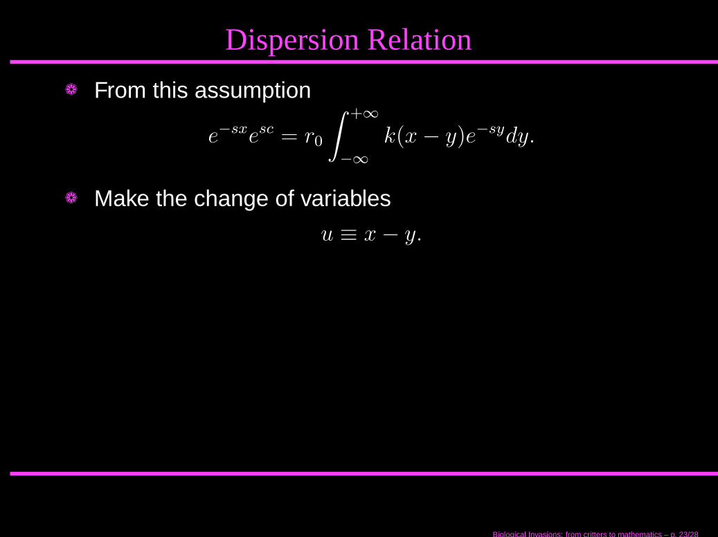
Dispersion Relation
❁ From this assumption
e−sxesc = r0
∫
+∞
−∞
k(x − y)e−sydy.
❁ Make the change of variables
u ≡ x − y.
❁ We have the characteristic equation
esc = r0
∫
+∞
−∞
k(u)esudu = r0U(s).
❁ Solving for c as a function of s
c(s) =1
sln (r0U(s)) .
[Kot et al. - 1996]
Biological Invasions: from critters to mathematics – p. 23/28
Laplace Kernel Dispersion Relation
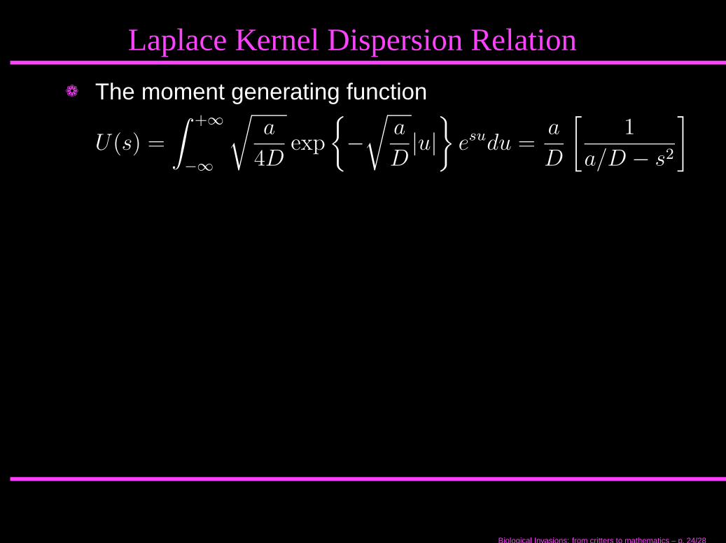
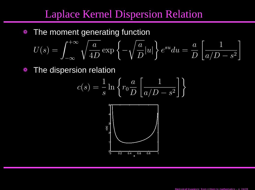
❁ The moment generating function
U(s) =
∫
+∞
−∞
√
a
4Dexp
{
−
√
a
D|u|
}
esudu =a
D
[
1
a/D − s2
]
❁ The dispersion relation
c(s) =1
sln
{
r0
a
D
[
1
a/D − s2
]}
Biological Invasions: from critters to mathematics – p. 24/28
Laplace Kernel Dispersion Relation
❁ The moment generating function
U(s) =
∫
+∞
−∞
√
a
4Dexp
{
−
√
a
D|u|
}
esudu =a
D
[
1
a/D − s2
]
❁ The dispersion relation
c(s) =1
sln
{
r0
a
D
[
1
a/D − s2
]}
Biological Invasions: from critters to mathematics – p. 24/28
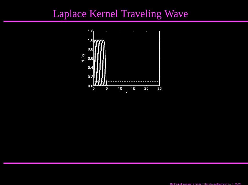
Laplace Kernel Traveling Wave
Biological Invasions: from critters to mathematics – p. 25/28

Laplace Kernel Traveling Wave
Biological Invasions: from critters to mathematics – p. 25/28
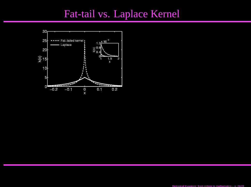
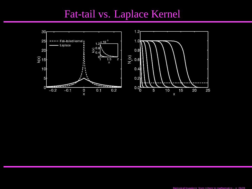
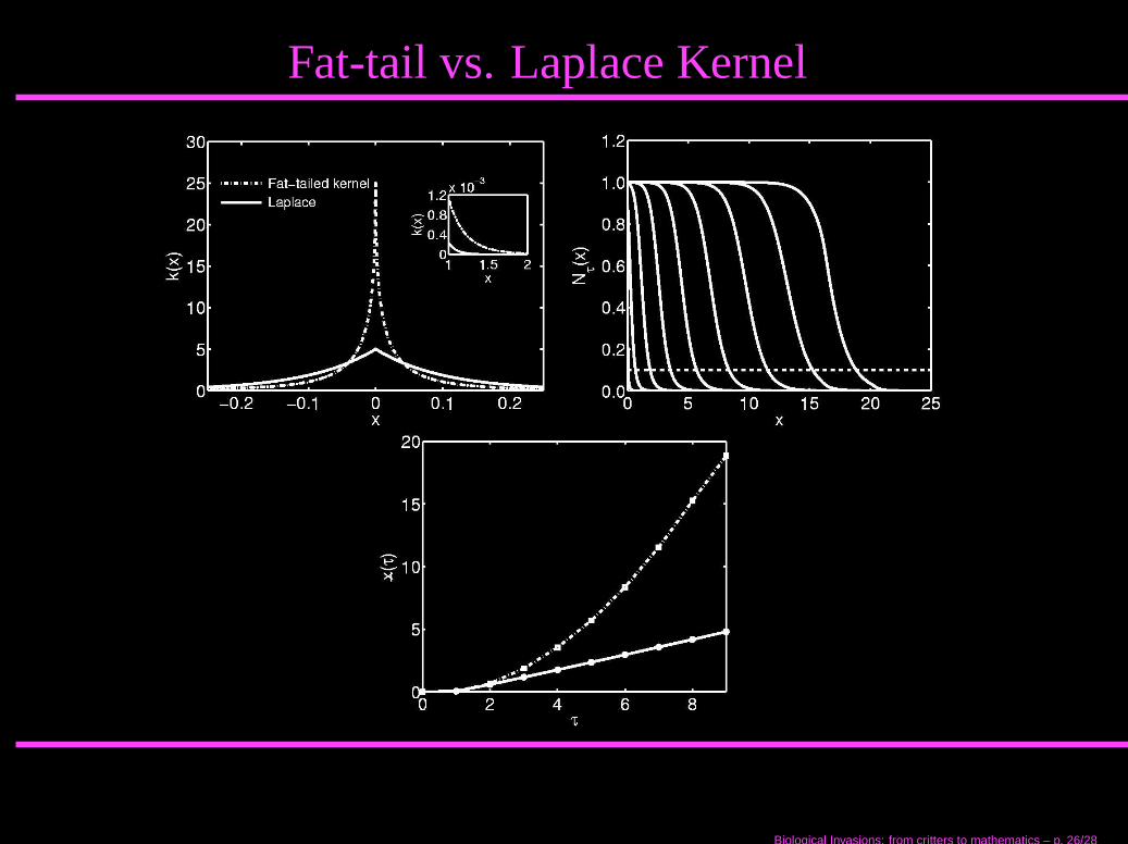
Fat-tail vs. Laplace Kernel
Biological Invasions: from critters to mathematics – p. 26/28
Fat-tail vs. Laplace Kernel
Biological Invasions: from critters to mathematics – p. 26/28
Fat-tail vs. Laplace Kernel
Biological Invasions: from critters to mathematics – p. 26/28
Summary
❁ Many aspects of biological invasions to consider
❁ Homogeneous vs. heterogeneous environment,1-d vs. 2-d, ...
❁ IDE model sensitive to shape of the dispersal kernel
❁ Models for non-discrete time, i.e., integrodifferentialequations?
Biological Invasions: from critters to mathematics – p. 27/28
References❁ C. S. Elton, The Ecology of Invasions by Animals and Plants,
Chicago University Press, 2000.
❁ M. Williamson, Biological Invasions, Chapman and Hall,Population and Community Biology Series (No. 15), 1997.
❁ N. Shigesada and K. Kawasaki, Biological Invasions: Theory andPractice, Oxford University Press, Oxford Series in Ecology andEvolution, 1997.
❁ M. Kot, M. A. Lewis and P. van den Driessche, Dispersal data andthe spread of invading organisms, Ecology, 77 (1996), pp.2027-2042.
❁ H. F. Weinberger, Long-time behavior of a class of biologicalmodels, SIAM Journal of Mathematical Analysis, 3 (1982), pp.353-396
Biological Invasions: from critters to mathematics – p. 28/28