biology extended essay the effects of … · the effects of electromagnetic fields in the...

1

BIOLOGY EXTENDED ESSAY

THE EFFECTS OF ELECTROMAGNETIC FIELDS IN THE RESISTANCE OF A PLANT TO CHILING TEMPERATURES

TROYA ÇAĞIL KÖYLÜ

D1129-045

WORD COUNT: 3925

ADVISOR: ÜMİT YAŞATÜRK

ANKARA

2010

2

ABSTRACT

In this study, the effects of E.F. in 10 and 40 minutes periods every day, in midday

and normal room conditions to the plant Cactus suculent was investigated. The E.F. was

applied by two plates that are charged by negative and positive charges. After the E.F.

application, the plants are carried into chilling colds (-17 ⁰C, 15/21 light/dark), other plants

carried to normal conditions . Both plant groups are marked with numbers. All plant groups

were exposed to cold 40 minutes after E.F. application. All trials( ten times) are repeated and

their results are analysed statistically.

This experiment is carried in June-July-August-September months for 105 days in

2009.

10 minutes of E.F. has no differences with the control group in normal conditions but

it was observed that they have more lifetime. However, it was observed that 40 minutes of

E.F. has inhibitory effects.

Keywords: Electrical field, cactus suculent, , cold acclimation, chilling resistance

Word Count: 3925

3

THANKS

This essay has been written in TED Ankara College Private High School. The

experiments had been carried in house area.

I want to thank my adviser teacher whose name is Ümit YAŞATÜRK (TED Ankara

College Foundation Private High School biology department) who built up my academic

work.

Finally, I want to thank my family; Meltem Keskin Köylü, helped me in statistical

analysis and Murat Köylü in structural form and thanks again for their motivation and care.

Troya Çağıl KÖYLÜ

January 2010

4

CONTENS

ABSTRACT..................................................................................................................iii

THANKS.......................................................................................................................v

SYMBOLIZES and ABBREVIATION INDEX............................................................vİ

ILLUSTRATIONS INDEX.......................................................................................... vii

TABLES INDEX .........................................................................................................viii

1.INTRODUCTION .................................................................................................... 1

2. MATERIALS AND METHODS............................................................................... 10

2.1. Materials…….……………………………………………………..………………….. 10

2.2. Methods.............................................................................................................. 10

2.2.1.Plantation and breeding of the plants............................................................... 10

2.2.2. Sampling …………………………………………………………………………… 11

2.3. Treating the plants........................................................................................... 12

2.3. Analysis Teqniques ……….. .............................................................................. 17

3.THE DATA OF THE EXPERIMENT...................................................................... 18

3.1. Hypothesis, analysis and evaluation …….......................................................... 18

4. RESULTS AND SUGGESTIONS………………………….. ……………………… 27

4.1. The Effects of Electromagnetical Field..…..……………………………………… 27

4.2. The Effects of Cold and E.F. Application...…………..…………………………… 28

5. STUDY LIMITS AND CHANCES OF MISTAKES ……………………………....... 30

BIBLIOGRAPHY ………………………………………………………………………….. 31

5

SYMBOLIZES AND STRINGS ATTACHED INDEX

ºC : Celsius derecesi

min : Minute

g : Gram

cm : Cantimetre

ml : Millimetre

sec : Second

List of Abbreviations

E.F. : Electromagnetic Field

A : General Control

A1 : 10dk E.F. application + cold

A2 : 40dk E.F. application + cold

B : General Control

B1 : no application of e.f. + cold

B2 : no application of e.f.+ cold

AC : Alternative Current

DC : Direct Current

ELC. APL. Electric Application

6

ILLUSTRATION INDEX

Illustration 1.1. The diagram of effects of electrical fields from the high voltage lines to its surroundings that was observed by some researchers …………………........................................................................................................

3

Illustration 1.2. The diagram showing sensitive plants responses to the process of undergoin getting cold’ temperatures..………………………………………………

5

Illustration 2.1. the effection of cacti..……………………………………………….. 12

Illustration 2.2 Temperature changes …………………………… …………………. 15

Illustration 2.3.The living length of the plants ………………………….……………

15

Illustration 2.4. the celcius variance graph ……………………………………………. 16

Illustration 2.5 The change of size in plants that are influenced and not influenced graph……………………………………………………………………………………….

17

Illustration 3.1 Experiment photos ……………………………………………………… 26

7

TABLES INDEX

Table 2.1 The height and width of young cacti that are carried to little pots …….. 11

Table 2.2. The affectance periods of the electromagnetic field …….……....…… 13

Table 2.3. The differences in the means of cold and electromagnetical affectance between plant groups ………………..………..…………..……………....................

14

Table 2.4 The living periods of plant groups (1=live, 0=dead)…………………… 14

Table 3.1. Case processing summary …….. ……………………………………… 18

Table 3.2. 10 min ELC. APL. * b1 Crosstabulation ………………………………. 18

Table 3.3. Chi-Square Tests…………………………………………………………..

19

Table 3.4. Statistics …………………………………………………………………… 19

Table 3.5. 10min elc apl. (Electric Application)…………………………………… 20

Table 3.6. 40min elc apl. (Electric Application)…………………………………….

20

Table 3.7. B1 values …………………………………………………………………

20

Table 3.8. B2 values ………………………………………………………………….

20

Table 3.9. Oneway……………………………………………………………………. 21

Table 3.10. t-Test …………………………………………………………………. 23

Table 3.11. Frequency table ………………………………………………………….

24

Table 3.12. Descriptives …………………………………………………….. ……..

25

8

INTRODUCTION

All plants in the world are in the effect of the world’s magnetic and electrical

fields because the world features as a large bar magnet ( Nelson and Walker, 1961;

Takahashi, 1986; Watanabe and Yamashita, 1987; Maeda, 1993) and there is a

continuous electrical field between clouds and earth. ( Oomori, 1992) In the presence

of a thunder, the electrical field is enlarged very rapid (Ohanian, 1989) and normaly

negative charged soil is covered with positive charges thus the plants are effected

from this electrical field change.

By the way, it is well to explain some physical terms to make them clear; A

current passing through a wire creates an electrical field around it. The same area

can be also created by charging two aluminum plates with (+) and (-) charges. The

electric field direction is from (+) to (-). Electrical and magnetic fields are similar

physical forces in the means of their effects on living organisms although they are

different from each other. A magnet’s effected area is called the ‘magnetic field’ of

the magnet. The lines that are formed in the surrounding of the magnet are called

‘the magnetic field lines’ of the magnet. The direction of these lines are from north to

west. Low frequenced electromagnetic areas have lower frequences than 10⁵ Hz. As

this sources usually cover electrical transmission lines and some electrical devices,

they can be called ‘electrical fields’.( Kocaçalışkan, 2004)

It is reported that, all organisms including humans are effected from the

electrical field and the effects of electrical and magnetic fields on biologic systems is

9

an interesting field of study that can give important results.( Polk and Postow, 1995;

Kodali, 1996).

The main reason that plants are effected from the electrical fields is the

industrialism. In our modern and industral world, the electrical field in areas can vary

between 0 – 3 x 10⁶ V/m.( Benson, 1991) And there is many information missing of

the effects of electrical areas to living systems. Especially, there are not enough

studies about the long term exposure but it is known that values above 25 kV/m are

due to result in dangerous results.( Kocaçalışkan, 2004)

Today, the electric transmission is generally supplied with high voltaged lines.

These lines carry about 380 – 700 kV electrical energy. In this case, the electrical

field under the transmission lines are supposed to be 5 – 12 kV/m. The study of the

effects of this field on living organisms in that area is continuing.( Foster, 1996;

Koçyiğit, 2000)

In some studies about the security standards made in USA and Japan, the

upper limit of the electrical field between the high voltage lines is 3 kV/m. Although

under this level, no serious health problem was observed; above this level, it was

obseved that especially in blood cells, there were health problems observed in living

organisms.( Kocaçalışkan, 2004)

All biological systems consist of subsystems. To understand these systems

functions, effects of fields on biological solutions must be known. These liquids

include diversity of molecules. The transmission is changeable in these systems. By

this changes, the organisms’ life functions change.( Kocaçalışkan, 2004)

10

Illustration 1.1. – The diagram of effects of electrical fields from the high voltage lines to its surroundings that was observed by some researchers.( Şeker and Çerezci, 1991)

In the nature, the plant species that are living in an area is designated by the

natural selection that arises from the ecological circumstances of that area. As a

result, humans are creating artificial areas to breed plants that they need. In areas

that several factors affecting the plant growth, biotechnological ways are used aside

Ele

ctric

al fi

eld

(kv

/m)

1000

500

200

100

50

20

death of sample cells( d’Ambrosw Gann)

death of fruit flies( Solov’ev Watson)

temporary increase in metabolic activities in mice

( Hilmer, Rosenberg)

coronal damage in leaf ends( McKeek, Bankoske, Hodges, Rogers)

11

conventional ways. On the contrary however, preventing the damage of chiling

temperatures to plants is still an obstacle and to overcome that problem, the studies

about cold’s biological effects on plants that are resistable and irresistable to cold

must be enlarged.( Dumlupınar, 2000)

In our current knowledge, the plants can be classified in three groups on their

resistance to cold; sensitive, semi-sensitive, resistant. This grouping is made by

looking their surviving times without getting any damage and it is seen that there is a

‘getting cold’ limit temperature for every variations of plants. The resistance to cold

ability can even show differences in the same kind of plant.( Guy,1990) Plants’ ‘cold’

limit is based on the level of cold, exposure time, also the humidity of the

surrounding, the plant’s maturity, the sugar level in the structure of the plant, its cell

wall’s saturated fat rate and value, the soil’s nutriently value of saturation and the

plant’s ability to change its hormones.( Wang, 1982)

In the studies, it was seen that about the cold resistance of a plant, the effects

of biological and physyological cahanges are vital because it was also seen that,

there is a difference in resistance between the tissues of the plant and that factor

makes the subject impossible to be carried out by just genetical methods.( Guy,

1990)

12

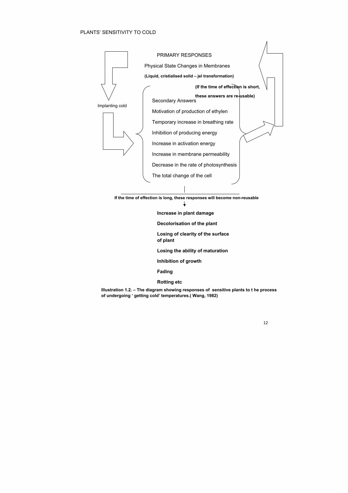
PLANTS’ SENSITIVITY TO COLD

PRIMARY RESPONSES

Physical State Changes in Membranes

(Liquid, cristialised solid – jel transformation)

Implanting cold Secondary Answers

Motivation of production of ethylen

Temporary increase in breathing rate

Inhibition of producing energy

Increase in activation energy

Increase in membrane permeability

Decrease in the rate of photosynthesis

The total change of the cell

If the time of effection is long, these responses will become non-reusable

Increase in plant damage

Decolorisation of the plant

Losing of clearity of the surface of plant

Losing the ability of maturation

Inhibition of growth

Fading

Rotting etc

(If the time of effection is short,

these answers are re-usable)

Illustration 1.2. – The diagram showing responses of sensitive plants to t he process of undergoing ‘ getting cold’ temperatures.( Wang, 1982)

13

In the plants that are influenced by chiling colds, the primary response is

observed to be changes in the membrane structures. Also, by the change of the

membrane structure in the plants that are sensitive to cold, the enzyme system is

influenced. Therefore, the enzyme activity is shown to be related with the membrane.

However, it is seen that there is no membranous change and enzyme activity change

in plants that are resistant to cold. (Raison et al., 1971)

The chiling temperatures have effects on a plants physical and biochemical

mechanisms alongside with their cell membranes. In the development of the

resistance, one important factor is the increase of the soluble amount of proteins.

The studies showed that, the resistance occurs from the synthesis of resistable

proteins.( Kocaçalışkan, 2004)

In the studies on this subject, it was seen that by the effect of cold, there are

many biochemical and physical changes occur; the positively and negatively external

effects on the resistance mechanism. The plants are not encountered by the galvanic

cold changes without the presence of frost. Usually, the heat decreases slowly. In

this process, the plant detects the decreasing heat and starts to react. Although this

process is not very vital to resistant plants, the sensitive plants need this biochemical

and physical changes. The exposure period is even so important for this sensitive

plants. If this period is not sufficient for the plant to react, crucial damages will occur.(

Dumlupınar, 2000)

In this process, to prevent the cold stress on the plant, some regulating

substances are used and some important results were obtained.( Waldmen, 1975;

Young and Lee, 1979; Abromeit, 1992; Dumlupınar, 2000) But the reality is that,

these studies are based on agricultural plants and the aim is to protect the plants

from human consume in their natural areas. But many science authorities are taking

14

this usage suspicional. The usage of this regulating substances is considered to

effect the human health. In addition, there were many knowledge gained about the

plants resistance but there is almost no researches about the electrical field effects

on plants resistance to cold.

In this study, the effects of an electrical field which is a physical force to the

plants resistance to the chiling temperatures will be elaborated. To do that, we need

to use a plant that is sensitive to cold and the easiest one to find is the cactus plant.

Plant:

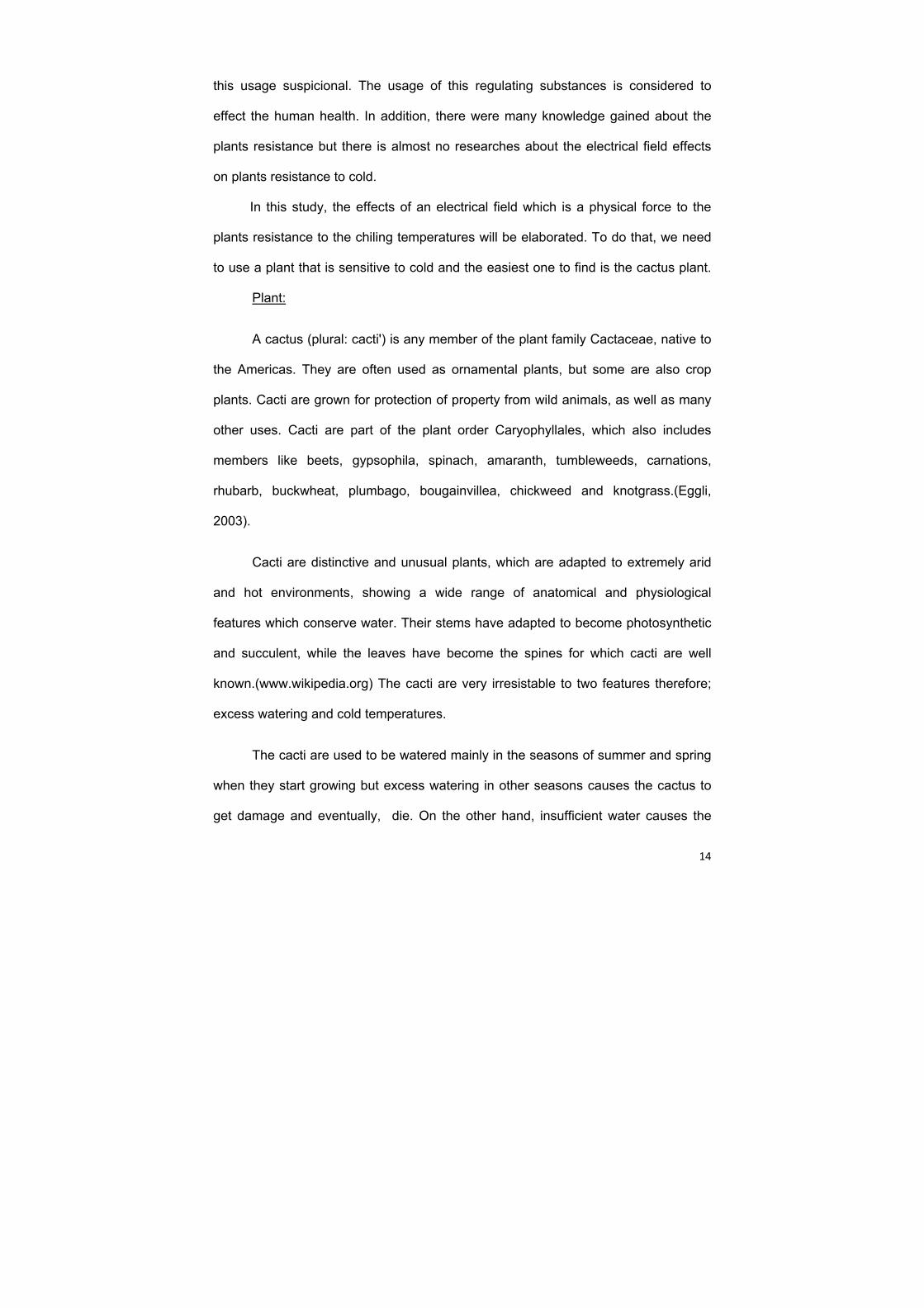
A cactus (plural: cacti') is any member of the plant family Cactaceae, native to

the Americas. They are often used as ornamental plants, but some are also crop

plants. Cacti are grown for protection of property from wild animals, as well as many

other uses. Cacti are part of the plant order Caryophyllales, which also includes

members like beets, gypsophila, spinach, amaranth, tumbleweeds, carnations,

rhubarb, buckwheat, plumbago, bougainvillea, chickweed and knotgrass.(Eggli,

2003).

Cacti are distinctive and unusual plants, which are adapted to extremely arid

and hot environments, showing a wide range of anatomical and physiological

features which conserve water. Their stems have adapted to become photosynthetic

and succulent, while the leaves have become the spines for which cacti are well

known.(www.wikipedia.org) The cacti are very irresistable to two features therefore;

excess watering and cold temperatures.

The cacti are used to be watered mainly in the seasons of summer and spring

when they start growing but excess watering in other seasons causes the cactus to

get damage and eventually, die. On the other hand, insufficient water causes the

15

cactus to enter a sleep mode that doesn’t give permenant damages to cactus

afterwards.

In my study, the cacti are plants that are very resistable to very high

temperatures but their minimum average living temperature is 0⁰C.(by the way, their

optimum growing temperature is 16⁰C) There are some cactus species that can

resist up to -15⁰C but they are very rare. In winter, the cacti enter a sleep mode to

survive winter conditions but if they are effected by chiling temperatures for a long

period of time, they start to get damage. At first, wounds start to appear on the mid-

section and then, by the damage of this section, the plant collapses.

History

There weren’t any studies made before 1960s except some exceptions. Until

then, there were many studies have been made. Some researchers studied about

the effects of electrical field on the environment.(Navy sponsored ELF Biological and

Ecological Research Summary, 1977) And some researchers studied about the

effect of the field on growing and maturing process.(Murr, 1963; Barthony, 1969). It is

therefore stated that the electrical field has an influence on the cell reproduction.

Lebedev(1930) has used low frequenced, short-term elecrical waves on a

plant and observed that growing is 20-45% more compared to the control

group.(Nelson, 2000)

Lazarenko and Gorbatovskaya(1966) observed that the adaptation gained by

the effected plants can be transferred up to the 3rd generations.

On the other hand, by some high voltage applications by Solov’ev(1967), the

effect on the living organisms are observed to be deadly.

16

There are some studies continuing about speeding or delaying the growth of

plants.(Bachman and Reichmanis 1973; Murr 1963, 64, 65, 66) In some studies, it is

observed that the electrical field causes inhibitory effects.(Murr, 1965; Hart and

Schottenfeld, 1979).

There are also some knowledge that the electrical or magnetic applications

increase the rate of the enzyme that cause an increase of the plant’s metabolic

activities.(Murr, 1965; Jia Ming, 1988; Kurinobu and Okazaki, 1995)

Azin and Izakov(1995) observed that the efficiency in agriculture has

increased 15-20% when they applicated electrical field on the seeds.(Nelson, 2000)

With related to our study, when plants are exposed to cold temperatures, it is

seen that they give primary responses and when the exposing time of chiling

temperatures is long, they give secondary responses(Pantastico et al., 1967; Eaks,

1980) and it was stated that the secondary responses are good parameters of

obtaining the cold heat damage on the plant.(Eaks,1980)

When a plant is effected by a cold temperature, it is observed that the primary

response is a change on the membrane structure of their cell and also enzyme

activity is related with the components of the cell membrane.

When a study was made on both sensitive and insensitive plants to cold, it

was observed that some protein models had been changed whereas some proteins

increased and some decreased.

17

2. MATERIALS AND METHODS

2.1. Materials

- 2 cereus fairy castle Cactus Suculent (with 2 pots and soil including part potting

soil and one part sand with little gravel)

- 2 series connected cells worth 1.5 V each

- aliminum folio(to create a field)

- metal wire

- degreed cooler

2.2 Methods

2.2.1 Plantation and breeding of the plants

Cacti can be produced as generative (with seeds), as well as vegetative (steel,

vaccine, with separation). Vegetative production is more useful in small amounts.

However, when a lot of production is concerned, the generative production method is

preferred. (http://egitek. meb.gov.tr/aok/ Aok_Kitaplar /AolKitaplar / Cografya_3/3.2007)

With seed production: Seeds are usually added only after waiting 1 year.

However, Epiphyllum (Atlas Flower) and Zygocactus (New Year's Eve Flower) seeds

should be added when they are still fresh. To shorten the germination period, large

and hard-shelled seeds are soaked in water or eroded by mechanical ways before

sowing. Sowing is made in the spring (March-April). In seed germination, equal

amounts of forest soil, peat and sand mixture mortar in volume can be used. It is

useful to add wood coal powder to this mixture. Seeds, still equal amounts of volume

of rotten leaves, geared river sand and charcoal can be added to the mix. Seeds are

sowed with 3-4 mm spaces and they are covered with the mixture according to their

size. Very fine seeds are not covered up, they are suppressed lightly with a smooth

18

wooden block. After finishing sowing, seed pad is watered with sponged bucket and it

is covered with a glass upon. As most of the cactus types germinate in illuminated

areas, pads or cases are kept in an illuminated area. While germination, the system

must stay moisturied as the same; the temperature must be 20 - 30⁰ C in daytime

and 18 - 20⁰ C in nights. Germination occurs in 4 days to 1 years according to the

cactus type. In the type of Cactus Suculent, the germination occurs in 4 days. Until

the seeds make contact, they shold be untouched in the seed pad, after, they must

be carried to another cases without making damage to their roots. Young plants are

carried to little pots after 1 or 2 years. (http://egitek. meb.gov.tr/aok/ Aok_Kitaplar

/AolKitaplar / Cografya_3/3.2007)

2.2.2. Sampling

( Table 2.1: The height and width of young cacti that are carried to little pots)

The pairs that are in the table 2.1 are combined due to; A1 has been effected

for 10 minutes of E.F. but B1 was not effected so they were observed together.

Cactus Suculent Pairs

Cactus Suculent

Height (cm) of the plant ±0.5

Cactus Suculent Width (cm) of the plant ±0.5

1 A1+B1 8.4 2.3

2 A1+B1 8.3 2.2

3 A1+B1 8.4 2.3

4 A1+B1 8.5 2.1

5 A1+B1 8.2 2.4

6 A2+B2 8.4 2.3

7 A2+B2 8.2 2.2

8 A2+B2 8.2 2.3 9 A2+B2 8.1 2.1

10 A2+B2 8.4 2.2

19

Similarly, A2 group was effected for 40 minutes whereas the similar plant group of B2

was not effected and these two groups were observed together as well.

2.2.3 Treating the plants

To cacti that reached the values in the table 2.1, the groups of 1, 2, 3 and 4

had been taken as experimental all groups. first group (10 plants) had been effected

for 10 minutes, second and fourth groups (10 plants each) were not effected by the

field and the third group was influenced by 40 minutes by the electrical field.

(lllustration 2.1: the E.F. application process of cacti)

20

In progress;

The cacti are put between two parallele aluminum plates and influenced by the electromagnetic field by designated time intervals for groups in the table 2.1.

( Table 2.2: The affectance periods of the electromagnetic field)

10 minutes of electromagnetic field (A1 group plants)

40 minutes of electromagnetic field (A2 group plants)

Exposure time 1 30 sec 30 sec

Pausing time 5 min 5 min

Exposure time 2 1 min 1 min


Exposure time 3 1,5 min 1,5 min


Exposure time 4 2 min 2 min





Pausing time not available 5 min

Exposure time 7 not available 3,5 min


Exposure time 8 not available 4 min


Exposure time 9 not available 4,5 min



Pausing time not available 5 min Exposure time 11 not available 6 min



21

Treatments to plant types are shown in the table 2.3. The plants that are

influenced by the electromagnetic field, the ones that are to be influenced by the cold

( B group plants) put in temperature of -18⁰ C, a day length of 14/10 hours (14 hours

of daylight, 10 hours of dark; it is selected as it is usual for a spring day) and put in a

cooler.

-------------------------------------------------------------------------------------------------------------

Cold Affection 10 min E.F. 40 min EF Aff.

(-18 C) Application Application

+cold +cold

--------------------------------------------------------------------------------------------------------------

Control Group (A) - - -

Group A1 Plants + + -

Group A2 Plants + + +

non EF affectance (B) - - -

Group B1 plants + - -

B2 Group plants + - -

(Table 2.3: The differences in the means of cold and electromagnetical affectance

between plant groups)

APPLICATIONS

LIVING SITUATION

10th DAY

20th DAY

30th DAY

40th DAY

50th DAY

60th DAY

70th DAY

80th DAY

90th DAY

100th DAY

105th DAY

A1-10 (10) 1 1 1 1 1 1 1 1 1 1 1

B1 (10) 1 1 1 1 1 1 1 0 0 0 0

A2-40 (10) 1 1 1 1 1 1 1 1 0 0 0

B2 (10) 1 1 1 1 1 1 1 0 0 0 0

(Table 2.4: The living periods of plant groups (1 = living, 0 = dead))

22

The experiment was carried out for 105 days and in both groups, the

temperature is varied between -18 to 21⁰ C in 3 day periods.

.

(Illustration 2.2: Temperature changes)

In the group A1 (10 min effectance by E.F.) 10 trials, in the group B1(no

affectance by E.F.) 10 trials, in the group A2 (40 mi effectance by E.F.) 10 trials, in

the group B2 (no affectance by E.F.) 10 trials were made to obtain a total trial

number of 40. These groups’ life situation graphs are illustrated in the graph 2.3.

10589888763626160

live_time

10

8

6

4

2

0

Coun

t

4,00

3,00

2,00

1,00no

Bar Chart

( Graph 2.3: The living length of the plants; the living times of the groups A1, B1, A2, B2 respectively)

23

The graph illustrates the living time and the number of the cacti. There are 10 groups; first, second, third, fourth and fifth illustrates A1 and A2. Sixth, seventh, eighth, ninth illustrates A2+B2. The x-axis shows the number of the day.

21,00

20,00

19,00

18,00

17,00

16,00

15,00

14,00

13,00

12,00

11,00

10,00

9,00

8,00

7,00

6,00

5,00

4,00

3,00

2,00

1,00

,00

-1,00

-2,00

-3,00

-4,00

-5,00

-6,00

-7,00

-8,00

-9,00

-10,00

-11,00

-12,00

-13,00

-14,00

-15,00

-16,00

-17,00

celsius

120

100

80

60

40

20

0

Mean

day

( Graph 2.4: the temperature variance graph; the temperatures between -17⁰C to

21⁰C are shown in the y-axis whereas, the presence time with this temperature

values in the means of days are shown in the x-axis)

The temperature varied for the plants for 105 days. The plants’

temperature that are influenced by E.F. increased 1⁰C for every 3 day from an initial

degree of -18⁰ C for 105 days to finally reach the temperature of 21⁰C. This

temperature varience is seen in graph 2.4.

24

2,30

2,28

2,27

2,25

2,20

2,00

1,99

1,80

1,50

width_1b2,30

2,28

2,27

2,25

2,20

2,00

1,99

1,80

1,50

width_1b

8,408,00

length_1b

2,30

width_1a

2,30

width_1a

8.48,4

length_1a

120

60

0

...

120

60

0

...

120

60

0

...

120

60

0

...

120

60

0

...

120

60

0

...

120

60

0

...

120

60

0

...

120

60

0

...

120

60

0

...

120

60

0

...

120

60

0

...

120

60

0

...

120

60

0

...

120

60

0

...

120

60

0

...

120

60

0

...

120

60

0

...

6

4

2

0Fr

eque

ncy

6

4

2

0

Freq

uenc

y

(Graph 2.5: The change of size in plants that are influenced and not influenced; the comparison of the height and width values of the groups A1 and B1)

2.3. Analysis Teqniques

All experiments are carried out for 10 times and the average results are given

in the graphs. A varians analysis is made by using two factored interaction model.

Factoriel Anova, considered the interactions to designate the effects that has

influence on the controlled variable. For temperature changes; Independent –

Semples t Test is applied. Also, the Frequency Table is used with the plants.

25

3. THE DATA OF THE EXPERIMENT

The findings are given in the form of tables and graphs and for further

comprehensions, they are explained.

The codes used in the graphs;

A Control Group

A1_10 10 min e.f. + cold

A2 _40 40 min e.f. + cold

B no e.f. affectance

B1 only cold

B2 only cold

3.1. Hypothesis, analysis and evaluation

H0: There are no statistically valid differences between the groups’ average lifetime

H1: There are differences between the groups’ average lifetime that cannot be

explained as a result of coincidances

Cases

Valid Missing Total

observed day number Percent N Percent N Percent

10min elc apl. * B1

105 100,0% 0 0,0% 105 100,0%

(Table 3.1: case processing summary) The observe period of plants that are

not influenced by E.F. The 105 days of observation can be seen on the table

26

B1 Total

dead live

10min elc apl.

Live Count 44 61 105

Expected Count

44,0 61,0 105,0

Total Count 44 61 105 Expected

Count 44,0 61,0 105,0

Value

Pearson Chi-Square

.(a)

N of Valid Cases 105

No statistics are computed because 10min ELC. APL. is a constant.

Symmetric Measures

.a

105

Contingency CoefficientNominal by Nominal

N of Valid Cases

Value

No statistics are computed because 10min elc apl.is a constant.

a.

(Table 3.3: Chi-Square Teste for B1)

Frequencies;

10 min ELC. APL.

40min ELC. APL. B1 B2

N Valid 105 105 105 105

Unobserved day count

0 0 0 0

(Table 3.4. Statistics about 10 and 40 minutes of E.F. applied and non-applied B1

and B2 groups’ experiment time)

27

Cold application is made to B2 group plants (10) and their average lifetime is seen to be B2.

Frequency Percent

Valid Percent

Cumulative Percent

Valid live 105 100,0 100,0 100,0

(Table 3.5: 10min e.f. application)

Frequency Percent Valid Percent

Cumulative Percent

Valid dead 18 17,1 17,1 17,1

live 87 82,9 82,9 100,0

Total 105 100,0 100,0

(Table 3.6: 40min elc application)

Frequency Percent

Valid Percent

Cumulative Percent

Valid dead 44 41,9 41,9 41,9

live 61 58,1 58,1 100,0

Total 105 100,0 100,0

(Table 3.7:B2 values)

(Table 3.8: B2 values)

Frequency Percent

Valid Percent

Cumulative Percent

Valid dead 43 41,0 41,0 41,0

live 62 59,0 59,0 100,0

Total 105 100,0 100,0

28

(Table 3.9: Oneway Anova)

In tables 3.1/3.8, all groups are compaired with annova analysis teqnique.

ONEWAY

ANOVA

Sum of Squares df

Mean Square F Sig.

death day Between Groups 41538 3 13846 767,52

1E-32

Within Groups 649,45 36 18,04

Total 42188 39

dead Between Groups 738,9 3 246,3 113,39

2E-18


Total 817,1 39

life time Between Groups 11629 3 3876 59,261

5E-14


Total 13984 39

exp. day Between Groups 0 3 0 . .

Within Groups 0 36 0

Total 0 39

29

As seen, there is no living in the plants that had not been influenced by e.f.in the final

time of 105 days. As average, they seem to be living for 61 days. As seen in the table

3.9, death day and degree, lifetime and experimental time is tabled as oneway.

Results of frequency table is compaired with valid numbers 00 0.05. As a result, sig

= 0.000 and H1 hypothesis is accepted.

H2: There is a relation between temperature and the continuity of the plants’

living activities.

Group Statistics

B1 N Mean Std. Deviation

Std. Error Mean

celsius live 61 -7,3279 5,92093 ,75810

dead 44 10,4318 4,77103 ,71926

Independent Samples Test

Levene's Test for Equality of Variances t-test for Equality of Means

F Sig. t df Sig. (2-tailed) Mean

Difference Std. Error Difference

95% Confidence Interval of the

Difference

Lower Upper

celsius

Equal variances assumed

4,161 ,044 -16,414 103 ,000 -17,75969 1,08198 -19,90553-

15,61384

Equal variances not assumed

-16,995 101,677 ,000 -17,75969 1,04501 -19,83254-

15,68684

T-Test values values for the groups are investigated on the table above.

30

t-Test Group Statistics

B2 N(days) Mean Std. Deviation

Std. Error Mean

celsius live 62 -7,1613 6,01690 ,76415

dead 43 10,6047 4,68605 ,71462

Levene's Test for Equality of Variances t-test for Equality of Means

F Sig. t df Sig. (2-tailed)

Mean Difference

Std. Error Difference

95% Confidence Interval of the

Difference

Lower Upper

celsius Equal variances assumed

5,258 ,024 -16,238 103 ,000 -17,76594 1,09412-

19,93587-

15,59602

Equal variances not assumed

-16,981 101,547 ,000 -17,76594 1,04623-

19,84124-

15,69064

(Table 3.10: t-Test: A1-A2-B1-B2 groups’ control of their living activities on the

variation of temperature with t-Test)

There is a relation between temperature and plants’ living. As a result of

independent-samples t-Test, semantic is 0.044 < 0.05. H2 hypothesis is accepted.

31

H3: There is a relation between 40 minutes electrical field effected and 10 minutes

electrical field effected plants.

As seen on the frequency table, 10 minutes e.f. influenced plant continued

living whereas 40 minutes e.f. influenced plants did not. Plants that are influenced to

E.F. for 40 minutes’ living time and percentage is shown on the table 3.11. Due to

undesired results, H3 hypothesis is denied.

10min electric application


Cumulative Percent

Valid live 105 100,0 100,0 100,0

40min electric application


Cumulative Percent

Valid dead 18 17,1 17,1 17,1

live 87 82,9 82,9 100,0

Total 105 100,0 100,0

(Table 3.11: frequency table: The observation of the relationship between A1 and A2 groups)

H4: There is a difference between the experiment groups

According to the anova test, there is a valid difference between 95% trust area

(with 95 % confident interval consistment of 40 plants, 4 groups ( 10 A1 + 10 B1 + 10

A2 + 10 B2 = 40). The degree of validity is sig=0.000. As seen in the table 3.13, H4 is

accepted.

32

N Mean Std.

Deviation Std. Error 95% Confidence Interval for Mean Minimum Maximum

Lower Bound

Upper Bound

dead _day

1,00 10 ,00 ,000 ,000 ,00 ,00 0 0

2,00 10 61,90 1,524 ,482 60,81 62,99 60 65

3,00 9 88,33 ,707 ,236 87,79 88,88 87 89

4,00 11 64,36 7,903 2,383 59,05 69,67 61 88

Total 40 53,05 32,890 5,200 42,53 63,57 0 89

dead_c 1,00 10 ,0000 ,00000 ,00000 ,0000 ,0000 ,00 ,00

2,00 10 3,4000 ,51640 ,16330 3,0306 3,7694 3,00 4,00

3,00 9 12,1111 ,60093 ,20031 11,6492 12,5730 11,00 13,00

4,00 11 3,9091 2,70017 ,81413 2,0951 5,7231 3,00 12,00

Total 40 4,6500 4,57726 ,72373 3,1861 6,1139 ,00 13,00

live_time

1,00 10 105,00 ,000 ,000 105,00 105,00 105 105

2,00 10 65,90 13,772 4,355 56,05 75,75 60 105

3,00 9 88,00 ,866 ,289 87,33 88,67 87 89

4,00 11 64,00 8,012 2,416 58,62 69,38 60 88

Total 40 80,13 18,936 2,994 74,07 86,18 60 105

ex_day 1,00 10 105,00 ,000 ,000 105,00 105,00 105 105

2,00 10 105,00 ,000 ,000 105,00 105,00 105 105

3,00 9 105,00 ,000 ,000 105,00 105,00 105 105

4,00 11 105,00 ,000 ,000 105,00 105,00 105 105

Total 40 105,00 ,000 ,000 105,00 105,00 105 A

(Table 3.12. Descriptives) (A1-A2-B1-B2 groups’ differences’ observation with ANOVA test)

33

(Table 3.13: Anova: A1-A2-B1-B2 groups’ differences’ observation with ANOVA test)

(Illustration 3.1: Experiment photos: The loss of health of the groups B1-B2)

Sum of Square

s df Mean Square F Sig.

dead_day Between Groups 41538,455 3 13846,152 767,519 ,000

Within Groups 649,445 36 18,040

Total 42187,900 39

dead_c Between Groups 738,902 3 246,301 113,389 ,000


Total 817,100 39

live_time Between Groups 11629,475 3 3876,492 59,261 ,000

Within Groups 2354,900 36 65,414

Total 13984,375 39

ex_day Between Groups ,000 3 ,000 . .

Within Groups ,000 36 ,000

Total ,000 39

34

4. RESULTS AND SUGGESTIONS

In this study, the effects of the electromagnetical field that is applied in

different periods to the cactus plants’ resistance to cold is investigated. With this

aim, electromagnetical field and chiling cold is applied to the plants. While doing this

experiment, plants are effected by 10 and 40 minutes electrical field influence and

then their lifetime is observed. The time of influence of E.F. to the plants is

designated as 10, 40 minutes for different groups. Each experiment was retried for

10 times.

4.1 The Effects of Electromagnetical Field

In comparison to control group, 10 minutes of E.F. application had influenced

cactus plant to continue living after 65 days with cold application. With the application

of the E.F. it is possible to speed or stop the plant’s growth. (Bachman and

Reichmanis, 1973; Murr, 1963, 1964, 1965, 1966; Brayman and Miller, 1990; Stennz

et al., 1997; Nelson, 2000). It is stated by Murr (1964, 1965) and Nelson (2000) that

low and moderate E.F. application makes an improvement on plant’s growth. As

accordingly, applied E.F.’s effects on improving plant activity does not contradict with

the past observations.

10 minute e.f. application does not show an improved effect on plan’s growth

(and that is probably the plant’s were in undesired conditions) but it is observed that it

had increased the plant’s activity. There are some studies that suggest E.F. increase

the activity of plant’s enzyme and protein activity to cause a change in plant’s activity

(Murr, 1965; Jia_ming, 1988; Kurinobu and Okazaki, 1995).

35

40 minutes of E.F.. influence has no further improvements in the means of

increased lifetime in cold of the plant rather than the control group (B), is observed.

On the other hand, 40 minutes of E.F. influence has similarities in general with 10

minutes of E.F. application but it was observed that it has more negative results. It is

stated by Nelson (2000) that e.f.’s frequency, strength and application time has mass

differencies of effects on varying organisms.

4.2. The Effects of Cold and E.F. Application

As the results gained from the study, cold has caused damage on mid-section

of the cactus suculent plant (table 2.4.). It is reported by Christiansen (1963) and

Wang (1982) that cold has inhibitory effects on growth of plant.

The aim of this study; E.F. influence icreased the plant’s resistance to cold

and causing the pot plant of cactus to live in the undesired conditions so it can be

regareded as an alternate breeding method.

As a result:

1. The plants that are influenced by E.F. and then left to cold has

increased lifetime and can continue living in some chiling temperatures.

2. As the result of the first clause, this applicatin can take place of

greenhouses or increase the yield of production in the field condition as the E.F. has

increased the resistance to cold in a noteworthy manner. But there must be further

studies and trials in that conditions.

36

3. The inhibitory effects of 40 minutes E.F. application rather than the

desirable effects of 10 minutes had showed that there is an optimum density and

time of E.F. so it is more appropriate to further study and trying to find that optimum

values.

4. As E.F. has effects of improved growth on normal conditions, it is

suggested that one e.f. frequency can have desirable effects on different conditions

that would cause further economical advantages. To make this point more valid,

further study is needed.

5. The E.F. is applied in some periods due to the plants’ properties. It can

be designated to optimize these periods in relation to frequency and influence time.

The statistically observation of 10 and 40 minutes of e.f. applicated plants and

non-effected plants is made and it was seen that the optimum results were obtained

in the 10 minute of E.F.. applicated group.

37

5. EXPERIMENT LIMITATIONS AND CHANCES OF MISTAKES

1. The fact that the experiment is carried out for Ankara’s winter conditions

and one type of plant usage are the limits that prevent making generalisations.

2. 40 minutes of E.F. had improved the ability of resisting to cold on cacti but it

was not enough.

3. We support the fact that E.F. application can replace the cold preventing

treatments and this application also can supply desirable results in the greenhouses

and even in the fields but there must be additional studies on those places.

4. It was observed that after an intensity value, E.F. causes harming to the

plant. As a result, we strongly recommend that the intensity and the time of E.F.

application for the best results must be investigated.

5. We support the idea that different frequencies of E.F. will supply different

effects on different field conditions. For this idea to be proved, there must be studies

in micro level.

6. In our study, the plant of Cactus Suculent is investigated. There are no studies

made for other kinds of plants.

7. There were 10 trials made in our study. The number of trials might need to be

increased.

8. The temperatures can be selected differently from our study.

38

BIBLIOGRAPHY

ANONYMOUS. 2002a. Business & Biodiversity: The Handbook for Corporate Action.

ANONYMOUS. 2002b. Global Strategy for Plant Conservation. The Secretariat of

the Convention on Biological Diversity World Trade Centre, 393 St. Jacques, Suite

300, Montreal, Quebec, Canada.

ATALAY, I. 2002. Türkiye’nin Ekolojik Bölgeleri. Orman Bakanlığı Yayınları, ISBN

975–8273–4–8, İzmir.

Atıcı, Ö., 1998. Düşük sıcaklık stresinin kışlık buğday ve kara lahana yapraklarında

çözünebilir ve apoplastik proteinler ile prolin ve klorofil üzerine etkileri.

Doktora tezi, A.Ü. Fen Bil. Enst. Erzurum

Bachman, C.H., Reichmanis, M., 1973. Some effects of high electrical fields on

barleygrowth. Int. J. Biometeor, 17, 253-26

Bawcom, D.W., Thompson, L.D., Miller, M.F. and Ramsey, C.B. 1995. Reduction of

microorganisms of beef surfaces utilizing electricity. Journal of Food Protection,

58, 35-38.

Benson, H., 1991. University Physics, Special Topic: Atmosferic Electricity, 537-542.

DEMİR, S. & YAZGAN M.E. 1992. Kaktüs ve sukkulentler. Peyzaj Mimarisi Derneği

Yayınları, Ankara.

Dickens, B.F. and Thompson, G. A., 1981. Rapid membrane response during low

39

temparature acclimation. Correlation of early changes in the physical properties

and lipid composition of Tetrahymena microsomal membranes Biochim.

Biophys. Acta, 644, 211-18.

Dumlupinar, R., 2000 Fasulye bitkisinin soğuğa dayanıklılığı üzerine bazı büyüme

düzenleyicilerinin ve besin elementlerinin etkisi. Doktora Tezi. A.Ü. Fen Bil.

Enst. Erzurum.

Earthwatch Europe & IUCN–The World Conservation Union & World Business

Council for Sustainable Development, ISBN 2–940240–28–0, Switzerland.

EGGLI, U. 2003. Illustrated Handbook of Succulent Plants: Crassulaceae. Springer

Verlag, ISBN: 3–540–41965–9.

FISCHER, T. 2000. Border Sedums. Horticulture, 97: 48–51.

Foster, K.R., 1996 Electromagnetic field effects and mechanisms IEE Engineering in

Medicine and Biology, 0739-5175/96

Guy, C. L.,1990. Cold acclimation and freezing stress tolerance , Role of protein

metabolism Annual Review of Plant Physiology and Plant Moleculer Biology,

41, 187-233.

Hall, C.W. and Trout, G.M. 1968. Milk Pasteurization Van Nostrand Reinhold, New

York

40

Isobe, S., Ishida, N., Koizumi, M., Kano, H., Hazlewood, C.F., 1998. Effect of electric

field on physical states of cell-associated water in germinating morning glory

seeds observed by 1H-NMR. Biochimica et Biophysica Acta, 1426, 17-31

KAYA, Z. & RAYNAL, D.J. 2001. Biodiversity and conservation of Turkish forests.

Biological Conservation, 97: 131–141.

Kocaçalışkan, I., 2004. Bitki Fizyolojisi. 335-336 s., Dumlupınar Üniv. Kütahya.

Koçyiğit, S., 2000. Enerji iletim hatlarının oluşturduğu elektrik ve manyetik alanların

canlılar üzerindeki etkileri. Y. Lisans Tezi, Marmara Üniv. Fen Bil. Enst. İst.

Kodali, V.P., 1996. Engineering electromagnetic compability principles,

measurements and technologies, IEE PRESS, pp 11.

Kurinobu, S., Okazaki, Y., 1995. Dielectric constant and conductivity of one seed in

germination process. Annual Conference Record of IEEE/IAS. pp. 1329-1334.

Maeda, H. 1993. De the living things feel the magnetics, Kodansha, Tokyo (In

Japanese).

Moon, J.D. and Chung, H.S. 2000. Acceleration of germination of tomato seed by

applying ac electric and magnetic fields. Journal of Electrostatics 48, 103-114.

Murr, L.E., 1965. Plant growth response in electrostatic field. Nature, 207, 1177-

1178.

Nelson, S.O., Walker, E.R., 1961. Journal of agricultural engineering, 42, 688.

41

Özdamar, K. 2004. Paket Proğramlar ile İsatistiksel Veri Analiz. Kaan yayınevi.

Eskişehir.

Oomori, U., 1992. Bioelectromagnetics and ıts applications, Fuji Technosystem

Ltd.,Ch. 2.1.2, pp. 340-346 (in Japanese).

Ohanian, H.C., 1989. PHYSICS, 2nd Edition Vol. 2 Expanded, atmosferic

electricity,724-730, W.W. Norton & Comp. Inc.

ÖZHATAY, N., BYFİELD, A. & ATAY S. 2003. Important Plant Areas of Turkey. WWF

Turkey Press, İstanbul, Turkey.

ÖZTAN, Y. & ARSLAN M. 1992. İç Anadolu Bölgesi Ekolojik Koşullarına Uygun

Sukkulent (Etli Yapraklı) Bitki Türlerinden Peyzaj Mimarlığı Çalışmalarında Yer

Örtücü Olarak Yararlanma Olanakları, Ankara Büyükşehir Belediyesi Yayını, Ankara.

Polk, C. and Postow E. 1995. Handbook of biological effects of electromagnetic

fields, CRC Press.

Raison, J. K., Lyons, J.M., Mehlhorn, R.J. and Keith, A. O., 1971. Temperature

induced phase changes in mitochondrial membranes detected by spin labeling.

Journal.Bio.Chemical., 246, 4036.

Rajnicek, A.M., McCaig, C.D. and Gow, N.A.R. 1994. Electric fields induce curved

growth of Ent. Cloacae, E. Coli and B. Subtilis cells: implications for

mechanisms of galvanotropism and bacterial growth. Journal of Bacteriology

42

Sidaway, G.H., Asprey, G.F. 1968. Influence of electrostatic fields on plant

respiration. Int. J. Biometeor. 12, 321-329.

Şeker, S., Çerezci, O. 1991. Elektromanyetik alanların biyolojik etkileri; güvenlik

standartları ve korunma yöntemleri, Boğaziçi Üniv. Yayın No. 479, sf. 236.

Takahashi, H. 1986. Electricity and life, Institute Publication Center, Tokyo (In

Japanese).

T.HART. & EGGLİ U. 2003. Sedums of Europe: Stonecrops and Wallpeppers. ISBN

9058095940.

Watanabe, Y. and Yamashita, T., 1987. Creation of seed, Japan Industry News

Paper (In Japanese).

Wang, C. Y., 1982. Physiological and biochemical responses of plants to chilling

stress. Hort. Science, 17 (2), 173-185

Yoshida, S. and Uemura, M., 1984 Protein and lipid compositions of isolated plasma

membranes from orchard grass (Dactylis glomerata L.) and changes during cold

acclimation. Plant Physiol., 75, 31-37.

İnternet

(http://egitek.meb.gov.tr/aok/Aok_Kitaplar/AolKitaplar/Cografya_3/3.2007)

(www.wikipedia.org)

biology extended essay the effects of … · the effects of electromagnetic fields in the...

Documents