Mälardalen University Press DissertationsNo. 216

BIOMASS GASIFICATION IN FLUIDIZED BED GASIFIERS

MODELING AND SIMULATION

Guilnaz Mirmoshtaghi

2016

School of Business, Society and Engineering

Mälardalen University Press DissertationsNo. 216

BIOMASS GASIFICATION IN FLUIDIZED BED GASIFIERS

MODELING AND SIMULATION

Guilnaz Mirmoshtaghi

2016

School of Business, Society and Engineering

Copyright © Guilnaz Mirmoshtaghi, 2016 ISBN 978-91-7485-296-7ISSN 1651-4238Printed by Arkitektkopia, Västerås, Sweden

Copyright © Guilnaz Mirmoshtaghi, 2016 ISBN 978-91-7485-296-7ISSN 1651-4238Printed by Arkitektkopia, Västerås, Sweden

Mälardalen University Press DissertationsNo. 216

BIOMASS GASIFICATION IN FLUIDIZED BED GASIFIERS

MODELING AND SIMULATION

Guilnaz Mirmoshtaghi

2016

School of Business, Society and Engineering

Mälardalen University Press DissertationsNo. 216

BIOMASS GASIFICATION IN FLUIDIZED BED GASIFIERSMODELING AND SIMULATION

Guilnaz Mirmoshtaghi

Akademisk avhandling

som för avläggande av teknologie doktorsexamen i energi- och miljöteknik vidAkademin för ekonomi, samhälle och teknik kommer att offentligen försvaras

fredagen den 2 december 2016, 09.15 i Pi, Mälardalens högskola, Västerås.

Fakultetsopponent: Professor Jan Brandin, Linnaeus University

Akademin för ekonomi, samhälle och teknik

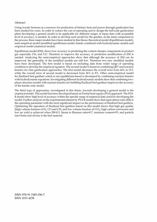
AbstractUsing woody biomass as a resource for production of biofuel, heat and power through gasification hasbeen studied for years. In order to reduce the cost of operating and to design the full-scale gasificationplant developing a general model to be applicable for different ranges of input data with acceptablelevel of accuracy, is needed. In order to develop such model for the gasifier, as the main component inthe process, three major models have been studied in this thesis; theoretical model (Equilibrium model),semi-empirical model (modified equilibrium model, kinetic combined with hydrodynamic model) andempirical model (statistical model).

Equilibrium model (EM), shows low accuracy in predicting the content ofmajor components in productgas especially CH4 and CO. Therefore to improve the accuracy of prediction modification of EM isneeded. Analyzing the semi-empirical approaches show that although the accuracy of EM can beimproved, the generality of the modified models are still low. Therefore two new modified modelshave been developed. The first model is based on including data from wider range of operatingcondition to develop the empirical equation. The second model is based on combining QET and reactionkinetics for char gasification approaches. The first model decreases the overall error from 44% to 31%while the overall error of second model is decreased from 36% to 8%. Other semi-empirical modelfor fluidized bed gasifiers which is not equilibrium-based is developed by combining reaction kineticswith hydrodynamic equations. Investigating different hydrodynamic models show that combining two-phase-structure model with reaction kinetics for bubbling fluidized bed gasifiers improves the accuracyof the kinetic-only model.

The third type of approaches, investigated in this thesis, towards developing a general model is theempirical model. This model has been developed based on Partial least square (PLS) approach. The PLS-R model show high level of accuracy within the specific range of empirical data used for developing themodel. Further analysis on the experimental dataset by PLS-R model show that equivalence ratio (ER) isthe operating parameter with the most significant impact on the performance of fluidized bed gasifiers.Optimizing the operation of fluidized bed gasifiers based on this model shows that high gas quality(high volume fraction of H2, CO and CH4 and low volume fraction of CO2), high carbon conversion andlow tar yield is achieved when ER≈0.3, Steam to Biomass ratio≈0.7, moisture content≈9% and particlesize≈3mm and olivine is the bed material.

ISBN 978-91-7485-296-7 ISSN 1651-4238

To my mother and father, that love me unconditionally

Acknowledgements

We’re alive of not keeping tranquility We’re waves, our rest is our vanity

ما زنده هب آنیم هک آرام نگیریم موجیم هک آسودگی ما عدم ماست

(Saaeb-e-Tabrizi) (صائب تبرزیی)

This thesis is based on a project started by Swedish Gasification Center, there-fore I would like to first acknowledge them for giving me this opportunity to taste the joy of research toward a brighter future. The way was long and not quite smooth, but finally the end was reached. This would probably not have happened had my guides not been there on the way. Therefore I would like to acknowledge all of them accordingly.

A wise person once said “never give up on your dreams” and so I didn’t. I would like to thank my main supervisor dear prof. Erik Dahlquist for trusting me on this project and never doubting my capabilities. I would also like to express my gratitude to Dr. Eva Thorin for always being there and supporting me both mentally and technically all the way. Similarly, I want to thank dear Dr. Hailong Li with whom I had the toughest but also the most fruitful discus-sions, and who taught me how to think scientifically and precisely!

I also gratefully thank dear prof. Alberto Gomez Barea for showing me the joy of being passionate about what I am doing. Further, I would like to sin-cerely thank my co-author and friend Jan Skvaril for being a supportive and hardworking team-mate. I would love to also express my gratitude to Dr. Raza Naqvi, Dr. Wennan Zhang for reviewing my thesis and Mikael Gustafsson for helping a lot with formatting and layout of this work.

I would love to thank my dear friends Zahra Mohammadi, Worrada Nookuea, Anbarasan Anbalagan, Lokman Hossein, Nima Ghaviha, Pietro Campana and colleagues in the department for all the conversations, cheering up and excitement that they brought to my PhD study time. I also want to express my gratitude to my best friends from Stockholm and Uppsala, Azadeh Hassannejad, Ehsan Roozbahani, Hamed Rafi and Zahra Khadji for their men-tal support and encouragement.

Last but not least I want to express all my love and gratitude to my family. My dear mother Katayoon Nikbakhsh, my lovely father Mohammad Javad Mirmoshtaghi and my supportive brother Peyvand Mirmoshtaghi - without you these years of hard work would have been so tough. Special thanks from the bottom of my heart go to my lovely nephew Mehrad Mirmoshtaghi who brought all the joy, motivation for life and happiness one needs to go through life’s ups and downs.

Summary

The use of wood biomass as a resource for biofuels, heat and electricity pro-duction through gasification has been studied for many years. Developing full-scale gasification plants and reducing operation costs require a general model in order to assess the impact of different operating conditions on the process. The general model should not only be applicable to different operating ranges, but should also provide acceptable accuracy. A major challenge in modeling of gasification is to model the gasifier, which is a main component of the pro-cess, in a sufficiently general way that can be used in system-level analysis. Three main approaches have been studied in this thesis; theoretical model (equilibrium model), semi-empirical model (modified equilibrium model, ki-netic combined with hydrodynamic model) and empirical model (statistical model).

The equilibrium model (EM) is used to investigate the thermodynamic lim-its of the gasification process, but it shows low accuracy for fluidized bed gasifiers (FB). The EM modification approaches are studied in this thesis by using: 1. Quasi-equilibrium temperature (QET); 2. Empirical correlations for light hydrocarbons conversion; and 3. Reaction kinetics for char gasification. Analysis of these approaches shows that accuracy of the EM can be improved, but the generality of the models is still low. Therefore, two new models have been developed. The first model is based on including data from a wider range of operating conditions to develop the empirical equation. The second model is based on combining QET and reaction kinetics for char gasification ap-proaches. The first model decreases the overall error from 44% to 31% while the second model decreases the overall error from 36% to 8%.

Additionally, other semi-empirical models for fluidized bed gasifiers have been investigated in order to study different phenomena occurring in the real case gasifier. These models are based on kinetic rate equations combined with different hydrodynamic modeling concepts; 1. Kinetic-only model (KIN); 2. Kinetic-only model combined with two phase structure model (TPT); and 3. Kinetic-only model combined with counter current back mixing (CCBM). Evaluation of these models with experimental data from different bubbling fluidized bed gasifiers shows that the TPT model provides the best agreement between prediction results and experimental data.

Finally, the empirical model approach is assessed on generality. An empir-ical model using the partial least square (PLS) approach is developed for a

large dataset of FBs. The results show that the model performs with high ac-curacy when the gasifiers are operated within the specific range of input pa-rameters used to develop the model. Multivariate analysis of the dataset shows that the equivalence ratio (ER) is the parameter with the most significant im-pact on the output. Optimizing the operation of FBs based on this model shows that high gas quality (high H2, CO and CH4 content and low CO2 content), high carbon conversion and low tar yield is achieved at ER≈ 0.3, S/B≈ 0.7, moisture content≈ 9% and particle size≈ 3mm with olivine as the bed material.

Sammanfattning

Att använda träbiomassa som en resurs för biobränslen, värme och elprodukt-ion genom förgasning har studerats under flera år. För att minska kostnaderna för drift och utveckling av fullskaliga förgasningsanläggningar och kunna be-döma effekterna av olika driftsförhållanden i processen behövs en generell modell. Den generella modellen bör inte bara kunna tillämpas inom olika driftsområden, utan den bör också ge en acceptabel noggrannhet. En stor ut-maning i modellering av förgasning är att modellera förgasaren, som är en av huvudkomponenterna i processen, på ett tillräckligt generellt sätt för att mo-dellen ska kunna användas i analys på systemnivå. Tre huvudsakliga tillväga-gångssätt har studerats i denna avhandling; teoretisk modell (jämviktsmodell), semi-empirisk modell (modifierad jämviktsmodell, kinetisk modell i kombi-nation med hydrodynamisk modell) och empirisk modell (statistisk modell).

En jämviktsmodell (EM) har använts för att undersöka de termodynamiska gränserna för förgasningsprocessen, men den visar låg noggrannhet för fluidi-serad bädd förgasare (FB). Till följd av detta har metoder för att modifiera EM studerats i denna avhandling genom att använda: 1.quasi-jämviktstemperatur (QET), 2. empiriska korrelationer för konvertering av lätta kolväten och 3. reaktionskinetik för kolförgasning. Analyser av dessa metoder visar att nog-grannheten i EM kan förbättras, men det är fortfarande utmanande att kunna få en modell som fungerar generellt. Därför har två nya modeller utvecklats. Den första modellen baseras på att data från ett bredare spektrum av driftstill-stånd används för att utveckla den empiriska ekvationen. Den andra modellen bygger på att kombinera QET och reaktionskinetik för kolförgasning. Den första modellen minskar det totala felet från 44% till 31%, medan det totala felet minskar från 36% till 8% när den andra modellen används.

För att öka kunskapen om olika fenomen som förekommer i verkliga för-gasare, har andra semi-empiriska modeller för fluidiseradbädd-förgasare un-dersökts i denna avhandling. Modellerna som har studerats baseras på kine-tiska hastighetsekvationer i kombination med olika hydrodynamiska modell-leringskoncept. Tre olika modeller har studerats i denna avhandling; 1. modell baserad på endast kinetik (KIN), 2. kinetisk- modell i kombination med två-fasstrukturmodell (TPT) och 3. kinetisk modell i kombination med motströms återblandning (CCBM). Utvärdering av noggrannheten av dessa modeller med hjälp av experimentella data från olika bubblande fluidiseradbäddförgasare visar att då TPT modell används får man bättre överensstämmelse mellan si-mulerade data och experimentella data.

Slutligen bedöms möjligheten att använda en empirisk modell för att uppnå generalitet. En empirisk modell har utvecklats i denna avhandling med partial least square (PLS) metoden för en stor mängd data från fluidiseradbäddförga-sare. PLS-R-modellen visar hög noggrannhet för FB förgasare så länge driften är inom det specifika område för vilken modellen har utvecklats. Baserat på multivariabel analys av datamängden är ekvivalensförhållandet (ER) den pa-rametermed som har den mest betydande inverkan på resultatet. Optimering av driften av FB baserat på denna modell, visar att hög gas kvalitet (hög halt av H2, CO och CH4 och låg halt av CO2), hög omvandling av kol och låg tjär-halt uppnås vid ER≈ 0.3, S / B≈ 0.7, fuktinnehåll≈ 9% och partikelstorlek≈ 3mm när olivin är bäddmaterialet.

List of papers

I. Mirmoshtaghi G, Li H, Dahlquist E, Thorin E. Bio-methane production through different biomass gasifiers. ICAE 2013. 2013. Pretoria. South Af-rica

II. Dahlquist E, Mirmoshtaghi G, Engvall K, Thorin E, Larsson E, Yan J. Modeling and simulation of biomass conversion processes. EU-ROSIM2013. 2013. Cardiff. UK.

III. Mirmoshtaghi G, Li H, Thorin E, Dahlquist E. Evaluation of different bi-omass gasification modeling approaches for fluidized bed gasifiers. Bio-mass and Bioenergy. 2016; 91, 69-82.

IV. Mirmoshtaghi G, Li H, Thorin E, Dahlquist E. Assessment on the impact of including hydrodynamics on the performance of kinetic based models for bubbling fluidized bed gasifiers. Submitted to Energy conversion and management.

V. Mirmoshtaghi G, Skvaril J, Campana PE, Li H, Thorin E, Dahlquist E. The influence of different parameters on biomass gasification in circulat-ing fluidized bed gasifiers. Energy conversion and management. 2016; 126, 110-23.

Not included Mirmoshtaghi G, Westermark M, Mohseni F. Simulation of a lab-scale

methanation reactor. ICAE 2012. 2012. Suzhou. China Song H, Guziana B, Mirmoshtaghi G, Thorin E,Yan J. Waste-to-energy

scenarios analysis based on energy supply and demand in Sweden. ICAE 2012. 2012. Suzho. China

Author’s contribution to the papers

The author did the modeling, experimental data collection, analysis of the re-sults and the majority of the writing in papers I, III and IV. The author per-formed the calculations and wrote the section regarding “equilibrium model-ing by Aspen Plus” in paper II, while most of the paper was written by the first author (Erik Dahlquist). Additionally, the author was responsible for the main idea, experimental data collection, final evaluation and most of the writ-ing of paper V.

Table of Contents

1 INTRODUCTION ...................................................................................... 1 1.1 Background ....................................................................................... 1 1.2 Scopes and research questions .......................................................... 3 1.3 Thesis outline .................................................................................... 5

2 LITERATURE REVIEW ............................................................................. 6 2.1 Different types of gasifiers ................................................................ 6 2.2 Gasification mechanism in fluidized bed gasifiers ........................... 8 2.3 Modeling biomass gasification-state of art ....................................... 9

3 METHODOLOGY ................................................................................... 16 3.1 Definition of parameters and indexes ............................................. 16 3.2 Equilibrium model and modification methods ................................ 17 3.3 Kinetics combined with hydrodynamics ......................................... 19 3.4 Principal component analysis (PCA), Partial least square (PLS) and Genetic algorithms (GA) .......................................................................... 23 3.5 Model evaluation............................................................................. 25

4 RESULTS AND DISCUSSION .................................................................. 27 4.1 Collected experimental data from different types of gasifiers ........ 27 4.2 General model for biomass gasification for system-level analysis . 30

4.2.1 Theoretical model (Equilibrium model) ................................ 30 4.2.2 Semi-empirical model ............................................................ 32

4.2.2.1 Modified EMs ............................................................. 32 4.2.2.2 Kinetic-combined-hydrodynamic model .................... 38

4.2.3 Empirical model (Statistical model) ...................................... 41 4.3 The key operating parameters influencing the biomass gasification in fluidized beds ....................................................................................... 44

5 CONCLUSION ........................................................................................ 52

6 FUTURE WORK ..................................................................................... 54

REFERENCES ................................................................................................. 55

PAPERS .......................................................................................................... 67

List of figures

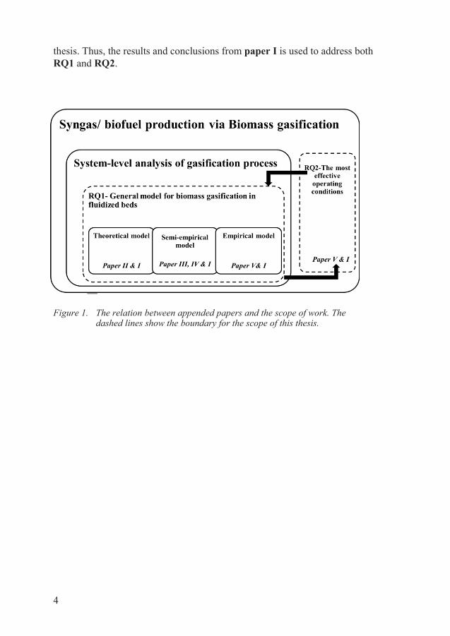
Figure 1. The relation between appended papers and the scope of work. The dashed lines show the boundary for the scope of this thesis. ................... 4

Figure 2. Changes in volume fraction of CH4 in dry product gas from different types of gasifiers at different ER values ................................................ 29

Figure 3. Changes in lower heating value (LHV) of the product gas from different types of gasifiers at different equivalence ratio (ER) values ................. 30

Figure 4. Comparison of equilibrium model and experimental results for the dry-nitrogen-free product gas composition from black liquor gasification (82) at different equivalence ratio (ER) values ...................................... 31

Figure 5. The recent comparison of equilibrium model and experimental results for the dry-nitrogen free product gas composition (a) H2, (b) CH4, (c) CO and (d) CO2 from black liquor gasification (82) at different equivalence ratio (ER) values including more data points ..................... 32

Figure 6. Average overall error level (OE) and variation for prediction of gas composition from bubbling fluidized bed (BFB) and circulating fluidized bed (CFB) gasifiers ................................................................. 33

Figure 7. Average overall error level (OE) and variation width (VW) in prediction of gas composition when (a) equivalence ratio (ER) value is fixed, (b) load is fixed, (c) temperature is fixed and (d) steam to biomass(S/B) ratio is fixed. In each case, other parameters than the fixed one are varying. The values for OE are shown by the columns and correspond to the left axis while VW is shown by lines matching the right axis. ........ 34

Figure 8. MOD-MODEL III flow sheet in Aspen plus ......................................... 38

Figure 9. Overview on development of kinetic-hydrodynamic models in this thesis ............................................................................................................... 39

Figure 10. Loadings plots which show the correlation existing between different parameters. The arrows indicate input and output parameters with negative correlation, while the small dashed circles indicate input and output parameters with positive correlation. .......................................... 45

List of tables

Table 1. Different types of gasifiers (16–18) .............................................. 7

Table 2. Major gasification reactions (4, 5) ................................................. 9

Table 3. Kinetics of heterogeneous and homogeneous gasification reactions....................................................................................... 21

Table 4. Equations used in different hydrodynamic sub-models in this study ............................................................................................ 22

Table 5. Experimental data different gasifiers investigated in this thesis . 28

Table 6. Overview of modified EMs for biomass gasification in fluidized bed gasifiers. The italic and bold text indicates the limitations that have been focused in further modifications . ...................... 37

Table 7. Average relative error (rel E) and average overall error (OE) of different models in predicting gas composition, gas yield and tar yield compared to the experimental data from BFB 4 (30), BFB 8 (23), BFB 1 (6) and BFB 7(85). .................................................. 40

Table 8. Complexity index for different kinetic based models in this thesis ..................................................................................................... 40

Table 9. Regression coefficients forming the PLS model for each component in the product gas, heating value, carbon conversion, dry gas yield and tar yield based on equation 3. .......................... 42

Table 10. Data points used for validation of the PLS model ....................... 43

Table 11. R2, RMSEP and average error (Ave E) for validation of the PLS model based on data in table 9 .................................................... 43

Table 12. P-values derived from regression coefficients of the PLS model in table 9. Colors are explained below. ........................................... 48

Table 13. Selected and representative results of optimization .................... 50

Nomenclature

Symbols

𝑨𝑨𝒃𝒃𝒃𝒃𝒃𝒃 Area of the bed m2 𝒃𝒃𝒏𝒏 The regression coefficient of n sample - 𝑪𝑪𝒊𝒊 Concentration of the component i kmol/m3 𝑪𝑪𝒂𝒂𝒂𝒂,𝒄𝒄 Concentration of the char in ascending phase kmol/m3 𝑪𝑪𝒃𝒃𝒂𝒂,𝒄𝒄 Concentration of the char in descending phase kmol/m3 𝑪𝑪𝑨𝑨𝒃𝒃 Concentration of component A in bubble phase kmol/m3 𝑪𝑪𝑨𝑨𝒃𝒃 Concentration of component A in emulsion phase kmol/m3 𝑪𝑪𝒖𝒖𝒖𝒖𝒖𝒖𝒊𝒊 Biomass carbon content based on ultimate analysis %-dry based 𝑫𝑫𝑨𝑨𝑨𝑨 Gas diffusion coefficient m2/s 𝒃𝒃𝒑𝒑𝑪𝑪𝑪𝑪𝒂𝒂𝑪𝑪 Char particle size m 𝒃𝒃𝒃𝒃 Bubble diameter m 𝒃𝒃𝒃𝒃𝒃𝒃 Maximum bubble diameter m 𝒃𝒃𝒃𝒃𝟎𝟎 Minimum bubble diameter in the entrance m 𝒃𝒃𝑭𝑭𝑪𝑪𝒃𝒃 Diameter of freeboard section m 𝒃𝒃𝒃𝒃𝒃𝒃𝒃𝒃 Diameter of bed section m 𝒇𝒇𝒂𝒂𝒂𝒂 Fraction of ascending phase in the bed m3 asc. phase/m3 bed 𝒇𝒇𝒃𝒃𝒂𝒂 Fraction of descending phase in the bed m3 desc. phase/m3 bed 𝑮𝑮𝒚𝒚 Gas yield m3 produced gas/kg biomass 𝑪𝑪𝒃𝒃𝒃𝒃𝒃𝒃 Bed height m 𝑪𝑪𝑭𝑭𝑪𝑪𝒃𝒃 Freeboard height m 𝑯𝑯𝒖𝒖𝒖𝒖𝒖𝒖𝒊𝒊 Biomass hydrogen content based on ultimate analysis

(dry based) %

𝑲𝑲𝒃𝒃𝒄𝒄 Transfer coefficient bubble to cloud 1/s 𝑲𝑲𝒃𝒃𝒃𝒃 Transfer coefficient bubble to emuslion 1/s 𝑲𝑲𝒄𝒄𝒃𝒃 Transfer coefficient bubble to cloud 1/s 𝑲𝑲𝒘𝒘 Wake exchange coefficient 1/s 𝑲𝑲𝑬𝑬𝑬𝑬 Equilibrium constant of water gas shift reaction - Load Cross sectional flow of the biomass kg/m2.h or Mg/m2.h 𝑴𝑴𝒊𝒊 Molar flow rate of component i kmol/s 𝑴𝑴𝑴𝑴𝒊𝒊 Molar weight of component i g/mol 𝒏𝒏𝒐𝒐𝑪𝑪𝒇𝒇 Number of orifice openings 𝑶𝑶𝑬𝑬𝒊𝒊 Overall error in predicting each i component - 𝑶𝑶𝒖𝒖𝒖𝒖𝒖𝒖𝒊𝒊 Biomass oxygen content based on ultimate analysis %-dry based 𝑷𝑷𝒊𝒊 Partial pressure of component i atm 𝑪𝑪𝑨𝑨𝒃𝒃 Reaction rate for component A in bubble phase kmol/m3.s 𝑪𝑪𝒊𝒊 Reaction rate for component i kmol/m3.s 𝑪𝑪𝒃𝒃𝒖𝒖𝑬𝑬𝒊𝒊 Relative error in predicting component i - 𝑻𝑻 Temperature °C 𝑻𝑻𝒃𝒃𝒃𝒃𝒃𝒃 Bed temperature K 𝑻𝑻𝑭𝑭𝑪𝑪𝒃𝒃 Freeboard temperature K

𝒖𝒖 Superficial gas velocity m/s 𝒖𝒖𝒂𝒂𝒂𝒂 Ascending phase velocity m/s 𝒖𝒖𝒃𝒃 Bubble phase velocity m/s 𝒖𝒖𝒃𝒃𝒃𝒃 Bubble rise velocity m/s 𝒖𝒖𝒅𝒅𝒂𝒂 Descending phase velocity m/s 𝒖𝒖𝒆𝒆 Emulsion phase velocity m/s 𝒖𝒖𝒎𝒎𝒎𝒎 Minimum fluidization velocity m/s 𝑿𝑿 Input variables - 𝑿𝑿𝒄𝒄𝒄𝒄𝒄𝒄𝒄𝒄 Instantaneous char conversion - 𝒀𝒀 Variable to be predicted as output Dependent on the case 𝒚𝒚𝒊𝒊𝒆𝒆 Experimental results for component i Dependent on the case 𝒚𝒚𝒊𝒊𝒊𝒊 Predicted results for component i Dependent on the case ��𝒚 Average value of experimental results for component i Dependent on the case 𝒛𝒛 Reactor height m

Greek symbols

𝜹𝜹 Bubble fraction in fluidized bed m3 bubble/m3 bed 𝜺𝜺𝒎𝒎𝒎𝒎 Voidage at minimum fluidization velocity m3 void/m3 bed 𝜺𝜺𝒆𝒆 Voidage in emulsion phase m3 void/m3 emulsion 𝜺𝜺𝒃𝒃 Voidage in bubble phase m3 void/m3 bubble 𝝁𝝁 viscosity Pa.s 𝝆𝝆𝒈𝒈 Gas density kg/m3 𝝆𝝆𝒂𝒂 Solid density kg/m3

Abbreviations

𝑨𝑨𝒄𝒄𝒆𝒆. 𝑬𝑬 Average error - BFB Bubbling fluidized bed CFB Circulating fluidized bed CNG Clean natural gas DME Dimethyl ether ECN Energy Research Centre of the Netherlands EM Equilibrium model ER Equivalence ratio FBG Fluidized bed gasifiers FC Fixed carbon FW Foster Wheeler GA Genetic algorithm HHV Higher heating value MJ/m3 ID Internal diameter m IEA International energy agency KTH Kungliga Tekniska Högskolan LHV Lower heating value MJ/m3 LNG Liquid natural gas LNU Linneuniversitet MC Moisture content MDH Mälardalen Högskola OE Average overall error PC Principal component PCA Principal component analysis PLS Partial least square

QET Quasi-equilibrium temperature 𝑹𝑹𝟐𝟐 R-square - RCSTR Continuous stirred tank reactor in Aspen plus rel Ei Average relative error for each component Rel Eij Relative error for each component at each set point RGIBBS Gibbs reactor in Aspen plus 𝑹𝑹𝑹𝑹𝑹𝑹𝑹𝑹𝑹𝑹 Root mean square of prediction RQ Research question RSTOIC Stoichiometric reactor in Aspen plus RYIELD Yield reactor in Aspen plus 𝑹𝑹𝑩𝑩

Steam to biomass ratio -

𝑽𝑽𝑽𝑽 Variation width WGS Water gas shift reaction

1

1 Introduction

1.1 Background Environmental concerns such as global warming and climate change are driv-ing countries to invest in science and infrastructure to extract energy from re-newable resources as a substitute for fossil fuel resources. In addition, coun-tries with limited or no fossil fuel resources, such as Sweden, are economically motivated to transition to renewable and sustainable resources.

The International Energy Agency (IEA) presented a Sankey diagram which showed that the transportation sector has one of the largest shares of world energy use (around 30%). Therefore managing the energy use in this sector will play a crucial role in the path towards a more sustainable society (1). Based on the most recent data presented by IEA, the current share of biofuel and waste used for the transportation sector worldwide is small (less than 3%), so research and development projects focusing on alternative fuels and re-sources are essential to increase sustainability.

Due to the safety and environmental concerns with conventional vehicle fuels such as gasoline and diesel, natural gas in the form of compressed natural gas (CNG) and liquefied natural gas (LNG) has been considered as a more “clean” alternative among fossil fuels. However, natural gas is still classified as a non-renewable and unsustainable fossil fuel. Bio-methane is a renewable substitute for natural gas which is the methane produced from bio-based ma-terial. It generates more heat per unit mass and fewer toxic and hazardous emissions compared to other hydrocarbons and fossil fuels (2). Moreover, it can be distributed and used by the existing infrastructure, whereas other re-newable fuels such as hydrogen require changes in distribution and engine design. Compared to available renewable fuels such as ethanol, DME and methanol, bio-methane production requires fewer synthetic unit operations which makes it a less complex process (3).

Among the different paths for biomass to energy, gasification is one of the most general and promising thermochemical technologies to convert any car-bonaceous fuel to gas with considerable heating value (4). Gasification begins by rapid devolatilization of the solid fuel, in which volatiles are separated from the solid fuel, leaving char. Next, volatile combustion followed by homoge-neous reactions between volatile components occur. These reactions are exo-thermic while char gasification is endothermic overall. Some of the fuel can be combusted to provide the heat demand of the endothermic reactions and thus the system can operate autothermally (5). Depending on the type and de-sign of the gasifier these steps can occur stage-wise or simultaneously.

Gasification of biomass with different objectives such as biofuel, heat and power production have been studied for several decades. For instance, during

2

the 1970s and the early 1980s, there have been gasification plants in Sweden (Termiska processer AB (TPS) plant), at Texas Technological College and Texas A&M University (6). In 1998, the first successful circulating fluidized bed (CFB) gasifier plant was built by Foster Wheeler Energia Oy in Lahti, Finland to produce power and heat. This gasifier has been in commercial op-eration since then. Subsequently, AE/Repotec started building a dual bed gas-ifier at Güssing, Austria in 2000, which began commercial operation in 2001. This plant was designed for combined heat and power (CHP) production. In 2002, ECN (Energy Research Centre of the Netherlands) constructed the MILENA gasifier, which is based on the concept of indirect biomass gasifica-tion. Other operation units such as gas cleaning, methanation unit and further upgrading units have also been considered in connection to MILENA. During this time, synthetic natural gas (SNG) production from biomass became the main area of interest for researchers. For example, the Paul-Scherre institute (PSI) in Switzerland has studied dry biomass conversion to SNG over a ten-year period, while the center for solar energy and hydrogen research (ZSW) in Stuttgart, Germany has been focused on development of a technology called Absorption Enhanced gasification/Reforming (AER) . AER is a type of dual bed biomass gasification which results in a product gas with high hydrogen content (7).

In order to convert solid biomass to biofuel through gasification, solid ma-terial must be dried and chipped into a required size suitable for the process. Based on the specific design of the gasifier, solid particles are then fed to the gasifier either from the bottom or top. The raw syngas, which is produced via gasification, mainly consists of H2, CO, CO2 and around 2-15% CH4. After tar removal, the gas passes through a water-gas shift reactor to adjust the C/H ratio so that it is suitable for the methanation reaction or for production of other biofuels such as methanol or DME. The most conventional methanation reactor is a Ni-based catalytic reaction in which CO and H2 are converted to CH4 and H2O. However there have been studies (8,9) in which a Sabatier re-action1 on Ru-based catalyst is also considered for methane production.

Evaluation of the biofuel or power production via gasification of the bio-mass at the industrial scale requires system-level analysis. System-level anal-ysis involves consideration of factors such as including and excluding differ-ent unit operations to increase the thermal/electrical efficiency of the system, and integration of different parallel processes to reduce CO2 emission or en-ergy use in the process. Since the most important unit in the process is gasifier, a model is needed for this unit that functions accurately with limited data on the scale, dimension and detailed design. This model should be able to predict gas composition with an acceptable degree of accuracy for different ranges of

1. The exothermic catalytic reaction converts H2 and CO2 to water and CH4. It is named after the Belgian chemist who first investigated the role of nickel catalyst on hydrogenation and hy-drocarbons in 1902.

3

operating conditions. Several different efforts have been made to model gasi-fiers (10–13), most of which were developed for designing gasifiers with spe-cific geometry and size. However there has been little focus on the generality aspect of the models for system-level analysis. The main focus of this thesis is to develop a general model for the complex thermochemical system of gas-ification.

1.2 Scopes and research questions Based on the necessary steps for system-level design of the process and to address the main focus of this thesis, developing a general model for gasifica-tion, the following research questions are proposed:

RQ1. How to develop a general and accurate model for biomass gasification to be used in system-level analysis?

RQ2. What are the operating parameters with the most significant impact on the product gas composition of biomass gasification?

This thesis is divided in two main parts, the first part is based on model devel-opment, validation and evaluation to address RQ1 while the second part is based on the evaluation of the experimental data collected from the literature using the models from the first part to address RQ2. It is important to mention that prior to any attempt for addressing RQ1 and RQ2, experimental data are collected from different types of gasifiers which are reported in a separate section. The connection between different RQs, research field and appended papers are shown in figure 1. The dashed-line boundaries highlighting the RQs while the solid-line boundaries show the area in the research field. As the fig-ure shows, the knowledge and data derived from the first part will also be used to address RQ2 while the knowledge from second part will be used as input data to address RQ1.

In order to address RQ1, three different approaches of modeling fluidized bed gasifier have been studied in papers II, III, IV and partially in paper V. Paper II mainly evaluates the equilibrium model, which is a theoretical model. Papers III and IV examine semi-empirical approaches based partly on fundamental theory and partly on empirical correlations. Paper V assesses empirical approaches to modeling fluidized bed gasifiers. The results from this paper are also used to determine the operating parameters with the most sig-nificant impact on the gasifiers’ performance and gas quality to address RQ2. Paper I studies the impact of gasifier type as one of the influencing operating parameters on quality of the product gas while also providing the experimental data required for development, validation and evaluation of the models in this

4

thesis. Thus, the results and conclusions from paper I is used to address both RQ1 and RQ2.

• Syngas / bio fuel pro ductio n via Bio mass gas ification •

Figure 1. The relation between appended papers and the scope of work. The dashed lines show the boundary for the scope of this thesis.

5

1.3 Thesis outline The thesis is divided into 6 main chapters as following:

Chapter 1. Introduction This chapter presents the background, scope, research questions and thesis outline to prepare the reader for subsequent chapters and highlight the discus-sions and results.

Chapter 2. Literature review The literature review is designed to acknowledge previous studies in the field and outline the current knowledge gap. This provides the knowledge base to understand the need for this research.

Chapter 3. Methodology The methodology and tools used to address the given RQs in this thesis are presented and explained. The major part of the methodology is dedicated to different modeling approaches while the methods for data collection and anal-ysis in each paper are also presented.

Chapter 4. Results and discussion This chapter contains the results and discussion related to the analysis of ex-perimental data and different approaches towards developing a general and accurate model for simulation of biomass gasification, especially in fluidized bed gasifiers.

Chapter 5. Conclusion The conclusions of this thesis are presented based on the RQs presented in Chapter 1.

Chapter 6. Future work Future work for the continuation of this research is listed and explained.

6

2 Literature review

2.1 Different types of gasifiers A gasifier generally consists of one or two vessels filled with solid particles as bed material, with the exception of entrained flow gasifiers. Depending on the designed heating system, gasifiers can be operated either autothermally (adiabatic) or allothermally (isothermal). Table 1 presents different types and designs of gasifiers, with an example of a pilot/demonstration for each specific design. These gasifiers differ in the range of major operating parameters, physical structure and consequently the product gas composition. For in-stance, as explained by Knoef (14) , the product gas from entrained-flow gas-ifiers has a very low methane and tar content, while the syngas from updraft fixed bed and fluidized bed gasifiers (FBG) has relatively higher methane and tar content. Updraft fixed bed gasifiers produce a gas with high tar content and a large amount of pyrolysis products, which requires extensive gas cleaning before further use in the gas/power grid. Conversely, downdraft fixed bed gas-ifiers produce cleaner gas while it cannot be used for large capacity power production due to the upscaling limitations of fixed bed gasifiers (14). In the case of FBGs, fluidization provides a uniform temperature distribution which helps to increase carbon conversion efficiency and production of gas with high heating value. However, drawbacks of FBGs include tar formation and the necessity for temperature control to prevent agglomeration in the bed. FBGs are easy to scale up and operate with feedstock of different types and sizes (15).

7

Table 1. Different types of gasifiers (16–18)

Gasifier type Gasifier specific design

Temp. & press. range

Description Example of pi-lot/demonstration rig

Fixed bed/ Moving bed

Updraft 300–1,000°C atm.

Fuel is fed from the top and gasification agent flows from the bottom of the reactor. The process steps are drying, pyroly-sis, reduction and oxida-tion respectively.

Ansager plant: 200 kW pilot plant integrated with Stirling en-gine in 2006

Downdraft 300–1,000°C atm.

Fuel is fed from the top of the reactor. The gasifi-cation agent is fed into the middle of the reactor. Syngas is extracted from the bottom. The process steps are drying, pyroly-sis, oxidation and reduc-tion.

Xylowatt sa gasi-fier integrated with CHP in Ga-zel in Belgium The size is 0.15 MWe output.

Fluidized bed

Bubbling flu-idized bed

(BFB)

650–950°C 1–35 bar

Fuel is fed above the sand bed and the gasification agent enters the reactor from the bottom. The syngas is extracted from the top after being cleaned in cyclones.

Foster Wheeler (FW) Eco gas gasifier in Finland for syngas pro-duction to be combusted in steam boiler with 40 MWth output size.

Circulating fluidized bed

(CFB)

800–1,000°C 1–19 bar

Fuel is fed to the sand bed while the gasification agent enters the reactor from the bottom. Syngas is partly extracted from the top and partly recy-cled to the bottom of the gasifier again. The fluidi-zation velocity is higher than in BFB.

FW Lahti in Fin-land with 40–70 MWth input ca-pacity connected to a CHP unit.

Entrained flow

Entrained flow-down

flow

> 1,200°C > 20–50 bar

Powder or slurry fuel is mixed with the gasifica-tion agent and enters to the reactor from the top. The gasification is aided by a powderized flame. Syngas is extracted from the bottom.

3–5 MWth Bioliq gasifier operates in Germany to synthesize biofuel from syngas

Entrained flow-up flow

1,050–1,400°C 27.5 bar

Feed and gasification agent enters from the bot-tom, so the gas flow is upward. The rest of the process is similar to the down flow gasifier.

No plant for bio-mass gasification is found.

8

Based on the information given in table 1, it is necessary to consider the im-pact of gasifier type as one of the influencing parameters to produce high qual-ity gas through gasification. Evaluating different types of gasifiers and com-paring the product gas quality in each available case would provide a better overview of the impact of this parameter on the quality of the product gas and overall performance of the system.

Considering fluidized bed gasifiers as a potential alternative for high qual-ity syngas and bio-methane production, the specific differences in design and operation of these gasifiers affect the gasification mechanism. For instance, in CFBs, solid particles in the product gas circulate to the bottom of the reactor. This supplies the heat demand for the endothermic reactions and also de-creases the tar formation rate by combusting the unreacted carbon. Carbon conversion efficiency is higher in CFB compared to bubbling fluidized beds (BFB) due to the better mixing, longer residence time for carbon particles and better solid-gas contact in high fluidization velocity (19). CFB can also oper-ate on biomass with a wider range of particle size and shape compared to BFB. However, BFB is more developed than CFB and has been more studied since it is simpler and easier to build and operate (14). Knowing the gasification mechanism in fluidized bed gasifiers provides the knowledge base needed for biomass to biofuel process design via gasification in this type of gasifiers.

2.2 Gasification mechanism in fluidized bed gasifiers The gasification process consists of different interrelated steps and reactions. A component can simultaneously play the role of reactant and product when multiple reactions occur. Therefore to deal with such a complex chemical sys-tem, further analysis and investigation is required on the impact of each oper-ating parameter on the quality of the product gas (4). Increasing knowledge regarding how the gasification reactions occur in fluidized bed gasifiers helps to improve analysis of different operating parameters impact on the quality of the product gas. The most characterized gasification reactions are listed in ta-ble 2 alongside the heat of reaction at the reference temperature of 298 K. The reactions are collected from the study by Higman and Van der Burgt (4) and Gomez Barea, Leckner (6).

9

Table 2. Major gasification reactions (4, 5)

Category of reactions

Reactions Heat of reac-tion at refer-

ence tempera-ture of 298 K ∆H (kJ/mol)

Name of reactions

Char combustion 𝐶𝐶 + 𝑂𝑂2 ⟶ 𝐶𝐶𝑂𝑂2

-394 Complete combus-tion

𝐶𝐶 + 0.5𝑂𝑂2 ⟶ 𝐶𝐶𝑂𝑂 -111 Partial combustion Char gasification

𝐶𝐶 + 2𝐻𝐻2 → 𝐶𝐶𝐻𝐻4 -75 Methanation

𝐶𝐶 + 𝐶𝐶𝑂𝑂2 → 2𝐶𝐶𝑂𝑂 +173 Boudouard

𝐶𝐶 + 𝐻𝐻2𝑂𝑂 → 𝐶𝐶𝑂𝑂 + 𝐻𝐻2 +131 Steam gasification

Homo- geneous volatile reactions

𝐶𝐶𝐻𝐻4 + 𝐻𝐻2𝑂𝑂 → 𝐶𝐶𝑂𝑂 + 3 𝐻𝐻2 +206 Methane Reforming

𝐶𝐶𝑂𝑂 + 𝐻𝐻2𝑂𝑂 ⇌ 𝐶𝐶𝑂𝑂2 + 𝐻𝐻2 -41 Water gas shift

𝐶𝐶𝑂𝑂 + 0.5𝑂𝑂2 → 𝐶𝐶𝑂𝑂2 -283 Carbon monoxide oxidation

𝐶𝐶𝐻𝐻4 + 2𝑂𝑂2 → 𝐶𝐶𝑂𝑂2 + 2𝐻𝐻2𝑂𝑂 -283 Methane oxidation

𝐻𝐻2 + 0.5𝑂𝑂2 → 𝐻𝐻2𝑂𝑂 -242 Hydrogen oxidation

Tar reactions 𝐶𝐶𝑛𝑛𝐻𝐻𝑚𝑚 + 𝑛𝑛 𝐻𝐻2𝑂𝑂 → 𝑛𝑛 𝐶𝐶𝑂𝑂 + (𝑚𝑚

2 + 𝑛𝑛) 𝐻𝐻2 Highly endo-

thermic (+200 to 300)

Steam reforming

𝐶𝐶𝑛𝑛𝐻𝐻𝑚𝑚 + (𝑛𝑛2)𝑂𝑂2 → 𝑛𝑛 𝐶𝐶𝑂𝑂 + (𝑚𝑚

2 ) 𝐻𝐻2 Partial oxidation

𝐶𝐶𝑛𝑛𝐻𝐻𝑚𝑚 + 𝑛𝑛 𝐶𝐶𝑂𝑂2 → 2𝑛𝑛 𝐶𝐶𝑂𝑂2 + (𝑚𝑚2 ) 𝐻𝐻2

Dry reforming

𝐶𝐶𝑛𝑛𝐻𝐻𝑚𝑚 + (2𝑛𝑛 − 𝑚𝑚2 )𝐻𝐻2 → 𝑛𝑛 𝐶𝐶𝐻𝐻4

Hydrogenation

𝐶𝐶𝑛𝑛𝐻𝐻𝑚𝑚 → (𝑚𝑚4 ) 𝐶𝐶𝐻𝐻4 + (𝑛𝑛 − 𝑚𝑚

4 ) 𝐶𝐶 Thermal cracking

2.3 Modeling biomass gasification-state of art According to a perspective paper written in 2011 by Upadhye et. al (20) on conceptual design of a new process, if an improvement/failure costs 1$ at the conceptual design stage, it will cost 100$ at the detailed design stage, 1000$ in the construction stage and 10,000 $ when the full implemented process fails. Therefore, it is economically beneficial to develop a design model to identify how the input parameters influence the final results before proceeding to de-tailed design and construction of a plant.

Biomass gasification in fluidized bed gasifiers is a fairly complex thermo-chemical process, which means that there are interrelations between operating

10

parameters and the way they impact the final product gas quality. Although there have been several studies analyzing gasification mechanisms, kinetics and hydrodynamics of the bed for system-level or component-level modeling (11,21–23), knowledge gaps on the interrelation between operating parame-ters and reactions still remain. In order to test the impacts of different param-eters on the quality of the product gas and determine the potentials for process integration, a general model for the gasifier should be developed to be used later in process design. The study by Yan et al (11) and Bilodeau et al (23) are at component level and focus on analyzing coal and biomass gasification mechanisms respectively in one specific BFB gasifier. In these studies, reac-tion kinetics and bed hydrodynamics are included in the model to predict the composition profile along the gasifier. Studies by Beheshti et al (21) and Ghassemi et al (22) focus on system-level modeling, however the generality of the model (providing high accuracy under different operating conditions) has not been assessed.

Identification of the most influential parameters on the raw syngas quality is one of the important outcomes of developing a general model. As explained above, general models are those that can be used for a wider range of operating parameters with limited data on the size, design and scale of the gasifier. Ali-muddin et. al (24) published a survey in 2010 based on listing the outcomes of different previous/ongoing efforts in lignocellulosic biomass gasification in fluidized beds qualitatively. These efforts are either performed on a limited and small variation of specific operating parameters (25,26) or designed only to test the impact of one specific novelty in the type of feedstock or bed ma-terial (27,28). Knowing the most influential parameters in a qualitative sense is useful, but a quantitative analysis of different fluidized bed gasification plants is needed to find the significance of each parameter on influencing the product gas quality. The typical parameters influencing the gas composition are bed material, bed temperature, gasification agent type and flow, and bio-mass type and size. Choosing a bed material with a catalytic effect would change the product gas composition. Bed material may be catalytically passive which makes it act solely as a surface to increase gas-solid contact, however using tar cracking catalysts as the bed material is considered as the primary tar removal step. Temperature is one of the operating parameters that influence the gas composition. High temperature reduces tar content in the gas while also decreasing the possibility of producing light hydrocarbons such as CH4. This parameter is controlled either by external cooling facilities or gasification agent flow. The auto-thermal characteristics of gasification reactions in FBGs suggest that gasifier temperature is controlled by gasification agent flow. The type of gasifying agent also influences the gasification reaction selectivity

11

(24). Different types of biomass would have different ultimate2 and proximate3 analyses, which clearly affect the composition of the product gas. The size of biomass particles also influence the possibility of contact between solid and gas, thus changing the reaction rates.

The main unit operation of the process, the gasifier, needs to be modeled with an acceptable level of accuracy. The required level of accuracy for mod-els is mainly determined by the final goal of the process and the intended ap-plication of the product gas. The product gas can be used as fuel or feedstock in different applications such as CHP plants, Fischer Tropsch (FT) synthesis plant, MeOH plant etc., with different gas quality requirements. According to the reviews by Gomez and Leckner (5) and Puig-Arnavat (29), and the study by Radmanesh (30), there are three major approaches for modeling gasifica-tion in fluidized beds: theoretical models such as the equilibrium model (EM), semi-empirical (EM-based models, kinetic combined with hydrodynamic models) and empirical models (statistical models). The equilibrium model (EM) is used for understanding and predicting the thermodynamic constraints for the operating parameters in the gasification process. The EM actually as-sumes that the final products achieve a stable composition in the chemical equilibrium state. The EM is based on thermodynamic analysis and does not require information on the dimensions, capacity and structure of the gasifier, which makes it suitable for concept studies and preliminary design of the pro-cess (31–33). The EM has been applied when all steps considered to be at equilibrium (32), or when only the pyrolysis step is at equilibrium (23,33). The EM is applicable mainly when the operating temperature is high and the residence time is longer than the time required for completion of all the gasi-fication reactions. However, the EM may not provide accurate results at low operating temperatures (750–900 °C) (5). The EM also has limitations when predicting light hydrocarbons and unconverted solid carbon content in the fi-nal product gas. There are two approaches for using the EM; 1. Stoichiometric; and 2. Non-stoichiometric. The stoichiometric equilibrium model is based on defined reactions, whereas in non-stoichiometric equilibrium models the spe-cific reactions are not known (5). Therefore non-stoichiometric equilibrium models are more suitable when detailed information about the reactions oc-curring in the chemical system is not available. Although the EM is suitable for developing a general model, the limited accuracy of the predictions by this model leads to “non-generality” factors. Therefore, a systematic study for evaluation of different available modification methods (34–38) and mapping the barriers and complexities leading to “non-generality” is essential for any further development of any general model.

2. Ultimate analysis shows the weight percent of C, H, O, S, N and ash in 1 unit of solid feed-stock. 3. Proximate analysis shows the weight percent of moisture, fixed carbon and volatile material in 1 unit of solid feedstock

12

There have been several studies to improve the accuracy of the EM in predict-ing product gas composition through different types of gasifiers. For instance, there are studies on gasification of coal by fluidized bed (39), gasification in entrained flow bed (10), biomass gasification in a downdraft gasifier (40) and fluidized bed gasifiers (32,41,42). The EM modification approaches can be categorized into three groups, all of which fall in the category of semi-empir-ical approaches:

1. Modifying the equilibrium temperature by the quasi-equilibrium temper-ature (QET) method. QET is a temperature different from the operating temperature, at which the selected chemical reaction is assumed to attain equilibrium (29,42). One way to determine the QET is to find the temper-ature at which the difference between the real content of components in the product gas and the values calculated by the EM is at a minimum. This was done by Doherty et al (43) to simulate biomass gasification in a CFB gasifier using the restricting equilibrium of the methane reforming reac-tion, CO-shift and ammonia formation reactions to different quasi-equi-librium temperatures.

2. Adding empirical correlations for the conversion of specific components to the existing equilibrium model. An example of this approach is the use of empirical correlations relating the content of carbon conversion, light hydrocarbons and ammonia in product gas to ER value as proposed by Hannula and Kurkela (44).

3. Introducing kinetics of major gasification reactions combined with bed hydrodynamics. This was done in the study by Nikoo and Mahinpay (45) by implementing the reaction kinetics of char combustion and gasification in an external subroutine using the Fortran language.

The study by Gomez and Leckner (5) partially discussed the generality of the EM for fluidized bed gasifiers. The criteria for this evaluation was based on the capability of different modified EMs to predict the composition of the product gas at different operating conditions. They concluded that the quasi-equilibrium approach gives the most accurate results for gas composition, but tar and char content cannot be predicted as generally as other components. In 2001, Kersten (42) reviewed and compared different EM modification ap-proaches for biomass gasification in fluidized bed gasifiers. He studied two approaches: 1. implementing empirical correlations as in the Schläpfer model (46); and 2. using the QET, as in the Gumz model (47). Kersten concluded that the QET model predicts gas composition more accurately in different op-erating conditions. Li et al (32,48) analyzed different methods for improving the accuracy of the EM in biomass air gasification in circulating fluidized beds (CFB). They found that adding empirical correlations for light hydrocarbons (mainly CH4) and carbon conversion improves the accuracy of the EM. Re-cently, Lim and Lee (41) developed a quasi-equilibrium model for fluidized

13

bed gasifiers. This model was based on 43 experimental datapoints from dif-ferent CFB (49,50) and BFB (51,52) gasifiers. They concluded that for better accuracy of quasi-equilibrium models, the empirical correlations should be adjusted to the experimental data collected from the same plant that is modeled by quasi-equilibrium model. Researchers such as Bilodeau et al (23), Nikoo et al (45) and Wang et al (12) have studied the possibility of improving the accuracy of the EM by considering reaction kinetics. In these studies, the py-rolysis step is assumed to be at equilibrium, whereas char gasification and some of the homogeneous reactions are considered to be kinetically con-trolled. The conclusion of these studies is that this method improves the accu-racy of the EM to an extent, but it also increases the complexity of the models, as explained by Gomez and Leckner (5).

In addition to studies on equilibrium-based models for gasification through fluidized bed gasifiers there are other types of semi-empirical approaches. Based on the categories described by Gomez and Leckner (5), fluidized mod-els (FM) (models formed by hydrodynamic equations) are mainly developed to provide better understanding of the physical-chemical interactions inside the gasifier. Composition and temperature profile are two additional expected outcomes of these models. Combination of reaction kinetics and different FMs for BFBs have been used for modeling fluidized bed gasifiers in different stud-ies by Yan et al (11), Beheshti et al (21), Bilodeau et al (23), Fiaschi et al (53), Radmanesh et al (30), Andersson and Karlsson (54), Asadi et al (55), and Ra-fati et al (56). There are also studies on gasification in downdraft gasifiers by Wang et al (12), Di Blasi et al (57) and Sharma et al (13) which can be con-sidered as equivalent to kinetic-only models for gasification in fluidized bed gasifiers. Among these studies, only Asadi et al (55) and Rafati et al (56) eval-uated the applicability of the model to different operating conditions. How-ever, the impacts of feeding point and different types of feedstock on the gas composition have not been analyzed. The studies mentioned here have not compared the performance of different types of hydrodynamic models, while in this thesis one of the assessments is on the performance of each fluidization model. It is important to mention that in the study by Fiaschi et al (53), only one type of hydrodynamic equations (simple two phase theory) was studied by comparing the overall accuracy of kinetic-only model and kinetic-com-bined-hydrodynamic model for one specific gasifier. In the thesis work by Andersson and Karlsson (54), there was a preliminary test of the idea of in-cluding different hydrodynamic models and assessing their impact on the ac-curacy and performance of kinetic-combined-hydrodynamic models. How-ever the models in that study have been completely changed in this thesis.

There are three major hydrodynamic models; two phase theory, counter current back mixing, and bubble assemblage (58–60). These models have been improved over the last few decades. These models are all based on the simple two phase theory (49) which divides the fluidized bed into bubble and emul-sion phases and assumes that the reactions occur only in the emulsion phase

14

and this phase is at minimum fluidization velocity (62). Following to the sim-ple two phase theory model, Mostoufi et al (63) have developed, a modified version of this model that is presented as two phase structure model. In this model, the reactions are assumed to occur in both emulsion and bubble phases and emulsion phase velocity varies by bubble phase velocity. In addition to two phase structure model, other efforts have been done to modify two phase theory model. One of the approaches is to consider the bubble diameter growth along the reactor height. This is the basis of the bubble assemblage hydrody-namic model (23,64). The other hydrodynamic model is counter current back mixing which includes the back mixing effect of the solid phase (char) in the bed which actually happens in the fast fluidization regime (58,65). Studying the accuracy and generality of different combination of these models and the kinetic-only model gives a better understanding towards developing an accu-rate model that can be applicable for different operating conditions.

Additionally, experience shows (44,66,67) that a simple empirical-statisti-cal-based model can provide the basis for predicting the effect of different operating conditions on the quality of product gas without considering any complex physical concepts. Therefore, the other model developed for biomass gasification in fluidized bed gasifiers in this thesis is an empirical model based on a multivariate statistical analysis approach. Due to the multivariate nature of this approach, the simultaneous variation of different operating parameters is considered when developing the empirical model. Thus, this model can pro-vide new knowledge on interactions between different operating parameters and their impact on the process performance. This can improve the available scientific knowledge for operating and controlling biomass gasification in flu-idized bed gasifiers. Multivariate analysis, specifically by principal compo-nent analysis (PCA) and partial least square (PLS) methods, is suitable for capturing the correlations in a complex system, like gasification, and for ana-lyzing the sensitivity of the system to the simultaneous variation of different parameters (68,69).

Using a large dataset with wide variation of input data to develop the em-pirical model would improve the generality of the model. In addition, using multivariate statistical approaches (such as PCA and PLS in this thesis) makes the observed correlations more reliable than univariate and bivariate analysis (70,71). For instance, including different types of feedstock and the variation of ultimate and proximate analysis of the biomass increases the predictive po-tential of the model for a broader range of biomass species. In a previously published study on biomass gasification in which PCA and PLS have been used as the analytical tools (66), the results give an overview of how parame-ters can affect the product gas quality. However, in that study the main focus is on the impact of biomass characteristics on the product gas quality, while other operating parameters and gasifier design are not considered.

Various studies have evaluated the impact of different input parameters on the quality of the product gas. These studies have investigated either specific

15

gasification/fluidization agents (52,72), specific types of feedstock (73,74), specific types of gasifier (49,75) or specific components in the product gas (76). This highlights the lack of general overview on the sensitivity of the process to variation of different input parameters when multiple parameters vary simultaneously. An overview on the existing interrelations of different operating parameters is only possible if the dataset is not only large, but also covers a large range of variation for each and every parameter (68). In previ-ous experimental studies on fluidized bed gasifiers (48,50,51,77,78), the best-way for analysis has been to study one gasifier with assigned geometry and size with variation of one or two operating parameters at a time. This probably gives good information for operating that specific gasifier, but it cannot be extrapolated to larger scales or different ranges of operating parameters. Therefore, in order to optimize design/operation and control the process, it is necessary to know the existing correlations between input and output param-eters using a large dataset and develop a general model as the basis for opti-mization.

16

3 Methodology

In order to address the research questions in this thesis, different computa-tional tools and software have been used in papers I-V. Most of the modeling was done with Aspen Plus and Matlab, while Excel was used for data collec-tion, final analysis of the experimental data and evaluation of the models. Un-scrambler software was used to apply the principal component analysis (PCA) and partial least square (PLS) methods on the purely experimental dataset to understand the influence of different input parameters on product gas quality.

Since the basis of this thesis is simulation and modeling, having sufficient experimental data for validation and further evaluation of the developed mod-els is essential. This was achieved by collecting available data matching the criteria required for each part of the study from the literature. As mentioned above, Excel was used to sort and list the data in order to perform different statistical analyses, model validations and verifications.

This section begins with the definition of the specific parameters used for the analysis. It is followed by a description of the modeling tools and ap-proaches that are used and studied in this thesis. Finally, the common equa-tions used for model validation and evaluation are presented.

3.1 Definition of parameters and indexes

In this thesis, the input variables that are used generally can be classified in three groups:

Biomass characterization: C, H, O, N, S, moisture content (MC,%), ash content (ash, %), fixed carbon (FC, %), volatile material (VM, %), higher heating value (HHV, MJ/kg) of the biomass, particle size (mm);

Operating parameter: carbon to hydrogen ratio in input stream (C/H,-), temperature (°C), pressure (atm), Equivalence ratio (ER) value (-), steam to biomass (S/B) ratio (-), biomass load (kg/m2.h) and biomass/reactor volume (kg/m3.h); and

Gasifier design: reactor volume (m3), bed material type.

Data on biomass characterization and operating parameters are required to run any type of gasification model developed or replicated in this thesis. However,

17

the data on gasifier design is mainly needed for the kinetic-combined- hydro-dynamic models.

The expected output from the models generally consists of gas composition (volume fraction of H2, CO, CO2, CH4, C2H4) (%), gas yield (m3/kg), tar yield (kg/nm3), lower heating value of the gas (LHV, MJ/m3) and carbon conversion (%). However, these output parameters are not calculated for all the models in this thesis. This is mainly related to availability of the experimental data on these outputs. Some of the possible input parameters are described further be-low.

Equivalence ratio (ER)

ER is defined as the ratio of air (oxygen) content used in gasification to the stoichiometric content of air (oxygen) needed for full combustion. This index is used when air or oxygen are the gasification agent. As shown in equation 1, ER is calculated from the ratio of the volume of air (oxygen) entering the re-actor per mass of gasified dry biomass to the stoichiometric volume of oxygen needed per mass of dry biomass for complete combustion of the carbon in the biomass (79).

𝐸𝐸𝐸𝐸 =

𝑎𝑎𝑎𝑎𝑎𝑎 𝑎𝑎𝑎𝑎𝑎𝑎𝑎𝑎𝑎𝑎 (𝑜𝑜𝑜𝑜𝑜𝑜𝑜𝑜𝑎𝑎𝑜𝑜) (𝑁𝑁𝑚𝑚3) 𝑎𝑎𝑎𝑎𝑜𝑜 𝑏𝑏𝑎𝑎𝑜𝑜𝑚𝑚𝑎𝑎𝑏𝑏𝑏𝑏 (𝑘𝑘𝑜𝑜)

𝑏𝑏𝑠𝑠𝑜𝑜𝑎𝑎𝑠𝑠ℎ𝑎𝑎𝑜𝑜𝑚𝑚𝑎𝑎𝑠𝑠𝑎𝑎𝑎𝑎𝑠𝑠 𝑎𝑎𝑎𝑎𝑎𝑎(𝑜𝑜𝑜𝑜𝑜𝑜𝑜𝑜𝑎𝑎𝑜𝑜) (𝑁𝑁𝑚𝑚3)𝑎𝑎𝑎𝑎𝑜𝑜 𝑏𝑏𝑎𝑎𝑜𝑜𝑚𝑚𝑎𝑎𝑏𝑏𝑏𝑏 (𝑘𝑘𝑜𝑜)

(1)

Steam/biomass (S/B) This parameter is used when steam is one of or the only gasification agent. It represents the ratio between the steam mass and the mass of dry biomass en-tering the gasifier (see equation 2)

𝑆𝑆/𝐵𝐵 = 𝑆𝑆𝑆𝑆𝑆𝑆𝑆𝑆𝑆𝑆 (𝑘𝑘𝑘𝑘)𝑑𝑑𝑑𝑑𝑑𝑑 𝑏𝑏𝑏𝑏𝑏𝑏𝑆𝑆𝑆𝑆𝑏𝑏𝑏𝑏 (𝑘𝑘𝑘𝑘) (2)

3.2 Equilibrium model and modification methods In order to answer RQ1, Aspen Plus is used to simulate the gasifier based on the non-stoichiometric equilibrium model (minimization of Gibbs energy). It is also used for implementation of different modification methods as described in section 2.3, which are either replicated from other studies or originally de-veloped in this thesis. This software has a powerful databank of physical and

18

chemical properties which can be edited or added to manually. Therefore, bi-omass can be introduced to Aspen Plus as a non-conventional component and other specific characteristics can be added. Aspen Plus is appropriate for mul-tiphase system simulations that include the solid phase (80), and has been used by different researchers for modeling of gasification in FBGs in the last decade (38,43–45,81).

In the first part of this thesis and as presented in paper II, the equilibrium model has been assessed as a theoretical approach to model biomass gasifica-tion, specifically black liquor gasification. The gasification step has been mod-eled using the RGIBBS reactor, which is based on minimization of the Gibbs energy in the system. Applying the Gibbs minimization method to model flu-idized bed gasifiers is one of the most common methods for equilibrium mod-eling of gasifiers. In order to deal with the unconventional feedstock (bio-mass), RYIELD reactor and the CALCULATOR block have been used. The CALCULATOR block is used to adjust the devolatilization step product with some user-defined equations. The input data to assess this model is taken from Dahlquist and Jones (82).

In the next step of the thesis, further operating blocks are added to the flow-sheet to study different equilibrium model modification approaches, as ex-plained in section 2.3. This step is specifically presented in paper III. First, three models (MODEL I, II and III) are created in Aspen Plus as replicas of the models presented in (43–45), respectively. The additional operating blocks used in reproducing these models are stoichiometric reactor (RSTOIC) in MODEL II and continuous steered-tank reactor (RCSTR) in MODEL III. It is important to note that all the reactors mentioned in this step (RGIBBS, RY-IELD, RSTOIC, RCSTR) are available operating blocks (modules) for simu-lating chemical processes in Aspen Plus. The CALCULATOR block is a mod-ule that is also used for implementing any user defined mathematical equation. In the case of MODEL III, Visual Fortran is also used for implementation of the external codes for kinetics and hydrodynamics as in the original work by Nikoo and Mahinpey (45). The replicated models are subsequently verified by comparing their results with the original models for the same experimental points used for validation of the original models.

Since one of the main aims of this thesis is to determine the limitations of different equilibrium modification approaches towards generality and accu-racy, the performance of the replicated models (MODEL I, II and III) is as-sessed systematically. First of all, four CFB gasifiers (50,74,75,83) and 3 BFB gasifiers (6,52,84) are used to evaluate the performance of replicated models. The detailed information on these gasifiers are presented in result section (see 4.1). This evaluation is based on calculating overall error (OE) and variation width (VW), which are described further in the methodology section of this thesis (see section 3.5). The comparison of replicated models is based on five different operating conditions; gasifier type (CFB or BFB), ER value, gasifi-

19

cation temperature, S/B and load. In order to compare the models, each pa-rameter is fixed in turn while the others are varied. For each fixed parameter, the model with the lowest OE and VW is the most suitable model for that case. This method also demonstrates the sensitivity of the model to that specific fixed parameter in relation to other varying parameters. The detailed results of this part are described further in the results section (see section 4.2.2.1). Further to the knowledge gained in the first part, and based on the limitations determined, new models are developed in Aspen Plus (MOD-MODEL II and III). The effort in developing these models is based on going beyond the lim-itations of each replicated model either by introducing correlations from a wider range of operating parameters or by combining the approaches with the low OE to the approaches with low VW. Further details on developing and validating the new models are presented in the results section (see section 4.2.2.1).

3.3 Kinetics combined with hydrodynamics As previously mentioned in the literature review (see 2.3), one of the ap-proaches towards developing the general model is using reaction kinetics com-bined with hydrodynamic models. Therefore, in order to address RQ1, this modeling approach should also be evaluated in terms of accuracy and gener-ality. In this thesis, and as presented in paper IV, three different models are developed by the author and further assessed in terms of accuracy, generality and complexity. These models are:

1. Kinetic-only model (KIN) 2. Kinetic-two phase structure model (TPT) 3. Kinetic-two phase structure model-counter current back mixing (CCBM)

These models have been developed based on well-known hydrodynamic mod-els as explained in section 2.3; a two phase structure model based on the study by Mostoufi et al (63), and counter current back mixing based on the model developed by Radmanesh et al (30). In both kinetic-combined-hydrodynamic models developed by the author in this thesis, the idea of bubble diameter growth through the gasifier height which is taken from the bubble assemblage model is also considered.

The models are developed based on the description of the gasification pro-cess by three sub-models: 1. Devolatilization sub-model; 2. Kinetic sub-model; and 3. Hydrodynamic sub-model. The equations used in each sub-model are presented in this section while the connection between sub-models and the evaluation of the models are presented in the results section (see

20

4.2.2.2). These models are evaluated by comparing the predicted gas compo-sition from each model with the respective experimental result taken from dif-ferent bubbling fluidized bed gasifiers (BFB)s presented in (6,23,30,85,86).

A. Devolatilization sub-model The equations (d-1to13) in this sub-model are basically the correlations iden-tified from the data presented by Nunn et al (87) for the pyrolysis of gumwood. The inputs to the model are the ultimate analysis (C, H and O (%)) and prox-imate analysis (moisture content (MC, %)) of the biomass, while the outputs are molar flow (kmol/s) of the components in the devolatilization product (C, H2, CO, H2O, CO2, CH4, C6H6O, CH3OH, C10H8, C6H6, O2 and N2).

𝑏𝑏𝑏𝑏𝑏𝑏𝑏𝑏𝑏𝑏𝑏𝑏𝑏𝑏𝑏𝑏 = 𝑏𝑏𝑏𝑏𝑏𝑏𝑏𝑏𝑏𝑏𝑏𝑏𝑏𝑏 −𝑀𝑀𝑀𝑀 × 𝑏𝑏𝑏𝑏𝑏𝑏𝑏𝑏𝑏𝑏𝑏𝑏𝑏𝑏/100 (d-1)

𝑀𝑀𝐶𝐶 = 0.1414 × 𝑀𝑀𝑢𝑢𝑢𝑢𝑢𝑢𝑢𝑢𝑏𝑏𝑢𝑢𝑏𝑏𝑏𝑏𝑢𝑢𝑏𝑏𝑏𝑏𝑏𝑏𝑀𝑀𝑀𝑀𝑐𝑐

(d-2)

𝑀𝑀𝐻𝐻2 = 0.032787 × 𝐻𝐻𝑢𝑢𝑢𝑢𝑢𝑢𝑢𝑢𝑏𝑏𝑢𝑢𝑏𝑏𝑏𝑏𝑢𝑢𝑏𝑏𝑏𝑏𝑏𝑏𝑀𝑀𝑀𝑀𝐻𝐻2

(d-3)

𝑀𝑀𝐶𝐶𝐶𝐶 = (0.1474 × 𝑀𝑀𝑢𝑢𝑢𝑢𝑢𝑢𝑢𝑢 + 0.2175 × 𝑂𝑂𝑢𝑢𝑢𝑢𝑢𝑢𝑢𝑢)𝑏𝑏𝑢𝑢𝑏𝑏𝑏𝑏𝑢𝑢𝑏𝑏𝑏𝑏𝑏𝑏𝑀𝑀𝑀𝑀𝐶𝐶𝐶𝐶

(d-4)

𝑀𝑀𝐻𝐻2𝐶𝐶 = (0.000983 × 𝐻𝐻𝑢𝑢𝑢𝑢𝑢𝑢𝑢𝑢 + 0.00101 × 𝑂𝑂𝑢𝑢𝑢𝑢𝑢𝑢𝑢𝑢)𝑏𝑏𝑢𝑢𝑏𝑏𝑏𝑏𝑢𝑢𝑏𝑏𝑏𝑏𝑏𝑏𝑀𝑀𝑀𝑀𝐻𝐻2𝐶𝐶

+ 𝑀𝑀𝑀𝑀 × 𝑏𝑏𝑢𝑢𝑏𝑏𝑏𝑏𝑢𝑢𝑏𝑏𝑏𝑏𝑀𝑀𝑀𝑀𝐻𝐻2𝐶𝐶

+ 𝑆𝑆𝐵𝐵 ×

𝑏𝑏𝑢𝑢𝑏𝑏𝑏𝑏𝑢𝑢𝑏𝑏𝑏𝑏𝑀𝑀𝑀𝑀𝐻𝐻2𝐶𝐶

(d-5)

𝑀𝑀𝐶𝐶𝐶𝐶2 = (0.03434 × 𝑀𝑀𝑢𝑢𝑢𝑢𝑢𝑢𝑢𝑢 + 0.09865 × 𝑂𝑂𝑢𝑢𝑢𝑢𝑢𝑢𝑢𝑢)𝑏𝑏𝑢𝑢𝑏𝑏𝑏𝑏𝑢𝑢𝑏𝑏𝑏𝑏𝑏𝑏𝑀𝑀𝑀𝑀𝐶𝐶𝐶𝐶2

(d-6)

𝑀𝑀𝐶𝐶𝐻𝐻4 = (0.066 × 𝑀𝑀𝑢𝑢𝑢𝑢𝑢𝑢𝑢𝑢 + 0.154 × 𝑂𝑂𝑢𝑢𝑢𝑢𝑢𝑢𝑢𝑢)𝑏𝑏𝑢𝑢𝑏𝑏𝑏𝑏𝑢𝑢𝑏𝑏𝑏𝑏𝑏𝑏𝑀𝑀𝑀𝑀𝐶𝐶𝐻𝐻4

(d-7)

𝑀𝑀𝐶𝐶6𝐻𝐻6𝐶𝐶 = (0.0606 × 𝑀𝑀𝑢𝑢𝑢𝑢𝑢𝑢𝑢𝑢 + 0.0819 × 𝐻𝐻𝑢𝑢𝑢𝑢𝑢𝑢𝑢𝑢 + 0.056 × 𝑂𝑂𝑢𝑢𝑢𝑢𝑢𝑢𝑢𝑢)𝑏𝑏𝑢𝑢𝑏𝑏𝑏𝑏𝑢𝑢𝑏𝑏𝑏𝑏𝑏𝑏𝑀𝑀𝑀𝑀𝐶𝐶6𝐻𝐻6𝐶𝐶

(d-8)

𝑀𝑀𝐶𝐶𝐻𝐻3𝐶𝐶𝐻𝐻 = (0.0606 × 𝑀𝑀𝑢𝑢𝑢𝑢𝑢𝑢𝑢𝑢 + 0.0819 × 𝐻𝐻𝑢𝑢𝑢𝑢𝑢𝑢𝑢𝑢 + 0.056 × 𝑂𝑂𝑢𝑢𝑢𝑢𝑢𝑢𝑢𝑢)𝑏𝑏𝑢𝑢𝑏𝑏𝑏𝑏𝑢𝑢𝑏𝑏𝑏𝑏𝑏𝑏𝑀𝑀𝑀𝑀𝐶𝐶𝐻𝐻3𝐶𝐶𝐻𝐻

(d-9)

𝑀𝑀𝐶𝐶10𝐻𝐻8 = (0.2323 × 𝑀𝑀𝑢𝑢𝑢𝑢𝑢𝑢𝑢𝑢 + 0.164 × 𝐻𝐻𝑢𝑢𝑢𝑢𝑢𝑢𝑢𝑢 + 0.213 × 𝑂𝑂𝑢𝑢𝑢𝑢𝑢𝑢𝑢𝑢)𝑏𝑏𝑢𝑢𝑏𝑏𝑏𝑏𝑢𝑢𝑏𝑏𝑏𝑏𝑏𝑏𝑀𝑀𝑀𝑀𝐶𝐶10𝐻𝐻8

(d-10)

𝑀𝑀𝐶𝐶6𝐻𝐻6 = (0.2323 × 𝑀𝑀𝑢𝑢𝑢𝑢𝑢𝑢𝑢𝑢 + 0.164 × 𝐻𝐻𝑢𝑢𝑢𝑢𝑢𝑢𝑢𝑢 + 0.213 × 𝑂𝑂𝑢𝑢𝑢𝑢𝑢𝑢𝑢𝑢)𝑏𝑏𝑢𝑢𝑏𝑏𝑏𝑏𝑢𝑢𝑏𝑏𝑏𝑏𝑏𝑏𝑀𝑀𝑀𝑀𝐶𝐶6𝐻𝐻6

(d-11)

𝑀𝑀𝐶𝐶2 = 𝑎𝑎𝑏𝑏𝑎𝑎𝑏𝑏𝑏𝑏𝑏𝑏𝑏𝑏 × 21 × 1.18/29 (d-12)

𝑀𝑀𝑁𝑁2 = 𝑎𝑎𝑏𝑏𝑎𝑎𝑏𝑏𝑏𝑏𝑏𝑏𝑏𝑏 × 79 × 1.18/29 (d-13)

The output of this sub-model goes through the heterogeneous and homogene-ous reactions in the kinetic sub-model.

21

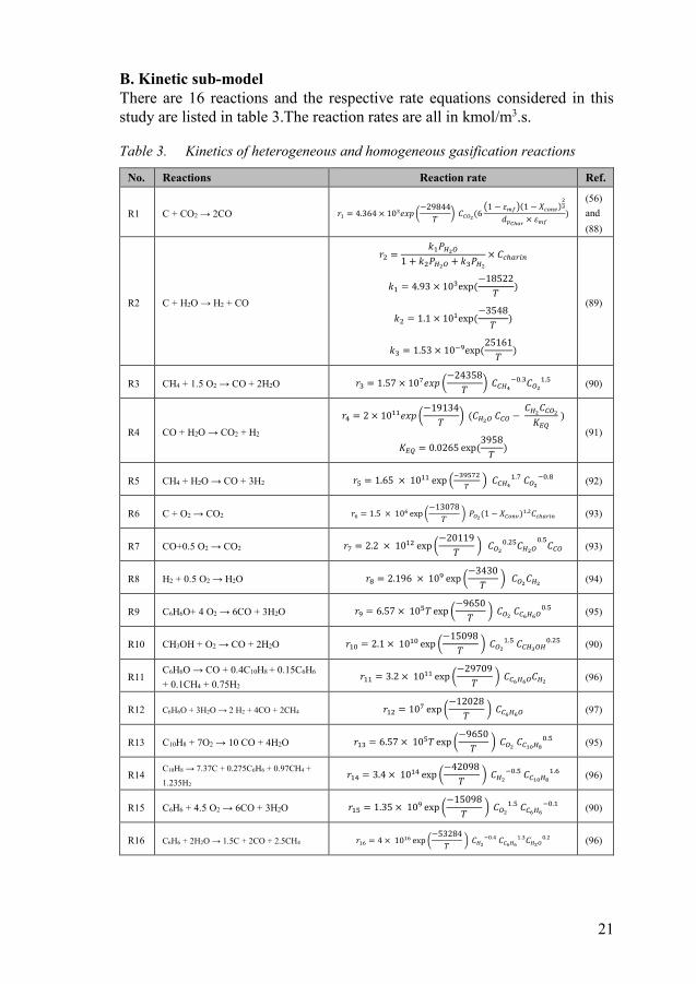
B. Kinetic sub-model There are 16 reactions and the respective rate equations considered in this study are listed in table 3.The reaction rates are all in kmol/m3.s.

Table 3. Kinetics of heterogeneous and homogeneous gasification reactions

No. Reactions Reaction rate Ref.

R1 C + CO2 → 2CO 𝑟𝑟1 = 4.364 × 103𝑒𝑒𝑒𝑒𝑒𝑒 (−29844𝑇𝑇 ) 𝐶𝐶𝐶𝐶𝐶𝐶2(6

(1 − 𝜀𝜀𝑚𝑚𝑚𝑚)(1 − 𝑋𝑋𝑐𝑐𝑐𝑐𝑐𝑐𝑐𝑐)23

𝑑𝑑𝑝𝑝𝐶𝐶ℎ𝑎𝑎𝑎𝑎 × 𝜀𝜀𝑚𝑚𝑚𝑚)

(56) and (88)

R2 C + H2O → H2 + CO

𝑟𝑟2 =𝑘𝑘1𝑃𝑃𝐻𝐻2𝐶𝐶

1 + 𝑘𝑘2𝑃𝑃𝐻𝐻2𝐶𝐶 + 𝑘𝑘3𝑃𝑃𝐻𝐻2× 𝐶𝐶𝑐𝑐ℎ𝑎𝑎𝑎𝑎𝑎𝑎𝑐𝑐

𝑘𝑘1 = 4.93 × 103exp (−18522𝑇𝑇 )

𝑘𝑘2 = 1.1 × 101exp (−3548𝑇𝑇 )

𝑘𝑘3 = 1.53 × 10−9exp (25161𝑇𝑇 )

(89)

R3 CH4 + 1.5 O2 → CO + 2H2O 𝑟𝑟3 = 1.57 × 107𝑒𝑒𝑒𝑒𝑒𝑒 (−24358𝑇𝑇 ) 𝐶𝐶𝐶𝐶𝐻𝐻4

−0.3𝐶𝐶𝐶𝐶21.5 (90)

R4 CO + H2O → CO2 + H2

𝑟𝑟4 = 2 × 1011𝑒𝑒𝑒𝑒𝑒𝑒 (−19134𝑇𝑇 ) (𝐶𝐶𝐻𝐻2𝐶𝐶 𝐶𝐶𝐶𝐶𝐶𝐶 −

𝐶𝐶𝐻𝐻2𝐶𝐶𝐶𝐶𝐶𝐶2𝐾𝐾𝐸𝐸𝐸𝐸

)

𝐾𝐾𝐸𝐸𝐸𝐸 = 0.0265 exp(3958𝑇𝑇 )

(91)

R5 CH4 + H2O → CO + 3H2 𝑟𝑟5 = 1.65 × 1011 exp (−39572𝑇𝑇 ) 𝐶𝐶𝐶𝐶𝐻𝐻4

1.7 𝐶𝐶𝐶𝐶2−0.8 (92)

R6 C + O2 → CO2 𝑟𝑟6 = 1.5 × 106 exp (−13078𝑇𝑇 ) 𝑃𝑃𝐶𝐶2(1 − 𝑋𝑋𝐶𝐶𝑐𝑐𝑐𝑐𝑐𝑐 )1.2𝐶𝐶𝑐𝑐ℎ𝑎𝑎𝑎𝑎𝑎𝑎𝑐𝑐 (93)

R7 CO+0.5 O2 → CO2 𝑟𝑟7 = 2.2 × 1012 exp (−20119𝑇𝑇 ) 𝐶𝐶𝐶𝐶2

0.25𝐶𝐶𝐻𝐻2𝐶𝐶0.5𝐶𝐶𝐶𝐶𝐶𝐶 (93)

R8 H2 + 0.5 O2 → H2O 𝑟𝑟8 = 2.196 × 109 exp (−3430𝑇𝑇 ) 𝐶𝐶𝐶𝐶2𝐶𝐶𝐻𝐻2 (94)

R9 C6H6O+ 4 O2 → 6CO + 3H2O 𝑟𝑟9 = 6.57 × 105𝑇𝑇 exp (−9650𝑇𝑇 ) 𝐶𝐶𝐶𝐶2 𝐶𝐶𝐶𝐶6𝐻𝐻6𝐶𝐶

0.5 (95)

R10 CH3OH + O2 → CO + 2H2O 𝑟𝑟10 = 2.1 × 1010 exp (−15098𝑇𝑇 ) 𝐶𝐶𝐶𝐶2

1.5 𝐶𝐶𝐶𝐶𝐻𝐻3𝐶𝐶𝐻𝐻0.25 (90)

R11 C6H6O → CO + 0.4C10H8 + 0.15C6H6 + 0.1CH4 + 0.75H2

𝑟𝑟11 = 3.2 × 1011 exp (−29709𝑇𝑇 ) 𝐶𝐶𝐶𝐶6𝐻𝐻6𝐶𝐶𝐶𝐶𝐻𝐻2 (96)

R12 C6H6O + 3H2O → 2 H2 + 4CO + 2CH4 𝑟𝑟12 = 107 exp (−12028𝑇𝑇 ) 𝐶𝐶𝐶𝐶6𝐻𝐻6𝐶𝐶 (97)

R13 C10H8 + 7O2 → 10 CO + 4H2O 𝑟𝑟13 = 6.57 × 105𝑇𝑇 exp (−9650𝑇𝑇 ) 𝐶𝐶𝐶𝐶2 𝐶𝐶𝐶𝐶10𝐻𝐻8

0.5 (95)

R14 C10H8 → 7.37C + 0.275C6H6 + 0.97CH4 +

1.235H2 𝑟𝑟14 = 3.4 × 1014 exp (−42098

𝑇𝑇 ) 𝐶𝐶𝐻𝐻2−0.5 𝐶𝐶𝐶𝐶10𝐻𝐻8

1.6 (96)

R15 C6H6 + 4.5 O2 → 6CO + 3H2O 𝑟𝑟15 = 1.35 × 109 exp (−15098𝑇𝑇 ) 𝐶𝐶𝐶𝐶2

1.5 𝐶𝐶𝐶𝐶6𝐻𝐻6−0.1 (90)

R16 C6H6 + 2H2O → 1.5C + 2CO + 2.5CH4 𝑟𝑟16 = 4 × 1016 exp (−53284𝑇𝑇 ) 𝐶𝐶𝐻𝐻2

−0.4 𝐶𝐶𝐶𝐶6𝐻𝐻61.3𝐶𝐶𝐻𝐻2𝐶𝐶

0.2 (96)

22

C. Hydrodynamic sub-model Except for the kinetic-only case, in the rest of the cases hydrodynamic equa-tions for solid particles in the fluidized beds are also included. The common hydrodynamic equations which have been used in both TPT and CCBM mod-els and the specific hydrodynamic equations used in the hydrodynamic sub-model of TPT and CCBM models are shown in table 4.

Table 4. Equations used in different hydrodynamic sub-models in this study

Common parameters in hydrodynamic models Ref.

Minimum fluidization velocity 𝑢𝑢𝑚𝑚𝑚𝑚 = 33.7𝜇𝜇

𝜌𝜌𝑔𝑔𝑑𝑑𝑝𝑝𝐶𝐶ℎ𝑎𝑎𝑎𝑎 √1 + 3.59 × 10−5𝐴𝐴𝐴𝐴 − 1

𝐴𝐴𝐴𝐴 =𝑑𝑑𝑝𝑝𝐶𝐶ℎ𝑎𝑎𝑎𝑎

3𝜌𝜌𝑔𝑔(𝜌𝜌𝑠𝑠 − 𝜌𝜌𝑔𝑔)𝑔𝑔𝜇𝜇2

(62)

Bubble velocity 𝑢𝑢𝑏𝑏 = 𝑢𝑢 − 𝑢𝑢𝑚𝑚𝑚𝑚 + 𝑢𝑢𝑏𝑏𝑏𝑏

𝑢𝑢𝑏𝑏𝑏𝑏 = 0.711√𝑔𝑔𝑑𝑑𝑏𝑏 (98)

Bubble diameter

𝑑𝑑𝑏𝑏 = 𝑑𝑑𝑏𝑏𝑚𝑚 + (𝑑𝑑𝑏𝑏0 − 𝑑𝑑𝑏𝑏𝑚𝑚)𝑒𝑒−0.3ℎ/𝑑𝑑𝑏𝑏𝑏𝑏𝑏𝑏

𝑑𝑑𝑏𝑏𝑚𝑚 = 0.652[𝐴𝐴𝑏𝑏𝑏𝑏𝑑𝑑(𝑢𝑢 − 𝑢𝑢𝑚𝑚𝑚𝑚)]0.4

𝑑𝑑𝑏𝑏0 = 0.347[𝐴𝐴𝑏𝑏𝑏𝑏𝑑𝑑(𝑢𝑢 − 𝑢𝑢𝑚𝑚𝑚𝑚)/𝑛𝑛𝑜𝑜𝑏𝑏𝑚𝑚]0.4

𝑖𝑖𝑖𝑖 5 ≤ 𝑢𝑢 ≤ 50 𝑐𝑐𝑐𝑐𝑠𝑠

7.9 ≤ 𝑑𝑑𝑏𝑏𝑏𝑏𝑑𝑑 ≤ 100 𝑐𝑐𝑐𝑐

(98)

Bubble to emulsion gas interchange coefficient

𝐾𝐾𝑏𝑏𝑏𝑏 = 4.5 (𝑢𝑢𝑏𝑏𝑑𝑑𝑏𝑏

) + 5.85 (𝐷𝐷𝐴𝐴𝐴𝐴0.5𝑔𝑔1/4

𝑑𝑑𝑏𝑏5/4 )

𝐾𝐾𝑏𝑏𝑏𝑏 = 6.77 (𝐷𝐷𝐴𝐴𝐴𝐴𝜀𝜀𝑏𝑏𝑢𝑢𝑏𝑏𝑏𝑏 𝑑𝑑𝑏𝑏

3 )0.5

1𝐾𝐾𝑏𝑏𝑏𝑏

= 1𝐾𝐾𝑏𝑏𝑏𝑏

+ 1𝐾𝐾𝑏𝑏𝑏𝑏

(62)

Two phase structure model

Emulsion phase 𝑑𝑑𝐶𝐶𝐴𝐴𝑏𝑏

𝑑𝑑𝑑𝑑 = 𝐴𝐴𝐴𝐴𝑏𝑏(1 − 𝜀𝜀𝑏𝑏)(1 − 𝛿𝛿) + 𝐾𝐾𝑏𝑏𝑏𝑏𝛿𝛿(𝐶𝐶𝐴𝐴𝑏𝑏 − 𝐶𝐶𝐴𝐴𝑏𝑏)𝑢𝑢𝑏𝑏(1 − 𝛿𝛿)

(63)

Bubble phase 𝑑𝑑𝐶𝐶𝐴𝐴𝑏𝑏

𝑑𝑑𝑑𝑑 = 𝐴𝐴𝐴𝐴𝑏𝑏(1 − 𝜀𝜀𝑏𝑏) − 𝐾𝐾𝑏𝑏𝑏𝑏𝛿𝛿(𝐶𝐶𝐴𝐴𝑏𝑏 − 𝐶𝐶𝐴𝐴𝑏𝑏)𝑢𝑢𝑏𝑏

Average emulsion voidage 𝜀𝜀𝑏𝑏 = 𝜀𝜀𝑚𝑚𝑚𝑚 + 0.00061 𝑒𝑒(𝑢𝑢−𝑢𝑢𝑚𝑚𝑚𝑚0.262 )

Average bubble voidage 𝜀𝜀𝑏𝑏 = 0.784 − 0.139 𝑒𝑒(−𝑢𝑢−𝑢𝑢𝑚𝑚𝑚𝑚0.272 )

Bubble fraction 𝛿𝛿 = 1 − 𝑒𝑒(−𝑢𝑢−𝑢𝑢𝑚𝑚𝑚𝑚

0.62 )

Emulsion velocity 𝑢𝑢𝑏𝑏 = 𝑢𝑢 − 𝛿𝛿𝑢𝑢𝑏𝑏1 − 𝛿𝛿

Counter current back mixing model

Char balance in ascending phase 𝑑𝑑𝐶𝐶𝑎𝑎𝑠𝑠,𝑏𝑏

𝑑𝑑𝑑𝑑 = [𝐾𝐾𝑤𝑤(𝐶𝐶𝑎𝑎𝑠𝑠,𝑏𝑏 − 𝐶𝐶𝑑𝑑𝑠𝑠,𝑏𝑏) 𝑖𝑖𝑎𝑎𝑠𝑠 − 𝑖𝑖𝑎𝑎𝑠𝑠 𝐴𝐴𝑏𝑏]/𝑢𝑢𝑎𝑎𝑠𝑠 (30)

Char balance in descending phase

𝑑𝑑𝐶𝐶𝑑𝑑𝑠𝑠,𝑏𝑏𝑑𝑑𝑑𝑑 = [𝐾𝐾𝑤𝑤(𝐶𝐶𝑑𝑑𝑠𝑠,𝑏𝑏 − 𝐶𝐶𝑎𝑎𝑠𝑠,𝑏𝑏) 𝑖𝑖𝑎𝑎𝑠𝑠 − 𝑖𝑖𝑑𝑑𝑠𝑠 𝐴𝐴𝑏𝑏]/𝑢𝑢𝑑𝑑𝑠𝑠

𝑢𝑢𝑎𝑎𝑠𝑠 = 𝑢𝑢𝑑𝑑𝑠𝑠𝑖𝑖𝑑𝑑𝑠𝑠 /𝑖𝑖𝑎𝑎𝑠𝑠

𝐾𝐾𝑤𝑤 = 0.0812𝜀𝜀𝑚𝑚𝑚𝑚𝑑𝑑𝑏𝑏

(30)

(30)

(99)

23

3.4 Principal component analysis (PCA), Partial least square (PLS) and Genetic algorithms (GA)

Multivariate analysis of the experimental dataset with data from several dif-ferent CFB gasifiers is performed in two steps in order to address RQ1 and partly RQ2. The first step uses the principal component analysis (PCA) ap-proach to determine the existing interrelations between input and output pa-rameters in biomass gasification. The second step develops an empirical model using the partial least square regression (PLS-R) approach. This is fur-ther explained in the appended paper V.

PCA is a statistical projection method (68) in which the data matrix is pre-sented in multidimensional space by points and is defined by the variables as the axis in this space. Basically, PCA forms a line that is called the principal component (PC) in the direction that data points have the highest possible var-iance. Other PCs (PC2, PC3, PC4, etc.) are formed orthogonal to the preceding PCs showing the next highest variances. The loadings plot, which is formed based on the PCs, illustrates existing correlations between input and output parameters. In the loadings plot, the inner circle indicates 50% of explained variance and the outer circle indicates 100% of explained variance (100).

Additionally, PLS-R considers the causality relation between input (X) and output (Y) parameters, and accordingly estimates the relationship between in-dependent X and dependent Y variables. This method is based on determining PCs in the input parameter data matrix to predict the PCs in the output param-eter data matrix. Using this method requires prior normalization and scaling of the data. In this thesis, binary dummy variables (-1,+1) are created in order to include the impact of categorical variables (such as bed material) in quan-titative analysis. +1 stands for the existence of a category while -1 is used when the category does not exist. (68). PLS-R forms a linear regression equa-tion that links input parameters to the output parameters. As shown in equation (3), (b1, b2, …, bn) are regression coefficients and (b0) is the Y intercept.

𝑌𝑌 = 𝑏𝑏0 + 𝑏𝑏1𝑋𝑋1 + 𝑏𝑏2𝑋𝑋2 + ⋯+ 𝑏𝑏𝑛𝑛𝑋𝑋𝑛𝑛 (3)

In order to determine the parameters with the most significant impact on bio-mass gasification and to address RQ2, the uncertainty test is applied on the regression coefficients of the empirical PLS model. The results are shown in the form of p-values that express the significance level (5% in this study). Therefore any parameter with p-value<0.05 is considered as significant (101).

Finally, in order to determine the optimal operation condition window for fluidized bed gasifiers as a part of the knowledge gained in the process of addressing RQ1 and RQ2, the GA is applied as an optimization tool using the Matlab global optimization tool box (102). GA was developed in the early 1970s by Holland et al (103), and is a well-known optimization technique. This method is usually used for complex engineering problems (104,105), and

24

is inspired by principles of natural evolution such as mutation, selection and crossing over. GA is more suitable for finding global optimal solutions spe-cifically for multi-objectives optimization problems than for other conven-tional optimization methods (106).

Objective functions, decision variables and the constraints considered in this thesis are shown in the following statements (S-1 to S-3):

𝑂𝑂𝑂𝑂𝑂𝑂𝑂𝑂𝑂𝑂𝑂𝑂𝑂𝑂𝑂𝑂𝑂𝑂 𝑓𝑓𝑓𝑓𝑓𝑓𝑂𝑂𝑂𝑂𝑂𝑂𝑓𝑓𝑓𝑓𝑓𝑓

{

𝑀𝑀𝑀𝑀𝑀𝑀𝑂𝑂𝑀𝑀𝑂𝑂𝑀𝑀𝑂𝑂: 𝑉𝑉𝑓𝑓𝑉𝑉𝑓𝑓𝑀𝑀𝑂𝑂 𝑓𝑓𝑓𝑓𝑀𝑀𝑂𝑂𝑂𝑂𝑂𝑂𝑓𝑓𝑓𝑓 𝑓𝑓𝑓𝑓𝐶𝐶𝐶𝐶4 (%)

𝑉𝑉𝑓𝑓𝑉𝑉𝑓𝑓𝑀𝑀𝑂𝑂 𝑓𝑓𝑓𝑓𝑀𝑀𝑂𝑂𝑂𝑂𝑂𝑂𝑓𝑓𝑓𝑓 𝑓𝑓𝑓𝑓 𝐶𝐶2 (%)𝑉𝑉𝑓𝑓𝑉𝑉𝑓𝑓𝑀𝑀𝑂𝑂 𝑓𝑓𝑓𝑓𝑀𝑀𝑂𝑂𝑂𝑂𝑂𝑂𝑓𝑓𝑓𝑓 𝑓𝑓𝑓𝑓 𝐶𝐶𝑂𝑂 (%), 𝑉𝑉𝑓𝑓𝑉𝑉𝑓𝑓𝑀𝑀𝑂𝑂 𝑓𝑓𝑓𝑓𝑀𝑀𝑂𝑂𝑂𝑂𝑂𝑂𝑓𝑓𝑓𝑓 𝑓𝑓𝑓𝑓𝐶𝐶2𝐶𝐶4 (%), 𝐶𝐶𝑀𝑀𝑓𝑓𝑂𝑂𝑓𝑓𝑓𝑓 𝑂𝑂𝑓𝑓𝑓𝑓𝑂𝑂𝑂𝑂𝑓𝑓𝑓𝑓𝑂𝑂𝑓𝑓𝑓𝑓 (%),

𝐿𝐿𝐶𝐶𝑉𝑉 𝑓𝑓𝑓𝑓 𝑂𝑂ℎ𝑂𝑂 𝑝𝑝𝑓𝑓𝑓𝑓𝑝𝑝𝑓𝑓𝑂𝑂𝑂𝑂 𝑔𝑔𝑀𝑀𝑓𝑓 (𝑀𝑀𝑀𝑀𝑚𝑚3)

𝑝𝑝𝑓𝑓𝑑𝑑 𝑔𝑔𝑀𝑀𝑓𝑓 𝑑𝑑𝑂𝑂𝑂𝑂𝑉𝑉𝑝𝑝 (𝑚𝑚3

𝑘𝑘𝑘𝑘) 𝑀𝑀𝑂𝑂𝑓𝑓𝑂𝑂𝑀𝑀𝑂𝑂𝑀𝑀𝑂𝑂: 𝑉𝑉𝑓𝑓𝑉𝑉𝑓𝑓𝑀𝑀𝑂𝑂 𝑓𝑓𝑓𝑓𝑀𝑀𝑂𝑂𝑂𝑂𝑂𝑂𝑓𝑓𝑓𝑓 𝑓𝑓𝑓𝑓 𝐶𝐶𝑂𝑂2 (%) 𝑂𝑂𝑀𝑀𝑓𝑓 𝑑𝑑𝑂𝑂𝑂𝑂𝑉𝑉𝑝𝑝 ( 𝑘𝑘

𝑛𝑛𝑚𝑚3)

(S-1)

𝐷𝐷𝑂𝑂𝑂𝑂𝑂𝑂𝑓𝑓𝑂𝑂𝑓𝑓𝑓𝑓 𝑂𝑂𝑀𝑀𝑓𝑓𝑂𝑂𝑀𝑀𝑂𝑂𝑉𝑉𝑂𝑂𝑓𝑓

{

𝐸𝐸𝐸𝐸 𝑂𝑂𝑀𝑀𝑉𝑉𝑓𝑓𝑂𝑂

𝑃𝑃𝑀𝑀𝑓𝑓𝑂𝑂𝑂𝑂𝑂𝑂𝑉𝑉𝑂𝑂 𝑓𝑓𝑂𝑂𝑀𝑀𝑂𝑂 (𝑀𝑀𝑀𝑀)𝑀𝑀𝑓𝑓𝑂𝑂𝑓𝑓𝑂𝑂𝑓𝑓𝑓𝑓𝑂𝑂 𝑂𝑂𝑓𝑓𝑓𝑓𝑂𝑂𝑂𝑂𝑓𝑓𝑂𝑂 (%)

𝑆𝑆𝐵𝐵 𝑓𝑓𝑀𝑀𝑂𝑂𝑂𝑂𝑓𝑓

𝐵𝐵𝑂𝑂𝑝𝑝 𝑀𝑀𝑀𝑀𝑂𝑂𝑂𝑂𝑓𝑓𝑂𝑂𝑀𝑀𝑉𝑉 (𝑆𝑆𝑂𝑂𝑉𝑉𝑂𝑂𝑂𝑂𝑀𝑀 𝑓𝑓𝑀𝑀𝑓𝑓𝑝𝑝, 𝐷𝐷𝑓𝑓𝑉𝑉𝑓𝑓𝑀𝑀𝑂𝑂𝑂𝑂𝑂𝑂 𝑀𝑀𝑓𝑓𝑝𝑝 𝑂𝑂𝑉𝑉𝑂𝑂𝑂𝑂𝑂𝑂𝑓𝑓𝑂𝑂)

(S-2)

𝐶𝐶𝑓𝑓𝑓𝑓𝑓𝑓𝑂𝑂𝑓𝑓𝑀𝑀𝑂𝑂𝑓𝑓𝑂𝑂𝑓𝑓

{

0.17 ≤ 𝐸𝐸𝐸𝐸 𝑂𝑂𝑀𝑀𝑉𝑉𝑓𝑓𝑂𝑂 ≤ 0.73

0.1 ≤ 𝑃𝑃𝑀𝑀𝑓𝑓𝑂𝑂𝑂𝑂𝑂𝑂𝑉𝑉𝑂𝑂 𝑓𝑓𝑂𝑂𝑀𝑀𝑂𝑂 ≤ 10.253.5 ≤ 𝑀𝑀𝑓𝑓𝑂𝑂𝑓𝑓𝑂𝑂𝑓𝑓𝑓𝑓𝑂𝑂 𝑂𝑂𝑓𝑓𝑓𝑓𝑂𝑂𝑂𝑂𝑓𝑓𝑂𝑂 ≤ 22

0 ≤ 𝑆𝑆𝐵𝐵 𝑓𝑓𝑀𝑀𝑂𝑂𝑂𝑂𝑓𝑓 ≤ 1.45

𝐵𝐵𝑂𝑂𝑝𝑝 𝑀𝑀𝑀𝑀𝑂𝑂𝑂𝑂𝑓𝑓𝑂𝑂𝑀𝑀𝑉𝑉 = −1 𝑓𝑓𝑓𝑓 + 1

(S-3)

Decision variables are chosen based on the results of multivariate analysis on the dataset. These parameters not only have the most significant impact but also show opposite impact on the output parameters (showing positive impact on some output components while having negative impact on other output pa-rameters). This is further explained in the results section (see 4.3). It is im-portant to note that the parameters that are not listed in the constraints are considered fixed-value parameters. The values of the fixed parameters are the average values of the range shown in the data matrix. The upper and lower bounds that are assigned to the decision variables in (S-3) are based on the range presented for them in the data set in paper V. The data matrix is explic-itly presented in paper V. The gasifiers used to form the dataset are listed in table 5 as CFB 1-8 and 10, in the results section (see 4.1)

25

3.5 Model evaluation In order to evaluate the performance of different models that are investigated in this thesis, different evaluating factors have been introduced.

The relative error for each component at each data point (rel Eij) is calcu-lated by equation 4 while the average relative error for overall model evalua-tion of each component (rel Ei) in the gas is calculated by equation 5. i stands for each component at each set point and j represent each set point:

𝑟𝑟𝑟𝑟𝑟𝑟 𝐸𝐸𝑖𝑖𝑖𝑖 = |𝑦𝑦𝑖𝑖𝑖𝑖−𝑦𝑦𝑖𝑖𝑖𝑖𝑦𝑦𝑖𝑖𝑖𝑖

| (4)

𝑟𝑟𝑟𝑟𝑟𝑟 𝐸𝐸𝑖𝑖 = (∑ 𝑟𝑟𝑟𝑟𝑟𝑟 𝐸𝐸𝑖𝑖𝑖𝑖)/𝑛𝑛𝑛𝑛𝑖𝑖=1 (5)

where yie and yip are the experimental and predicted results, respectively. one set of gas composition (volume fraction of CO, CO2, H2, CH4 and tar)

is produced at each set point, which comprises of a single set of values for ER, S/B ratio, temperature, pressure and load. The error calculated at each set point is called the overall error at that set point (OEj). OEj is also calcu-lated and considered as the basis for estimation of model accuracy.

𝑂𝑂𝐸𝐸𝑖𝑖 = ∑ (𝑟𝑟𝑟𝑟𝑟𝑟 𝐸𝐸𝑖𝑖𝑖𝑖 ×𝑛𝑛𝑖𝑖=1 𝑦𝑦𝑖𝑖𝑖𝑖) (6)

Additional indexes are introduced in order to evaluate the performance of dif-ferent models over a range of set points. These are average overall error (OE) and variation width (VW). OE identifies the level of accuracy, whereas VW shows the extent to which the changes of other parameters can influence the accuracy of the model when a parameter is fixed. The smaller the VW at a fixed parameter, the lower the level of impact of the other parameters on the model performance. These are calculated as follows:

𝑂𝑂𝐸𝐸 = (∑ 𝑂𝑂𝐸𝐸𝑖𝑖)/𝑛𝑛𝑛𝑛𝑖𝑖=1 (7)

where n represents the number of set points in the analyzed dataset.

𝑉𝑉𝑉𝑉 = 𝑂𝑂𝐸𝐸𝑖𝑖𝑗𝑗𝑗𝑗𝑗𝑗 − 𝑂𝑂𝐸𝐸𝑖𝑖𝑗𝑗𝑖𝑖𝑛𝑛 (8)

OEjmin and OEjmax are the minimum and maximum values of OEj in the ana-lyzed dataset, respectively.

The approaches used for validation of the models are R2 and RMSEP. Equa-tions (9) and (10) show how these are calculated. Generally, when comparing the predicted results with experimental data in the evaluation of the model, R2

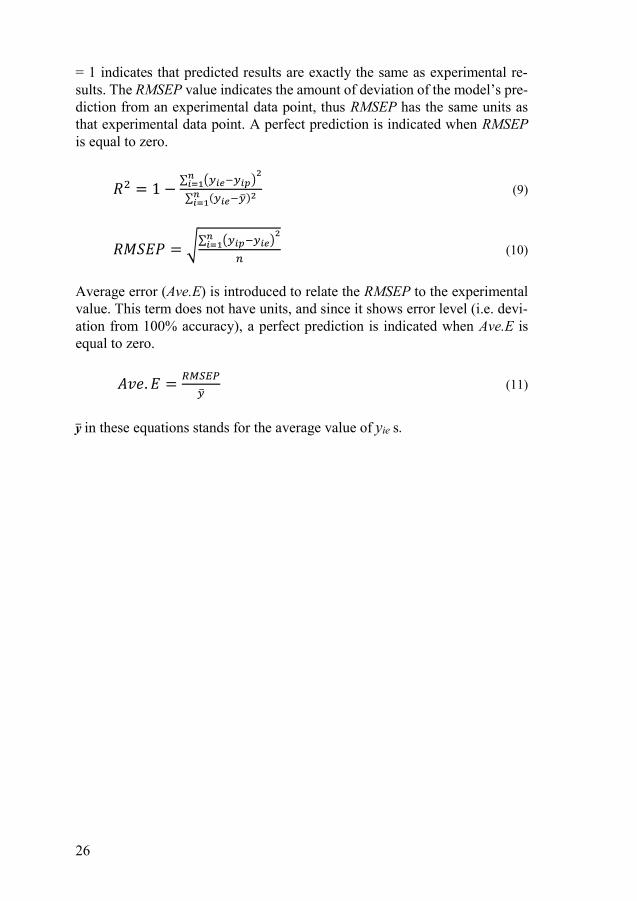
26

= 1 indicates that predicted results are exactly the same as experimental re-sults. The RMSEP value indicates the amount of deviation of the model’s pre-diction from an experimental data point, thus RMSEP has the same units as that experimental data point. A perfect prediction is indicated when RMSEP is equal to zero.

𝑅𝑅2 = 1 − ∑ (𝑦𝑦𝑖𝑖𝑖𝑖−𝑦𝑦𝑖𝑖𝑖𝑖)2𝑛𝑛

𝑖𝑖=1∑ (𝑦𝑦𝑖𝑖𝑖𝑖−��𝑦)2𝑛𝑛𝑖𝑖=1

(9)

𝑅𝑅𝑅𝑅𝑅𝑅𝑅𝑅𝑅𝑅 = √∑ (𝑦𝑦𝑖𝑖𝑖𝑖−𝑦𝑦𝑖𝑖𝑖𝑖)2𝑛𝑛

𝑖𝑖=1𝑛𝑛 (10)

Average error (Ave.E) is introduced to relate the RMSEP to the experimental value. This term does not have units, and since it shows error level (i.e. devi-ation from 100% accuracy), a perfect prediction is indicated when Ave.E is equal to zero.

𝐴𝐴𝐴𝐴𝐴𝐴. 𝑅𝑅 = 𝑅𝑅𝑅𝑅𝑅𝑅𝑅𝑅𝑅𝑅��𝑦 (11)

y in these equations stands for the average value of yie s.

27

4 Results and Discussion

4.1 Collected experimental data from different types of gasifiers

In order to address RQ1, the experimental data has been collected from dif-ferent types of gasifiers to validate and evaluate the theoretical and semi-em-pirical models, and to form the data set required for developing the empirical model. Also to address RQ2, data from different types of fluidized bed gasi-fiers are needed. Table 5 presents the experimental setups from which data has been collected and used for the purposes mentioned. These data have been collected during the time from published literature and through direct contact with the authors in some cases, mainly for fluidized bed gasifiers. Therefore not all of them have been used during the assessment of different types of gasifiers which is presented in paper I. In order to form figure 2 and 3 only following gasifiers from table 5 are considered; BFB 1-3 and 5, CFB 3-5 and 10, downdraft 1-3 and entrained-down flow 1-3.

28

Table 5. Experimental data different gasifiers investigated in this thesis

Type of gasifiers Feedstock Temp. (0C)

Pressure (bar)

ER S/B Ref

BFB 1 Pine sawdust 800 1 0.26–0.37 0 (6) BFB 2 Crushed wood

pellets 782–824 1.5–5.1 0.3–0.51 0 (107)

BFB 3 Pine sawdust 700–900 1 0.19–0.27 0–1.56 (85) BFB 4 Beech wood 740–755 1 0.13–0.48 0 (30) BFB 5 Sawdust 750–950 1 0.18–0.37 1.7 (84) BFB 6 Woody biomass 800 1 0.19–0.32 0 (52) BFB 7 Natural wood

and wood waste 768-945 1 0.13-0.31 0.62 (86)

BFB 8 Wood chips 740-857 1 0.27-0.33 0 (23) BFB 9 Olive kernels 750-850 1 0.2-0.4 0 (108) BFB 10 Coir pitch, rice

husk and sawdust 750-880 1 0.3-0.5 0 (109)

BFB 11 Palm kernel shell and coconut shell

700-900 1 0.15-0.3 0 (110)

CFB 1 Agrol, willow 770–820 1 0.35–0.39 0.9–1.45 (50) CFB 2 Rice husk 688–784 1 0.22–0.3 0 (74) CFB 3 Different bio-

mass 803–855 1 0.32–0.43 0 (75)

CFB 4 Gum wood 686–919 1 0.17–0.22 0 (83) CFB 5 Leached Orujillo 780–800 1 0.41–0.59 0 (111) CFB 6 Cypress and

Hemlock 701–815 1.19 0.22–0.54 0–0.95 (48)

CFB 7 Cane trash 850 1 0.215–0.3 0 (112) CFB 8 Sunflower,

Jatropha and wil-low

750-800 1 0.3 0 (77)

CFB 9 Black liquor (BL)

667–727 1 0.35–0.4 0 (82)

CFB 10 Sawdust 735–890 4–5 0.28–0.43 0.08–0.59 (113) CFB 11 Coir pitch 650-1020 1 0.18-0.31 0 (114) Downdraft fixed bed 1

Wood pellets 800 1 0.22–0.26 0 (115)

Downdraft fixed bed 2

Hazelnut shell 820–1021 1 0.32–0.4 0 (116)

Downdraft fixed bed 3

Wood chips 700 1 0.26–0.46 0 (40)

Entrained –down flow 1

Rice husk, Sawdust

1000–1400

1 0.02–0.82 0 (117)

Entrained –down flow 2

Rice husk 700–1000 1 0.22–0.34 0 (118)

Entrained –down flow 3

Pulverized wood 627–1227 1 0.12–0.2 0 (119)

29

Figure 2 shows the volume fraction of CH4 in the product gas at different ER values for BFB, CFB, entrained flow and downdraft fixed bed gasifiers which are presented in table 5 (BFB 1-6, CFB 1-7 & 10, entrained flow 1-3 and downdraft 1-3). The scattered points show the experimental data points while the lines are only used for clearer visual presentation of the data. Figure 2 shows that CH4 content in the product gas is the highest for CFB gasifiers and the lowest in the entrained flow gasifier. At lower ER values, CH4 content is higher since increasing ER value and thus shifting gasification towards com-bustion decreases CH4 content, dramatically. Therefore, if the aim is to obtain high methane content in the product gas, the fluidized bed gasifier operating with ER values lower than 0.35 is suitable.

Figure 3 shows a comparison of different types of gasifiers according to heat-ing value of the product gas at different ER values. This figure also shows that with ER values between 0.1-0.4, which are typical for gasification, fluidized bed gasifiers produce gases with higher heating value compared to fixed bed and entrained flow gasifiers.

The results of this section highlights the advantages of using fluidized bed gasifiers (CFB and BFB) for gasification of biomass. Further in this thesis modeling and simulation of this specific type of gasifier is studied in detail.

Figure 2. Changes in volume fraction of CH4 in dry product gas from different ty-pes of gasifiers at different ER values

30

4.2 General model for biomass gasification for system-level analysis

As mentioned in literature review (section 2.3), three different approaches are available to address RQ1 and develop a general and accurate model for biomass gasification: theoretical models, semi-empirical models and empiri-cal models. In this section the results of considering each approach are pre-sented. Results are taken from papers II, III, IV and V.

4.2.1 Theoretical model (Equilibrium model) Figure 4 shows the product gas composition (H2, CO, CO2 and CH4) predicted by the simulations performed in Aspen Plus on black liquor gasification using the EM compared to the experimental data from CFB 9 (82) in table 5. These results are taken from paper II. However, since paper II was published, more experimental points have been collected and more knowledge has been gained on the black liquor gasification plant (82). Figure 5 shows results based on the more recent Aspen Plus simulation on this gasifier. The data in figure 5 is not presented in any of the appended papers.

Figure 4 shows that the EM underestimates the volume fractions of CO2 and CH4, and that the error in the prediction decreases at ER values greater

Figure 3. Changes in lower heating value (LHV) of the product gas from different types of gasifiers at different equivalence ratio (ER) values

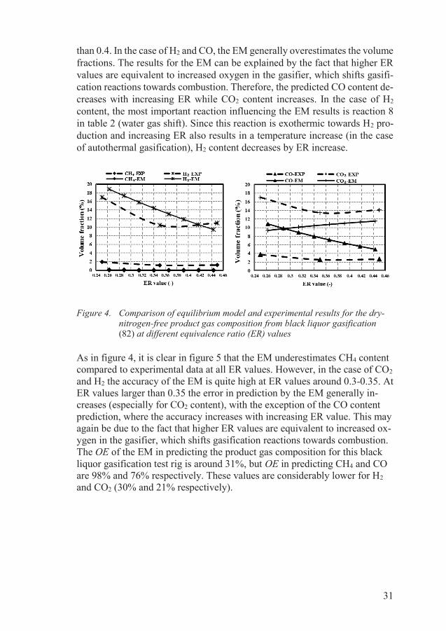
31

than 0.4. In the case of H2 and CO, the EM generally overestimates the volume fractions. The results for the EM can be explained by the fact that higher ER values are equivalent to increased oxygen in the gasifier, which shifts gasifi-cation reactions towards combustion. Therefore, the predicted CO content de-creases with increasing ER while CO2 content increases. In the case of H2 content, the most important reaction influencing the EM results is reaction 8 in table 2 (water gas shift). Since this reaction is exothermic towards H2 pro-duction and increasing ER also results in a temperature increase (in the case of autothermal gasification), H2 content decreases by ER increase.

Figure 4. Comparison of equilibrium model and experimental results for the dry-nitrogen-free product gas composition from black liquor gasification (82) at different equivalence ratio (ER) values

As in figure 4, it is clear in figure 5 that the EM underestimates CH4 content compared to experimental data at all ER values. However, in the case of CO2 and H2 the accuracy of the EM is quite high at ER values around 0.3-0.35. At ER values larger than 0.35 the error in prediction by the EM generally in-creases (especially for CO2 content), with the exception of the CO content prediction, where the accuracy increases with increasing ER value. This may again be due to the fact that higher ER values are equivalent to increased ox-ygen in the gasifier, which shifts gasification reactions towards combustion. The OE of the EM in predicting the product gas composition for this black liquor gasification test rig is around 31%, but OE in predicting CH4 and CO are 98% and 76% respectively. These values are considerably lower for H2 and CO2 (30% and 21% respectively).

32

Figure 5. The recent comparison of equilibrium model and experimental results for

the dry-nitrogen free product gas composition (a) H2, (b) CH4, (c) CO and (d) CO2 from black liquor gasification (82) at different equivalence ratio (ER) values including more data points

The results shown in figures 4 and 5 show variable reliability and accuracy in the prediction by the EM, especially for CO and CH4 content. This indicates that the model needs modification to improve the accuracy of prediction. Pa-per III includes a systematic evaluation of the EM modification approaches, the results of which are presented below.

4.2.2 Semi-empirical model

4.2.2.1 Modified EMs Three main approaches available to improve the accuracy of prediction for the EM have been described in literature review and methodology sections (see 2.3 and 3.2). These models are:

(1) MODEL I: quasi-equilibrium temperature (QET) (2) MODEL II: empirical correlation for C-H components (3) MODEL III: reaction kinetics and in some cases also bed hydrodynamics.

33

The accuracy of these approaches in predicting gas composition for BFB 1, 5 and 6 (6,52,84) and CFB 1-4 (50,74,75,83), from table 5, are compared as explained above in methodology section (see section 3.2). The results pre-sented in figure 6 show that MODEL I shows the same overall error for both BFB and CFB gasifiers. This means that the gasifier specific design does not influence the accuracy of MODEL I. However, using MODEL II for CFBs and MODEL III for BFBs results in lower OE, because these models were originally developed for a CFB and a BFB gasifier, respectively. Thus the performance of the EM modified by the empirical and kinetic-hydrodynamic approaches is sensitive to the specific gasifier design. The sensitivity of the modified EMs to other operating parameters is addressed below

Figure 6. Average overall error level (OE) and variation for prediction of gas composition from bubbling fluidized bed (BFB) and circulating fluidized bed (CFB) gasifiers

Figure 7 is adapted from the results presented in paper III for cases in which one operating parameter is fixed value while the other operating parameters vary. The values for average overall error (OE) are shown by columns corre-sponding to the values on the left axis and variation width (VW) is shown by lines corresponding to the values on the right axis. As previously mentioned, for each fixed parameter, the model with the lowest OE and VW will be the most suitable model for that case, while also showing the highest sensitivity to the fixed parameter.

Figure 7(a) presents OE and VW of MODEL I, II and III at fixed values of ER (0.18, 0.22 and 0.38) while the other parameters are varied. Figure 7(b) presents the fixed load cases, figure 7(c) shows fixed temperature cases, and figure 7(d) shows cases with fixed S/B ratio.

Based on the results shown in figure 7, MODEL III has the smallest OE and VW compared to the other models when ER is fixed at 0.18 and 0.22. Since these values are for BFB gasifiers, and MODEL III was originally de-veloped for a BFB gasifier, it performs better than the other models for this

0

10

20

30

40

50

60

70

80

MODEL I MODEL II MODEL III

OE(

%

CFB gasifiers

0

10

20

30

40

50

60

70

80

MODEL I MODEL II MODEL III

OE

(%)

BFB gasifiers

34

condition. However, when ER = 0.38, the most accurate model is MODEL I, while MODEL II has the smallest VW. This means that MODEL II, which was developed for a CFB gasifier and is based on modifying the EM using empir-ical correlations with ER, is less influenced by the variation of the other pa-rameters when ER> 0.3. Based on the dataset used in this analysis, ER≥ 0.3 are typical for CFB gasifiers; therefore, less variation of results in this ER range is expected with MODEL II. However, MODEL I, in which the EM is modified by the QET method, shows better performance when T≤ 800 °C, which is associated with the same set points used for analysis at ER= 0.38. MODEL II shows the largest VW for all fixed temperature cases, which means that this model is more sensitive to the variation of other parameters at fixed temperature values. At T= 850 °C, that are taken from BFB gasifiers in this analysis, MODEL III shows the lowest OE and VW. This means that for BFB gasifiers with T> 800 °C, the variations of other parameters have less influ-ence on the performance of MODEL III than temperature changes.

Figure 7. Average overall error level (OE) and variation width (VW) in prediction of gas composition when (a) equivalence ratio (ER) value is fixed, (b) load is fixed, (c) temperature is fixed and (d) steam to biomass(S/B) ratio is fixed. In each case, other parameters than the fixed one are varying. The values for OE are shown by the columns and correspond to the left axis while VW is shown by lines matching the right axis.

(c)

0

10

20

30

40

50

60

70

80

0

10

20

30

40

50

60

70

80

0.18 0.22 0.38

VW

(%)

OE

(%)

ER value (-)

MODEL I MODEL IIMODEL III MODEL I-VWMODEL II-VW MODEL III-VW

0

10

20

30

40

50

60

70

80

0

10

20

30

40

50

60

70

80

0.241 0.273 0.354 0.407 0.438 1.942 1.951 2.219

VW

(%)

OE

(%)

Load (Mg.m-2.h-1)

MODEL I MODEL IIMODEL III MODEL I-VWMODEL II-VW MODEL III-VW

(a) (b)

0

10

20

30

40

50

60

70

80

0

10

20

30

40

50

60

70

80

780 800 850

VW

(%)

OE

(%)

Temperature (ºC)

MODEL I MODEL IIMODEL III MODEL I-VWMODEL II-VW MODEL III-VW

0

10

20

30

40

50

60

70

80

0

10

20

30

40

50

60

70

80

1.4 1.56 1.7 2.7

VW

(%)

OE

(%)

S/B ratio (-)

MODEL I MODEL IIMODEL III MODEL I-VWMODEL II-VW MODEL III-VW

(d)

35

When steam is used as a gasification agent, the variation of steam-to-biomass ratio (S/B) is important. MODEL II shows the largest OE which can be be-cause MODEL II was originally developed for air gasification in a CFB gasi-fier and the empirical correlations used for modification of the EM in this model are only relate to ER value. Moreover, the largest VW is for MODEL II when S/B=1.4 and 1.56. This shows that MODEL II is more sensitive to variation of other parameters than to S/B ratio. However, MODEL III shows the smallest OE and VW for all S/B ratios. This means that the performance of MODEL III is more sensitive to S/B ratio than the variation of other parame-ters. This is likely to be because MODEL III includes the kinetics of the water gas shift (WGS) reaction (see subsection 2.2) and consequently includes the impact of steam to product gas composition.

In addition to the operating parameters discussed above, the impact of load, as an index for the size of the reactor, is also examined. As shown in figure 7(b), with loads < 0.430 Mg/m2.h which represent BFB gasifiers in this anal-ysis, MODEL III shows the smallest OE and VW while MODEL II shows the largest OE and VW (except for load= 0.273 Mg/m2.h). The small VW in loads < 0.430 Mg/m2.h for MODEL III shows that variation of other operating pa-rameters are less effective than the application of fixed loads. However in the case of MODEL II, the impact due to changes in other parameters, when the load is < 0.430 Mg/m2.h, is more significant. MODEL III considers the hy-drodynamics of the bed and freeboard and is therefore highly sensitive to the size of the reactor. MODEL I shows the least variation and OE at T< 800 °C, which also corresponds to loads > 0.43 Mg/m2.h. This indicates that MODEL I is less sensitive to variations in parameters other than temperature and load in these ranges.

An overview of these observations and analyses is presented in table 6. MODEL I is limited by the temperature, and this temperature limit can be determined by trial-and-error. However, within its specific temperature range, it is flexible to different input parameters and the results show an acceptable level of accuracy (i.e. within ±30%) in those cases. This model however pro-duces large inaccuracies when steam is one of the gasification agents. The main modification in MODEL II is inclusion of the empirical correlation be-tween light hydrocarbons content and ER value, and the model is only accu-rate within the range of data used to derive the empirical correlations. In ad-dition, this model displays a high dependency on ER value and is therefore not applicable when ER> 0.44. Also it has low accuracy when ER< 0.3 (mainly observed for BFBs in this study). Conversely, the error level of MODEL III is quite low and acceptable for BFBs. However, it does not func-tion accurately for CFBs, large loads and temperatures other than the specific temperatures 700 °C, 750 °C, 800 °C, 850 °C and 900 °C.

Based on the general overview of these modification approaches, two new models, MOD-MODEL II and MOD-MODEL III are proposed. Since one of the major limitations of MODEL II is the strong impact of the specific gasifier

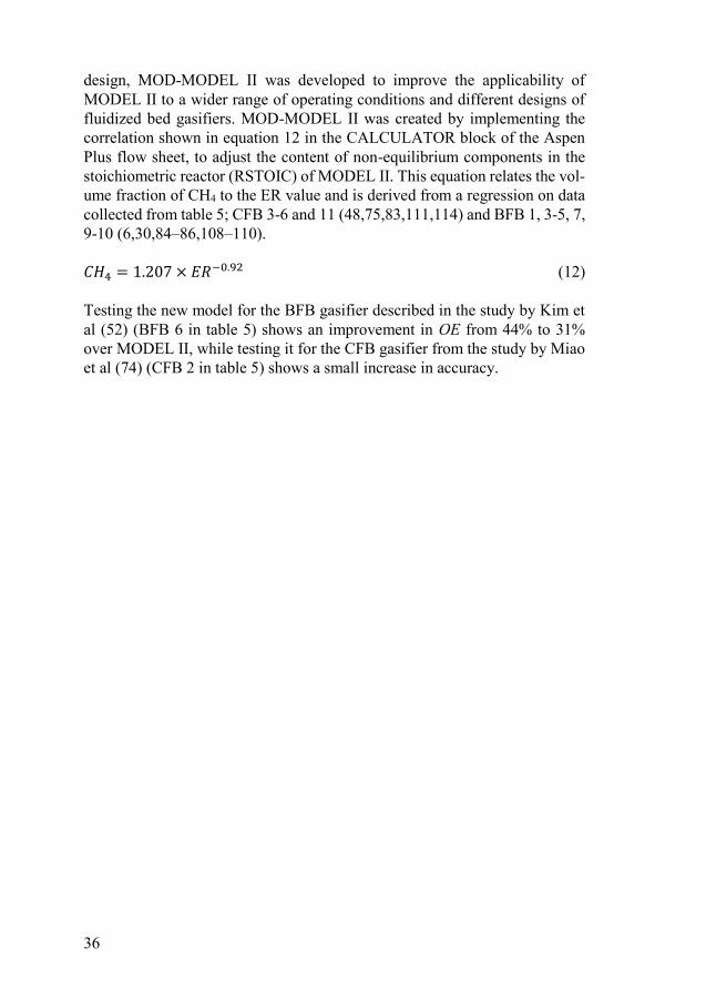
36

design, MOD-MODEL II was developed to improve the applicability of MODEL II to a wider range of operating conditions and different designs of fluidized bed gasifiers. MOD-MODEL II was created by implementing the correlation shown in equation 12 in the CALCULATOR block of the Aspen Plus flow sheet, to adjust the content of non-equilibrium components in the stoichiometric reactor (RSTOIC) of MODEL II. This equation relates the vol-ume fraction of CH4 to the ER value and is derived from a regression on data collected from table 5; CFB 3-6 and 11 (48,75,83,111,114) and BFB 1, 3-5, 7, 9-10 (6,30,84–86,108–110).

𝐶𝐶𝐶𝐶4 = 1.207 × 𝐸𝐸𝐸𝐸−0.92 (12)

Testing the new model for the BFB gasifier described in the study by Kim et al (52) (BFB 6 in table 5) shows an improvement in OE from 44% to 31% over MODEL II, while testing it for the CFB gasifier from the study by Miao et al (74) (CFB 2 in table 5) shows a small increase in accuracy.

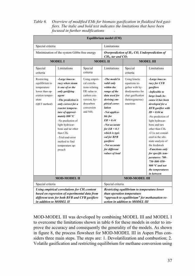
37

Table 6. Overview of modified EMs for biomass gasification in fluidized bed gasi-fiers. The italic and bold text indicates the limitations that have been focused in further modifications .

MOD-MODEL III was developed by combining MODEL III and MODEL I to overcome the limitations shown in table 6 for these models in order to im-prove the accuracy and consequently the generality of the models. As shown in figure 8, the process flowsheet for MOD-MODEL III in Aspen Plus con-siders three main steps. The steps are: 1. Devolatilization and combustion; 2. Volatile gasification and restricting equilibrium for methane conversion using

Equilibrium model (EM)

Special criteria Limitations

Minimization of the system Gibbs free energy Overprediction of H2, CO, Underprediction of CH4, tar and CO2

MODEL I MODEL II MODEL III

Special criteria

Limitations Special criteria

Limitations Special criteria

Limitations

Restricting equilibrium to temperature lower than op-eration temper-ature (QET method)

-Large inaccu-racy when steam is one of or the only gasifying agent -The prediction is only correct for a reactor tempera-ture of approxi-mately 800 °C -No prediction of light hydrocar-bons and tar other than CH4 -Trial-and-error method to find temperature ap-proach

Using empiri-cal correla-tions relating ER value to carbon con-version, hy-drocarbon conversion and NH3

-The model is valid only within the range of the data used for deriving em-pirical corre-lation -Not applica-ble for ER > 0.44 -Not accurate for ER < 0.3 which is typi-cal for BFB gasifiers -Not accurate for different values of load

Using kinetic equations to-gether with hy-drodynamics for char gasification (heterogeneous) reactions

-Large inaccu-racy for CFB gasifiers -Inflexible to large loads be-cause it has been developed for a BFB gasifier with ID = 0.04 m -No prediction of light hydrocar-bons and tars other than CH4 -Cl is not consid-ered in the ulti-mate analysis of the feedstock -Functions only for specific tem-peratures: 700–750–800–850–900 °C and not the temperatures in between

MOD-MODEL II MOD-MODEL III

Special criteria Special criteria Using empirical correlations for CH4 content based on regression of experimental data from different tests for both BFB and CFB gasifiers in addition to MODEL II

Restricting equilibrium to temperature lower than operation temperature “approach to equilibrium” for methanation re-action in addition to MODEL III

38

QET approach; and 3. Char gasification, which begins in the bed and contin-ues in the freeboard. The QET considered in RGIBBS for the second step is -350 °C. The negative value represents a QET which is lower than the assigned temperature to the RGIBBS.

Figure 8. MOD-MODEL III flow sheet in Aspen plus

When tested for a CFB gasifier described by Wu et al (83) (CFB 4 in table 5) and a BFB gasifier tested by Turn et al (84) (BFB 5 in table 5), MOD-MODEL III shows a large improvement in accuracy over MODEL I and MODEL III. The overall error is reduced from 50% to 40% for the CFB gasifier and from 36% to 8% for the BFB gasifier in comparison to MODEL III.

4.2.2.2 Kinetic-combined-hydrodynamic model

Paper IV examines another type of semi-empirical model for gasification in order to answer RQ1. This model is based on combination of a kinetic rate model and a hydrodynamic model. As explained in the methodology section (see 3.3) and presented in paper IV, different steps are coupled to develop a model for the gasification as shown in figure 9. The input parameters shared between three models are biomass characteristics (ultimate and proximate analysis), gasifier size (diameter and height), biomass and gasifying agent flow, superficial gas velocity, and reactor temperature. Each of the models also requires specific additional input data as shown in figure 9.

FEED

STEAM

AIR

GAS

SOLID

SEP

Devolatilization and combustion stage

Volatile gasification and restricting methane formation

Char gasification in bed and freeboard

FEED

STEAM

5

AIR

GAS

SOLID

SEP

Devolatilization and combustion stage

Volatile gasification and restricting methane formation

Char gasification in bed and freeboard

FEED

STEAM

AIR

GAS

SOLID

SEP

Devolatilization and combustion stage

Volatile gasification and restricting methane formation

Char gasification in bed and freeboard

FEED

STEAM

5

AIR

GAS

SOLID

SEP

Devolatilization and combustion stage

Volatile gasification and restricting methane formation

Char gasification in bed and freeboard

39

Figure 9. Overview on development of kinetic-hydrodynamic models in this thesis

Table 7 shows an overview of the results from the three models in predicting volume fraction of H2, CO, CO2 and CH4 for the bubbling fluidized beds pre-sented in papers by Radmanesh et al (30), Bilodeau et al (23), Narvaez et al (6), and Arena et al (86). These gasifiers are BFB 4, 8, 1 and 7 from table 5. The performance of the models in predicting gas and tar yield for BFB 8, 1 and 7, since the experimental data for these parameters are available has also been compared. The green color highlights the best accuracy in predicting the respective component.

In the case of BFB 4 (30), the overall accuracy of the KIN model is higher than that of the other models. This is especially when predicting the CH4 con-tent in the product gas. For BFB 8 (23), the overall performance of all models is within an acceptable range (error less than 30%). In this case the accuracy of KIN is improved by including the hydrodynamic model. However, TPT shows even better performance and lower error in predicting gas composition than CCBM. TPT mainly shows improvement in the accuracy of predicting H2 content compared to KIN in this gasifier. In the case of BFB 1 (6), although the average error level in predicting the content of CO, CO2 and CH4 is less than 30 %, the general performance of the models is not acceptable. Specially this can be seen for H2 content where the error is greater than 50 % with all three models. Overall, TPT performed better than the other models, and CCBM also improved the accuracy of the KIN model. The three models did not perform acceptably in predicting H2 and CH4 content in BFB 7 (86), but were sufficiently accurate in predicting CO and CO2 content. As in other cases, TPT was also more accurate than the other models in this case.

Generally, TPT shows better accuracy compared to the other models for all cases. This suggests that including simple hydrodynamics improves the per-formance of a kinetic-only model. Also it can be concluded that TPT model is not only the most accurate model in predicting gas composition but also the most general model compared to KIN and CCBM.

The results in table 7 also demonstrate that the models provide an accepta-ble overall accuracy for gas yield, although tar yield is not well predicted in

Ultimate and proximate analysis ofthe feedstockBiomass flow (kg/s)Air flow (m3/s)S/B ratio (-)Particle size (m)

Bed diameter (dBed, m)

Bed height (hBed, m)

Bed temperature (Tb, K)

Freeboard diameter (dFrb, m)

Freeboard height (hFrb, m)

Freeborad temperature (Tf, K)

Superficial velocity (u0, m/s)

Devolatilization sub-model Kinetic sub-model

Residence time (t, s)No hydrodynamic

model

Minimum fluidization velocity (umf, m/s)Voidage at umf (ɛmf ,-)

Two phase structure

Minimum fluidization velocity (umf, m/s)Voidage at umf (ɛmf ,-)

Bed height at umf (hmf, m)Descending emulsion phase (Xemd, (-))

Two phase structureand Counter current

back mixing

TPT

Hydrodynamic sub-model

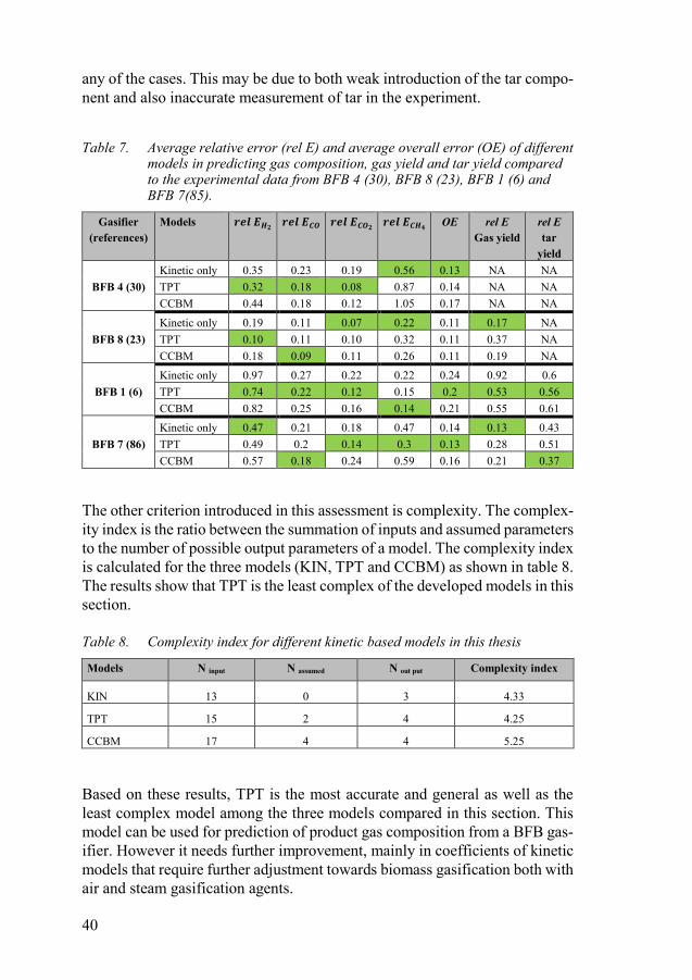
40

any of the cases. This may be due to both weak introduction of the tar compo-nent and also inaccurate measurement of tar in the experiment.

Table 7. Average relative error (rel E) and average overall error (OE) of different models in predicting gas composition, gas yield and tar yield compared to the experimental data from BFB 4 (30), BFB 8 (23), BFB 1 (6) and BFB 7(85).

Gasifier (references)

Models 𝒓𝒓𝒓𝒓𝒓𝒓 𝑬𝑬𝑯𝑯𝟐𝟐 𝒓𝒓𝒓𝒓𝒓𝒓 𝑬𝑬𝑪𝑪𝑪𝑪 𝒓𝒓𝒓𝒓𝒓𝒓 𝑬𝑬𝑪𝑪𝑪𝑪𝟐𝟐 𝒓𝒓𝒓𝒓𝒓𝒓 𝑬𝑬𝑪𝑪𝑯𝑯𝟒𝟒 OE rel E Gas yield

rel E tar

yield

BFB 4 (30) Kinetic only 0.35 0.23 0.19 0.56 0.13 NA NA TPT 0.32 0.18 0.08 0.87 0.14 NA NA CCBM 0.44 0.18 0.12 1.05 0.17 NA NA

BFB 8 (23) Kinetic only 0.19 0.11 0.07 0.22 0.11 0.17 NA TPT 0.10 0.11 0.10 0.32 0.11 0.37 NA CCBM 0.18 0.09 0.11 0.26 0.11 0.19 NA

BFB 1 (6) Kinetic only 0.97 0.27 0.22 0.22 0.24 0.92 0.6 TPT 0.74 0.22 0.12 0.15 0.2 0.53 0.56 CCBM 0.82 0.25 0.16 0.14 0.21 0.55 0.61

BFB 7 (86) Kinetic only 0.47 0.21 0.18 0.47 0.14 0.13 0.43 TPT 0.49 0.2 0.14 0.3 0.13 0.28 0.51 CCBM 0.57 0.18 0.24 0.59 0.16 0.21 0.37

The other criterion introduced in this assessment is complexity. The complex-ity index is the ratio between the summation of inputs and assumed parameters to the number of possible output parameters of a model. The complexity index is calculated for the three models (KIN, TPT and CCBM) as shown in table 8. The results show that TPT is the least complex of the developed models in this section.

Table 8. Complexity index for different kinetic based models in this thesis

Models N input N assumed N out put Complexity index

KIN 13 0 3 4.33

TPT 15 2 4 4.25

CCBM 17 4 4 5.25

Based on these results, TPT is the most accurate and general as well as the least complex model among the three models compared in this section. This model can be used for prediction of product gas composition from a BFB gas-ifier. However it needs further improvement, mainly in coefficients of kinetic models that require further adjustment towards biomass gasification both with air and steam gasification agents.

41

4.2.3 Empirical model (Statistical model) Paper V demonstrates the use of statistical methods to develop an empirical model as a route towards a general model for biomass gasification. As ex-plained in section 3.4, the empirical models are based on the linear regression equations derived by the PLS-R method (as shown in equation 3) on the da-taset formed by the data from CFB 1-8 and 10 from table 5. The coefficients (b1 to bn in equation 3) and the Y intercept (b0) for the model are presented in table 9. It should be noted that the sign of the coefficients in table 9 indicate whether they influence the results positively or negatively. This model is used to calculate the volume fraction of components in product gas (CH4, H2, CO, CO2, C2H4) from biomass gasification via CFB gasifiers. The model can also predict carbon conversion, dry gas yield, tar yield and lower heating value of the product gas.

42

Although the PLS-R model was already cross validated within the dataset, it had to be validated further in order to be used for predictions at other operating

Table 9. Regression coefficients forming the PLS model for each component in the pro-duct gas, heating value, carbon conversion, dry gas yield and tar yield based on equation 3.

Volume fraction a

CH4 (%)

Volume fraction

H2 (%)

Volume fraction

CO (%)

Volume fraction

CO2 (% )

Volume fraction

C2H4 (%)

LHV gas

(MJ/m3)

Carbon

conversion Dry gas

yield (m3/kg)

Tar yield (g/nm3)

Y intercept (the same unit as each output

parameter)

19.5861 -0.5385 65.1464 12.2715 7.9233 5.4012 4.8839 1.3001 10.6190

Temperature (°C)

-0.0110 0.0505 -0.0251 -0.0134 -0.0003 0.0009 0.0765 0.0005 -0.0208

Pressure (atm) 0.3544 0.2128 2.3013 -2.7144 -0.1305 0.2703 1.7230 -0.1142 0.3174

ER value -14.2789 -7.4821 -28.3998 49.1981 -1.4746 -5.6307 26.5232 5.0774 -11.9813

Bed volume (m3)

0.0090 -0.0656 0.2099 -0.1874 0.0252 0.0372 0.1920 -0.0051 -0.0584

Load b (kg/m2.h)

-0.0003 -0.0007 0.0007 0.0004 -0.0002 0.0000 0.0019 -0.0001 0.0002

B/V c (kg/m3.h)

-0.0010 -0.0031 0.0013 0.0037 -0.0011 -0.0003 0.0076 -0.0004 0.0016

Silica sand 0.2551 -0.7256 1.4744 -0.9785 -0.0590 0.3128 -0.2395 -0.0907 0.3657

Dolomite -0.2077 -1.0950 -1.9243 3.4192 -0.3413 -0.4264 0.1179 0.2681 -0.3480

Olivine -0.1981 2.7206 -0.2180 -2.5965 0.5440 -0.0231 0.2846 -0.1782 -0.2197

Particle size (mm)

-0.1417 -0.1689 -0.2986 0.5797 -0.0117 -0.0451 0.6417 0.0358 -0.2147

Mass fraction of ash (%)

0.0001 0.0430 -0.0736 0.0538 0.0030 -0.0294 -0.1618 -0.0263 0.1012

Mass fraction of moisture

(%)

-0.2134 -0.1149 -0.0025 0.2968 0.0179 -0.0348 0.9939 -0.0163 -0.0941

Mass fraction of C (%)

-0.0500 -0.0463 -0.1866 0.3200 -0.0375 -0.0596 -0.1459 0.0101 0.1285

Mass fraction of H (%)

-0.4186 0.1658 -0.1594 0.6005 -0.1646 -0.1195 -0.0953 0.2218 -0.1918

C/Hd 0.2737 -0.9398 -0.9913 1.5908 -0.0203 -0.2343 -0.4044 -0.2704 1.1434

Mass fraction of O (%)

0.1934 -0.1494 0.0716 -0.1677 -0.0313 0.1400 0.0344 0.0049 -0.0847

S/Be -0.0452 -0.2156 -4.2611 3.2971 0.8026 -0.4141 -3.4195 0.4504 -1.3277

HHV Biomass (MJ/kg)

0.0202 0.0892 0.2276 -0.2703 -0.0478 -0.0108 0.0824 -0.0133 0.1689

a. All the volume fractions are dry basis b. Load= Biomass flow (kg/h)/reactor cross sectional area (m2) c. B/V= Biomass flow (kg/h)/reactor volume (m3) d. C/H= Carbon content in biomass/all hydrogen in biomass included moisture content and steam content e. S/B= steam flow(kg/h)/Biomass flow(kg/h)

43

conditions. This validation was performed on 15 independent data points (meaning points that were not used to create the PLS model) which are listed in table 10. Since paper V studies CFB gasifiers, all the points used for vali-dation of the model are taken from CFB gasifiers.

Table 10. Data points used for validation of the PLS model

Table 11 shows that most of the components in the product gas are predicted well by the empirical model. R2 is above 0.5 and the Ave. E is less than 40% for all of the components in the product gas. However, the model does not predict values for tar yield accurately, not only due to an insufficient number of data points but also as a result of discrepancies in defining tar components in experiments. Dry gas yield, carbon conversion and heating value of the product gas are predicted with acceptable accuracy (Ave. E< 0.15).

Table 11. R2, RMSEP and average error (Ave E) for validation of the PLS model based on data in table 9

Gasifiers ERa Temperature (◦C)

Bed material S/Bb Bed volume (m3)

Ref

ECN 0.38 843 Silica sand 0 0.1884 (75) ECN 0.34 855 Silica sand 0 0.1884 (75) TPS 0.2 897 Dolomite 0 0.9812 (112) TPS 0.19 850 Dolomite 0 0.9812 (112) Li 0.37 772 Silica sand 0.0039 0.0510 (48) Li 0.37 789 Silica sand 0 0.0510 (48) Wu 0.19 690 Silica sand 0 0.628 (83) VTT 0.31 885 Dolomite 0.1314 0.206 (44) VTT 0.39 900 Dolomite 0.1682 0.206 (44) Miao 0.27 775 Silica sand 0 24.76 (74) Miao 0.27 765 Silica sand 0 24.76 (74) Chris 0.3 750 Silica sand 0 0.0286 (77) Chris 0.3 800 Olivine 0 0.0286 (77) Meng 0.38 780 Silica sand 0.93 0.0297 (50) Meng 0.39 820 Silica sand 0.9 0.0297 (50) a. Equivalence ratio is an index for the ratio input air (oxygen) mass to the stoichiometric air (oxygen) needed for full combustion b. Steam flow(kg/h)/Biomass flow(kg/h)

Predicted parame-ter

Volume

fraction

CH4 (%)

Volume

fraction

H2 (% )

Volume

fraction

CO (%)

Volume

fraction

CO2 (%)

Volume

fraction

C2H4

(%)

LHV (MJ/m3)

Carbon conver-

sion

Dry gas yield

(m3/kg)

Tar yield

(g/nm3)

R2 0.7 0.8 0.53 0.6 0.83 0.82 0.5 0.6 0.26

RMSEP 1.39 2.41 3.98 3.14 0.53 0.51 6.72 0.25 1.7

Ave. E 0.15 0.13 0.13 0.08 0.36 0.11 0.08 0.11 0.45

44

4.3 The key operating parameters influencing the bio-mass gasification in fluidized beds

In order to identify the parameters with the most significant impact and ad-dress RQ2, the interrelation between different input parameters and output must be determined. Using PCA and PLS-R on the wide range of dataset provides the necessary platform. The results in this section are adapted from paper V and are presented in figure 10 and table 12. Figure 10 shows the re-sults from PCA analysis while table 12 presents the p-values derived from the PLS-R model. The green color in the table represents the input parame-ters that influence the respective output parameters positively while red color represents the input parameters with negative impact on the respective out-put parameters.

Based on the results in figure 10 and table 12, the most effective parameter is ER value, followed by bed materials. Other parameters that show significant effects on product gas quality are particle size, temperature, C content, olivine, pressure, load, moisture content, H and O content, steam to biomass ratio, bed volume and higher heating value of the biomass.

45

Figure 10. Loadings plots which show the correlation existing between different pa-rameters. The arrows indicate input and output parameters with negative correlation, while the small dashed circles indicate input and output pa-rameters with positive correlation.

Table 12 shows that the input parameters temperature, ER value, moisture content of biomass and particle size have a positive influence on carbon con-version. Therefore, improving carbon conversion requires increasing the value of these parameters, however, doing so can have a negative impact on gas quality and gasifier performance.

Since ER value is directly related to the oxygen/air content in the system, it can shift the gasification system towards combustion when it is increased. Higher ER value thus leads to reformation of lighter H-C components and consequently decrease of product gas heating value. Basically, increasing ER value results in more conversion of H-Cs to CO and CO2 and therefore a de-crease in tar yield and CH4 content in the product gas. The more H-C conver-sion there is the more gas is produced. ER increase also results in temperature

Carbonconversion

CO2 (vol%)

Dolomite

Particle size(mm)

Silica sand

Cold gas efficiency

Tar yield(g/nm3)

Olivine

Ash (wt%)

Moisture (wt%)

H (wt%)

HHV Biomass(MJ/kg)

C (wt%)

C/HTemperature (°C)

Pressure(atm)

CO (vol%)

CH4(vol%)

LVH gas (MJ/m3)

C2H4(vol%)

O (wt%)

B/V (kg/m3 h)

Load (kg/m2 h) Dry gas yield(m3/kg)

ER Value

H2 (vol%)S/B

Silica sand

CO (vol%)

Load (kg/m2 h)

H (wt%)

C (wt%)

C2H4 (vol%)

ER Value

CO2(vol%)

DolomiteC/H

Carbonconversion

Cold gas efficiency

O (wt%)

H2 (vol%)S/B

Olivine

Pressure(atm)

Particle size(mm)

HHV Biomass(MJ/kg)

Dry gas yield(m3/kg)

B/V (kg/m3 h)

Reactorvolume (m3)

CH4 (vol%)

Ash (wt%)Moisture

(wt%)

LVH gas (MJ/m3)

Tar yield(g/nm3)

HHV Biomass(MJ/kg)

C (wt%)

H (wt%)

Dry gas yield(m3/kg)

ER Value

S/B

CO2 (vol%)

Olivine

B/V (kg/m3 h)

Load (kg/m2 h)H2 (vol%)

Temperature (°C)

Pressure (atm)

LVH gas (MJ/m3)

CH4 (vol%)O (wt%)

Cold gas efficiency

Silica sand

CO (vol%)

Ash (wt%)

Moisture(wt%)

C2H4(vol%)

Dolomite

Tar yield(g/nm3)

C/H

Particle size (mm)

Reactorvolume (m3)

Carbonconversion

Reactorvolume (m3)

Temperature (°C)

46

increase if the system is operated autothermally. If the gasifier is operated al-lothermally, increasing the external heat will result in temperature increase and consequently enhance the water gas shift (WGS) reaction (see subsection 2.2) towards producing more CO. This means that temperature has both posi-tive and negative impacts on CO content in the product gas depending on the heating system of the gasifier and also the specific reaction that dominates the process. Temperature increase due to enhanced steam gasification of char and methane reforming reactions (see 2.2) towards more H2 production also in-creases hydrogen content in product gas.

The other operating parameter which is important for steam gasification of biomass is S/B ratio (see 3.1). Based on figure 10 and table 12, the S/B ratio has a positive impact on light H-Cs and C2H4 content and a negative impact on CO content in the product gas. Increasing the steam rate and consequently S/B ratio shifts the WGS reaction towards conversion of CO and production of H2 in the product gas. This impact is anticipated mostly for auto-thermal gasification without any external heating source.

Biomass characteristics influence the product gas quality in different ways. Ultimate analysis of the biomass (C, H and O) affects heating value of the product gas. Biomass with higher oxygen content, which consequently results in higher volatile material content, produces higher CH4 and other light H-C contents in the product gas. This is due to release of more volatile material in the devolatilization step which remains unconverted through the process. These components (CH4 and light H-Cs) contribute considerably to the heat-ing value of the product gas, so higher O content (while H and C content are low) increases the heating value of the product gas.

In case of proximate analysis of the biomass, specifically moisture content, there is a significant negative impact on CH4 content and a positive impact on carbon conversion. If the biomass has a high moisture level, part of the heat available in the gasifier will be used to evaporate non-bound water, and con-sequently the remaining heat will not be sufficient to devolatilize biomass en-tirely to volatile components such as CH4 and light H-Cs. Moreover, based on the methane reforming reaction (see 2.2), lower water content in the system would lead to more unconverted CH4. However, increasing water content in the system generally enhances gasification reactions towards increased con-version of carbon to other components. This occurs mainly due to the water gas shift (WGS) reaction and the other steam reforming reactions shown in table 2 (see 2.2).

Biomass particle size is another characteristic of feedstock which correlates positively with CH4 content and tar yield and negatively with carbon conver-sion and CO2 content in the product gas. Since smaller particles have more surface area, in the devolatilization step carbon is more converted to light H-Cs which are less prone to further conversion in the gasification step. On the other hand, biomass with smaller particle size results in more unconverted tar

47

and less gas. In general, tar yield varies with temperature as an operating pa-rameter and particle size as a biomass characterization. To decrease tar content in the product gas, these parameters should be increased.

Another operating parameter that impacts gas quality in fluidized bed gas-ifiers is bed material. There is a positive correlation between presence of oli-vine, H2 content and light H-Cs in the product gas. This is due to enhancement of tar reforming reactions through the catalytic effect of olivine. Increased carbon conversion using dolomite as the bed material is also based on in-creased tar conversion. In the case of dolomite, the WGS reaction also shifts toward increased consumption of H2 and CO, while using olivine increases H2 and C2H4 production and decreases CO2 production. Generally, more gas is produced when using in-bed catalysts such as dolomite and olivine.

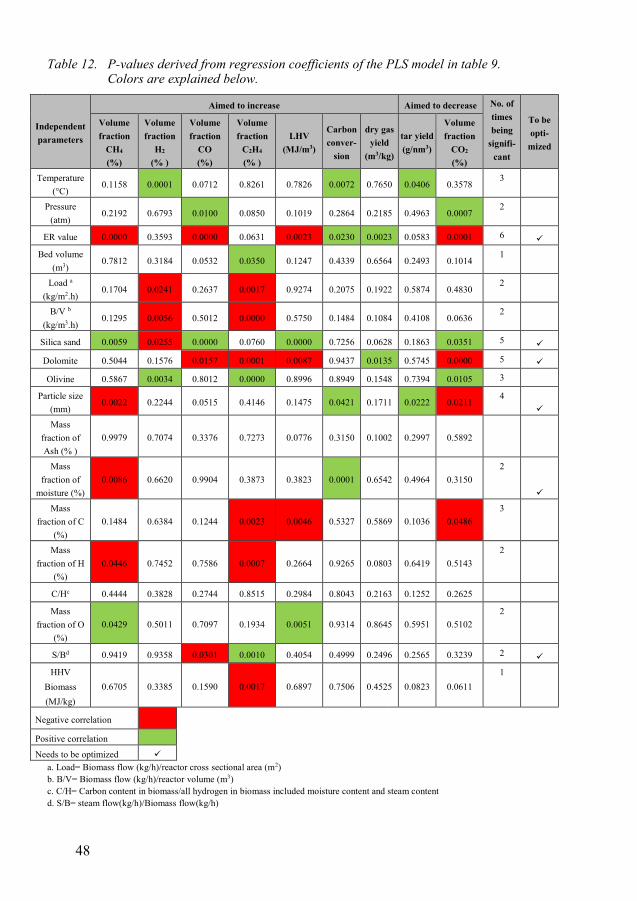
48

Table 12. P-values derived from regression coefficients of the PLS model in table 9. Colors are explained below.

Independent parameters

Aimed to increase Aimed to decrease No. of times being

signifi-cant

To be opti-

mized

Volume fraction

CH4 (%)

Volume fraction

H2 (% )

Volume fraction

CO (%)

Volume fraction

C2H4 (% )

LHV (MJ/m3)

Carbon conver-

sion

dry gas yield

(m3/kg)

tar yield (g/nm3)

Volume fraction

CO2 (%)

Temperature (°C)

0.1158 0.0001 0.0712 0.8261 0.7826 0.0072 0.7650 0.0406 0.3578 3

Pressure (atm)

0.2192 0.6793 0.0100 0.0850 0.1019 0.2864 0.2185 0.4963 0.0007 2

ER value 0.0000 0.3593 0.0000 0.0631 0.0023 0.0230 0.0023 0.0583 0.0001 6

Bed volume (m3)

0.7812 0.3184 0.0532 0.0350 0.1247 0.4339 0.6564 0.2493 0.1014 1

Load a (kg/m2.h)

0.1704 0.0241 0.2637 0.0017 0.9274 0.2075 0.1922 0.5874 0.4830 2

B/V b

(kg/m3.h) 0.1295 0.0056 0.5012 0.0000 0.5750 0.1484 0.1084 0.4108 0.0636

2

Silica sand 0.0059 0.0255 0.0000 0.0760 0.0000 0.7256 0.0628 0.1863 0.0351 5

Dolomite 0.5044 0.1576 0.0157 0.0001 0.0087 0.9437 0.0135 0.5745 0.0000 5

Olivine 0.5867 0.0034 0.8012 0.0000 0.8996 0.8949 0.1548 0.7394 0.0105 3

Particle size (mm)

0.0022 0.2244 0.0515 0.4146 0.1475 0.0421 0.1711 0.0222 0.0211 4

Mass fraction of Ash (% )

0.9979 0.7074 0.3376 0.7273 0.0776 0.3150 0.1002 0.2997 0.5892

Mass

fraction of moisture (%)

0.0086 0.6620 0.9904 0.3873 0.3823 0.0001 0.6542 0.4964 0.3150 2

Mass fraction of C

(%) 0.1484 0.6384 0.1244 0.0023 0.0046 0.5327 0.5869 0.1036 0.0486

3

Mass

fraction of H (%)

0.0446 0.7452 0.7586 0.0007 0.2664 0.9265 0.0803 0.6419 0.5143 2

C/Hc 0.4444 0.3828 0.2744 0.8515 0.2984 0.8043 0.2163 0.1252 0.2625

Mass fraction of O

(%) 0.0429 0.5011 0.7097 0.1934 0.0051 0.9314 0.8645 0.5951 0.5102

2

S/Bd 0.9419 0.9358 0.0301 0.0010 0.4054 0.4999 0.2496 0.2565 0.3239 2 HHV

Biomass (MJ/kg)

0.6705 0.3385 0.1590 0.0017 0.6897 0.7506 0.4525 0.0823 0.0611 1

Negative correlation

Positive correlation

Needs to be optimized a. Load= Biomass flow (kg/h)/reactor cross sectional area (m2)

b. B/V= Biomass flow (kg/h)/reactor volume (m3) c. C/H= Carbon content in biomass/all hydrogen in biomass included moisture content and steam content d. S/B= steam flow(kg/h)/Biomass flow(kg/h)

49

Biomass gasification in the fluidized bed gasifier can also be optimized based on the knowledge gained about the interrelated operating parameters and the correlations existing between input parameters and gas quality. The empirical model developed using the PLS-R method (see 4.2.3) can be used as the basis for determining the optimal operating condition for the fluidized bed gasifier (specially CFB gasifier). As explained in the methodology (see 3.4), optimi-zation is performed using the genetic algorithm (GA) in Matlab, where deci-sion variables (see 3.4) are selected by identifying the parameters with the opposite impact on product gas and gasifier performance. This has been done based on the information in table 12. Through the optimization process, all parameters other than decision variables are fixed on the average value in the data set for that parameter while the decision variables are only varying within the range that is defined for them as presented in section 3.4.

In this thesis three cases have been considered as the aim of optimization. In each case three scenarios are created for three different bed materials: silica sand scenario; dolomite scenario; and olivine scenario. The aims of the cases are briefly described as follows:

1. Best gas composition case. This case is aimed at maximizing CH4, H2, CO and C2H4 content and minimizing CO2 content, as well as ob-taining the highest possible heating value of the product gas. The case is identified to investigate the optimized trade-off between operating parameters for high quality gas when tar yield, carbon conversion and dry gas yield are not the focus.

2. Least tar yield, most dry gas yield and carbon conversion case. Highest carbon conversion and dry gas yield, measured as the volume (m3) of dry gas produced for each kilogram of dry biomass gasified, are the aim of this case. Tar yield also needs to be minimized. This case is identified to show the other extreme focus in gasification that is to have high dry gas yield, high carbon conversion and low tar yield while gas quality is not of concern. This results in high CO2 content and low H2, CO and CH4 content. It is important to highlight that in this condition although the produced gas content and carbon conversion are high, the quality of the gas produced is not high.

3. All dependent parameters case. All dependent parameters are aimed at producing high quality product gas along with a high level of heating value, carbon conversion and dry gas yield. Low level of tar yield is also an aim in this case. This case is identified to show the trade-off between operating parameters when all the criteria evaluating gasi-fiers performance are considered.

50

As shown in table 13, the best gas composition case is achieved in the olivine scenario by setting ER value at 0.17 with biomass moisture content of 3.5% and an average particle size smaller than 1mm (0.10 mm to be precise). Tar yield, however, is relatively high compared to other cases where carbon con-version and gas yield are relatively low. It can be concluded that in order to produce gas with high LHV and maximum CH4, H2, CO and C2H4 content with minimum CO2 content, the ER value should be in the lower bound (ER<0.3). The biomass needs to have moisture content around 4% and particle size < 1 mm. These ranges only apply if olivine is used as the bed material.

The second case is also achieved in the olivine scenario, with ER value in the upper bound (0.6), S/B ratio 0.37 and biomass with 7% moisture and av-erage particle size close to 5mm. In this case the recommended ranges for operating the gasifier are ER > 0.4 and S/B > 0.3 and less than 1. For the aim of this case biomass should have moisture content around 10% and particle size around 4 mm.

Finally, olivine is also recommended for the third case as in the other cases. In this case the ER value should be equal to 0.26 and S/B ratio to 0.39 while biomass should have average particle size of 6 mm and moisture content of 13%. Accordingly the ideal range of operation conditions when olivine is used

Table 13. Selected and representative results of optimization

Bed material scenarios

Optimized values for the components Optimum operating points

Volume fraction

of CH4 (%)

Volume fraction

of H2

(% )

Volume fraction

of CO (%)

Volume fraction

of CO2 (%)

Volume fraction

of C2H4 (%)

LHV (MJ/m3)

Carbon convers-

ion

Dry gas yield

(m3/kg)

Tar yield

(gr/nm3)

ER Particle size

(mm)

Mass frac-tion of

Moisture content

(%)

S/B Best scenar-

ios

Best gas composition case

Silica sand 12.76 20.60 37.41 28.60 1.35 5.80 75.22 1.52 7.81 0.20 0.27 3.54 0.09

Dolomite 11.30 19.49 30.56 38.07 0.99 4.25 78.93 2.13 6.02 0.17 0.88 7.31 0.23

Olivine 12.31 27.77 35.31 23.48 2.52 5.34 75.64 1.15 7.16 0.17 0.10 3.50 0.00

Least tar yield, most dry gas yield and carbon conversion case

Silica sand 4.52 15.70 21.06 57.37 0.55 2.64 93.06 4.32 0.33 0.71 6.37 4.03 0.11

Dolomite 4.63 15.88 17.27 61.28 0.20 1.63 91.62 4.52 0.33 0.64 2.24 6.43 0.14

Olivine 4.64 23.26 20.00 49.86 2.18 2.40 92.42 3.63 0.15 0.61 4.42 7.14 0.37

All dependent parameters case Silica sand 8.58 17.93 30.84 40.74 1.80 4.46 88.30 2.28 4.06 0.30 3.82 13.65 0.68

Dolomite 8.48 17.48 22.78 49.77 1.12 2.99 84.15 3.28 2.57 0.32 5.43 7.36 0.73

Olivine 8.17 24.96 29.38 35.31 2.81 4.09 89.79 1.83 3.45 0.26 5.74 13.02 0.39

51

as bed material is the average value for the input parameters (ER ≈ 0.3, S/B ≈ 0.7, moisture content ≈ 9% and particle size ≈ 3mm).

52

5 Conclusion

One of the major challenges in this field is to model the main unit operation in the gasification process, the gasifier, as generally as possible. Based on the efforts described in this thesis to address two research questions; first to assess the approaches for developing a general model and second to determine the parameters with the most significant impact on the product gas quality and gasifier performance, the following points can be concluded.

Development of a general and accurate model for biomass gasification Developing a general model for biomass gasification in fluidized bed gasifiers is possible by considering different aspects:

Using an equilibrium model (EM) reduces the amount of data required, and therefore increases the generality potential of the model but has low accuracy for predicting product gas composition especially regarding CO and CH4 content.

The accuracy of the EM can be improved by considering quasi-equilib-rium temperature (QET) for some of the non-equilibrium reactions. How-ever, determination of this temperature is based on a trial-and-error ap-proach which reduces the generality of the model.

Modification of the EM using empirical correlations improves accuracy, although the model is only accurate and applicable within the range of input parameters used to develop the model. Therefore, including more empirical data from wider range of variation is needed to overcome this limitation.

Improving the accuracy of the EM by including kinetic and hydrodynamic equations for char gasification works well, but it is limited to the specific type, geometry and design of gasifier. Therefore the generality of this model is relatively low.

Considering quasi-equilibrium temperature for the methane formation re-action and including char gasification reaction kinetics in the EM over-come the limitations of either approach and enhance their generality.

Although models based on reaction kinetics and hydrodynamic equations also require data on geometry and size of the gasifier, their generality can still be improved. Testing these models on different gasifiers shows that including hydrodynamic equations improves the accuracy of kinetic-only models.

53

A two phase structure model, based on the idea of not only dividing the reactor to bubble and emulsion phases, but also considering that reactions occur in both phases, is used as a hydrodynamic sub-model for modeling bubbling fluidized bed gasifiers. Compared to other hydrodynamic mod-els studied in this thesis, this model shows more generality, less complex-ity and better accuracy when combined with a kinetic-only model.

Assessment of the empirical model developed by partial least square (PLS) approach shows that if the gasifier is operated within the range of input parameters used for developing the model, the accuracy of the model will be high.

The most effective operating conditions on the product gas composition Investigating the data collected from different types of gasifiers shows

that the fluidized bed gasifier is the best choice for producing bio-methane through gasification.

Based on the multivariate analysis of the dataset used for developing the empirical model, equivalence ratio (ER) is the parameter with the most significant impact on gasifier performance and product gas quality.

Optimizing the operation of FBs based on this model shows that high gas quality (high H2, CO and CH4 content and low CO2 content), high carbon conversion and low tar yield is achieved at ER ≈ 0.3, S/B ≈ 0.7, moisture content ≈ 9% and particle size ≈ 3mm, with olivine as the bed material. This optimum was determined over a range of conditions with varying ER (0.17-0.73), S/B ratio (0-1.45), moisture content (3.5-22%), and particle size (0.1-10.25 mm). Silica sand, dolomite and olivine were different op-tions for the bed material.

54

6 Future work

Based on the findings presented in this thesis, there is still room for further improvement of the fluidized bed gasification models, mainly in relation to tar yield prediction. This may be achieved by including more experimental data in empirical models and developing new reaction kinetic models for tar for-mation. Improving detection and analysis of more tar species from an experi-mental point of view would assist the accuracy of models. However, the mod-els developed in this thesis are useful at the current level of accuracy for sys-tem-level analysis, system integration, economic analysis and process optimi-zation. Implementing the kinetic-combined-hydrodynamic models developed in this thesis, to the Aspen Plus for analysis of large scale plants for producing biofuel, chemicals, heat and power is another potential area of future studies. This would enhance the connection between the gasifier block and other op-eration blocks in process simulation for different purposes such as power pro-duction or chemical product processes.

Models developed in this thesis can also be used for design and operation of lab and pilot-scale gasifiers. Therefore, another area for future work will be to build a lab or pilot-scale gasifier and use the knowledge gained from the models in this thesis to operate and investigate the impact of different operat-ing parameters on the gasifier performance and quality of the gas, empirically.

55

References

1. IEA Sankey diagram [Internet]. [cited 2016 Jul 31]. Available from: http://www.iea.org/Sankey/index.html#?c=World&s=Final consumption

2. Demirel Y. Energy and energy types. In: Production, Conversion, Storage, Conservation, and Coupling. Springer-Verlag London; 2012. p. 27–70.

3. Hackl R, Arvidsson M, Lundin B, Harvey S. Process integration study of a biorefinery producing ethylene from lignocellulosic feedstock for a chemical cluster. In: 6th Dubrovnik Conference on Sustainable Development of Energy, Water and Environment Systems. Dubrovnik; 2011.

4. Higman, Christopher; van der Burgt M. Gasification. 2nd ed. Gulf professional Publishing; 2008.

5. Gomez Barea A, Leckner B. Modeling of biomass gasification in fluidized bed. Prog Energy Combust Sci. 2010;36:444–509.

6. Narvaez I, Orio A, Aznar MP, Corella J. Biomass gasification with air in an atmospheric bubbling fluidized bed . Effect of six operational variables on the quality of the produced raw gas. Ind Eng Chem Res. 1996;5885(95):2110–20.

7. Kopyscinski J, Schildhauer TJ, Biollaz SMA. Production of synthetic natural gas ( SNG ) from coal and dry biomass – A technology review from 1950 to 2009. Fuel. Elsevier Ltd; 2010;89(8):1763–83.

8. Lunde P, Kesler FL. Carbon dioxide methanation on a ruthenium catalyst. Ind Eng Chem Process Des Dev. 1974;13(1):27–33.

9. Mirmoshtaghi G, Westermark M, Mohseni F. Simulation of lab-scale methantion reactor. In: International conference of applied energy. 2012. p. 1–10.

56

10. Yoshida H, Kiyono F, Tajima H, Yamasaki A. Two-stage equilibrium model for a coal gasifier to predict the accurate carbon conversion in hydrogen production. Fuel. 2008;87:2186–93.

11. Yan H, Heidenreich C, Zhang D. Mathematical modelling of a bubbling fluidised-bed coal gasifier and the significance of “ net flow.” Fuel. 1998;77(9):1067–79.

12. Wang Y, Kinoshita CM. Kinetic model of biomass gasification. Sol Energy. 1993;51(1):19–25.

13. Sharma AK. Equilibrium and kinetic modeling of char reduction reactions in a downdraft biomass gasifier : A comparison. Sol Energy. 2008;82:918–28.

14. Knoef H. Handbook Biomass Gasification. 2nd ed. Biomass Technology group (btg); 2012.

15. Warnecke R. Gasification of biomass : comparison of fixed bed and fluidized bed gasifier. Biomass and Bioenergy. 2000;18:489–97.

16. Olofsson I, Nordin A, Söderlind U. Initial review and evaluation of process technologies and systems suitable for cost-efficient medium-scale gasification for biomass to liquid fuels. 2005.

17. Review of Technologies for Gasification of Biomass and Wastes Final report. 2009.

18. Kwant KW, Knoef H. Status of gasification in countries participating in the IEA biomass gasification and GasNet activity September 2002. 2002.

19. Basu P. Combustion and gasification in fluidized beds. Taylor and Francis group; 2006.

20. Upadhye AA, Qi W, Huber GW. Conceptual process design: A systematic method to evaluate and develop renewable energy technologies. AIChE J. 2011;57(9):2292–301.

21. Beheshti SM, Ghassemi H. Process simulation of biomass gasification in a bubbling fluidized bed reactor. Energy Convers Manag. Elsevier Ltd;

57

2015;94:345–52.

22. Ghassemi H, Shahsavan-markadeh R. Effects of various operational parameters on biomass gasification process ; a modified equilibrium model. Energy Convers Manag. Elsevier Ltd; 2014;79:18–24.

23. Bilodeau JF, Therien N, Proulx P, Czernik S, Chimique DDG. A mathematical model of fluidized bed biomass gasification. Can J Chem Eng. 1993;71:549–57.

24. Alimuddin Z, Zainal B, Lahijani P, Mohammadi M, Rahman A. Gasification of lignocellulosic biomass in fluidized beds for renewable energy development : A review. Renew Sustain Energy Rev. Elsevier Ltd; 2010;14(9):2852–62.

25. Ab WAW, Ghani K, Moghadam RA, Salleh MAM, Alias AB. Air gasification of agricultural waste in a fluidized bed gasifier: hydrogen production performance. Energies. 2009;2:258–68.

26. Rapagna S, Jand N, Kiennemann A, Foscolo PU. Steam-gasification of biomass in a fluidised-bed of olivine particles. Biomass and Bioenergy. 2000;19:187–97.

27. Mansaray KG, Ghaly AE, Al-taweel AM, Hamdullahpur F. Air gasification of rice husk in a dual distributor type fluidized bed gasifier. Biomass and Bioenergy. 1999;17:315–32.

28. Tasaka K, Furusawa T, Tsutsumi A. Biomass gasification in fluidized bed reactor with Co catalyst. Chem Eng Sci. 2007;62:5558–63.

29. Puig-arnavat M, Bruno JC, Coronas A. Review and analysis of biomass gasification models. Renew Sustain energy Rev. 2010;14(9):2841–51.

30. Radmanesh R, Chaouki J, Guy C, Hc Q. Biomass gasification in a bubbling fluidized bed reactor : Experiments and modeling. AIChE J. 2006;52(12):4258–72.

31. Buragohain B, Mahanta P, Moholkar VS. Thermodynamic optimization of biomass gasification for decentralized power generation and Fischer-Tropsch synthesis. Energy. Elsevier; 2010;35(6):2557–79.

58

32. Li XT, Grace JR, Watkinson AP, Lim CJ, Ergurdenler A. Equilibrium modeling of gasification: a free energy minimization approach and its application to a circulating fluidized bed coal gasifier. Fuel. 2001;80:195–207.

33. Sadaka SS, Ghaly AE, Sabbah MA. Two-phase biomass air-steam gasiÿcation model for uidized bed reactors : Part III — model validation. Biomass and Bioenergy. 2002;22:479–87.

34. Gururajan V, Agarwal P, Agnew J. Mathematical modeling of fluidized bed coal gasifiers. Trans IChemE. 1992;70a:211–38.

35. Zainal ZA, Ali R, Lean CH, Seetharamu KN. Prediction of performance of a downdraft gasifier using equilibrium modeling for different biomass materials. Energy Convers Manag. 2001;42:1499–515.

36. Jand N, Brandani V, Foscolo PU. Thermodynamic limits and actual product yields and compositions in biomass gasification processes. Ind Eng Chem Res. 2006;45:834–43.

37. D. Bacon, J. Downie, J. Hsu and J. Peters, Eds., D. Bacon, J. Downie JH and JP. Modeling of fluidized bed gasifiers. In: Overend RP, K. TM, L.K.Mudge, editors. Fundamentals of thermochemical biomass conversion. London: Elsevier Applied Science; 1985. p. 717–32.

38. Sotudeh-Gharebaagh R, Legros R, Chaouki J, Paris J. Simulation of circulating fluidized bed reactors using Aspen plus. Fuel. 1998;77(4):327–37.

39. Gururajan V, Agarwal P, Agnew J. Mathematical modeling of fluidized bed coal gasifiers. Trans IChemE. 1992;70a:211–38.

40. Zainal ZA, Rifau A, Quadir GA, Seetharamu KN. Experimental investigation of a downdraft biomass gasifier. Biomass and Bioenergy. 2002;23:283–9.

41. Lim Y, Lee U. Quasi-equilibrium thermodynamic model with empirical equations for air – steam biomass gasi fi cation in fl uidized-beds. Fuel Process Technol. Elsevier B.V.; 2014;128:199–210.

42. Kersten SRA, van der Drift A, Prins W, van Swaaij WPM. Interpretation of

59

Biomass Gasification by “Quasi”-Equilibrium Models. In: 12th, European biomass conference; biomass for energy, industry and climate protection. Amsterdam; 2002.

43. Doherty W, Reynolds A, Kennedy D. The effect of air preheating in a biomass CFB gasifier using Aspen Plus simulation. Biomass and Bioenergy. Elsevier Ltd; 2009;33(9):1158–67.

44. Hannula I, Kurkela E. A semi-empirical model for pressurised air-blown fluidized-bed gasification of biomass. Bioresour Technol. Elsevier Ltd; 2010;101(12):4608–15.

45. Nikoo MB, Mahinpey N. Simulation of biomass gasification in fluidized bed reactor using Aspen plus. Biomass and Bioenergy. 2008;32(12):1245–54.

46. Schläpfer P, Tobler J. Theoretische und praktische untersuchungen uber den betrieb von motorfahrzeugen mit holzgas. schweizerische gesellschaft fur das stadium der motorbrenstoff. Bern: Selbstverl. d. Gesellschaft; 1937.

47. Gumz W. Gas producers and blast furnaces. New York: John Wiley & Sons, Inc.; 1950.

48. Li XT. Biomass gasification in a circulating fluidized bed. University of British Columbia; 2002.

49. Li XT, Grace JR, Lim CJ, Watkinson AP, Chen HP, Kim JR. Biomass gasification in a circulating fluidized bed. Biomass and Bioenergy. 2004;26(2):171–93.

50. Meng X, de Jong W, Fu N, Verkooijen AHM. Biomass gasification in a 100 kWth steam-oxygen blown circulating fluidized bed gasifier: Effects of operational conditions on product gas distribution and tar formation. Biomass and Bioenergy. Elsevier Ltd; 2011;35(7):2910–24.

51. Campoy M, Gómez-barea A, Vidal FB, Ollero P. Air – steam gasification of biomass in a fluidised bed : Process optimisation by enriched air. Fuel Process Technol. Elsevier B.V.; 2009;90(5):677–85.

52. Doo Kim Y, Won Yang C, Jong Kim B, Su Kim K, Woo Lee J, Hong Moon J, et al. Air-blown gasification of woody biomass in a bubbling fluidized bed gasifier. Appl Energy. Elsevier Ltd; 2013;112:414–20.

60

53. Fiaschi D, Michelini M. A two-phase one-dimensional biomass gasification kinetics model. Biomass and Bioenergy. 2001;21:121–32.

54. Andersson D, Karlsson M. Invesitigation of the effects of introducing hydrodynamic parameters into a kinetic biomass gasification model for a bubbling fluidized bed. Vasteras; 2014.

55. Asadi-saghandi H, Sheikhi A, Sotudeh-gharebagh R. Sequence-based process modeling of fluidized bed biomass gasification. Sustain Chem Eng. 2015;3:2640–51.

56. Rafati M, Hashemisohi A, Wang L, Shahbazi A. Sequential modular simulation of hydrodynamics and reaction kinetics in a biomass bubbling fluidized-bed gasifier using Aspen plus. Energy and Fuels. 2015;29(12):8261–72.

57. Blasi C Di, Buonanno F, Branca C. Reactivities of some biomass chars in air. Carbon N Y. 1999;37:1227–38.

58. Fryer C, Potter OE. Countercurrent backmixing model for fluidized bed catalytic reactors. Applicability of simplified solutions. Ind Eng Chem Eundam. 1972;11(3):338–44.

59. Kunni D, Octave L. Flow modeling of fast fluidized beds. In: Circulating fluidized bed technology III. 1990. p. 91–8.

60. Kato K, Wen CY. Bubble assemblage model for fluidized bed catalytic reactors. Chem Eng Sci. 1969;24:1351–69.

61. Toomey RD, Johnstone HF. Gaseous fluidization of solid particles. Chem Eng Prog. 1952;48:220–5.

62. Kunni D, Levenspiel O. Fluidization engineering. 2nd ed. Butterworth-Heinemann; 1991.

63. Mostoufi N, Cui H, Chaouki J. A comparison of two- and single-phase models for fluidized-bed reactors. Ind Eng Chem Res. 2001;40:5526–32.

64. Yang W-C. Handbook of fluidization and fluid-particle systems. Pittsburg:

61

Marcel Dekker inc.; 2003.

65. Van Deemter JJ. Mixing and contacting in gas-solid fluidized beds. Chem Eng Sci. 1961;13:143–54.

66. Dellavedova M, Derudi M, Biesuz R, Lunghi A, Rota R. On the gasification of biomass : Data analysis. Process Saf Environ Prot. Institution of Chemical Engineers; 2011;90(3):246–54.

67. Guo B, Li D, Cheng C, Zi-an L, Shen Y. Simulation of biomass gasification with a hybrid neural network model. Bioresour Technol. 2001;76:77–83.

68. Esbensen KH, Guyot D, Westad F, Houmoller LP. Multivariate data analysis-in practice: an introduction to multivariate data analysis and experimental design. CAMO ASA; 2002.

69. Multivariate Analysis [MVA] - Types of Methods [Internet]. CAMO. [cited 2016 Oct 13]. Available from: http://www.camo.com/resources/multivariate-types-methods.html

70. Manuel J, Cristoforetti G, Legnaioli S, Lorenzetti G, Palleschi V, Shaltout AA. Classical univariate calibration and partial least squares for quantitative analysis of brass samples by laser-induced breakdown spectroscopy. Spectrochim Acta Part B At Spectrosc. Elsevier B.V.; 2010;65(8):658–63.

71. Darwish HW, Backeit AH. Multivariate versus classical univariate calibration methods for spectrofluorimetric data : Application to simultaneous determination of olmesartan medoxamil and amlodipine besylate in their combined dosage form. J Fluoresc. 2013;23:79–91.

72. Loha C, Chatterjee PK, Chattopadhyay H. Performance of fluidized bed steam gasification of biomass – Modeling and experiment. Energy Convers Manag. Elsevier Ltd; 2011;52(3):1583–8.

73. Alipour R, Yusup S, Azlina W, Nehzati S, Tavasoli A. Investigation on syngas production via biomass conversion through the integration of pyrolysis and air – steam gasification processes. Energy Convers Manag. Elsevier Ltd; 2014;87:670–5.

74. Miao Q, Zhu J, Barghi S, Wu C, Yin X, Zhou Z. Model validation of a CFB biomass gasification model. Renew Energy. 2014;63:317–23.

62

75. Van Der Drift a., Van Doorn J, Vermeulen JW. Ten residual biomass fuels for circulating fluidized-bed gasification. Biomass and Bioenergy. 2001;20(1):45–56.

76. Lv P, Yuan Z, Ma L, Wu C, Chen Y, Zhu J. Hydrogen-rich gas production from biomass air and oxygen / steam gasification in a downdraft gasifier. Renew Energy. 2007;32:2173–85.

77. Christodoulou C, Grimekis D, Panopoulos KD, Vamvuka D, Karellas S, Kakaras E. Circulating fluidized bed gasification tests of seed cakes residues after oil extraction and comparison with wood. Fuel. Elsevier Ltd; 2014;132:71–81.

78. E. Kurkela PS and JL. Pressurized fluidized bed gasification experiments with wood, peat, and coal at VTT 1: Test facilities and gasification experiments with sawdust," VTT. Espo,, Finland;

79. Guo XJ, Xiao B, Zhang XL, Luo SY, He MY. Experimental study on air-stream gasification of biomass micron fuel ( BMF ) in a cyclone gasifier. Bioresour Technol. Elsevier Ltd; 2009;100(2):1003–6.

80. Gallier PW, Evans LB, Britt HI, Boston JF, Gupta PK. Aspen:Advanced capabilities for modeling and simulation of industrial processes. In: Computer applications to chemical engineering. p. 293–308.

81. He J. Gasification-based biorefinery for mechanical pulp mills. [Sundsvall]: Mittuniversitetet; 2014.

82. Dahlquist E, Jone A. Presentation of a dry black liquor gasification process with direct causticization. Tappi J. 2005;4(5):15–9.

83. Jianzhi W, Bingyan X, Zhenfang L, Xiguang Z. Performance analysis of a biomass circulating fluidized bed gasifier. Biomass and Bioenergy. 1992;3(2):105–10.

84. Turn S, Kinoshita C, Ishimura D. An experimental investigation of Hydrogen production. Int J Hydrogen Energy. 1998;23(8):641–8.

85. Lv PM, Xiong ZH, Chang J, Wu CZ, Chen Y, Zhu JX. An experimental

63

study on biomass air – steam gasification in a fluidized bed. Bioresour Technol. 2004;95:95–101.

86. Arena U, Zaccariello L, Mastellone ML. Gasification of natural and Waste biomass in a pilot scale fluidized bed reactor. Combust Sci Technol. 2010;182:625–39.

87. Nunn TR, Howard JB, Longwell JP, Peters WA. Product compositions and kinetics in rapid pyrolysis of sweet gum wood. Ind Eng Chem Process Des Dev. 1985;24:836–44.

88. Biggs MJ, Agarwaf PK. The CO / CO2 product ratio for a porous char particle within an incipiently fluidized bed : a numerical study. Chem Eng Sci. 1997;52(6):941–52.

89. Mohlen HJ, Sulimma A. High temperature, high pressure thermogravimetry of coal gasification-apparatus, data acuisition and numerical evaluation. Thermochim Acta. 1986;103:163–8.

90. Westbrook CK, Dryer L. Chemical kinetic modeling of hydrocarbon combustion. Prog Energy Combust Sci. 1984;10:1–57.

91. Macak J, Malecha J. Mathematical model for the gasification of coal under pressure. Ind Eng Chem Process Des Dev. 1978;17(1):92–8.

92. Gerun L, Paraschiv M. Numerical investigation of the partial oxidation in a two-stage downdraft gasifier. Fuel. 2008;87:1383–93.

93. Dryer FL. High temperature oxidation of carbon monoxide and methane in a turbulant flow reactor. 1972.

94. Gerber S, Behrendt F, Oevermann M. An Eulerian modeling approach of wood gasification in a bubbling fluidized bed reactor using char as bed material. Fuel. Elsevier Ltd; 2010;89(10):2903–17.

95. Smoot LD, Smith PJ. Coal combustion and gasification. Plenum Chemical Engineering Series. Newyork: Plenum press; 1985.

96. Jess A. Mechanisms and kinetics of thermal reactions of aromatic hydrocarbons from pyrolysis of solid fuels. Fuel. 1996;75(12):1441–8.

64

97. Morf P, Hasler P, Nussbaumer T. Mechanisms and kinetics of homogeneous secondary reactions of tar from continuous pyrolysis of wood chips. Fuel. 2002;81(7):843–53.

98. Ching-yen S, Lin C. An improved bubble assemblage model for fluidized-bed catalytic reactors. Chem Eng Sci. 1993;48(7):1299–308.

99. Hoffman A, Janssen P. Particle segregation in fluidized binary mixtures. Chem Eng Sci. 1993;48:1583–92.

100. The Unscrambler Methods. CAMO Software AS; 2006.

101. Westad F, Martens H. Variable selection in near infrared spectroscopy based on significance testing in partial least squares regression. J near infrared Spectrosc. 2000;124:117–24.

102. D. Kalyanmoy. Multi-objective optimization using evolutionary algorithms. John Wiley & Sons, Inc.; 2001.

103. Holland J. Adaptation in natural and artificial systems. Cambridge, MA: MIT Press; 1992.

104. Esfahani IJ, Yoo C. An optimization algorithm-based pinch analysis and GA for an off-grid batteryless photovoltaic-powered reverse osmosis desalination system. Renew Energy. 2016;91:233–48.

105. Campana PE, Li H, Zhang J, Zhang R, Liu J, Yan J. Economic optimization of photovoltaic water pumping systems for irrigation. Energy Convers Manag. 2015;95:32–41.

106. Shengwei Wang XX. Parameter estimation of internal thermal mass of building dynamic models using genetic algorithm. Energy Convers Manag. 2006;47:1927–41.

107. Jong W De, Unal O, Andries J, Hein KRG, Spliethoff H. Biomass and fossil fuel conversion by pressurised fluidised bed gasification using hot gas ceramic filters as gas cleaning. Biomass and Bioenergy. 2003;25:59–83.

108. Skoulou V, Koufodimos G, Samaras Z, Zabaniotou A. Low temperature

65

gasification of olive kernels in a 5-kW fluidized bed reactor for H2-rich producer gas. Int J Hydrogen Energy. Elsevier Ltd; 2008;33(22):6515–24.

109. Subramanian P, Sampathrajan A, Venkatachalam P. Fluidized bed gasification of select granular biomaterials. Bioresour Technol. Elsevier Ltd; 2011;102(2):1914–20.

110. Wan WA, Karim Ghani A, Alipour Moghadam R, Mohd Salleh MA, Alias AB. Air gasification of agricultural waste in a fluidized bed gasifier: Hydrogen production performance. Energies. 2009;2:258–68.

111. García-Ibañez P, Cabanillas A, Sánchez JM. Gasification of leached orujillo (olive oil waste) in a pilot plant circulating fluidised bed reactor. Preliminary results. Biomass and Bioenergy. 2004;27(2):183–94.

112. Waldheim, Lars; Fredriksson C. Evaluation of the pilot plant test on cane trash. 2002.

113. Kurkela, E.; Stahlberg, P.; Laatikainen J. Pressurized fluidized bed gasification experiments with wood, peat, and coal at VTT[ Espo, Finland] in 1991-1992. 1: Test facilities and gasification experiments with sawdust. Espo; 1993.

114. Sheeba KN, Chandra JS, Jaisankar S. Air gasification characteristics of coir pith in a circulating fluidized bed gasifier. Energy Sustain Dev. 2009;13:166–73.

115. Barrio M. Experimental investigation of small-scale gasification of woody biomass. The Norwegian university of science and technology; 2002.

116. Dogru M, Howarth CR, Akay G, Keskinler B, Malik AA. Gasification of hazelnut shells in a downdraft gasifier. Energy. 2002;27:415–27.

117. Zhou J, Chen Q, Zhao H, Cao X, Mei Q, Luo Z, et al. Biomass – oxygen gasification in a high-temperature entrained- flow gasifier. Biotechnol Adv. 2009;27:606–11.

118. Zhao Y, Sun S, Tian H, Qian J, Su F, Ling F. Characteristics of rice husk gasification in an entrained flow reactor. Bioresour Technol. Elsevier Ltd; 2009;100(23):6040–4.

66

119. Kobayashi N, Tanaka M, Piao G, Kobayashi J, Hatano S, Itaya Y. High temperature air-blown woody biomass gasification model for the estimation of an entrained down-flow gasifier. Waste Manag. Elsevier Ltd; 2009;29(1):245–51.