biomonitoring guide - west african survey training workshop 2009...
TRANSCRIPT
Survey Training Workshop Ivory Coast, February/March 2009 GRASP/ MPI/ WCF
1
Biomonitoring Guide – Survey Training Workshop Taï National Park, Côte d’Ivoire, February/March 2009
JUNKER Jessica (Max Planck Institute for Evolutionary Anthropology, Leipzig, Germany) N’GORAN K. Paul (Centre Suisse de Recherches Scientifiques en Côte-d’Ivoire / Wild Chimpanzee Foundation)
KOUAKOU Y. Célestin (Centre Suisse de Recherches Scientifiques en Côte-d’Ivoire / Wild Chimpanzee Foundation)
KÜHL Hjalmar (Max Planck Institute for Evolutionary Anthropology, Leipzig, Germany)
© Damien Caillaud

Survey Training Workshop Ivory Coast, February/March 2009 GRASP/ MPI/ WCF
2
Acknowledgements I would like to thank the following people for their input and support: Paul N’Goran,
Célestin Yao Kouakou, Dr. Hjalmar Kuehl, Dr. Serge Wich, Dr. David Jay, Dr. Ilka
Herbinger, Dr. Jessica Ganas, Prof. Christophe Boesch, Dr. Linda Vigilant, Dr. Fabian
Fabian Leendertz, Claudia Nebel, Christina Kompo, Geneviève Campbell, and all the other
people who made this workshop possible.

Survey Training Workshop Ivory Coast, February/March 2009 GRASP/ MPI/ WCF
3
Table of Contents 1. GENERAL INTRODUCTION...................................................................................................................4
2. AN INTRODUCTION TO SAMPLING AND DATA ANALYSIS.........................................................5
2.1 RANDOM ERROR AND SYSTEMATIC ERROR ...............................................................................................6 2.2 ACCURACY AND PRECISION......................................................................................................................6 2.3 RANDOM VS. SYSTEMATIC SAMPLING ......................................................................................................6 2.4 STRATIFICATION ......................................................................................................................................7 2.5 ASSUMPTIONS ..........................................................................................................................................7 2.6 FREQUENCY DISTRIBUTIONS ....................................................................................................................8 2.7 IMPORTANCE OF SAMPLE SIZE ..................................................................................................................9 2.8 BASIC STATISTICS ....................................................................................................................................9 2.9 DIFFERENT MEASURES OF PRECISION .....................................................................................................10 2.10 STATISTICAL TESTS AND HYPOTHESIS TESTING ....................................................................................10
3. INTRODUCTION TO DISTANCE SAMPLING...................................................................................11
3.1 ASSUMPTIONS FOR ESTIMATING THE NUMBER OF OBJECTS DETECTED IN ‘COVERED’ AREA (NA)............15 3.2 CONVERTING NEST DENSITY INTO POPULATION DENSITY .......................................................................16 3.3 SURVEY DESIGN .....................................................................................................................................17 3.4 INTRODUCTION TO ANALYSIS IN DISTANCE 5.0 ......................................................................................20
4. INTRODUCTION TO TEMPORAL INFERENCES ............................................................................25
5. INTRODUCTION TO SPATIAL ANALYSES USING ARCVIEW-ARCMAP .................................27
6. SUMMARIZING AND PRESENTING SURVEY RESULTS...............................................................34
7. COLLECTION OF ORGANIC SAMPLES FOR DNA ANALYSIS....................................................37
8. A PAN-AFRICAN APE TREND ESTIMATION PROGRAM .............................................................38
9. THE IUCN/SSC/PSG/SGA A.P.E.S. DATABASE..................................................................................39
9.1 EDITING INFORMATION ON THE IUCN/SSC/PSG/SGA A.P.E.S. WEBSITE .............................................39
10. INFORMATION SOURCES ..................................................................................................................41
11. EXERCISES.............................................................................................................................................42
12. APPENDICES..........................................................................................................................................44

Survey Training Workshop Ivory Coast, February/March 2009 GRASP/ MPI/ WCF
4
1. General introduction
For more than 100 years, ecologists have estimated populations of animals to describe their
status and trends. Great apes were no exception and over the past 30 years considerable
effort and resources have been devoted to the monitoring of their populations to collect
information on abundance, rates of population change and factors influencing their
populations in different regions. Such information is key to informing and evaluating
management decisions to ensure their protection. Despite these efforts however, few
accurate and precise data are available to date that allow for reliable estimation of
abundance and population change. Reasons for the shortage of high quality survey
information are the lack of monitoring programs with a uniform and robust sampling
protocol and the difficult work and observation conditions in tropical forests, causing
research and monitoring to become relatively expensive and time-consuming.
Estimates of great ape population size and rates of population change over time
may vary in quality. Such estimates range from “educated guesses”, based on interviews
with local people living in or close to forests, to sample-based methods, which aim at
estimating a mean density over a large area by extrapolation, to long-term studies of
individual registrations. Although fairly accurate, the latter method is neither feasible nor
cost-effective and habituating and monitoring multiple groups of individuals over a large
area can take several years.
Since the 1980s, habitat fragmentation, hunting and illegal killing and disease have
resulted in precipitous declines of great ape populations throughout Africa. Consequently,
concerned scientists tried to estimate the size of entire populations and monitor changes in
their distribution and abundance. However, survey and monitoring efforts should also
collect information on factors that may positively influence their populations as well as all
major threats that jeopardize their long-term survival.
The most efficient survey method for large areas of tropical rain forest is using
line-transects. To date, most great ape surveys have been carried out using nest counts for a
specific site-based purpose. Great apes build nests that consist of vegetative structures that
can remain visible for weeks or months and sample-based methods generally involve
indirect counts of nests rather than direct counts of the apes themselves. Much effort has
therefore gone into estimating the size of ape populations by counting their nests which (i)
are much more numerous than their makers (ii) do not run away and (iii) are more visible.
Nests accumulate over many months in any given area. Counting nest density thus allows
us to estimate population density, assuming a standing crop of nests which decay at a given
rate at a given site at a given season. Therefore, they are less sensitive than direct
observations to short-term fluctuations in local density (due to seasonality).
A problem associated with this method is the conversion of nest counts into great
ape population estimates. A constant fixed relationship between nest density and ape
density does not exist. The rate of nest decay varies greatly between sites and seasons, so
ideally surveys should incorporate a locally-derived and seasonally-appropriate estimate of
nest decay rate. However, the data required to estimate nest decay can take more than a
year to collect prior to the actual survey. Another problem is accessibility and the size of
the areas that have to be covered on foot. All too often time and budget do not allow for
walking entire study areas and as a result, accuracy and precision of estimates may be
greatly lowered. Consequently, most surveys have been site-based and many large areas
Survey Training Workshop Ivory Coast, February/March 2009 GRASP/ MPI/ WCF
5
have been surveyed only once or not at all, due to lack of human and financial resources.
Furthermore, existing data are often not precise enough to detect meaningful shifts in
population size and many datasets, such as those recorded in unpublished reports, are not
accessible to the ape conservation community.
Thus, there is a clear need for a unified great ape monitoring program that yields
reliable and easily accessible results in a time-efficient manner and that addresses the
causes of ape population change at different sites and in different countries and regions
(for a summary of the proposed program see section 6). Such a program would combine
previous sampling locations, ongoing field projects and sites not previously surveyed to
obtain abundance and trend estimates and quantify their underlying causes.
This workshop is a first attempt to link and coordinate past, present and future
survey efforts by creating a network of conservation agencies, national environmental
government agencies and local communities involved in survey work in the different West
African great ape range countries. With this workshop we also hope to ensure high data
quality levels and the rapid processing of the data collected in the field, as well as to
contribute to capacity building in the region.
2. An introduction to sampling and data analysis
While it is easy to ask questions such as “How many chimpanzees are there in Sapo
National Park?” or “How often do chimpanzees build nests?” in most cases, exact answers
to these questions cannot be known. Instead the answers are estimated, using sampling
methods. For instance, one could count the number of chimpanzees that exist in only a part
of Sapo National Park, using a predetermined sampling methodology, or one could observe
a limited number of chimpanzees for a predetermined period of time and count note how
often these individuals build nests. If this methodology is well designed then the number of
chimpanzees counted in only a portion of the park will provide a relatively accurate (see
below) estimate of the number of chimpanzees that live in the entire park; the mean
number of nests built by a fraction of the total number of chimpanzees will provide a
relatively accurate estimate of how often chimpanzees build nests in general.
When using line transect methods, the location of transects should be representative
of the larger sampling area or population. If the transects that are sampled are
“representative”, then they will contain the same number of animals in the same proportion
(or density) as the entire sampling area. If knowledge of the area and population is limited
however, it may be difficult to be sure that transects are representative of the entire
sampling area. If this is the case, the most important aspect of sampling is to avoid
introducing any bias because of the way one samples.
For instance, if one were to survey the chimpanzee population in Taï National Park
and decide to sample close to roads because roads serve as easy access points to the forest,
then samples will not be representative of the area as a whole. This is because hunting
pressure and habitat alteration by humans are likely to be centred along roads, causing
chimpanzee densities to be lower there. Thus, the population estimate will be biased
because it will underestimate the true density of chimpanzees in the sampling area.

Survey Training Workshop Ivory Coast, February/March 2009 GRASP/ MPI/ WCF
6
2.1 Random error and systematic error
Random error refers to the variability in the results of a study and affects the precision, but
not the accuracy of an estimate, because if the error is truly random, there should be an
equal number of incorrect values both above and below the true value. Systematic error
(the influence of this error on the result is referred to as bias) describes a systematic or
consistent increase or decrease in results. For instance, if a chimpanzee population estimate
is constantly too low because surveys are conducted alongside roads, then the result is said
to have a negative bias and vice versa. A systematic error will affect the accuracy of a
result, but it will not necessarily affect its precision.
2.2 Accuracy and precision
Accuracy measures the closeness of the computed value to the true value, i.e. how close
the population estimate is to true population size. Accuracy of a survey result can only be
measured if true population size is known. Precision is the closeness of repeated measures
to one another and is especially important when estimating changes in population size (or
density) over time. Estimates can be accurate and precise (Fig. 1a), accurate but not precise
(Fig 1b), precise but not accurate (Fig 1c) or neither accurate nor precise (Fig 1d). During
sampling, the aim is to produce results that are both accurate and precise.
2.3 Random vs. systematic sampling
Random sampling refers to the method of choosing transect locations based on the
principle that if each part of an area or each entity has an equal chance of being sampled it
is unlikely that any systematic bias will affect the sample and it should therefore be
a b c d
Fig 1 Targets indicate level of accuracy and precision. Estimates (red crosses) may be
a) accurate and precise, b) accurate but not precise, c) precise but not accurate, or d)
neither accurate nor precise.

Survey Training Workshop Ivory Coast, February/March 2009 GRASP/ MPI/ WCF
7
representative of the entire sampling area or unit. Systematic sampling on the other hand
refers to the method of choosing transect locations based on the principle that regular
patterns rarely occur in nature. Here, transects are evenly distributed and regularly spaced.
This design has the advantage that it is generally easier to locate transects that are evenly
distributed through space than to locate random locations. Generally, good coverage of the
area (whether using random or systematic sampling) increases estimate precision.
2.4 Stratification
Sampling may be stratified (i.e. dividing the sampling area into distinct categories or
strata) when the estimate of population size is likely to be affected by some environmental
or human factor. In this case, obtaining separate estimates for each stratum will increase
precision of the overall population estimate for the entire sampling area. For instance, if
one was planning a chimpanzee survey in some conservation area with primary, secondary
and swamp forest, one would stratify by forest type as chimpanzee densities are likely to
differ among these habitats. Density estimates within each stratum should cluster closer
around their respective stratum means than around the overall mean density estimate for
the entire sampling area. Furthermore, in some cases it may be important to obtain habitat-
specific density estimates (e.g. to inform specific conservation management decisions).
Generally, the following factors should be considered when stratifying the sampling area:
major habitat types (that are likely to influence animal density/ distribution and seasonal
movements); human settlements; roads; extractive activities (e.g. mining, trading and
logging) and other centers of human activity.
2.5 Assumptions
All methods of data collection and analysis are based on certain assumptions that are
considered true. For example, when using line transect nest count methods, it is assumed
that all nests directly on the line are observed and counted and that less nests are observed
and counted further away from the line. When using strip transect methods on the other
hand, the assumption is that all objects within the boundaries of the strip transect (within a
certain width and length) are observed and counted, that no objects outside the strip
transect are counted and that no object is counted twice. To ensure that the assumptions are
met, observers need to give careful attention to details during the sampling process.
However, in some cases one cannot be sure that all assumptions are true (e.g. that each
object within the strip transect is observed and counted when these objects are animals that
move away fast when encountered). Different sampling and analysis methods are based on
different assumptions. When choosing the appropriate method to use it is important to
choose a method for which the underlying assumptions are most likely to be met. This of
course is case and site-specific.

Survey Training Workshop Ivory Coast, February/March 2009 GRASP/ MPI/ WCF
8
2.6 Frequency distributions
When using line transect sampling methods, the measurements collected will be ordinal
level measurements. These are ranked measurements (e.g. different age classes, different
distance classes etc.) and can be graphically presented as a range of values that have
different frequencies. This is referred to as the frequency distribution of the data collected.
The frequency distribution of a dataset includes a lot of information. For example, through
careful examination of a frequency distribution, one can make important conclusions
regarding the dataset, e.g. whether sample size was sufficient (Fig. 2a), observers correctly
rounded perpendicular distance values (Fig 2b), transects were placed correctly (i.e. were
representative, Fig. 2c) and about trends in frequencies over time Fig. 2d-e).
Frequency distributions can be symmetrical or asymmetrical. When the occurrence of each
sampling event is independent of prior occurrences within the sampling unit (i.e.
measurements are not influenced by one another) then the data are expected to follow the
shape of a normal distribution (also referred to as a parametric distribution) (Fig. 3a). The
normal distribution is always symmetrical around the mean value. If data that are expected
to follow a normal distribution (such as weight of male adult chimpanzees in Taï National
Park or daily distances traveled by hunters around Budongo Forest), but instead is distorted
0 5 10 15 20 25 30 35 400
5
10
15
20
Distance classes
Fre
quen
cy
0 5 10 15 20 25 30 35 400
5
10
15
20
Distance classes
Fre
quen
cy
0 5 10 15 20 25 30 35 400
5
10
15
20
Distance classes
Fre
quen
cy
0 5 10 15 20 25 30 35 400
5
10
15
20
Distance classes
Fre
qu
ency
0 5 10 15 20 25 30 35 400
5
10
15
20
Distance classes
Fre
qu
ency
a b c
d e
Fig. 2 Information contained in frequency distributions of sampling datasets may
reveal that a) sample size was not sufficient, b) observers incorrectly rounded
perpendicular distances to zero, transects were not placed in a representative way (e.g.
along roads where animals moved away from the approaching observer) and d-e) that
animal density has decreased over time (e.g. where the same transects were surveyed
twice at different points in time)

Survey Training Workshop Ivory Coast, February/March 2009 GRASP/ MPI/ WCF
9
in some way, this may provide interesting information for the manager/ researcher (e.g.
dominant male chimpanzees are significantly heavier than non-dominant males or hunters
travel much further on a daily basis than 10 years ago, suggesting that animal densities
have decreased near roads and other centers of human activity). Other frequency
distributions commonly discussed in the biological context are the Poisson (Fig. 3b), the
bimodal (Fig. 3c) or the binomial distribution.
Fig.
2.7 Importance of sample size
The sample size is the number of transects sampled. In other words, if one observes 300
chimpanzee nests on 50 line transects then the sample size is 50. Sample size is important
for the precision of the estimate: the larger the sample size, the higher the precision (an
increase in sample size decreases variance between line transects). While it is desirable to
sample as many line transects as possible, this is often not feasible logistically and
financially. Thus, it is important to find some balance between precision and the amount of
time, money and personnel available.
2.8 Basic statistics
Mean, median, mode and range are basic statistics that describe the distribution of the data
in a dataset. The mean (also referred to as the arithmetic mean or average) is the most
commonly used statistic and is calculated by adding all data points in a sample and
dividing it by the total number of data points (sample size). The median divides the
distribution into two equal halves – it is the value with an equal number of data points on
either side of it and is used to describe frequencies that are not normally distributed. The
mode is the value at the peak of the distribution (there may be more than one mode e.g.
when the distribution is bi- or multimodal). The range refers to the maximum spread of the
data and is represented by the minimum and maximum value in the dataset.
1 2 3 4 5 6 7 8 9 100
2
4
6
Value
Fre
quen
cy
1 2 3 4 5 6 7 8 9 100
3
6
9
12
Value
Fre
quen
cy
1 2 3 4 5 6 7 8 9 100
3
6
9
12
Value
Fre
quen
cy
a b c
Fig. 3 Illustration of a a) normal, b) Poisson and c) bimodal frequency distribution
Survey Training Workshop Ivory Coast, February/March 2009 GRASP/ MPI/ WCF
10
2.9 Different measures of precision
Precision can be measured in different ways. It may be expressed as Standard Deviation
(SD), Coefficient of Variation (CV), Standard Error of the Sample Mean (SEM, or short
Standard Error (SE)) or Confidence Limits (CL’s). The SD is calculated directly from all
observations of a particular variable and represents essentially the average of the deviation
from the mean. For normally distributed data, SD can be calculated by taking the square
root of the variance (where variance equals the square of the SD). The CV shows the SD as
a percentage of the mean. This single number indicates how widely (poor precision) or
narrowly (good precision) the values are clustered about the mean, irrespective of whether
the mean is small or large). Standard Error is the standard deviation divided by the square
root of the sample size. Confidence Limits are calculated values that fall above and below
the mean, where the biologically true value of the parameter estimated has a known
probability of falling within these bounds. This probability is called the confidence level
and is commonly set at 95%. In other words, if the same transect was sampled 100 times
then one would expect the calculated confidence limits to bracket the true mean 95 times.
The distance between the upper and the lower CL is the Confidence Interval (CI).
2.10 Statistical tests and hypothesis testing
Two or more datasets can be compared using different statistical tests. Which test to use
depends largely on the type of data collected (e.g. whether these are categorical, interval or
ordinal measurements) as well as the frequency distribution of the dataset (use either
parametric or non-parametric tests). Statistical tests provide the basis for deciding whether
two datasets are different merely due to chance events (due to random error) or whether
there are sufficient grounds to decide that they really are different.
For example, if one were to survey the same line transects in an area before and
after logging events, one would most probably find fewer nests after logging than before
logging, but in order to determine whether nest encounter rates differed during the course
of logging, one would need to analyse the two datasets by means of statistical testing. If
the results of the statistical analysis reveal that the two datasets are different, one also
refers to them as significantly different. Levels of significance (referred to as α-levels) are
routinely set at 0.05 (but may also be set at α = 0.01 or α = 0.001). In other words, if a
specific statistical test with α = 0.05 revealed a statistically significant difference between
chimpanzee nest encounter rates before and after logging, then there is a 95% chance that
chimpanzee nest encounter rates differed between periods of logging and no logging. Thus,
statistical tests cannot give an absolute answer to your question, but rather provide a
probability that two datasets differ (measured by comparing the means, medians or
variances of the two datasets). The ability of a statistical test to detect a difference
increases with increasing sample size, precision and effect size (i.e. the magnitude of the
difference to be detected).
The scientific method refers to gathering observable, empirical and measurable
data, and based on these, using statistical methods for investigating observed phenomena.
There is a standardized. Here, scientific researchers propose hypotheses as explanations of

Survey Training Workshop Ivory Coast, February/March 2009 GRASP/ MPI/ WCF
11
wL
n
A
ND
2
ˆˆ ==
awLP
n
A
ND
2
ˆˆ ==
phenomena, and design experimental studies to test these hypotheses. For example, if one
wanted to find out how logging affected stress levels in chimpanzees (e.g. measured by
Cortisol levels in their urine), one could collect urine samples of chimpanzees in a logging
concession before and after logging. One would (1) set up the null-hypothesis stating that
“there is no difference between Cortisol levels in the urine of chimpanzees before and after
logging” (the alternative hypothesis H1 would state that there is a difference). The next step
(2) would be to examine the frequency distributions of the two datasets and determine
whether these are distributed normally (this can be done with the aid of a statistical test).
Depending on the outcome of the normality test, (3) one would choose an appropriate
statistical test to assess the probability of randomly obtaining two means (or medians or
variances) as different as those obtained in the study. Last, if the statistical test reveals a
significant result (i.e. a difference between the two datasets) (4) reject the null hypothesis
and accept the alternative hypothesis or vice versa.
3. Introduction to distance sampling
In contrast to strip transect sampling where the observer travels down the centerline of a
long narrow strip counting all objects within the strip, line transect sampling entails
traveling along a line recording all detected objects as well as the perpendicular distance
from the line to each object detected. One major difference between these two methods is
that line transect sampling is not based on the critical assumption that all objects within a
specific area are detected, as is the case for strip transect sampling (i.e. based on the
assumption that all objects within the strip are detected). Here, it is important that all
objects on or near the line are detected, however, the method allows a proportion of objects
within a distance w (this distance varies according to visibility, vegetation density etc.) of
the line to be missed.
Distance sampling is an extension of strip transects sampling. In strip transect
sampling, we see everything in the covered region (or strip) and we can calculate animal/
nest density as, where N̂ is estimated population size, A is the size of
the
study region (total sampling area), n is the number of animals/ nests counted, w is the strip
half-width and L the total line length. In distance line transect sampling, we do not see
everything but only a proportion of animals/ nests within the covered region (denoted Pa)
and we estimate animal/ nest density as , where w is denoted
truncation distance (i.e. the furthest distance recorded). To estimate Pa, we need to measure
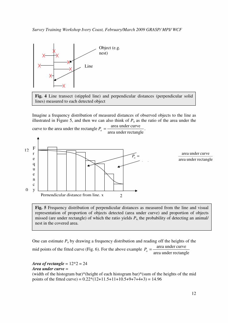
perpendicular distance from the transect line to each observed object (Fig 4).
Survey Training Workshop Ivory Coast, February/March 2009 GRASP/ MPI/ WCF
12
Imagine a frequency distribution of measured distances of observed objects to the line as
illustrated in Figure 5, and then we can also think of Pa as the ratio of the area under the
curve to the area under the rectanglerectangleunder area
curveunder area=aP .
One can estimate Pa by drawing a frequency distribution and reading off the heights of the
mid points of the fitted curve (Fig. 6). For the above example rectangleunder area
curveunder area=aP
Area of rectangle = 12*2 = 24
Area under curve =
(width of the histogram bar)*(height of each histogram bar)*(sum of the heights of the mid
points of the fitted curve) = 0.22*(12+11.5+11+10.5+9+7+4+3) = 14.96
Object (e.g.
nest)
Line
Fig. 4 Line transect (stippled line) and perpendicular distances (perpendicular solid
lines) measured to each detected object
12
0
Perpendicular distance from line, x
F
r
e
q
u
e
n
c
y
rectangleunder area
curveunder area
missed proportion
detected proportion==aP
Fig. 5 Frequency distribution of perpendicular distances as measured from the line and visual
representation of proportion of objects detected (area under curve) and proportion of objects
missed (are under rectangle) of which the ratio yields Pa, the probability of detecting an animal/
nest in the covered area.
2

Survey Training Workshop Ivory Coast, February/March 2009 GRASP/ MPI/ WCF
13
So: Pa = %3.62623.024
96.14==
An algorithmic way of calculating Pa is to calculate the detection function g(x), which
denotes the probability of detecting an object at a perpendicular distance (x) from the line
and w
dxxg
P
w
a
∫==
0
)(ˆ
rectangleunder area
curveunder areaˆ . The program Distance 5.0 provides 4
parametric ‘key functions’ for the detection curve (uniform, half-normal, hazard-rate,
negative exponential). The effective strip (half) width µ is the distance at which as many
objects are seen beyond µ as are missed within µ
andww
dxxg
P
w
a
µ===
∫0
)(ˆ
rectangleunder area
curveunder areaˆ . The probability density function (short pdf)
f(x), which is the probability of observing an object between distance x and x = dx gives
another way to estimate Pa as wfww
dxxg
P
w
a
)0(ˆ
1)(ˆ
rectangleunder area
curveunder areaˆ 0====
∫µ
. The
area under f(x) is 1.0.
Fig. 6 Frequency distribution of perpendicular distances as measured from the line and visual
representation of proportion of objects detected (area under curve) and proportion of objects
missed (are under rectangle) of which the ratio yields Pa, the probability of detecting an animal/
nest in the covered area. Stippled lines represent mid points of the histogram bars and the fitted
curve.
12
0
Perpendicular distance from line, x
F
r
e
q
u
e
n
c
y
2

Survey Training Workshop Ivory Coast, February/March 2009 GRASP/ MPI/ WCF
14
Data Truncation
Distance data can be truncated prior to analysis - or in other words - larger distances may
be discarded. Then w denotes the distance beyond which detections are discarded. Such
truncation ensures that outliers do not unnecessarily complicate the modeling of the
detection function g(x). A simple rule is to truncate 5-10% of the objects detected at the
largest distances. Depending on the data, however, this rule is not always applicable and
thorough examination of the distribution of distances prior to deciding where to truncate is
strongly recommended.
Thus, there are three ways to think about line transects:
1. Proportion or average probability of detection in covered region, Pa:
aPwL
nAN
ˆ2
ˆ = aPwL
nD
ˆ2
ˆ =
2. Effective strip (half-) width, ESW, µ:
L
nAN
µ̂2ˆ =
L
nD
µ̂2ˆ =
3. Pdf of observed distances, f(x), evaluated at 0 distance f(0) = 1/ µ:
L
AfnN
2
)0(ˆˆ =
L
fnD
2
)0(ˆˆ =

Survey Training Workshop Ivory Coast, February/March 2009 GRASP/ MPI/ WCF
15
Performance/ fit of each of the four function models (uniform, half-normal, hazard-rate,
negative exponential) used by the distance program is evaluated by comparing AIC values.
A small AIC value indicates a better fit of the model. AIC values may also be added. For
instance, you may compare detection functions fitted separately for each stratum with a
detection function fitted to the pooled data. Here, you may add the AIC values from the
detection functions of each stratum and compare it with the single AIC value obtained for
the detection function of the pooled data.
3.1 Assumptions for estimating the number of objects detected in ‘covered’ area (Na)
1. Objects to be detected are distributed independently of the line: this ensures
that the true distribution of animals with respect to the line is known; this
assumption is violated by non-random line placement; substantial violation can
produce substantial bias (e.g. roadside counts).
2. All objects on the line are detected g(0) = 1: violation of this assumption causes
negative bias (e.g. if g(0) = 0.8 then estimates of N are 80% of true N
3. Observers are moving much faster than the animals and animals do not move before they can be detected: if movement is independent of the observer then the
violation of this assumption produces positive bias; the size of bias depends on the
relative rate of movement of the observer and the animal; responsive movement
Notation - Summary Known constants and data:
k = number of lines
lj = length of jth line, j = 1,……,k
L = total line length
n = number of objects detected
xi = distance of ith
detected object from the line, I = 1, ……,n
w = truncation distance for x
A = size of “covered” region of interest (sampling area)
a = area of “covered” region (sampling units) = 2wL
Parameters that need to be estimated:
N = population size
D = density of objects per unit area (N/A)
g(x) = detection function
f(x) = probability density function (pdf) of observed distances
f(0) = f(x) evaluated at 0 distance
µ = effective strip (half-) width
Pa = probability of detecting an objects given it is in the covered area a
Survey Training Workshop Ivory Coast, February/March 2009 GRASP/ MPI/ WCF
16
can cause large bias; if animals are chassed from one line to the next ahead of the
observer, positive bias will result
4. Distances are measured accurately: random errors cause bias (generally small);
systematic error and rounding to zero distance can result in large bias 5. Detections are independent: violation of this assumption has little effect on the
density/ abundance estimate 6. Lines are located according to a survey design with an element of
randomization: if this assumption is violated then Na will not be representative of
N (i.e. the sample will not be representative of the population as a whole and
extrapolation from the ‘covered region’ to the study region will result in large
biases)
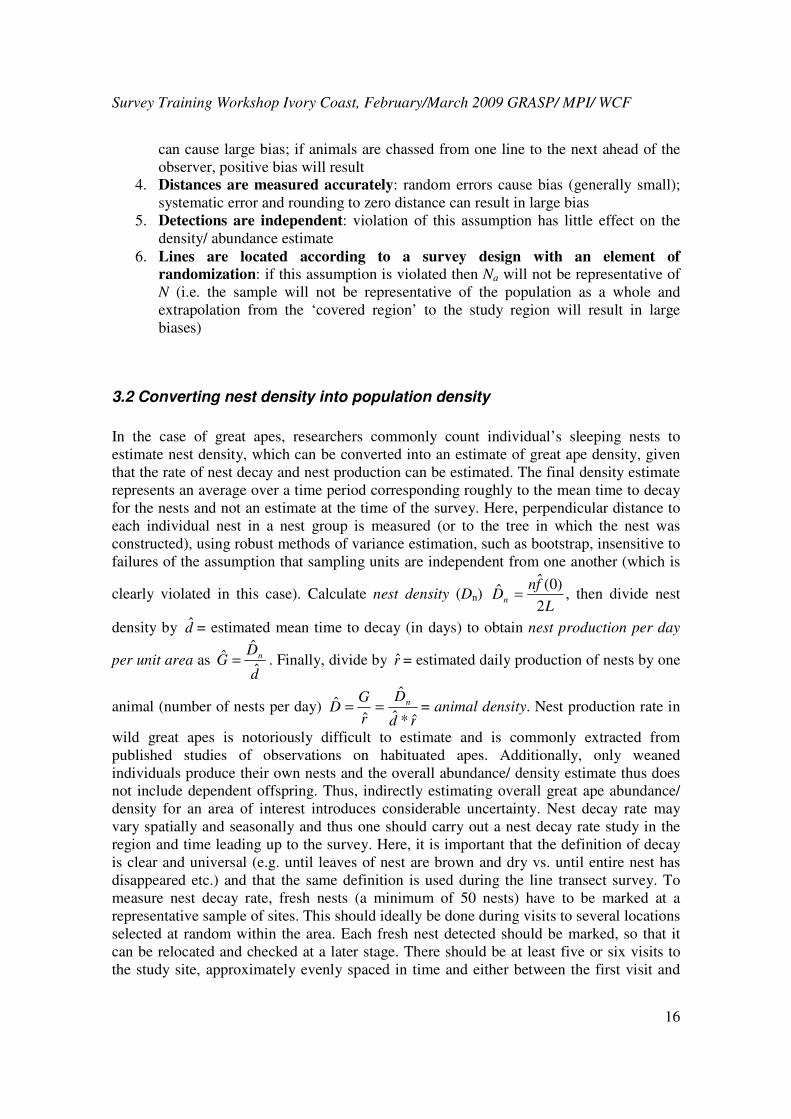
3.2 Converting nest density into population density
In the case of great apes, researchers commonly count individual’s sleeping nests to
estimate nest density, which can be converted into an estimate of great ape density, given
that the rate of nest decay and nest production can be estimated. The final density estimate
represents an average over a time period corresponding roughly to the mean time to decay
for the nests and not an estimate at the time of the survey. Here, perpendicular distance to
each individual nest in a nest group is measured (or to the tree in which the nest was
constructed), using robust methods of variance estimation, such as bootstrap, insensitive to
failures of the assumption that sampling units are independent from one another (which is
clearly violated in this case). Calculate nest density (Dn) L
fnDn
2
)0(ˆˆ = , then divide nest
density by d̂ = estimated mean time to decay (in days) to obtain nest production per day
per unit area as d
DG n
ˆ
ˆˆ = . Finally, divide by r̂ = estimated daily production of nests by one
animal (number of nests per day) rd
D
r
GD n
ˆ*ˆ
ˆ
ˆˆ == = animal density. Nest production rate in
wild great apes is notoriously difficult to estimate and is commonly extracted from
published studies of observations on habituated apes. Additionally, only weaned
individuals produce their own nests and the overall abundance/ density estimate thus does
not include dependent offspring. Thus, indirectly estimating overall great ape abundance/
density for an area of interest introduces considerable uncertainty. Nest decay rate may
vary spatially and seasonally and thus one should carry out a nest decay rate study in the
region and time leading up to the survey. Here, it is important that the definition of decay
is clear and universal (e.g. until leaves of nest are brown and dry vs. until entire nest has
disappeared etc.) and that the same definition is used during the line transect survey. To
measure nest decay rate, fresh nests (a minimum of 50 nests) have to be marked at a
representative sample of sites. This should ideally be done during visits to several locations
selected at random within the area. Each fresh nest detected should be marked, so that it
can be relocated and checked at a later stage. There should be at least five or six visits to
the study site, approximately evenly spaced in time and either between the first visit and

Survey Training Workshop Ivory Coast, February/March 2009 GRASP/ MPI/ WCF
17
the eventual line transect survey, but preferably simultaneous to the survey. A minimum of
50 dung piles over the duration of the decay study should be located.
After marking the nests, only one subsequent visit is required to each nest. The
recorded data will be binary: either the nest has decayed (and is not visible/ can’t be found
anymore – depending on what the definition of decay is) or the nest has not yet decayed
(scoring: 0 or 1, respectively). A logistic regression can then be carried out on these data,
with time elapsed between marking and revisiting the nest as the covariate (Fig. 7).
Mean time to decay can then be estimated by differentiating the distribution function to
give the pdf f(t) say of time to decay, from which mean time to decay is estimated by
numerical integration: dtttfT )(0∫ , where T is some arbitrarily large elapsed time
(corresponding to the maximum plausible time to decay). Variables other than nest age
(e.g. tree species, daily rainfall) may improve estimation of mean time to decay and also be
included in the logistic regression.
3.3 Survey design
When planning a survey it is important to have clear objectives. Once objectives and
anticipated outcome of the survey has been stated clearly, one can decide what levels of
precision and what resources will be required to achieve those objectives. For example, if
the aim was to detect trends in rates of population change over time, we would want to
obtain estimates with high precision. Here, it may be less important to obtain estimates that
are close to true population size (i.e. accurate). To minimize variance between estimates
and thus ensure high levels of precision, such a survey would use the same transects during
each survey event. If, however, the aim of the survey was to obtain an accurate abundance
estimate, then one would vary transect locations to achieve a better coverage of the area of
interest, thereby increasing accuracy of the estimate.
Fig. 7 Logistic regression of percentage of nests surviving decay as a function of time,
based on binary nest decay data (red “X”)
Nest
decay
score
1
Time
0
0

Survey Training Workshop Ivory Coast, February/March 2009 GRASP/ MPI/ WCF
18
Before conducting a survey, it is also important to ensure that observers are well
trained and that a pilot study is conducted to gain some knowledge of the area and to
gather some preliminary information on the distribution and density of the animals to be
surveyed. The following points should be considered when deciding on a sampling design:
• Line transect locations should be chosen at random, or by using a systematic grid of
lines, randomly superimposed on the study area
• Roads and tracks should not be used as transects and the study area should be
stratified if strong differences in habitat or density are apparent
• Lines should be orientated perpendicular to density contours (parallel to density
gradients) or to linear features (Fig. 8)
• The use of a buffer zone can aid in eliminating edge effects (important for
relatively small areas)
• Systematic grid of short lines with adjustment avoids partial lines at the edge
• A circuit design can improve efficiency of time spent in the field (when adopting
such a design a unified and clearly defined survey protocol is very important
• One should aim for at least 60-80 sightings for fitting the detection function
• One should aim for at least 20 line transects for estimating encounter rate (n/L),
where total line length should be determined according to level of precision needed
to achieve specific research/management objectives
Low
High
Density
gradient
Line
transects
Fig. 8 Study area showing a vertical nest (indicated by “X”) density gradient. Line
transects are located parallel to this gradient and systematically cover the entire
region. Adopting such an approach reduces variance in nest encounter rates between
transects, thereby increasing the precision of estimates

Survey Training Workshop Ivory Coast, February/March 2009 GRASP/ MPI/ WCF
19
Recces
Recces or reconnaissance walks are “paths of least resistance”. In areas that are remote,
extremely large, or where dense vegetation hampers passage thereby slowing down the
process of data collection, recces may be walked in combination with line transects (or
during pilot studies). For instance, recces may be walked between subsequent transects, i.e.
while walking to the next transect (Fig. 9). Such a survey design would maximize time
spent collecting data in the field. Recces can be along human trails, up water-courses, etc.
Recces are not restricted to movement in a straight line. Although recces cannot be used to
estimate density (they are not representative of the area as a whole), the data collected
during recce walks may serve as indices of abundance and human activities, and be useful
for mapping the distribution of vegetation types. Data collection during recce walks is very
similar to that on line transects. Information on great ape sightings, dung, nests, tracks,
etc., vegetation types and human signs is recorded as for line transect data. One could
either decide to treat recces as strip transects, where one would record nests within a fixed
width off the center of the recce path, or as line transects and measure perpendicular
distances to each nest detected. One could then compare the data and evaluate the
relationship between recce data and great ape densities estimated from line transect data.
When walking a recce, make sure you have activated the track log option on your
GPS. The location of the start and the end point of the recce should be marked, as well as
any prominent points likely to feature on maps (e.g. villages, poacher’s camps etc., river
confluences) and all nest sites. You should note the time you start moving in the morning,
the time you stop at the end of the day and distances and times of any rest periods. Also
keep a careful note of general circumstances (e.g. short of food, team tired etc.) and note
time at each 1 km covered. You should also collect data on vegetation type, slope, altitude
and prominent physical features and note whether you are traveling on a human trail, on a
major elephant path, on minor game trails or cross-country on a compass bearing as well as
the location, size (major, medium, minor), state (is it swept clear by passage of animals –
active; are leaves accumulating – recent use; or is it abandoned) and the direction of
elephant trails.
Fig. 9 Study design including line transect circuits (solid lines) and recces
(stippled lines) walked between each line transect circuit. The study area is
indicated in green.
Recces
Line transect circuits

Survey Training Workshop Ivory Coast, February/March 2009 GRASP/ MPI/ WCF
20
3.4 Introduction to analysis in Distance 5.0
Les projets dans Distance sont typiquement enregister comme des fichiers zip. Pour les
dézziper et ouvrir un projet à partir fichier zippé, aller simplement à “Fichier/Ouvrir et
sélectionner un projet de l’archive des fichiers zippés. Les données d’étude dans Distance
sont separées en differents couches de données. Celles-ci sont la couche globale (e.g.
l’habitat en entier/ Zone d’étude), le strate layer (e.g. different habitats), the sample layer
(the line transect) and the observation layer (detections).
Click on “Start”. A list will be displayed. Click on “Programs”, then “Distance”. Now
click on “Distance 5”. Refer to the exercise 2 folder. These data have been set up as a
distance project, which have been archived and compressed as a .zip file on your CD under
“Workshop documents & exercises\Exercises”. Select “File” followed by “Open project”.
Under “Files of type” choose “Zip archive files (*.zip)”. Next to “Look in”, browse for the
file “Exercise A” on your CD/ DVD drive “E:” (or wherever you have saved this
document). Double-click on “Ducknest exercise.zip”. Click “OK” to unpack the project
into the current directory and open it. Next time you open the project, you can open the file
“Ducknest exercise.dst” directly.
Global Stratum Sample
Observation
Field name
Field type
(integer,
decimal, text,
ID, label)
Units
Data source
(internal,
geographic)
Survey Training Workshop Ivory Coast, February/March 2009 GRASP/ MPI/ WCF
21
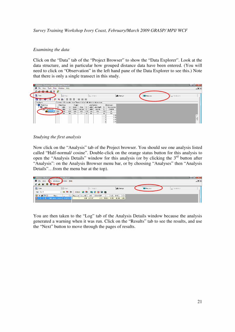
Examining the data
Click on the “Data” tab of the “Project Browser” to show the “Data Explorer”. Look at the
data structure, and in particular how grouped distance data have been entered. (You will
need to click on “Observation” in the left hand pane of the Data Explorer to see this.) Note
that there is only a single transect in this study.
Studying the first analysis
Now click on the “Analysis” tab of the Project browser. You should see one analysis listed
called “Half-normal/ cosine”. Double-click on the orange status button for this analysis to
open the “Analysis Details” window for this analysis (or by clicking the 3rd
button after
“Analysis”: on the Analysis Browser menu bar, or by choosing “Analyses” then “Analysis
Details”…from the menu bar at the top).
You are then taken to the “Log” tab of the Analysis Details window because the analysis
generated a warning when it was run. Click on the “Results” tab to see the results, and use
the “Next” button to move through the pages of results.

Survey Training Workshop Ivory Coast, February/March 2009 GRASP/ MPI/ WCF
22
Creating a new analysis
Return to the Analysis browser and click on the first button after “Analysis” on the
Analysis browser menu bar (“New Analysis”). Double-click on the status button to go to
the Analysis Details window for this new analysis.
Because the analysis is not run yet, you are taken back to the “Inputs” tab. You will not
need to edit the Survey or Data Filter for this example, but click on “New” in the “Model
Definition” section.

Survey Training Workshop Ivory Coast, February/March 2009 GRASP/ MPI/ WCF
23
Explore the options and try changing one or more, for example specifying a different
model for the detection function. When you have defined your new model, give it a
suitable name (one that reflects the options you have set) and select “OK”.
Now click the “Run” button. When the analysis finishes, it will automatically take you to
the “Log” tab if there were problems or the “Results” tab if the analysis ran without errors
or warnings. From the results tab, you can investigate the results of your analysis.
Further investigations
Try creating several different analyses, each with different model definitions and compare
their performances. Note: when you create a new analysis (or model definition or data
filter), Distance copies the settings from whichever analysis (or model definition or data

Survey Training Workshop Ivory Coast, February/March 2009 GRASP/ MPI/ WCF
24
filter) was highlighted at the time (the name is also copied). The default settings are not
restored automatically. It is easiest to compare results from different analyses using the
Analysis browser. You can change the default columns in the browser using the “Column
manager” (furthest button on the right of the Analysis browser menu bar).
You can also change the order of the analyses, rename them or delete them using the
Analysis Components window by clicking the 6th
button from the right on the main menu
bar (“View Analysis Components”). In the Analysis Components window, the first button
lists the Data Filters and the second button lists the Model Definitions.

Survey Training Workshop Ivory Coast, February/March 2009 GRASP/ MPI/ WCF
25
You can also enter data manually by using the Data Entry Wizard. Open a new project
(click on “File” and “New project”…), name it and click on “Create”. Step through the
New Project Wizard (you should not need to change any of the defaults, but study each
page) and click on “Finish”. This takes you to the Data Entry Wizard. Click “Next” until
you get to the “line transect” page. Enter say the first 6 line labels (e.g. “line 1”, “line 2”
…) and lengths (5, 2 …). You need to click on the “append new record after current”
button on the menu bar before entering the information for each line.
When you have finished, click next and enter the distances corresponding to each
observation in a similar fashion. Once you have entered the distance data, you can go to
the analysis browser and carry out your analysis.
Please refer to the users guide pdf version in the Distance 5.0 “help” menu for more
detailed information on the program.
4. Introduction to temporal inferences
There are different ways to measure population changes over time: 1) measure change
between two points in time, 2) measure population trends/ tendency (more than 2 points),
3) focus on most recent observation to detect early warning of population change 4) fit
stochastic population dynamics models to the data (conduct population modeling). One
would use different statistical methods for the different types of temporal inferences.
Let’s focus on measuring population trends. Why is it important to monitor
population changes over time? Population trends summarize a population’s response to
extrinsic (e.g. anthropogenic factors) and intrinsic forces (e.g. density, disease) and
frequently form the basis for management decisions. Populations may decrease, increase or
remain stable over time. Simple linear regression on log-transformed data is commonly
used to describe population trends. This method is useful for initial analysis or short time

Survey Training Workshop Ivory Coast, February/March 2009 GRASP/ MPI/ WCF
26
series. It is relatively easy to perform and summarizes a trend as one number. However, the
method is based on several assumptions that may be difficult to meet (assumes errors are
independent, trend is constant over time and population process is random), so more
sophisticated methods should be used for longer time series of estimates.
While the α-level (see section 2.10) controls for Type 1 errors (i.e. falsely rejecting
a null-hypothesis or detecting a trend when the population is actually stable), Type 2 errors
(i.e. falsely accepting a wrong null-hypothesis or not detecting a trend when there is a
trend) a major problem in trend analyses. The probability of detecting a trend when there is
a trend is called statistical power. If we have low power to detect trends in time series of
population estimates, small populations could go extinct without us ever noticing (because
we would think the population is stable). Power is influenced by: 1) the precision of
estimates; 2) the rate of population change to be detected; 3) the number of estimates in
time series; 4) the significance level α. Thus, it is important to consider statistical power
when designing a survey.
For instance, one could use the program TRENDS.exe
(http://swfsc.noaa.gov/textblock.aspx?Division=PRD&ParentMenuId=228&id=4740) to
estimate power for different levels of precision (Fig. 10a). Here, the user specifies
variables 2-3 and varies the level of precision (measured by CV) to estimate statistical
power to detect trends. If some information on nest encounter rates is available, one can
estimate how CV is influenced by survey effort (Lt) (that is total transect length) by using
the equation:
0
0
n
L
L
qCV
t
= and varying Lt, where q is a constant (we assume it to be
3), and L0 is total transect length of the pilot study and n0 is the total number of detections
(e.g. nests) during the pilot study (Fig. 10b). One can then determine minimum transect
length to achieve the desired CV and ensure sufficient power to detect trends.
West Africa (nests)
0
0.05
0.1
0.15
0.2
0.25
0.3
0.35
0 50 100 150 200 250 300 350 400
Survey effort (km)
CV
0
0.1
0.2
0.3
0.4
0.5
0.6
0.7
0.8
0.9
1
0 0.1 0.2 0.3 0.4 0.5 0.6 0.7 0.8 0.9 1
CV
PO
WE
R
50% change over 5 years
50% change over 10 years
50% change over 15 years
a b
Fig. 10 a) Power to detect trends after 5, 10 and 15 years at varying levels of
precision. Sufficient power is routinely set at 0.8 (80% chance of detecting a trend
when in fact there is a population change). In order to yield sufficient power to
detect a 50% population change (e.g. decline) after 5 years, we require a CV of no
more than 0.1 (10%). This means that we would have to b) survey at least 100 km
of transects. In this case, by the time we detected this 50% population change, the
population may already be extinct.

Survey Training Workshop Ivory Coast, February/March 2009 GRASP/ MPI/ WCF
27
5. Introduction to spatial analyses using ArcView-ArcMap
Geographic Information Systems (GIS) help you to manage, analyze, and present spatial
information. GIS allows you to combine several layers that include data on the physical
environment with biological information (e.g. nest detections) collected in the field.
Researchers can benefit from the use of a GIS to investigate data visually and develop
spatially accurate graphical data displays. By presenting data in form of a map, spatial
patterns may be revealed that would have been difficult to illustrate in a table of rows and
columns. Spatial application of empirical data could possibly aid researchers in decision-
making that could lead to a better understanding of biological systems.
Adding a shapefile (refer to the “ArcGIS” folder for importing GIS data)
Shapefiles contain geodata and were specifically designed for ArcGIS. Each shapefile
contains a minimum of three files: 1) .shp, 2) .shx and 3).dbf files. Shapefiles can include
either points, lines (polylines) or surfaces (polygons). Open ArcMap on your computer
(either via the “Start” menue or through a shortcut link on your desktop. To add a polygon
of your study area (let’s assume this is Taï National Park), click on the “add data” icon on
the toolbar and choose the destination to the file that contains the shapefile with the
polygon (or polyline) of your study area.

Survey Training Workshop Ivory Coast, February/March 2009 GRASP/ MPI/ WCF
28
You will see that as soon as you add the polygon, it will show as a layer in the layers
window on the left hand side. Note the tick in the box next to the layer’s name – if you
‘untick’ the layer you inactivate it and it will no longer show in the data view window.
“Add data”
icon

Survey Training Workshop Ivory Coast, February/March 2009 GRASP/ MPI/ WCF
29
You can change the layer properties by ‘right-clicking’ on the
layer name and choosing ‘Properties’ from the menu. Here, you
can change the appearance of the information by changing
properties in the “Symbology” sub-menu.
Uploading GPS points

Survey Training Workshop Ivory Coast, February/March 2009 GRASP/ MPI/ WCF
30
To add GPS data (e.g. transects and the total number of nests per transect), you first have
to store the information (Longitude and Latitude and total number of nests per transect) in
an Excel sheet in the format .dbf or . txt.
Then click on “Tools” and choose “add XY data” from the menu. A window appears that
allows you to choose the Excel table from your file and to specify the fields for the X
(Longitude) and Y (Latitude) coordinates. Here, you can also specify the Coordinate
System of the Input file (e.g. UTM or degrees). Click “OK” to add your GPS points to the
map.
You now have to export the sheet that was added to the layer view to store it as a file on
your computer. Right-click on the sheet’s name and choose “Data” and then “Export data”.

Survey Training Workshop Ivory Coast, February/March 2009 GRASP/ MPI/ WCF
31
Give a name to this file (e.g. Taï data points), specify the file destination for where you
would like to store this information and click “OK”.
Interpolation
This new layer that we called “Tai data points” includes more
information than just the coordinates of the line transects that you
walked. It also includes nest count data (i.e. the number of nests per
transect). You can look at the data included in each layer by right-
clicking on the layer’s name and choosing “Open attribute table”
from the menu. One way of displaying nest density data is by
creating an interpolation surface. Interpolation is the method used to
estimate an unknown value at a certain point using the sampling
values, regardless of this point being \inside" or \outside" the
sampling points (the last case is often referred to as extrapolation).
This means that, based on the nest count data collected in Tai
National Park, we can predict nest densities for areas for which we
have not collected any information (area not covered by line
transects). Click on “Spatial analyst tools”, “Interpolation” and then
“Spline with barriers”. There are several different interpolation
methods you can use. To choose the correct method and to read
about what each method does, refer to the document “Interpolating
surfaces in ArcGIS”, which is stored as a pdf file on the CD you
received for this course. A window will appear that allows you to
specify the “Input point features” (this is the shapefile “Tai data points” that includes the
nest count data), the name of the column in the file that includes the data, which is referred
to as the “Z value field” (this is the column with the name “Total” includes total number of
Survey Training Workshop Ivory Coast, February/March 2009 GRASP/ MPI/ WCF
32
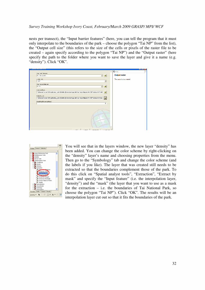
nests per transect), the “Input barrier features” (here, you can tell the program that it must
only interpolate to the boundaries of the park – choose the polygon “Tai NP” from the list),
the “Output cell size” (this refers to the size of the cells or pixels of the raster file to be
created – again specify according to the polygon “Tai NP”) and the “Output raster” (here
specify the path to the folder where you want to save the layer and give it a name (e.g.
“density”). Click “OK”.
You will see that in the layers window, the new layer “density” has
been added. You can change the color scheme by right-clicking on
the “density” layer’s name and choosing properties from the menu.
Then go to the “Symbology” tab and change the color scheme (and
the labels if you like). The layer that was created still needs to be
extracted so that the boundaries complement those of the park. To
do this click on “Spatial analyst tools”, “Extraction”, “Extract by
mask” and specify the “Input feature” (i.e. the interpolation layer,
“density”) and the “mask” (the layer that you want to use as a mask
for the extraction – i.e. the boundaries of Tai National Park, so
choose the polygon “Tai NP”). Click “OK”. The results will be an
interpolation layer cut out so that it fits the boundaries of the park.

Survey Training Workshop Ivory Coast, February/March 2009 GRASP/ MPI/ WCF
33
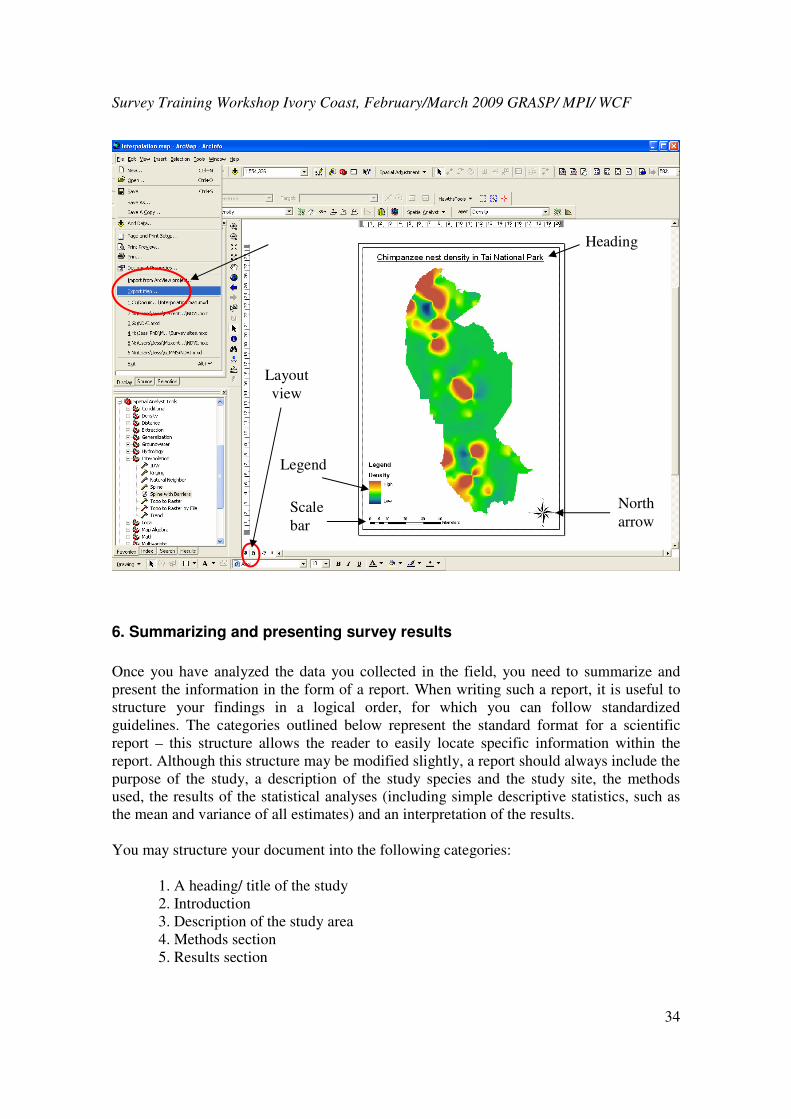
Designing the final map
Finally, you would want to display your data in form of a proper map with a legend, a
scale bar, a North arrow, and a heading. After you have finalized your map, you can print it
out and/or store it as a .jpg image that you can save and store on your computer. The .jpg
image includes a static map, that is, once you have saved it as a .jpg you can’t change the
image again. However, you can change it in ArcMap/View and then export it again and
overwrite the previous image or save it as an additional image. To design your map of e.g.
chimpanzee nest density in Tai National Park, first change from “Data view” (which is the
active view you are in at the moment) to “Layout view”. To insert a scale bar, the legend
and a North arrow, click on “Insert” and choose “Scale bar”, “Legend” and “North arrow”,
respectively. Once inserted, you can change the properties of each icon (e.g. set the unit for
the scale bar to kilometers) by double-clicking on the icon. You can add a heading to your
map by clicking on “Insert” and choosing “Text” from the menu. When you are finished
with editing your map, click on “File” and choose “Export file” from the menu to export
your map as a .jpg image and save it on your computer. In the window that appears specify
the file format for the output file (i.e. .jpg) and click “OK”.
Survey Training Workshop Ivory Coast, February/March 2009 GRASP/ MPI/ WCF
34
6. Summarizing and presenting survey results
Once you have analyzed the data you collected in the field, you need to summarize and
present the information in the form of a report. When writing such a report, it is useful to
structure your findings in a logical order, for which you can follow standardized
guidelines. The categories outlined below represent the standard format for a scientific
report – this structure allows the reader to easily locate specific information within the
report. Although this structure may be modified slightly, a report should always include the
purpose of the study, a description of the study species and the study site, the methods
used, the results of the statistical analyses (including simple descriptive statistics, such as
the mean and variance of all estimates) and an interpretation of the results.
You may structure your document into the following categories:
1. A heading/ title of the study
2. Introduction
3. Description of the study area
4. Methods section
5. Results section
North
arrow Scale
bar
Legend
Heading
Layout
view

Survey Training Workshop Ivory Coast, February/March 2009 GRASP/ MPI/ WCF
35
6. Interpretation and discussion section
7. Recommendations
8. Conclusions (or summary)
9. Figures and tables
In the introduction, you need to introduce the study topic to the reader. Here, you need to
state the purpose/ objective of your study (e.g. “to estimate chimpanzee density across Tai
National Park” or “to estimate rates of change in the chimpanzee population in Tai
National Park”). Here, it may be useful to ask yourself the following three questions: (1)
What is the problem? (2) Why is it a problem? (3) What did I do about the problem?
You also need to provide background information relevant to the purpose of the
study. For example, you may inform the reader about results of previous studies conducted
in the same area and/ or on the same study animal or survey method. You may also want to
include information that led you to conduct the study in the first place – for example, you
may refer to a study that reported an increase in poaching in the study area that led you to
investigate the potential negative effect thereof on the ape population living in the area.
You should then provide a brief description (and a map) of the study area. Here, the
following types of information can be included:
• Geographic coordinates of the study area
• Location of the study area relative to regional habitat types and topographic
features (for example, “The study lies less than 40 km away from the ocean to the
west and borders a mountain range (provide the name of the mountain range) to the
east”)
• Local topography (hilly, flat etc.), distinct features (rivers, mountains etc.), range of
elevations within the study area, a summary of local geography and soil types
• Habitat types and animals found within the study area, possibly including a list of
common plant and animal species
• Average annual rainfall and average maximum and minimum temperatures in or
near the study area
• Background about local ethnic groups and their histories
In the methods section you need to give a detailed description of the methods that you used
to obtain your results (i.e. how exactly did you collect your data in the field?). The
description should be detailed enough to allow the reader to repeat the study. This is
important, because it allows the reader to assess how appropriate the methods were, to use
the same methods for a similar purpose and to compare your results with those of other
studies that used similar methods. If you conducted a line transect survey, the following
information should be included:
• Dates and times of when the data were collected
• Location of transects (if possible provide geographic coordinates), specifically
relate their locations to those of any rivers, mountains, villages, trails, logged areas,
secondary forest etc. (here, it is best to use a map)
• Length of transects
• Number of transects
Survey Training Workshop Ivory Coast, February/March 2009 GRASP/ MPI/ WCF
36
In the results section, you need to summarize the data together with a description of any
patterns or trends detected in the results. To do this, you should make use of tables, figures
and/or maps, where appropriate and follow standardized methods for reporting statistical
results. In the case of line transect surveys you may include the following information:
• Total number of animals/ nests detected
• Mean (here, also report the sample size and standard deviation) number of animals
nests detected per kilometer walked (i.e. nest encounter rate)
• Range of the number of animals/ nests detected per transect walked
• Animal/ nest density (per square kilometer)
• Density for each habitat type
In the discussion section of your report you need to objectively interpret and critically
evaluate your results. Here, you should compare your results to those obtained by other
relevant studies (e.g. those conducted in other areas, or at other times, or with different
species). Write about what interesting things you know now that you have conducted the
study that you did not know before, or what implications the results of your study have for
the management and conservation of the species/ area that you studied. All conclusions
should be based on the results of your study and all arguments for AND those that
contradict your conclusions should be stated. Highlight what you have found to be of
greatest significance. Most importantly, the discussion should answer (or say why it does
not answer) the question(s) posed in the introduction. If you stated hypotheses in your
introduction, you should reject (or accept) these and explain why your results do (or do
not) support your hypotheses. The end of the report should always state if any advance has
been made by the study on the situation or state of knowledge before the study began (i.e.
Why was this study important and has this study achieved its anticipated outcomes?).
The introduction, methods, results and discussion sections should all follow the same
structure and logical sequence of arguments.
In the recommendations section, give recommendations (based on your experience during
the study and your results) on how to improve future studies. Here, you may also make
recommendations for management and conservation of the species/ area you studied. In
this section you should illustrate the practical implications of your work and suggest
courses of action which need to be followed or new lines of research, which are considered
to be a priority (e.g. perhaps you found that nest decay rate for your study area was much
higher when compared to studies of nest decay elsewhere, you may want to suggest that
future surveys measure site-specific nest decay rates in order to establish a firm
relationship which can be applied to density estimations).
Last, briefly summarize your results and conclusions in the summary section of your
report. Add your figures and tables to the end of the report. It is important that you number
and label each table (heading) and figure (legend below the figure) and that you refer to all
figures and tables in the text appropriately.

Survey Training Workshop Ivory Coast, February/March 2009 GRASP/ MPI/ WCF
37
7. Collection of organic samples for DNA analysis
The collection of organic samples as a source of DNA such as feces, hair, sperm plugs
and/or food remains represents a non-invasive method for obtaining data used for genetic
analysis of paternity, relatedness, and dispersal. Additionally, information on population
size and genetic structure, sex ratio, group structure and composition, home range size,
habitat use, and diet may be extracted from these samples. Hormone and other
physiological parameters may contain information on e.g. reproductive status, health and
stress levels of great apes. These samples should be collected during line transect surveys
where additional people look specifically for ape dung. Here people may leave the transect
line and look for the dung in surrounding areas if they hear/see apes nearby. Methods for
collecting and storing samples are as follows:
Materials needed
• 50 mL tubes containing silica gel beads
• Ethanol (pharmacy grade, 97%), 90% should also work
• Empty 50 mL tubes
Preparation
• Pour approximately 30 ml of ethanol into empty tubes for sample collection.
Collection
• Collect each fresh feces sample (approx 5 g) into a tube containing ~ 30 ml
ethanol
• Label, but remember this tube will be discarded (location, date, transect, age of the
sample, unique ID number that links to more detailed information for this organic
sample (species), (age of the animal), (sex of the animal)
Processing (next day)
The bolus of the fecal sample collected into ethanol should be transferred into fresh silica
tubes for further drying. This can be done by carefully pouring off the ethanol with the
tube loosely capped and using Kimwipes to transport solid material to the new tube. This
tube should be labelled preferably in a manner that indicates the ethanol step was used (for
example, 159E). Store sample at room temperature.

Survey Training Workshop Ivory Coast, February/March 2009 GRASP/ MPI/ WCF
38
8. A Pan-African ape trend estimation program
Summary
Information on rates of population change and factors influencing great ape populations in
different regions is key to informing and evaluating management decisions to ensure their
protection. However, despite considerable effort and resources devoted to the systematic
monitoring of their populations over nearly 30 years, to date few data are available that
allow for the precise estimation of population trends by country or region. In addition,
there is a need to centralise existing survey information valuable for trend analyses and
make it easily accessible to the conservation and scientific community.
As the establishment of site-specific, intense monitoring programs is expensive and
a relatively slow process, we propose an alternative approach to provide regional trend
estimates of ape populations in a relatively short amount of time. This can be done by
revisiting previous sampling locations and combining them with ongoing field programs.
Integrated in the long-term objective for setting up a sensitive and efficient Pan African
great ape trend estimation program, this project aims to achieve the following objectives:
1. To identify previous sampling sites across Africa for which chimpanzee survey
data are available using the IUCN/SSC/PSG/SGA A.P.E.S. database
(http://apes.eva.mpg.de).
2. To identify “negative hotspots” of potential great ape population decline across
their range (high rates of deforestation and human population growth).
3. To develop a robust sampling design for all great ape range countries in Africa that
is sensitive enough to detect rates of population change of at least 20% and that
combines previous sampling locations, ongoing field programs and “negative
hotspots”.
4. To sample pre-determined priority locations and deliver immediate trend estimates,
as well as determine the relative importance of underlying factors causing the
observed population trend. During the first phase of this project we will concentrate
on the largest West African chimpanzee populations (Sierra Leone, Guinea, Côte
d’Ivoire and Liberia) thereafter expanding to Central and East African range
countries.
5. To present results in a time efficient manner online in the IUCN/SSC/PSG/SGA
A.P.E.S. database.
The project that will be jointly executed by the Wild Chimpanzee Foundation (WCF) and
the Department of Primatology of the Max Planck Institute of Evolutionary Anthropology
in Leipzig, will use the methodology of standard line transect nest count sampling.
Temporal trend estimates will be derived by comparing nest (group) encounter rates and if
data allow also nest (group) densities. Spatial trends and their underlying causes (threats
and protective factors) will be evaluated using a model based approach. The project will be
integrated into ongoing monitoring activities in the respective countries. Contacts to the
organizations involved in monitoring work already exist or will be established in the period
leading up to this project. It will support regional capacity building through practical and
analytical training of national field staff and national wildlife biologists, and will provide

Survey Training Workshop Ivory Coast, February/March 2009 GRASP/ MPI/ WCF
39
essential information for strategic conservation planning in the region. Regional
chimpanzee population trend estimates and information on underlying causes will be
stored in the IUCN/SSC/PSG/SGA A.P.E.S. database and made available on the
IUCN/SSC/PSG/SGA A.P.E.S. website (http://apes.eva.mpg.de).
9. The IUCN/SSC/PSG/SGA A.P.E.S. database
Since 25 years numerous ape surveys have been conducted in order to asses the
occurrence, spatial distribution and abundance of bonobo, chimpanzee, gorilla and orang-
utan populations. But the use of different monitoring techniques and the rapid
disappearance of suitable ape habitat all over the world make it very difficult to get a
coherent picture of the plight of the apes. Existing ape survey data hold valuable
information about the apes’ status in different regions of the world. A hurdle in using this
information is the dispersal of data across many countries, organizations & institutions and
the lack of a uniform (digital) data format, thus making it hard to access and compare.
Considering the high costs of ape surveys and the urgent need for more detailed
information about (local) trends in ape populations make it desirable to dispose of an
efficient tool allowing the coordination of survey effort and storage of existing data for
spatial/temporal trend analysis of ape populations.
The aim of the IUCN/SSC/PSG/SGA A.P.E.S. database is to create a web-based
platform storing all existing (un-) processed ape survey data in a standardized format to
facilitate spatial/ temporal trend analysis of ape populations, from a local to a large scale.
In addition, information on each great ape conservation site, population status and surveys
can be accessed via the A.P.E.S. “Wiki”. Here, the user can easily navigate through
regions, countries and sites. The goal of the A.P.E.S “Wiki” is to provide extensive
qualitative information about the status of each ape population to complement the
quantitative information contained in the survey datasets archived in A.P.E.S.
9.1 Editing information on the IUCN/SSC/PSG/SGA A.P.E.S. website
The A.P.E.S. Wiki is an interactive site and allows the user to contribute and edit
information on the website. People are in possession such data and would like to contribute
these, can log-in with the following log-in details:
Username: User
Password: apeswiki12

Survey Training Workshop Ivory Coast, February/March 2009 GRASP/ MPI/ WCF
40
Once logged-in, the user can navigate to the site of interest and edit and/or add information
under the different headings: “Site”, “Ape status”, “Threats”, “Conservation activities”,
“Surveys”. The user may provide a reference for the added information in the “Reference”
section or list the information under “Name X, Year XXXX, personal communication”.
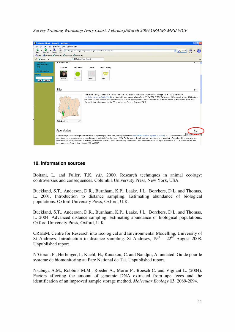
Survey Training Workshop Ivory Coast, February/March 2009 GRASP/ MPI/ WCF
41
10. Information sources
Boitani, L. and Fuller, T.K. eds. 2000. Research techniques in animal ecology:
controversies and consequences. Columbia Universuty Press, New York, USA.
Buckland, S.T., Anderson, D.R., Burnham, K.P., Laake, J.L., Borchers, D.L. and Thomas,
L. 2001. Introduction to distance sampling. Estimating abundance of biological
populations. Oxford University Press, Oxford, U.K.
Buckland, S.T., Anderson, D.R., Burnham, K.P., Laake, J.L., Borchers, D.L. and Thomas,
L. 2004. Advanced distance sampling. Estimating abundance of biological populations.
Oxford University Press, Oxford, U.K.
CREEM, Centre for Research into Ecological and Environmental Modelling, University of
St Andrews. Introduction to distance sampling. St Andrews, 19th
– 22nd
August 2008.
Unpublished report.
N’Goran, P., Herbinger, I., Kuehl, H., Kouakou, C. and Nandjui, A. undated. Guide pour le
systeme de biomonitoring au Parc National de Tai. Unpublished report.
Nsubuga A.M., Robbins M.M., Roeder A., Morin P., Boesch C. and Vigilant L. (2004).
Factors affecting the amount of genomic DNA extracted from ape feces and the
identification of an improved sample storage method. Molecular Ecology 13: 2089-2094.
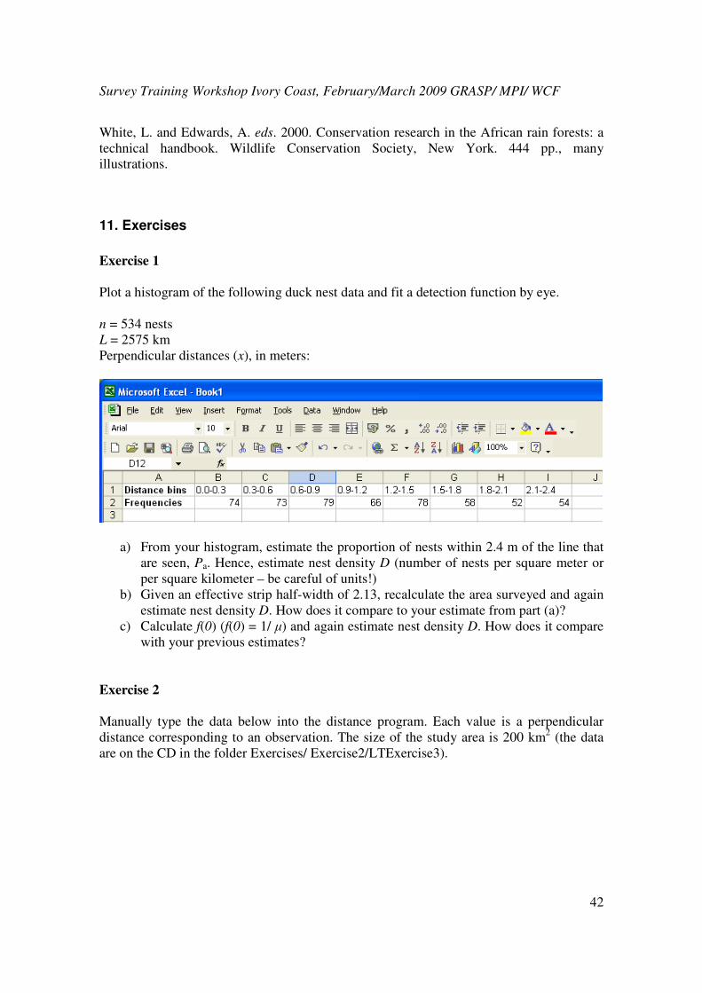
Survey Training Workshop Ivory Coast, February/March 2009 GRASP/ MPI/ WCF
42
White, L. and Edwards, A. eds. 2000. Conservation research in the African rain forests: a
technical handbook. Wildlife Conservation Society, New York. 444 pp., many
illustrations.
11. Exercises
Exercise 1
Plot a histogram of the following duck nest data and fit a detection function by eye.
n = 534 nests
L = 2575 km
Perpendicular distances (x), in meters:
a) From your histogram, estimate the proportion of nests within 2.4 m of the line that
are seen, Pa. Hence, estimate nest density D (number of nests per square meter or
per square kilometer – be careful of units!)
b) Given an effective strip half-width of 2.13, recalculate the area surveyed and again
estimate nest density D. How does it compare to your estimate from part (a)?
c) Calculate f(0) (f(0) = 1/ µ) and again estimate nest density D. How does it compare
with your previous estimates?
Exercise 2
Manually type the data below into the distance program. Each value is a perpendicular
distance corresponding to an observation. The size of the study area is 200 km2 (the data
are on the CD in the folder Exercises/ Exercise2/LTExercise3).
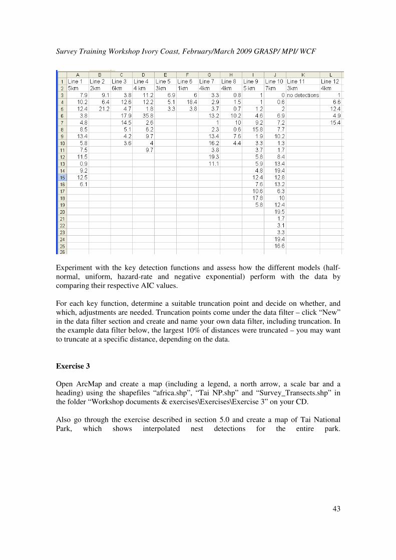
Survey Training Workshop Ivory Coast, February/March 2009 GRASP/ MPI/ WCF
43
Experiment with the key detection functions and assess how the different models (half-
normal, uniform, hazard-rate and negative exponential) perform with the data by
comparing their respective AIC values.
For each key function, determine a suitable truncation point and decide on whether, and
which, adjustments are needed. Truncation points come under the data filter – click “New”
in the data filter section and create and name your own data filter, including truncation. In
the example data filter below, the largest 10% of distances were truncated – you may want
to truncate at a specific distance, depending on the data.
Exercise 3 Open ArcMap and create a map (including a legend, a north arrow, a scale bar and a
heading) using the shapefiles “africa.shp”, “Tai NP.shp” and “Survey_Transects.shp” in
the folder “Workshop documents & exercises\Exercises\Exercise 3” on your CD.
Also go through the exercise described in section 5.0 and create a map of Tai National
Park, which shows interpolated nest detections for the entire park.

Survey Training Workshop Ivory Coast, February/March 2009 GRASP/ MPI/ WCF
44
2. Appendices
Appendix 1: Example of a survey data sheet
Fiche de collecte de données pour le biomonitoring dans le Parc National de Taï
Date :……………………... Secteur :………...……………....... Transect de base :………..……………. Temps :
……………………………..
Enquêteur :……………………………..…………………..……… Heure départ :……………..................... Heure
arrivée : ………..….…………
Caractéristiques générales de l’observation Position géographique
Tronçon
Transect Heure Type ou code
de l’observation
Vu /
Entendu
Taille gpe-Singes
Dégrad./hauteur
crotte-Eléph
Dégrad. nid-Chimp.
Distance
parcourue
(m)
Distance
perpend.
(m)
Numéro
position
Longitude
(UTM)
Latitude
(UTM)
Remarques et
Commentaires
précisions sur
l'observation

Survey Training Workshop Ivory Coast, February/March 2009 GRASP/ MPI/ WCF
45

Survey Training Workshop Ivory Coast, February/March 2009 GRASP/ MPI/ WCF
46
Appendix 2: Photos of different nest decay stages
Fresh nests (class 1): all leaves in the nest are green and generally feces or urine odors
are underneath the nest
Recent nests (class 2): drying leaves of different colors, green may dominate, but no
dung and no urine odor underneath the nest

Survey Training Workshop Ivory Coast, February/March 2009 GRASP/ MPI/ WCF
47
Old nests (class 3): structure still roughly intact with the majority of leaves brown
Very old nests (class 4): nest with holes showing few or no leaves, but still identifiable by
bent twigs

Survey Training Workshop Ivory Coast, February/March 2009 GRASP/ MPI/ WCF
48
Appendix 3: Map of Taï National Park and surrounds